Competitive Screening under Heterogeneous

Information∗

Daniel Garrett† Renato Gomes‡ Lucas Maestri§

December 12, 2014

Abstract

We study competition in price-quality menus when consumers privately know their valuation

for quality (type), and are heterogeneously informed about the offers available in the market.

While firms are ex-ante identical, the menus offered in equilibrium are ordered so that more

generous menus leave more surplus uniformly over types. More generous menus provide quality

more efficiently and generate a greater fraction of profits from sales of low-quality goods. By

varying the level of informational frictions, we span the entire spectrum of competitive intensity,

from perfect competition to monopoly. More competition may raise prices for low-quality goods;

yet, consumers are better off, as their qualities also increase.

JEL Classification: D82

Keywords: competition, screening, heterogeneous information, price discrimination, adverse

selection

∗We are grateful to Jean Tirole for extensive comments at the early stages of this project. We also thank Yeon-

Koo Che, Andrew Clausen, Jacques Cremer, Wouter Dessein, Jan Eeckhout, Renaud Foucart, Ed Hopkins, Bruno

Jullien, Tatiana Kornienko, Volker Nocke, Wojciech Olszewski, Michael Peters, Patrick Rey, Andrew Rhodes, Mike

Riordan, Maher Said, Ron Siegel, Bruno Strulovici, Andre Veiga, and Yaron Yehezkel for very helpful conversations.

For useful feedback, we thank seminar participants at Bilkent, Columbia, FGV-EPGE, the LMU of Munich, Mel-

bourne, Monash, UNSW, Queensland, Ecole Polytechnique, Northwestern, Oxford, Bonn, Edinburgh, Stonybrook, the

Toulouse-Northwestern IO conference, the UBC-UHK Theory conference (Hong Kong), the CEPR Applied IO confer-

ence (Athens), INSPER, the EARIE conference (Milan), Mannheim, PSE and Pompeu Fabra. The usual disclaimer

applies.†Toulouse School of Economics, daniel.garrett@tse-fr.eu.‡Toulouse School of Economics, renato.gomes@tse-fr.eu.§Getulio Vargas Foundation (EPGE), maestri.lucas@gmail.com.

1 Introduction

Price discrimination through menus of products at different prices is a widespread practice across

many industries. Examples include flight seats with different classes of service, electronic printers

with various processing speeds, and automobiles in standard or deluxe versions.

The benchmark setting where the seller is a monopolist was first studied by Mussa and Rosen

(1978). This paper considers consumers who differ in their appreciation of quality and shows that

the monopolist’s profit-maximizing policy involves downward distortion of quality for all consumers,

except for those who value it the most. Thus purchasers of printers with the highest value for speed

enjoy the efficient speed; all others’ printers are inefficiently slow. The optimal distortions resolve a

trade-off between extracting rents from consumers with high willingness to pay, and providing more

efficient qualities to the others.

Much of the price discrimination we observe in practice occurs, however, not in the textbook

monopoly setting, but in the presence of competition. A range of models have therefore been de-

veloped to study price discrimination in settings where market power is limited by competition;

see, among others, Champsaur and Rochet (1989), Rochet and Stole (1997, 2002) and Armstrong

and Vickers (2001) (the next subsection gives a detailed account of this literature).1 An assump-

tion maintained throughout this body of work, as well as in much of the large empirical literature

on competition with differentiated products following Berry, Levinsohn and Pakes (1995), is that

consumers enjoy perfect (and therefore homogeneous) information about the offers available in the

market.

The aim of our paper, by contrast, is to study competitive price discrimination in settings where

consumers are heterogeneously informed about the offers available in the market. That is, due to

information frictions, consumers differ on which (and how many) firms they know. Aware of the

information heterogeneity among consumers, competing firms offer price/quality menus to maximize

profits.

Information heterogeneity on the consumer side has long been recognized as an important driver

of market power by firms, and has been widely documented empirically (see, for example, De los

Santos, Hortacsu and Wildenbeest (2012) and the references therein). Its importance for empirical

work studying consumer demand and industry conduct is increasingly recognized (see, for instance,

Sovinsky Goeree (2008) and Draganska and Klapper (2011)). Theoretical work on competitive price

discrimination with heterogeneous information sets, however, has to date been missing.

Model and Results

To isolate the effects of information heterogeneity on competition, we assume that consumer

tastes only differ with respect to their valuation for quality. That is, consumers have no “brand”

1See also Stole (2007) for a comprehensive survey.

1

preferences, and so evaluate offers from different firms symmetrically (any consumer is indifferent

between two contracts with different firms that have the same price and quality). This assumption

contrasts with works such as Rochet and Stole (1997, 2002) and Armstrong and Vickers (2001) who

capture imperfect competition by allowing consumer heterogeneity not only over “vertical” prefer-

ences (for quality) but also over “horizontal” preferences (for brands). Our approach is not only

different from these earlier works, but it leads to a tractable theory of competitive price discrimina-

tion, with new and distinctive empirical implications (more on this below).

While we confine attention to canonical Mussa-Rosen type preferences for quality, we permit

consumer heterogeneity over information sets to take a general form. In particular, we do not restrict

ourselves to a particular “matching” process determining which firms belong to the information set

of each consumer. To achieve this level of generality, we introduce sales functions, which capture

in reduced form the information heterogeneity among consumers about firms’ offers. For each type

of consumer, the sales function determines the mass of sales of a firm as a function of the ranking

(or quantile) occupied by the indirect utility induced by its contract relative to the cross-section

distribution of indirect utilities in the market (as induced by the contracts of all other firms). The

sales functions introduced in this paper play a role similar to that of matching functions in the

macroeconomics literature.2

Importantly, we consider a broad class of sales functions, requiring only that sales are bounded

away from zero at any quantile (capturing the idea that each firm is the only firm that some con-

sumers are aware of), and that sales strictly increase in the ranking of the indirect utility induced

by the firm’s contract. These two mild assumptions, together with the ranking property alluded to

above, are satisfied by natural random matching models, such as the sample-size search model of

Burdett and Judd (1983), the urn-ball matching model of Butters (1977), and the on-the-job search

model of Burdett and Mortensen (1998). It is worth reiterating that, because sales in our model

depend on ordinal properties of indirect utilities, our approach is distinct (and in a sense orthogonal)

to the horizontal differentiation approach followed by most of the literature (as mentioned above)

where sales depend on cardinal properties of indirect utilities.

An equilibrium in our economy consists of a distribution of menus such that every menu in

its support is a profit-maximizing response to that distribution. As consumer preferences are un-

observed, the menus offered by firms have to satisfy the self-selection constraints inherent to price

discrimination. Such constraints create a link between the contracts designed for each consumer

type.

The equilibrium distribution over menus that firms offer is non-degenerate (and in fact atomless).

In equilibrium, firms are indifferent among a continuum of menus. The cross-section distribution

over menus (or, if we follow a mixed strategy interpretation, the firms’ randomization procedure) is

2See Petrongolo and Pissarides (2001) for a survey of matching functions, and their associated micro-foundations.

2

determined so as to guarantee that all equilibrium menus generate the same expected profits.

Any profit-maximizing menu balances sales volume, rent extraction, and efficiency considera-

tions. As in the case of monopoly, a menu trades off efficiency and rent extraction across consumer

types (as implied by the self-selection constraints). Competition introduces another trade-off: For

each consumer type, rent extraction must be traded off against sales volume.

A firm’s trade-offs can best be understood by considering how profits depend on the indirect

utilities left to consumers. Importantly, we find that a firm’s profit function satisfies increasing dif-

ferences in the indirect utility left to low and high-type consumers. Intuitively, leaving more indirect

utility to high types relaxes incentive constraints, and enables firms to decrease the distortions in

quality provision present in the low-type contracts. This, in turn, increases the firms’ marginal profit

associated with increasing the indirect utility left to low types, as marginal sales generate greater

surplus.

Building on this monotonicity property, our main result characterizes an equilibrium of this

economy, which, under mild qualifications, is the unique one. This equilibrium, which we call the

ordered equilibrium, displays three important properties. First, all menus offered by firms are ordered

in the sense that, for any two menus, one of them leaves more indirect utility uniformly across types.

Second, more generous menus (i.e., menus that leave more indirect utility to all types) provide more

efficient (or less distorted) quality levels. Third, more generous menus generate a greater fraction of

profits from sales of low-quality goods.

Our model is also amenable to natural comparative statics exercises. We can use two related

measures to capture the degree of competition in a market. The first, and more conventional one,

is the total mass of competing firms. The second measure is the degree of informational frictions

faced by consumers, which captures how large their information sets are likely to be. As one should

expect, we show that as the degree of competition increases, the equilibrium distribution of menus

assigns higher mass to menus that generate more indirect utility to consumers and offer more efficient

quality provision.

In the limit as competition becomes perfect, the equilibrium distribution converges to the

Bertrand outcome, in which quality provision is efficient for all types of consumers, and marginal-

cost pricing prevails. In the opposite limiting case, as competitive pressures vanish, the equilibrium

distribution approaches the monopolistic outcome of Mussa and Rosen (1978). Our model, therefore,

spans the entire spectrum of competitive intensity, from perfect competition to monopoly.

Empirical Implications

A key feature of our model is that price and quality provision are substitute instruments for

competing for consumers. Accordingly, we can employ our equilibrium characterization to investigate

how the degree of competition affects the firms’ choice of competitive instrument (price or quality),

delivering novel empirical implications. To describe these implications, consider a market where

3

multi-product retailers offer two goods of different qualities, a low-quality (or baseline) good and a

high-quality good (superior version).

Interestingly, when competition is not too intense, firms that charge higher baseline prices offer

higher baseline quality. Therefore, quality is the main competitive instrument employed by firms

to attract low-valuation consumers. Relatedly, firms that charge smaller baseline prices (thus of-

fering lower quality) charge higher prices for the superior version of the product. Accordingly, the

correlation between the prices of the baseline and superior versions is negative.

Perhaps unexpectedly, more competition may have price-increasing effects. This is a consequence

of the previous observation, together with the fact that more competition increases the baseline

qualities offered by firms. While competition implies that consumers are better off, prices and

qualities jointly increase.

By contrast, when competition is sufficiently intense, the baseline price offered by a firm is a U-

shaped function of the price of the superior version of the product. As such, some firms in equilibrium

offer baseline goods at similar prices, but with large quality differences.

Extensions

The model described above takes as exogenous the process that determines the information sets

of consumers. We develop two extensions that endogenize the amount of information possessed

by consumers. The first allows consumers to engage in information acquisition. In this setting,

consumers can undertake costly investment to increase the size of their sample of offers in the sense of

first-order stochastic dominance. The proportions of sales to high and low types is then endogenous:

high types have more to gain by investing, collect larger sample sizes, and are thus over-represented

in terms of sales relative to their proportion in the population. The second extension allows for an

endogenous choice of advertising by firms. In this setting, we are able to revisit a question raised

by Butters (1977) regarding the efficiency of advertising. We show that the equilibrium level of

advertising is inefficiently low relative to that which would be chosen by a planner able to control

the intensity of advertising, but not the offers chosen by firms (i.e., that a planner would choose to

subsidize advertising).

The rest of the paper is organized as follows. Below, we close the introduction by briefly reviewing

the most pertinent literature. Section 2 describes the model. Section 3 describes our main results

and empirical implications. Section 4 develops the extensions, and Section 5 concludes. All proofs

are in the Appendix at the end of the document.

1.1 Related Literature

This paper brings the theory of nonlinear pricing under asymmetric information (Mussa and Rosen

(1978), Maskin and Riley (1984) and Goldman, Leland and Sibley (1984)) to a competitive set-

ting where consumers are heterogeneously informed about the offers made by firms. Other related

4

literature includes:

Competition in Nonlinear Pricing. This article primarily contributes to the literature

that studies imperfect competition in nonlinear pricing schedules when consumers make exclusive

purchasing decisions (exclusive agency). In one strand of this literature, firms’ market power stems

from comparative advantages for serving consumer segments. In Stole (1995) such comparative

advantages are exogenous, whereas in Champsaur and Rochet (1989) they are endogenous, as firms

can commit to a range of qualities before choosing prices.

Another strand of this literature generates market power by assuming that consumers have pref-

erences over brands - see Spulber (1989) for a one-dimensional model where consumers are distributed

in a Salop circle, and Rochet and Stole (1997, 2002), Armstrong and Vickers (2001), and Yang and

Ye (2008) for multi-dimensional models where brand preferences enter utility additively. These

papers study symmetric equilibria, and show that (i) the equilibrium outcome under duopoly lies

between the monopoly and the perfectly competitive outcome, and that (ii) when brand preferences

are narrowly dispersed, quality provision is efficient and cost-plus-fixed-fee pricing prevails.3

Our model offers an alternative to the aforementioned papers, as market power in our model

originates from the heterogeneity of consumer information regarding the firms’ offers. Ours results

differ in many respects. First, there is menu dispersion in equilibrium. Second, although ex-ante

identical, firms are endogenously segmented with respect to the generosity of their menus, quality

provision, and profit share across consumer types. Our model is tractable and amenable to com-

parative statics, leading to empirical implications incompatible with models where consumers avail

themselves of all offers in the market.

There is, of course, other work recognizing that consumers may not be perfectly informed about

offers in competitive settings.4 The works of Verboven (1999) and Ellison (2005) depart from the

benchmark of perfect consumer information by assuming that consumers observe the baseline prices

offered by all firms, but have to pay a search cost to observe the price of upgrades (or add-on prices).

The focus of these papers is on the strategic consequences of the holdup problem faced by consumers

once their store choices are made. By taking quality provision as exogenous, these papers ignore the

mechanism design issues that are at the core of the present article. Katz (1984) studies a model

of price discrimination where a measure of low-value consumers are uninformed about prices while

other consumers are perfectly informed. Heterogeneity of information thus takes a very particular

form in this model, and price dispersion does not arise (when quantity discounting is permitted, a

unique price schedule is offered in equilibrium).

Assuming perfect consumer information, Stole (1991) and Ivaldi and Martimort (1994) study

3See Borenstein (1985), Wilson (1993) and Borenstein et al (1994) for numerical results in closely related settings.4There is also work where consumers have imperfect information about offers in the absence of competition. Most

closely related to our paper, Villas-Boas (2004) studies monopoly price discrimination where consumers randomly

observe either some or all elements of the menu.

5

duopolistic competition in nonlinear price schedules when consumers can purchase from more than

one firm (common agency).5 In a related setting, Calzolari and Denicolo (2013) study the welfare

effects of contracts for exclusivity and market-share discounts (i.e., discounts that depend on the

seller’s share of a consumer’s total purchases). The analysis of these papers is relevant for markets

where goods are divisible and/or exhibit some degree of complementarity, whereas our analysis is

relevant for markets where exclusive purchases are prevalent (e.g., most markets for durable goods).

Price Dispersion. We borrow important insights from the seminal papers of Butters (1977),

Salop and Stigitz (1977), Varian (1980) and Burdett and Judd (1983), that study oligopolistic com-

petition in settings where consumers are differently informed about the prices offered by firms. In

these papers, there is complete information about consumer preferences, and firms compete only on

prices.6 Relative to this literature, we introduce asymmetric information about consumers’ tastes,

and allow firms to compete on price and quality.

Competing Auctioneers. McAfee (1993), Peters (1997), Peters and Severinov (1997) and

Pai (2012) study competition among principals who propose auction-like mechanisms. These papers

assume that buyers perfectly observe the sellers’ mechanisms, and that the meeting technology

between buyers and sellers is perfectly non-rival. This last assumption is relaxed by Eeckhout and

Kircher (2010), who show that posted prices prevail in equilibrium if the meeting technology is

sufficiently rival. A key ingredient of these papers is that sellers face capacity constraints (each seller

has one indivisible good to sell), and offer homogenous goods whose quality is exogenous. Our paper

differs from this literature in three important respects. First, sellers in our model control both the

price and the quality of the good to be sold. Second, we assume away capacity constraints. Third,

buyers are heterogeneously informed about the offers made by sellers.

Search and Matching. Inderst (2001) embeds the setup of Mussa and Rosen (1978) in a

dynamic matching environment, where sellers and buyers meet pairwise and, in each match, each side

may be chosen to make a take-it-or-leave offer. His main result shows that inefficiencies vanish when

frictions (captured by discounting) are sufficiently small, thus providing a foundation for perfectly

competitive outcomes.7 Frictions in our model have a different nature (they are informational).

Yet, we obtain a convergence result similar to that of Inderst, as efficiency prevails in the limit as

consumers become perfectly informed.

Faig and Jerez (2005) study the effect of buyers’ private information in a general equilibrium

model with directed search. They show that if sellers can use two-tier pricing, private information

has no bite, and the equilibrium allocation is efficient. In turn, Guerrieri, Shimer and Wright (2010)

5See Stole (2007) for a comprehensive survey of the common agency literature.6See, however, Grossman and Shapiro (1984) where customers not only have heterogeneous information about offers,

but also about brand preferences. Firms compete in prices and advertising intensities, but do not price discriminate.7In contrast, Inderst (2004) shows that if frictions affect agents’ utilities through type-independent costs of search

(or waiting), equilibrium contracts are always first-best.

6

show that private information leads to inefficiencies in a directed-search environment with common

values. Our model is closer to Faig and Jerez (2005), as we study private values. In contrast to Faig

and Jerez (2005), our model leads to menu dispersion and distortions.

Our paper is also related to Moen and Rosen (2011), who introduce private information on match

quality and effort choice in a labor market with search frictions. We focus on private information

about willingness to pay (which is the same for all firms), while workers have private information

about the match-specific shock in their model.

2 Model and Preliminaries

The economy is populated by a unit-mass continuum of consumers with single-unit demands for a

vertically differentiated good. If a consumer with valuation per quality θ purchases a unit of the

good with quality q at a price x, his utility is

u(q, x, θ) ≡ θ · q − x.

Consumers are heterogeneous in their valuations per quality: the valuation of each consumer is an

iid draw from a discrete distribution with support θl, θh, where ∆θ ≡ θh − θl > 0, and associated

probabilities pl and ph.8 Consumers privately observe their valuations per quality. The utility from

not buying the good is normalized to zero.

A continuum of firms with mass v > 0 compete by posting menus of contracts with different

combinations of quality and price. Firms have no capacity constraints and share a technology that

exhibits constant returns to scale. The per-unit profit of a firm who sells a good with quality q at a

price x is

x− ϕ(q),

where ϕ(q) is the per-unit cost to the firm of providing quality q. We assume that ϕ(·) is twice con-

tinuously differentiable, strictly increasing and strictly convex, with ϕ(0) = ϕ(0) = 0. Furthermore,

we require that limq→∞ ϕ(q) = ∞, which guarantees that surplus-maximizing qualities are interior.

We assume that firms’ offers stipulate simply that consumers choose a combination of quality

and price from a menu of options. Given the absence of capacity constraints, a consumer is assured

to receive his choice. We thus rule out stochastic mechanisms as well as mechanisms which condition

on the choices of other buyers or on the offers of other firms.9 Given our restriction to menus of

price-quality pairs, it is without loss of generality to suppose firms’ menus include only two pairs:

8See Appendix B for the case of a continuum of types.9There is no loss of generality in considering deterministic mechanisms, provided that one assumes that each con-

sumer can contract with at most one firm. The difficulties associated with stochastic mechanisms in environments

where consumers can try firms sequentially (e.g., a consumer might look for a second firm if the lottery offered by the

first firm resulted in a bad outcome) are discussed in Rochet and Stole (2002).

7

M ≡ ((ql, xl) , (qh, xh)) ⊂ (R+ × R)2 , where (qk, xk) is the contract designed for the type k ∈ l, h.10

Furthermore, every menu has to satisfy the following incentive compatibility constraints: For each

type k ∈ l, h,ICk : u(qk, xk, θk) = max

k∈l,hθk · qk − xk.

This constraint requires that type-k consumers are better off at choosing the menu (qk, xk) rather than

the menu designed for type l = k. Menus must also be individually rational (IR), i.e. u(qk, xk, θk) ≥ 0

for each k. Accordingly, no firms offer contracts that generate negative payoffs to consumers. A menu

M that satisfies the IC and IR constraints is said to be implementable. The set of implementable

menus is denoted by I.As will be clear shortly, it is convenient to denote by F be the (possibly degenerate) cross-section

distribution over menus prevailing in the economy. This distribution has support S contained in the

set of implementable menus I. The distribution over menus F induces, for each type k, a marginal

distribution over indirect utilities

Fk(uk) ≡ ProbF [M : u(qk, xk, θk) ≤ uk] .

We denote by Υk ⊆ R+ the support of indirect utilities offered to type-k consumers, and by fk the

density of Fk, whenever it exists.

The key feature of our model is that there is heterogeneity in the information possessed by

consumers about the menus offered by firms. We take a reduced-form approach to modeling this

heterogeneity. In particular, we introduce the sales function

Φ (uk|Fk, v, pk) ,

which determines the mass of sales to type-k consumers obtained by a firm that (i) offers a contract

with indirect utility uk when (ii) the cross-section cdf of indirect utilities to k-types is Fk, (iii)

there is a v-mass of firms in the market, and (iv) there is a pk-mass of type-k consumers. For

expositional reasons, we defer to the next subsection a detailed discussion about sales functions. We

will then clarify how different matching technologies between firms and consumers lead to different

sales functions, and detail the economic and technical assumptions that define the class of sales

functions considered in this paper.

A firm that faces a cross-section distribution of menus F (with marginal cdf over type-k indirect

utilities Fk) chooses a menu ((ql, xl); (qh, xh)) ∈ I to maximize profits

k=l,h

Φ (u(qk, xk, θk)|Fk, v, pk) · (xk − ϕ(qk)) . (1)

10Suppose a seller offers a menu with more than two price-quality pairs and that at least one type chooses two or

more options with positive probability. It is easily verified that there exists a menu, with a single option intended for

each customer type, which yields the same payoff to each type but strictly increases the seller’s profit. See Lemma 1

below.

8

The next definition formalizes our notion of equilibrium in terms of the cross-section cdf over

menus prevailing in the economy.

Definition 1 [Equilibrium] An equilibrium is a distribution over menus F (with marginal cdf over

type-k indirect utilities Fk) such that M ∈ supp F ⊂ I implies that M maximizes (1).

Accordingly, an equilibrium is described by a distribution over menus such that every menu in

the support of this distribution maximizes firms’ profits.

Remark 1 The equilibrium definition above renders itself to multiple interpretations. In one in-

terpretation, firms follow symmetric mixed strategies by randomizing over menus according to the

distribution F . Another interpretation is that each firm follows a pure strategy that consists in

posting the menu associated with a given quantile of the distribution F . Alternatively, firms might

randomize over different subsets of the support S according to the conditional distributions induced

by F .

The next subsection is devoted to the sales functions described above.

2.1 Sales Functions

A number of consumer search/matching models have been proposed to resolve both the Diamond

and the Bertrand paradoxes (according to which the equilibrium outcome in oligopolistic markets

coincides with the monopolist and the perfectly competitive solutions, respectively).11 One key

common feature of these approaches is that consumers are differently informed about the offers

made by firms. In order to derive robust predictions, we proceed by identifying properties of sales

functions that hold across a number of natural matching technologies. To clarify ideas, consider the

following examples, where, to simplify the exposition, we assume that the cross-section distribution

of indirect utilities is continuous.

Example 1 [Generalized Burdett and Judd (1983)] Let each consumer observe the menus of

a sample of firms independently and uniformly drawn from the set of all firms. For each consumer,

the size of the observed sample is j ∈ 0, 1, 2, . . . with probability ωj(v), where ω1(v),ω2(v) > 0 for

all v > 0. The distribution over sample sizes Ω(v) ≡ ωj(v) : j = 0, 1, 2, . . . is indexed v, so as to

allow the mass of firms in the market to affect the amount of information observed by consumers.

Consumers select the best contract among all menus in their samples.

In this case, the sales function faced by firms has the functional form

Φ (uk|Fk, v, pk) =pkv

·∞

j=1

j · ωj(v) · Fk(uk)j−1.

11See Diamond (1971) and Bertrand (1883).

9

The next example presents an important special case of the Burdett-Judd matching technology.

Example 2 [Poisson-Burdett-Judd] The Poisson-Burdett-Judd search model adds to the search

model of Example 1 the feature that the size of the sample observed by each consumer is distributed

according to a Poisson law with mean β · v, where β > 0:

ωj(v) =(β · v)j

j!· exp−β · v for j = 0, 1, 2, . . . .

Accordingly, as the mass of firms v increases, consumers observe larger samples of menus with higher

probability (in the sense of likelihood ratio dominance). The parameter β measures how an increase

in the mass of firms affects the distribution of sample sizes. The sales function of the Poisson-

Burdett-Judd model is:

Φ (uk|Fk, v, pk) = pk · β · exp −β · v · (1− Fk(uk)) .

The Burdett-Judd matching technology of the previous examples has been widely employed in

the industrial organization literature. The next example describes the urn-ball matching model of

Butters (1977), popular in the macro/labor literature.

Example 3 [Generalized Butters (1977)] Let the menu offered by each firm be observed by

exactly n ≥ 1 consumers. The size-n subset of consumers reached by each firm is uniformly (and

independently) drawn from the set of all n-size subsets of consumers. When the number of firms and

consumers in the market is large (with ratio v), Butters (1977) shows that the sales function faced

by firms has the functional form

Φ (uk|Fk, v, pk) = pk · n · exp −n · v · (1− Fk(uk)) .

In the original Butters (1977) model, n is set to one.

It is interesting to note that the Generalized Butters and the Poisson-Burdett-Judd matching

technologies can imply identical sales functions. Another natural model of heterogenous information

comes from the labor search literature.

Example 4 [Burdett and Mortensen (1998)] The “on-the-job search” model of Burdett and

Mortensen (1998) studies a dynamic economy in continuous time in which consumers receive ads

(each ad describes the menu of a particular firm) according to independent Poisson processes with

arrival rate λ. Consumers must make purchasing decisions as soon as an ad arrives, and there is no

recall. Each matched consumer purchases continuously from the seller until the match is dissolved.

This can occur exogenously due to an event which arrives at Poisson rate γ. Alternatively, consumers

may switch firms if they receive (at rate λ) an ad describing a more attractive menu. There is a

common discount rate equal to r.

10

It follows from the analysis of Burdett and Mortensen (1998) that the steady-state outcome of

this economy can be modeled as a static competition game whose sales function has the functional

form

Φ (uk|Fk, v, pk) = pk · γ ·

1

γ + λ · v · (1− Fk(uk))

1

γ + r + λ · v · (1− Fk(uk))

.

The examples above share a number of features. First, the mass of sales is linear in the mass

of consumers in the market. Intuitively, these matching models rule out “externalities” among

consumers.12 Second, sales functions depend on uk only through the rank in the distribution of

indirect payoffs to type k, Fk (uk). This “ranking property” corresponds to an assumption that

consumers are concerned only for the utility of consumption net of transfers (and thus pick the best

offer available based on these features), and not with other characteristics of a firm’s offer such as

transportation costs or the firm’s identity. Third, sales are strictly increasing in the ranking occupied

by a given indirect utility.

These three features, together with some other technical requirements satisfied by the examples

above, define the class of sales functions considered in this paper.

Assumption 1 Let F be a distribution over menus with supp F ⊂ I, and marginal distribution over

type-k indirect utilities Fk, with support Υk.

At any continuity point uk ∈ Υk of Fk, the sales function Φ (uk|Fk, v, pk) can be written as

Φ (uk|Fk, v, pk) ≡ pk · Λ (Fk(uk)|v) , (2)

where the kernel Λ (y|v) : [0, 1]× R++ → R++:

1. is continuously differentiable and bounded,

2. for each v > 0, is strictly increasing in y with derivative Λ1 (y|v) bounded away from zero at

any y ∈ [0, 1].

At any point where Fk is discontinuous (i.e., has an atom), sales are determined according to uniform

rationing rule.13

A crucial ingredient of Assumption 1, shared by all examples discussed above, is that, for each

consumer type, firms with the lowest indirect utility ranking make a positive number of sales. That

12Such “externalities” might arise due to “word of mouth” or other peer effects.13In the example above, this corresponds to the assumption that consumers evenly randomize across identical offers.

Formally, if uk ∈ Υk is a mass point of Fk, then

Φ (uk|Fk, v, pk) ≡ pk ·Fk(uk)− lim

uk↑uk

Fk(uk)

−1

·ˆ Fk(uk)

limuk↑ukFk(uk)

Λ (y|v) dy.

Finally, set Φ (uk|Fk, v, pk) = pk · Λ (1|v) if uk > uk for all uk ∈ Υk, and Φ (uk|Fk, v, pk) = pk · Λ (0|v) if 0 ≤ uk < uk

for all uk ∈ Υk.

11

is, Λ (0|v) > 0. This assumption reflects the fact that each firm’s offer is observed with positive

probability by a consumer who has no other offers. Note that the IR and IC constraints guarantee

that the lowest indirect utility is weakly positive, so that each consumer of type k does better by

buying the contract (qk, xk) rather than buying nothing.

Also important is the assumption that the mass of sales is strictly increasing in the indirect

utility ranking, as required by Part 2. This means that better deals lead to more sales. This rules

out the Diamond Paradox, according to which all firms offering the monopolistic (Mussa-Rosen)

menu constitutes an equilibrium. More generally, this property also implies that no equilibria exist

in which a positive mass of firms post the same menu. As a result, equilibria necessarily involve

dispersion on menus.

It is worthwhile reiterating that the “ranking property” of sales functions imposed by Assumption

1 distinguishes our model from spatial models of competition (such as Hotelling or differentiated

Bertrand). In such models, the mass of sales obtained by each firm is a function of the profile of

cardinal indirect utilities offered to each consumer type. In contrast, in our model the mass of sales is

a function of the quantiles (relative to the cross-section) associated with the indirect utilities offered

by a firm (i.e., it depends on ordinal properties of indirect utilities).

Remark 2 While the literature has found it convenient to model competition with a mass of “in-

finitesimal” firms, our analysis applies just as well to models with finitely many firms. In such

cases, the sales function gives a firm’s expected number of sales to type k. To give a further exam-

ple, suppose (abusing slightly notation) that v ∈ N\ 0, 1 identical firms compete for a unit-mass of

consumers. Consumers are aware of each firm independently with probability a ∈ (0, 1). The sales

function in this case is given by

Φ (uk|Fk, v, pk) = pk · a · (a · Fk(uk) + 1− a)v−1 ,

which satisfies Assumption 1. With finitely many firms, the solution concept of Definition 1 then

corresponds to symmetric Nash equilibria. For consistency, the analysis below considers the case of

a continuum of firms.

In the baseline model described above, the information possessed by consumers is determined by

an exogenous matching technology. Subsection 4.1 extends this model to allow consumers to engage

in information acquisition.

2.2 Incentive Compatibility and Indirect Utilities

A key step in our analysis is to formulate the firms’ maximization problem in terms of the of indirect

utilities offered to consumers. To this end, denote by

q∗k ≡ argmaxq

θk · q − ϕ(q),

12

the efficient quality for type-k consumers, and let S∗k ≡ θk ·q∗k−ϕ(q∗k) be the social surplus associated

with the efficient quality provision. The next lemma uses the incentive constraints and the optimality

of equilibrium contracts to map indirect utilities into quality levels.

Lemma 1 [Incentive Compatibility] Consider a menu M = (ql, xl) , (qh, xh) in the support of

the equilibrium distribution over menus, F , and let uk ≡ u(qk, xk, θk). Then, for all k ∈ l, h,

qk = 1k(uh − ul) ·uh − ulθ

+ (1− 1k(uh − ul)) · q∗k, (3)

where 1h(z) is an indicator function that equals one if and only if z > q∗h · θ, and 1l(z) is an

indicator function that equals one if and only if z < q∗l ·θ.

The result above is standard in adverse selection models. Consider some menu M ∈ supp (F )

offered in equilibrium. If the ICk constraint does not bind under M, then profit-maximization by

firms implies that the quality provision to the other type of consumer (i.e., type −k) is efficient under

M. However, if the ICk constraint does bind under M, then the quality to consumers of type −k is

chosen to make type-k consumers indifferent between either contract. These facts are summarized

in equation (3). Using this equation, we may henceforth let qk (ul, uh) denote the quality supplied

to type k when the indirect utilities offered are (ul, uh).

In light of Lemma 1, we can describe each menu in the support of F in terms of the indirect

utilities induced by M. Accordingly, we shall write M = (ul, uh) to describe the menu M =

((ql, xl) , (qh, xh)), where the map between q’s and u’s follows from equation (3). In a similar fashion,

for convenience, we will more often refer to the marginal distribution over indirect utilities, Fk, rather

than to the distribution over menus F .

Two natural benchmarks play an important role in the analysis that follows. The first one is the

static monopolistic (or Mussa-Rosen) solution. Under this benchmark, the quality provided to low

types, denote it qml , is implicitly defined by:

ϕ(qml ) = max

θl −

phpl

·∆θ, 0

. (4)

We interpret qml = 0 as meaning that low-type consumers are not served under the monopolistic

solution. In turn, quality provision for high types is efficient: qmh = q∗h. Finally, recall that, in the

monopolistic solution, the indirect utility left to low types is zero, uml = 0 (as the IR is binding),

and the indirect utility left to high types is umh = qml ·θ, as the ICh is binding. Written in terms

of indirect utilities, the menu Mm ≡ (0, qml ·θ) is the monopolist (or Mussa-Rosen) menu.

The second benchmark is the competitive (or Bertrand) solution. Under this benchmark, quality

provision is efficient to both types, and firms derive zero profits from each contract in the menu.

Written in terms of indirect utilities, the menu M∗ ≡ (S∗l , S

∗h) is the competitive (or Bertrand)

menu. We can now proceed to characterizing the equilibrium of our model.

13

3 Screening and Competition

This section contains our main results. We start by studying the firms’ profit-maximization problem.

We then characterize equilibrium, study its main properties, and conduct a number of comparative

statics exercises. The last subsection discusses equilibrium uniqueness.

3.1 Firm Problem

For each menu M = (ul, uh) offered in equilibrium, let

Sk(ul, uh) ≡ θk · qk(ul, uh)− ϕ(qk(ul, uh)) (5)

be the social surplus induced by M for each consumer type, where the quality levels qk(ul, uh) are

computed according to (3). We can then write the profit from type-k consumers produced by the

menu M = (ul, uh) as Sk(ul, uh)− uk.

Employing Lemma 1 and Assumption 1, we can rewrite the firm’s profit-maximization problem

(in response to the cross-section cdf’s over indirect utilities Fl, Fh) as that of choosing menus

(ul, uh) to maximize

π(ul, uh) ≡

k=l,h

pk · Λ (Fk(uk)|v) · (Sk(ul, uh)− uk) , (6)

subject to the constraint uh ≥ ul ≥ 0. This constraint guarantees that menus are individually ratio-

nal. Together with the definition of the surplus function Sk(ul, uh), this constraint also guarantees

that menus are incentive compatible, as required by implementability.

To better understand the firms’ trade-offs, we will now analyze the first-order conditions asso-

ciated with (6). We will follow the common practice in mechanism design of assuming that ICl is

slack in equilibrium, in which case ICh is the only potentially binding constraint. As will become

clear, this is indeed true in any equilibrium of this economy. Assuming differentiability of Fk for each

k ∈ l, h (which, as we will prove shortly, holds in any equilibrium of this economy), the first-order

conditions for the firm’s problem are

ph · Λ1 (Fh(uh)|v) · fh(uh) · (S∗h − uh)

sales gains

− ph · Λ (Fh(uh)|v) profit losses

+ pl · Λ (Fl(ul)|v) ·∂Sl

∂uh(ul, uh)

efficiency gains

= 0 (7)

for uh and

pl · Λ1 (Fl(ul)|v) · fl(ul) · (Sl(ul, uh)− ul) sales gains

− pl · Λ (Fl(ul)|v) profit losses

+ pl · Λ (Fl(ul)|v) ·∂Sl

∂ul(ul, uh)

efficiency losses

= 0 (8)

for ul. Intuitively, the firms’ choice of menus balances sales, profit, and efficiency considerations.

14

First consider the first-order condition for high types, given by equation (7). The first two terms

in (7) are familiar from models without asymmetric information on type. By increasing the indirect

utility uh, the firm increases sales (the first term), but decreases profits (the second term). The third

term captures the effect of an increase in uh on the quality offered to low-type consumers. When

ICh is slack (i.e., uh > ul +∆θ · q∗l ), high types have no incentive to imitate low types, and this term

is zero. Let us then focus on the complementary case where ICh is binding. As implied by profit

maximization, the low-type quality is set to satisfy the constraint uh ≥ ul +∆θ · ql with equality. As

a consequence, an increase in uh relaxes this constraint and allows the firm to marginally increase

the quality to low-type consumers by

∂ql(ul, uh)

∂uh=

1

∆θ

.

Therefore, the efficiency gains from increasing the quality of high types are generated by the decrease

in distortions of the contract to low types, and equal

pl · Λ (Fl(ul)|v)θl − ϕ(ql)

∆θ

> 0, (9)

which is the third term in equation (7).

Let us now consider the first-order condition for low-type utilities, given by equation (8). The

first two terms are familiar from (7). In contrast to (7), however, increasing ul has the effect of

tightening the incentive constraint ICh, which implies that the quality distortion present in the low

types’ contract has to increase. This efficiency loss is the third term in equation (8). By the same

reasoning as above, this term has the same magnitude as (9), but the opposite sign.

Equations (7) and (8) thus capture the role of private information about consumer preferences

in the firms’ choice of menus. One way to see this is to contrast the first-order conditions above with

the case where information asymmetries are absent. In this case, each firm’s problem of determining

the indirect utility to leave to each consumer type would be completely separable; we would have

Sl(ul, uh) = S∗l , and the third terms in (7) and (8) would be zero. Instead, when consumer types are

private information, the problems of choosing ul and uh are interdependent (as implied by incentive

constraints). Our equilibrium analysis of the next subsections will clarify how firms simultaneously

resolve the efficiency-rent-extraction and the rent-extraction-sales-volume trade-offs in equilibrium.

As a step towards characterizing equilibria, we establish the increasing differences property of

expected profits π which was discussed in the Introduction.

Lemma 2 [Increasing differences] Consider any two implementable menus (u1l , u1h) and (u2l , u

2h),

with u2l > u1l and u2h > u1h. Then we have

πu2l , u

2h

− π

u2l , u

1h

≥ π

u1l , u

2h

− π

u1l , u

1h

. (10)

If some incentive constraint binds for at least one of these menus (i.e., uih − uil /∈ [q∗l ·θ, q∗h ·θ]

for some i ∈ 1, 2), then the inequality in (10) is strict. Otherwise, (10) holds with equality.

15

The intuition for this result can be easily understood from the first-order conditions derived

above. For simplicity, suppose that ICh is binding for both menus (i.e., uih − uil < ∆θq∗l for i ∈1, 2).14 In this case, ql =

uh−ulθ , and increasing uh from u1h to u2h raises the quality supplied to the

low type. This increases the marginal profit of raising ul for two reasons. First, the sales gains from

raising ul (which is the first term in (8)) go up as uh increases. Second, the efficiency losses from

raising ul (which is the third term in (8)) go down (in absolute value) as uh increases. This is so

because the cost of quality ϕ is convex, in which case a marginal reduction in low-type quality has

less effect on surplus when this quality is closer to its first-best level. These effects are summarized

by the cross derivative of the profit function π at any menu for which ICh is binding:

∂2π(ul, uh)

∂uh∂ul= pl · fl(ul) · Λ1 (Fl(ul)|v)

θl − ϕ(ql)

∆θ

+

pl · Λ (Fl(ul)|v) · ϕ(ql)

(∆θ)2> 0, (11)

as can be directly computed from either (7) or (8).15 The first term captures the effect of uh on the

sales gain from raising ul, while the second term captures the effect of uh on the efficiency loss from

raising ul. Both terms are positive (and the second is necessarily strictly positive).

In contrast, if no incentive constraints bind at some menu (ul, uh), the profit function π exhibits

constant differences; i.e., ∂2π(ul,uh)∂uh∂ul

= 0. In this case, as established by Lemma 1, optimality requires

that qualities are fixed at their efficient levels to both consumer types, and the effects of ul and uh

on profits are completely separable.

Before moving to equilibrium characterization, we will make use of Lemma 2 to establish that,

in any equilibrium, the distributions over indirect utilities, Fl and Fh, are absolutely continuous,

and have support on an interval that starts at the indirect utility associated with the monopolistic

(Mussa-Rosen) menu.

Lemma 3 [Support] In any equilibrium of this economy, the marginal cdf over indirect utilities for

type k ∈ l, h, Fk, is absolutely continuous. Its support is Υk = [umk , uk], where uk < S∗k.

The lemma above has a number of important implications. First, because the distributions Fk

are absolutely continuous, no equilibria exist in which a positive mass of firms post the same menu.

Second, the minimum indirect utilities offered in equilibrium are those induced by the monopoly

menu. The arguments in the proof, contained in the appendix, are familiar from models of price

dispersion under complete information, e.g., Varian (1980).

3.2 Ordered Equilibrium

We construct an equilibrium in which firms that cede high indirect utilities to high types also cede

high indirect utilities low types. We say that equilibria that satisfy this property are ordered.

14The intuition for the case where the low types’ incentive constraint binds is similar. However, we will show that

this constraint does not bind in equilibrium.15Differentiability of Fl holds in equilibrium, but is not assumed in the proof of Lemma 2.

16

Definition 2 [Ordered Equilibrium] An equilibrium is said to be ordered if, for any two menus

M = (ul, uh) and M = (ul, uh) offered in equilibrium, ul < ul if and only if uh < uh. In this case,

the menu (ul, uh) is said to be more generous than the menu (ul, uh).

As the next proposition establishes, there always exists a unique ordered equilibrium. We then

identify below natural conditions under which the ordered equilibrium is the only equilibrium of the

economy. Ordered equilibria have the following important property.

Remark 3 [Support Function] In every ordered equilibrium, the support of indirect utilities offered

by firms can be described by a strictly increasing and bijective support function ul : Υh → Υl such

that, for every menu M = (ul, uh) in Υl ×Υh, ul = ul(uh).

Remark 3 tells us that there is a strictly increasing function ul that determines the utility offered

to the low type as a function of the utility of the high type. We find it notationally convenient to

denote the identity function by uh (uh) = uh for all uh ∈ Υh. Proposition 1 characterizes the unique

ordered equilibrium of the economy.

Proposition 1 [Equilibrium Characterization] There exists a unique ordered equilibrium. In

this equilibrium, the support of indirect utilities offered by firms is described by the support function

ul : [umh , uh] → [0, ul] that is the unique solution to the differential equation

ul(uh) =Sl(ul(uh), uh)− ul(uh)

S∗h − uh

·1− pl

ph· ∂Sl∂uh

(ul(uh), uh)

1− ∂Sl∂ul

(ul(uh), uh)(12)

with boundary condition ul(umh ) = 0.

The equilibrium distribution over menus solves

Λ (Fh(uh)|v)Λ (0|v) =

k=l,h pk · (Sk(0, umh )− umk )

k=l,h pk · (Sk(ul(uh), uh)− uk(uh))

, (13)

and the supremum point uh is determined by Fh(uh) = 1.

The existence of an ordered equilibrium is intimately related to the increasing differences property

of firms’ profit functions established in Lemma 2. Intuitively, if a firm offers a higher payoff to the

high type, it should also do so for the low type; i.e., equilibrium offers should be ordered. The

differential equation (12) (together with the boundary condition ul(umh ) = 0) describes precisely the

relationship between these payoffs. Equation (13) then describes the marginal distribution over

high-type payoffs Fh, and thus the distribution over the menus offered by firms. We now sketch the

main arguments in arriving at Proposition 1.

Proof Sketch of Proposition 1. We proceed in three steps. First, we construct the support

function ul(·). In the second step, we derive the equilibrium distribution over menus. In the last

step, we show that firms cannot benefit from deviating to an out-of-equilibrium menu.

17

Step 1 Constructing the support function

Because of the ranking property of kernels, it follows that in any ordered equilibrium with support

function ul(·),Λ (Fh(uh)|v) = Λ (Fl(ul(uh))|v) . (14)

The equation above implies that sales to each type k are proportional to the probability of that type

pk. Accordingly, the support function ul(·) describes the locus of indirect utility pairs (ul(uh), uh)

such that the proportion of sales to each type is constant.

Differentiating the expression above, we obtain

ul(uh) =Λ1 (Fh(uh)|v) · fh(uh)

Λ (Fh(uh)|v)·Λ1 (Fl(ul(uh))|v) · fl(ul(uh))

Λ (Fl(ul(uh))|v)

−1

. (15)

Intuitively, the slope of the support function, ul(uh), equals the ratio between the semi-elasticities

of sales with respect to indirect utilities for each type of consumer.

The first-order conditions (7) and (8) provide an alternative expression for these semi-elasticities.

Evaluated at the locus (ul(uh), uh), with the help of (14), equations (7) and (8) can be rewritten as

pk ·Λ1 (Fk(uk(uh))|v) · fk(uk(uh))

Λ (Fk(uk(uh))|v)· (Sk(ul(uh), uh)− uk) = pk − pl ·

∂Sl

∂uk(ul(uh), uh), (16)

for k = h and k = l, respectively. In equilibrium, the optimality of firms’ menus requires that

the support function ul(·) simultaneously satisfies the first-order conditions (16) and equation (15).

Combining these two equations leads to the differential equation (12) which describes how the utility

of the low type relates to the utility of the high type in the equilibrium menus.

From Lemma 3, we know that the least generous menu in equilibrium is the Mussa and Rosen

menu (0, umh ). Hence, we require that the solution to (12) satisfy the initial condition ul(umh ) = 0.

Finally, one can show that the solution to the differential equation (12) satisfies ul(uh) > 0, which

means that the menus (ul(uh), uh) are indeed ordered.

We also need to verify that ICl is never binding in any menu (ul(uh), uh). Indeed, we are able

to show that, for all uh ∈ [umh , uh],

uh − ul(uh) ≤ uh − ul(uh) < S∗h − S∗

l < θ · q∗h,

which, by Lemma 1, implies that ICl is slack at any equilibrium menu (see the proof in the Appendix

for details).

Step 2 Constructing the distribution over menus

In view of the support function ul(·), we can describe the equilibrium distribution over menus

in terms of the distribution of indirect utilities to high type consumers, Fh(·). The key idea in

18

the construction is to choose, for each uh, the quantile Fh(uh) in a way that all menus offered in

equilibrium lead to the same expected profits as the Mussa-Rosen menu Mm. This is reflected in

the indifference condition (13). Importantly, we find that Λ (Fh(uh)|v) = Λ (Fl(ul (uh))|v) is strictlyincreasing in uh; or equivalently, by the indifference condition, profits conditional on sale

pl (Sl (ul (uh) , uh)− ul (uh)) + ph (Sh (ul (uh) , uh)− uh)

are strictly decreasing in uh. Together with Assumption 1.2, this guarantees that Fh(·) is indeed an

increasing function.

In order to complete the construction of Fh(·), we need to determine the support of high type

indirect utilities, Υh. By Lemma 3, Υh is a closed interval of the form [umh , uh], so we are only left

to compute the upper limit of Υh, uh. In the Appendix, we show that the solution to the differential

equation (12) satisfies ul(S∗h) = S∗

l , that is: When high types receive their Bertrand utility S∗h,

so do low types. This property implies that the right-hand side of the indifference condition (13)

approaches infinity as uh → S∗h. This, together with the boundedness of Λ (·|v) for each v (as

required by Assumption 1.3), guarantees that there exists a unique uh < S∗h for which Fh(uh) = 1.

Step 3 Verifying the optimality of equilibrium menus

Finally, we verify that no seller has a profitable deviation. Observe first that no deviation to a

menu that leads to indirect utilities outside of the range Υl × Υh = [uml , ul (uh)] × [umh , uh] can be

optimal. Consider therefore a menu (ul, uh) ∈ Υl ×Υh with ul = ul (uh). We show in the Appendix

that the gains from this deviation relative to the equilibrium menu (ul (uh) , uh) equal

π(ul, uh)− π(ul

uh

, uh) = −

ˆ ul(uh)

ul

ˆ uh

u−1l (ul)

∂2π (ul, uh)

∂uh∂ulduhdul,

which is non-positive by virtue of the increasing-differences property established in Lemma 2. This

completes the proof of Proposition 1. Q.E.D.

It is worth noting some interesting features of the equilibrium characterized in the above propo-

sition. First, the support function ul (·) does not depend on the function Λ (·|v). Accordingly, the

function ul (·) is invariant to the matching process that determines the consumers’ information sets.

However, the support S of equilibrium menus does depend on the function Λ (·|v), but only through

the supremum indirect utility uh (determined by the indifference condition (13)). As revealed by

condition (13), the function Λ (·|v) also plays an important role in determining the cross-section

distribution over menus prevailing in the economy.

In what follows, we focus attention on the ordered equilibrium described above. In subsection

3.6, we present a complete characterization of the equilibrium set, and show that little (if anything)

is lost by restricting attention to the ordered equilibrium.

19

3.3 Equilibrium Properties

Recall from the best-response analysis of subsection 4.1 that, ceteris paribus, increasing the indirect

utility of high and low types have opposing effects on how much firms optimally distort the quality

in low-type contracts. Which of these countervailing effects prevails in equilibrium?

Our characterization in Proposition 1 answers this question. A key property of the support

function is that δ(uh) ≡ uh − ul (uh) is strictly increasing in uh, reaching its maximum at the upper

limit of Υh, uh. Intuitively, this reflects the fact that competition for high types is fiercer than

competition for low types in equilibrium, as high-type consumers “have more surplus to share” with

firms. An immediate consequence is that, whenever ICh binds, the quality provided to low types,

ql (ul (uh) , uh) =δ (uh)

∆θ, (17)

is strictly increasing in uh. Proposition 2 below formalizes these claims and derives an implication

for firms’ profits.

Proposition 2 [Equilibrium Properties] The following properties hold in the ordered equilibrium.

1. Efficiency: Menus for which consumers earn higher payoffs are more efficient. In partic-

ular, there exists uch ∈ (umh , S∗h) such that the social surplus produced by low-type contracts,

Sl(ul(uh), uh), is strictly increasing in uh whenever uh < uch, and such that Sl(ul(uh), uh) = S∗l

whenever uh ≥ uch.16

2. Profits: Firms which offer more generous menus obtain a larger fraction of their profits from

low-type consumers.

The first statement in Proposition 2 establishes the existence of a threshold uch on the high-

type indirect utility above which equilibrium menus are efficient. Recall that, by Lemma 1, efficient

quality is supplied to low types if and only if

δ(uh) ≥ θ · q∗l .

Therefore, the threshold uch solves δ(uch) = θ · q∗l .The second statement in Proposition 2 shows that firms sort themselves in equilibrium according

to the composition of their profits. It establishes that firms that offer more generous (or equivalently,

more efficient) menus derive a higher share of profits from low-type consumers. As menus become

more generous, the ratio of profits derived from low and high types approaches the upper bound and

16Whether the threshold uch belongs to the support Υh = [um

h , uh] depends on the kernel Λ (·|v). See Proposition 5

below, which discusses equilibrium uniqueness and provides necessary and sufficient conditions (in terms of primitives)

for uh ≥ uch.

20

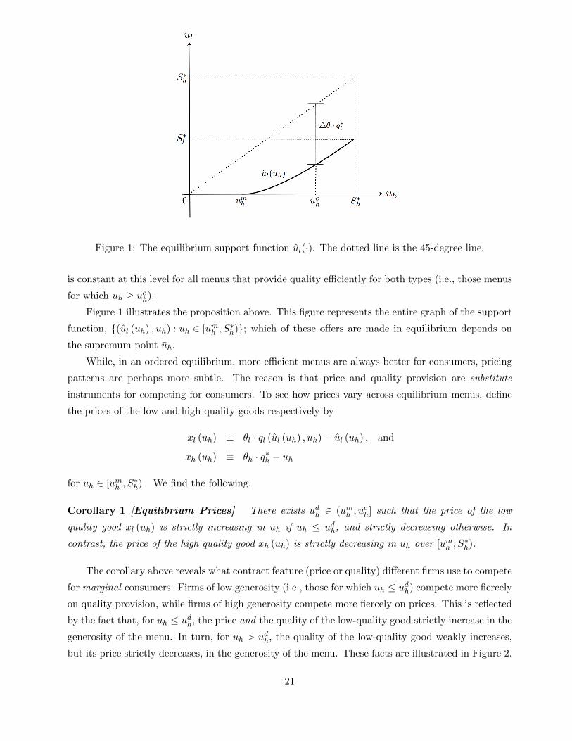
Figure 1: The equilibrium support function ul(·). The dotted line is the 45-degree line.

is constant at this level for all menus that provide quality efficiently for both types (i.e., those menus

for which uh ≥ uch).

Figure 1 illustrates the proposition above. This figure represents the entire graph of the support

function, (ul (uh) , uh) : uh ∈ [umh , S∗h); which of these offers are made in equilibrium depends on

the supremum point uh.

While, in an ordered equilibrium, more efficient menus are always better for consumers, pricing

patterns are perhaps more subtle. The reason is that price and quality provision are substitute

instruments for competing for consumers. To see how prices vary across equilibrium menus, define

the prices of the low and high quality goods respectively by

xl (uh) ≡ θl · ql (ul (uh) , uh)− ul (uh) , and

xh (uh) ≡ θh · q∗h − uh

for uh ∈ [umh , S∗h). We find the following.

Corollary 1 [Equilibrium Prices] There exists udh ∈ (umh , uch] such that the price of the low

quality good xl (uh) is strictly increasing in uh if uh ≤ udh, and strictly decreasing otherwise. In

contrast, the price of the high quality good xh (uh) is strictly decreasing in uh over [umh , S∗h).

The corollary above reveals what contract feature (price or quality) different firms use to compete

for marginal consumers. Firms of low generosity (i.e., those for which uh ≤ udh) compete more fiercely

on quality provision, while firms of high generosity compete more fiercely on prices. This is reflected

by the fact that, for uh ≤ udh, the price and the quality of the low-quality good strictly increase in the

generosity of the menu. In turn, for uh > udh, the quality of the low-quality good weakly increases,

but its price strictly decreases, in the generosity of the menu. These facts are illustrated in Figure 2.

21

Figure 2: The low-type quality schedule (full curve and left-side Y-axis)) and the low-type price

(dotted curve and right-side Y-axis) as a function of the generosity of the menu, uh.

The reason why the price of the low-quality good is initially increasing in the menu’s generosity

relates to the shape of the support function ul (·). Crucially, the support function ul (·) is convex

and has zero derivative at umh , the Mussa-Rosen indirect utility.17,18 This implies that, for low

values of uh, the low-type quality increases fast, while low-type payoffs ul (uh) increase slowly in

uh. Necessarily, therefore, the price of the low-quality good has to increase in uh, as dictated by

incentive compatibility. In turn, for high values of uh, quality provision to low types increases at a

lower rate than indirect utilities, implying that prices have to decrease in uh. Finally, that the price

of the high-quality good xh (uh) is decreasing follows straightforwardly because the high-type quality

remains fixed at its efficient level.

The next subsection studies how the distributions over menus (and its support) vary with the

degree of competition in the market. It shows that more competition leads to higher payoffs for

consumers and lower distortions in quality provision. Moreover, by varying the degree of competition

in the market, we span the entire spectrum of competitive intensity, from perfect competition to

17A simple intuition for why ul (·) is convex is as follows. As the generosity of the menu increases, so does the social

surplus generated by the low-type contract (as established in Proposition 2). This implies that, relative to high-types,

sales to low-types become increasingly attractive for firms (as the surplus to be shared with consumers from each sale

increases). Therefore, relative to high types, competition for low types get fiercer as uh increases. This is reflected in

the fact that as menus become more generous, the indirect utilities left to low-types increases faster in uh.18To get intuition on why u

l (uh) → 0 as uh → umh , consider the case where um

h > 0. By increasing the generosity of

the menu, the firm trades off profits per sale against the increased probability of a sale. For menus in a neighborhood

of the monopoly menu (0, umh ), increasing uh has only a second-order effect on the profitability of a sale, since um

h is an

interior maximizer of these profits. Increasing ul, however, leads to a first-order loss in profits per sale. Indifference

over menus therefore requires that the increase in high-type indirect utility be an order of magnitude larger than the

increase in low-type indirect utility for the same gain in the probability of a sale.

22

monopoly. Besides confirming standard intuitions, these results are instrumental for the distinctive

empirical predictions presented in subsection 3.7.

3.4 Comparative Statics

Before stating results, we introduce a mild regularity condition on the kernel Λ (y|v). This conditioncontrols for how sales functions change with the mass of firms v.

Condition 1 [VM] V-Monotonicity: The kernel ratio

R(y|v) ≡ Λ (y|v)Λ (0|v)

is strictly increasing in v for all y ∈ (0, 1].

Intuitively, this condition means that, relative to the least generous menu in the cross-section,

the proportional gains in sales from offering a contract whose indirect utility lies in some quantile

y > 0 increases with the mass of competing firms v. This captures the idea that, as the number

of competing firms increases, consumers are likely to have larger information sets, in which case

increasing the generosity of the offer has a larger impact on sales (relative to the monopolistic offer).

The monotonicity requirement of Condition VM is satisfied by the Generalized Burdett-Judd

matching model provided that, for any v > v, the sample size distribution Ω(v) dominates the

distribution Ω(v) in the likelihood-ratio order. In particular, this assumption is satisfied by the

Poisson-Burdett-Judd matching model (and, therefore, by the Butters model, which shares a similar

sales function). It is also satisfied by the Burdett-Mortensen matching model.

The next result establishes that, when competition increases, (i) firms more often offer menus

that lead to high indirect utilities for both consumer types, and (ii) the support of equilibrium

expands. As implied by Proposition 2, the mass of firms that offer inefficient qualities in equilibrium

decreases as competition gets fiercer.

Proposition 3 [Competition and Distortions: Comparative Statics] Assume that condition

VM holds, and denote by Fk and Fk (with supports Υk and Υk) the equilibrium distributions over

indirect utilities when the mass of firms is v and v, respectively. If v > v, then

1. Fk first-order stochastically dominates Fk, with Υk ⊆ Υk, for k ∈ l, h

2. the fraction of firms offering inefficient qualities is weakly lower for mass v: i.e., Fh(uch) ≤Fh(uch).

19

19If the IC-threshold uch belongs to support Υh = [um

h , uh], an increase in v can be shown to strictly decrease the

mass of firms offering inefficient qualities. See Proposition 5 below for necessary and sufficient conditions (in terms of

primitives) under which uh ≥ uch.

23

The proposition above captures changes in the degree of market competition by varying the mass

of firms, v. An alternative and intimately related notion of competition keeps v fixed, but varies the

level of frictions of the random matching technology. This is explored in the next remark.

Remark 4 [Frictions and Distortions] We say that the matching technology associated with the

kernel Λ (y|v) is less frictional than the matching technology associated with the kernel Λ (y|v) if forall y ∈ [0, 1],

Λ (y|v)Λ (0|v) ≥ Λ (y|v)

Λ (0|v).

This condition describes how sales functions change as the consumers’ information sets get larger (in

a probabilistic sense). In the Generalized Burdett-Judd model, the matching technology becomes less

frictional as the distribution of sample sizes increases in the sense of likelihood ratio dominance. In

the Poisson-Burdett-Judd model, the level of frictions is captured by the parameter β, which measures

how the mass of firms v impacts the average sample size observed by consumers. In the Butters model,

the level of frictions is captured by the parameter n, which is the number of consumers aware of the

menu of each firm.

Proposition 3 can be recast in terms of the degree of frictions of the matching technology: As the

matching technology becomes less frictional, e.g. when β or n increase, the distributions of indirect

utilities increase in the sense of first-order stochastic dominance, and the fraction of firms offering

efficient qualities increases.

3.5 Limiting Cases: Perfect Competition and Monopoly

The next proposition studies limiting properties of equilibria as the mass of firms in the market

converges to zero or infinity. These properties hold independently of Condition VM.

Proposition 4 [Competition and Distortions: Limiting Cases]

1. If limv→0R(1|v) = 1, then, as the mass of firms converges to zero, v → 0, the equilibrium

distribution over menus converges to a degenerate distribution centered at the monopolistic

(Mussa-Rosen) menu Mm. In particular, the fraction of firms offering inefficient menus is

one for small enough v.

2. If limv→∞R(y|v) = ∞ for all y ∈ (0, 1], then, as the mass of firms grows large, v → ∞,

the distribution over menus converges to a degenerate distribution centered at the competitive

(Bertrand) menu M∗. In particular, the fraction of firms offering efficient menus converges to

one.

The first part of Proposition 4 investigates the limit properties of equilibrium when v → 0. It

requires that the proportional gains in sales from offering the most generous contract in the cross-

section, relative to offering the least generous contract, converges to zero when the mass of competing

24

firms approaches zero. This is a weak condition satisfied by the matching technologies of Examples 2,

3 and 4. It also holds for the Generalized Burdett-Judd matching technology of Example 1 provided

that the collection of sample size distributions Ω(v) : v > 0 satisfies weak regularity conditions;20

the Poisson-Burdett-Judd matching technology is a particular case.

To understand the result, note that, as the mass of firms v approaches zero, the support of

h-type indirect utilities converges to umh , the Mussa-Rosen indirect utility. As a consequence, the

distribution over menus approaches a degenerate distribution centered at the monopolistic menu.

When the parameters of the price-discrimination problem dictate that qml = 0 (see equation (4)),

low types are excluded in the limit as v → 0.

The second part of Proposition 4 investigates the limit properties of equilibria when v → ∞. It

requires that the proportional gains on sales, relative to the least generous contract, from offering

a contract at any quantile y > 0, grows large as v → ∞. This condition is satisfied by the Gen-

eralized Burdett-Judd matching technology provided that weak regularity conditions are satisfied;21

the Poisson-Burdett-Judd matching technology is again a particular case. The condition is also

satisfied by the Butters matching technology. However, the condition is not satisfied by the Burdett-

Mortensen matching technology. Under this technology, the distribution over the menus that firms

offer converges to a non-degenerate distribution. It can be shown however that the distribution over

indirect utilities in the buyer-seller relationships that persist in the steady-state equilibrium indeed

converges to a degenerate distribution centered at the Bertrand menu.22

Importantly, Propositions 3 and 4 show how our model captures the entire spectrum of industry

competitiveness. When v is small, competition is weak, and we obtain the sensible prediction that

firms’ behavior is close to that of a firm with complete market power. When v is large, equilibria

approach the outcome of a perfectly competitive market.

Remark 5 [Vanishing Frictions] Similarly to Proposition 3, Proposition 4 can be recast in terms

of the degree of frictions of the matching technology. In the case of the Poisson-Burdett-Judd and

the Generalized Butters matching technologies (where frictions can be modeled parametrically), we

say that frictions vanish as β → ∞ and n → ∞, respectively. Accordingly, in the limit as frictions

vanish, the distribution over menus converges to a degenerate distribution centered at the competitive

(Bertrand) menu M∗.

20A sufficient condition is that the l1-limit of Ω(v) as v → 0 has support 0, 1.21A sufficient condition is that the l1-limit of Ω(v) as v → ∞ has support 2, 3, . . ..22The proof is available upon request. As described in Example 4, the Burdett-Mortensen model is a dynamic model

in which dynamic relationships persist only until the match exogenously terminates or the consumer receives a better

offer. Intuitively, as v becomes large, consumers receive offers very frequently in expectation and hence a relationship

in which the consumer earns a payoff bounded below the efficient surplus can be expected to last only a short while.

This explains why the distribution over payoffs earned by consumers in the relationships that have formed and not yet

broken in the steady state equilibrium of a Burdett-Mortensen economy converges to the Bertrand payoffs.

25

Before describing empirical implications, the next subsection discusses the important issue of

equilibrium uniqueness, and identifies the only possible source of equilibrium multiplicity in our

model.

3.6 Equilibrium Uniqueness

In a nutshell, the next proposition shows that, when the mass of firms v is small, the ordered

equilibrium is the unique equilibrium. In turn, when the mass of firms is large, there are equilibria

which are not ordered. As will be clear below, the uniqueness of equilibria crucially depends on

whether the incentive constraint ICh binds for all menus offered in the ordered equilibrium. In

the case of multiplicity, all equilibria exhibit the same distribution over contracts for each type of

consumer as the ordered equilibrium. Therefore, all equilibria induce the same marginal distribution

over indirect utilities to each type of consumer, and the same ex-ante profits for firms.

Proposition 5 [Incentive Constraints and Equilibrium Uniqueness] Assume that condition

VM holds, and that limv→0R(1|v) = 1 and limv→∞R(1|v) = ∞.23 Then there exists a threshold

vc > 0 on the mass of competing firms such that:

1. if v ≤ vc, the IC-threshold uch satisfies uch ≥ uh, and the downward incentive constraint (ICh)

is binding for all menus offered in the ordered equilibrium. In this case, the only equilibrium is

the ordered equilibrium.

2. if v > vc, the IC-threshold uch satisfies uch < uh, and the downward incentive constraint (ICh)

is slack for all menus in the ordered equilibrium with uh > uch, and binding for uh ≤ uch. In

this case, there exist multiple equilibria that differ only in the menus for which uh > uch (i.e.,

the efficient menus). However, all equilibria (including the non-ordered ones) lead to the same

marginal distributions over indirect utilities Fk(·), and the same ex-ante profits for firms.

The proof, contained in the Appendix, shows that in any equilibrium, when the mass of firms is

small (i.e., v ≤ vc), the support of utilities of type-k consumers, Υk, is contained in [umk , uck]. Using

the increasing differences property (see Lemma 2), we show that this implies that all equilibria are

equal to the ordered equilibrium.

In contrast, when the mass of firms is large (i.e., v > vc), some menus offered in the ordered

equilibrium exhibit non-binding incentive constraints. Consider such a menu (ul(uh), uh), in which

case uh ∈ (uch, uh]. For this menu, the profit function π(ul, uh) is locally modular, i.e. its cross-

partial derivative is zero. As a result, for some (small) ε > 0, both the menus (ul(uh − ε), uh) and

(ul(uh), uh − ε) are profit-maximizing for the firm. Based on the ordered equilibrium, we can thus

construct a non-ordered equilibrium by replacing the menus (ul(uh), uh) and (ul(uh − ε), uh − ε) by

23This is technical condition is satisfied by the matching technologies of Examples 1 2, 3 and 4.

26

their non-ordered counterparts (ul(uh− ε), uh) and (ul(uh), uh− ε). Proposition 5 confirms that this

is the unique source of multiplicity of equilibria in our economy.

Remark 6 [Frictions and Uniqueness of Equilibrium] The statements above can be recast in

terms of the degree of frictions of the matching technology. Namely, in the case of the Poisson-

Burdett-Judd and the Generalized Butters models, the uniqueness result of Proposition 5 holds if and

only if the friction parameters β and n are small enough.

3.7 Empirical Implications

Taken together, the results above deliver interesting empirical implications. To describe them, con-

sider a market where multi-product retailers offer two goods of different qualities, a low-quality (or

baseline) good and a high-quality good (superior version). Our first implication follows directly from

Proposition 2.

Empirical Implication 1 [Qualities and Profit Shares] Firms that offer baseline (low-quality)

goods of higher quality obtain a larger fraction of their profits from baseline goods.

Combining Corollary 1 with Propositions 2, 3 and 4 generates the following empirical implica-

tions.

Empirical Implication 2 [Qualities and Prices] There exists vd ∈ (0, vc] such that:

1. If competition is not too intense (i.e., v < vd), the price charged for the baseline good is an

increasing function of its quality.

2. If competition is not too intense (i.e., v < vd), the price of the baseline good is a decreasing

function of the price of the superior version.

3. If competition is sufficiently intense (i.e., v > vd), the price of the baseline good is a U-shaped

function of the price of the superior version.

To understand this implication, recall from Corollary 1 that the price charged for the baseline

good is increasing in the generosity of the menu if uh ≤ udh, and decreasing otherwise. In turn,

Propositions 3 and 4 imply that the equilibrium support of type-h indirect utilities, Υh, is contained

in the interval [umh , udh) if and only if v is small enough (i.e., v < vd). Accordingly, whenever

competition is not too intense, the price charged for the baseline good is an increasing function of

its quality, and a decreasing function of the price of the superior version. Notice by Proposition 5

that these facts hold independently of any equilibrium selection (as vd ≤ vc, which means that the

ordered equilibrium is the unique equilibrium).

27

When, in turn, competition is sufficiently intense (i.e., v > vd), the support of type-h indirect

utilities, Υh, is a superset of [umh , udh). Because, by Corollary 1, the baseline price is an inverse

U-shaped function of the menu’s generosity, it follows that the baseline price offered by a firm is a

U-shaped function of the price of the superior version. Notice by Proposition 5 that if v is too large

(i.e., v > vc ≥ vd), this result hinges on selecting the ordered equilibrium (as there is equilibrium

multiplicity for menus in the range uh > uch).

Perhaps unexpectedly, more competition may have price-increasing effects.

Empirical Implication 3 [Price-Increasing Competition] If competition is not too intense

(i.e., v < vd), more competition leads to higher prices for the baseline good (in the appropriate

probabilistic sense).24

Yet, consumers are better off, as qualities increase faster than prices, leading to higher indirect

utilities (in the appropriate probabilistic sense identified by Proposition 3). Finally, note by Propo-

sition 5 that this fact holds independently of any equilibrium selection (as the ordered equilibrium

is the unique equilibrium).

The empirical implications described above arise from the interplay between heterogeneity of

information about market offers and asymmetric information regarding consumer tastes. We hope

that these implications may by useful for empirical work trying to assess to what extent the market

power enjoyed by firms stems from heterogeneity of information or other sources (such as brand

preferences).

4 Extensions

The analysis so far assumed that consumer information is exogenous. This simplification was useful

to isolate the effects of competition on the firms’ pricing and quality provision. In this section, we

endogenize consumer information, and show that the main insights of our analysis naturally extend

to this more general environment.

The endogeneity of consumer information stems from two different sources. First, consumers

may invest in information acquisition, so as to learn the offers available in the market. Second, firms

may invest in advertising, so as to better inform consumers about their offers. The next subsections

show that we can easily incorporate information acquisition by consumers, or endogenous advertising

by firms, in our model of competitive nonlinear pricing.

24Formally, let us denote by Gl and Gl the equilibrium distributions over the prices of the low quality good offered

by firms when the mass of firms is v and v, respectively. Then, whenever v < v < vd, Gl first-order stochastically

dominates Gl.

28

4.1 Information Acquisition by Consumers

For simplicity, we consider the binary-type model studied in Section 3, and assume that consumer

information is generated by the Burdett-Judd random matching model of Example 1.

We model information acquisition by assuming that, after learning their willingness to pay for

quality, consumers can make investments that affect the size of their information sets (i.e., the

sample of firms they are aware of).25 If a consumer invests nothing, his sample size distribution

is Ω0 = ω0j : j = 0, 1, 2, . . ., where ω0

j > 0 is the probability of observing a sample of j firms.

The distribution Ω0 captures, in probabilistic terms, the information obtained spontaneously by

consumers about the offers available in the market. We assume that ω00 > 1

2 ; i.e., if a consumer

makes no investment, then he is more likely to observe no offer than one or more offers.

Investing in information acquisition shifts the consumer sample-size distribution according to

first-order stochastic dominance. Specifically, we assume that investing z ∈ [0, 1] generates a sample

size distribution Ωz = ωzj : j = 0, 1, 2, . . ., where

ωzj ≡ (1 + z) · ω0

j for j = 1, 2, . . . ,

and ωz0 ≡ 1−

j≥1 ω

zj . Accordingly, investments in information acquisition scale up the probability

of sample sizes weakly larger than one.

Let consumers with low and high types invest zl and zh in information acquisition. Denoting

by Λz (·) the sales kernel associated with the sample-size distribution Ωz, we can write the firms’

profit-maximization problem (in response to the cross-section cdf’s over indirect utilities Fl, Fh)as that of choosing a menu (ul, uh) to maximize

k=l,h

pk · Λzk (Fk(uk)) · (Sk(ul, uh)− uk) =

k=l,h

pk · (1 + zk) · Λ0 (Fk(uk)) · (Sk(ul, uh)− uk) ,

where the equality above follows from the formula for the Burdett-Judd kernel in Example 1. By

letting pk(zk) ≡ pk · (1 + zk), we can see that the firms’ problem when consumers invest (zl, zh) in

information acquisition is the same as if the mass of high and low types were pl(zl) and ph(zh), and

no information acquisition was possible.

It then follows from Proposition 1 that, for any profile of investments (zl, zh), there exists a

unique ordered equilibrium, where the masses of consumers of each type (pl, ph) are replaced by

the adjusted masses (pl(zl), ph(zh)). The effect of information acquisition by consumers is therefore

equivalent to a change in the masses of each consumer type. In particular, the equilibrium behavior

of firms satisfies the properties described in Proposition 2.

Of course, when information acquisition is endogenous, the firms’ choice of menus and the

consumers’ investment decisions are jointly determined. To describe the consumers’ investment

25De los Santos, Hortacsu and Wildenbeest (2012) provide empirical evidence that sample-size search, as considered

here, better explains consumer behavior than other modes of search (for example, sequential).

29

problem, let us assume that investing z in information acquisition costs ψ(z) to consumers, where

the cost function ψ(·) is continuously differentiable, strictly increasing and strictly convex, with

ψ(0) = ψ(0) = 0 and limz→1 ψ(z) = ∞ (which guarantees an interior solution). It is convenient to

denote by U1:jk the random variable defined as the highest realization out of j iid draws from each

distribution Fk, for k ∈ l, h. A consumer with type k ∈ l, h then chooses his investment in

information acquisition to maximize his payoff

∞

j=1

ωzj · E

U1:jk

− ψ(z) = (1 + z) ·

∞

j=1

ω0j · E

U1:jk

− ψ(z). (18)

An equilibrium with information acquisition is a triple (F , zl, zh) such that the firms’ choice of

menus and the consumers’ investment decision constitute mutual best responses.26

Since the marginal benefit of information acquisition is uniformly larger for high than for low

types, we must have zl < zh. As a consequence, the true and adjusted masses of consumer types

satisfyphpl

<ph(zh)

pl(zl).

This implies that, relative to baseline model of Section 2, consumer information acquisition makes

high types “over-represented” in equilibrium, i.e., firms behave as if high-type consumers were more

frequent relative to low types than as implied by their actual masses.

4.2 Advertising and Entry by Firms

The model analyzed in the previous sections took the mass of firms v as exogenous. An important

and realistic possibility is that the number of firms is endogenously determined. To make things

concrete, we will consider in this subsection the model of Butters (1977), described in Example 3.

Suppose now that launching an advertising campaign costs K dollars, and that there is free entry

among firms. Firms that do not advertise are not in the informational set of any consumers, and

therefore make zero profits. Accordingly, the decision to advertise (and pay the cost K) coincides

with the firms’ decision of entering the market.

Let πm be the profit of a monopolist; i.e., the profit generated when the monopoly offer is

accepted with probability one. Whenever the entry cost is smaller than the monopolist’s profit,

K ∈ (0,πm) , the market operates and our model uniquely determines the level of competition in

terms of the mass of firms v. Indeed, the mass of firms v (K) entering is then given by the zero-profit

condition

K = Λ (0|v (K)) · πm. (19)

26The existence of an equilibrium with information acquisition follows from the Kakutani fixed-point theorem. The

proof of this claim, which key step establishes that the firms’ and consumers’ payoffs satisfy the appropriate continuity

properties, is available upon request.

30

In words, firms enter until the cost of entry is equal to the benefit. Given that all equilibrium offers

yield the same expected profit, this benefit is equal to the expected profit generated by the monopoly

offer (which, recall, is itself offered in equilibrium). The existence of a unique v (K) is guaranteed

by the assumption that K ∈ (0,πm) and because, in the Butters model, Λ (0|v) is strictly decreasing

in v with Λ (0|0) = 1. The mass of entrants v (K) is then decreasing in K, while the distribution

over low-type quality is also decreasing in K in the sense of first-order stochastic dominance (see

Proposition 3).

The free-entry version of our model described above is appropriate to address a classic question,

raised originally in Butters (1977), regarding the efficient level of advertising/entry. Absent private

information on consumer preferences, Butters shows that the level of entry in the decentralized

equilibrium is efficient. A simple explanation (not given in Butters, but in later work such as Tirole

(1988, Section 7.3.2.1) and Stegeman (1991)) is as follows. Absent private information on preferences,

all equilibrium offers prescribe efficient qualities, and the social surplus generated by any sale is the

same. Because in equilibrium firms make the same profits from any offer in the equilibrium support,

we can analyze a firm’s entry decision assuming that it makes the monopoly offer (which belongs

to the equilibrium support). Recall that the monopoly offer only translates in sales if the offer is

received by an otherwise unserved consumer, and that in this offer the firm appropriates the full

social surplus. It then follows that the firms’ private gains from advertising coincide with the social

gains from advertising, in which case advertising/entry is efficient.

This observation no longer holds when consumer preferences are private, as studied in this

paper. Indeed, a planner able to choose the level of entry, but not the menus offered by firms,

will choose higher entry than the equilibrium level. To understand why, note that, as in the case of

complete information, we can study a firm’s entry decision as if this firm were to offer the monopolist

menu (as implied by the fact that all equilibrium menus lead to the same expected profits). To

highlight the novelty of our finding, assume that the monopolist menu is such that only high types

are served. Therefore, as under complete information, the monopolist menu gives to the firm the

full social surplus generated by this menu. It then follows that, for a firm that offers the monopolist

menu, the private gains from advertising coincide with the social gains from advertising, in which

case advertising/entry is efficient. However, recall from Proposition 2 that all other equilibrium

menus generate strictly more social surplus than the monopolist menu. As a consequence, there is

a wedge between the private and the social gains from entry/advertising for all firms other than

the ones offering the monopolist menu. As result, welfare will increase if the planner subsidizes

entry/advertising (even when firms are free to choose their menus once in market).27

27If the monopolist menu serves both low and high types, there is another effect strengthening the inefficiency

result described above. In this case, even the firm offering the monopolist menu makes an inefficient advertising/entry

decision. The reason is that this firm no longer appropriates the full surplus from the menu it offers, as high-type

consumers are endowed to informational rents. This effect is related to the work of Stegeman (1991), who considers a

31

5 Conclusion

This paper studied imperfect competition in price-quality schedules in a market with informational

frictions. On the one hand, consumers have private information about their willingness to pay for

quality. On the other, consumers are imperfectly informed about the offers in the market, which is

the source of firms’ market power. While firms are ex-ante identical, equilibrium menus are dispersed

and can be ranked in terms of the generosity of their contracts to all consumer types. Firms that offer

more generous menus provide more efficient qualities, and obtain a higher fraction of their profits from

the low-quality goods offered in their menus. As the market becomes more competitive, equilibrium

approaches the Bertrand outcome. At the other extreme, all offers are close to the monopolistic

menu when competition is sufficiently weak. As we vary the mass of firms in the market, or the

degree of informational frictions, we continuously span the entire spectrum of competitive intensity.

We build on the results above to deliver a number of empirical implications that can be useful

in assessing the source of market power enjoyed by firms. Namely, we show that, under appropriate

conditions, (i) firms that charge higher baseline prices offer higher baseline quality, (ii) firms that

charge smaller baseline prices charge higher prices for the superior version of the product, and that

(iii) a decrease in the degree of information frictions generates higher prices for the baseline good.

The equilibrium characterization described above proceeded under the assumption of two con-

sumer types (with no restrictions on the probability distribution). In Appendix B, we extend our

characterization to the case of a continuum of types with a uniform distribution, and show that

our main insights remain true. The chief difficulty for analyzing other specifications stems from the

requirement that implementable quality schedules be monotonic in consumer types. It is difficult

to identify conditions on primitives that guarantee monotonicity in more general settings (where a

closed-form description of equilibrium is not available). To ascertain the robustness of our findings,

we have numerically calculated equilibria for the discrete-type case with various number of types,

and different distributions over consumer types. These numerical results indicate that the findings

of this paper are robust to other distributions of consumer preferences.

There are several interesting directions for further research. First, for the sake of tractability,

we have assumed that firms’ capacities are unconstrained, so they are able to fill all orders. Ca-

pacity constraints raise the possibility that those firms offering the most generous menus sell out, a

possibility that consumers should in turn anticipate. An examination of these “congestion effects”

seems difficult but worthwhile.

Second, we assumed that consumers observe the entire menu of qualities offered by each firm.

In practice, consumers may fail to consider all of the options that a firm offers; i.e., information

homogeneous good model where consumers have private information as to their reservation values. Stegeman too finds

that the competitive level of entry is inefficiently low, which can be attributed to the fact that the least generous (i.e.,

monopoly) offer in his model leaves positive surplus to the consumer.

32

imperfections may pertain also to a consumer’s ability to observe the entire menu. This possibility

has been explicitly recognized in empirical work (e.g., Sovinsky Goeree (2008)). In theoretical work,

Villas-Boas (2004) studies a monopolist whose consumers may (randomly) observe only the option

designed for the high or low type; extending the analysis to a competitive setting raises additional

challenges.

Third, one may hope to introduce additional dimensions to consumer preferences, such as brand

preferences, to bring the setting closer to the random utility models popular in empirical work

(for instance, suppose that, in addition to the payoffs specified in the model, consumers receive an

additional, continuously distributed, “shock” ε to their payoffs from purchasing from each seller).

We expect that our main qualitative insights are robust to this possibility. More broadly, our model

offers a useful theoretical benchmark against which models of imperfect competition with brand

preferences can be compared.

Finally, while we focused on sales of goods with variable quality, our results extend to other

contexts where information heterogeneity makes sense. A natural application, for instance, is to labor

markets where workers have private information about their productivities, and are heterogeneously

informed about the job offers available in the market. Contracts might pay wages based on the

worker’s output. In such settings, our results indicate dispersion over offers, with firms endogenously

segmenting themselves relative to (i) the indirect utility left to all worker types, (ii) the efficiency of

effort provision induced by their contracts, and (iii) the share of surplus obtained from workers with

different productivity levels.

References

[1] Armstrong, M. and Vickers, J., 2001. “Competitive Price Discrimination.” Rand Journal of

Economics, 32, 579-605.

[2] Berry, S., J. Levinsohn and A. Pakes, 1995. “Automobile Prices in Market Equilibrium.” Econo-

metrica, 63, 841-890.

[3] Bertrand J., 1883. “Theorie Mathematique de la Richesse Sociale.” Journal des Savants, 499-

508.

[4] Billingsley, P., 1995. Probability and Measure. New York: Willey Series in Probability and

Mathematical Statistics.

[5] Borenstein, S., 1985. “Price discrimination in free-entry markets.” RAND Journal of Economics,

16, 380-397.

33

[6] Borenstein, S. and N. Rose, 1994. “Competition and price dispersion in the U.S. airline industry.”

Journal of Political Economy, 102, 653-683.

[7] Butters, G., 1977. “Equilibrium Distributions of Sales and Advertising Prices.” The Review of

Economic Studies, 44, 465-491.

[8] Burdett, K., and Mortensen, D., 1998. “Wage Differentials, Employer Size, and Unemployment.”

International Economic Review, 39, 257-273.

[9] Burdett, K., and Judd, D., 1983. “Equilibrium Price Dispersion.” Econometrica, 51, 955-970.

[10] Calzolari, G., and V. Denicolo, 2013. “Competition with Exclusive Contracts and Market-Share

Discounts.” American Economic Review (forthcoming).

[11] Champsaur, P. and J.-C. Rochet, 1989. “Multi-product duopolists”. Econometrica, 57, 533–557.

[12] Clarke, F., 2013. Functional Analysis, Calculus of Variation and Optimal Control. London:

Springer.

[13] De los Santos, B., A. Hortacsu and M. Wildenbeest, 2012. “Testing Models of Consumer Search

Using Data on Web Browsing and Purchasing Behavior.” American Economic Review, 102, pp.

2955–2980.

[14] Diamond, P., 1971. “A Model of Price Adjustment.” Journal of Economic Theory, 3, 156-168

[15] Draganska, M., and D. Klapper (2011), “Choice Set Heterogeneity and The Role of Advertising:

An Analysis with Micro and Macro Data.” Journal of Marketing Research, 2011, 48, 653-669.

[16] Eeckhout, J., and P. Kircher, 2010. “Sorting versus Screening: Search Frictions and Competing

Mechanisms.” Journal of Economic Theory, 145, 1354-1385.

[17] Ellison, G., 2005. “A Model of Add-on Pricing.” Quarterly Journal of Economics, 120, 585-367.

[18] Faig, M. and B. Jerez, 2005. “A Theory of Commerce.” Journal of Economic Theory, 122, 60-99.

[19] Goldman, M., H. Leland, and D. Sibley. 1984. “Optimal Nonuniform Pricing.” Review of Eco-

nomic Studies, 51, 305-320.

[20] Grossman, G. M. and C. Shapiro, 1984. “Informative Advertising with Differentiated Products.”

Review of Economic Studies, 51, 63-81.

[21] Guerrieri, V., Shimer, R. and Wright, R., 2010. “Equilibrium Price Dispersion.” Econometrica,

78, 1823-1862.

34

[22] Inderst, R., 2001. “Screening in a Matching Market.” Review of Economic Studies, 2001, 68,

849-868.

[23] Inderst, R., 2004. “Contractual Distortions in a (Labor) Market with Frictions.” Journal of

Economic Theory, 116, 155-176.

[24] Ivaldi, M. and D. Martimort, 1994. “Competition under nonlinear pricing.” Annales d’Economie

et de Statistique, 34, 71–114.

[25] Katz, M.L., 1984. “Price Discrimination and Monopolist Competition.” Econometrica, 52,

1453-1471.

[26] McAfee, P., 1993. “Mechanism Design by Competing Sellers.” Econometrica, 78, 1823-1862.

[27] Maskin, E., and Riley, J., 1984. “Monopoly with Incomplete Information,” Rand Journal of

Economics, 15, 171-196.

[28] Moen, A. and Rosen, A., 2011. “Incentives in Competitive Search Equilibrium.” Review of

Economic Studies, 98, 733-761.

[29] Mussa, M. and Rosen S., 1978. “Monopoly and Product Quality.” Journal of Economic The-

ory,18, 301-317.

[30] Pai, M., 2013. “Competing Auctioneers.” Working Paper.

[31] Peters, M., 1997. “A Competitive Distribution of Auctions.” Review of Economic Studies, 64,

97-123.

[32] Peters, M., 2012. “Non-Contractible Heterogeneity in Directed Search.” Econometrica, 78,

1173–1200.

[33] Peters, M., and S. Severinov, 1996. “Competition among Sellers Who Offer Auctions Instead of

Prices.” Journal of Economic Theory, 75, 141-179.

[34] Petrongolo, B. and C. Pissarides, 2001. “Looking at the Black Box: A Survey of the Matching

Function.” Journal of Economic Literature, 39, 390-431.

[35] Rochet, J.C., and Stole, L., 1997. “Competitive Nonlinear Pricing.” Working paper.

[36] Rochet, J.C., and Stole, L., 2002. “Nonlinear Pricing with Random Participation.” The Review

of Economic Studies, 69, 2002, 277-311.

[37] Salop, S., and J. Stiglitz, 1977. “Bargains and Rip-Offs: A Model of Monopolistically Competi-

tive Price Discrimination.” Review of Economic Studies, 44, 493-510.

35

[38] Sovinsky Goeree, M., 2008. “Limited Information and Advertising in the U.S. Personal Com-

puter Industry.” Econometrica, 76, 1017-1074.

[39] Spulber, D., 1989. “Product variety and competitive discounts.” Journal of Economic Theory,

48, 510–525.

[40] Stegeman, M., 1991, “Advertising in Competitive Markets.” American Economic Review, 81,

pp. 210-223.

[41] Stole, L., 1991. “Mechanism design and common agency”. Working Paper.

[42] Stole, L., 1995. “Nonlinear pricing and oligopoly.” Journal of Economics & Management Strat-

egy, 4, 529– 562.

[43] Stole, L., 2007. “Price Discrimination and Competition.” In: Handbook of Industrial Organiza-

tion, vol. 3 (eds. M. Armstrong and R. Porter) North-Holland.

[44] Tirole, J., 1988. The Theory of Industrial Organization. The MIT Press.

[45] Varian, H., 1980. “A Model of Sales.” American Economic Review, 70, 651-659.

[46] Verboven, F., 1999. “International price discrimination in the European car market.” RAND

Journal of Economics, 27, 240–268.

[47] Villas-Boas, M., 2004. “Communication Strategies and Product Line Design.” Marketing Sci-

ence, 23, 304-316.

[48] Wilson, R., 1993. Nonlinear Pricing. Oxford Univ. Press, Oxford, UK.

[49] Yang, H., and Ye, L., 2008. “Nonlinear pricing, market coverage and competition.” Theoretical

Economics, 3, 123-153.

36

Online Appendix - Not for Publication

6 Appendix A: Proofs

Throughout, we economize notation by suppressing the dependence of Φ (uk|Fk, v, pk) on (Fk, v, pk)

for each k ∈ l, h; we simply write Φk (uk) = Φ (uk|Fk, v, pk).

Proof of Lemma 1. If the low type is offered the quality ql, then payoffs must satisfy ICh, i.e.,

uh ≥ ul +∆θql. (20)

On the other hand, IC l requires that

ul ≥ ul −∆θqh. (21)

The firm would like to make its offer as efficient as possible subject to the payoffs it delivers to the

consumer.

If uh−ul < ∆l ≡ ∆θq∗l , then offering the efficient quality q∗l for the low type is inconsistent with

(20), and the firm does best to choose the highest possible value. That is, the firm chooses quality

ql (ul, uh) which satisfies (20) with equality, or

ql (ul, uh) ≡uh − ul∆θ

.

If uh − ul ≥ ∆l, then the constraint (20) does not bind, and the firm chooses low-type quality

efficiently: ql (ul, uh) ≡ q∗l . Similarly, let ∆h ≡ ∆θq∗h. If uh − ul > ∆h, then asking the quality q∗hfor the high type violates (21), and so the best the firm can do is to choose qh (ul, uh) defined by

qh (ul, uh) ≡uh − ul∆θ

.

If uh − ul < ∆h, the firm offers the high-type an efficient quality: qh (ul, uh) ≡ q∗h. Q.E.D.

Proof of Lemma 2. To see this claim, note that πul, u2h

− π

ul, u1h

equals

Φl (ul)Sl

ul, u2h

− Sl

ul, u1h

+Φh

u2h

− Φh

u1h

Sh

ul, u2h

− u2h

+Φh

u1h

Sh

ul, u2h

− u2h

−Sh

ul, u1h

− u1h

.

(22)

The cross-partial ∂2

∂ul∂uhSl (ul, uh) is positive if uh−ul < ∆θq∗l and zero otherwise. Thus the first line

of (22) is strictly increasing over ul such that u1h − ul ≤ ∆θq∗l and constant otherwise. The function

Sh

·, u2h

is strictly increasing if qh

ul, u2h

> q∗h and constant otherwise. Thus the second line in

(22) is increasing in ul. The cross-partial ∂2

∂ul∂uhSh (ul, uh) is positive if uh − ul > ∆θq∗h and is zero

37

otherwise. Thus the third term is strictly increasing over ul such that u2h − ul ≥ ∆θq∗h and constant

otherwise. These arguments imply the result. Q.E.D.

Proof of Lemma 3. We divide the proof in five steps.

Step 1 No mass points in the distribution of high-type offers.

We begin by showing that Fh has no mass points. Assume towards a contradiction there is an

atom of firms offering uh.

We first show that, if a firm makes an equilibrium offer (ul, uh), for some value ul, then

Sh(ul, uh)−uh > 0. Suppose not. Then it must be that Sl(ul, uh)−ul ≤ 0 (in case Sh(ul, uh)−uh ≤ 0

and Sl(ul, uh) − ul > 0, offering only the option designed for the low type improves the seller’s ex-

pected profit because high types accept such an offer with positive probability). Hence, π (ul, uh) ≤ 0.

This contradicts seller optimization. Indeed, the seller could offer a menu which yields the Mussa

and Rosen utilities (uml , umh ) and obtain a payoff at least as large as (S∗h − umh )Φh (0) > 0.

Next, notice that Sl(ul, uh) − ul ≥ 0. If not, the seller can profit by offering the menu

(ql, xl) = (0, 0) and (qh, xh) = (q∗h, θhq∗h − uh). Irrespective of whether the low type finds it in-

centive compatible to choose the option (0, 0), the seller is guaranteed an expected profit at least as

high as under the original menu.

These two observations imply that π (ul + ε, uh + ε) > π (ul, uh) for ε > 0 sufficiently small,

contradicting the optimality of (ul, uh). To see this, note that π (ul + ε, uh + ε) must be bounded

below by

π (ul, uh)− ε [Φh (uh + ε) + Φl (ul + ε)]

+ (Sh(ul, uh)− uh − ε) [Φh (uh + ε)− Φh (uh)] ,

Since Φh (uh + ε) − Φh (uh) is bounded above zero as ε 0, and since Sh(ul, uh) − uh > 0, the

expression above is greater than π (ul, uh) whenever ε is sufficiently small.

Step 2 No mass points in the distribution of low-type offers.

First, we show that there are no mass points in Fl at any ul > 0. Suppose towards a contradiction

that Fl has a mass point at some ul > 0. Take a firm that offers (ul, uh) . Since, as reasoned above,

Sl(ul, uh)− ul ≥ 0, we can consider two cases.

Case 1: Sl(ul, uh)− ul > 0.

As noted in Step 1, the expected profit conditional on selling to a high type must also be positive.

Notice that in this case π (ul + ε, uh + ε) is bounded below by

π (ul, uh)− ε [Φh (uh + ε) + Φl (ul + ε)]

+ (Sl(ul, uh)− ul − ε) (Φl (ul + ε)− Φl (ul)) .

38

Since Φl has a mass point at ul, and since Sl(ul, uh)− ul > 0, the expression above is strictly greater

than π (ul, uh) for ε > 0 sufficiently small.

Case 2: Sl(ul, uh)−ul = 0. Let (ql, xl) , (qh, xh) = (ql (ul, uh) , xl (ul, uh)) , (qh (ul, uh) , xh (ul, uh))be the menu offered by the firm. Consider a deviation to the menu (ql, xl + ε) , (qh, xh) for some

ε ∈ (0, ul) . This menu generates the same expected profits from high types and is accepted with

positive probability by low types. Moreover, since Sh(ul, uh)− uh > 0 (see Step 1), the seller makes

positive profits whether a low-type buyer chooses the option (ql, xl + ε) or (qh, xh). That is, expected

profits from low types are strictly positive under the deviating offer.

Finally, we show that there can be no mass point in Fl at zero. Assume towards a contradiction

that Fl(0) > 0. From Step 1 (i.e., since there are no mass points in the distribution of high-type

offers), menus (ul, uh) ∈ 0× [ε,∞) are then offered with positive probability. It is easy to see that

there is χ > 0 such that Sl (0, uh) > χ for all uh ∈ [ε,∞). Therefore, for small η > 0 the difference

π (η, uh)− π (0, uh) is

(Φl (η)− Φl (0)) [Sl (η, uh)− η]

−Φl (0) (Sl (0, uh)− Sl (η, uh)− η) .(23)

We can take η∗ such that η ∈ (0, η∗) implies that the first line of (23) is at least (Φl (0+)− Φl (0))χ2

>

0. Moreover, the second line of (23) converges to 0 as η 0, which shows a profitable deviation.

Step 3 The supports Υk are intervals.

Suppose for a contradiction that one or both of the supports are disconnected sets. Assume that

Υl is disconnected. Then there are ul and ul in Υl with ul < ul such that (ul, ul )∩Υl = ∅. Consider

values uh and uh such that (ul, uh) and (ul , u

h) are optimal. From Steps 1 and 2 and Lemma 2 we

may assume that Φl (ul) = Φl (ul ), Φh (uh) = Φh (uh) and uh ≤ uh.

If uh < uh then there is ε > 0 for which π (ul − ε, uh − ε) > π (ul , uh) . Thus assume that

uh = uh. For any ε ∈ (0, ul − ul), optimality requires π (ul − ε, uh) ≤ π (ul , uh). This implies that

qh (ul , uh) > q∗h, i.e. ICl binds. Thus ∂2Sh(ul,uh)

∂u2l

< 0 at (ul , uh) , which implies (using Φl (ul) =

Φl (ul )) that π (λul + (1− λ)ul , uh) > λπ (ul, u

h) + (1− λ)π (ul , u

h) for λ ∈ (0, 1). Hence, (ul , u

h)

is not optimal. The proof that Υh is connected is analogous and omitted.

Step 4 The minimum of the supports Υl and Υh are, respectively, uml = 0 and umh .

Let ul and uh be the minimum of the supports of Υl and Υh respectively. It follows from Steps

1 and 2 and from Lemma 2 that (ul, uh) is an optimal menu. IR requires ul ≥ 0, and we next show

that ul = 0. To see this, suppose that ul > 0 and note that uh ≥ ul. Since Φl (0) = Φl (ul) and

Φh (uh − ul) = Φh (uh) , we have π (0, uh − ul) > π (ul, uh) , a contradiction. Hence indeed ul = 0

and so uh ≥ 0 maximizes

Φl (0)Sl (0, uh) + Φh (0) (Sh (0, uh)− uh) . (24)

39

Since umh is the only maximizer of (24), the claim follows. We have thus established that, for each

k ∈ l, h, the support Υk is equal to [umk , uk], where uk > umk .

Step 5 Fl and Fh are absolutely continuous.

We will show that Fh is Lipschitz continuous (the proof that Fl is absolutely continuous is

analogous and omitted). Notice that from 2. in Assumption 1 it suffices to show that Φh is Lipschitz

continuous. For that, it is enough to show that there are positive values K and δ such that, for all

uh ∈ Υh and all ε ∈ (0, δ), Φh (uh + ε)− Φh (uh) < Kε .

First, we claim that we may find a constant Sh > 0 such that we have Sh (ul, uh) − uh ≥ Sh

for every optimal menu (ul, uh) . The claim follows by the same logic as in Step 1. If the claim

does not hold, we may find a sequence of optimal menus (unl , unh) such that Sh (unl , u

nh) − unh ≤ 1

n .

Taking a subsequence if necessary, assume that (unl , unh) → (u∗l , u

∗h) . By the continuity of Φk (Steps

1 and 2) and the continuity of Sk (for k ∈ l, h) we conclude that (u∗l , u∗h) is optimal and that

Sh (u∗l , u∗h)− u∗h = 0. However, we showed in Step 1 that such a menu cannot be optimal.

Next, let δ > 0 and define ξh := sup(ul,uh)∈[0,ul]×[umh ,uh+δ]:uh≥ul

∂Sh(ul,uh)∂uh

. Take any equilib-

rium menu (ul, uh) ∈ Υl ×Υh. Notice that, for ε ∈ (0, δ), π (ul, uh + ε) is

Φl (ul) [Sl(ul, uh + ε)− ul] + Φh (uh + ε) [Sh(ul, uh + ε)− uh − ε]

≥

Φl (ul) [Sl(ul, uh)− ul] + Φh (uh) [Sh(ul, uh)− uh]

−Φh (uh) (ξh + 1) ε+ [Φh (uh + ε)− Φh (uh)] (Sh − (ξh + 1) ε)

.

Since π (ul, uh + ε) ≤ π (ul, uh) we have:

Φh (uh + ε)− Φh (uh)

ε≤ Φh (uh) (ξh + 1)

Sh − (ξh + 1) ε<

Φh (uh) (ξh + 1)

Sh − (ξh + 1) δ.

Since Part 3 of Assumption 1 implies Φh (uh) < +∞, it is then easy to see that our claim holds

provided K is sufficiently large and δ sufficiently small. Q.E.D.

Proof of Proposition 1. As explained in the proof sketch contained in the text, we divide the

proof in three steps.

Step 1 Constructing the support function.

Necessity of (7) and (8). We first show that Φh (·) and Φl (·) are continuously differentiable.

By Assumption 1.2, this implies that each Fk (uk) is continuously differentiable as well. Hence, the

firm’s profits π (ul, uh) as defined by (6) are continuously differentiable, with first-order conditions

given by (7) and (8).

40

We focus on the claim that Φh (·) is continuously differentiable, as the case of Φl (·) is analogous.Let uh ∈ Υh and suppose that ul = ul (uh), so that (ul, uh) is an optimal menu. Note that for any

ε ∈ R, we have

Φl (ul) [Sl(ul, uh + ε)− ul] + Φh (uh + ε) [Sh(ul, uh + ε)− uh − ε]

= Φl (ul) [Sl(ul, uh)− ul] + Φh (uh) [Sh(ul, uh)− uh]

+Φl (ul) [Sl(ul, uh + ε)− Sl(ul, uh)] + Φh (uh) [Sh(ul, uh + ε)− ε− Sh(ul, uh)]

+ [Φh (uh + ε)− Φh (uh)] [Sh(ul, uh + ε)− uh − ε] .

Since π (ul, uh) ≥ π (ul, uh + ε), we have

[Φh (uh + ε)− Φh (uh)] [Sh(ul, uh + ε)− uh − ε]

≤ Φl (ul) [Sl(ul, uh)− Sl(ul, uh + ε)] + Φh (uh) [Sh(ul, uh)− Sh(ul, uh + ε) + ε] .

Next, for any ε ∈ R such that uh + ε ∈ Υh, let ul,ε = ul (uh + ε). Thus, we have

Φl (ul,ε) [Sl(ul,ε, uh + ε)− ul,ε] + Φh (uh + ε) [Sh(ul,ε, uh + ε)− uh − ε]

= Φl (ul,ε) [Sl(ul,ε, uh)− ul,ε] + Φh (uh) [Sh(ul,ε, uh)− uh]

+Φl (ul,ε) [Sl(ul,ε, uh + ε)− Sl(ul,ε, uh)] + Φh (uh) [Sh(ul,ε, uh + ε)− ε− Sh(ul,ε, uh)]

+ [Φh (uh + ε)− Φh (uh)] [Sh(ul,ε, uh + ε)− uh − ε] .

Since π (ul,ε, uh + ε) ≥ π(ul,ε, uh), we have

[Φh (uh + ε)− Φh (uh)] [Sh(ul,ε, uh + ε)− uh − ε]

≥ Φl (ul,ε) [Sl(ul,ε, uh)− Sl(ul,ε, uh + ε)] + Φh (uh) [Sh(ul,ε, uh)− Sh(ul,ε, uh + ε) + ε] .

For the right derivative we now consider ε > 0 (the case of the left derivative is analogous). For any

ε sufficiently small, we have Sh(ul, uh + ε) − uh − ε > 0 (to see this, consider the argument in Step

1 of the proof of Lemma 3). For all such ε, we have

Φl (ul,ε) [Sl(ul,ε, uh)− Sl(ul,ε, uh + ε)]

+Φh (uh) [Sh(ul,ε, uh)− Sh(ul,ε, uh + ε) + ε]

ε [Sh(ul,ε, uh + ε)− uh − ε]≤ Φh (uh + ε)− Φh (uh)

ε

≤

Φl (ul) [Sl(ul, uh)− Sl(ul, uh + ε)]

+Φh (uh) [Sh(ul, uh)− Sh(ul, uh + ε) + ε]

ε [Sh(ul, uh + ε)− uh − ε].

Next, note that ul (·) must be continuous by Lemma 3, since each Fk is continuous and Fl (ul (uh)) =

Fh (uh) for all uh. Hence ul,ε ul as ε 0, implying that the right derivative of Φh (uh) is equal

to−Φl (ul)

∂Sl(ul,uh)∂uh

+ Φh (uh)1− ∂Sh(ul,uh)

∂uh

Sh(ul, uh)− uh

41

The left derivative can similarly be shown to take the same value, i.e., Φh (uh) is differentiable at uh.

Using our assumption that ICl is slack, we can thus conclude that

Φh (uh) =

−Φl (ul)∂Sl(ul,uh)

∂uh+ Φh (uh)

S∗h − uh

(25)

Φl (ul) =

Φl (ul)1− ∂Sl(ul,uh)

∂ul

Sl(ul, uh)− ul. (26)

Recall that uh < S∗h by Lemma 3. Moreover, we must have Sl(ul, uh) − ul > 0 whenever uh > 0

(this follows from the argument in Step 2, Case 2 of Lemma 3). Hence, both derivatives are finite

over uh ∈ (umh , uh).

Verifying (15). Next we want to verify that ul (uh) is differentiable with derivative given by

(15). Indeed, note from (26) that Φl (ul) is strictly positive at ul = ul (uh) for any uh ∈ (umh , uh).

Thus, by the implicit function theorem, ul (uh) =Φ

h(uh)Φ

l(ul(uh)), which is precisely (15).

Existence and properties of solution to ODE. As described in the main text, (7), (8) and

(15) imply that the support function ul must satisfy

ul(uh) = h (ul (uh) , uh) , (27)

where

h (ul, uh) =Sl (ul, uh)− ul

S∗h − uh

·1− pl

ph∂Sl∂uh

(ul, uh)

1− ∂Sl∂ul

(ul, uh), (28)

and where we impose the boundary condition ul (umh ) = 0. We now show that there exists a unique

solution ul (·) on [umh , S∗h).

For any ε ∈ (0, S∗h), the function h (·, ·) is Lipschitz continuous on

Γ (ε) ≡ (ul, uh) ∈ [0, S∗l ]× [umh , S∗

h − ε) : ul < uh .

Hence, by the Picard-Lindelof theorem, for any ε ∈ (0, S∗h), and for any (ul, uh) in the interior of

Γ (ε), there is a unique local solution to ul (uh) = h (ul (uh) , uh). Local uniqueness will extend to

global uniqueness, guaranteeing that the equilibrium we construct is the only ordered equilibrium.

Now consider ul (uh) = h (ul (uh) , uh) with initial condition ul (umh ) = 0 and note the existence

of η > 0 such that a unique solution exists on [umh , umh + η] where (ul (uh) , uh) remains in Γ (0). We

now show that h (ul (uh) , uh) remains bounded and that (ul (uh) , uh) remains in Γ (0) also as uh

increases to S∗h, implying the existence of a global solution to ul (uh) = h (ul (uh) , uh) on [umh , S∗

h).

We further show that h (ul (uh) , uh) remains strictly positive on [umh , S∗h) (as explained in the main

text, this ensures that the equilibrium we construct is ordered). The problem should be considered

for two regions of uh: we show that there exists a value uch ∈ (umh , S∗h) such that uch− ul (uch) = q∗l ∆θ

42

and such that uh − ul (uh) < q∗l ∆θ for uh ∈ [umh , uch). We then show that uh − ul (uh) > q∗l ∆θ for

uh > uch.

First, we show that, for uh > umh , provided uh− ul (uh) remains below q∗l ∆θ, then h (ul (uh) , uh)

remains in (0, 1). First, note that Sl (ul (uh) , uh) − ul (uh) remains strictly positive: this follows

because dduh

[Sl (ul (uh) , uh)− ul (uh)] > 0 whenever Sl (ul (uh) , uh)− ul (uh) is sufficiently close to

zero. Second, h (ul (uh) , uh) remains below 1 because

S∗h − uh − (Sl (ul (uh) , uh)− ul (uh))

= θhq∗h − ϕ (q∗h)− (θlql (ul (uh) , uh)− ϕ (ql (ul (uh) , uh)))− ql (ul (uh) , uh)∆θ

= θhq∗h − ϕ (q∗h)− (θhql (ul (uh) , uh)− ϕ (ql (ul (uh) , uh)))

> 0 (29)

and plph

∂Sl∂uh

(ul (uh) , uh) > ∂Sl∂ul

(ul (uh) , uh) whenever uh − ul (uh) < q∗l ∆θ. Finally, to check that

h (ul (uh) , uh) remains strictly positive, we note that plph

∂Sl∂uh

(ul (uh) , uh) < 1 provided uh− ul (uh) >

umh , which is guaranteed in turn by the initial condition and that h (ul (uh) , uh) remains less than 1.

We now verify the existence of uch ∈ (umh , S∗h) for which uch − ul (uch) = q∗l ∆θ. Suppose that

there is no such value uch. Then the equalities in (29) must continue to hold for all uh ∈ (umh , S∗h).

Since these expressions are bounded above zero, we must have Sl (ul (uh) , uh) − ul (uh) < 0 as uh

approaches S∗h, contradicting the observation in the previous claim.

Next, consider extending the solution to uh ∈ (uch, S∗h). It is easily checked that ul (uh) =

S∗l − α (S∗

h − uh) with α =S∗l −ul(uc

h)S∗h−uc

h∈ (0, 1) satisfies ul (uh) = h (ul (uh) , uh) and remains in Γ (0)

(that ul (uh) remains below S∗l follows because S∗

l − ul (uh) = α (S∗h − uh) > 0).

The extension of the solution to uh ∈ (uch, S∗h) completes the construction of the support function.

We can then check that the incentive constraint ICl (i.e., (21)) is globally satisfied, as we do next.

The Incentive Constraint ICl is globally satisfied. The above showed that there is uch ∈(umh , S∗

h) for which uh − ul(uh) < ∆θq∗l for all uh < uch. For uh ∈ [uch, S∗h) we have

uh − ul(uh) = (uh − S∗l ) + α (S∗

h − uh) . (30)

Notice that the derivative of the RHS of (30) w.r.t. uh is 1−α > 0. Hence (30) achieves its maximum

at uh = S∗h and its maximum is given by

S∗h − S∗

l = ∆θq∗l +

ˆ q∗h

q∗l

θh − ϕ(q)

dq < ∆θq∗h.

Thus we conclude that uh − ul(uh) ∈ (∆θq∗l ,∆θq∗h) for all uh ∈ (uch, S∗h). Therefore, the incentive

constraint (21) does not bind along the curve (ul (uh) , uh) .

Step 2 Solving for the distribution F .

43

As noted above (see Step 4 in the proof of Lemma 3), the least generous equilibrium menu must

be (uml , umh ) . Moreover, in equilibrium, all offers must yield the same expected profit

π∗ :=

k=l,h

pk · Λ (0|v) · (Sk(uml , umh )− umk ) .

Next, observe that there is a value uh > umh which solves

Λ (1|v)

k=l,h

pk · (Sk(ul(uh), uh)− uk(uh)) = π∗

The existence of such uh is guaranteed by the intermediate value theorem, since Λ(1|v)Λ(0|v) ∈ (1,∞) and

since limuh↑S∗h[Sl(ul (uh) , uh)− ul (uh)] = limuh↑S∗

h[S∗

h − uh] = 0.

Condition (13) is then simply the requirement that

Λ (Fh(uh)|v)

k=l,h

pk · (Sk(ul(uh), uh)− uk(uh)) = π∗

for uh ∈ [umh , uh] where Fh(uh) = 1. Note then that dduh

k=l,h pk · (Sk(ul(uh), uh)− uk(uh))

< 0

on (umh , uh). This follows because dduh

[uh − ul(uh)] > 0 and uh − ul(uh) > umh , and because

ul(uh) > 0. Hence, Assumption 1.1 and 1.2 imply that Fh is uniquely defined by (13) and is

increasing and differentiable on (umh , uh). Finally, Fl is uniquely defined by Fl(ul(uh)) = Fh(uh).

Step 3 Verifying the optimality of equilibrium menus.

It now remains to check that firms have no incentive to deviate from the putative equilibrium

strategies. By construction, all menus (ul, uh) such that uh ∈ [umh , uh] and ul = ul (uh) yield the same

profit. Moreover, it is easy to show that we may restrict attention to menus (ul, uh) ∈ [umh , uh]×

[uml , ul (uh)] . Hence, consider a menu (ul, uh) ∈ [umh , uh]× [uml , ul (uh)] such that ul = ul (uh) . We

have that

π(uluh

, uh)− π(ul, u

h) =

ˆ ul(uh)

ul

∂π (ul, uh)

∂uldul

=

ˆ ul(uh)

ul

∂π (ul, uh)

∂ul−

∂πul, u

−1l (ul)

∂uldul

=

ˆ ul(uh)

ul

ˆ uh

u−1l (ul)

∂2π (ul, uh)

∂uh∂ulduhdul

≥ 0.

The second equality follows because ∂π(ul,uh)∂ul

= 0 along the curve (ul (uh) , uh) : uh ∈ [umh , uh]. Theinequality follows because ∂2π(ul,uh)

∂uh∂ul≥ 0 for all (ul, uh) by Lemma 2. Thus a deviation to menu

(ul, uh) is unprofitable. Q.E.D.

44

Proof of Proposition 2. Part (i) follows from the following observations. Consider the differential

equation ul (uh) = h (ul (uh) , uh) with h given by (28). Step 2 in the proof of Proposition 1 showed

that there is uch ∈ (umh , S∗h) such that h (ul (uh) , uh) < 1 for every uh < uch. On the other hand, for

uh > uch we showed that δ(uh) = 1− α > 0.

Now consider Part (ii). For uh < uch, we have

d

duh

plΛ (Fl (ul (uh)) |v) (Sl (ul (uh) , uh)− ul (uh))

phΛ (Fh (uh) |v)S∗h − uh

=

plph

∂Sl(ul(uh),uh)

∂ulul(uh) +

∂Sl(ul(uh),uh)∂uh

(S∗

h − uh)− ul(uh) (S∗h − uh) + (Sl(ul (uh) , uh)− ul (uh))

S∗h − uh

2

>

plph

−ul(uh) (S

∗h − uh) + (Sl(ul (uh) , uh)− ul (uh))

S∗h − uh

2

>

plph

−Sl(ul(uh),uh)−ul

S∗h−uh

(S∗

h − uh) + (Sl(ul (uh) , uh)− ul)S∗h − uh

2

= 0,

where the first inequality uses Part (i) and the second uses

1− pl

ph

∂Sl∂uh

(ul(uh),uh)

1− ∂Sl∂ul

(ul(uh),uh)

< 1 and (28). For

uh > uch, ul (uh) = S∗l −α (S∗

h − uh). Thus, the ratio between the profits from the low and high type

is α

plph

which is locally constant. Q.E.D.

Proof of Corollary 1. Because the high-type quality is constant at q∗h, it is immediate that xh (·)is decreasing in uh. The same is true regarding the low-type price xl (·) at any uh > uch (since the

low-type quality is constant at q∗l ). So take uh ∈ [umh , uch] and note that

xl (uh) = θluh − ul (uh)

∆θ− ul (uh) .

Consider ul (uh) = h (ul (uh) , uh) with h given by (28) and note that h (0, umh ) = 0 (which implies

that ul (umh ) = 0). Therefore, since ul (·) and h (·, ·) are continuous,

xl (uh) = θl1− ul (uh)

∆θ− ul (uh) = θl

1− h (ul (uh) , uh)

∆θ− h (ul (uh) , uh) > 0

for all uh sufficiently close to umh .

We will now show that ul (·) is convex for uh < uch. Note that the convexity of ul (·) implies that

there exists a unique udh ∈ (umh , uch] such that xl (uh) > 0 if and only if uh < udh. To see why ul (·) isconvex, let us differentiate (12) to obtain that

ul (uh) =

dduh

Sl (ul (uh) , uh) + ul (uh) ·

1(uh)

− 1

S∗h − uh

+Sl (ul (uh) , uh)− ul (uh)

S∗h − uh

·(uh),

45

where

(uh) ≡1− pl

ph∂Sl∂uh

(ul (uh) , uh)

1− ∂Sl∂ul

(ul (uh) , uh).

Recall from the proof of Proposition 2 that (uh) ∈ (0, 1) for uh < uch and that dduh

Sl (ul (uh) , uh) >

0. Moreover, straightforward differentiation shows that (uh) > 0. Coupled together, these facts

imply that ul (uh) > 0 for uh < uch, as claimed. Q.E.D.

Proof of Proposition 3. We only prove 1. The proof of 2. is analogous and omitted. Since we

are considering ordered equilibrium,28 it suffices to show that Fh(uh) ≤ Fh(uh) for all uh. Towards

a contradiction, take uh such that Fh(uh) > Fh(uh). Without loss assume that uh ∈ Υh (otherwise,

replace uh with maxΥh). Therefore, we have:

Λ (0 | v) [plSl (0, umh ) + ph (Sh (0, umh )− umh )]

= Λ (Fh(uh) | v) [pl (Sl (uh, ul (uh))− ul (uh)) + ph (Sh (uh, ul (uh))− uh)]

andΛ (0 | v) [pl · Sl (0, umh ) + ph (Sh (0, umh )− umh )]

= ΛFh(uh) | v

[pl (Sl (uh, ul (uh))− ul (uh)) + ph (Sh (uh, ul (uh))− uh)] ,

and hence

ΛFh(uh) | v

Λ (0 | v) =Λ (Fh(uh) | v)

Λ (0 | v) . (31)

On the other hand, Fh(uh) > Fh(uh) implies Λ(Fh(uh)|v)Λ(0|v) >

Λ(Fh(uh)|v)Λ(0|v) and Condition 1 implies

Λ(Fh(uh)|v)Λ(0|v) >

Λ(Fh(uh)|v)Λ(0|v) and thus Λ(Fh(uh)|v)

Λ(0|v) >Λ(Fh(uh)|v)

Λ(0|v) , which contradicts (31). Q.E.D.

Proof of Proposition 4. We first prove 1. Take uh = maxΥh. We have:

plSl (0, umh ) + ph (Sh (0, umh )− umh )

pl (Sl (uh, ul (uh))− ul (uh)) + ph (Sh (uh, ul (uh))− uh)=

Λ (1 | v)Λ (0 | v) . (32)

Notice that limv→0R(1|v) = 1 implies that the RHS of (32) converges to 1 as v → 0. This implies that

the LHS of (32) converges to 1 and hence (ul (uh) , uh) → (0, umh ) as v → 0. The second statement in

1. follows immediately.

Next we prove 2. Take a sequence (vn) → ∞, and let (Fh,n) be the corresponding sequence

of distributions over high-type payoffs in the ordered equilibrium. Take y ∈ (0, 1] and let unh(y) ≡F−1h,n(y). We have:

plSl (0, umh ) + ph (Sh (0, umh )− umh )

plSl

unh(y), ul

unh(y)

− ul

unh(y)

+ ph

Sh

unh(y), ul

unh(y)

− unh(y)

=Λ (y | v)Λ (0 | v) . (33)

28Using Proposition 5, it is easy to see that this result is true for any equilibrium.

46

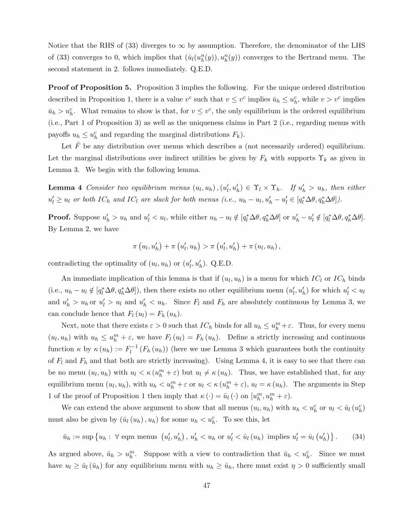
Notice that the RHS of (33) diverges to ∞ by assumption. Therefore, the denominator of the LHS

of (33) converges to 0, which implies that (ul(unh(y)), unh(y)) converges to the Bertrand menu. The

second statement in 2. follows immediately. Q.E.D.

Proof of Proposition 5. Proposition 3 implies the following. For the unique ordered distribution

described in Proposition 1, there is a value vc such that v ≤ vc implies uh ≤ uch, while v > vc implies

uh > uch. What remains to show is that, for v ≤ vc, the only equilibrium is the ordered equilibrium

(i.e., Part 1 of Proposition 3) as well as the uniqueness claims in Part 2 (i.e., regarding menus with

payoffs uh ≤ uch and regarding the marginal distributions Fk).

Let F be any distribution over menus which describes a (not necessarily ordered) equilibrium.

Let the marginal distributions over indirect utilities be given by Fk with supports Υk as given in

Lemma 3. We begin with the following lemma.

Lemma 4 Consider two equilibrium menus (ul, uh) , (ul, uh) ∈ Υl × Υh. If uh > uh, then either

ul ≥ ul or both ICh and ICl are slack for both menus (i.e., uh − ul, uh − ul ∈ [q∗l ∆θ, q∗h∆θ]).

Proof. Suppose uh > uh and ul < ul, while either uh − ul /∈ [q∗l ∆θ, q∗h∆θ] or uh − ul /∈ [q∗l ∆θ, q∗h∆θ].

By Lemma 2, we have

πul, u

h

+ π

ul, uh

> π

ul, u

h

+ π (ul, uh) ,

contradicting the optimality of (ul, uh) or (ul, uh). Q.E.D.

An immediate implication of this lemma is that if (ul, uh) is a menu for which ICl or ICh binds

(i.e., uh − ul /∈ [q∗l ∆θ, q∗h∆θ]), then there exists no other equilibrium menu (ul, uh) for which ul < ul

and uh > uh or ul > ul and uh < uh. Since Fl and Fh are absolutely continuous by Lemma 3, we

can conclude hence that Fl (ul) = Fh (uh).

Next, note that there exists ε > 0 such that ICh binds for all uh ≤ umh +ε. Thus, for every menu

(ul, uh) with uh ≤ umh + ε, we have Fl (ul) = Fh (uh). Define a strictly increasing and continuous

function κ by κ (uh) := F−1l (Fh (uh)) (here we use Lemma 3 which guarantees both the continuity

of Fl and Fh and that both are strictly increasing). Using Lemma 4, it is easy to see that there can

be no menu (ul, uh) with ul < κ (umh + ε) but ul = κ (uh). Thus, we have established that, for any

equilibrium menu (ul, uh), with uh < umh + ε or ul < κ (umh + ε), ul = κ (uh). The arguments in Step

1 of the proof of Proposition 1 then imply that κ (·) = ul (·) on [umh , umh + ε).

We can extend the above argument to show that all menus (ul, uh) with uh < uch or ul < ul (uch)

must also be given by (ul (uh) , uh) for some uh < uch. To see this, let

uh := supuh : ∀ eqm menus

ul, u

h

, uh < uh or ul < ul (uh) implies ul = ul

uh

. (34)

As argued above, uh > umh . Suppose with a view to contradiction that uh < uch. Since we must

have ul ≥ ul (uh) for any equilibrium menu with uh ≥ uh, there must exist η > 0 sufficiently small

47

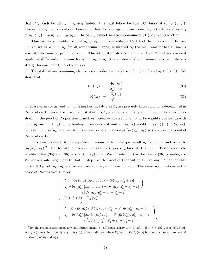
that ICh binds for all uh ≤ uh + η (indeed, this must follow because ICh binds at (ul (uh) , uh)).

The same arguments as above then imply that, for any equilibrium menu (ul, uh) with uh < uh + η

or ul < ul (uh + η), ul = ul (uh). Hence, uh cannot be the supremum in (34), our contradiction.

Thus, we have established that uh ≥ uch. This establishes Part 1 of the proposition: In case

v ≤ vc, we have uh ≤ uch for all equilibrium menus, as implied by the requirement that all menus

generate the same expected profits. This also establishes our claim in Part 2 that non-ordered

equilibria differ only in menus for which uh > uch (the existence of such non-ordered equilibria is

straightforward and left to the reader).

To establish our remaining claims, we consider menus for which uh ≥ uch and ul ≥ ul (uch). We

show that

Φh (uh) =

Φh (uh)

S∗h − uh

(35)

Φl (ul) =

Φl (ul)

S∗l − ul

(36)

for these values of uh and ul. This implies that Φl and Φh are precisely those functions determined in

Proposition 1; hence, the marginal distributions Fk are identical in any equilibrium. As a result, as

shown in the proof of Proposition 1, neither incentive constraint can bind for equilibrium menus with

uh ≥ uch and ul ≥ ul (uch) (a binding incentive constraint at (ul, uh) would imply Fl (ul) = Fh (uh),

but then ul = ul (uh) and neither incentive constraint binds at (ul (uh) , uh) as shown in the proof of

Proposition 1).

It is easy to see that the equilibrium menu with high-type payoff uch is unique and equal to

(ul (uch) , uch).

29 Neither of the incentive constraints ICl or ICh bind at this menu. This allows us to

establish that (35) and (36) hold at (ul (uch) , uch). We consider (35) as the case of (36) is analogous.

We use a similar argument to that in Step 1 of the proof of Proposition 1. For any ε ∈ R such that

uch + ε ∈ Υh, let (ul,ε, uch + ε) be a corresponding equilibrium menu. The same arguments as in the

proof of Proposition 1 imply

Φl (ul,ε) [Sl(ul,ε, uch)− Sl(ul,ε, uch + ε)]

+Φh (uch) [Sh(ul,ε, uch)− Sh(ul,ε, uch + ε) + ε]

εSh(ul,ε, uch + ε)− uch − ε

≤Φh (uch + ε)− Φh (uch)

ε

≤

Φl (ul (uch)) [Sl(ul (uch) , u

ch)− Sl(ul (uch) , u

ch + ε)]

+Φh (uch) [Sh(ul (uch) , uch)− Sh(ul (uch) , u

ch + ε) + ε]

εSh(ul

uch

, uch + ε)− uch − ε

.

29By the previous argument, any equilibrium menu (ul, uch) must satisfy ul ≥ ul (u

ch). If ul > ul (u

ch), then ICh binds

at (ul, uch) implying that Fl (ul) = Fh (uc

h), a contradiction (since Fh (uch) = Fl (ul (u

ch)) by the previous argument and

continuity of Fl and Fh).

48

We then use that30

limε→0

Sl(ul,ε, uch)− Sl(ul,ε, uch + ε)

ε= lim

ε→0

Sl(ul (uch) , uch)− Sl(ul (uch) , u

ch + ε)

ε= 0

and

Sh(ul,ε, uch)− Sh(ul,ε, u

ch + ε) = Sh(ul (u

ch) , u

ch)− Sh(ul (u

ch) , u

ch + ε) = 0

to conclude that

Φh (u

ch) =

Φh (uch)

S∗h − uch

.

Next, observe that there exists η > 0 such that incentive constraints are slack for any equilibrium

menu with uh ∈ [uch, uch + η]. This is obtained from (i) the above observation that if (ul, uh) is a

menu for which an incentive constraint ICk binds, then Fl (ul) = Fh (uh), and (ii) uch−ul (uch) = q∗l ∆θ

together with Φh (u

ch) < Φ

l (ul (uch)) (equivalently, F

h (u

ch) < F

l (ul (uch))).

As with the derivatives Φh (u

ch) and Φ

l (ul (uch)), one obtains (35) and (36) on [uch, u

ch + η]. We

then use again that Fl (ul) = Fh (uh) for any menu (ul, uh) for which an incentive constraint binds

to obtain that the constraints must be slack for any equilibrium menu with uh ≥ uch. To see this,

let

u#h = supuh : ICl and ICh are slack for all eqm. menus

ul, u

h

with uh ∈ [uch, uh]

.

The above property, together with continuity of Fl and Fh, implies that, if u#h < uh, then u#h −u#l /∈(∆θq∗l ,∆θq∗h) for u

#l satisfying Fl

u#l

= Fh

u#h

. However, Fl and Fh must agree with functions

derived in Proposition 1 on, respectively,uml , ul

u#h

and

umh , u#h

. Hence u#l = ul

u#h

. This

contradicts our finding in the proof of Proposition 1 that u#h − ulu#h

∈ (∆θq∗l ,∆θq∗h). Q.E.D.

7 Appendix B: Competition and Market Coverage with a Contin-

uum of Types

The aim of this section is to extend the binary-types model developed in the paper to a continuum-

type setting, thus confirming that our main insights are robust to this more general environment.

For tractability, we let consumer valuations be uniformly distributed in the unit interval [0, 1], and

assume that firms costs are quadratic: ϕ(q) = 12 · q

2. The reason for these assumptions is the follow-

ing: Characterizing an ordered equilibrium with a continuum of types requires solving a nonlinear

partial differential equation with nonstandard boundary conditions (as will be described below). For

arbitrary distributions of valuations and cost functions, this equation does not admit a closed-form

30This follows after noticing that, for any ν > 0, there exists ι > 0 such that, for all |ε| < ι, uch−ul,ε ∈ (∆θq∗l −ν,∆θq∗h].

This follows after noticing that either both incentive constraints are slack at (ul,ε, uch + ε), or one of ICl and ICh bind,

in which case ul,ε = F−1l (Fh (uc

h + ε)), which tends to ul (uch) as ε → 0.

49

solution, and the (few) existence results available in the literature on partial differential equations

do not apply. While we believe that our results extend to environments other than the uniform-

quadratic, computing equilibria in such environments requires numerical techniques which are out

of the scope of this work.31

The analysis proceeds analogously to that of Section 3. Firms post price-quality menus M ≡((q(θ), x(θ)) : θ ∈ [0, 1]) , where q(θ) is the quality, and x(θ) is the price of the contract designed for

type θ. We let u(θ) ≡ θ · q(θ) − x(θ) be the indirect utility of type θ. By standard arguments, a

menu M is incentive compatible (IC) if and only if the indirect utility schedule u(·) is absolutely

continuous (with derivative u(θ) = q(θ) almost everywhere), and convex. The set of all menus Mthat are incentive compatible and individually rational (i.e., u(θ) ≥ 0 for all θ ∈ [0, 1]) is denoted by

I. For convenience, and in light of incentive compatibility, we write M = u(·) to describe the menu

M ≡ ((q(θ), x(θ)) : θ ∈ [0, 1]) , where q(θ) = u(θ) and x(θ) = θ · u(θ)− u(θ) for almost every θ.

As in the model with binary types, we model the heterogeneity of information possessed by

consumers by means of sales functions satisfying Assumption 1. For a given cross-section distribution

over menus F (with support S ⊆ I), we denote by F (u; θ) the marginal distribution over indirect

utilities for each type θ (with support Υ(θ)). We can therefore write a firm’s profit-maximization

problem as that of choosing an indirect utility schedule u(·) to maximize the functional

π[u] ≡ˆ 1

0Λ (F (u(θ); θ)|v) ·

θ · u(θ)− u(θ)− 1

2·u(θ)

2dθ. (37)

The expression above computes the total profits of a menu u(·) by integrating the product of the

sales volume, Λ (F (u(θ); θ)|v), with the profits per sale, x(θ)− 12 · q(θ)2, over all types θ ∈ [0, 1].

Analogously to the binary type model, we focus on ordered equilibrium, as formally defined

below.

Definition 3 [Ordered Equilibrium] An ordered equilibrium is a distribution over menus F (with

marginal distribution over type-θ indirect utilities F (·; θ)) such that

1. M = u(·) ∈ S ⊆ I implies that M = u(·) maximizes (37),

2. if u(·), u(·) ∈ S, and u(θ) > u(θ) for some θ ∈ [0, 1], then u(θ) ≥ u(θ) for all θ ∈ [0, 1], with

strict inequality whenever u(θ) > 0.

The first condition in the definition above is the usual profit-maximization requirement. The

second condition captures the “ordered” feature of our equilibrium: If a menu is “more generous” to

one type of consumer, then it is more generous to all consumer types that are served by that menu.

As in the case with binary types, it is convenient to describe the support S by indexing each

schedule u(·) ∈ S by the indirect utility received by the highest type θ = 1. Accordingly, we denote

31Below, we derive general necessary conditions of equilibria that might be amenable to numerical analysis.

50

by V (θ, u) the indirect utility received by type θ in the menu where the highest type θ = 1 obtains

utility u. For a given ordered equilibrium, we refer to the bivariate function V (·, ·) as its support

schedule. Note that V (θ, u) is strictly increasing in u at every type θ that is not excluded (i.e,

V (θ, u) > 0).

We further restrict attention to equilibria exhibiting the following “smoothness” properties.

We say that an ordered equilibrium is smooth if at every pair (θ, u) such that V (θ, u) > 0 the

following conditions hold: (i) the support schedule V (θ, u) is twice continuously differentiable in

θ, and continuously differentiable in u , (ii) the distribution of type-θ indirect utilities, F (·; θ), isabsolutely continuous with density f(·; θ), and (iii) the mapping F (u; θ) is continuously differentiable

in θ for each u.

7.1 Equilibrium Characterization

The next proposition describes a smooth ordered equilibrium.

Proposition 6 [Equilibrium Characterization - Continuum of Types] There exists a smooth

ordered equilibrium. In this equilibrium, the support of indirect utilities offered by firms is described

by the support schedule

V (θ, u) = max

1

4 · u · θ2 +1− 1

2 · u

· θ + u+

1

4 · u − 1, 0

, (38)

with domain on [0, 1]× [14 ,12 ].

The equilibrium distribution over menus for the highest type solves

Λ (F (u; 1)|v)Λ (0|v) =

148´ 1

0

θ · V1(θ, u)− V (θ, u)− 1

2 · [V1(θ, u)]2dθ

, (39)

where the supremum point of Υ(1), denoted ¯u, is determined by F (¯u; 1) = 1.

Equilibrium Construction. The equilibrium construction under a continuum of types closely

mirrors that of the binary type model from the previous section. First, the ordered nature of

equilibrium, together with the ranking property of kernels, implies that

Λ (F (u; 1)|v) = Λ (F (V (θ, u); θ)|v) (40)

at every pair (θ, u) such that V (θ, u) > 0. Differentiating the expression above with respect to u

leads to the continuous analogue of equation (15):

V2(θ, u) =Λ1 (F (u; 1)|v) · f(u; 1)

Λ (F (u; 1)|v) ·Λ1 (F (V (θ, u); θ)|v) · f (V (θ, u); θ))

Λ (F (V (θ, u); θ)|v)

−1

, (41)

51

which states that the partial derivative of the support schedule with respect to u at (θ, u) equals the

ratio between the semi-elasticities of sales with respect to indirect utilities between the highest type

and type θ.

Second, for a smooth equilibrium, the optimality of equilibrium menus implies that the following

Euler equation must hold at any (θ, u) where V (θ, u) > 0:

Λ1 (F (V (θ, u); θ)|v) · f(V (θ, u); θ) ·θ · V1(θ, u)− V (θ, u)− 1

2(V1(θ, u))

2

sales gains

= Λ (F (V (θ, u); θ)|v) profit losses

+ Λ (F (V (θ, u); θ)|v) · d

dθθ − V1(θ, u)

efficiency effect

. (42)

Analogously to the first-order conditions (7) and (8), the Euler equation above identifies the

three effects that determine the firms’ optimal choice of menus. The first term captures the effect

of generosity on sales, while the second effect accounts for the effect of generosity on profits per

sale. More interestingly, the third term captures the effect of increasing the indirect utility of type

θ on the quality distortions of its “adjacent” types (as implied by incentive constraints). Similarly

to the binary type model, the optimality condition alone is not enough to sign the efficiency effect:

While increasing the indirect utility of type θ allows the firm to decrease quality distortions to its

“lower neighbors”, it also tightens the IC constraints of its “upper neighbors” (which leads to higher

distortions).

Combining the ranking condition (41) with the optimality condition (42) leads to the follow-

ing partial differential equation, that the support schedule has to satisfy in any smooth ordered

equilibrium:

V2(θ, u) =2− V11(1, u)

2− V11(θ, u)·θ · V1(θ, u)− V (θ, u)− 1

2 · (V1(θ, u))2

12 − u

. (43)

The partial differential equation above is the analogue of the ordinary differential equation (12) from

Proposition 1. Guided by the binary type model, we posit that the support schedule has to satisfy

the following boundary conditions:

V

θ,

1

4

= max

θ2 − θ +

1

4, 0

, V

θ,

1

2

=

θ2

2, V1(1, u) = 1, and V (1, u) = u. (44)

The first boundary condition in (44) states that the Mussa-Rosen menu is the “lowest” menu in

the support S (in the sense that it provides the lowest indirect utility to every type). Intuitively,

the firm that offers the least generous menu is preferred to any other firm known to the consumer.

Therefore, this firm must offer the monopoly menu. The second boundary condition guarantees that

equilibrium menus approach the Bertrand (or efficient) menu as firms relinquish the total surplus

to consumers. The third boundary condition requires that the highest type is offered the efficient

52

Figure 3: The quality schedules associated with u = 0.25, 0.3, 0.35, 0.4, 0.45, 0.5, from the bottom

to the top curves, respectively. The bottom curve is the Mussa-Rosen quality schedule, while the top

curve is the Bertrand quality schedule. The schedules offered in equilibrium are those with u ≤ ¯u.

quality in all menus in S. The last boundary condition requires that the solution to (43) be consistent

with the definition of the support schedule V (θ, u).

The support schedule V (θ, u) in equation (38) solves the partial differential equation (43) subject

to the boundary conditions in (44). In the proof of Proposition 6, contained in the Appendix, we

formalize the equilibrium construction sketched above. Most importantly, we establish that the Euler

equation (42) is a necessary and sufficient condition that any menu that maximizes (37) has to satisfy,

and rule out deviations to menus that offer out-of-equilibrium contracts to any type.

Finally, similarly to Proposition 1, the indifference condition (42) guarantees that all menus

offered in equilibrium lead to the same total profits as the Mussa-Rosen menu. As before, the

matching technology, captured by the kernel Λ (y|v), determines the upper limit in the support of

indirect utilities to the highest consumer type, ¯u, as well as its cumulative distribution function,

F (u; 1). By virtue of the ordered nature of the equilibrium, the distribution over indirect utilities of

any type θ ∈ [0, 1) can be recovered from equation (40).

7.2 Equilibrium Properties

Let us start our discussion of equilibrium properties with the relationship between generosity and

distortions. To do so, let us consider the collection of quality schedules

q(θ, u) ≡ V1(θ, u) = max

1

2 · u · θ +1− 1

2 · u

, 0

, (45)

53

indexed by the indirect utility offered to the highest type. First, we see that whenever q(θ, u) > 0

we have that∂q(θ, u)

∂u=

1− θ

2u2> 0.

Therefore, as in the binary type model, distortions decrease for all types as firms offer more generous

menus. Figure 3 above depicts some quality schedules offered in equilibrium.

We now consider the effects of competition on market coverage. From (45), the range of types

served by a menu with highest-type utility u is the interval [α(u), 1], where

α(u) = 1− 2u. (46)

It follows from (46) that α(u) is decreasing in u. Therefore, firms segment themselves according

to the range of consumer types served by their menus, which we call inclusiveness. As such, more

generous firms, as captured by u, are also more inclusive, in the sense that they serve a larger range of

types. At one extreme lies the Mussa-Rosen menu, which is the least generous and the least inclusive

equilibrium menu. At the other extreme lies the menu associated with highest-type indirect utility

¯u, which is the most generous and most inclusive menu offered in equilibrium. This is illustrated in

Figure 3 above.

Finally, and analogously to the binary-type model, firms that offer more generous menus make

more sales to consumers with low willingness to pay. Formally, for each θ ∈ (0, 1), the share of

profits obtained from consumers with type θ ∈ [0, θ] is increasing in u. We collect these findings in

Proposition 7.

Proposition 7 [Equilibrium Properties] The following properties hold in the ordered equilibrium

of Proposition 6.

1. Efficiency: Menus for which consumers earn higher payoffs are more efficient, i.e., q(θ, u) is

increasing in u, strictly whenever θ < 1 and q(θ, u) > 0.

2. Inclusiveness: Firms that offer more generous contracts serve a larger set of consumers, i.e.,

the range [α(u), 1] of types served expands as u increases.

3. Profits: Firms that offer more generous menus derive a greater share of profits from con-

sumers with low willingness to pay, i.e., relative to total profits, the ratio of profits derived

from consumers with types in any interval of the form [0, θ], where θ < 1, is increasing in u.

7.3 Comparative Statics

The continuous-type model of this section enables us to study how the range of types served in

equilibrium, [α(¯u), 1], which we call market coverage, is affected by competition.

54

The next proposition shows that the equilibrium market coverage monotonically approaches

its competitive level as the mass of firms increases. At one extreme, as v → 0, the equilibrium

market coverage approaches its monopolistic level, where only consumers with willingness to pay in

the interval12 , 1

are served. At the other extreme, as v → ∞, the equilibrium market coverage

approaches its efficient level, i.e., full market coverage.

Proposition 8 [Competition and Market Coverage: Comparative Statics] Consider the

smooth ordered equilibrium of Proposition 6, and assume that condition VM holds. Denote by F (·; θ)and F (·; θ) the equilibrium distributions over indirect utilities of type θ when the mass of firms is v

and v, respectively.

1. If v > v, then F (·; θ) first-order stochastically dominates F (·; θ) for all θ ∈ [0, 1]. In particular,

the equilibrium market coverage, [α(¯u), 1], expands as v increases.

2. If limv→0R(1|v) = 1, then, as the mass of firms converges to zero, v → 0, the equilibrium

distribution over menus converges to a degenerate distribution centered at the monopolistic

(Mussa-Rosen) menu. In particular, the equilibrium market coverage monotonically converges

to its monopoly level.

3. If limv→∞R(y|v) = ∞ for all y ∈ (0, 1], then, as the mass of firms grows large, v → ∞,

the distribution over menus converges to a degenerate distribution centered at the competitive

(Bertrand) menu. In particular, the equilibrium market coverage monotonically approaches

[0, 1], i.e., full market coverage.

Similarly to Section 3, the results above can be recast in terms of the levels of frictions of the

matching technology, as discussed in Remarks 4 and 5.

Proofs of results for continuum-types model

7.4 Outline

The goal of this section is to prove Proposition 6. We start in Section 5.5 deriving necessary conditions

for a smooth ordered equilibrium for a general type distribution and cost function. As we will see,

these necessary conditions involve a solution to a partial differential equation which relates the quality

schedule of a certain menu to its generosity. In Section 5.6 we specialize to the uniform quadratic

case. We start by postulating a closed-form solution to this partial differential equation, and we

check it is a solution in Section 5.6.1. Given this solution, we are able to propose an equilibrium

allocation in Section 5.6.2. The rest of the appendix is then devoted to verifying that we have an

55

equilibrium. In Section 5.6.3 we verify that all menus in the support of the proposed allocation

yield the same profit. Next, in Section 5.6.4 we invoke a calculus of variations existence theorem to

show that the firms’ problem has a solution. Finally, in Section ?? we show that the only menus

satisfying calculus of variations necessary conditions for an optimum are those found in the support

of the putative equilibrium menus. This shows that all equilibrium menus maximize firm profits, as

required.

7.5 General Necessary Conditions

Here we will derive the analogue for a continuum of types of the support function obtained in the

case of a binary type space. As described in the main text, the firms’ problem is to choose an

indirect utility schedule u(θ) to maximize

ˆ θ

θΛ (F (u(θ); θ) |v) · (θ · u(θ)− ϕ(u(θ))− u(θ)) · h(θ)dθ, (47)

where Λ is the kernel of the matching technology, ϕ(q) is the cost of producing a good of quality

q, and h(θ) is the density of type θ (with support [θ, θ]). In order to ease the notation below we

suppress the dependence of Λ on v, writing Λ (F (V (θ, u); θ)) for Λ (F (V (θ, u); θ) |v) .We posit that in equilibrium each firm is indifferent between choosing any schedule in some

support S. Each of the schedules u(θ) in S are strictly increasing and weakly convex in θ (that is,

there is an implementable direct-revelation mechanism delivering an indirect utility u(θ)).

We can conveniently describe the support S by indexing each schedule by the indirect utility

received by type θ. Denote by V (θ, u) the indirect utility received by type θ when type θ obtains

utility u. Note that V (θ, u) = u. The set of indirect utility schedules is then

S =V (θ, u) : u ∈ [um, S∗]

,

where um is the Mussa-Rosen indirect utility of type θ, and S∗ is the Bertrand indirect utility of

type θ: S∗ ≡ maxqθ · q − ϕ(q)

. Given that we wish to characterize a smooth equilibrium, we look

for a support schedule V (θ, u) which is twice continuously differentiable at every point such that

V (θ, u) > 0.

It is a property of the ordered equilibrium that for any two types θ, θ ∈ [θ, θ] such that

V (θ, u), V (θ, u) > 0

Λ (F (V (θ, u); θ)) = ΛFV (θ, u); θ

. (48)

It is an implication of (48) thatd

dθΛ (F (V (θ, u); θ)) = 0. (49)

That V (θ, u) = u implies

Λ (F (V (θ, u); θ)) = ΛFu; θ

.

56

Differentiating with respect to u leads to

Λ(F (V (θ, u); θ)) · f (V (θ, u); θ) · V2(θ, u) = Λ(F (u; θ)) · fV (θ, u); θ

. (50)

Optimality implies that every menu V (θ, u) ∈ S has to satisfy the following Euler equation at

any θ where V (θ, u) > 0:

Λ(F (V (θ, u); θ)) · f (V (θ, u); θ) · (θ · V1(θ, u)− ϕ (V1(θ, u))− V (θ, u)) · h(θ)−Λ(F (V (θ, u); θ)) · h(θ)

=d

dθ

Λ(F (V (θ, u); θ)) ·

θ − ϕ(V1(θ, u))

· h(θ)

. (51)

Because of (49), it follows that

d

dθ

Λ(F (V (θ, u); θ)) ·

θ − ϕ(V1(θ, u))

· h(θ)

= Λ(F (V (θ, u); θ)) · d

dθ

θ − ϕ(V1(θ, u))

· h(θ)

. (52)

Plugging (52) into (51) and manipulating leads to:

Λ(F (V (θ, u); θ))

Λ(F (V (θ, u); θ))· f (V (θ, u); θ) =

h(θ) + ddθ (θ − ϕ(V1(θ, u))) · h(θ)

(θ · V1(θ, u)− ϕ (V1(θ, u))− V (θ, u)) · h(θ) . (53)

Let us choose θ = θ in (53) to obtain that:

Λ(Fu; θ

)

Λ(Fu; θ

)· f

u; θ

=

h(θ) + ddθ (θ − ϕ(V1(θ, u))) · h(θ)θ=θ

θ · V1(θ, u)− ϕV1(θ, u)

− u

· h(θ)

. (54)

Note that

Λ(F (V (θ, u); θ))

Λ(F (V (θ, u); θ))· f (V (θ, u); θ)

−1

·Λ(F

u; θ

)

Λ(Fu; θ

)· f

V (θ, u); θ

= V2(θ, u), (55)

where the equality follows from (50).

Dividing (54) by (53), and using the relation (55), we then obtain that

V2(θ, u) =(θ · V1(θ, u)− ϕ (V1(θ, u))− V (θ, u)) · h(θ)θ · V1(θ, u)− ϕ

V1(θ, u)

− V (θ, u)

· h(θ)

·h(θ) + d

dθ (V1(θ, u)− ϕ(V1(θ, u))) · h(θ)θ=θ

h(θ) + ddθ (V1(θ, u)− ϕ(V1(θ, u))) · h(θ)

.

We posit that in the ordered equilibrium the highest type θ is always assigned the efficient quality

level. The PDE is then

V2(θ, u) =(θ · V1(θ, u)− ϕ (V1(θ, u))− V (θ, u)) · h(θ)

S∗ − u· h(θ)

·h(θ) + d

dθ (V1(θ, u)− ϕ(V1(θ, u))) · h(θ)θ=θ

h(θ) + ddθ (V1(θ, u)− ϕ(V1(θ, u))) · h(θ)

.

(56)

57

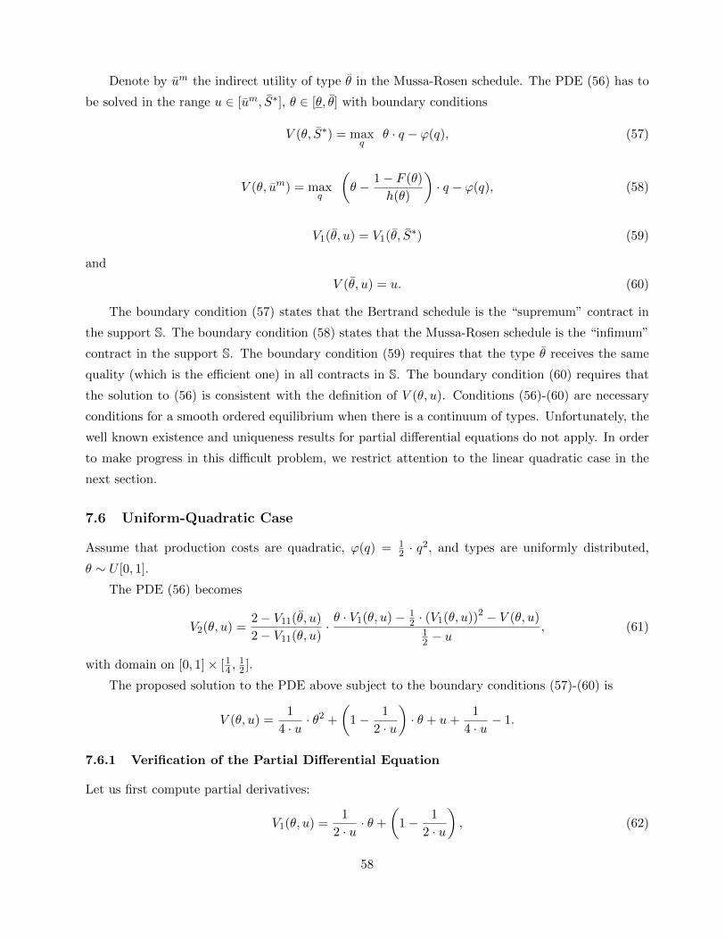
Denote by um the indirect utility of type θ in the Mussa-Rosen schedule. The PDE (56) has to

be solved in the range u ∈ [um, S∗], θ ∈ [θ, θ] with boundary conditions

V (θ, S∗) = maxq

θ · q − ϕ(q), (57)

V (θ, um) = maxq

θ − 1− F (θ)

h(θ)

· q − ϕ(q), (58)

V1(θ, u) = V1(θ, S∗) (59)

and

V (θ, u) = u. (60)

The boundary condition (57) states that the Bertrand schedule is the “supremum” contract in

the support S. The boundary condition (58) states that the Mussa-Rosen schedule is the “infimum”

contract in the support S. The boundary condition (59) requires that the type θ receives the same

quality (which is the efficient one) in all contracts in S. The boundary condition (60) requires that

the solution to (56) is consistent with the definition of V (θ, u). Conditions (56)-(60) are necessary

conditions for a smooth ordered equilibrium when there is a continuum of types. Unfortunately, the

well known existence and uniqueness results for partial differential equations do not apply. In order

to make progress in this difficult problem, we restrict attention to the linear quadratic case in the

next section.

7.6 Uniform-Quadratic Case

Assume that production costs are quadratic, ϕ(q) = 12 · q2, and types are uniformly distributed,

θ ∼ U [0, 1].

The PDE (56) becomes

V2(θ, u) =2− V11(θ, u)

2− V11(θ, u)·θ · V1(θ, u)− 1

2 · (V1(θ, u))2 − V (θ, u)

12 − u

, (61)

with domain on [0, 1]× [14 ,12 ].

The proposed solution to the PDE above subject to the boundary conditions (57)-(60) is

V (θ, u) =1

4 · u · θ2 +1− 1

2 · u

· θ + u+

1

4 · u − 1.

7.6.1 Verification of the Partial Differential Equation

Let us first compute partial derivatives:

V1(θ, u) =1

2 · u · θ +1− 1

2 · u

, (62)

58

and

V2(θ, u) = − 1

4 · u2 · θ2 + 1

2 · u2 · θ + 1− 1

4 · u2 .

Let us first verify the boundary conditions. To verify (57), note that S∗ = 12 . Therefore,

V (θ, S∗) = V

θ,

1

2

=

1

2· θ2 = max

qθ · q − 1

2· q2.

To verify (58), note that um = 14 . Therefore,

V (θ, um) = V

θ,

1

4

= θ2 − θ +

1

4= max

q(2 · θ − 1) · q − 1

2· q2.

To verify (59), note that

V1(1, u) =1

2 · u +

1− 1

2 · u

= 1.

To verify (60), note that

V (1, u) =1

4 · u + 1− 1

2 · u + u+1

4 · u − 1 = u.

To verify that (61) is satisfied, note that

θ · V1(θ, u)−1

2· (V1(θ, u))

2 − V (θ, u)

= θ ·

1

2 · u · θ +1− 1

2 · u

− 1

2·

1

2 · u · θ +1− 1

2 · u

2

− 1

4 · u · θ2 −1− 1

2 · u

· θ − u− 1

4 · u + 1,

which, after some algebra, can be shown to be equal to1

2− u

·− 1

4 · u2 · θ2 + 1

2 · u2 · θ + 1− 1

4 · u2

=

1

2− u

· V2(θ, u).

Because V11(θ, u) = V11(θ, u), it follows that (61) holds.

7.6.2 Ordered Equilibrium

Next, we use the family of curves (V (θ, u))θ∈[0,1] for u ∈ [14 ,12 ] to propose the equilibrium distribu-

tion over menus F . From (54) and the knowledge of V we obtain a unique ¯u ∈14 ,

12

such that´ ¯u

14f(u; 1)du = 1. Therefore, in the proposed equilibrium, the firms offer menus (V (θ, u))θ∈[0,1] for

u ∈ [14 , ¯u] such that a menu less generous than (V (θ, u))θ∈[0,1] is offered with probability F (u; 1).

The rest of this appendix verifies that no firm has a profitable deviation. We start verifying that all

menus in S yield the same profit.

59

7.6.3 Checking Indifference

Here we verify that all menus (V (θ, u))θ∈[0,1] for u ∈ [14 , ¯u] lead to the same profit. We have:

Π(u) ≡ˆ θ

α(u)Λ(F [V (θ, u); θ]) ·

θ · V1(θ, u)−

1

2· (V1(θ, u))

2 − V (θ, u)

dθ,

where α(u) solves

V1(α(u), u) = 0.

It is easy to verify that V (α(u), u) = 0.

To simplify notation, let

L (V (θ, u), V1(θ, u), θ) ≡ Λ(F [V (θ, u); θ]) ·θ · V1(θ, u)−

1

2· (V1(θ, u))

2 − V (θ, u)

.

Then

Π(u) ≡ˆ θ

α(u)L1 (V (θ, u), V1(θ, u), θ) · V2(θ, u) dθ

+

ˆ θ

α(u)L2 (V (θ, u), V1(θ, u), θ) · V12(θ, u) dθ

−L (V (α(u), u), V1(α(u), u),α(u)) · α(u). (63)

Integration by parts delivers that

ˆ θ

α(u)L2 (V (θ, u), V1(θ, u), θ) · V12(θ, u) dθ

= L2 (V (θ, u), V1(θ, u), θ) · V2(θ, u)|θα(u)

−ˆ θ

α(u)V2(θ, u) ·

d

dθ[L2 (V (θ, u), V1(θ, u), θ)]

dθ.

Plugging the above into (63) and using the fact V (θ, u) solves the Euler equation for

every (θ, u) with θ > α(u) leads to

Π(u) = L2 (V (θ, u), V1(θ, u), θ) · V2(θ, u)|θα(u) − L (V (α(u), u), V1(α(u), u),α(u)) · α(u).

Note that

L2V (θ, u), V1(θ, u), θ

= Λ(F

V (θ, u); θ

) ·

θ − V1(θ, u)

= 0.

60

Recall that V (α(u), u) = 0. Total differentiation yields

V1(α(u), u) · α(u) + V2(α(u), u) = 0.

Because by construction V1(α(u), u) = 0, it follows that V2(α(u), u) = 0. This implies

that

L2 (V (θ, u), V1(θ, u), θ) · V2(θ, u)|θα(u) = 0.

Finally, because V (α(u), u) = 0 and V1(α(u), u) = 0,

L (V (α(u), u), V1(α(u), u),α(u)) = 0.

This establishes that Π(u) = 0 for all u ∈ [14 , ¯u], implying that all proposed menus yield the same

profit.

7.6.4 Existence of a Solution

We write Ψ(u, θ) for the sales function from offering a utility u to the type θ : Ψ(u, θ) ≡ Λ(F (u; θ)).

For every u ∈14 , ¯u

write (uu (θ)) for the curve (V (θ, u))θ∈[0,1] . We write AC[0, 1] for the space of

absolutely continuous functions from [0, 1] into R. Hence, we can write the firm’s problem as:

maxu∈AC[0,1]

ˆ 1

0Π(θ, u (θ) , u (θ))dθ, (64)

where

Π(θ, u, u) ≡ Ψ(u, θ)

θ · u− 1

2· (u)2 − u

.

We consider the relaxed problem in which u (θ) = q(θ) ∈ R and q(θ) need not be monotonic.

Lemma 5 invokes a calculus of variations existence theorem to show that (64) has a solution.

Lemma 5 The problem (64) has a solution.

Proof. Let A ≡ supu,θ Ψ(u, θ). It is straightforward to see that we may restrict attention to

allocations such thatθ · u− 1

2 · (u)2 − u≥ 0 for almost all θ. Therefore

Π(θ, u, u) ≤ A[u− 1

2· (u)2] = Au

1− 1

4· u

−A

4

· (u)2

≤ A−A

4

· (u)2 .

Hence, we may assume that Π is coercive of degree 2, that is, Π(θ, u, u) ≤ A−A4

· (u)2 for (almost)

every (θ, u, u). Furthermore, notice that Π(θ, u, u) is continuous in (θ, u, u) and it is concave in u. The

existence of an absolutely continuous solution follows from Theorem 16.2 in Clarke (2013). Q.E.D.

61

Conclusion

We will show that the solutions to (64) are the curves (uu (θ)) for u ∈14 , ¯u

. Our approach is to (i)

show that we must have u∗ (1) ∈14 , ¯u

for any optimal menu u∗, and (ii) show that, for each value

of u∗ (1) ∈14 , ¯u

, the necessary condition for the menu u∗ (θ) to be optimal in (64) admits a unique

solution, which is the menu given by uu∗(1) (θ). Thus, the only candidates for optima in (64) are

the curves (uu (θ)), u ∈14 , ¯u

, identified above.

We now outline the proof in more detail. In the proof, we will use Theorem 18.1 in Clarke (2013),

which provides necessary conditions for optimal solutions of calculus of variations problems. Hence,

we first check that the conditions for Theorem 18.1 hold. Next, we consider an optimal allocation

(u∗ (θ)) and divide the analysis into five exhaustive cases.

Case 1 deals with u∗ (1) ∈u 1

4(1) , u¯u(1)

. We show that the Euler equation (51) is necessary.

Moreover, this Euler equation leads to an ordinary differential equation which has a unique solution,

as desired.

Case 2 deals with the possibility that u∗ (1) > u¯u(1). We show that (51) then implies u∗ (θ) is

bounded above u¯u(θ) for all θ; hence (u∗ (θ)) cannot be optimal.

Case 3 deals with the possibility that u∗ (1) < u 14(1). We consider two cases. First, assume

that the curves (u∗ (θ)) andu 1

4(θ)

never intersect in

12 , 1

. In this case, the firm could profitably

deviate by offering the menuu 1

4(θ)

. Second, assume that the curves (u∗ (θ)) and

u 1

4(θ)

intersect

at some θ∗ ∈12 , 1

. In this case, our argument below implies that the firm could profitably deviate

by offering the curve (remember that we are considering a relaxed problem in which monotonicity

constraints are ignored):

u∗∗ (θ) :=

u 1

4(θ) if θ > θ∗

u∗ (θ) otherwise.

Hence we conclude that this case is not possible.

Case 4 deals with the case that u∗ (1) = u¯u(1). This case is complicated by the fact that

the function Ψ is not differentiable along the curve (u¯u(θ)) , since Ψ (u, θ) = Ψ (u, θ) whenever

min u, u ≥ u¯u(θ). Therefore, we have 0 = Ψ1 (u¯u(θ)+, θ) < Ψ1 (u¯u(θ)−, θ).32 The proof is thus

divided into two cases. First, it is assumed that there is θ ∈ (0, 1) such that u∗ (θ) > u¯u(θ). The

Euler equation (51) then implies that u∗ (θ) > u¯u(θ) for all θ < θ and that u∗ (θ) < 0 for sufficiently

small θ, which contradicts the optimality of (u∗ (θ)).

Thus we may assume that u∗ (θ) ≤ u¯u(θ) for every θ. We proceed as follows. First, we use

calculus of variations necessary conditions which do not require differentiability.33 Roughly, when

the function Ψ fails to be differentiable along the curve u∗(θ) we have a generalized Euler equation in

32For a function h : 2 → we write h1 (a−, b) for limx→a−h(x,b)−h(a,b)

x−a and h1 (a+, b) for limx→a+h(x,b)−h(a,b)

x−a .33We follow the analysis of Clarke (2013). Definitions are given in the proof of Proposition 6 below.

62

which a subgradient ξ (θ) ∈ ∂1Ψ (u∗(θ), θ) plays the role of the the derivative of Ψ (u∗(θ), θ) .34 In this

case, we show that the generalized Euler equation picks the left subgradient Ψ (u∗(θ), θ) with respect

to u for almost every point. Hence, the fact that Ψ is not differentiable along the curve (u∗(θ)) is

immaterial and the conclusion that (u∗ (θ)) = (u¯u(θ)) follows from the argument given in Case 1.

Heuristically, our argument proceeds as follows. Suppose we have an interval [θα, θβ ] in which the

Euler equation picks a subgradient ξ (θ) < Ψ1 (u∗(θ)−, θ) . Therefore, since Ψ is not differentiable

only along the curve (u¯u(θ)) it must be that (for θα sufficiently close to θβ):

u∗(θ) = u¯u(θ) ∀θ ∈ [θα, θβ ] . (65)

Recall that the curve (u¯u(θ)) is constructed by the Euler equation in which the subgradientΨ (u¯u(θ)−, θ)

is selected and that u∗ (θβ) = u¯u(θβ). Hence, since ξ (θ) < Ψ1 (u¯u(θ)−, θ) for every θ ∈ [θα, θβ ] the

curves (u¯u(θ)) and (u∗(θ)) drift apart for θ sufficiently close to θβ , which contradicts (65).35

Case 5 deals with the case that u∗ (1) = u 14(1). We show that the function Ψ is differentiable

alongu 1

4(θ) , θ

θ> 12

. Therefore, the difficulties which arose in Case 4 do not appear here and an

argument analogous to the one from Case 1 implies that (u∗ (θ)) =u 1

4(θ)

.

Proof of Proposition 6. Write (u∗ (θ)) for an optimal menu. We will show that for every u ∈14 , ¯u

the menu (uu (θ)) is optimal. Our proof will use the necessary conditions from Theorem 18.1 in

Clarke (2013). In order to use this Theorem, we must check that our primitives satisfy the following

Lipschitz condition.

Conditions for application of Theorem 18.1 in Clarke (2013). Let K > 0 be such that

|Ψ(uβ (θ) , θ)−Ψ(uγ (θ) , θ)| ≤ K |uβ (θ)− uγ (θ)| for all curves (uβ (θ)) , (uγ (θ)) ∈ AC[0, 1] and all

θ. Since maxq,θθ · q − 1

2 · q2 ≤ 1

2 we have, for all (uβ (θ)) , (uγ (θ)) ∈ AC[0, 1], all θ,

|Π(θ, uβ (θ) , uβ (θ))−Π(θ, uγ (θ) , uγ (θ))|

=

Ψ(uβ (θ) , θ)

θ · uβ (θ)−

1

2· (uβ (θ))2 − uβ (θ)

−Ψ(uγ (θ) , θ)

θ · uγ (θ)−

1

2· (uγ (θ))2 − uγ (θ)

≤ K |uβ (θ)− uγ (θ)|+KA |uβ (θ)− uγ (θ)| .

Hence the Lipschitz condition (LH) in page 348 of Clarke (2013) is satisfied, allowing application of

Theorem 18.1 in Clarke (2013).

We have five cases.

Case 1: u∗ (1) ∈u 1

4(1) , u¯u(1)

.

34For a function h : 2 → , we write ∂1h (a, b) for all subgradients of the function x → h(x, b) at h (a, b) .35The proof would follow essentially the steps that we just explained if we could assume that the Euler equation

picks a subgradient ξ (θ) ∈ ∂1Ψ (u ¯u(θ), θ)− ε in an interval [θα, θβ ] . However, assuming that such property holds in an

entire interval may be with loss of generality, which makes the formal analysis below a little more complicated.

63

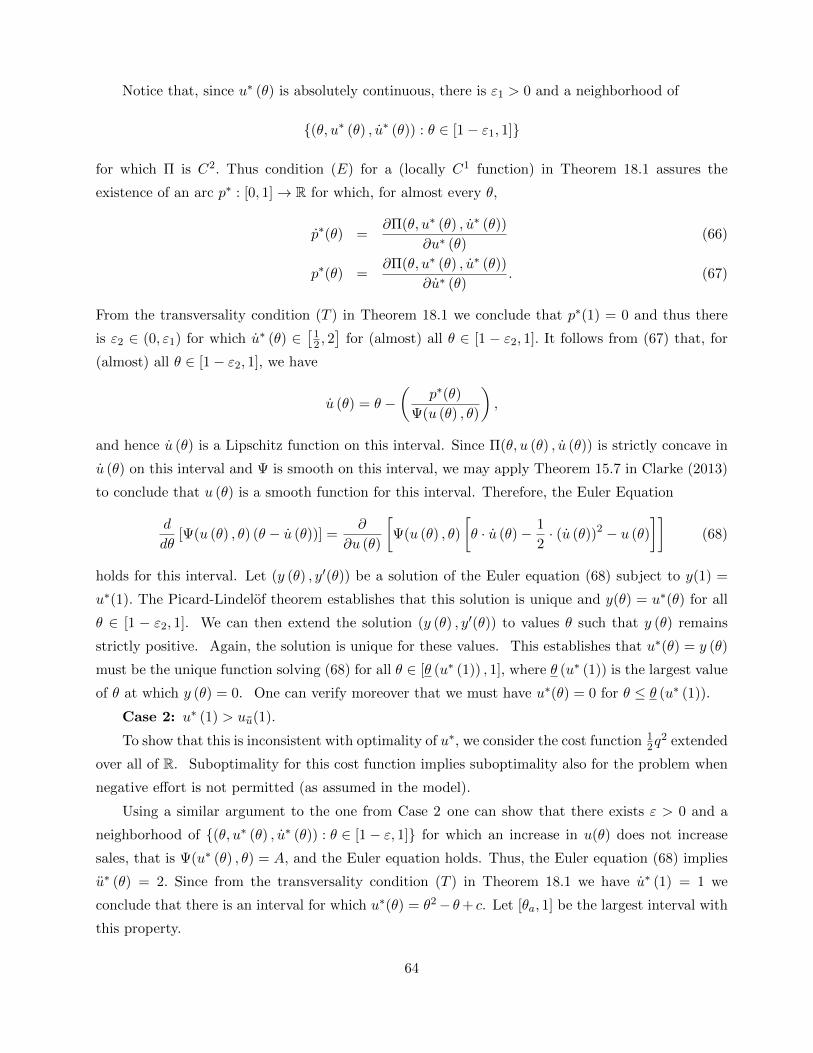
Notice that, since u∗ (θ) is absolutely continuous, there is ε1 > 0 and a neighborhood of

(θ, u∗ (θ) , u∗ (θ)) : θ ∈ [1− ε1, 1]

for which Π is C2. Thus condition (E) for a (locally C1 function) in Theorem 18.1 assures the

existence of an arc p∗ : [0, 1] → R for which, for almost every θ,

p∗(θ) =∂Π(θ, u∗ (θ) , u∗ (θ))

∂u∗ (θ)(66)

p∗(θ) =∂Π(θ, u∗ (θ) , u∗ (θ))

∂u∗ (θ). (67)

From the transversality condition (T ) in Theorem 18.1 we conclude that p∗(1) = 0 and thus there

is ε2 ∈ (0, ε1) for which u∗ (θ) ∈12 , 2

for (almost) all θ ∈ [1 − ε2, 1]. It follows from (67) that, for

(almost) all θ ∈ [1− ε2, 1], we have

u (θ) = θ −

p∗(θ)

Ψ(u (θ) , θ)

,

and hence u (θ) is a Lipschitz function on this interval. Since Π(θ, u (θ) , u (θ)) is strictly concave in

u (θ) on this interval and Ψ is smooth on this interval, we may apply Theorem 15.7 in Clarke (2013)

to conclude that u (θ) is a smooth function for this interval. Therefore, the Euler Equation

d

dθ[Ψ(u (θ) , θ) (θ − u (θ))] =

∂

∂u (θ)

Ψ(u (θ) , θ)

θ · u (θ)− 1

2· (u (θ))2 − u (θ)

(68)

holds for this interval. Let (y (θ) , y(θ)) be a solution of the Euler equation (68) subject to y(1) =

u∗(1). The Picard-Lindelof theorem establishes that this solution is unique and y(θ) = u∗(θ) for all

θ ∈ [1 − ε2, 1]. We can then extend the solution (y (θ) , y(θ)) to values θ such that y (θ) remains

strictly positive. Again, the solution is unique for these values. This establishes that u∗(θ) = y (θ)

must be the unique function solving (68) for all θ ∈ [θ (u∗ (1)) , 1], where θ (u∗ (1)) is the largest value

of θ at which y (θ) = 0. One can verify moreover that we must have u∗(θ) = 0 for θ ≤ θ (u∗ (1)).

Case 2: u∗ (1) > u¯u(1).

To show that this is inconsistent with optimality of u∗, we consider the cost function 12q

2 extended

over all of R. Suboptimality for this cost function implies suboptimality also for the problem when

negative effort is not permitted (as assumed in the model).

Using a similar argument to the one from Case 2 one can show that there exists ε > 0 and a

neighborhood of (θ, u∗ (θ) , u∗ (θ)) : θ ∈ [1− ε, 1] for which an increase in u(θ) does not increase

sales, that is Ψ(u∗ (θ) , θ) = A, and the Euler equation holds. Thus, the Euler equation (68) implies

u∗ (θ) = 2. Since from the transversality condition (T ) in Theorem 18.1 we have u∗ (1) = 1 we

conclude that there is an interval for which u∗(θ) = θ2− θ+ c. Let [θa, 1] be the largest interval with

this property.

64

Next, consider the Euler equation (68) evaluated at the curve (u¯u(θ)) . Since Ψ(u¯u(θ), θ) = A we

have:

u ¯u(θ) = 2− Ψ1−(u¯u(θ)−, θ)

A

θ · u ¯u

(θ)− 1

2· (u ¯u

(θ))2 − u ¯u(θ)

< u∗ (θ) = 2,

thus u ¯u(θ) > u∗ (θ) for all θ ∈ (θa, 1) . Therefore θa < θ (u ¯u

(1)), where θ (u ¯u(1)) is the largest value

of θ such that u ¯u(θ) = 0. Recalling that α (u ¯u

(1)) satisfies u ¯u(α (u ¯u

(1))) = 0, we conclude that,

for all θ ∈ (θa,α (u ¯u(1))) we have u∗ (θ) < 0. It is then easy to see that the seller has a profitable

deviation.

Case 3: u∗ (1) < u 14(1) .

Proceeding exactly as in Case 2, we conclude that there is an interval (θ, 1) for which u∗ is

smooth. Furthermore, we have u∗ (1) = 1 and, for all θ ∈ (θ, 1), u∗ (θ) = 2. We see that:

u 14(θ) = 2−

Ψ1(u 14(θ)+ , θ)

Ψ(u 14(θ)+ , θ)

θ · u 1

4(θ)− 1

2·u 1

4(θ)

2− u 1

4(θ)

,

which shows that u 14(θ) ≤ u∗ (θ) for every θ ∈ (θ, 1).

First, assume that u 14(θ) > u∗ (θ) for all θ for which u∗ (θ) > 0. Write B ≡ Ψ(u 1

4(1)+ , 1). In

this case, the firm sells to each consumer for which u∗ (θ) > 0 with probability B. Therefore, the

profit from this contract is weakly lower than the profit from a monopolist who faces a constant sales

function equal to B. Since the unique solution to the later problem is given by the curveu 1

4(θ)

we conclude that there is a profitable deviation.

Next, assume that there is θ for which 0 < u 14(θ) = u∗ (θ) and let θ∗ be the greatest θ satisfying

this condition. Recall that the curve u 14(θ) solved:

max(u(θ))B´ 1

12

θ · u (θ)− 1

2 · (u (θ))2 − u(θ)dθ

s.t.: u(θ) =´ θ

12u(z)dzfor all θ ∈

12 , 1

(69)

which implies thatu 1

4(θ)

θ∈[θ∗,1]solves:

maxu 1

4(θ)

θ∈[θ∗,1]

B´ 1θ∗

θ · u (θ)− 1

2 · (u (θ))2 − u(θ)dθ

s.t.: u(θ) = u 14(θ∗) +

´ θθ∗ u(z)dzfor all θ ∈ [θ∗, 1] .

(70)

Sinceu 1

4(θ)

θ∈[θ∗,1]was (a.e.) unique and

u 1

4(θ)

θ∈[θ∗,1]is different from (u∗ (θ))θ∈[θ∗,1] in a subset

of positive measure, we conclude that (u∗ (θ)) is not optimal.

Case 4: u∗ (1) = u¯u(1).

First we claim that u∗ (θ) ≤ u ¯u(θ) for every θ. Suppose that there is θ ∈ (0, 1) such that

u∗ (θ) > u ¯u(θ) . Let θ∗ ∈ (θ, 1] be the smallest θ > θ such that u∗ (θ) = u ¯u

(θ) . Thus notice that

Ψ(u∗ (θ) , θ) = A for all θ ∈ (θ, θ∗). Therefore, using an argument similar to the one from Case 1,

65

we conclude that u∗ is smooth in (θ, θ∗). Thus, we have u∗ (θ∗) ≤ u ¯u(θ∗) and by the same argument

as in Case 2, u∗ (θ) > u ¯u(θ) for all θ ∈ (θ, θ∗). Therefore, u∗ (θ) < u ¯u

(θ) for all θ ∈ (α (u ¯u(1)) , θ∗)

and thus there is θ ∈ (α (u ¯u(1)) , θ∗) such that θ ∈

α (u ¯u

(1)) , θimplies u∗ (θ) > 0 and u∗ (θ) < 0,

a contradiction.

The rest of this proof of this case is complicated because the function Ψ(·, θ) is not differentiablealong the curve (u ¯u

(θ) , θ) . Indeed, we have ∂1Ψ(u ¯u(θ) , θ) =

0,Ψ1(u ¯u

(θ)− , θ).36 In this case, we

have to write Condition (E) in Theorem 18.1 in Clarke (2013) in its general form, which implies:37

p∗(θ) ∈ −Ψ(u∗ (θ) , θ) + ∂1Ψ(u∗ (θ) , θ)

θ · u∗ (θ)− 1

2· (u∗ (θ))2 − u∗ (θ)

(71)

p∗(θ) = Ψ(u∗ (θ) , θ) [θ − u∗ (θ)] . (72)

Condition (T ) implies p∗(1) = 0 and hence we can find an interval θ ∈ [1 − ε, 1] for which u∗ (θ) is

Lipschitz. We fix this interval in the analysis below. We claim that

p∗(θ) = −Ψ(u∗ (θ) , θ) + maxξ∈∂1Ψ(u∗(θ),θ)

ξ

θ · u∗ (θ)− 1

2· (u∗ (θ))2 − u∗ (θ)

(73)

for every Lebesgue point of this interval. That is, for all θ ∈ [1− ε, 1) for which we have a Lebesgue

point, i.e.

0 = limε↓0

´ θ+εθ−ε |p(θ)− p(x)| dx

2ε,

we have (73). Since p∗ is integrable, Theorem 7.7 in Rudin (1987) implies that almost every point is

a Lebesgue point. Hence (73) holds almost everywhere. Therefore, since non-differentiabilities occur

on a zero measure set, and since we have established in the first paragraph of the analysis of this

Case that u∗ ≤ u ¯u, the rest of the analysis is identical to Case 1. Thus we will conclude that proof

by showing that (73) holds at every Lebesgue point of p∗.

Towards a contradiction, consider a Lebesgue point for which

p∗(θ) < −Ψ(u∗ (θ) , θ) + maxξ∈∂1Ψ(u∗(θ),θ)

ξ

θ · u∗ (θ)− 1

2· (u∗ (θ))2 − u∗ (θ)

. (74)

Clearly we have u∗ (θ) = u ¯u(θ) . Next, we will show that u∗ (θ) = u ¯u

(θ) . Towards a contradiction

assume that u∗ (θ) = u ¯u(θ) . From (72) we have u∗ (θ) = θ − p∗(θ)

Ψ(u∗(θ),θ) and hence (since p∗(θ) and

Ψ(u∗ (θ) , θ) are continuous) we can find an interval (θ − , θ + ) for whichu∗

θ− u ¯u

θ > 0

36Recall that, for a function h : 2 → we write ∂1h (a, b) for all subgradients of the function x → h(x, b) at h (a, b) .37The condition (E) from Theorem 18.1 in Clarke reads: p(θ) ∈ coω : (ω, p(θ)) ∈ ∂LΠ(θ, u∗ (θ) , u∗ (θ)) where

∂LΠ is the limiting subdifferential of Π with respect of (u, u) (see Definition 11.10 in Clarke (2013)). The necessary

condition above follows from Exercise 18.4 in Clarke (2013) that states that the condition above implies: (p(θ), p(θ)) ∈∂CΠ(θ, u∗ (θ) , u∗ (θ)), where ∂CΠ is a generalized subdifferential (see Definition 10.3 in Clarke (2013)) with respect to

(u, u). Given the primitives of our model, it is immediate to verify that ∂CΠ is just the set of subgradients of Π with

respect to (u, u).

66

for all θ ∈ (θ − , θ + ) which implies that θ is the only point that u∗θ= u ¯u

θin this interval.

Hence, (73) holds (a.e.) in this interval.

Next, assume towards a contradiction that we can find a lebesgue point θ of p∗ and ζ > 0 such

that u∗ (θ) = u ¯u(θ) and

p∗(θ) = −Ψ(u∗ (θ) , θ) +Ψ1(u ¯u(θ)− , θ)

θ · u∗ (θ)− 1

2· (u∗ (θ))2 − u∗ (θ)

− ζ (75)

= p ¯u(θ)− ζ.

Let p ¯ube the (smooth) arc associated with the curve (u ¯u

(θ)). Since θ is a Lebesgue point we can

find > 0 such that for every θ ∈ (θ − , θ) we have:

´ θθ p∗(z)dz

θ − θ<

´ θθ p ¯u

(z)dz

θ − θ− ζ

2. (76)

Notice that (76) implies that there is θ ∈ (θ − , θ) such that u∗θ= u ¯u

θ. Using (72) we have

for all θ ∈θ, θ

u∗ (θ)− u∗θ

= θ − θ +

p∗(θ)

Ψ(u∗θ, θ)

−

p∗(θ)

Ψ(u∗ (θ) , θ)

≥ θ − θ −p∗(θ)− p∗(θ)

Ψ(u∗ (θ) , θ)

= θ − θ − ´ θ

θ p∗(z)dz

Ψ(u∗ (θ) , θ)

≥ θ − θ − ´ θ

θ p ¯u(z)dz

Ψ(u∗ (θ) , θ)

+

ζθ − θ

A

= u ¯u(θ)− u ¯u

θ+

ζθ − θ

A,

where the first inequality uses Ψ(u∗θ, θ) ≤ Ψ(u∗ (θ) , θ) = A and the second inequality uses (76).

67

Therefore, since u∗ (θ) = u ¯u(θ) we have u∗

θ≤ u ¯u

θ− ζ(θ−θ)

A . Therefore, we have

u ¯u(θ)− u ¯u

θ

= u∗ (θ)− u∗θ

=

ˆ θ

θu∗ (z) dz

≤ˆ θ

θ

u ¯u

(z)− ζ (θ − z)

A

dz

= u ¯u(θ)− u ¯u

θ−

ζ

A

ˆ θ

θ(θ − z) dz

= u ¯u(θ)− u ¯u

θ−

ζ

2A

θ − θ

2,

which is absurd.

Case 5: u∗ (1) = u 14(1).

For all θ ∈12 , 1

the numerator on the RHS of (53) is 1+ d

dθ θ − V1(θ, u) . Using (62), the last ex-pression is 1+ d

dθ

θ − 1

2· 14· θ −

1− 1

2· 14

= 0. Hence, from (53) we conclude that Ψ1(u 1

4(θ)+ , θ) =

Ψ1(u 14(θ)− , θ) = 0. Thus we can find a neighborhood of (θ, u 1

4(θ) , u 1

4(θ))θ∈[0,1] in which Π is (a.e.)

C1. Therefore, the argument in Case 1 applies, mutatis mutandis, to this case. This completes the

proof of Proposition 6. Q.E.D.

7.7 Equilibrium Properties and Comparative Statics

Proof of Proposition 7. We only need to prove (iii). Take θ and u such that the q(θ, u) > 0. The

profit obtained from this type as a function of u is Ψ(u, θ) · π(u, θ), where

π(u, θ) (77)

≡

θ

12·u · θ +

1− 1

2·u

− 12

12·u · θ +

1− 1

2·u2

−

14·u · θ2 +

1− 1

2·u· θ + u+ 1

4·u − 1

.

Therefore, we have:

d

du

´ θα(u) π(u, θ)dθ´ 1θ π(u, θ)dθ

=d

du

´ θ1−2u

θ

12·u · θ +

1− 1

2·u

− 12

12·u · θ +

1− 1

2·u2

−

14·u · θ2 +

1− 1

2·u· θ + u+ 1

4·u − 1

dθ

´ 1θ

θ

12·u · θ +

1− 1

2·u

− 12

12·u · θ +

1− 1

2·u2

−

14·u · θ2 +

1− 1

2·u· θ + u+ 1

4·u − 1

dθ

= 48u2

(1− θ)

4u2 − (θ − 1)2

(12u2 − θ2 + 2θ − 1)2

68

First, we claim that 12u2 − (θ − 1)2 > 0 for all θ ≥ α(u). Indeed, since the expression is decreasing

in θ we have 12u2 − (θ − 1)2 ≥ 12u2 − (α(u)− 1)2 = 8u2 > 0. Therefore, the denominator is always

strictly positive. Second notice that 4u2 − (θ − 1)2 is strictly decreasing in θ and q(θ, u) > 0 implies

θ > α(u) = 1− 2u. Therefore 4u2− (θ− 1)2 > 4u2− (α(u)− 1)2 = 0, which establishes that the term

above is strictly positive. Q.E.D.

Proof of Proposition 8. The proof is analogous to the proof of Proposition 4 and is omitted for

brevity. Q.E.D.

69