Competitive or Random Search?

Rasmus Lentz∗ Espen Rasmus Moen†

February 15, 2017

Abstract

We set up a search model with on-the-job search that spans random and competitive search

as well as intermediate cases with partially directed search. Firms are heterogeneous in terms of

productivity, and firms with different productivities are in different submarkets, with all firms

in the same submarket being identical. Workers are identical, still a worker’s optimal search

behavior, that is, the optimal submarket for her to visit, depends on the productivity of the

current employer. The higher is the productivity of the current employer, the higher is the

productivity of the firm it is optimal for the worker to target her search at. We use a discrete

choice framework to model the workers’ choice of submarkets, with a single noise parameter

µ governing the degree to which search is directed. As µ goes to zero, search becomes fully

directed, while it becomes random as µ goes to infinity. We derive the equilibrium of the model,

and simulate the equilibrium allocation. We also show how the parameter µ can be identified

using a maximum likelihood approach where submarkets are identified via the Bagger and Lentz

(2016) poaching rank, or in a classification step as in Lentz, Piyapromdee and Robin (2017).

Alternatively, we use a simulated method of moments approach. We will identify µ on Danish

and/or Norwegian matched employer-employee data.

1 Introduction

Over more than a decade, following Postel-Vinay and Robin (2002) and Christensen et al. (2005),

a literature has developed in which matched employer-employee register data sets are used to

structurally estimate search models of the labor market. In all the papers in this literature, it is

assumed that search is random; the probability that a searching worker meets a firm is independent

of the attributes (wages, productivities) of the jobs it has to offer. The underlying assumption is

that workers are unable to direct their search towards the jobs they find most attractive.1

∗University of Wisconsin-Madison; LMDG; CAP; E-mail: rlentz@wisc.edu†Norwegian Business School; E-mail: espen.r.moen@bi.no1There is a substantial literature on job-to-job movements. First, show that job-to-job flows are huge. Christensen

et al. (2005) find that reallocation of workers from low- to high productivity firms are important for economicgrowth.Postel-Vinay and Robin (2002) were among the first to structurally estimating a search model with on-the-job search. Other recent papers on on-the-job search include Lentz and Mortensen (2012), Bagger and Lentz (2013),Bagger et al. (2013), Lise and Robin (2013), and Lise et al. (2016).

1

In Garibaldi, Moen, and Sommervoll (2016) it is pointed out that random search has strong

implications for the relationship between a worker’s wage prior to and after a job change (hereafter

the ante and post wage). Suppose search is random, and that a worker changes jobs whenever a new

employer offers a higher wage than his current one. Let wa denote the ante wage. Then for any wage

w > wa, the distribution for the post wage wp, conditional on being above w , is independent of the

ante wage wa. If we denote the conditional distribution of post wages by Gw(w|wa), random search

implies that this distribution is independent of wa. As a result, the unconditional probability ratio

g(w1|wa)/g(w2|wa), w1, w2 > wa, is independent of wa. If, as in Postel-Vinay and Robin, workers

change jobs if and only if the new job has a higher productivity, the analogue property is true for

the post productivity distribution relative to the ante productivity of the previous employer.

However, Godøy and Moen (2015) document that this independence property between ante and

post wages or productivities cannot be found in the data. If jobs are ranked into percentile wage

or productivity bins, workers are typically moving to the percentile bin just above the post wage

in a way that is inconsistent with random search.

Godey and Moen’s findings indicate that search to some extent is directed, as in Moen (1997).

However, search does not seem to be fully directed, at least not in the wage space. Fully directed

search would imply that there is a one-to-one correspondence between ante and post wages, while

there is still quite a bit of randomness in the ante-post wage relationship. Godøy and Moen (2015)

sets up a model where the workers direct their search fully, and independently receive random

offers. Hence the post wage distribution is random but with a mass point. Their model cannot

easily be estimated.

In the present paper, we set up a model in which all submarkets /jobs have a positive prob-

ability to be chosen by a searching worker, but the probability of being chosen is increasing in

the attractiveness of the submarket/job in question. More specifically, we use a discrete-choice

approach for searching workers’ choice of submarkets.2 We interpret the degree of noise as the

degree of randomness in the search process: there is as a random component in the search process

that makes workers unable to fully direct their search. With this interpretation, our model nests

directed and random search as special cases. The random component may also reflect that workers

have preferences over more aspects of a job than wages. Jobs come with different amenities, and

that these amenities are unobservable to the econometrician. The choice of interpretation has very

limited consequences for the model as such.

2 Model

The model is set in continuous time. The economy is populated by a continuum of risk neutral

workers and firms with a common discount rate r. All workers are identical, infinitely lived, and

can costlessly search both on and off the job. The number (measure) of workers in the economy is

exogenous and normalized to one. Unemployed workers receive an exogenous income of y0. Firms

2Another paper that uses a discrete-choice apporach within a matching context is ’Cheremukhin et al. (2014).

2

differ in productivity, and the number (measure) of firms is endogenously determined by entry.

Entrepreneurs sink a cost K to open a firm. After K is sunk, but before production starts, the

productivity y of a firm is drawn from a discrete distribution (y1, τ1),...,(yn, τn), y0 < y1, ... <

yn−1 < yn, where yj is the productivity of a firm of type j and τj = prob[y = yj ]. Firms exit the

market at an exogenous rate δ. In addition, workers are laid off with an exogenous, time varying

rate sk. Specifically, we assume that all jobs start with a low layoff rate of s = s0 and at Poisson

rate λ it increases to s = s1 > s0. Firms are endowed with a search technology, and can costlessly

post one vacancy. If the firm finds a worker, it immediately repost the vacancy, and may grow over

time (the “fishing line” assumption). It follows that all firm types operate in the market. Workers

also have one unit of search capacity, but can only have one job at the time.

As with directed search, we assume that firms are allocated on submarkets in accordance with

their productivity. The economy consists of n submarkets, and all firms in submarket j are of type

j. In each submarket j, the flow of new matches is given by a concave and constant-returns to

scale matching function x(nj , vj) , where nj and vj denote the number of searching workers and

searching firms in this submarket, respectively. An employed worker searches so as to maximize

the joint income of the worker-firm pair, reflecting that a firm and a worker are able to sort out any

coordination problem that may arise between them. It is furthermore assumed that the worker’s

wages in submarket j are set through a bargaining process where the worker’s outside option is the

full match value in the previous submarket (i, k). The worker receives a fraction η of the surplus

in the negotiation. This is the same type of wage determination as in Dey and Flinn (2005) and

Cahuc et al. (2006).

Denote by mijk the flow value of search, that is, the flow income of a worker-firm pair in state

(i, k) (employed by a firm of type i, i ∈ 0, . . . , N, with separation rate sk, k ∈ 0, 1), searching

for a job in submarket j conditional on acceptance of a match submarket j. Denote by Mik the

net present value of the joint income of a worker and a type i firm, when the separation rate is sk.

As will be clear below, the probability that a worker ends up in a given submarket depends on

the return to search in this submarket. In submarkets in which a match gives a positive surplus, the

worker receives a share η of this match surplus, and the return to search is determined accordingly.

In submarkets in which the match surplus is negative, any job offer will be turned down (hence we

do not assume that the agents have committed to accept a match). It is not obvious how the return

to search in these markets should be determined. If we assume that workers foresee that the match

will be turned down, all submarkets in which the match surplus is negative will give the same return

to search, and hence receive the same number of searching workers. We find this unsatisfactory.

We therefore calculate the perceived return from search, mpijk, in markets with negative return to

search as the return that prevails if the worker is forced to take the job, and in addition has to

absorb the entire loss associated with the unprofitable move. Under these assumptions,

mpijk = yi + (δ + sk)(M0 −Mik) + λ(Mi1 −Mik)

+ ηp(θj) max(Mj0 −Mik, 0)− p(θj) max(Mik −Mj0, 0). (1)

3

Notice that the value of unemployed search, M0k, is independent of k. When convenient we will

remove the k subscript. mpijk is defined conditional on acceptance of a match in submarket j, which

can then involve a value loss in which case the outside firm would not share the value loss to the

worker. Thus, the asymmetry in the application of the worker’s bargaining strength, η, in the

expression.

At any point in time, the worker choses which submarket to enter. The pay-off to the worker-

firm pair varies between submarkets, and the worker aims at going for the one that gives the

highest pay-off. However, due to un-modeled frictions in the search process, the worker may enter

a search market that gives less than the optimal flow pay-off, and may even end up in submarkets

with jobs that he will reject. Hence we assume that the workers “tremble”, as in the quantile

response equilibrium (see McKelvey, R. D., and T. R. Palfrey (1995): “Quantal response equilibria

for normal form games”, Games and economic behavior, 10(1), 6-38.) When modeling the choice

of submarkets we apply a discrete choice approach. Letπijk denote the probability that a worker in

current state i, k (employed in a firm of type i with lay-of rate sk ) enters submarket j. We assume

that πijk can be written by the logit expression3

πijk =τj exp

[mpijk/µ

]∑N

j=1 τj exp[mpijk/µ

] . (2)

As mentioned above, the stochastic nature of the workers’ choice of submarkets may be given

different interpretations, see Anderson et al. (1992). One interpretation is that it reflects genuine

noise in the search process; a worker wants to target his search towards the submarkets that give the

highest utility. However, frictions in the process imply that he is only partly successful in doing so.

The worker may for instance misjudge the wage/productivity of the firm he applies to.4 Another

interpretation may be that the stochastic choice of submarkets reflects unobserved heterogeneities,

3The underlying assumption is that workers observe the return to search in each submarket with noise. The workerswant to target their search towards the submarkets that give the highest return to search. However, the process ispartly corrupted, and workers may end up in other submarkets, with a higher probability the more attractive thesubmarket is. We allow workers to search in submarkets with a lower NPV than their current job, and that offersfrom these markets will be refused. This assumption is necessary given that we want to nest the random search modelas an extreme outcome.

An alternative assumption, which implies that workers only search for jobs they strictly wants, can be as follows:Let the probabilities be given by (2), but replace mijk by x = mijk − 1

mijk−mijkfor mijk > mijk, and x = −∞

otherwise. Since x is strictly increasing in mijk, this formulation implies that the worker will be more likely to go tothe markets that give the highest return, and that the probability of going to a given market goes to zero as the gainfrom search in this market approaches zero.

Another alternative assumption is that the workers observe the productivity yj of a given firm/submarket withnoise. Let yp denote the perceived productivity in a market. In this case, the NPV incomes Mj , and hence the flowvalues mijk depend on yp in a non-linear way. Hence imposing the extreme value distribution on yp does not lead tosimple, closed form solutions for the choice probabilities as functions of the asset values. An alternative could be asfollows: Let y∗ikdenote the optimal output level to target for a worker in state i, k. Then the probability of choosinga submarket with productivity y would be given by the logit expression as a function of the distance between y∗ andy, for instance (y∗ik − y)2.

4On an abstract level, we may assume that a market maker allocates workers and firms to submarkets. Ourassumption is that the market maker “trembles” when he allocates workers on submarkets, but not when he allocatesfirms on submarkets. We conjecture that having two-sided trembles qualitatively will give the same results.

4

like amenities. The choice of interpretation will only have limited consequences for the setup of the

model.5 Our interpretation is that the noise reflects imperfections in the workers’ ability to direct

their search. This implies that firm and job heterogeneities like differences in amenities, preferences

for geographical location, changes in preferences over job characteristics that lead to job changes

etc., will be counted as random search. In that sense, the model is rigged towards random search.

From (2) it is clear that with a strictly positive probability, a worker may end up in a market

with jobs that give lower expected income than the current job, i.e., that Mik < Mj0. If search is

successful, it is assumed that the worker can freely turn down the offer. Nevertheless, the worker

does crowd the submarket. Let mik denote the flow value of the joint worker-firm income if the

worker does not search, i.e., mik = yi+(δ + sk) (M0 −Mik)+λ (Mi1 −Mik). The NPV of the joint

income of a worker and a firm of type i, i = 0, . . . , N given layoff rate k = 0, 1 is then,

rMik=∑j=1

πijk maxmpijk, mik (3)

The tightness of submarket j is given by,

θj =τjk∑1

k=0

∑Ni=1 πijknik + π0jn0

, (4)

where nik is the number of workers in submarket (i, k) and n0 is the unemployment rate.

When a firm and a worker form a match, the terms of trade are determined by bargaining.

In this bargaining game, the outside option of the worker is the NPV value of the joint income

Mik obtained in his previous job. The firm owns zero on the job slot if the worker leaves, hence

his outside option in the bargaining game is also zero.6 Together these assumptions ensure that a

match leads to a job-to-job transition if and only if this is efficient. Finally, we assume that the

Hosios condition is satisfied, so that the bargaining power of the worker is equal to η = −elθq(θ).5Several issues arise with the amenity interpretation. The first issue regards whether the amenities are associated

with jobs or markets. If they are associated with jobs, the value of the amenity will have to be weighted with theprobability rate of finding a job, which is endogenous. Hence parametric assumptions on the probability distributionover amenities do not carry over to probability distributions on the attractiveness of submarkets. Obtaining closed-form solutions for the choice probabilities as functions of the market characteristics is therefore not trivial.

Suppose instead that the amenites are associated with the markets as such. The markets may be more or lessconvenient to search in, and how convenient they are to search in is assumed to be iid over time and workers. Theamenities are thus a flow value that accrue to the worker, and are gone when the worker bargain over wages with thefirm. With this interpretation, the model is very similar to the model presented in the main text.

At any point in time, the value to a worker in state i, k of searching in market j is given by mijk/r + εj , where εjis stochastic and distributed according to the and double exponential distribution. Suppose further that the workerin question choses the market with the highest total utility. Then the choice probabilities are given by equation(2) for all submarkets with jobs that the worker will accept. If workers foresee that they will turn down offers, theattractiveness of submarkets with jobs that will not be accepted will be independent of the firm productivities inthese submarkets. Alternatively, we may introduce the concept of the perceived gain from search in this set-up aswell, in which case the model will be identical to the model in the main text.

6This follows from the fact that the firm continuously searches, so that a worker does not fill a slot that alternativelycould have been filled by another worker.

5

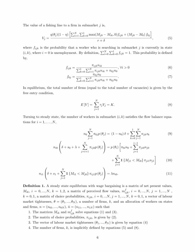
The value of a fishing line to a firm in submarket j is,

Vj =q(θj)(1− η)

[∑Ni=1

∑1k=0 max(Mj0 −Mik, 0)fijk + (Mj0 −M0) f0j

]r + δ

, (5)

where fijk is the probability that a worker who is searching in submarket j is currently in state

(i, k), where i = 0 is unemployment. By definition,∑N

i=0

∑1k=0 fijk = 1. This probability is defined

by,

fijk =πijknik∑1

k=0

∑Ni=1 πijknik + π0jn0

, ∀i > 0 (6)

f0j =π0jn0∑1

k=0

∑Ni=1 πijknik + π0jn0

. (7)

In equilibrium, the total number of firms (equal to the total number of vacancies) is given by the

free entry condition,

E [V ] =N∑j=1

τjVj = K. (8)

Turning to steady state, the number of workers in submarket (i, k) satisfies the flow balance equa-

tions for i = 1, . . . , N ,

n0

N∑j=1

π0jp (θj) = (1− n0) δ +1∑

k=0

N∑j=1

njksk (9)

ni0

δ + s0 + λ+N∑

j=i+1

πij0p (θj)

= p (θi)

[π0in0 +

i−1∑j=1

πji0nj0

+

N∑j=1

1 Mj1 < Mi0πji1nj1]

(10)

ni1

δ + s1 +

N∑j=1

1 Mi1 < Mj0πij1p (θj)

= λni0. (11)

Definition 1. A steady state equilibrium with wage bargaining is a matrix of net present values,

Mik, i = 0, ..., N , k = 1, 2, a matrix of perceived flow values, mfijk, i = 0, ..., N, j = 1, ..., N ,

k = 0, 1, a matrix of choice probabilities, πijk, i = 0, ...N, j = 1, ..., N , k = 0, 1, a vector of labour

market tightnesses, θ = (θ1, ..., θN ), a number of firms, k, and an allocation of workers on states

and firms, n = (n01, ..., n0N ), n = (n11, ..., n1N ) such that

1. The matrices Mik and mfijk solve equations (1) and (3).

2. The matrix of choice probabilities, πijk, is given by (2).

3. The vector of labour market tightnesses (θ1, ..., θN ) is given by equation (4)

4. The number of firms, k, is implicitly defined by equations (5) and (8).

6

5. The allocation of workers on states and firms, n and n solves equations (9)-(11)

Proposition 2. The equilibrium exists.

Proof. The proof is based on a fixed-point argument. We construct a mapping Γ(M, θ, k, n, n) →(M ′, θ′, k′, n′, n′) where all the elements are bounded below by 0 and above by some constant Smax

and that θj∀j and k are bounded below by a constant Smin. Given that the bounds don’t bind, the

mapping goes as follows

1. Given M and θ, construct mijk from equation (1).

2. Given the matrix mfijk, construct the choice probabilities πijk.

3. Given θand M, and πijk, calculate fijk from (6) and (7), and then V from equation (8).

4. Update θby equation (4), θ′j =τjk∑1

k=0

∑Ni=1 πijknik+π0jn0

.

5. Update k: k′ = kV/K.

6. Update n, n:

n′0

N∑j=1

π0jp (θj) = (1− n0) δ +

1∑k=0

N∑j=1

njksk (12)

n′i0

δ + s0 + λ+

N∑j=i

πij0p (θj)

= p (θi)

π0in0 +

i∑j=1

πji0nj0 +

N∑j=1

1 Mj1 < Mi0πji1nj1

(13)

n′i1

δ + s1 +N∑j=1

1 Mi1 < Mj0πij1p (θj)

= λni0. (14)

If the upper or the lower bound binds for a variable, then the variable is equal to the bound.

Given the lower bound on k and θi, it follows by construction that the mapping is continuous.

Hence it follows from Brouwer’s fix-point theorem that the mapping has a fixed point, which we de-

note by (M∗, θ∗, k∗, n∗, n∗). By construction, the fix-point satisfies all the equilibrium requirements

provided that bounds don’t bind. Hence we only have to show that the bounds don’t bind.

In any equilibrium constellation, θj < τjk for all i (the tightness obtained obtained if all workers

search in market j. Hence as k → 0, θj → 0 for all j, and hence V → ∞ (one can show that Vj

goes to infinity for all j). Hence there exists a value Smin k such that V > K for all k ≤ Smin k. Let

tmin = min[τ1, ..., τn]. Define Smin = Smin kτmin. By construction, the lower bound does not bind

at the fixed point neither for k∗ nor θ∗j , j = 1, ..., n.

An upper bound for the profit of a firm is yN(r+δ)k (the net present value of a firm of type n that

employs 1/k workers). Hence an upper bound on k is kmax = yN(r+δ)K . Mik is bounded above by

yn/r. We have only left to show that θj is bounded. For any µthis follows from the fact that all

πijare strictly positive, so that the denominator in (4) is strictly positive (since k is bounded by

km).

We want to look at the limit properties of the model. Consider first the equilibrium of the

7

model when µ→∞. In this case, (2) implies that the probability that a worker goes to submarket

j is equal to τj . Hence the worker has the same probability of meeting any firm, and search is

random.

Suppose then that µ → 0. In the limit, the worker will go to job market j if and only if

this submarket maximizes his return from search. Let Iik denote the set of submarkets that a

worker in state i, k searches to. Then for all j ∈ Iik, Mijk = maxlMikl. By definition it follows

that πijk = 0 iff j /∈ Iijk. If Iijk contains a single element j∗, then πij∗k = 1. The definition

of equilibrium is as before, except that requirement 2 is replaced by the requirement that for all

j ∈ Iik,Mijk = maxlMikl (note that the the reduction in the number of variables is exactly equal

to the reduction in the number of equations).

We say that a state i, k is inferior to another state i′, k′ if Mik < Mi′k′ . We can then show the

following

Lemma 3. The limit economy exists. Furthermore, if i, k is inferior to i′,k’ , then the largest

element in Ii,k is smaller than or equal to the smallest element in Ii′,k′.

The existence proof follows the same lines as above, and is omitted for now. The second part

of the lemma states that the equilibrium leans towards a job ladder. The higher is the current

state (higher NPV income), the higher submarkets the agent searches for. This follows from a

single-crossing property of the indifference curves of agents in different states: the higher is the

current npv income, the more “patient” is the agent, in the sense of being more willing to wait to

obtain a higher wage offer. Submarkets with high firm types offer higher wages and longer queues

(lower job finding rates). Hence, if a worker in a low state ( is indifferent between submarket j and

j + 1, a worker in a higher state will strictly prefer submarket j + 1. The details of the proof is

omitted for now, but follows the lines of the proof of the maximum separation result in Garibaldi,

Moen and Sommervoll (2016).

It follows that as long as each submarket attracts workers of one type (that is, in one particular

state) only, the equilibrium with µ = 0 is identical to the competitive search equilibrium with

on-the-job search derived in Garibaldi, Moen and Sommervoll. If some submarkets attract more

than one worker type, search is still fully directed, but not identical to the competitive search

equilibrium. The reason is that in competitive search equilibrium, different submarkets would

emerge for different worker types that search for the same firm type, and the different submarkets

would have different labor market tightnesses.

In Garibaldi, Moen and Sommervoll, it is shown that with a continuum of firm types, the job

ladder is strict, in the sense that firms of a given type will attract only one type of workers. We

conjecture that this is also the case in our model with bargaining. Furthermore, we conjecture that

as the measure of firms of each type goes to zero, the equilibrium with wage bargaining and µ=0

converges to the competitive search equilibrium (with for instance welfare or job-to-job flows as

metric).

8

3 Specification and solution algorithm

3.1 Specification

Let the matching function in a submarket be Cobb-Douglas, M(s, v) = Asαv1−α. The worker meets

a vacancy at rate p (θ) = M (s, v) /s = m (θ) = Aθ1−α. Hence, p (θ) = Aθ1−α and q (θ) = Aθ−α.

3.2 Solution algorithm

1. The solution algorithm looks to find a fixed point in a mapping of (θ, k) into itself, (θ(m+1), k(m+1)) =

Tθk(θ(m), k(m)).

2. The mapping Tθk is determined as,

3. Take input (θ(m), k(m)).

4. Solve for(m(m),M (m), π(m)

)for given θ(m) using equation systems (1), (3), and (2).

(a) This equation system is solved as fixed point search M∗ = TMM∗.

i. Make a guess, M (s,m).

ii. Solve for m(s,m) using equation (1) - uses M (s,m) and θ(m).

iii. Solve for π(s,m) using equation (2) - uses m(s,m).

iv. Solve for M (s+1,m) using equations (3) - uses θ(m) and π(s,m).

A. This step uses that M can be written as a contraction mapping,

Mik=yi + (δ + sk)M0 + λMi1 +

∑j=1 πijkp (θj) ηmax [Mj0,Mik]

r + δ + sk + λ+∑

j=1 πijkp (θj) η

M0 =y0 +

∑j=1 πijkp (θj) ηMj0

r +∑

j=1 π0jp (θj) η

Thus, simply iterate until convergence to obtain solution. This happens to be

quite fast.

v. loop back to step i with M (s+1,m) as input. Continue to iterate until convergence...

no convergence guaranteed.

(b) In practice, it is faster if the algorithm does not iterate for a full solution of this system

in each (m) iteration.

5. Solve for n(m) as the solution to the linear equation system in equations (9)-(11) taking as

given π(m), M (m) and θ(m).

6. Solve for(θ(m+1), k(m+1)

)as the solution to equations (4) and (8).

9

(a) This step uses a speed up from the Cobb-Douglas formulation. We have that q(θ) = θ−α.

Define,

θ(m)j =

τj∑1k=0

∑Ni=1 π

(m)ijk n

(m)ik + π

(m)0j n

(m)0

.

With this, the free entry condition can then be written as,

k−αN∑j=1

τj θ−αj (1− η)

[∑Ni=1

∑1k=0 max(Mj0 −Mik, 0)fijk + (Mj0 −M0) f0j

]r + δ

= K.

Hence,

k(m+1) =

N∑j=1

τj

(θ(m)j

)−α(1− η)

[∑Ni=1

∑1k=0 max(M

(m)j0 −M

(m)ik , 0)fijk +

(M

(m)j0 −M

(m)0

)f0j

]K (r + δ)

1/α

.

And with this, it immediately follows that,

θ(m+1)j = θ

(m)j k(m+1).

7. With(θ(m+1), k(m+1)

)loop back to step 3. Repeat to convergence.

3.3 Simulation

A worker i’s history consists of a sequence of spells γil, wil, jil, kilLil=1, where γ is the duration, w

is the wage, jil is the firm type of the spell and kil is the layoff rate state. Denote by hjk the hazard

of spell with a j type firm and layoff rate state k. Conditional on an employment spell, j > 0, the

spell hazard is given by

hjk = λ (1− k) + δ + sk +

N∑j′=1

πjj′kp(θj′)1[Mjk < Mj′0

].

If the spell is an unemployment spell, j = 0, the spell is (where the layoff state notation is sup-

pressed),

h0 =N∑j′=1

π0j′p(θj′).

10

Denote by ηjj′kk′ the transition conditional probability that the state of the next spell is (j′, k′)

given that the current spell is state (j, k). It follows directly that,

ηjj01 =λ

hj0, ∀j > 0

ηj0k =δ + skhjk

, ∀j > 0, k ∈ 0, 1

ηjj′kk =πjj′kp(θj′)1

[Mjk < Mj′0

]hjk

, ∀j, j′ > 0, k ∈ 0, 1

η0j =π0j′p(θj′)

h0, ∀j > 0,

and ηjj′kk′ = 0 for all other (j, j′, k, k′) combinations.

The simulation initializes by steady state njk. Thus, from this distribution draw an initial state

for worker i. Then simulate the duration γil ∼ Exp(hjilkil). The state of the next spell is then

drawn according to ηjj′kk′ . Let the length of the simulated panel of workers be T periods. Stop

simulating spells for worker i when∑Li

l=1 γil > T . Let there be I workers in the panel.

4 Estimation

The estimation is based on MEE data meaning we observe mobility patterns close to perfectly.

Specifically, write a worker’s employment history as a series of spells Xi = γil, φilLil=1 where γil is

worker i′s, l’th spell duration and φil is the firm id of the l’th spell. The last spell is necessarily

right censored meaning that the duration of the spell is greater than γiLi and we do not know the

destination firm. A nonemployment spell is associated with φil = 0.

In the model there are N submarkets with a single firm type in each market. This suggests a

simple discrete firm classification as in Bonhomme et al. (2015) and Lentz et al. (2016). There are

J firms and each firm has a type that is drawn from the set j ∈ 1, 2, . . . , N.

4.1 The mobility likelihood for a known firm classification

To start with, suppose we have a known firm classification J = j1, j2, . . . , jJ. Denote by jil =

φ(i, l) the firm type that worker i is matched with in her l′th spell. Denote the job spell hazards

conditional on firm type and layoff rate state by hj0 = δ + s0 + λ +∑N

j′=j+1 πjj′0p(θj′)

and

hj1 = δ + s1 +∑N

j′=1 1Mj1 < Mj′0

πjj′1p

(θj′). The likelihood of the data is based on the

spell duration probability and the origin firm type conditional probability distribution over the

destination firm type. The destination firm distribution depends on the layoff state. Therefore, we

must condition on the layoff state at the end of the spell.

Consider first the probability that a spell ends at duration γ. This probability can be split into

the sum of the joint probabilities that the spell ends at duration γ and that the worker’s layoff

state at duration γ is kγ = 0, plus the joint probability that the spell ends at duration γ and that

11

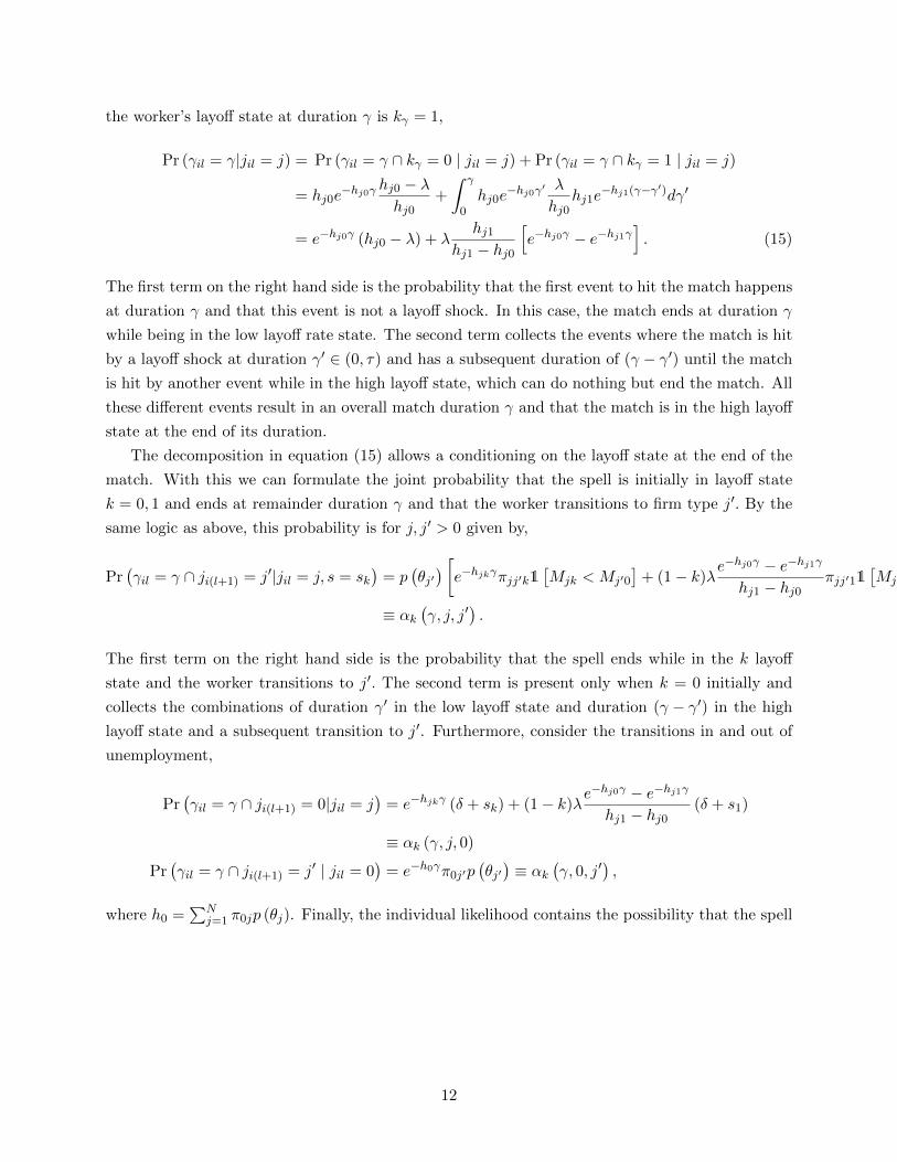
the worker’s layoff state at duration γ is kγ = 1,

Pr (γil = γ|jil = j) = Pr (γil = γ ∩ kγ = 0 | jil = j) + Pr (γil = γ ∩ kγ = 1 | jil = j)

= hj0e−hj0γ

hj0 − λhj0

+

∫ γ

0hj0e

−hj0γ′ λ

hj0hj1e

−hj1(γ−γ′)dγ′

= e−hj0γ (hj0 − λ) + λhj1

hj1 − hj0

[e−hj0γ − e−hj1γ

]. (15)

The first term on the right hand side is the probability that the first event to hit the match happens

at duration γ and that this event is not a layoff shock. In this case, the match ends at duration γ

while being in the low layoff rate state. The second term collects the events where the match is hit

by a layoff shock at duration γ′ ∈ (0, τ) and has a subsequent duration of (γ − γ′) until the match

is hit by another event while in the high layoff state, which can do nothing but end the match. All

these different events result in an overall match duration γ and that the match is in the high layoff

state at the end of its duration.

The decomposition in equation (15) allows a conditioning on the layoff state at the end of the

match. With this we can formulate the joint probability that the spell is initially in layoff state

k = 0, 1 and ends at remainder duration γ and that the worker transitions to firm type j′. By the

same logic as above, this probability is for j, j′ > 0 given by,

Pr(γil = γ ∩ ji(l+1) = j′|jil = j, s = sk

)= p

(θj′) [e−hjkγπjj′k1

[Mjk < Mj′0

]+ (1− k)λ

e−hj0γ − e−hj1γ

hj1 − hj0πjj′11

[Mj1 < Mj′0

]]≡ αk

(γ, j, j′

).

The first term on the right hand side is the probability that the spell ends while in the k layoff

state and the worker transitions to j′. The second term is present only when k = 0 initially and

collects the combinations of duration γ′ in the low layoff state and duration (γ − γ′) in the high

layoff state and a subsequent transition to j′. Furthermore, consider the transitions in and out of

unemployment,

Pr(γil = γ ∩ ji(l+1) = 0|jil = j

)= e−hjkγ (δ + sk) + (1− k)λ

e−hj0γ − e−hj1γ

hj1 − hj0(δ + s1)

≡ αk (γ, j, 0)

Pr(γil = γ ∩ ji(l+1) = j′ | jil = 0

)= e−h0γπ0j′p

(θj′)≡ αk

(γ, 0, j′

),

where h0 =∑N

j=1 π0jp (θj). Finally, the individual likelihood contains the possibility that the spell

12

is right censored,

Pr (γil > γ | jil = j) = e−hjkγ + (1− k)

∫ γ

0hj0e

−hj0γ′ λ

hj0e−hj1(γ−γ′)dγ′

= e−hjkγ + (1− k)λ

hj1 − hj0

[e−hj0γ − e−hj1γ

]≡ αk(γ, j)

Pr (γil > γ | jil = 0) = e−h0γ ≡ αk(γ, 0).

Initialize the likelihood by steady state. That is, the worker is initially observed in submarket

j = 0, 1, . . . , L. Then the probability of this observation is Pr (ji1 = j) = nj , where nj = nj0 + nj1

for any j > 0. With this, the likelihood for a given set of model parameters Ω and worker i’s

mobility pattern for Li > 1 is,

Li (Xi,Ω) = α(γi1, ji1, ji2)α0(γiLi , jiLi)

Li−1∏l=2

α0(γil, jil, ji(l+1))

where,

α(γ, j, j′

)=

nj0α0 (γ, j, j′) + nj1α1 (γ, j, j′) if j > 0

n0αk (γ, 0, j) if j = 0.

For Li = 1 worker i’s likelihood simplifies to,

Li (Xi,Ω) = α(γi1, ji1),

where,

α (γ, j) =

nji10α0(γi1, ji1) + nji11α1(γi1, ji1) if j > 0

n0αk (γ, 0) if j = 0.

The total log likelihood of the data and the given firm classification is,

L (Ω, p | J , X) =

I∑i=1

lnLi (Xi, θ) . (16)

4.1.1 A smoothed likelihood

The likelihood function in equation (16) can be irregular in Ω in that the model may consider moves

between particular submarkets zero likelihood. Of course for the true Ω this does not happen, but

it does pose a practical problem in the search for the maximum. For the purpose of smoothing the

likelihood, consider that the firm classification is measured with noise. Specifically let a(j, j′) be

the probability that the firm truly belongs to submarket j given that it is measured to belong to j′.

13

Hence,∑L

j=1 a(j, j′) = 1. In the next section, we consider a firm specific posterior over the type of

the firm. For now, the measurement error serves the technical purpose of smoothing the likelihood

function. For this purpose, consider the specification,

a(j, j′) ∝ (1 + (∣∣j − j′∣∣+ ε)ρ)−1,

where ρ > 0. For ρ → ∞ one obtains the likelihood in equation (16). With this, denote by

αk (γ, j, j′) the probability that a spell that is initially in layoff state k has remainder duration γ

with a firm that is observed to be in submarket j and moves to another firm that is observed in

submarket j′. For the case where j, j′ > 0 it follows that,

αk(γ, j, j′

)=

L∑i=1

L∑i′=1

a(i, j)a(i′, j′)αk(γ, i, i′).

Similarly,

αk (γ, j) =

L∑i=1

a(i, j)αk(γ, i)

α(γ, j, j′

)=

L∑i=1

L∑i′=1

a(i, j)a(i′, j′)α(γ, i, i′)

α(γ, 0, j′

)=

L∑i′=1

a(i′, j′)α(γ, 0, i′)

αk (γ, 0, j) = )L∑i=1

a(i, j)αk(γ, 0, i)

αk (γ, j, 0) = )L∑i=1

a(i, j)αk(γ, i, 0).

With this the smoothed likelihood can be written as,

Li (Xi,Ω|ρ) = α(γi1, ji1, ji2)α0(γiLi , jiLi)

Li−1∏l=2

α0(γil, jil, ji(l+1)).

And the total log likelihood is,

L (Ω | J , X, ρ) =

I∑i=1

ln Li (Xi, θ|ρ) . (17)

The following shows plots of basic performance of the likelihood in recovering the true param-

eters based on simulated data from the model.

14

Figure 1: Partial identification on simulated data

A5 6 7 8 9 10 11 12 13 14 15

log(

Like

lihoo

d)

#105

-4

-3.5

-3

-2.5

-2

-1.5

-1

-0.5

0

0.5

Profiled Likelihood - A

; = 1; = 2;=5;=10A

2

0.1 0.12 0.14 0.16 0.18 0.2 0.22 0.24 0.26 0.28 0.3

log(

Like

lihoo

d)

#104

-3

-2.5

-2

-1.5

-1

-0.5

0

0.5

1Profiled Likelihood - 2

; = 1; = 2;=5;=102

K30 32 34 36 38 40 42 44 46 48 50

log(

Like

lihoo

d)

-20000

-18000

-16000

-14000

-12000

-10000

-8000

-6000

-4000

-2000

0

2000Profiled Likelihood - K

; = 1; = 2;=5;=10K

6

0.1 0.12 0.14 0.16 0.18 0.2 0.22 0.24 0.26 0.28 0.3

log(

Like

lihoo

d)

#104

-3

-2.5

-2

-1.5

-1

-0.5

0

0.5

1Profiled Likelihood - 6

; = 1; = 2;=5;=106

7

4 6 8 10 12 14 16

log(

Like

lihoo

d)

-200

-150

-100

-50

0

50

100

150

200Profiled Likelihood - 7

; = 1; = 2;=5;=107

s10.05 0.06 0.07 0.08 0.09 0.1 0.11 0.12 0.13 0.14 0.15

log(

Like

lihoo

d)

#104

-3

-2.5

-2

-1.5

-1

-0.5

0

0.5Profiled Likelihood - s0 - Zoomed

; = 1; = 2;=5;=10s

0

15

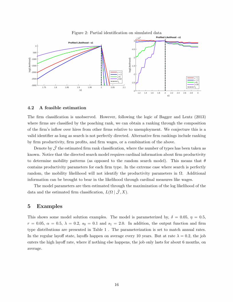
Figure 2: Partial identification on simulated data

s11.75 1.8 1.85 1.9 1.95 2 2.05 2.1

log(

Like

lihoo

d)

-3000

-2500

-2000

-1500

-1000

-500

0

Profiled Likelihood - s1

; = 1; = 2;=5;=10s

1

s11.2 1.4 1.6 1.8 2 2.2 2.4 2.6 2.8 3

log(

Like

lihoo

d)

#105

-3

-2.5

-2

-1.5

-1

-0.5

0

Profiled Likelihood - s1

; = 1; = 2;=5;=10s

1

4.2 A feasible estimation

The firm classification is unobserved. However, following the logic of Bagger and Lentz (2013)

where firms are classified by the poaching rank, we can obtain a ranking through the composition

of the firm’s inflow over hires from other firms relative to unemployment. We conjecture this is a

valid identifier as long as search is not perfectly directed. Alternative firm rankings include ranking

by firm productivity, firm profits, and firm wages, or a combination of the above.

Denote by J the estimated firm rank classification, where the number of types has been taken as

known. Notice that the directed search model requires cardinal information about firm productivity

to determine mobility patterns (as opposed to the random search model). This means that θ

contains productivity parameters for each firm type. In the extreme case where search is perfectly

random, the mobility likelihood will not identify the productivity parameters in Ω. Additional

information can be brought to bear in the likelihood through cardinal measures like wages.

The model parameters are then estimated through the maximization of the log likelihood of the

data and the estimated firm classification, L(Ω | J , X).

5 Examples

This shows some model solution examples. The model is parameterized by, δ = 0.05, η = 0.5,

r = 0.05, α = 0.5, λ = 0.2, s0 = 0.1 and s1 = 2.0. In addition, the output function and firm

type distributions are presented in Table 1 . The parameterization is set to match annual rates.

In the regular layoff state, layoffs happen on average every 10 years. But at rate λ = 0.2, the job

enters the high layoff rate, where if nothing else happens, the job only lasts for about 6 months, on

average.

16

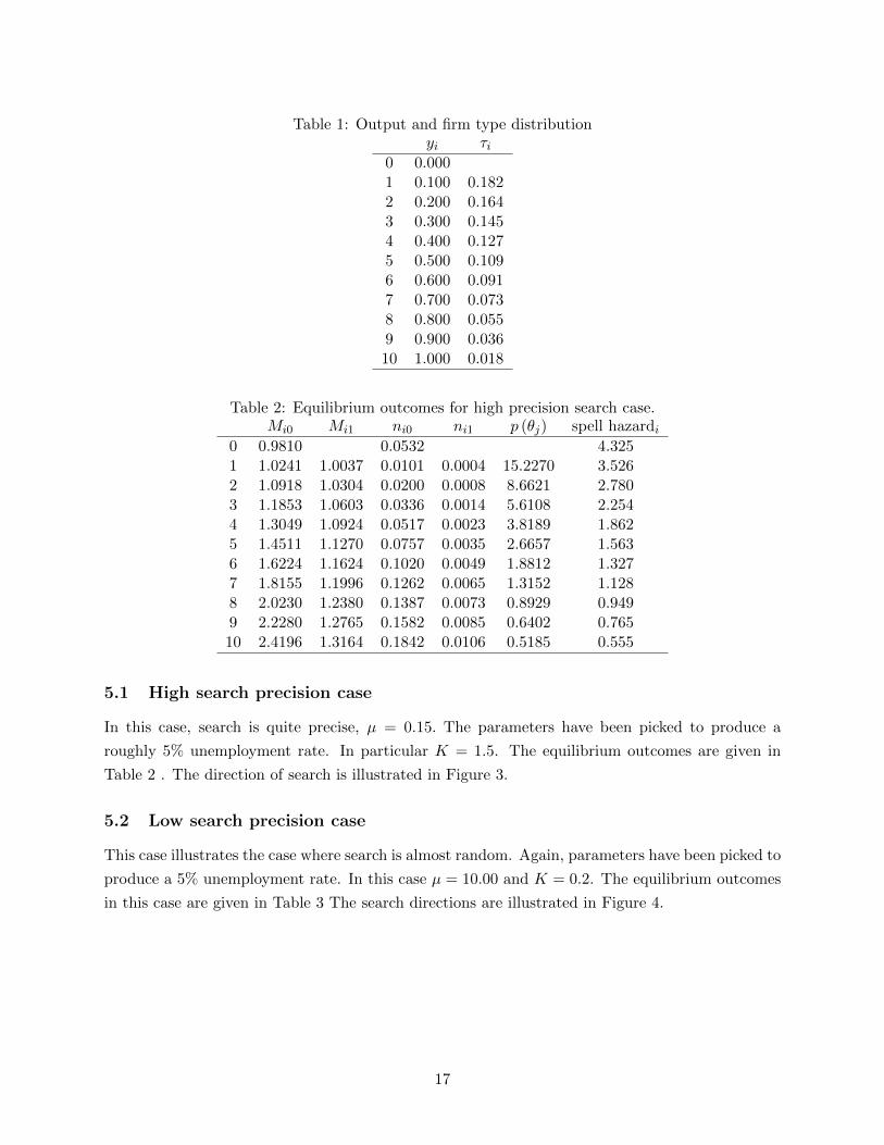
Table 1: Output and firm type distributionyi τi

0 0.0001 0.100 0.1822 0.200 0.1643 0.300 0.1454 0.400 0.1275 0.500 0.1096 0.600 0.0917 0.700 0.0738 0.800 0.0559 0.900 0.03610 1.000 0.018

Table 2: Equilibrium outcomes for high precision search case.Mi0 Mi1 ni0 ni1 p (θj) spell hazardi

0 0.9810 0.0532 4.3251 1.0241 1.0037 0.0101 0.0004 15.2270 3.5262 1.0918 1.0304 0.0200 0.0008 8.6621 2.7803 1.1853 1.0603 0.0336 0.0014 5.6108 2.2544 1.3049 1.0924 0.0517 0.0023 3.8189 1.8625 1.4511 1.1270 0.0757 0.0035 2.6657 1.5636 1.6224 1.1624 0.1020 0.0049 1.8812 1.3277 1.8155 1.1996 0.1262 0.0065 1.3152 1.1288 2.0230 1.2380 0.1387 0.0073 0.8929 0.9499 2.2280 1.2765 0.1582 0.0085 0.6402 0.76510 2.4196 1.3164 0.1842 0.0106 0.5185 0.555

5.1 High search precision case

In this case, search is quite precise, µ = 0.15. The parameters have been picked to produce a

roughly 5% unemployment rate. In particular K = 1.5. The equilibrium outcomes are given in

Table 2 . The direction of search is illustrated in Figure 3.

5.2 Low search precision case

This case illustrates the case where search is almost random. Again, parameters have been picked to

produce a 5% unemployment rate. In this case µ = 10.00 and K = 0.2. The equilibrium outcomes

in this case are given in Table 3 The search directions are illustrated in Figure 4.

17

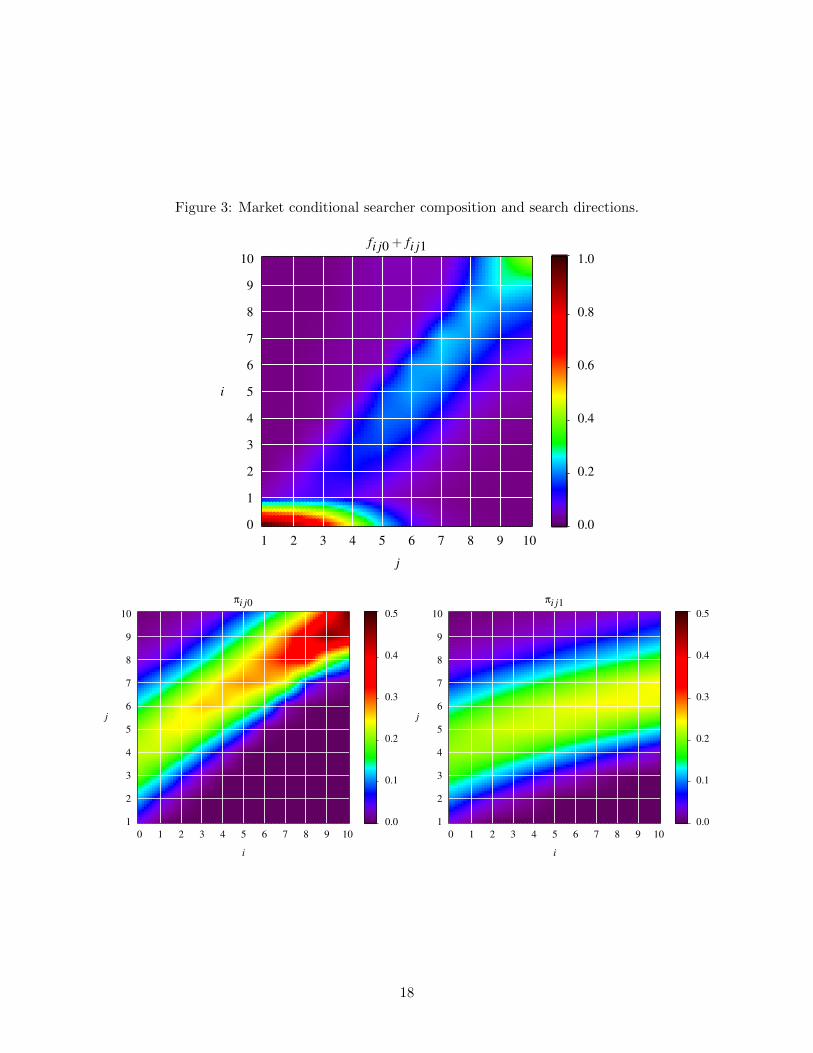
Figure 3: Market conditional searcher composition and search directions.

1 2 3 4 5 6 7 8 9 100

1

2

3

4

5

6

7

8

9

10

0.0

0.2

0.4

0.6

0.8

1.0fi j0 + fi j1

j

i

0 1 2 3 4 5 6 7 8 9 101

2

3

4

5

6

7

8

9

10

0.0

0.1

0.2

0.3

0.4

0.5πi j0

i

j

0 1 2 3 4 5 6 7 8 9 101

2

3

4

5

6

7

8

9

10

0.0

0.1

0.2

0.3

0.4

0.5πi j1

i

j

18

Figure 4: Market conditional searcher composition and search directions (high µ).

1 2 3 4 5 6 7 8 9 100

1

2

3

4

5

6

7

8

9

10

0.00

0.05

0.10

0.15

0.20

0.25fi j0 + fi j1

j

i

0 1 2 3 4 5 6 7 8 9 101

2

3

4

5

6

7

8

9

10

0.00

0.04

0.08

0.12

0.16

0.20πi j0

i

j

0 1 2 3 4 5 6 7 8 9 101

2

3

4

5

6

7

8

9

10

0.00

0.04

0.08

0.12

0.16

0.20πi j1

i

j

19

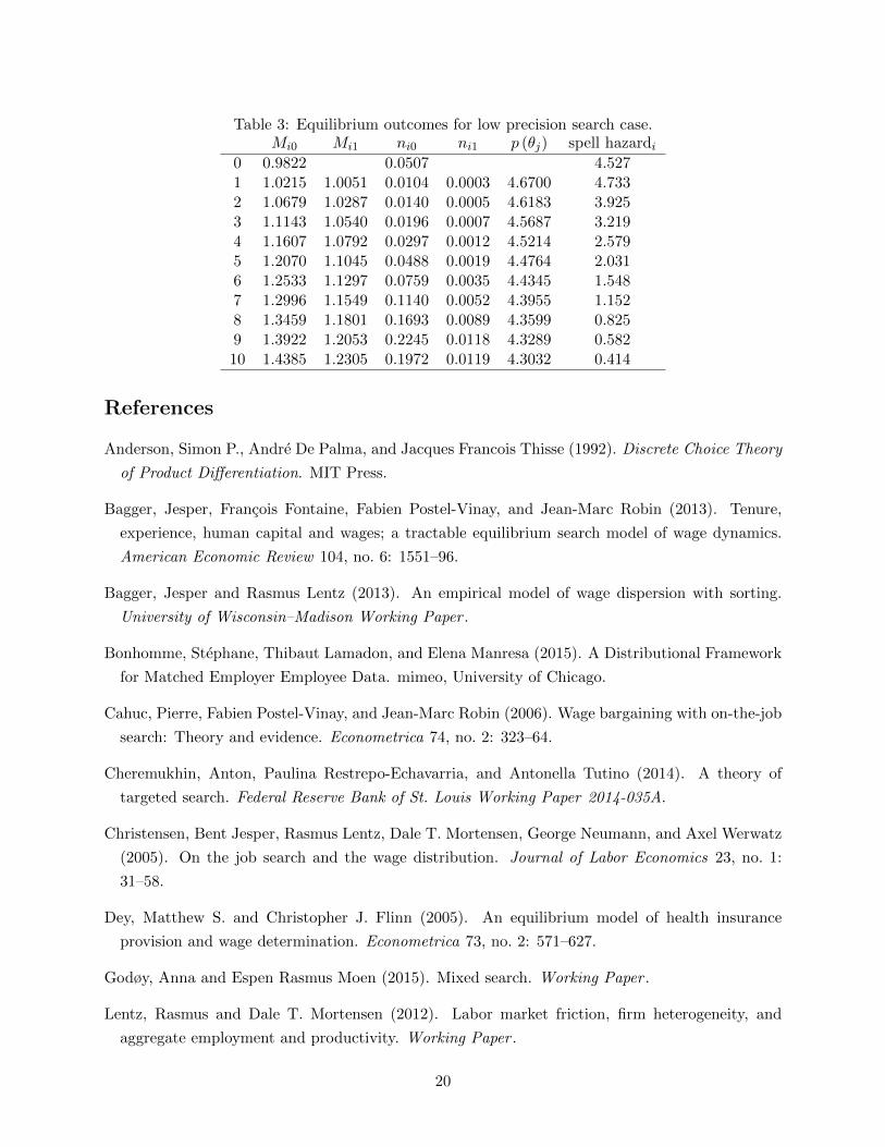
Table 3: Equilibrium outcomes for low precision search case.Mi0 Mi1 ni0 ni1 p (θj) spell hazardi

0 0.9822 0.0507 4.5271 1.0215 1.0051 0.0104 0.0003 4.6700 4.7332 1.0679 1.0287 0.0140 0.0005 4.6183 3.9253 1.1143 1.0540 0.0196 0.0007 4.5687 3.2194 1.1607 1.0792 0.0297 0.0012 4.5214 2.5795 1.2070 1.1045 0.0488 0.0019 4.4764 2.0316 1.2533 1.1297 0.0759 0.0035 4.4345 1.5487 1.2996 1.1549 0.1140 0.0052 4.3955 1.1528 1.3459 1.1801 0.1693 0.0089 4.3599 0.8259 1.3922 1.2053 0.2245 0.0118 4.3289 0.58210 1.4385 1.2305 0.1972 0.0119 4.3032 0.414

References

Anderson, Simon P., Andre De Palma, and Jacques Francois Thisse (1992). Discrete Choice Theory

of Product Differentiation. MIT Press.

Bagger, Jesper, Francois Fontaine, Fabien Postel-Vinay, and Jean-Marc Robin (2013). Tenure,

experience, human capital and wages; a tractable equilibrium search model of wage dynamics.

American Economic Review 104, no. 6: 1551–96.

Bagger, Jesper and Rasmus Lentz (2013). An empirical model of wage dispersion with sorting.

University of Wisconsin–Madison Working Paper .

Bonhomme, Stephane, Thibaut Lamadon, and Elena Manresa (2015). A Distributional Framework

for Matched Employer Employee Data. mimeo, University of Chicago.

Cahuc, Pierre, Fabien Postel-Vinay, and Jean-Marc Robin (2006). Wage bargaining with on-the-job

search: Theory and evidence. Econometrica 74, no. 2: 323–64.

Cheremukhin, Anton, Paulina Restrepo-Echavarria, and Antonella Tutino (2014). A theory of

targeted search. Federal Reserve Bank of St. Louis Working Paper 2014-035A.

Christensen, Bent Jesper, Rasmus Lentz, Dale T. Mortensen, George Neumann, and Axel Werwatz

(2005). On the job search and the wage distribution. Journal of Labor Economics 23, no. 1:

31–58.

Dey, Matthew S. and Christopher J. Flinn (2005). An equilibrium model of health insurance

provision and wage determination. Econometrica 73, no. 2: 571–627.

Godøy, Anna and Espen Rasmus Moen (2015). Mixed search. Working Paper .

Lentz, Rasmus and Dale T. Mortensen (2012). Labor market friction, firm heterogeneity, and

aggregate employment and productivity. Working Paper .

20

Lentz, Rasmus, Suphanit Piyapromdee, and Jean-Marc Robin (2016). The anatomy of the wage

distribution. Working Paper .

Lise, Jeremy, Costas Meghir, and Jean-Marc Robin (2016). Matching, sorting, and wages. Review

of Economic Dynamics 19, no. 1.

Lise, Jeremy and Jean-Marc Robin (2013). The macro-dynamics of sorting between workers and

firms. Working paper .

Moen, Espen R. (1997). Competitive search equilibrium. Journal of Political Economy 105, no. 2:

385–411.

Postel-Vinay, Fabien and Jean-Marc Robin (2002). Equilibrium wage dispersion with worker and

employer heterogeneity. Econometrica 70, no. 6: 2295–2350.

21