Competitive Liner Shipping Network Design · The paper by Agarwal and Ergun (2008) imposes a weekly...

General rights Copyright and moral rights for the publications made accessible in the public portal are retained by the authors and/or other copyright owners and it is a condition of accessing publications that users recognise and abide by the legal requirements associated with these rights.

Users may download and print one copy of any publication from the public portal for the purpose of private study or research.

You may not further distribute the material or use it for any profit-making activity or commercial gain

You may freely distribute the URL identifying the publication in the public portal If you believe that this document breaches copyright please contact us providing details, and we will remove access to the work immediately and investigate your claim.

Downloaded from orbit.dtu.dk on: Jun 05, 2020

Competitive Liner Shipping Network Design

Karsten, Christian Vad; Brouer, Berit Dangaard; Pisinger, David

Publication date:2015

Document VersionPublisher's PDF, also known as Version of record

Link back to DTU Orbit

Citation (APA):Karsten, C. V., Brouer, B. D., & Pisinger, D. (2015). Competitive Liner Shipping Network Design. DTUManagement Engineering.

https://orbit.dtu.dk/en/publications/219a8567-227d-4cc2-94f8-ec99fd6f0f96


Management Science DTU Management Engineering

Christian Vad Karsten Berit Dangaard Brouer David Pisinger 10.2015


Christian Vad Karsten, Berit Dangaard Brouer, and David PisingerDTU Management Engineering,

The Technical University of Denmark

October 26, 2015

Abstract

We present a solution method for the liner shipping network design problem which is acore strategic planning problem faced by container carriers. We propose the first practicalalgorithm which explicitly handles transshipment time limits for all demands. Individualsailing speeds at each service leg are used to balance sailings speed against operational costs,hence ensuring that the found network is competitive on both transit time and cost. We presenta matheuristic for the problem where a MIP is used to select which ports should be insertedor removed on a route. Computational results are presented showing very promising resultsfor realistic global liner shipping networks. Due to a number of algorithmic enhancements, theobtained solutions can be found within the same time frame as used by previous algorithmsnot handling time constraints. Furthermore we present a sensitivity analysis on fluctuationsin bunker price which confirms the applicability of the algorithm.

1 Introduction

Given a fleet of container vessels and a selection of ports, the classical Liner Shipping NetworkDesign Problem (LSNDP) constructs a set of scheduled routes (services) with a fixed frequencyfor container vessels to provide transport for containers worldwide (Brouer et al., 2014a). Thispaper presents the Competitive Liner Shipping Network Design Problem (CLSNDP) extending theclassical LSNDP to consider level of service, i.e. the transit time provided for a given cargo as wellas the transportation cost charged. These two parameters are the main concern for customers, andhence they are crucial parameters for designing competitive networks.

The classical LSNDP is offset in the main objective of the carrier; to maximize profit through therevenues gained from container transport taking into account the fixed cost of deploying vessels andthe variable cost related to the operation of the services. The opposing objectives of the customerand the carrier represents an inherent trade-off in the design of a liner shipping network. Minimizingthe cost of the network will provide low freight rates, but are likely to result in prolonged transittimes as shown by Karsten et al. (2015a). On the other hand, designing a network to minimizetransit times is likely to result in a very costly network favoring direct connections at high sailingspeeds.

The models for the classical LSNDP differ on two traits. First, the ability to model and chargetransshipments between services. Containers are often not transported directly from their port oforigin to their port of destination, and hence it is important to be able to handle the time andcost of transshipments. Second, models differ on requiring a fixed frequency of service or providingflexibility in the frequency. A service is cyclic but may be non-simple, that is, ports can be visitedmore than once. In this model we allow a single port to be visited twice, yielding a so-calledbutterfly route.

1

1 INTRODUCTION 2

The paper by Agarwal and Ergun (2008) imposes a weekly frequency of service and allows fortransshipment, but the model cannot cater for the handling cost associated with transshipments.The paper by Alvarez (2009) can cater for transshipment and transshipment costs (except withinbutterfly services) and allows for flexible frequencies of service. In Reinhardt and Pisinger (2012)each vessel is treated separately allowing flexible frequencies, and the model allows for transship-ment costs also on butterfly routes. Brouer et al. (2014a) provides an analysis of the real liferequirements and present a reference model for the classical LSNDP. The model is offset in Alvarez(2009) accounting correctly for transshipments on all services and allowing both flexible and fixedfrequencies. The above models are all variants of specialized capacitated network design problems.

Meng et al. (2014); Christiansen and Fagerholt (2011); Christiansen et al. (2013) providebroader reviews of recent research on routing and scheduling problems within liner shipping. In theliterature several papers extend the classical LSNDP e.g. by incorporating intermodal considera-tions (Liu et al., 2014) or aiming to narrow the definition of service (Plum et al., 2014). However,it is generally acknowledged that considering level of service is the most important extension tothe classical LSNDP because it is the decisive factor in designing a competitive network (Alvarez,2012; Brouer et al., 2014a). Two approaches for considering level of service has been suggested inthe literature. The first method is to include inventory cost in a multi-criteria objective functionas seen in Alvarez (2012). Inventory cost is primarily a concern to the shipper and the idea ofintroducing it for the carrier is to ensure that longer transit times will result in lower freight rates.However, the bilinear expression proposed by Alvarez (2012) is not computationally tractable. An-other approach is to impose restrictions on the allowed transit times for each container. The ideahere is that the carrier needs to provide competitive transit times in a market of several players.Wang and Meng (2014) introduce deadlines on cargo in a non-linear, non-convex mixed-integerprogramming (MIP) formulation of a LSNDP. A drawback of this formulation is that it cannotcater for transshipments of cargo which is the backbone of global liner shipping networks. RecentlyBrouer et al. (2015) presented a capacitated multi-commodity network design formulation that im-poses transit time restrictions while still allowing transshipments between services and Karstenet al. (2015a) showed that time restricted multi-commodity flow problem arising as a sub-problemcan be efficiently solved for a large global shipping network. The CLSNDP in this paper buildupon these contributions.

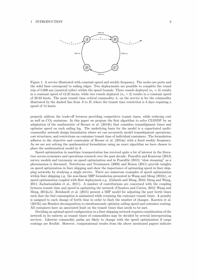
Introducing transit time restrictions is essential in the LSNDP from a customer perspective, butto maintain low fuel (bunker) cost this must be accompanied by modelling the services with variablespeed. Traditionally, models of the LSNDP operate with a constant speed on services althoughvariable speed on each leg is used in practice. In a network with constant speed the most transittime restricted commodity will force the entire service to speed up, and hence increase the bunkerconsumption of the service unnecessarily with a resulting increase in both cost and CO2 emissions.Figure 1 illustrates the problem of maintaining constant speed during the design process. Thecontainer entering at A and leaving at B, kAB , has the tightest transit time requirement amongthe containers currently transported on service s with a transit time restriction of 3 days, whichrequires a speed of 14 knots. This results in a deployment of 2 vessels at a speed of nearly 21knots, because of only two possible deployments with constant speed and the weekly frequencyrequirement imposed. If speed can be determined individually on each sailing leg, 3 vessels canbe deployed with a speed of 14 knots between A and B and a speed of 12 knots on the remainingsailing legs maintaining the weekly frequency but resulting in a significant decrease in the bunkerconsumption (since the bunker consumption is a cubic function of the speed (Brouer et al., 2014a)).The computational results presented in Brouer et al. (2015) support a higher average speed andlow fleet deployment in networks optimized with transit time restrictions and constant speed.

Therefore, the CLSNDP is extending the reference model for LSNDP Brouer et al. (2014a)to consider transit time restrictions coupled with variable speed on each sailing leg in order to

1 INTRODUCTION 3

A B

CD

1000 nm

1000 nm

1500 nm

1500 nm

k

k

k

Figure 1: A service illustrated with constant speed and weekly frequency. The nodes are ports andthe solid lines correspond to sailing edges. Two deployments are possible to complete the roundtrip of 5,000 nm (nautical miles) within the speed bounds: Three vessels deployed (ne = 3) resultsin a constant speed of 12.25 knots, while two vessels deployed (ne = 2) results in a constant speedof 20.83 knots. The most transit time critical commodity, k, on the service is for the commodityillustrated by the dashed line from A to B, where the transit time restriction is 3 days requiring aspeed of 14 knots.

properly address the trade-off between providing competitive transit times, while reducing costas well as CO2 emissions. In this paper we propose the first algorithm to solve CLSNDP by anadaptation of the matheuristic of Brouer et al. (2014b) that considers transshipment times andoptimize speed on each sailing leg. The underlying basis for the model is a capacitated multi-commodity network design formulation where we can accurately model transshipment operations,cost structures, and restrictions on container transit time of individual containers. The formulationadheres to the objective and constraints of Brouer et al. (2014a) with a fixed weekly frequency.As we are not solving the mathematical formulation using an exact algorithm we have chosen toplace the mathematical model in A.

Speed optimization in maritime transportation has received quite a lot of interest in the litera-ture across economics and operations research over the past decade. Psaraftis and Kontovas (2013)survey models and taxonomy on speed optimization and in Psaraftis (2015) “slow steaming” as aphenomenon is discussed. Notteboom and Vernimmen (2009) and Ronen (2011) provide insightson speed optimization in liner shipping and show the importance of optimizing speed in liner ship-ping networks by studying a single service. There are numerous examples of speed optimizationwithin liner shipping e.g. the non-linear MIP formulation presented in Wang and Meng (2012c), orspeed optimization coupled with fleet deployment e.g. (Gelareh and Meng, 2010; Meng and Wang,2011; Zacharioudakis et al., 2011). A number of contributions are concerned with the couplingbetween transit time and speed in optimizing the network (Cheaitou and Cariou, 2012; Wang andMeng, 2012a,b). Reinhardt et al. (2015) present a MIP model for adjusting the port berth timessuch that the fuel consumption is minimized while retaining the customer transit times. A penaltyis assigned to each change of berth time in order to limit the number of changes. Karsten et al.(2015b) use Benders decomposition to simultaneously optimize sailing speed and container routing.All containers have an associated limit on the transit times that needs to be met.

Deciding an optimal speed configuration in a liner shipping network requires consideration of thenetwork in its entirety as transit times of commodities may be decided by several interoperatingservices. Likewise commodity paths are likely to change with the speed optimization if cargoroutings are flexible. However, computational results from the above mentioned papers indicate

2 PROBLEM DESCRIPTION 4

that this is not computationally tractable for revaluation in a large-scale heuristic search. Thematheuristic for the CLSNDP proposed in this paper is considering speed as one of the dimensionsin the solution space and therefore a fast method for optimizing speed is needed. In tramp shippingspeed optimization of an isolated route in the network is optimal. Variable speed for a single shiproute in tramp shipping has been explored in Fagerholt et al. (2009); I. Norstad and Laporte(2011); Hvattum et al. (2013), where the introduction of speed optimization allowing variablespeed on a sail route results in significant fuel savings. In Fagerholt et al. (2009) a MIP witha non-linear objective function depicting the vessels fuel consumption as a function of speed ispresented. The speed optimization problem can be transformed into a directed acyclic graph ifspeeds are discretized and the resulting speed profile is simply a shortest path, which can beefficiently calculated for a directed acyclic graph. The approach by Fagerholt et al. (2009) cannotbe adopted directly, since a liner shipping service will be carrying multiple commodities and hencethe time windows are defined per pickup node. Transforming the problem into a graph wouldresult in node specific time windows accounting for times between every OD pair assigned to theservice, which would require a resource constrained shortest path with a specific resource for everyport in the service. This is unlikely to be efficiently solved. However, we can adapt the non-linearMIP formulation of Fagerholt et al. (2009) to optimize speed on a single service given constraintson the slack time of each commodity currently transported on the service. As a novelty we alsoconsider opportunity cargo not currently transported, as speed optimization may lead to newattractive transport opportunities. The non-linear bunker consumption function is approximatedby a piecewise linear function of the time to sail a given leg and the speed optimization MIP canbe efficiently solved using a standard MIP solver making it suitable to incorporate into a heuristic.Our computational results show that it is tractable to incorporate level of service in the networkdesign process by considering container transit time restrictions and variable speed in a heuristiccontext, and we are able to design profitable networks for scenarios resembling global liner shippingnetworks.

The rest of the article is organized as follows. Section 2 discuss the extensions from the LSNDPto the CLSNDP. Section 3 gives an overview of our solution method and describe the level ofservice implications in detail. Section 4 presents computational results on realistic instances fromthe benchmark suite LINER-LIB before we conclude and discuss future work in Section 5.

2 Problem description

Given a fleet of container vessels and a selection of ports, the CLSNDP constructs a set of servicesto provide transport for containers worldwide. It extends the classical LSNDP to consider levelof service as this is the main concern for the shipper. The CLSNDP we present here is based onthe reference model for the LSNDP presented in Brouer et al. (2014a) which has been extendedin Brouer et al. (2015) to consider transit time restrictions for all commodities, see A for a fulldescription of the model. The primary change in order to accommodate transit time restrictionsinto the model of Brouer et al. (2014a) is to decompose the multi commodity flow problem into apath flow formulation. In the path flow formulation only paths respecting the maximal transit timefor a given commodity are feasible. This extension of the LSNDP with transit time restrictions is anon-compact formulation with integer service variables defining a port call sequence, a vessel type,number of ships and a constant speed, and real path variables for routing the commodities. Astransit times are closely linked to speed, the constant speed needed to accommodate transit timerestrictions will generally be determined by the commodity with the most restrictive transit time.However, it is unnecessary to maintain a high speed throughout the service if this commodity isonly carried on part of the service. Therefore we use service variables that include variable speedby allowing each sailing to take on any speed within the feasible speed interval, while maintaining

3 ALGORITHM 5

a weekly frequency of service. The overall objective of CLSNDP is to maximize profit, however,the extensions potentially results in fuel savings and/or a larger cargo uptake in the network alongwith ensuring a competitive level of service in the network.

The next section provides a broad overview of the algorithm and its components. The overviewincludes the extensions necessary to enable consideration of level of service, namely transit timerestrictions for each individual commodity and optimizing speed on each sailing in the network.Following the overview the extensions will be described in further detail.

3 Algorithm

The proposed matheuristic is based on the algorithm from Brouer et al. (2014b). Since the evalua-tion of the objective function makes it necessary to flow all containers through the network, only alimited number of iterations can be evaluated throughout the search, and therefore it is importantto use a large neighborhood search, combined with a shrewd way of choosing the direction of thesearch.

Algorithm 1 presents high level pseudocode for the overall matheuristic. Initially a solution isconstructed by dividing the available fleet onto services. Subsequently the services are populatedwith port calls following a greedy parallel insertion procedure according to the distance and thetrade volume between ports in the service in line 1. The subsequent search for improved solutionsis guided by a simulated annealing scheme in the while loop of lines 5-25. The primary componentof the matheuristic is a neighbourhood for inserting and removing port calls on a single servicewhich is formulated as an integer program in line 8. The integer program is described in detail inSection 3.1. In order to optimize speed in the network a heuristic method based on a non-linearMIP is applied. The heuristic optimizes the speed of all legs on a single service given the timelimits of cargo currently transported on this service and the time limit of opportunity demands,that are currently rejected due to transit time restrictions. This MIP is called in line 10 afterresolving the multicommodity flow problem in line 9 given the changes to service s. As changesare only made to a single service, the column generation algorithm used is warm started using thetechnique described in Brouer et al. (2014b). The simulated annealing scheme decides whetherthe new solution is accepted in line 12. The reinsertion heuristic in line 18 introduces butterflyports on promising candidate services. The perturbation heuristic in line 23 diversifies the servicecomposition. The two latter heuristics are unchanged to the versions in Brouer et al. (2014b).

3.1 The improvement heuristic with level of service considerations

The integer program described in line 8 of Algorithm 1 is a move operator in a large-scale neigh-borhood search based on altering a single service at a time. The objective of the integer programare estimation functions for changes in the flow of the network and the duration of the servicedue to insertions and removals of port calls. The solution of the integer program provides a setof moves in the composition of port calls and fleet deployment. Flow changes and the resultingchange in the revenue for relevant commodities to the insertion/removal of a port call are estimatedby solving a series of resource constrained shortest path problems considering feasibility of transittime restrictions as well as the cost of transport including transshipments.

Given a total estimated change in revenue of revi and port call cost of ce(s)i Figure 2(a) illustrates

estimation functions for the change in revenue (Θsi ) and duration increase (∆s

i ) for inserting porti into service s controlled by the binary variable γi. The duration controls the number of vesselsneeded to maintain a weekly frequency. Figure 2(b) illustrates the estimation functions for thechange in revenue (Υs

i ) and decrease in duration (Γsi ) for removing port i from service s controlledby the binary variable λi.

3 ALGORITHM 6

A

BγB

ΘsB = revB − ce(s)B

∆sB = 1

C D

F

E γE

ΘsE = revE − ce(s)E

∆sE = 1

G

1

1

1

1

11

1

(a) Blue nodes are evaluated for insertion corresponding to variables γi forthe set of ports in the neighborhood Ns of service s.

A

CλC

ΓsC = 1

Υsc = −revc + ce(s)C

D

F

G

1

1

1

11

1

(b) Red nodes are evaluated for removal corre-sponding to variables λi for the set of current portcalls F s on service s.

Figure 2: Illustration of the estimation functions for insertion and removal of port calls.

3 ALGORITHM 7

Algorithm 1 High Level algorithm for CLSNDP

Require: An instance of the CLSNDP1: Construct an initial solution x using a greedy algorithm2: Set the best known solution x∗ = x3: Set the iteration counter iter = 04: Set the initial temperature temp = temp0

5: while temp > 0.01 AND time < MAXtime do6: for each service s ∈ x do7: x′ ← x \ s8: s′ ← IP (s): improve solution by insertion/removal of port calls on service s9: Resolve cargo flow

10: Optimize speed of each sailing on s′

11: x′ ← x′⋃s′

12: if accept solution according to cooling scheme then13: Set x← x′

14: Possibly update best known solution: x∗ ← x15: iter ← iter + 116: temp← temp · 0.9817: if iter mod 4 = 0 then18: Apply reinsertion heuristic to obtain new solution x′ with promising butterfly routes19: if Solution improves then20: Set x← x′

21: Possibly update best known solution: x∗ ← x22: if iter mod 10 = 0 then23: Apply perturbation to obtain a solution x′ with a different service composition24: Set x← x′

25: Possibly update best known solution: x∗ ← x26: return (x∗)

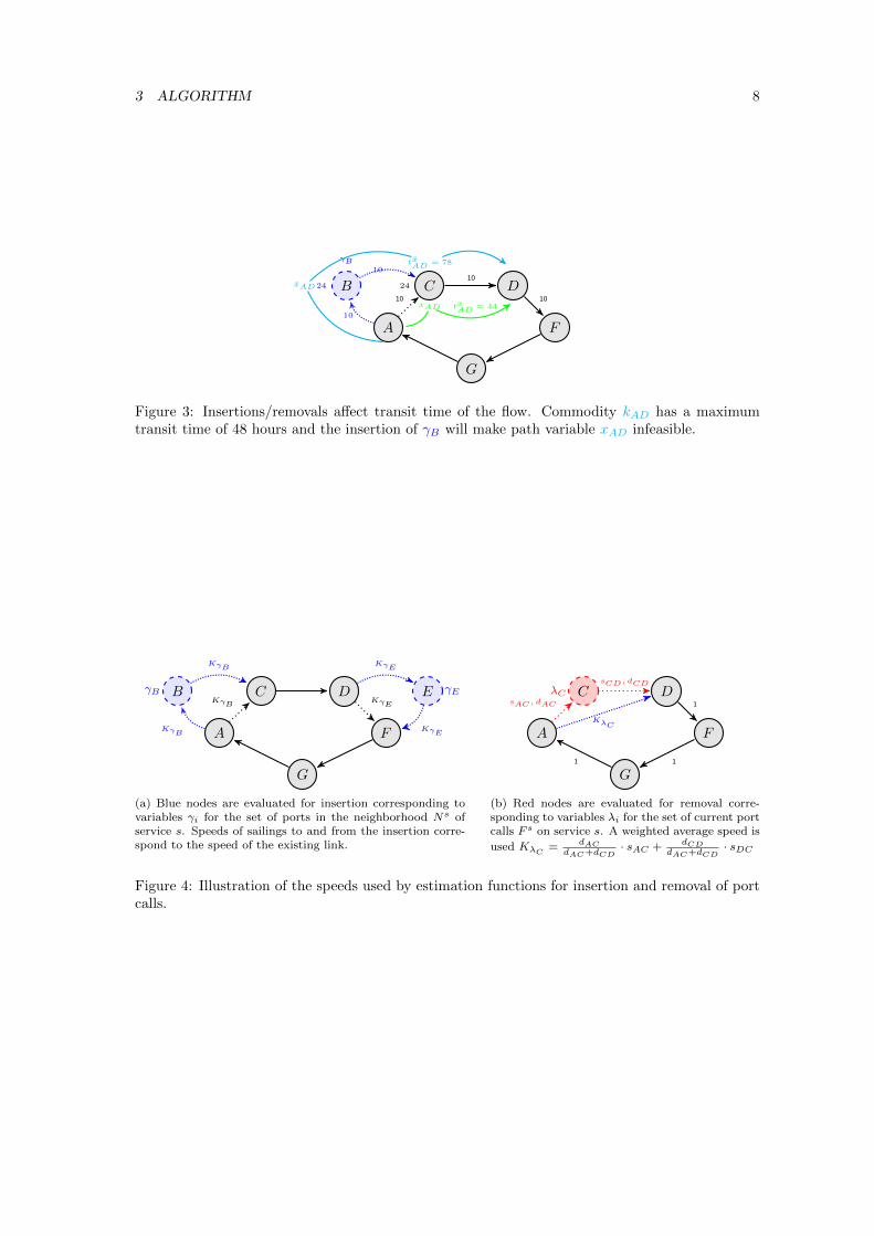
For considering the transit time in the IP, it is necessary to estimate how insertions and removalsof port calls will affect the duration of the existing flow on the service. If an insertion is estimatedto result in exceeding the transit time restriction of existing flow, and there is no possibility ofrerouting the flow on a different path respecting the transit time limits, a loss of revenue canbe expected. The loss is estimated to correspond to the full revenue obtained from the demandquantity. Figure 3 illustrates a case of a path variable in the current basis of the MCF model,which becomes infeasible due to transit time restrictions when inserting port B on its path.

In order to account for the transit time restrictions of the current flow, constraints (8) areadded to the IP and a penalty, ζx corresponding to losing the cargo, is added to the objective ifthe transit time slack for an existing path variable becomes negative. This is handled through thevariable αx, where x refers to a path variable with positive flow in the current solution and sx refersto the current slack time according to the transit time restrictions of the variable. Variable speedis considered in the estimation function for the flow as well as for the estimation of the serviceduration. The speed on the sailings to and from the port evaluated for insertion is estimated tobe equal to the speed sailed between the two ports previously connected and is denoted by theconstant Kγi . Upon evaluating a removal of a port the actual speed of the sailing in question isused to reduce the duration of the service. The constant Kλi expresses the weighted average speedof the current speeds for the sailings entering and leaving the port estimated for removal. Thespeeds used for the estimation functions are illustrated in Figure 4.

3 ALGORITHM 8

A

BxAD

γB

24 C24

txAD = 78

xAD

D

F

G

10

10

10

10

10

txAD = 44

Figure 3: Insertions/removals affect transit time of the flow. Commodity kAD has a maximumtransit time of 48 hours and the insertion of γB will make path variable xAD infeasible.

A

BγB C D

F

E γE

G

KγBKγE

KγE

KγEKγB

KγB

(a) Blue nodes are evaluated for insertion corresponding tovariables γi for the set of ports in the neighborhood Ns ofservice s. Speeds of sailings to and from the insertion corre-spond to the speed of the existing link.

A

CλC D

F

G

sAC, dAC

sCD, dCD

1

11

KλC

(b) Red nodes are evaluated for removal corre-sponding to variables λi for the set of current portcalls F s on service s. A weighted average speed is

used KλC = dACdAC+dCD

· sAC + dCDdAC+dCD

· sDC

Figure 4: Illustration of the speeds used by estimation functions for insertion and removal of portcalls.

3 ALGORITHM 9

For ease of reading, Table 1 gives an overview of additional sets, constants, and variables usedin the IP.

Sets

F s Set of port calls in sNs Set of neighbors (potential port call insertions) of sXs Set of path variables on service s in current flow solution with positive flowNx ⊆ Ns Subset of neighbors with insertion on current path of variable x ∈ Xs

F x ⊆ F s Subset of port calls on current path of variable x ∈ Xs

Li Lock set for port call insertion i ∈ Ns or port call removal i ∈ F s

Constants

Y s Distance of the route associated with sBi Berthing time for port call i ∈ F s isV s Estimated weighted average speed over all sailings on the service sVγi Speed between insertion points on the service sVλi Speed on sailing removed from the service sCe Cost of an additional vessels of class e(s)ne Number of deployed vessels of class e(s) to s in the current solutionMe Number of undeployed vessels of class e in the current solutionIs Maximum number of insertions allowed in sRs Maximum number of removals allowed in s∆si Estimated distance increase if port call i ∈ Ns is inserted in s

Γsi Estimated distance decrease if port call i ∈ F s is removed from sΘi Estimated profit increase of inserting port call i ∈ Ns in sΥi Estimated profit increase of removing port call i ∈ F s from sζx Estimated penalty for cargo lost due to transit timesx Slack time of path variable x

Variables

λi Binary, 1 if port call i ∈ F s is removed from s, 0 otherwiseγi Binary, 1 if port call i ∈ Ns is inserted in s, 0 otherwiseωs Integer, number of vessels added (removed if negative) to sαx Binary, 1 if transit time of path variable x ∈ Xs is violated, 0 otherwise

Table 1: Overview of sets, constants, and variables used in the IP

The objective of the move operator is to maximize the estimated profit increase obtained fromremoving and inserting port calls, accounting for the estimated change of revenue, transshipmentcost, port call cost, and fleet cost.

max∑i∈Ns

Θiγi +∑i∈F s

Υiλi − Ceωs − ζxαx (1)

First, we need to estimate the number of vessels ωs needed on the service s (assuming a weeklyfrequency) after insertions/removals while accounting for the change in the service time given thecurrent weighted average speed on the service V s:

Y s

V s+∑i∈F s

Bi +∑i∈Ns

(∆si

Vγi+Bi

)γi −

∑i∈F s

(ΓsiVλi

+Bi

)λi ≤ 24 · 7 · (ne + ωs) (2)

Next, we must ensure that the solution does not exceed the available fleet of vessels. Note that ωs

does not need to be bounded from below by −ne because it is not allowed to remove all port calls:

ωs ≤Me (3)

3 ALGORITHM 10

Then, a limit on the number of port call insertions and removals is enforced in order to minimizethe error in the computed estimates: ∑

i∈Nsγi ≤ Is (4)∑

i∈F sλi ≤ Rs (5)

Furthermore, the flow estimates are based on cargo flowing to and from a set of related port calls onthe service. The affected ports are placed in a lock set, Li, for insertions and removals respectively,i.e. ports in a lock set cannot be removed to avoid large deviations in the flow estimates:∑

j∈Li

λj ≤ |Li|(1− γi) i ∈ Ns (6)

∑j∈Li

λj ≤ |Li|(1− λi) i ∈ F s (7)

Finally, we need to activate the estimated penalty for lost cargo due to an estimated violation ofthe transit time for the commodity on this particular path:∑

i∈Nx

(∆si

V s+Bi

)γi −

∑i∈Fx

(ΓsiV s

+Bi

)λi − UBαx ≤ sx x ∈ Xs (8)

The domains of the variables are:

λi ∈ 0, 1, i ∈ F s γi ∈ 0, 1, i ∈ Ns αx ∈ 0, 1, x ∈ Xs ωs ∈ Z, s ∈ S

As opposed to the move operator proposed in Brouer et al. (2014b) the change in revenue maybe related to not transporting cargo for which the path duration is estimated to exceed the transittime of the commodity.

3.2 Variable Speed on Service Legs

To include variable speed in the matheuristic (Algorithm 1 line 10) we formulate the speed opti-mization problem as a mixed integer program with a non-linear objective function that can easilybe solved for each service s ∈ S during the iterative search. m is the number of port calls in theround trip of s and m + 1 is the first port of call. The function g(tj,j+1, dj,j+1) represents thebunker consumption from port j to j+1 expressed as a function of sailing time tj,j+1 and distancedj,j+1, which indirectly models the speed vj,j+1. For each service we wish to determine the sailingspeed of each sailing leg which we do by finding the optimal sailing time tj,j+1 between ports jand j + 1. We arrive in port j at time tj and the sailing time must be determined such thatthe weekly frequency of a service is maintained. If the sailing speed is changed significantly it ispossible to add or remove an additional vessel to the service provided that additional vessels areavailable. As a novelty we also consider commodities that are not currently transported but couldbe transported on service s if a sufficient speed increase is profitable. To find the set of candidatecommodities for a service we solve an unconstrained shortest path problem on the residual capacitygraph of the current network for all commodities that are not currently transported. We add theones that have a profitable path through service s to the set but where transit time is then violatedto Kp,s and calculate the potential profit based on the residual capacity (which may be less thanthe demand of a cargo), the cost of the path and the service penalty (which we potentially canavoid). Additionally we keep track of the time decrease needed (corresponding to a speed up) to

3 ALGORITHM 11

Sets

Ks Set of commodities currently transported on s where tok < tdkKs Set of commodities currently transported on s where tok > tdkKp,s Set of commodities that potentially could be transported on s where tok < tdkKp,s Set of commodities that potentially could be transported on s where tok > tdk

Constants

Tmin Time to complete service s at minimum speedtsk Time commodity k currently uses on service s and the possible slack time

between the time of the current path and the overall transit time limit of k

zk Net revenue that will be lost if not transporting the demand k ∈ Ks ∪ Ks

rk Net revenue that can be obtained by transporting all of demand k ∈ Kp,s ∪ Kp,s

tcurs,k Time commodity k ∈ Kp,s ∪ Kp,s currently would spend on service s

tlacks,k Time currently lacking for commodity k ∈ Kp,s ∪ Kp,s

Variables

tj Continuous, arrival time at port jtj,j+1 Continuous, sailing time between ports j and j + 1δe Integer, change in the number of vessels of class e(s) deployed to service sρk Binary, 1 if commodity k will be lost due to transit time violationηk Binary, 1 if commodity k will be available if transit time is reduced

Table 2: Overview of sets, constants, and variables used in the Speed MIP

make the path feasible. The constants, sets and variables used in the model for a specific services ∈ S are summarized in Table 2.

Using this notation, the objective for each service is to minimize the objective function ac-counting for the bunker cost, the expected loss of revenue due to transit times not met and thedeployment cost of additional vessels less the profit from demand that become available for trans-port by adjusting the speed. The objective can be written as:

min

m∑j=1

cBg(tj,j+1, de(s)j,j+1) +

∑Ks∪Ks

zkρk + Ceδe −∑

Kp,s∪Kp,s

rkηk (9)

A number of constraints need to be satisfied: First, we need to set the time for each port on aroute and the sailing time between ports for calculating the bunker consumption:

tj+1 − tj − tj,j+1 ≥ Bj j = 1 . . .m (10)

Next, we decide the number of vessels needed to maintain a weekly frequency on the serviceincluding berthing time for each port call:

tm+1 − 168 · δV = 168 · ne −m∑j=1

Bj (11)

The service time is set by the constraint:

m∑j=1

tj,j+1 = tm+1 (12)

Moreover, we invoke a loss of revenue if the transit times of commodities on board the service sare not met. A separate constraint is necessary for commodities where tok < tdk to account for

4 COMPUTATIONAL RESULTS 12

the total round trip time:

tdk − tok − ρkTmin ≤ tk k ∈ Ks (13)

tdk − tok − ρkTmin + tm+1 ≤ tk k ∈ Ks (14)

Similar constraints allow a service to pick-up additional cargo if speed is increased sufficiently tomake paths for cargo that was previously rejected due to transit time limits:

tdk − tok − (1− ηk)Tmin ≤ tcurs,k − tlacks,k k ∈ Kp,s (15)

tdk − tok − (1− ηk)Tmin + tm+1 ≤ tcurs,k − tlacks,k k ∈ Kp,s (16)

Finally, we need to enforce speed bounds of the vessel class used by service s:

tj,j+1 ≥dj,j+1

vmaxj = 1 . . .m (17)

tj,j+1 ≤dj,j+1

vminj = 1 . . .m (18)

The variable δe is bounded from above by the number of available vessels if the service slows downoverall by adding an additional vessel to the service. The bounds on δe are tightened in order togive a good solution close to the current deployment such that −1 ≤ δV ≤ min1,Me, i.e. it isonly possible to add or remove at most one vessel. The variable domains are:

δe ∈ −1, 0,min1,Me (19)

tj , tj,j+1 ∈ R+ j = 1 . . .m (20)

ρk ∈ 0, 1 k ∈ Ks ∪ Ks (21)

ηk ∈ 0, 1 k ∈ Kp,s ∪ Kp,s (22)

The objective function can be linearized by modeling the bunker consumption as a piecewise linearfunction for each tj,j+1 and the model (9)-(22) can be solved efficiently by a standard mixed integerprogramming solver. We use 100 pieces to accurately model the bunker consumption function(the solution times for the speed optimization problem are generally less than 0.1 seconds in theinstances we have solved in Section 4 and the number of pieces used to aprroximate the objectiveonly has limited impact on this.)

As described earlier, when a service in the network is changed we re-solve the cargo flowingsubproblem using a warmstarting procedure where previously generated columns are used leadingto a very effective solution of the flow problem. It should be noted that solving the speed optimiza-tion for each service separately leads to a sub-optimal configuration of the network as a significantportion of the demands uses more than one service and hence the transit time for each demand isdetermined by more than one service, but as we solve the problem many times for each service aspart of the search procedure large differences can be reduced.

4 Computational Results

The matheuristic was tested on data from the benchmark suite LINER-LIB described in Broueret al. (2014a). The instances can be found at http://www.linerlib.org. Table 3 gives an overviewof the instances. The transit time restrictions have been updated according to the most recentpublished liner shipping transit times for a small number of the origin-destination pairs as describedin Brouer et al. (2015).


Category Instance and description |P | |K| |E|Single- Baltic Baltic sea, Bremerhaven as hub 12 22 2hub WAF West Africa, Algeciras as hub 19 38 2Multi-hub Mediterranean Algeciras, Tangier, and Gioia Tauro as hubs 39 369 3Trade- Pacific Asia and US West Coast 45 722 4lane AsiaEurope Europe, Middle East and Far East regions 111 4000 6World WorldSmall 47 main ports worldwide 47 1764 6

Table 3: The instances of the benchmark suite with indication of the number of ports |P |, thenumber of origin-destination pairs |K|, and the number of vessel classes |E|.

The matheuristic has been coded in C++ and run on a linux system with an Intel(R) Xeon(R)X5550 CPU at 2.67GHz and 24 GB RAM. The algorithm is set to terminate after the time limitsimposed in Brouer et al. (2014a) if the stopping criterion of the embedded simulated annealingprocedure is not fulfilled at the time limit.

We fix the berthing time, Bp to 24 hours for all ports as in Brouer et al. (2014a) and thetransshipment time, ta is fixed to 48 hours for every connection as the concrete time schedule isnot known at this stage. The bunker price is set to $ 600 per ton as in Brouer et al. (2014a). Pricesfor bunker have nearly halved in the past five years, and to this end Section 4.2 is a case study ofkey performance indicators for networks constructed with bunker prices ranging from $ 150 to $700 per ton.

4.1 Computational results for LINER-LIB

Table 4 shows the performance of the algorithm on the six instances described in Table 3. Foreach instance the performance of the algorithm is shown when the networks are designed withconstant and variable speed. We evaluate the average performance of ten networks in the twosettings and also report the best found network. In both the constant speed and variable speedsetting the algorithm can find profitable solutions (negative objective values) for Baltic, WAF,WorldSmall, and AsiaEurope. The Pacific instance yields unprofitable solutions though bothfleet deployment and transported cargo volume is high. For all instances except the single-hubinstances the networks generated with variable speed are consistently better than the constantspeed network with an improvement of up to 10% for the average values and up to a more than60 % better objective value for the best Pacific network. On average around 85% to 95% ofthe available cargo volume is transported except in the Mediterranean instance. Generally theconstant speed instances transport slightly more of the cargo volume than the networks operatingat variable speed and the fleet deployment is significantly higher for networks operating at variablespeed suggesting overall slower sailing speed. This is also evident from Table 5 where the weightedaverage speed for each vessel class is shown for networks with constant and variable speed. Mostof the vessel classes sail significantly slower for the larger networks and variable speed networksgenerally operate around or below design speed whereas the networks with constant speed operateat or in some cases much above design speed.

Table 6 gives statistics on the rejected cargo in the networks with variable speed. The reasonsfor cargo to be rejected is that there are no cargo paths that meet transit time restrictions, thatthere is no residual capacity or that the origin-destination pair is not connected in the graph.For Baltic, WAF, and Mediterranean cargo is primarily rejected because the corresponding origin-destination pairs are not connected. This indicates that there is a set of ports that the algorithmasses to be unprofitable to call. For Pacific, WorldSmall, and AsiaEurope cargo is mainly not


Instance Obj. Val. Deployment Transp. Vol. CPU Time

Z(7) D(v) D(|E|) T(v) (S)(%) (%) (%)

Baltic

Best (constant speed) −1.41 · 104 100 100 87.4 101Average (constant speed) 7.45 · 104 100 100 86.7 108Best (variable speed) −0.46 · 104 100 100 87.9 144Average (variable speed) 17.4 · 104 100 100 85.1 115

WAF

Best (constant speed) −5.59 · 106 83.3 85.7 97.0 255Average (constant speed) −4.87 · 106 83.3 85.2 94.3 354Best (variable speed) −5.48 · 106 97.2 97.6 97.6 362Average (variable speed) −4.89 · 106 86.2 87.6 91.7 396

Mediterranean

Best (constant speed) 2.42 · 106 91.9 95.0 86.9 710Average (constant speed) 2.70 · 106 90.5 94.0 78.9 737Best (variable speed) 2.19 · 106 91.9 95.0 83.8 1200Average (variable speed) 2.65 · 106 92.5 95.0 79.8 1200

Pacific

Best (constant speed) 3.05 · 106 95.0 91.0 93.3 3600Average (constant speed) 3.65 · 106 94.0 91.9 94.0 3600Best (variable speed) 1.13 · 106 98.2 97.0 90.3 3600Average (variable speed) 3.44 · 106 97.0 96.0 89.5 3600

WorldSmall


AsiaEurope


Table 4: Best and average of 10 runs on an Intel(R) Xeon(R) X5550 CPU at 2.67GHz with 24GB RAM. Results with constant and variable speed. Weekly objective value (Z(7)); percentageof fleet deployed as a percentage of the total volume D(v) and as a percentage of the number ofships D(|E|). T(v) is the percentage of total cargo volume transported and (S) is the executiontime in CPU seconds.

transported because of transit times that cannot be met but also to a large degree because oflacking capacity. For these only around 25 % is rejected because of no connections. Generally forthe cargo that is rejected because of no connection the percentage of rejected demands in termsof number of demands (k) compared to the volume (v) not connected show that there is a lot oflow volume cargo here. Further inspection shows that these demands often are from smaller feederports where the total available volume is very low which is why they are assessed to be unprofitable


Instance Vessel Class

F450 F800 P1200 P2400 PostP SuperP

Baltic

Constant Speed 10.8 13.7Variable Speed 11.1 13.9

WAF

Constant Speed 11.5 13.2Variable Speed 10.8 11.7

Mediterranean

Constant Speed 11.9 13.7 13.9Variable Speed 11.7 13.0 15.5

Pacific

Constant Speed 12.0 14.2 15.9 18.2Variable Speed 11.2 12.4 14.9 15.6

WorldSmall

Constant Speed 12.7 15.5 17.5 19.4 19.4 18.2Variable Speed 12.0 13.2 16.4 16.4 15.8 15.6

AsiaEurope

Constant Speed 11.7 13.7 16.5 18.0 19.7 17.6Variable Speed 11.5 12.8 16.1 14.8 16.6 15.8

Class Characteristics

Design Speed 12.0 14.0 18.0 16.0 16.5 17.0Max speed 14.0 17.0 19.0 22.0 23.0 22.0

Table 5: Weighted average speed per vessel class over ten runs. The last two rows indicate thedesign speed and max speed of the corresponding vessel class. F is Feeder, P is Panamax.

by the algorithm.

4.2 Sensitivity to Bunker Price

The price of bunker is very decisive for the cost of the network and the soaring oil prices of morethan 600 $ per ton seen at the beginning of this decade along with a surplus of capacity in themarket gave rise to the “slow-steaming” era. Recently, oil prices have been plummeting to less than300 $ per ton, which means that the trade-off between slow steaming by deploying extra vesselsand speeding up services is shifting. This section concerns the performance of the algorithm with avarying price of bunker. The test is performed on several WorldSmall instances, where we are usingthe same initial solutions for different bunker prices. The subsequent improvement heuristic willbe highly dependent on the bunker price in evaluating a given move and the best found solutionswill potentially differ significantly. We compare solutions for bunker prices in the range from $150 to $ 700 per ton in terms of vessel deployment, the percentage of cargo transported, and theweighted average speed of the network.

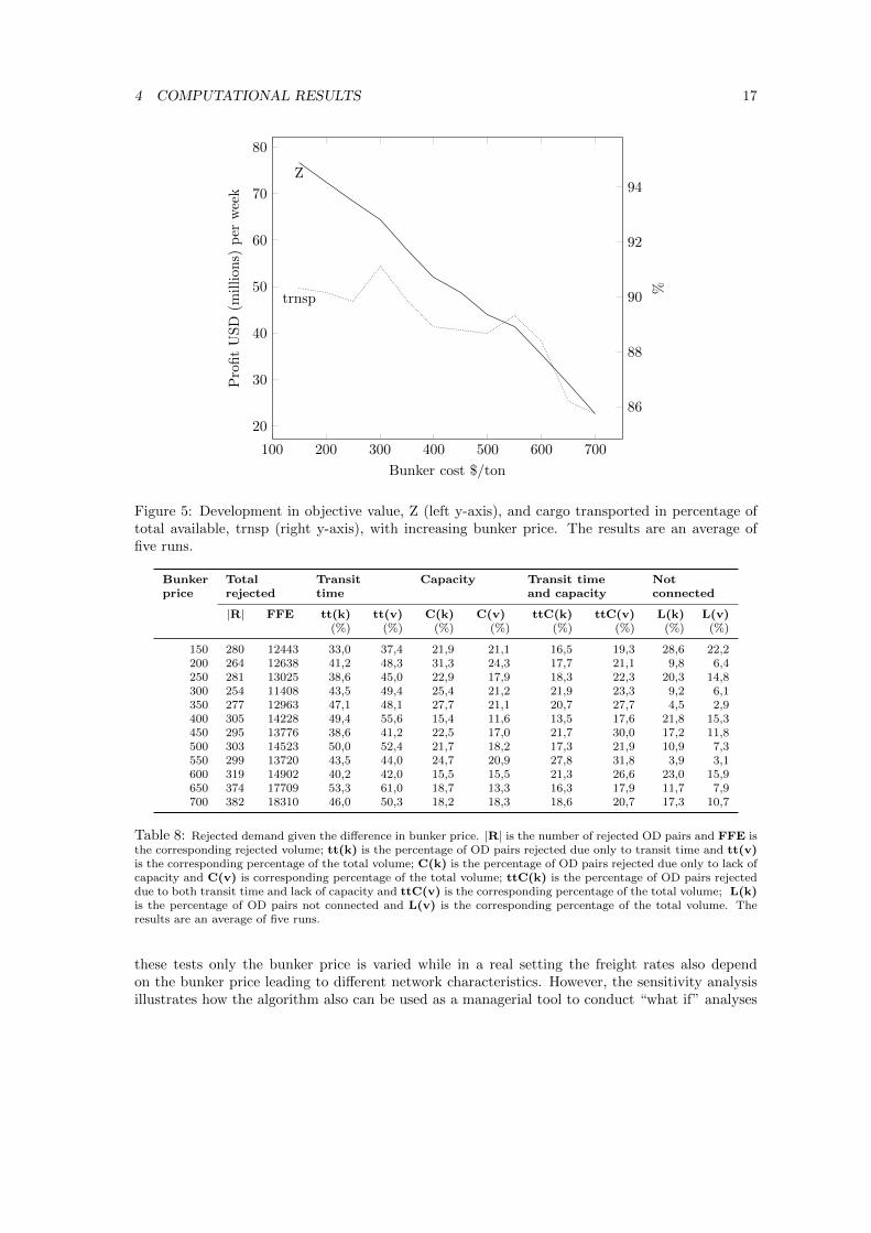
Table 7 and Figure 5 show the correlation between bunker price and the profit margin, which isdecreasing with increasing bunker prices. Furthermore, it can be seen that the amount of available


Instance Total Transit Capacity Transit time Notrejected time and capacity connected

|R| FFE tt(k) tt(v) C(k) C(v) ttC(k) ttC(v) L(k) L(v)(%) (%) (%) (%) (%) (%) (%) (%)

Baltic µ 8 732 1.1 0.2 22.6 77.1 0.0 0.0 76.3 22.7σ 1 164 3.5 0.6 11.5 10.4 0.0 0.0 14.1 10.6

WAF µ 8 712 7.0 1.2 14.0 26.1 1.7 0.1 77.3 72.6σ 2 314 12.1 2.2 9.7 25.3 5.3 0.3 13.5 24.9

Mediterranean µ 107 1527 35.3 50.0 0.2 0.4 4.3 4.0 60.1 45.7σ 8 250 7.2 9.6 0.7 1.0 4.6 3.9 5.9 8.6

Pacific µ 240 4657 51.5 34.4 7.8 27.4 13.3 29.9 27.3 8.3σ 23 641 6.7 7.4 3.3 12.6 4.1 11.8 5.9 3.4

WorldSmall µ 325 15334 35.8 40.2 19.9 16.7 21.1 23.9 23.2 19.2σ 45 1872 6.5 8.3 9.4 8.3 11.1 11.7 20.4 43.5

EuropeAsia µ 1029 11597 41.9 44.9 8.4 14.3 21.3 26.4 28.4 14.4σ 97 1008 7.5 8.3 2.9 3.5 5.8 7.3 8.5 6.3

Table 6: Statistics on the rejected demand reporting average (µ) and standard deviation (σ) over ten runs. |R|is the number of rejected OD pairs and FFE is the corresponding rejected volume; tt(k) is the percentage of ODpairs rejected due only to transit time and tt(v) is the corresponding percentage of the total volume; C(k) is thepercentage of OD pairs rejected due only to lack of capacity and C(v) is corresponding percentage of the totalvolume; ttC(k) is the percentage of OD pairs rejected due to both transit time and lack of capacity and ttC(v)is the corresponding percentage of the total volume; L(k) is the percentage of OD pairs not connected and L(v) isthe corresponding percentage of the total volume.

Bunker Obj. Val. Deployment Transp. Vol.

Price Z(7) D(v) D(|E|) T(v)($/ton) ($) (%) (%) (%)

150 7.67 · 107 91.8 95.6 90.3200 7.24 · 107 90.2 95.1 90.1250 6.85 · 107 91.0 95.3 89.8300 6.45 · 107 93.5 96.3 91.1350 5.81 · 107 94.4 95.9 89.9400 5.20 · 107 91.3 96.3 88.9450 4.86 · 107 95.0 97.3 89.3500 4.39 · 107 95.0 97.4 88.7550 4.15 · 107 94.8 96.9 89.3600 3.54 · 107 93.0 96.0 88.4650 2.90 · 107 91.5 96.2 86.2700 2.26 · 107 93.7 96.7 85.7

Table 7: Bunker price and the development in the objective value Z(7), deployment percentageof volume D(v) and number of vessels D(|E|) and the percentage of cargo transported T(v).Average of five different runs.

cargo transported only decrease a few percent with more then a quadrupling of the bunker price.In Table 9 and Figure 6 the expected trend of a decreasing speed with an increasing bunker price

is clear for all vessel classes except the SuperP class. The weighted average speed confirms thistrend. Also, Figure 6 shows how the overall deployment is increased when the speed is decreased.The algorithm performs as expected under varying conditions and confirms that even under verydifferent economics conditions we can design profitable networks. The characteristics in terms ofdeployment and sailing speed of these networks is rather different, but in all cases the algorithmis able to design networks with a high transportation percentage. It should be noted that in


100 200 300 400 500 600 700

20

30

40

50

60

70

80

Z

Bunker cost $/ton

Pro

fit

US

D(m

illi

on

s)p

erw

eek

86

88

90

92

94

trnsp

%

Figure 5: Development in objective value, Z (left y-axis), and cargo transported in percentage oftotal available, trnsp (right y-axis), with increasing bunker price. The results are an average offive runs.

Bunker Total Transit Capacity Transit time Notprice rejected time and capacity connected

|R| FFE tt(k) tt(v) C(k) C(v) ttC(k) ttC(v) L(k) L(v)(%) (%) (%) (%) (%) (%) (%) (%)

150 280 12443 33,0 37,4 21,9 21,1 16,5 19,3 28,6 22,2200 264 12638 41,2 48,3 31,3 24,3 17,7 21,1 9,8 6,4250 281 13025 38,6 45,0 22,9 17,9 18,3 22,3 20,3 14,8300 254 11408 43,5 49,4 25,4 21,2 21,9 23,3 9,2 6,1350 277 12963 47,1 48,1 27,7 21,1 20,7 27,7 4,5 2,9400 305 14228 49,4 55,6 15,4 11,6 13,5 17,6 21,8 15,3450 295 13776 38,6 41,2 22,5 17,0 21,7 30,0 17,2 11,8500 303 14523 50,0 52,4 21,7 18,2 17,3 21,9 10,9 7,3550 299 13720 43,5 44,0 24,7 20,9 27,8 31,8 3,9 3,1600 319 14902 40,2 42,0 15,5 15,5 21,3 26,6 23,0 15,9650 374 17709 53,3 61,0 18,7 13,3 16,3 17,9 11,7 7,9700 382 18310 46,0 50,3 18,2 18,3 18,6 20,7 17,3 10,7

Table 8: Rejected demand given the difference in bunker price. |R| is the number of rejected OD pairs and FFE isthe corresponding rejected volume; tt(k) is the percentage of OD pairs rejected due only to transit time and tt(v)is the corresponding percentage of the total volume; C(k) is the percentage of OD pairs rejected due only to lack ofcapacity and C(v) is corresponding percentage of the total volume; ttC(k) is the percentage of OD pairs rejecteddue to both transit time and lack of capacity and ttC(v) is the corresponding percentage of the total volume; L(k)is the percentage of OD pairs not connected and L(v) is the corresponding percentage of the total volume. Theresults are an average of five runs.

these tests only the bunker price is varied while in a real setting the freight rates also dependon the bunker price leading to different network characteristics. However, the sensitivity analysisillustrates how the algorithm also can be used as a managerial tool to conduct “what if” analyses


$/ton F450 #v F800 #v P1200 #v P2400 #v PostP #v SuperP #v Total V W. Av. S.

150 11,8 24 14,0 29 17,2 66 17,8 74 17,3 53 16,8 7 251 16,5200 11,9 24 13,5 29 17,1 67 17,8 74 17,5 50 14,0 7 250 16,5250 11,8 24 13,3 29 16,7 67 17,2 72 16,9 53 13,0 6 251 16,0300 11,9 24 13,2 28 16,6 65 17,6 74 16,8 55 18,6 7 253 16,2350 12,2 24 13,3 29 16,4 64 16,6 73 16,6 53 16,2 9 252 15,7400 11,5 24 13,7 29 16,4 68 16,7 73 16,4 55 12,4 5 253 15,7450 11,5 24 13,1 29 16,4 67 16,7 74 15,8 54 16,1 9 256 15,5500 11,7 24 13,4 29 16,2 67 16,3 74 16,1 54 15,9 8 256 15,5550 11,6 23 12,8 29 16,5 67 16,3 73 15,9 55 17,0 8 255 15,5600 11,4 24 13,4 29 16,3 67 16,5 73 15,8 52 15,3 8 252 15,4650 12,0 24 13,2 29 16,1 68 15,8 73 15,7 54 15,6 6 253 15,2700 11,7 24 13,8 29 16,1 66 15,9 74 15,3 55 15,5 7 254 15,2

Table 9: Relation between bunker price, weighted average speed per vessel class and vessel deploy-ment for each class. Weighted Average speed (W. Av. S.) is a weighted by the number of vesselsdeployed in the class (#v). The results are an average of five runs.

200 400 600

15.5

16

16.5

Bunker cost $/ton

W.A

v.S

.(n

m/h

)

200 400 600

86

88

90

Bunker cost $/ton

Trn

sp.

(%)

200 400 60095

96

97

Bunker cost $/tonD

epl.

(%)

Figure 6: The weighted average speed (W.Av.S.), of an instance, the cargo transported in per-centage of total available (Trnsp.), and the fleet capacity deployed in percentage of total volume,(Depl.) as a function of bunker price. The red dashed trend lines are based on a linear regressionfit. The results are an average of five runs.

at a strategic level.The red trend lines in Figure 6 show linear fits of the speed (f(x) = −0.002x+16.8), deployment

(f(x) = 0.002x + 95.2), and amount of transported cargo (f(x) = −0.008x + 92.2). These linearapproximations confirm the expectation that speed decrease with increased bunker price (0.2 nm/hper 100 $/ton increase), the amount transported decrease with increased bunker price (0.8 % per100 $/ton increase), and deployment increase with increased bunker price (0.2 % per 100 $/tonincrease). This is expected as the bunker consumption is cubic in speed and as the price increasewe need more vessels as the network is operating at lower speeds. This also implies that somedemands can not meet their transit times even with different service layouts.

The sensitivity analysis illustrates how the incentives towards slow steaming for liner shippingcompanies change with varying bunker prices. It will be a more active choice to maintain a greenerprofile in periods with low oil prices as attaining “an acceptable environmental performance in thetransportation supply chain, while at the same time respecting traditional economic performancecriteria” (Psaraftis, 2015) is only a win-win solution when oil prices are high.

5 CONCLUSION 19

5 Conclusion

We have presented the competitive liner shipping network design problem where we include level ofservice requirements in the form of tight transit time restrictions on all demands while maintainingthe ability to transship between services. To improve the networks, getting more realistic transittimes and a better fleet utilization, we propose a method that can handle variable speed on allsailing legs in the network.

The proposed matheuristic can handle tight transit time restrictions on all demands and adjustspeed on all sailing legs. The core components of the matheuristic is an integer program consideringa set of removals and insertions to a service and an integer program that adjust the speed ofeach service iteratively. We extend the integer program to consider how removals and insertionsinfluence the transit time of the existing cargo flow on the service. Each iteration of the matheuristicprovides a set of moves for the current set of services and fleet deployment along with a proposedsailing speed on each service leg, which lead to a potential improvement in the overall profit. Theevaluation of the cargo flow for a set of moves requires solving a time constrained multi-commodityflow problem using column generation.

Extensive computational tests, including a sensitivity analysis on bunker price, show that thealgorithm is applicable in practice and that it is possible to generate profitable networks for themajority of the instances in LINER-LIB while considering level of service requirements. Especiallyfor the larger instances the approach generates networks of good quality where the fleet is wellutilized and the majority of demands are transported while satisfying transit time restrictions.Still, some smaller demands are not served and the fleet is not utilized completely, suggesting thatfurther algorithmic improvements may lead to even better solutions. We expect that especiallymore flexibility in terms of possible vessel class swaps could improve the algorithmic performanceand the quality of the generated networks.

Acknowledgements

This project was supported by The Danish Maritime Fund under the Competitive Liner ShippingNetwork Design project. The authors would like to thank Guy Desaulniers for his contribution tothe previous works from which this article was extended and to Alessio Trivella and Niels-ChristianFink Bagger for comments which helped improving the manuscript.

A MATHEMATICAL MODEL 20

A Mathematical model

In the following we introduce a mathematical formulation of the CLSNDP. This is partly basedon Brouer et al. (2015) and extends the problem description of the LSNDP presented in Broueret al. (2014a) to handle transit times and variable speed. The model enforces a weekly frequencyresulting in a weekly planning horizon.

A solution to the CLSNDP is a subset of the set of all feasible services S. A feasible serviceconsists of a set of ports P ′ ⊆ P , a number of vessels, and a vector of sailing speeds correspondingto each sailing leg such that the total round trip time is a multiple of a week. A weekly frequencyof port calls is obtained by deploying multiple vessels to a service. Let e(s) ∈ E be the vessel classassigned to a service s and ne(s) the number of vessels of class e(s) required to maintain a weeklyfrequency. A round trip may last several weeks but due to the weekly frequency exactly one roundtrip is performed every week. The service time Ts is the time needed to complete the cyclic route.

An instance of the CLSNDP consists of the set of ports, P , with an associated port call cost cepfor vessels of class e(s), (un)load cost cpU , c

pL, transshipment cost cpT and berthing time Bp spent

on a port call. Furthermore, we have a set of demands, K, available for transport each week whereeach demand has an origin Ok ∈ P , a destination Dk ∈ P , a quantity, qk, a revenue per unit,zk, a reject penalty per unit zk and a maximal transit time, tk. To service the routes, there is aset of vessel classes, E, with specifications for the weekly charter rate, Ce, capacity Ue, minimum(vemin) and maximum (vemax) speed limits in knots per hour, bunker consumption as a function ofthe speed, gev, and bunker consumption per hour, when the vessel is idle at ports he. There are Nevessels available of class e ∈ E. The price for one metric ton of bunker is denoted cB . Finally wehave a matrix, D, of the direct distances deij between all pairs of ports i, j ∈ P and for all vesselclasses e ∈ E. The distance may depend on the vessel class draft as the Panama Canal is draftrestricted. Along with deij follows an indication of the cost leij associated with a possible traversalof a canal.

The mathematical model of the CLSNPD relies on a set of service variables and a path flowformulation of the underlying time constrained multi-commodity flow problem as described inKarsten et al. (2015a).

We define a directed graph, G(V,A), with vertices V corresponding to ports and arcs A. Theset of arcs in the graph can be divided into (un)load arcs, transshipment arcs, sailing arcs, andforfeited arcs to reject demand. We associate with each arc a ∈ A a cost ca, traversal time ta,sailing speed va, and capacity Ca. The arcs used by service s is denoted As.

Let Ωk be the set of all feasible paths for commodity k ∈ K including forfeiting the cargo. LetΩ(a) be the set of all paths using arc a ∈ A. The cost of a path ρ is denoted as cρ and it includesthe revenue obtained by transporting one unit of commodity k sent along path ρ ∈ Ωk. The realvariable xρ denotes the amount of commodity k sent along the path. The weekly cost of a service

is cs = ne(s)Ce(s) +∑

(i,j)∈As

(cB(he(s)Bp + g

e(s)v(s)d

e(s)ij ) + c

e(s)j + l

e(s)ij

)accounting for fixed cost of

deploying the vessels and the variable cost in terms of the bunker and port call cost of one roundtrip. Define binary service variables ys indicating the inclusion of service s ∈ S in the solution.

Then the mathematical model of the CLSNDP can be formulated as follows.

A MATHEMATICAL MODEL 21

min∑s∈S

csys +∑k∈K

∑ρ∈Ωk

cρxρ (23)

s.t.∑ρ∈Ωk

xρ = qk k ∈ K (24)

∑ρ∈Ω(a)

xρ ≤ Ue(s)ys s ∈ S, a ∈ As (25)

∑s∈S:e(s)=e

ne(s)ys ≤ Ne e ∈ E (26)

xρ ∈ R+ ρ ∈ Ωk, k ∈ K (27)

ys ∈ 0, 1 s ∈ S (28)

The objective (23) minimizes cumulative service and cargo transportation cost. As the cargotransportation cost includes the revenue of transporting the cargo, this is equivalent to maximizingprofit. The cargo flow constraints (24) along with non-negativity constraints (27) ensure that allcargo is either transported or forfeited. The capacity constraints (25) link the cargo paths withthe service capacity installed in the transportation network. The fleet availability constraints (26)ensure that the selected services can be operated by the available fleet. Finally, constraints (27)and (28) define the variable domains.

BIBLIOGRAPHY 22

References

Agarwal, R. and Ergun, O. (2008). Ship scheduling and network design for cargo routing in linershipping. Transportation Science, 42(2):175–196.

Alvarez, J. F. (2009). Joint routing and deployment of a fleet of container vessels. MaritimeEconomics & Logistics, 11(2):186–208.

Alvarez, J. F. (2012). Mathematical expressions for level of service optimization in liner shipping.Journal of the Operational Research Society, 63(6):709–714.

Brouer, B., Alvarez, J., Plum, C., Pisinger, D., and Sigurd, M. (2014a). A base integer program-ming model and benchmark suite for liner shipping network design. Transportation Science,48(2):281–312.

Brouer, B., Desaulniers, G., Karsten, C., and Pisinger, D. (2015). A matheuristic for the linershipping network design problem with transit time restrictions. In Corman, F., Voß, S., andNegenborn, R., editors, Computational Logistics, volume 9335 of Lecture Notes in ComputerScience, pages 195–208. Springer International Publishing.

Brouer, B., Desaulniers, G., and Pisinger, D. (2014b). A matheuristic for the liner shipping networkdesign problem. Transportation Research Part E: Logistics and Transportation Review, 72:42–59.

Cheaitou, A. and Cariou, P. (2012). Liner shipping service optimisation with reefer containers ca-pacity: an application to northern europe–south america trade. Maritime Policy & Management,39(6):589–602.

Christiansen, M. and Fagerholt, K. (2011). Some thoughts on research directions for the future:Introduction to the special issue in maritime transportation. INFOR, 49(2):75–77.

Christiansen, M., Fagerholt, K., Nygreen, B., and Ronen, D. (2013). Ship routing and schedulingin the new millennium. European Journal of Operational Research, 228(3):467–483.

Fagerholt, K., Laporte, G., and Norstad, I. (2009). Reducing fuel emissions by optimizing speedon shipping routes. The Journal of the Operational Research Society, 61(3):523–529.

Gelareh, S. and Meng, Q. (2010). A novel modeling approach for the fleet deployment problemwithin a short-term planning horizon. Transportation Research Part E: Logistics and Trans-portation Review, 46(1):76–89.

Hvattum, L. M., Norstad, I., Fagerholt, K., and Laporte, G. (2013). Analysis of an exact algorithmfor the vessel speed optimization problem. Networks, 62(2):132–135.

I. Norstad, K. F. and Laporte, G. (2011). Tramp ship routing and scheduling with speed optimiza-tion. Transportation Research Part C: Emerging Technologies, 19(5):853–865.

Karsten, C. V., Pisinger, D., Ropke, S., and Brouer, B. D. (2015a). The time constrained multi-commodity network flow problem and its application to liner shipping network design. Trans-portation Research Part E: Logistics and Transportation Review, 76:122–138.

Karsten, C. V., Ropke, S., and Pisinger, D. (2015b). Simultaneous optimization of container shipsailing speed and container routing with transit time restrictions. Technical report, TechnicalUniversity of Denmark.

Liu, Z., Meng, Q., Wang, S., and Sun, Z. (2014). Global intermodal liner shipping network design.Transportation Research Part E: Logistics and Transportation Review, 61:28–39.

REFERENCES 23

Meng, Q. and Wang, S. (2011). Optimal operating strategy for a long-haul liner service route.European Journal of Operational Research, 215(1):105–114.

Meng, Q., Wang, S., Andersson, H., and Thun, K. (2014). Containership routing and scheduling inliner shipping: Overview and future research directions. Transportation Science, 48(2):265–280.

Notteboom, T. E. and Vernimmen, B. (2009). The effect of high fuel costs on liner service config-uration in container shipping. Journal of Transport Geography, 17(5):325–337.

Plum, C., Pisinger, D., and Sigurd, M. M. (2014). A service flow model for the liner shippingnetwork design problem. European Journal of Operational Research, 235(2):378–386.

Psaraftis, H. N. (2015). Green Transportation Logistics: The Quest for Win-Win Solutions, volume226. Springer.

Psaraftis, H. N. and Kontovas, C. A. (2013). Speed models for energy-efficient maritime trans-portation: A taxonomy and survey. Transportation Research Part C: Emerging Technologies,26:331–351.

Reinhardt, L. B. and Pisinger, D. (2012). A branch and cut algorithm for the container shippingnetwork design problem. Flexible Services and Manufacturing Journal, 24(3):349–374.

Reinhardt, L. B., Pisinger, D., Plum, C. E., Sigurd, M. M., and Vial, G. T. (2015). The linershipping berth scheduling problem with transit times. Transportation Research Part E: Logisticsand Transportation Review, page submitted.

Ronen, D. (2011). The effect of oil price on containership speed and fleet size. Journal of theOperational Research Society, 62(1):211–216.

Wang, S. and Meng, Q. (2012a). Liner ship fleet deployment with container transshipment opera-tions. Transportation Research Part E: Logistics and Transportation Review, 48(2):470–484.

Wang, S. and Meng, Q. (2012b). Liner ship route schedule design with sea contingency time andport time uncertainty. Transportation Research Part B: Methodological, 46(5):615–633.

Wang, S. and Meng, Q. (2012c). Sailing speed optimization for container ships in a liner shippingnetwork. Transportation Research Part E: Logistics and Transportation Review, 48(3):701–714.

Wang, S. and Meng, Q. (2014). Liner shipping network design with deadlines. Computers andOperations Research, 41(1):140–149.

Zacharioudakis, P. G., Iordanis, S., Lyridis, D. V., and Psaraftis, H. N. (2011). Liner shippingcycle cost modelling, fleet deployment optimization and what-if analysis. Maritime Economics& Logistics, 13(3):278–297.

DTU Management Engineering Institut for Systemer, Produktion og Ledelse Danmarks Tekniske Universitet Produktionstorvet Bygning 424 2800 Kongens Lyngby Tlf. 45 25 48 00 Fax 45 93 34 35 www.man.dtu.dk

We present a solution method for the liner shipping network design problem which is a core strategic planning problem faced by container carriers. We propose the first practical algorithm which explicitly handles transshipment time limits for all demands. Individual sailing speeds at each service leg are used to balance sailings speed against operational costs, hence ensuring that the found network is competitive on both transit time and cost. We present a matheuristic for the problem where a MIP is used to select which ports should be inserted or removed on a route. Computational results are presented showing very promising results for realistic global liner shipping networks. Due to a number of algorithmic enhancements, the obtained solutions can be found within the same time frame as used by previous algorithms not handling time constraints. Furthermore we present a sensitivity analysis on fluctuations in bunker price which confirms the applicability of the algorithm

Competitive Liner Shipping Network Design · The paper by Agarwal and Ergun (2008) imposes a weekly...

Documents

Transcript of Competitive Liner Shipping Network Design · The paper by Agarwal and Ergun (2008) imposes a weekly...