Competing with Asking Prices∗

Benjamin Lester†

Federal Reserve Bank of Philadelphia

Ludo Visschers‡

University of Edinburgh

& Universidad Carlos III, Madrid

Ronald Wolthoff

University of Toronto

October 24, 2013

Abstract

In many markets, sellers advertise their good with an asking price. This is a price at which

the seller will take his good off the market and trade immediately, though it is understood that

a buyer can submit an offer below the asking price and that this offer may be accepted if the

seller receives no better offers. Despite their prevalence in a variety of real world markets,

asking prices have received little attention in the academic literature. We construct an envi-

ronment with a few simple, realistic ingredients and demonstrate that using an asking price is

optimal: it is the pricing mechanism that maximizes sellers’ revenues and it implements the

efficient outcome in equilibrium. We provide a complete characterization of this equilibrium

and use it to explore the positive implications of this pricing mechanism for transaction prices

and allocations.

Keywords: Asking Prices, Directed Search, Inspection Costs, Efficiency

JEL codes: C78, D44, D82, D83, L11, R31, R32

∗We would like to thank Jim Albrecht, Jan Eeckhout, Andrea Galeotti, Pieter Gautier, Lu Han, Benoit Julien,Philipp Kircher, Guido Menzio, Peter Norman, Jozsef Sakovics, Shouyong Shi, Andy Skrzypacz, Xianwen Shi, RobShimer, Susan Vroman, Gabor Virag, and Randy Wright for helpful comments. All errors are our own.†The views expressed here are those of the authors and do not necessarily reflect the views of the Fed-

eral Reserve Bank of Philadelphia or the Federal Reserve System. This paper is available free of charge atwww.philadelphiafed.org/research-and-data/publications/working-papers/.‡Ludo Visschers gratefully acknowledges financial support from the Juan de la Cierva Grant; project grant

ECO2010-20614 (Direccion general de investigacion cientıfica y tecnica), and the Bank of Spain’s Programa de In-vestigacion de Excelencia.

1

“We are eager to hear ... about businesses that meet all of the following criteria:

(1) Large purchases; (2) Demonstrated consistent earning power; (3) Businesses earning good

returns on equity while employing little or no debt; (4) Management in place; (5) Simple

businesses; (6) An offering price (we don’t want to waste our time or that of the sellerby talking, even preliminarily, about a transaction when price is unknown)... We don’tparticipate in auctions.”1

– Berkshire Hathaway Inc., “Acquisition Criteria,” 2012 Annual Report

1 Introduction

In this paper, we consider an environment in which a trading mechanism that we call an asking

price emerges as an optimal way of coping with certain frictions. In words, an asking price isa price at which a seller commits to taking his good off the market and trading immediately.However, it is understood that a buyer can submit an offer below the asking price and such anoffer could potentially be accepted if the seller receives no better offers.2 Though asking pricesare prevalent in a variety of real world markets, they have received relatively little attention inthe academic literature. We construct an environment with a few simple, realistic ingredients anddemonstrate that using an asking price is both revenue-maximizing and efficient; that is, sellersoptimally choose to use the asking price mechanism and, in equilibrium, the asking prices theyselect implement the solution to the planner’s problem. We provide a complete characterizationof this equilibrium and use it to explore the positive implications of this pricing mechanism fortransaction prices and allocations.

At first glance, one might think that committing to an asking price would be sub-optimal froma seller’s point of view. After all, the seller is not only placing an upper bound on the price thata buyer might propose, he is also committing not to meet with any additional prospective buyersonce the asking price has been offered. Hence, when a buyer purchases the good at the askingprice, the seller has forfeited any additional rents that either this buyer or other prospective buyerswere willing to pay. And yet, anybody who has recently purchased a house or a car, rented anapartment, walked through a bazaar, or perused the classifieds knows that an asking price seems toplay a prominent role in the sale of many goods (and services). The question is: how and why canthis mechanism be optimal?

1Bold added for emphasis; italics present in original.2What we call an asking price goes by several other names as well, including an “offering price” (as in the epi-

graph), a “list price” (used in the sale of houses and cars), or a “buy-it-now” or “take-it” price (used in certain onlinemarketplaces). In many classified advertisements, what we call an asking price often comes in the form of a pricefollowed by the comment “or best offer.” Though the terminology may differ across these various markets, alongwith the fine details of how trade occurs, we think our analysis identifies an important, fundamental reason that sellersmight find this basic type of pricing mechanism optimal.

2

Loosely speaking, our answer requires two ingredients. First, the sellers in our environmentcompete for buyers. That is, in contrast to the large literature that studies the performance of varioustrading mechanisms (e.g., auctions) when the number of buyers is fixed, we assume that there aremany sellers, each one posts (and commits to) the process by which their good will be sold, andbuyers strategically choose to visit only those sellers who promise the maximum expected payoff.Thus, in our framework, the number of buyers at each seller is responsive to the mechanism theypost. The second ingredient is that the goods for sale are inspection goods and inspection is costly:though all sellers’ goods appear ex ante identical, in fact each buyer has an idiosyncratic (private)valuation for each good which can only be learned through a process of costly inspection.3

In an environment with these two ingredients, a natural tension arises. Ceteris paribus, sellerswould like to place no limit on the number of buyers who inspect their good or on the offers thatthese buyers make. However, such a pricing mechanism is not particularly attractive to buyers.Instead, when a buyer incurs the inspection cost, he wants to be assured that he has a reasonablechance of actually acquiring the good (i.e., that another buyer hasn’t already inspected the goodand discovered a very high valuation). We show that the asking price mechanism provides thisassurance by implementing a stopping rule, so that the good is allocated to the first buyer whohas a sufficiently high valuation, and spares the remaining potential buyers from inspecting thegood “in vain.” In other words, echoing the sentiments of Berkshire Hathaway’s chairman WarrenBuffett in the epigraph above, the asking price mechanism in our model serves as a promise by

sellers not to waste the buyers’ time and energy. In a competitive setting, this promise is themost effective way for a seller to attract buyers and thus, in equilibrium, sellers use this pricingmechanism. Moreover, the asking price that sellers choose ultimately maximizes the expectedsurplus that they create, so that equilibrium asking prices implement the planner’s solution.

Having provided the rough intuition, we now discuss our environment and main results ingreater detail. As we describe explicitly in Section 2, we consider a market with a measure ofsellers, each endowed with one indivisible good, and a measure of buyers who each have unitdemand. Though goods appear ex ante identical, each buyer has an idiosyncratic valuation foreach good and this valuation can only be learned through a costly inspection process. We assumethat sellers have the ability to communicate ex ante (or “post”) how their good is going to be sold,

3For example, suppose the goods are houses that are roughly equivalent along easily describable dimensions (size,general location, and so on). However, each home has idiosyncratic features that may make them more or less attractiveto every prospective buyer, and these features are revealed upon inspection; e.g., an individual who likes to cook willwant to examine a home’s kitchen. Quite often, learning one’s true valuation may require more research than isafforded by a quick tour; e.g., an individual who needs to build a home office may want to bring in an architect toget an estimate of how much it will cost. All of these activities are costly, either because they take time or becausethey require explicit costs (like hiring an architect). Similar costs exist for purchasing a car, renting an apartment, oreven hiring an accountant. Perhaps surprisingly, these costs can even be significant for buyers purchasing goods onwebsites such as eBay or Craigslist, as documented by Bajari and Hortacsu (2003).

3

and buyers can observe what each seller posts and visit the seller that offers the highest expectedpayoff. The matching process, however, is frictional: each buyer can only visit a single seller andhe cannot coordinate this decision with other buyers. As a result, the number of buyers to arrive ateach seller is a random variable with a distribution that depends on what the seller posted.

As a first step, in Section 3 we characterize the solution to the problem of a social planner whomaximizes total surplus, subject to the frictions described above — in particular, the matchingfrictions and the requirement that a buyer’s valuation is costly to learn. The solution has threeproperties. First, the planner instructs buyers to randomize evenly across sellers. Second, once arandom number of buyers arrive at each seller, the planner instructs buyers to undergo the costlyinspection process sequentially, preserving the option to stop after each inspection and allocate thegood to one of the buyers who have learned their valuation. This strategy of “sequential searchwith recall” is optimal because it balances the losses associated with additional buyers incurringthe inspection cost against the gains associated with finding a buyer who values the good morethan all of the previous buyers. Finally, we characterize the optimal stopping rule for this strategyand establish that it is stationary; that is, it depends on neither the number of buyers who haveinspected the good nor the realization of their valuations.

Next, we move on to our main contribution: we consider the decentralized economy, character-ize the trading mechanism that emerges in equilibrium, and study the efficiency properties of thisequilibrium. Given the nature of the planner’s optimal trading protocol, the asking price mech-anism is a natural candidate to implement the efficient outcome. First, since buyers’ valuationsare privately observed, the asking price provides sellers a channel to elicit information about thesevaluations. Second, since the asking price triggers immediate trade, it implements a stopping rule,thus preventing additional buyers from incurring the inspection cost when the current buyer drawsa sufficiently high valuation. Finally, since the seller also allows bids below the asking price, heretains the option to recall previous offers in which there was a positive match surplus.

These features are captured by the following game, which we study in Section 4. First, sellerspost an asking price, which all buyers observe. Given these asking prices, each buyer then choosesto visit the seller (or mix between sellers) offering the maximal expected payoff. Once buyers arriveat their chosen seller, they are placed in a random order. Buyers are told neither the number of otherbuyers who have arrived, nor their place in the queue.4 The first buyer incurs the inspection cost,learns his valuation, and can either purchase the good immediately at the asking price or submita counteroffer. If he chooses the former, trade occurs and all remaining buyers at that particularseller neither inspect the good nor consume. If he chooses the latter, the seller moves on to thesecond buyer (if there is one) and the process repeats until either the asking price is offered or the

4As we discuss below, we consider the information made available to buyers to be a feature of the pricing mecha-nism.

4

queue of buyers is exhausted, in which case the seller can accept the highest offer he has received.We derive the optimal bidding behavior of buyers and the optimal asking prices set by sellers,

characterize the equilibrium, and show that it coincides with the solution to the planner’s problem.The fact that such a simple, realistic instrument as our asking price mechanism can implement theefficient allocation is surprising for a number of reasons, as we discuss at the end of Section 4.Chief among them, implementing the planner’s allocation requires achieving efficiency along two

margins: the allocation of the good after buyers arrive, along with the number of buyers that arriveto begin with. However our asking price mechanism affords sellers only a single price — withoutany other devices such as meeting fees, bidding subsidies, or reserve prices — that controls bothmargins; it determines the ex-post allocation of the good (by implementing a stopping rule) andthe ex-ante expected number of buyers (by specifying the division of the expected surplus).

After establishing that the asking price mechanism implements the solution to the plannersproblem, we ask whether sellers would indeed choose to use the asking price mechanism, or ifthere exists an alternative mechanism that could potentially increase sellers’ profits. To addressthis question, in Section 5 we consider a similar game to the one described above, but we allowsellers to select a mechanism from an arbitrary set of pricing schemes. In this more general envi-ronment, we establish that an asking price mechanism maximizes a seller’s payoff, irrespective ofthe mechanisms posted by other sellers. As a consequence, there always exists an equilibrium inwhich all sellers use the asking price mechanism described above. Moreover, while other equilibriacan exist, they are all payoff-equivalent; in particular, there is no equilibrium in which sellers earnhigher expected payoffs than they do in the equilibrium with asking prices. Finally, we show thatany mechanism that emerges as an equilibrium in this environment will resemble the asking pricemechanism along most important dimensions. Therefore, though we cannot rule out potentiallycomplicated mechanisms that also satisfy the equilibrium conditions, the fact that asking pricesare both simple and commonly observed suggests that they are a robust and compelling way todeal with the frictions in our environment.

The normative analysis described above leaves us with a tractable, micro-founded theory ofasking prices, which we think could be a useful benchmark for both theoretical and empirical workthat focuses on markets in which this pricing mechanism is prevalent. In Section 6, we flesh outjust a few of the model’s positive implications for a variety of observable outcomes. In particular,we study the level of asking prices set by sellers and the corresponding distribution of transactionprices that occur in equilibrium. We examine how these variables change with features of theenvironment, such as the ratio of buyers to sellers, the degree of ex ante uncertainty in buyers’valuations, and the costs of inspecting the good. Moreover, we analyze the relationship betweenthe expected transaction price and the number of buyers who inspect the good before trade; tothe extent that each inspection takes time, this analysis provides new insights into the relationship

5

between transaction prices and time on the market.In Section 7, we discuss a few of our key assumptions, along with several interesting extensions

of our basic framework. A number of these extensions could be particularly helpful for taking ourmodel to data. For one, we show that a simple variation of our asking price mechanism wouldproduce a distribution of transaction prices that occur below the asking price, a mass point oftransactions that occur at the asking price, and additional transactions that occur above the asking

price. This variation, which preserves all of the normative properties reported above, could be animportant step towards confronting, e.g., house prices.5 We also discuss how allowing for hetero-geneity across buyers could lead to endogenous market segmentation, where each sub-market hasa different asking price, a different market tightness, and subsequently produces different patternsfor prices and allocations. Finally, section 8 concludes and the Appendix contains all proofs.

Related Literature. We contribute to the literature along two dimensions. The first is norma-tive: we show that an uncomplicated, realistic instrument — the asking price — is both revenue-maximizing and efficient in an environment with two simple ingredients. The second is positive:we provide a rationale for the use of asking prices — namely, as a promise by sellers not to wastebuyers’ time and resources — and explore the empirical implications of this mechanism for equi-librium prices and allocations. Below, we compare our normative and positive results, respectively,with the existing literature.

As mentioned above, implementing the planner’s allocation requires achieving efficiency alongtwo margins. First, a seller’s mechanism has to induce socially efficient search behavior by buyers;this requires that each buyer’s ex ante expected payoff is equal to his marginal contribution to theexpected surplus at that seller. Second, a seller’s mechanism must maximize the surplus after arandom number of buyers arrive; that is, the mechanism must ensure that the ex post allocation ofthe good is efficient. These two margins have been studied extensively in separate literatures.

The first margin is a critical object of interest in the literature on competitive (or directed)search, such as Moen (1997), Burdett et al. (2001), Acemoglu and Shimer (1999), and Julienet al. (2000), to name a few. While these papers have often found that the market equilibriumdecentralizes the planner’s solution, their results do not extend to our environment. The reasonis that, in these papers, the size of the surplus after buyers arrive is independent of the pricingmechanism. Hence, a simple mechanism, like a price or a wage, can control the division of theexpected surplus in an arbitrarily flexible way without any ramifications for ex post efficiency.Therefore, within this literature, the papers that are most related to our work are McAfee (1993),

5Case and Shiller (2003) and Han and Strange (2013) document housing prices and show that a significant fractionof transactions occur at the asking price, and (in some locations) a number of transactions also occur above the askingprice.

6

Peters and Severinov (1997), Burguet and Sakovics (1999), Eeckhout and Kircher (2010), Virag(2010), Kim and Kircher (2012), and Albrecht et al. (2012b), who consider environments where thepricing mechanism that is posted does effect the size of the surplus after buyers arrive. However,in these papers the ex post efficient allocation of the good is typically fairly trivial, and hence canbe implemented with a simple, simultaneous mechanism (like an auction with no reserve price).

In contrast, our model — where buyers incur a cost to learn their valuation — requires that weconsider a competitive search model where sellers post sequential mechanisms. We establish thatthe mechanism that achieves the efficient ex post allocation also induces efficient search decisionsby buyers ex ante. Moreover, this sequential mechanism is surprisingly simple: it does not requirethat sellers have access to rarely observed devices like meeting fees or bidding subsidies, whichallow sellers to transfer or appropriate part of the expected surplus without affecting its size.

Sequential mechanisms have received much more attention in the literature that focuses onthe second margin highlighted above but abstracts from the first margin, i.e., the literature thatstudies the allocation of a good when a monopolist seller faces a fixed number of buyers who canlearn their valuation at a cost. However, the prevailing wisdom in this literature is that the optimalmechanism in this environment will require that the seller have access to a number of differentinstruments. For example, Cremer et al. (2009) show that, in this type of environment, the selleroptimally selects a sequential mechanism that requires a series of different take-it-or-leave-it offersand participation fees, both of which may vary according to the number and realizations of previousbids.6 Deeming such a mechanism implausibly elaborate and demanding, Bulow and Klemperer(2009) instead focus on two “plain vanilla” mechanisms — a simultaneous auction and a simplesequential mechanism — and identify a trade-off between revenue-maximization and efficiency.In contrast to these papers, the mechanism we consider is remarkably simple (sellers post a singlenumber) and yet the trade-off in Bulow and Klemperer (2009) does not arise; the asking price isboth revenue-maximizing and efficient.7

The reason our results differ from those in the existing literature is twofold. The first crucialdifference is that the number of buyers who can potentially inspect a seller’s good is exogenousin the papers cited above, whereas in our model it is endogenous. Hence, the sellers in our modelhave an incentive to post mechanisms that implement the efficient allocation, since they are the

6These take-it-or-leave-it offers act like a sequence of asking prices which, along with participation fees, arecalibrated just right to extract all of the buyers’ surplus. In a similar environment, Burguet (1996) also shows that oneway to implement the efficient allocation is through a relatively complicated sequence of reserve prices and biddingsubsidies.

7Roberts and Sweeting (2012) also compare the performance of a simultaneous auction and a simple sequentialmechanism, though they assume buyers have some information about their valuation before making an entry decision.Interestingly, the asking price mechanism in our model convexifies, in a way, the binary choice between these twopricing schemes; as we discuss below, one can interpret our mechanism in such a way that the asking price determinesthe probability of having an auction (after all buyers have inspected the good) as opposed to a sequential sale.

7

residual claimant on any extra surplus that they create.8 The second crucial difference betweenour environment and that of, e.g., Cremer et al. (2009) and Bulow and Klemperer (2009) is thatthese papers assume that prospective buyers observe both the number and behavior of previousbidders who have entered the mechanism, whereas we allow the sellers in our model to choosewhat information is available. Importantly, they choose not to reveal information about previousbidders. Instead, when the buyers in our model inspect the good, they only know that no previousbidder has discovered a valuation high enough to bid the asking price. As we discuss in greaterdetail in Section 4, this (endogenously determined) information structure is one important reasonthat the trade-off in Bulow and Klemperer (2009) disappears in our environment.

Turning to the positive results, our explanation is of course not the only plausible reason whyasking prices might serve a useful role. For one, if buyers are risk averse, an asking price offers away of reducing the uncertainty an individual buyer faces in certain (not necessarily optimal) typesof auctions, and hence introducing this mechanism can potentially increase a seller’s revenues;see, e.g., Budish and Takeyama (2001), Mathews (2004), or Reynolds and Wooders (2009). Asecond explanation for asking prices, which also assumes that it is costly for buyers to learn theirvaluation, is proposed by Chen and Rosenthal (1996) and Arnold (1999). In their environment, aholdup problem emerges when a buyer and seller bargain over the terms of trade after the buyerincurs the inspection cost. An asking price is treated as a ceiling on the bargaining outcome andthus partially solves this holdup problem. This explanation is close to ours in spirit, in the sensethat an asking price serves as an ex ante guarantee that some rents will be transferred from the sellerto the buyer. However, in contrast to our work, the asking price in these papers has no allocativerole, nor is it clear that the asking price is the most efficient way of solving this holdup problem.9

A trading mechanism that bears some resemblance to an asking price can also emerge if itis costly for sellers to meet with each buyer, as in McAfee and McMillan (1988). In this case,the price that sellers advertise serves as a commitment device to keep meeting with buyers untila sufficiently high bid has been received, despite an incentive ex post to stop earlier. Hence,this quoted price is playing the opposite role as the asking price in our model; according to ourexplanation, asking prices serve as a promise to stop sampling after a sufficiently high bid, despite

8This insight is not only true in the competitive search models cited above, but also in a very related literaturethat studies a single seller who selects the mechanism by which they want to sell their good, and a number of buyerswho can choose to participate in the mechanism; see Engelbrecht-Wiggans (1987), McAfee and McMillan (1987), andLevin and Smith (1994) for seminal contributions. The difference is that the “cost” to a buyer from visiting a seller inthe former literature is the opportunity cost of not visiting other sellers (which is an equilibrium object), while the costof participating in the latter is an explicit entry cost (which is taken as exogenous).

9More generally, these theories of asking prices consider the problem of a seller in isolation. Therefore, thougheach one certainly captures a significant component of what asking prices do, they also abstract from somethingimportant: the fact that buyers can observe and compare multiple asking prices at once is not only realistic in manymarkets, but also seems to be a principal consideration when sellers are determining their optimal pricing strategy.

8

an incentive ex post to continue.10

Finally, asking prices may serve as a device to signal sellers’ private information. For exam-ple, in Albrecht et al. (2012a), sellers with heterogeneous reservation values use asking prices tosignal their type, which allows for endogenous market segmentation. We view this line of researchas complementary to our own; certainly the ability of asking prices to signal a seller’s privateinformation, which we ignore, is important.11

2 The Environment

Players. There is a measure θb of buyers and a measure θs of sellers, so that Λ = θb/θs denotes theratio of buyers to sellers. Buyers each have unit demand for a consumption good, and sellers eachpossess one, indivisible unit of this good. All agents are risk-neutral and ex ante homogeneous.

Matching. Buyers can visit a single seller in attempt to trade, but the matching process is fric-tional. In particular, buyers cannot coordinate with one another when choosing a seller to visit,and hence the number of buyers to arrive at each seller, n, will be stochastic. As is customary inthe literature on directed (or competitive) search, we assume that n is distributed according to thePoisson distribution with parameter λ, which represents the expected number or “queue length” ofbuyers to arrive at a particular seller.12 As we describe in detail below, the queue length at eachseller will be an endogenous variable, determined by the equilibrium behavior of buyers and sellers.

Preferences. All sellers derive utility y from consuming their own good, and this valuation iscommon knowledge. A buyer’s valuation for any particular good, on the other hand, is not knownex ante. Rather, once buyers arrive at a particular seller, they must inspect the seller’s good inorder to learn their valuation, which we denote by x. We assume that each buyer’s valuation isan iid draw from a distribution F (x) with continuous support on the interval [x, x], and that therealization of x is the buyer’s private information.

10To be more precise, McAfee and McMillan (1988) consider a procurement auction in which a buyer meets witha sequence of sellers and each meeting is costly to the buyer; this is equivalent to our environment with the sellerincurring the cost of each meeting. Switching which party bears the inspection cost not only changes the entirerationale for an asking price, as described above, but it also changes the nature of the revenue-maximizing mechanism;the solution to our model with this alternative cost structure is available upon request.

11Menzio (2007), Delacroix and Shi (2013) and Kim and Kircher (2012) also study the signalling role of prices indirected search equilibria. However, in papers like Albrecht et al. (2012a) and Menzio (2007), asking prices are notuniquely determined, and hence these models are somewhat limited in their ability to draw positive implications aboutthe relationship between asking prices, transaction prices, and market conditions.

12The Poisson distribution is commonly used in these models because there are explicit micro-foundations: one canstudy a game with a finite number of agents in which each buyer chooses a single seller, but buyers are restricted tosymmetric strategies. The matching technology that emerges—urn-ball matching—converges to a Poisson matchingfunction as the number of buyers and sellers gets large. See, e.g., Burdett et al. (2001).

9

We assume, for simplicity, that y ∈ [x, x] . This is a fairly weak assumption; the probabilitythat a buyer’s valuation x is smaller than y can be driven to zero without any loss of generality.However, we stress that much of the analysis remains similar when y < x, though the algebra isslightly more involved.

Inspection Costs. A key friction in the model is that the process of inspecting a good is costlyto the buyer. In particular, after a buyer arrives at a seller, we assume that he must pay a cost kin order to learn his valuation x. Such costs come in many forms. For instance, when a buyer islooking to purchase a car, it is costly for him to take time away from other productive activities tosit down with the seller, go over the car, take it for a test drive, and perhaps take it to a mechanicto be inspected. We use k to capture all of these costs, both implicit and explicit.

We restrict our attention to the region of the parameter space in which the cost of inspectingthe good does not exhaust the expected gains from trade. In particular, we assume that

k <

∫ x

y

(x− y) f(x)dx. (1)

Note that the inequality in (1) does not necessarily imply that a buyer would always choose toinspect the good. In what follows, we will assume that a buyer indeed does have incentive to in-spect the good before attempting to purchase it, and in Section 7 we derive a sufficient conditionto ensure that this is true in equilibrium.

Gains from Trade. When n buyers arrive at a seller, the trading protocol in place will determinehow many buyers i ≤ nwill have the opportunity to inspect the good before exchange (potentially)occurs. We normalize the payoff for a buyer who does not inspect, and thus does not trade, to zero.Therefore, if a buyer with valuation x acquires the good after the seller has met with i buyers, thenet social surplus from trade is x− y − ik. Alternatively, if the seller retains the good for himselfafter i inspections, the net social surplus is simply −ik.

3 The Planner’s Problem

In this section, we will characterize the decision rule of a (constrained) benevolent planner whoseobjective is to maximize net social surplus, subject to the constraints of the physical environment.These constraints include the frictions inherent in the matching process, as well as the requirementthat buyers’ valuations are costly to learn.

The planner’s problem can be broken down into two components. First, the planner has toassign queue lengths of buyers to each seller, subject to the constraint that the sum of these queue

10

lengths across all sellers cannot exceed the total measure of available buyers, θb. Second, the plan-ner has to specify the trading rules for agents to follow after the number of buyers that arrive at eachseller is realized. Working backward, we begin by characterizing these trading rules at an arbitraryseller, taking the queue length as given, and return later to characterize the optimal assignment ofqueue lengths across sellers.

Optimal Trading Protocol. Suppose n buyers arrive at a seller. The first result that we presentin this section is that it is optimal for the planner to learn the buyers’ valuations sequentially (i.e.,one at a time), preserving the option to stop after each inspection i ≤ n and allocate the good toeither one of the i buyers who has inspected the good, or to instruct the seller to retain the goodfor himself. Intuitively, this sequential search strategy is optimal because it allows the decision ofwhether an additional buyer should incur the inspection cost to be contingent on the realization ofprevious buyers’ valuations; the planner can economize on k if the expected gain from learning thevaluation of one or more additional buyers is small. The proof of this result is straightforward andfollows very closely to that in Morgan and Manning (1985).

Lemma 1. The optimal strategy for the planner is a sequential search strategy.

We now characterize the planner’s optimal stopping rule. In general, after a seller has met withi buyers with valuations (x1, ..., xi), when n ≥ i total buyers have arrived, the planner’s decisionrule is a function that dictates whether a seller should (a) keep meeting with additional buyers (ifthere are any), (b) trade with buyer i′ ∈ {1, ..., i}, or (c) retain the good for his own consumption.However, several features of the environment simplify this function immediately. First, notice thatthe only relevant information in the vector (x1, ..., xi) is the maximum valuation; clearly, if theplanner instructs the seller to stop meeting buyers, the good must be allocated to either the buyerwith the highest valuation or the seller himself. Given this, it will be convenient to denote byxi ≡ max{y, x1, ..., xi}. Second, while the cost of an additional meeting between the seller anda buyer is a constant (k), we conjecture and later confirm that the continuation value of meetingwith the (i + 1)th buyer is increasing in xi, so that the planner’s optimal decision rule is a cutoffstrategy. Let us denote the planner’s cutoff by xpi,n for n ∈ N\{1} and i ∈ {1, 2, ..., n− 1}, so thatthe seller will stop meeting buyers and the good will be consumed by the agent with valuation xi if,and only if, xi ≥ xpi,n. Otherwise, if xi < xpi,n, the seller will continue to meet with the next buyer.Below we establish that, in fact, the optimal stopping rule is stationary; in particular, it does notdepend on the number of buyers who have already inspected the good, i, or the number of buyersstill available to inspect the good, n− i.13

13See Lippman and McCall (1976) for a similar result. It is worth noting that the stationarity of xpi,n implies thatwhether or not the planner can observe i and/or n is ultimately immaterial, as he would choose the same cutoff rule ineither environment.

11

Lemma 2. Suppose n ∈ N buyers arrive at a seller. Letting x∗ satisfy

k =

∫ x

x∗(x− x∗)f(x)dx, (2)

the planner maximizes the social surplus implementing the following rule:

(i) If n > 1 and i ∈ {1, 2, ..., n − 1}, the seller should stop meeting with buyers and allocate

the good to the agent with valuation xi if, and only if, xi ≥ xpi,n = x∗. Otherwise, the seller

should meet with the next buyer.

(ii) If n=1 or i = n, the seller should allocate the good to the agent with valuation xn.

The proof of Lemma 2 utilizes an induction argument; we sketch the first step here, for intu-ition, and present the formal proof in the appendix. Suppose an arbitrary number n ≥ 2 buyersarrive at a seller, and let Zn−j,n(x) − y denote the net expected surplus from continuing to learnbuyers’ valuations, given that the maximum valuation of the seller and the n − j buyers sampledso far is x, for some j ∈ {1, 2, ..., n − 1}. For notational convenience, we will drop the secondsubscript “n”, so that Zn−j,n(x) ≡ Zn−j(x), xpn−j,n ≡ xpn−j , and so on; it should be understoodthat the analysis is for an arbitrary value of n.

Figure 1 plots Zn−1(x), Zn−2(x), and x. Notice three facts: (i) Zn−1(x) > x if and only ifx < x∗; (ii) Zn−2(x) > Zn−1(x) if and only if x < x∗; and (iii) Zn−2(x) = Zn−1(x) for x ≥ x∗.The first of these facts is by construction: x∗ is defined as the value of x that makes the plannerindifferent between learning the valuation of one additional buyer and stopping. Hence, it is shouldbe obvious that xpn−1 = x∗ is optimal.

INSERT FIGURE 1 HERE

Now consider the second and third facts. Intuitively, Zn−2(x) − Zn−1(x) ≥ 0 captures theoption value of being able to sample two more buyers instead of only one. However, if xn−2 ≥x∗ = xpn−1, then this option is never exercised after n − 1 valuations have been discovered, andthus Zn−2(x) = Zn−1(x); since the nth buyer is never sampled, both Zn−2(x) and Zn−1(x) denotethe expected surplus from sampling just one more buyer. Alternatively, if xn−2 < x∗ = xpn−1,then the option to sample two more buyers instead of one can be valuable, but this additional valueis realized only in the event that xn−1 ∈ (xn−2, x

∗): if xn−1 < xn−2 then xn−2 = xn−1, and ifxn−1 > x∗ then the nth buyer is never sampled. Hence, as xn−2 → x∗, this option value convergesto zero and Zn−2(x) → Zn−1(x). As a result, clearly Zn−2(x) > x if and only if x < x∗; that is,xpn−2 = x∗ is optimal. This completes the sketch of the first induction step; the remainder proceedsin much the same way.

12

Optimal Queue Lengths. We turn now to the optimal assignment of queue lengths across sellers,given the planner’s decision rule for after buyers arrive. Notice immediately that the planner’soptimal cutoff is not only independent of n and i, it is also independent of λ, which governs thedistribution over n. The reason is that the optimal stopping rule, on the margin, balances the costsand expected gains of additional meetings, conditional on the event that there are more buyersin the queue. The probability of this event, per se, is irrelevant: since the seller neither incursadditional costs nor forfeits the right to accept any previous offers if there are no more buyers inthe queue, the probability distribution over the number of buyers remaining in the queue — andthus λ — does not affect the planner’s choice of xp.

Let S (xp, λ) denote the expected surplus generated at an individual seller who is assigned acutoff xp and a queue length λ. In order to derive this function, it will be convenient to define

qi(x;λ) =λi (1− F (x))i

i!e−λ(1−F (x)). (3)

In words, qi(x;λ) is the probability that a seller is visited by exactly i buyers who draw a valuationgreater than x (when all buyers’ valuations are learned). In what follows, we will suppress theargument λ for notational convenience.

The net surplus generated at a particular seller is equal to the gains from trade, less the inspec-tion costs. To derive the expected gains from trade at a seller with cutoff xp and queue length λ,first suppose that n buyers arrive at this seller. There are three relevant cases. First, with probabilityF (y)n all n buyers draw valuation x < y, in which case there are no gains from trade. Second, withprobability F (xp)n−F (y)n, the maximum valuation among the n buyers is a value x ∈ (y, xp), inwhich case the gains from trade are x − y. Note that the conditional distribution of this maximalvaluation x has density [nF (x)n−1f(x)] / [F (xp)n − F (y)n]. Finally, with probability 1−F (xp)n,at least one buyer has valuation x ≥ xp. In this case, the seller trades with the first buyer he en-counters with a valuation that exceeds xp; this valuation is a random drawn from the conditionaldistribution f(x)/ [1− F (xp)]. Taking expectations across values of n, the gains from trade at aseller with cutoff xp and queue length λ, in the absence of inspection costs, are

∞∑

n=1

e−λλn

n!

{∫ xp

y

(x− y)nF (x)n−1f(x)dx+ [1− F (xp)n]

∫ x

xp(x− y)

f(x)

1− F (xp)dx

}

=

∫ xp

y

(x− y)λq0 (x) f(x)dx+ [1− q0 (xp)]

∫ x

xp(x− y)

f(x)

1− F (xp)dx. (4)

Now consider the expected inspection costs incurred by buyers at a seller with cutoff xp andqueue length λ. If a buyer arrives at a seller along with n other buyers, he will occupy the (i+ 1)th

spot in line, for i ∈ {0, ..., n}, with probability 1/(n + 1). In this case, he will get to meet with

13

the seller only when all buyers in spots 1, ..., i draw x < xp, which occurs with probability F (xp)i.Taking expectations over n implies that the ex ante probability that each buyer gets to meet with aseller with queue length λ, given a planner’s cutoff of xp, is

∞∑

n=0

e−λλn

n!

{n∑

i=0

F (xp)i1

n+ 1

}=

1− q0(xp)

λ [1− F (xp)]. (5)

Note that this probability approaches one from below as xp goes to x. Moreover, since the expectednumber of buyers to arrive at this seller is λ, the total expected inspection cost incurred by all buyersis simply

([1− q0(xp)] / [1− F (xp)]

)k.

Using the results above, the expected surplus generated by a seller with queue length λ andstopping rule xp can be written as

S (xp, λ) =

∫ xp

y

(x− y)λq0 (x) f(x)dx+1− q0(xp)

1− F (xp)

[∫ x

xp(x− y)f(x)dx− k

]. (6)

Given the optimality of xp = x∗ for any λ, the objective of the planner is then to choose queuelengths at each seller, λj for j ∈ [0, θs], to maximize total surplus

∫ θs0S(x∗, λj)dj subject to the

constraint that∫ θs

0λjdj = θb. We show in the appendix that S(x∗, λ) is strictly concave in its

second argument.14 Since x∗ is independent of λ, this is sufficient to establish that the plannermaximizes total surplus by assigning equal queue lengths across all sellers, so that λj = Λ for allj. The following proposition summarizes the planner’s solution.

Proposition 1. The unique solution to the planner’s problem is to assign equal queue lengths Λ to

each seller. After buyers arrive, the planner lets buyers inspect the good sequentially and assigns

the good immediately whenever a buyer’s valuation exceeds x∗. When all valuations are below x∗

and the queue is exhausted, the planner assigns the good to the agent with the highest valuation.

The fact that the efficient cutoff is invariant to the number of buyers who have arrived at a seller,or to the number of buyers that have already inspected the good, is suggestive that an equally simpledevice may be able to implement the solution to the planner’s problem in a decentralized economy.This is the focus of the next section.

14Two factors contribute to the concavity of S in λ. First, as is standard in models of directed search, the probabilitythat a seller trades is concave in the queue length. This force alone typically implies that the planner assigns equalqueue lengths across (homogeneous) sellers. However, in our environment there is an additional force, since the expost gains from trade are also concave in the number of buyers that arrive: each additional buyer is less likely to meetthe seller and, conditional on meeting, is less likely to have a higher valuation than all previous buyers.

14

4 The Decentralized Equilibrium

We now consider the decentralized equilibrium. In this setting, an obvious challenge to implement-ing the social planner’s allocation is that the seller does not observe – and hence cannot conditionhis decision on – a buyer’s private valuation. However, we introduce a pricing mechanism, whichwe call an “asking price mechanism,” which implements a stopping rule for a seller who meetswith a sequence of buyers, while still allowing for the recall of previous meetings. We characterizeoptimal asking prices and show that the decentralized equilibrium coincides with the solution tothe planner’s problem. Moreover, while the asking price mechanism we propose may at this pointseem somewhat arbitrary, we establish below that, in fact, this is the sellers’ optimal mechanism;that is,there exists no equilibrium mechanism that provides sellers with a higher payoff.

Asking Price Mechanism. The trading process with asking prices proceeds as follows. First, eachseller posts an asking price, which we denote by a. Buyers observe all asking prices and decidewhich seller to visit, taking as given the decisions of other buyers. This determines the queuelength λ at each seller. As in the planner’s problem, the number of buyers to arrive at each selleris then a random variable n distributed according to the Poisson distribution with parameter λ. Ateach seller, after the realization of n, all buyers are placed in a random order, and the seller meetswith the first buyer in the queue. The buyer incurs the inspection cost k and learns his valuation.After this, the buyer submits a bid b. Buyers know neither n nor their place in the queue.15

If b ≥ a, the bid is accepted immediately and trade ensues; the asking price a is the price atwhich the seller commits to selling his good immediately (and subsequently stops meeting withother buyers). If b < y, then the bid is rejected. Finally, if b ∈ [y, a), then the bid is neither rejectednor immediately accepted. Instead, the seller registers the bid and proceeds to meet the next buyerin line (if there is one). Again, the seller shows the buyer his good, whereupon the buyer incurs thecost k, learns her valuation x, and submits a bid b.

The process described above repeats itself until either the seller receives a bid b ≥ a, or untilhe has met with all n buyers. In the latter case, he sells the good to the highest bidder at a priceequal to the highest bid, as long as that bid exceeds his own valuation y.

In sum, a seller who trades at price b receives a payoff equal to b, while a seller who does nottrade receives payoff y. The payoff to a buyer who trades at price b is x − b − k. A buyer whomeets with a seller but does not trade obtains a payoff −k. Finally, the payoff of a buyer who doesnot meet with a seller is equal to zero.

15Note that the information available to the buyers should be viewed as a feature of the mechanism. Since weestablish below that this mechanism is optimal, it follows that sellers have no incentive ex ante to design a mechanismin which buyers can observe either n or their place in the queue.

15

Buyer’s Bidding Function. Working backward, we begin by characterizing the optimal biddingstrategy of a buyer who has incurred the (sunk) cost k and discovered that his private valuation isx at a seller who has posted an asking price a and has an expected queue length λ.

Let us denote by b(x) the optimal bid of a buyer who meets with the seller and draws valuationx. To characterize b(x), we conjecture and then confirm several important properties. First, it isstraightforward to establish that a buyer should bid b(x) < y if his valuation x lies strictly below y.Second, we guess and verify that, for those buyers who draw valuation x ≥ y, the optimal biddingstrategy is strictly increasing in x up to a threshold xa, with b(x) < a for x ∈ [y, xa) and b(x) = a

for all x ≥ xa.16 Lastly, one can easily establish that the optimal bidding strategy must satisfylimx→y+ b(x) = y.17

Therefore, the candidate bidding strategy b(x) can be described:

b(x) =

0 if x < y

b(x) if y ≤ x < xa

a if xa ≤ x

(7)

with db(x)dx

> 0 and b(y) = y. This strategy is an equilibrium if it is optimal for an individual buyerto bid according to b(x), given that all other buyers bid according to b(x). To characterize b(x),consider the payoffs of an individual buyer who meets with a seller, draws valuation x ∈ (y, xa),and bids like a buyer who draws valuation x′ ∈ (y, xa). The expected payoff to such a buyer canbe written

u(x′|x) =

[λ (1− F (xa)) q0(x′)

1− q0(xa)

] [x− b(x′)

], (8)

where the first term in equation (8) is the probability that b(x′) is the highest bid, conditional onthe buyer having met with the seller, and the second term is the payoff from acquiring the goodwith a bid of b(x′). To understand the first term, recall from (5) that the probability that a buyergets to meet a seller is

1− q0(xa)

λ (1− F (xa)). (9)

Since the probability of meeting with the seller and winning with a bid of b(x′) is q0(x′), a simpleapplication of Bayes’ rule yields the first term in (8).18

16It should be fairly obvious that it is never optimal for a buyer to bid b > a.17To see this, choose an x′ > y that is arbitrarily close to y. If b(x′) < y, the offer is never accepted, yielding payoff

zero to the buyer. If b(x′) > x′, the buyer receives a negative payoff when the offer is accepted, and zero otherwise.Therefore, the optimal bid must lie in the set (y, x′), which is accepted with strictly positive probability, yielding astrictly positive expected payoff. Hence, as x′ converges to y, the optimal bid b(x′) also must converge to y.

18There are several subtle points here. First, since b(x) is assumed to be strictly increasing, the probability thatb(x′) > b(x′′) is simply the probability that x′ > x′′. Second, notice that the distribution of the number of otherbuyers to arrive is conditional on meeting with the seller. In other words, there is information in getting to meet with

16

The first-order condition with respect to x′ evaluated at x′ = x yields the differential equation

λf (x)[x− b(x)

]− db(x)

dx= 0. (10)

Solving (10) under the boundary condition that b(y) = y yields

b(x) = x−∫ xyq0 (x) dx

q0 (x)< x. (11)

Note that db(x)dx

= λf(x)q0(x)

∫ xyq0 (x) dx > 0 for all x > y, which confirms our initial conjecture that

b(x) is strictly increasing in x on the relevant domain.19 Finally, note that

db (x)

dλ=

∫ xy

[F (x)− F (x)] q0 (x) dx

q0 (x)> 0,

so that buyers increase their bids in response to more (ex ante) expected competition from otherbuyers.

Substituting (11) into (8) yields the buyer’s ex post expected payoff from meeting a seller anddrawing valuation x ∈ (y, xa):

u(x) =λ (1− F (xa))

1− q0(xa)

∫ x

y

q0 (x) dx. (12)

Now, given the monotonicity of b(x), the threshold xa is the value of x such that the buyer isindifferent between acquiring the good with certainty at price a, or offering b(xa) < a and onlyacquiring the good when no subsequent buyers place a higher bid; that is, xa satisfies

xa − a =λ(1− F (xa))q0(xa)

1− q0(xa)(xa − b(xa)). (13)

Plugging in (11) yields a simple relationship between the asking price a and the cutoff xa for anyqueue length λ:

a = xa − λ (1− F (xa))

1− q0(xa)

∫ xa

y

q0 (x) dx. (14)

the seller in the first place: it changes the probability distribution of n other buyers also arriving at the seller. All ofthis is incorporated into the buyer’s optimal bidding strategy.

19Also note that du(x′|x)dx′ = λ2(1−F (xa))

1−q0(xa) f (x′) q0 (x′) (x− x′) is positive for x′ < x and negative for x′ > x,confirming that x′ = x is the global maximum.

17

Differentiating (14) confirms that this relationship is one-to-one, since

da

dxa=

1− q0(xa)− q1(xa)

1− q0(xa)

(1 +

λf (xa)

1− q0(xa)

∫ xa

y

q0 (x) dx

)> 0.

Hence, given any a and λ, the buyer’s optimal bidding function is completely characterized by (7),where b(x) is given by (11) and xa is determined by (14).20

Given this optimal bidding behavior, along with (9), we can calculate the ex ante expectedutility that a buyer receives from visiting a seller who has posted an asking price a and attracts aqueue length λ,

U(a, λ) =1− q0(xa)

λ (1− F (xa))

[∫ xa

y

u(x)dF (x) +

∫ x

xa(x− a)dF (x)− k

], (15)

where, in a slight abuse of notation, xa ≡ xa(a, λ) is the implicit function defined in (14). Theoptimal search behavior of each buyer can then be described as follows: given the posted askingprices and the search behavior of other buyers, an individual buyer visits the seller (or mixes be-tween the sellers) that maximizes U(a, λ).

Seller’s Asking Price. Given the optimal search and bidding behavior of buyers, we can nowcharacterize the profit-maximizing asking price set by sellers. As a first step, we must derive theexpected revenue of a seller with any asking price a and queue length λ. Recall that a seller whoreceives no buyers consumes his good and receives payoff y. Alternatively, if n > 0 buyers arrive,then the probability that all of them have a valuation below x is given by F (x)n. Therefore, thedensity of the maximum valuation among n buyers is nf (x)F (x)n−1, and the expected revenueof a seller with n buyers with cutoff xa can be written as

F (y)n y +

∫ xa

y

b (x)nf (x)F (x)n−1 dx+ (1− F (xa)n) a.

Taking the expectation over n and simplifying yields

R (a, λ) = q0 (y) y + λ

∫ xa

y

f (x) q0 (x) b (x) dx+ (1− q0 (xa)) a, (16)

where, again, xa ≡ xa(a, λ) denotes the optimal cutoff for buyers characterized in (14), while b(x)

20Notice that b(x) < x for all x ∈ (y, xa), and limx→xa b(x) < a. The former result resembles standard biddingbehavior in first-price auctions. The latter result is to be expected as well: otherwise, for buyers with valuation xarbitrarily smaller than xa, an arbitrarily small increase in their bid would yield a discrete increase in the probabilityof trading, and hence a discrete increase in their expected payoff.

18

denotes the optimal bidding function characterized in (11).Note that the partial derivative of R with respect to a is strictly positive. This implies that if the

queue length λ is constant, a seller who increases his asking price will always increase his revenue.Thus, if there is no relationship between a and λ — for example, if buyers search randomly acrosssellers — sellers behave like monopolists: they choose a sufficiently high asking price a so thatxa = x. In this case, the seller meets with all buyers with probability one before choosing a tradingpartner, i.e., the seller runs a standard (first-price) auction.

However, in our setup, there is competition amongst sellers, who thus need to take into accountthat their choice of the asking price a will affect the expected number of buyers that will visitthem, λ. To understand the relationship between a and λ, let us denote by U the highest level ofutility that buyers can obtain in this market, given the asking prices posted by all other sellers; asis common in this literature, we will refer to U as the “market utility.” Then, for any λ > 0, therelationship between a and λ will be determined by the equality

U(a, λ) = U. (17)

In words, buyers will adjust their search behavior in such a way to make themselves indifferentbetween any seller that they visit with positive probability. Hence, the implicit function defined in(17) is akin to a typical demand function: for a given level of market utility, it defines a downwardsloping relationship between the asking price a seller sets and the number of customers he receives(in expectation).

Hence, one can reinterpret the seller’s problem as a choice over both the asking price and thequeue length in order to maximize revenue, subject to (17), which requires that the combination ofa and λ provides the buyers with a payoff of U . The corresponding Lagrangian can be written

L (a, λ, µ) = R (a, λ) + µ[U (a, λ)− U

]. (18)

Equilibrium. In general, an equilibrium is a distribution G (a, λ) and a market utility U such that(i) every pair in the support of G is a solution to (18), given U ; and (ii) aggregating queue lengthsacross all sellers, given the distribution G and the mass of sellers θs, yields the total measure ofbuyers, θb. However, as we establish in the proposition below, in fact there is a unique solution to(18), and hence G is degenerate. Furthermore, this solution coincides with the planner’s solution,i.e., the equilibrium is efficient.

Proposition 2. Given assumption (1), the decentralized equilibrium is characterized by

a = a∗ ≡ x∗ − λ (1− F (x∗))

1− q0(x∗)

∫ x∗

y

q0 (x) dx, (19)

19

xa = x∗ and λ = Λ at all sellers, with buyers receiving market utility U∗ ≡ U(a∗,Λ). Hence, the

decentralized equilibrium coincides with the solution to the planner’s problem.

Asking Prices and Constrained Efficiency. Proposition 2 establishes that the equilibrium imple-ments the solution to the planner’s problem. As we discussed in the introduction, this result issomewhat surprising since sellers have access to only a simple, uni-dimensional instrument, whileconstrained efficiency imposes requirements on two distinct margins. Before proceeding, we offera brief discussion on the role of the asking price, and highlight a few features of our environmentthat allow this pricing mechanism to achieve the constrained efficient allocation in equilibrium.

First, the fact that sellers compete for buyers implies that the number of buyers who arrive at aparticular seller, or queue length, depends on the seller’s asking price. In typical models of directedsearch, in which the size of the surplus that exists between a seller and a given number of buyersis independent of the seller’s pricing scheme, this relationship is straightforward. However, in oursetting, sellers have to consider how their choice of a affects both the share of the surplus thatbuyers expect to receive and the size of the surplus itself (through the effect on the cutoff, xa).

One way to understand these two channels more clearly is to use the relationship

R(a, λ) = S (xa(a, λ), λ)− λU(a, λ)

to rewrite the Lagrangian (18), where xa(a, λ) is defined in (14). Taking first order conditions andsubstituting the constraint, (17), we get that profit maximization requires

∂λ

∂a

[∂S

∂λ− U

]+∂S

∂xadxa

da= 0. (20)

For the sake of illustration, suppose the asking price a is greater than a∗, so that xa > x∗, andconsider the effects of a marginal decrease in a. First, the queue length λ increases, so that demandrises. Holding xa fixed, the marginal effect on the seller’s expected profit depends on the elasticityof this demand, ∂λ

∂a, and the additional profit earned (or lost) from a marginal increase in queue

length; each additional buyer that the seller is able to attract “creates” ∂S∂λ

additional revenue but“costs” U , the market utility. Second, xa falls, which decreases the probability that a buyer incursthe cost k when he has relatively little chance of receiving the good. Hence, holding λ fixed,lowering the asking price closer to a∗ increases the size of the expected surplus. As the seller isthe residual claimant on all additional surplus he creates, this increases the seller’s expected profitsone-for-one.

In addition to illustrating how the choice of a affects a seller’s expected profits, equation (20)also lays bare the heavy burden required to achieve the constrained efficient allocation. In par-ticular, implementing the solution to the planner’s problem requires both maximizing the surplus

20

after buyers arrive and inducing the right number of buyers to arrive in the first place. The formerrequirement equates to ensuring that ∂S

∂xa= 0, so that the asking price implements the stopping rule

xa = x∗. The latter demands that, in equilibrium, ∂S∂λ

= U ; this is a standard condition for the exante efficient allocation of buyers across sellers, as it implies that the buyer receive (in expectation)his marginal contribution to the match.21 A priori, there is no reason to think that one value of awill ensure that both of these conditions are satisfied.22 Clearly, the relationship between a and xa

has to be just right in order to ensure that both conditions are satisfied with a single choice of a.A quick glance at equation (14) reveals that the information structure is crucial in determining

this relationship between a and xa. In particular, this relationship depends on the probability thata buyer wins the good given only the information contained in the fact that he has met with theseller. This turns out to be exactly the right amount of information to reveal to the buyer in orderto ensure that such a simple, stationary mechanism can implement the optimal stopping rule.

To see this, suppose we replace our asking price mechanism with a standard (sealed-bid) auc-tion. In this case, buyers have no information about the valuations of other buyers, and one canshow that too many buyers ultimately inspect the good. Now suppose that we allow each buyerto observe the bids of those who have inspected the good before him, as in Bulow and Klemperer(2009). Then, as they show, each buyer has an incentive to place a bid that inefficiently pre-emptsfurther participation. Therefore, if buyers have too much information then too few buyers ulti-mately inspect the good.

With the equilibrium asking price, a buyer who is about to inspect the good is able to inferjust enough: namely, that no other buyer has had a valuation high enough to bid the asking price,making it worthwhile to pay the inspection cost.23 However, he is not able to infer more, whicheliminates the strategic motive of previous bidders to pre-empt entry. In this sense, the equilibriumasking price is essentially a “jump-bid” that does pre-empt entry, but precisely when it is efficientto do so. Moreover, the size of the jump bid is such that each buyer, from an ex ante point ofview, receives exactly his expected contribution to the total surplus, which ensures that the sociallyoptimal number of buyers visit each seller to begin with.24

21See, e.g., Mortensen (1982), Hosios (1990), and Moen (1997).22The fact that ∂S(x

∗,λ)∂λ = U means that the value of a inducing xa = x∗ is the unique asking price that ensures

each buyer in the queue receives exactly his marginal contribution to the surplus at the seller. A similar condition forefficient entry of buyers emerges in a standard private value auction without a reserve price; the intuition follows fromthe fact that the payoff of the winning buyer in second-price (or any revenue-equivalent) auction equals exactly hiscontribution to the surplus. However, we stress that for the case of a mechanism with strictly positive inspection cost,where inspection occurs sequentially and decisions are conditional on the realized outcomes of previous inspections,no such result has been proven before.

23In a related environment with two bidders, Pancs (2013) also finds that partial disclosure is optimal for the seller.24To see that the information structure alone is insufficient to guarantee that a simple asking price is the optimal

mechanism, see Milgrom (2004, page 233). He considers an environment in which buyers do not observe theirplace in the queue (as in our model), but the number of potential buyers is exogenous. One can show that, in thisenvironment, a seller who has access to only a simple asking price mechanism will again face a trade-off between

21

5 General Mechanisms

Proposition 2 characterizes the equilibrium that arises when sellers compete by posting askingprices, and establishes that the equilibrium coincides with the solution to the social planner’s prob-lem. However, it remains to be shown that sellers would in fact choose to utilize the asking pricemechanism if we expanded their choice set to include more general mechanisms.

In this section, we establish several important results. First, even when sellers are free to postarbitrary mechanisms, all sellers posting the optimal asking price mechanism described in Propo-sition 2 remains an equilibrium. Moreover, while other equilibria can arise, all of these equilibriaare payoff-equivalent to the equilibrium with optimal asking prices; in particular, there is no equi-librium in which sellers earn higher payoffs than they do in the equilibrium with optimal askingprices. Finally, we show that any mechanism that emerges as an equilibrium in this environmentwill resemble the asking price mechanism along several important dimensions: any equilibriummechanism will require that the seller meets with buyers sequentially, that meetings continue untila buyer draws a valuation x∗, and that the (expected) payment by a buyer with valuation x ≥ x∗

is equal to a∗. Hence, though we cannot rule out potentially complicated mechanisms that satisfythese properties, the fact that asking prices are both simple and commonly observed in the realworld suggests that they are a robust and compelling way to deal with the frictions in our environ-ment.

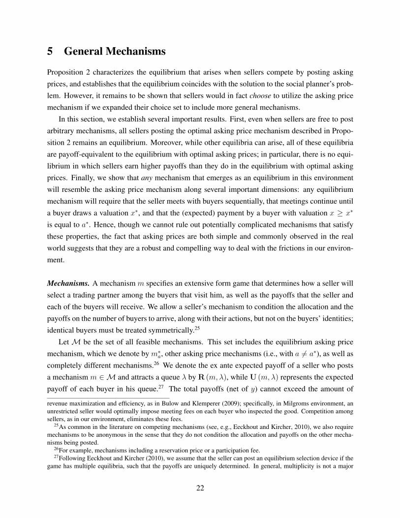
Mechanisms. A mechanism m specifies an extensive form game that determines how a seller willselect a trading partner among the buyers that visit him, as well as the payoffs that the seller andeach of the buyers will receive. We allow a seller’s mechanism to condition the allocation and thepayoffs on the number of buyers to arrive, along with their actions, but not on the buyers’ identities;identical buyers must be treated symmetrically.25

Let M be the set of all feasible mechanisms. This set includes the equilibrium asking pricemechanism, which we denote by m∗a, other asking price mechanisms (i.e., with a 6= a∗), as well ascompletely different mechanisms.26 We denote the ex ante expected payoff of a seller who postsa mechanism m ∈ M and attracts a queue λ by R (m,λ), while U (m,λ) represents the expectedpayoff of each buyer in his queue.27 The total payoffs (net of y) cannot exceed the amount of

revenue maximization and efficiency, as in Bulow and Klemperer (2009); specifically, in Milgroms environment, anunrestricted seller would optimally impose meeting fees on each buyer who inspected the good. Competition amongsellers, as in our environment, eliminates these fees.

25As common in the literature on competing mechanisms (see, e.g., Eeckhout and Kircher, 2010), we also requiremechanisms to be anonymous in the sense that they do not condition the allocation and payoffs on the other mecha-nisms being posted.

26For example, mechanisms including a reservation price or a participation fee.27Following Eeckhout and Kircher (2010), we assume that the seller can post an equilibrium selection device if the

game has multiple equilibria, such that the payoffs are uniquely determined. In general, multiplicity is not a major

22

surplus S (m,λ) generated by the allocation implemented by the mechanism, which in turn cannotexceed the surplus created by the planner’s solution, S∗(λ) ≡ S(x∗, λ). That is,

R (m,λ) + λU (m,λ)− y ≤ S (m,λ) ≤ S∗(λ) (21)

for all m and λ.Clearly, Pareto optimality requires that the entire surplus be divided between the seller and the

buyers, so we restrict attention to mechanisms that satisfy the first condition in (21) with equal-ity. If the second condition in (21) also holds with equality, i.e., the mechanism creates the sameamount of surplus as the planner’s solution, we will call the mechanism surplus-maximizing.

Equilibrium. An equilibrium in this more general environment is a distribution of mechanismsm ∈ M and queue lengths λ ∈ R+ across sellers, along with a market utility U , such that (i)given U , each pair (m,λ) maximizes profits R (m,λ) subject to the constraint U (m,λ) = U ; and(ii) aggregating queue lengths across all sellers yields the total measure of buyers, θb. Given thisdefinition, we now establish that a mechanism m ∈ M is an equilibrium strategy if, and only if,it creates the same surplus and the same expected payoffs as the optimal asking price mechanismm∗a.

Proposition 3. A mechanism m ∈ M is an equilibrium strategy if, and only if, it is payoff-

equivalent to the optimal asking price mechanism, i.e., R (m,λ) = R (m∗a, λ) and U (m,λ) =

U (m∗a, λ).

Since the optimal asking price mechanism is surplus-maximizing, the following result is im-mediate.

Corollary 1. Any equilibrium mechanism m ∈M is surplus-maximizing.

The intuition behind Proposition 3 and Corollary 1 is illustrated in Figure 2. Consider a can-didate equilibrium with market utility U in which a seller posts a mechanism m1 and receives aqueue λ1 satisfying U = U(m1, λ1), yielding expected profits R(m1, λ1)−y = S(m1, λ1)−λ1U1.

INSERT FIGURE 2 HERE

The first result is that m1 must be surplus-maximizing. To see why, suppose it is not; that is,suppose S(m1, λ1) < S∗(λ1), corresponding to point 1 in Figure 2. This seller’s expected profitscorrespond to the intersection of the vertical axis with the line through point 1 that has slope U .One can see immediately that this cannot be consistent with equilibrium behavior. For example,

concern, since there always exist other mechanisms that implement the desired payoffs uniquely.

23

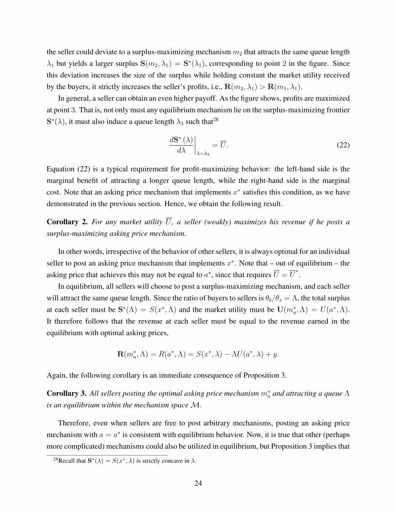
the seller could deviate to a surplus-maximizing mechanismm2 that attracts the same queue lengthλ1 but yields a larger surplus S(m2, λ1) = S∗(λ1), corresponding to point 2 in the figure. Sincethis deviation increases the size of the surplus while holding constant the market utility receivedby the buyers, it strictly increases the seller’s profits, i.e., R(m2, λ1) > R(m1, λ1).

In general, a seller can obtain an even higher payoff. As the figure shows, profits are maximizedat point 3. That is, not only must any equilibrium mechanism lie on the surplus-maximizing frontierS∗(λ), it must also induce a queue length λ3 such that28

dS∗ (λ)

dλ

∣∣∣∣λ=λ3

= U. (22)

Equation (22) is a typical requirement for profit-maximizing behavior: the left-hand side is themarginal benefit of attracting a longer queue length, while the right-hand side is the marginalcost. Note that an asking price mechanism that implements x∗ satisfies this condition, as we havedemonstrated in the previous section. Hence, we obtain the following result.

Corollary 2. For any market utility U , a seller (weakly) maximizes his revenue if he posts a

surplus-maximizing asking price mechanism.

In other words, irrespective of the behavior of other sellers, it is always optimal for an individualseller to post an asking price mechanism that implements x∗. Note that – out of equilibrium – theasking price that achieves this may not be equal to a∗, since that requires U = U

∗.

In equilibrium, all sellers will choose to post a surplus-maximizing mechanism, and each sellerwill attract the same queue length. Since the ratio of buyers to sellers is θb/θs = Λ, the total surplusat each seller must be S∗(Λ) = S(x∗,Λ) and the market utility must be U(m∗a,Λ) = U(a∗,Λ).It therefore follows that the revenue at each seller must be equal to the revenue earned in theequilibrium with optimal asking prices,

R(m∗a,Λ) = R(a∗,Λ) = S(x∗, λ)− ΛU(a∗, λ) + y.

Again, the following corollary is an immediate consequence of Proposition 3.

Corollary 3. All sellers posting the optimal asking price mechanism m∗a and attracting a queue Λ

is an equilibrium within the mechanism spaceM.

Therefore, even when sellers are free to post arbitrary mechanisms, posting an asking pricemechanism with a = a∗ is consistent with equilibrium behavior. Now, it is true that other (perhapsmore complicated) mechanisms could also be utilized in equilibrium, but Proposition 3 implies that

28Recall that S∗(λ) = S(x∗, λ) is strictly concave in λ.

24

any such mechanism will be similar to the asking price mechanism along several important dimen-sions. To start, since any equilibrium mechanism must be surplus-maximizing, and thus implementan allocation that coincides with the unique solution to the planner’s problem, the mechanism mustfeature sequential meetings between the seller and the buyers, with a stopping rule x∗ that dependsexplicitly on the realization of buyers’ valuations. Moreover, the mechanism must also allocate thegood to the agent with the highest valuation in the event that no agent draws a valuation x ≥ x∗.

Taken together, we see that any mechanism must have sequential meetings (ruling out anyform of static auction with simultaneous bidding) with some sort of device to elicit buyers’ privatevaluations, but this device must be flexible enough to allow the seller to return to each buyershould no other buyer reveal a valuation greater than x∗ (ruling out any form of take-it-or-leave-itoffers). These requirements place a fairly heavy burden on the mechanism’s design; the fact thatthis allocation can be achieved in a way that is both simple and familiar – with each seller postinga one-dimensional object a – suggests that asking prices are a natural way for sellers to deal withthe frictions in this environment.

Finally, since the ex ante probability that each buyer gets to meet with the seller must be equalin any equilibrium, and any mechanism that arises in equilibrium must also be payoff-equivalentto the equilibrium with optimal asking prices, it follows that the expected payment by buyerswith valuation x ∈ [x∗, x] must equal the optimal asking price. Therefore, even when sellersutilize an alternative mechanism in equilibrium, the expected transfer from a buyer who “stops”the sequential inspection process will, indeed, equal a∗. The following corollary summarizes.

Corollary 4. Any equilibrium strategy m ∈ M must specify that the seller meet with buyers

sequentially; that these meetings stop if, and only if, either the buyer draws a valuation x ≥ x∗ or

the end of the queue is reached; and that the expected payment for a buyer who draws valuation

x ≥ x∗ is equal to a∗.

6 Positive Implications

The theory developed above provides a compelling framework for studying markets in which ask-ing prices are prevalent. For one, the role of asking prices has explicit micro-foundations: byconsidering an environment in which buyers strategically choose which seller to visit, our frame-work produces an endogenous relationship between the asking prices set by sellers, the numberof buyers who arrive at each seller, their subsequent bidding behavior, and ultimately equilibriumprices and allocations. Moreover, as we showed in the previous section, this type of pricing schemeis not imposed exogenously, but rather it emerges as the optimal mechanism; that is, sellers choose

to use asking prices as an optimal response to the frictions in the market. Finally, despite the

25

relatively complex relationship between sellers’ asking prices, buyers’ search and bidding behav-ior, and the corresponding expected payoffs, the equilibrium is surprisingly simple and tractable.This tractability suggests that our framework could easily be incorporated into larger models (e.g.,macroeconomic models that include a housing sector) or extended to allow for various types ofheterogeneity (e.g., differentiated goods or preferences). Hence, we believe this model could be auseful benchmark for both theoretical and empirical work that focuses on markets in which askingprices are commonly used.

In this section, we flesh out some of the model’s implications for a variety of observable out-comes, including the level of asking prices set by the sellers, the number of buyers who inspect thegood at each seller, and the transaction price that is ultimately paid by the buyer who acquires thegood. We study how these variables change with features of the economic environment, such asthe ratio of buyers to sellers, the degree of ex ante uncertainty in buyers’ valuations, and the costsof inspecting the good.

Prices and Allocations. Figure 3 below plots a typical CDF of transaction prices, where we setb = 0 to represent sellers that do not trade.29 Notice that a fraction q0(y) = e−Λ[1−F (y)] of sellers donot trade, either because no buyers arrive, which occurs with probability q0(x) = e−Λ, or becausen ≥ 1 buyers arrive but their valuations do not exceed the seller’s valuation y, which occurs withprobability q0(y)−q0(x). A fraction q0(x∗)−q0(y) of sellers ultimately accept a bid b that is strictlyless than the asking price. Letting x(b) = b−1(x), where b(x) is defined in (11), the (cumulative)distribution of winning bids b ∈

[y, b(x∗)

)is simply q0 (x(b)) . Finally, a fraction 1 − q0(x∗) of

sellers trade at the asking price.

INSERT FIGURE 3 HERE

As we discussed above, notice that there is a mass point of transactions that occur at a∗ and a gapin the distribution between b(x∗) and a∗. Intuitively, it cannot be optimal for a buyer to offer aprice arbitrarily close to the asking price; such a strategy would be dominated by offering b = a∗,which would provide a discrete increase in the probability of trade, at the cost of an arbitrarilysmall increase in the terms of trade.

Comparative Statics. Figures 4 and 5 below illustrate how equilibrium prices are affected bychanges in the ratio of buyers to sellers (Λ) and changes in the inspection cost (k). An increase inΛ causes a decrease in the fraction of sellers who do not trade and an increase in the fraction ofsellers who trade at the asking price. Though x∗ is independent of Λ, notice that a∗ is not; it is easy

29For the sake of illustration, all numerical examples below have been generated with the assumption that x isuniformly distributed, though all of the results are true for arbitrary distributions.

26

to verify that a∗ is an increasing function of Λ. More generally, the distribution of prices under alarger Λ first-order stochastically dominates the distribution of prices under a smaller Λ. Hence, asin standard models of competitive search, an increase in the buyer-seller ratio leads to higher pricesin equilibrium. Notice, however, that the degree of dispersion in prices will be non-monotonic inΛ: though price dispersion exists for intermediate values of Λ, the equilibrium price distributionbecomes degenerate at b = y (b = x∗) as Λ converges to zero (infinity).

Alternatively, as the inspection cost k decreases, both the asking price a∗ and the cut-off x∗

increase. However, the buyers’ bidding function b(x) is unaffected, and hence the lower tail of theequilibrium price distribution is unaffected. As a result, a decrease in k leads to fewer transactionsat the asking price. Finally, as k converges to zero, the optimal x∗ converges to x and the pricingmechanism converges to a standard first-price auction.

INSERT FIGURES 4 and 5 HERE.

Information and Uncertainty. One might also be interested in the relationship between the ex antedispersion in buyers’ valuations, asking prices, and the ultimate transaction prices. For example,suppose a new technology (e.g., the Internet) replaces an old technology (e.g., the newspaper),allowing buyers to learn more information about each seller’s good before choosing a seller tovisit. Given this information, suppose now that a buyer can identify a fraction η of goods that hewould prefer, and a fraction 1−η of goods that he would not. Formally, a good that is preferred willyield a valuation x ∈ [x′, x], while a good that is not will yield the buyer a valuation x ∈ [x, x′],where x < x′ ≤ y < x. Whether or not a good is preferred is again i.i.d. across goods for eachbuyer.

One can easily show that buyers only visit preferred sellers and that the resulting equilibriumis very similar to what we characterize in Proposition 2, with the exception that the distribution Fwith support [x, x] is replaced by the truncated distribution F ′ with support [x′, x]. Figure 6 belowillustrates the main effects of this technological improvement.

INSERT FIGURE 6 HERE

First, notice that fewer sellers don’t trade, even though equilibrium queue lengths remain λ = Λ

at each seller. Intuitively, though the fraction of sellers who are visited by zero buyers remains con-stant, the truncated distribution implies that it is less likely for a seller to be visited by n ≥ 1 buyerswho all have a valuation strictly less than y. Second, notice that prices increase. This occurs forseveral reasons. For one, sellers set higher asking prices; on the margin, the expected gain frommeeting with an additional buyer is larger since the truncated distribution F ′ first-order stochasti-cally dominates the original distribution F . Moreover, since other buyers are more likely to drawa high valuation, there is more competition amongst buyers. This puts upward pressure on the

27

bidding function, causing further increases in transaction prices. Given these two facts, clearlysellers’ profits increase.

Prices and the Number of Inspections. In markets where asking prices are prevalent, the relation-ship between the sales price and the amount of time a good has been on the market has garneredsubstantial attention. Frequently, time itself is not really the object of interest, but rather it servesas a proxy for the number of meetings that occurred between a seller and potential buyers. Ourmodel has direct, testable implications for this relationship between the sales price and the numberof buyers who have inspected the good. Moreover, to the extent that each inspection might take acertain amount of time, our results could also be informative about the more indirect relationshipbetween sales price and time-on-the-market, which could be helpful when the number of buyerswho inspect the good is not directly observable.

Let p(i) denote the expected price of a good that was sold after i meetings. There are twopossible scenarios under which this event could occur. First, it could be the case that n ≥ i buyersarrived at this seller, the first i − 1 buyers had a valuation strictly less than x∗, and the ith buyerhad valuation x ≥ x∗. This occurs with probability

[1−

i−1∑

j=0

e−λλj

j!

]F (x∗)i−1 [1− F (x∗)] . (23)

Alternatively, it could be the case that exactly n = i buyers arrive, all of whom had valuationstrictly less than x∗, but at least one of whom had valuation x > y. This occurs with probability

e−λλi

i!

[F (x∗)i − F (y)i

]. (24)

In this case, the winning bid is given by b(x), where x is drawn from the conditional distribution

iF (x)i−1f(x)

F (x∗)i − F (y)i.

Therefore, the expected price of a good sold after i meetings is

p(i) =

[1−

∑i−1j=0

e−λλj

j!

]F (x∗)i−1 [1− F (x∗)] a∗ + e−λλi

i!

∫ x∗yiF (x)i−1f(x)b(x)dx

[1−

∑i−1j=0

e−λλj

j!

]F (x∗)i−1 [1− F (x∗)] + e−λλi

i![F (x∗)i − F (y)i]

. (25)

The relationship between the sales price and the number of meetings depends on the strength oftwo opposing forces. On the one hand, conditional on a seller not trading at the asking price,the maximum expected offer is increasing in i. This is a fairly obvious result: conditional on

28

all buyers’ valuations being strictly less than x∗, the distribution of the maximum offer amongst ibuyers first order stochastically dominates the distribution of the maximum offer amongst i′ buyersfor any i′ < i. This effect implies that p should be increasing in i. However, on the other hand,the probability that a seller does trade at the asking price, conditional on trading after i meetings,is decreasing in i.30 In words, as i gets larger, a trade that occurs after i meetings is more likelyto be the result of the seller exhausting the queue of buyers (and trading at a price less than a), asopposed to a trade that occurred because the ith buyer paid the asking price. This second effectimplies that p should be decreasing in i.

The strength of each of these effects varies across different values of i, which implies an in-teresting shape for p(i); figure 7 below provides a typical example. For small values of i, thelatter effect discussed above dominates; the conditional probability of trading at price a drops offrelatively quickly in the first few meetings. However, as i increases, this probability decreases ata much slower rate, and the positive effect of receiving more bids comes to dominate, causing theexpected transaction price to ultimately rise in i.

INSERT FIGURE 7 HERE

7 Assumptions and Extensions

In this section, we discuss several of our key assumptions, along with a few potentially interestingextensions of our basic framework.

Transactions Above the Asking Price. In the equilibrium characterized in section 4, no transactiontakes place at a price that exceeds the asking price. While we believe this prediction to be adequatefor certain markets, it is perhaps less desirable for the analysis of other markets.31 It is thereforeimportant to emphasize that our model can easily explain such transaction prices.32 To see this,note that one can interpret our asking price mechanism as a two-stage process in which the sellerfirst sequentially offers the good to each buyer at a price a∗ and then organizes a first-price auctionif no buyer accepts this offer. Given proposition 3 and standard revenue-equivalence results, analternative, optimal mechanism would be to replace the first-price auction with a second-priceauction in the second stage of the game.

Note that such a mechanism has a natural interpretation in the context of a housing market. Itcorresponds to a scenario in which a seller, after getting a number of offers which are all below

30Note that this probability is easy to calculate, given the expressions in (23) and (24).31For example, Case and Shiller (2003) and Han and Strange (2013) provide evidence for a variety of cities in which

houses occasionally sell above the asking price.32We would like to thank Rob Shimer for pointing out this feature of our model.

29

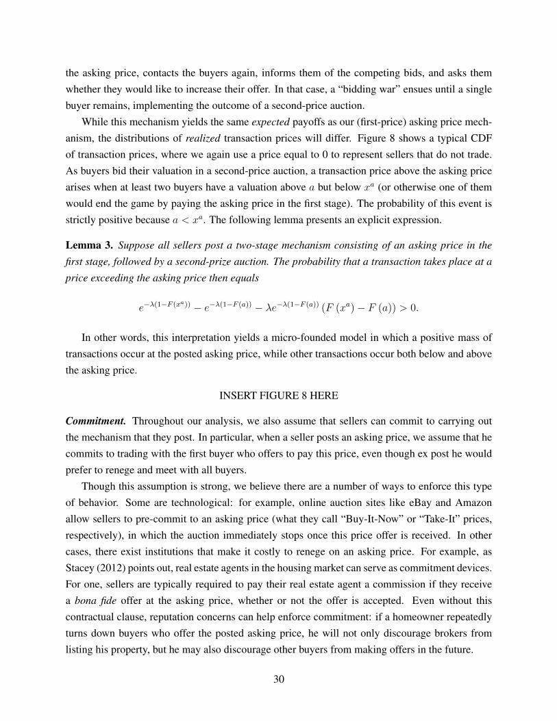
the asking price, contacts the buyers again, informs them of the competing bids, and asks themwhether they would like to increase their offer. In that case, a “bidding war” ensues until a singlebuyer remains, implementing the outcome of a second-price auction.

While this mechanism yields the same expected payoffs as our (first-price) asking price mech-anism, the distributions of realized transaction prices will differ. Figure 8 shows a typical CDFof transaction prices, where we again use a price equal to 0 to represent sellers that do not trade.As buyers bid their valuation in a second-price auction, a transaction price above the asking pricearises when at least two buyers have a valuation above a but below xa (or otherwise one of themwould end the game by paying the asking price in the first stage). The probability of this event isstrictly positive because a < xa. The following lemma presents an explicit expression.

Lemma 3. Suppose all sellers post a two-stage mechanism consisting of an asking price in the

first stage, followed by a second-prize auction. The probability that a transaction takes place at a

price exceeding the asking price then equals

e−λ(1−F (xa)) − e−λ(1−F (a)) − λe−λ(1−F (a)) (F (xa)− F (a)) > 0.

In other words, this interpretation yields a micro-founded model in which a positive mass oftransactions occur at the posted asking price, while other transactions occur both below and abovethe asking price.

INSERT FIGURE 8 HERE

Commitment. Throughout our analysis, we also assume that sellers can commit to carrying outthe mechanism that they post. In particular, when a seller posts an asking price, we assume that hecommits to trading with the first buyer who offers to pay this price, even though ex post he wouldprefer to renege and meet with all buyers.

Though this assumption is strong, we believe there are a number of ways to enforce this typeof behavior. Some are technological: for example, online auction sites like eBay and Amazonallow sellers to pre-commit to an asking price (what they call “Buy-It-Now” or “Take-It” prices,respectively), in which the auction immediately stops once this price offer is received. In othercases, there exist institutions that make it costly to renege on an asking price. For example, asStacey (2012) points out, real estate agents in the housing market can serve as commitment devices.For one, sellers are typically required to pay their real estate agent a commission if they receivea bona fide offer at the asking price, whether or not the offer is accepted. Even without thiscontractual clause, reputation concerns can help enforce commitment: if a homeowner repeatedlyturns down buyers who offer the posted asking price, he will not only discourage brokers fromlisting his property, but he may also discourage other buyers from making offers in the future.

30

For all of these reasons, we think that the assumption of full commitment is a reasonable ap-proximation of the way goods are sold in certain markets. Of course, there are other markets inwhich sellers may not be able to commit to such a device; extending our framework to allow forlimited commitment, or even no commitment (as in Kim and Kircher, 2012), could potentiallyallow our model to capture these features as well. This extension is left for future work.33

Endogenous Inspection. Throughout the text we assumed that buyers inspect the good and learntheir valuation before submitting a bid. One interpretation of this assumption is that it is a techno-logical constraint: a buyer simply must go and meet with the seller in order to make an offer (say,he needs to sign certain documents), and this process is costly.

However, for many applications it may be more appropriate to treat the decision to inspect thegood as endogenous. In such an environment, if the inspection cost k becomes too large, there mayexist states of the world in which the buyer (or the planner) prefers to forgo inspection and placea bid (or trade) without knowing the valuation. The following lemma derives a condition on k toensure that this is never the case. That is, under the condition below, inspection before submittinga bid or trading is optimal both for the planner and for the buyers in the decentralized market.

Lemma 4. The planner always instructs buyers to inspect the good upon meeting a seller and, in

the decentralized equilibrium, buyers always choose to inspect the good before submitting a bid if

and only if

k <

∫ y

x

(y − x) f (x) dx. (26)

Hence, the analysis in Sections 3 and 4 is consistent with an environment in which the decisionto inspect the good is endogenous, but k is sufficiently small to satisfy (26). In words, this inequal-ity implies that inspection is always optimal as long as the cost of inspecting is smaller than thecosts associated with inefficient trade, which occurs when the seller values the good more than thebuyer who receives it. Before proceeding, we highlight two important points regarding (26). First,inspection will, in general, almost always remain an optimal strategy for buyers in large regionsof the parameter space that do not satisfy this condition. Second, for most of the goods we havein mind (e.g., a house or a car), the assumption that the inspection cost k is small relative to thepotential gains (or losses) from trade seems to be appropriate.

Free Entry. A third assumption that we discuss is our restriction to a fixed ratio of buyers to sellers.Though Proposition 2 establishes that the equilibrium cutoff xa is efficient in our environment, a

33A stylized but particularly tractable approach would be to assume that, after the arrival of the buyers, the sellercan renege on the asking price at a certain cost or in certain states of the world. This would not only allow our modelto accommodate transaction prices above the asking price, but it would also create a natural intermediate case betweenour framework and the model by Albrecht et al. (2012a).

31

traditional concern in much of the search literature is whether efficiency is also achieved when theratio of buyers to sellers is determined endogenously.

To address this issue, suppose that sellers can freely enter the market by paying a cost c, as instandard search models (see, e.g., Pissarides, 1985). The planner will then choose Λ to maximizenet social surplus, maxΛ∈(0,∞)

θbΛ

[S (x∗,Λ)− c], while the equilibrium buyer/seller ratio followsfrom the indifference condition R (a∗,Λ) − c = y. In the appendix, we show that the markettightness achieved in equilibrium indeed coincides with the solution to the planner’s problem.

Lemma 5. The market equilibrium with free entry is constrained efficient.

Heterogeneous Inspection Costs. We chose to endogenize the number of buyers at each sellerby studying a model of directed search, where a large number of sellers compete for buyers, andbuyers choose strategically among these sellers. In this setting, a buyer ultimately pays two costsbefore acquiring a good: the inspection cost, which we discussed at length above, as well asan opportunity cost of visiting the seller (instead of a different seller), which is the equilibriummarket utility U . An alternative approach would have been to consider a single seller and replacethe endogenous opportunity cost with an exogenous entry cost. Within our benchmark model,this alternative would have yielded essentially the same results: a simple asking price would haveensured that the socially optimal number of buyers would have visited the monopolistic seller, andthat the socially optimal number of buyers would have inspected the good.

However, if we relax the assumption that buyers are homogeneous, then casting our environ-ment within a model of directed search provides a distinct advantage, as the possibility of endoge-nous market segmentation emerges. This could help to explain why identical sellers would postdifferent asking prices, or even use different mechanisms altogether. As a result, some goods wouldsell “quickly” (i.e., with high probability) at lower prices, while other goods would sell slowly athigher prices.

For example, suppose buyers are heterogeneous with respect to their inspection costs: a fractionφ ∈ (0, 1) of buyers have inspection cost k1 while the remaining buyers have inspection cost k2,with k2 > k1 > 0. Then, as the following lemma reports, a separating equilibrium arises in whichbuyers sort themselves into different submarkets on the basis of their cost. In one submarket,sellers post low asking prices, which attract the buyers with high inspection costs, since they placea premium on reducing the risk of a fruitless inspection. In the other submarket, sellers post higherasking prices and serve the buyers with low inspection costs; in the limit, as these inspection costsconverge to zero, the mechanism at these sellers converges to a standard auction.34 In order to

34In this sense, our work is related to Eeckhout and Kircher (2010). By studying various exogenous meetingtechnologies, they analyze how the degree of crowding out (‘rivalry’) in meetings between buyers and sellers affects

32

ensure that sellers are indifferent between these two mechanisms, the queue length adjusts: thesellers posting low asking prices attract relatively longer queue lengths and sell quickly.

Lemma 6. In a market with two types of buyers, with 0 < k1 < k2, there exists an asking price

equilibrium with two submarkets. In each submarket i ∈ {1, 2}, sellers post asking price ai and

attract a queue length λi that consists of only buyers with inspection cost ki, which implements a

stopping rule xai . This equilibrium is efficient and has the following properties: a1 > a2, xa1 > xa2,

and λ1 < λ2.

This simple example highlights one dimension along which the model could be easily extendedto confront empirical regularities in the data, such as heterogeneous asking prices or time-on-the-market, along with the coexistence of identical goods being sold with different pricing mecha-nisms.35

8 Conclusion

In the majority of existing economic models, it is assumed that either (i) non-negotiable prices areset by sellers; (ii) prices are the outcome of a bargaining game between a single buyer and seller;or (iii) prices are determined through an auction. However, many goods (and services) are soldin a manner that is not consistent with any of these three pricing mechanisms, but rather seemsto combine elements of each. First, sellers announce a price, as in models with price-posting, atwhich they’re willing to sell their good or service immediately. However, as in bargaining theory,buyers can submit a counteroffer that will also be considered by the seller. Finally, in the eventthat no buyer offers the asking price within a certain period of time, the set of counteroffers thatthe seller has received are aggregated, as in an auction, and the object is awarded to the buyer withthe best counteroffer.

Despite the prevalence of this pricing scheme in many markets, it has received little attentionin the academic literature. Without a coherent theory, it’s hard for economists to identify theunderlying cause for observed changes in prices and allocations in these markets, or to forecast theeffects of future shocks. For example, in real estate markets, the ratio of sales prices to list pricesvaries widely across locations and can often change significantly over time; the three standardpricing mechanisms described above simply offer no way to interpret data of this sort.

the optimal sales mechanism. While crowding out always reduces welfare in their environment, we show that it mayarise endogenously as the optimal response to the existence of inspection costs. Although our environment is quitedifferent from theirs, we also find that the optimal sales mechanism is sometimes an auction and sometimes a postedprice. In addition, we show that the asking price mechanism convexifies the range between these two extremes.

35Other forms of heterogeneity, e.g. observable differences in sellers’ own valuations, will often also lead to aseparating equilibrium in which each submarket looks exactly as derived in section 4.

33

In this paper, our objective was to construct a sensible economic model to help us understandhow and why this type of pricing mechanism can be an efficient way of selling goods and services.Combining two simple, realistic ingredients — namely, competition and costly inspection — weshowed that asking prices emerge as the mechanism that is both revenue-maximizing and efficient.As a result, the framework developed here provides a theory of asking prices that is both micro-founded and tractable, offers a variety of testable predictions, and lends itself easily to variousextensions. Given these features, we believe that our model could be useful for both theoreticaland empirical work that focuses on markets in which asking prices are commonly used.

34

Appendix

Proof of Lemma 1. In general, if n buyers arrive at a seller, the planner might want to first learnthe valuations of i1 ≤ n buyers simultaneously at cost i1k. Then, depending on the realization(x1, ..., xi1), the planner could choose to either allocate the good to one of these i1 buyers (or theseller), or alternatively the planner could choose to continue and sample i2 ≤ n − i1 buyers, inwhich case this iterative process would continue. This is precisely a special case of the problemthat Morgan and Manning (1985) study, so we sketch the intuition for our result below and referthe reader to their paper for a more rigorous treatment.

To see that it can never be optimal to learn the valuation of more than one buyer at a time,suppose n buyers arrive at a seller, and consider the planner’s decision of whether to learn thevaluations of the first two buyers sequentially or simultaneously. Let Zi(xi) − y denote the netexpected surplus from continuing to learn buyers’ valuations (under the optimal policy) given thatthe maximum valuation of the seller and the i buyers sampled so far is xi ≡ max {y, x1, . . . , xi}.

We will show that, for any realizations of the first two buyers’ valuations (x1, x2), the net socialsurplus is weakly larger from learning these two valuations sequentially than it is from learningthem simultaneously. To see this, realize that the net social surplus from learning these valuationssimultaneously is

−2k − y + max {x2, Z2 (x2)} , (27)

whereas the surplus from learning these valuations sequentially is

−k − y + max {x1,−k + max {x2, Z2 (x2)}}

= −2k − y + max {x1 + k, x2, Z2 (x2)} (28)

Clearly, the expression in (28) is weakly larger than (27) for any x1 and x2, and strictly larger forsome x1 and x2. Taking the expectation over all possible realizations therefore implies that a plan-ner would want to learn these valuations sequentially ex ante. It is straightforward to extend thisargument to learning the valuations of m > 2 buyers simultaneously after any number i ≤ n−mbuyers have already inspected the good. �

Proof of Lemma 2. The proof of Lemma 2 utilizes an induction argument. We begin with thefirst step. If the seller has met with all n buyers, the decision is trivial: the good is allocatedto the agent (either one of the buyers or the seller) with valuation xn. The expected surplus isVn,n(xn) = xn− y. As in the text, to economize on notation we will drop the second subscript “n”below, so that Vi,n(xi) ≡ Vi(xi), xpi,n ≡ xpi , and so on.

Working backward, consider the planner’s problem when the seller has met with only n − 1

35

of the n buyers. If the planner instructs the seller to stop meeting with buyers, again the good isallocated to the agent with valuation xn−1, yielding surplus xn−1 − y. Alternatively, if the sellermeets with the next buyer, the expected surplus is Zn−1(xn−1)− y, where

Zn−1(x)− y = −k +

∫ x

x

max {Vn (x) , Vn (x)} f (x) dx,

so that

Zn−1(x) = −k + xF (x) +

∫ x

x

xf (x) dx. (29)

Notice immediately that Zn−1(x∗) = x∗ and dZn−1(x)x

= F (x) ∈ (0, 1), so that clearly xpn−1 =

x∗ is the optimal cutoff after meeting with n− 1 buyers, and

Vn−1 (x) =

x− y for x ≥ x∗

Zn−1 (x)− y for x < x∗.

Now consider the planner’s problem after the seller has met with n − 2 buyers. We establishthree important properties of Zn−2(x): (1) Zn−2(x) = Zn−1(x) for all x ≥ x∗; (2) Zn−2(x) > x

for all x < x∗; and (3) limx→x∗ Zn−2(x) = Zn−1(x∗) = x∗. Given these three properties, alongwith the fact that dZn−2(x)

x= dZn−1(x)

x= F (x) ∈ (0, 1) for x ≥ x∗, it follows immediately that

x ≥ Zn−2(x) if, an only if, x ≥ x∗, and hence xpn−2 = x∗ is optimal.After meeting with n− 2 buyers, the expected surplus from another meeting when xn−2 = x is

Zn−2 (x)− y = −k + Vn−1 (x)F (x) +

∫ x

x

Vn−1 (x) f (x) dx. (30)

If x ≥ x∗, then Vn−1 (x) = x − y and thus Zn−2 (x) = Zn−1 (x). Alternatively, if x < x∗, thenVn−1 (x) = Zn−1 (x)− y > x− y and

Zn−2 (x) = −k + Zn−1 (x)F (x) +

∫ x∗

x

Zn−1 (x) f (x) dx+

∫ x

x∗xf (x) dx

> −k + xF (x) +

∫ x∗

x

xf (x) dx+

∫ x

x∗xf (x) dx

= Zn−1 (x) > x.

36

Finally, note that

limx→x∗

Zn−2 (x) = −k + Zn−1 (x∗)F (x∗) +

∫ x

x∗xf (x) dx

= −k + x∗F (x∗) +

∫ x

x∗xf (x) dx

= Zn−1(x∗) = x∗.

Therefore, the optimal cutoff after meeting with n− 2 buyers is x∗n−2 = x∗.We have established that the following is true for j′ = 2:

1. Zn−j′(x) = Zn−j′+1(x) for all x ≥ x∗.

2. Zn−j′(x) > x for all x < x∗.

3. limx→x∗ Zn−j′(x) = Zn−j′+1(x∗) = x∗,

so that

Vn−j′ (x) =

x− y for x ≥ x∗

Zn−j′ (x)− y for x < x∗.

Now, suppose this is true for all j′ ∈ {2, 3, ..., j}. We will establish that it is also true for j + 1.After meeting with n− j− 1 buyers, the expected surplus from another meeting when xn−j−1 = x

is

Zn−j−1 (x)− y = −k + Vn−j (x)F (x) +

∫ x

x

Vn−j (x) f (x) dx. (31)

If x ≥ x∗, then Vn−j (x) = x − y and thus Zn−j−1 (x) = Zn−1 (x). Moreover, given the firstassumption in the induction step, Zn−j (x) = Zn−1 (x), so that Zn−j−1 (x) = Zn−j (x).

Alternatively, if x < x∗, then

Zn−j−1 (x) = −k + Zn−j (x)F (x) +

∫ x∗

x

Zn−j (x) f (x) dx+

∫ x

x∗xf (x) dx

> −k + xF (x) +

∫ x

x

xf (x) dx = Zn−1 (x) > x

Finally, note that

limx→x∗

Zn−j−1 (x) = −k + Zn−j (x∗)F (x∗) +

∫ x

x∗xf (x) dx

= Zn−1(x∗) = x∗.

37

Therefore, we have that the optimal cutoff after meeting with n− j − 1 buyers is xpn−j−1 = x∗. �

Proof of Proposition 1. Given the results in Lemmas 1 and 2, all that remains to be shown is thatit is optimal to assign queue lengths λ = Λ at each seller. Substituting (2) into (6) and integratingby parts yields

S (x∗, λ) = x∗ − y −∫ x∗

y

q0 (x) dx.

Since x∗ is independent of λ, the second derivative of S (x∗, λ) with respect to λ then equals

d2S

dλ2= −

∫ x∗

y

(1− F (x))2 q0 (x) dx < 0.

Hence, the surplus generated by a seller is strictly concave in the queue length. Total surplus istherefore maximized by assigning the same queue length λ = Λ to all sellers. �

Proof of Proposition 2. Since the relation between a and xa is one-to-one, given λ, the seller’smaximization problem can be rewritten as a choice over xa and λ, which turns out to be moreconvenient analytically. Define R (xa, λ) as the revenue of a seller with asking price a, queue λand cutoff xa ≡ xa (a, λ). Substituting b (x) from (11) and a from (14) into R (a, λ), as given in(16), yields

R (xa, λ) = xa − (1 + λ)

∫ xa

y

q0 (x) dx+ λ

∫ xa

y

F (x) q0 (x) dx.

One can derive U (xa, λ), i.e., the expected payoff of a buyer visiting this seller, in a similar fashion:

U (xa, λ) =1

λ

(1− q0(xa)

(1− F (xa))

[∫ x

xa(x− xa) dF (x)− k

]+ λ

∫ xa

y

(1− F (x)) q0 (x) dx

).

(32)The partial derivatives of R (xa, λ) are equal to

∂R

∂xa= 1−Q1(xa) > 0

∂R

∂λ= λ

∫ xa

y

(1− F (x))2 q0 (x) dx > 0

38

while the partial derivatives of U (xa, λ) are

∂U

∂xa= −1−Q1(xa)

λ

(1− f (xa)

(1− F (xa))2

[∫ x

xa(x− xa) dF (x)− k

])< 0

∂U

∂λ= − 1−Q1(xa)

λ2 (1− F (xa))

[∫ x

xa(x− xa) dF (x)− k

]−∫ xa

y

q0 (x) (1− F (x))2 dx,

since Q1(xa) < 1. Therefore, the first-order conditions of the Lagrangian with respect to xa, λ,and µ, respectively, equal

0 = (1−Q1(xa))

(1− µ

λ

(1− f (xa)

(1− F (xa))2

[∫ x

xa(x− xa) dF (x)− k

]))(33)

0 = λ

∫ xa

y

q0 (x) (1− F (x))2 dx(

1− µ

λ

)

− µ

λ2

1−Q1(xa)

(1− F (xa))

[∫ x

xa(x− xa) dF (x)− k

](34)

0 =1− q0(xa)

λ (1− F (xa))

[∫ x

xa(x− xa) dF (x)− k

]+

∫ xa

y

(1− F (x)) q0 (x) dx− U.

Solving (33) implies

µ

λ=

(1− f (xa)

(1− F (xa))2

[∫ x

xa(x− xa) dF (x)− k

])−1

,

so that (34) can be written as

0 =

[∫ x

xa(x− xa) dF (x)− k

]×

µ

λ

{−λf (xa)

∫ xayq0 (x) (1− F (x))2 dx

(1− F (xa))2 − 1−Q1(xa)

λ (1− F (xa))

}.

Since the term in brackets on the second line of this equation is strictly negative, it must be thatthe unique solution for xa satisfies

∫ xxa

(x− xa) dF (x) = k. From this, it immediately follows thatxa = x∗ and µ = λ = Λ. Hence, the equilibrium is unique and it coincides with the solution to theplanner’s problem. Given xa = x∗ and λ = Λ, the optimal asking price follows from (14). �

Proof of Proposition 3. Consider a candidate equilibrium in which one or more sellers posta particular trading mechanism m1 and attract a queue λ1 > 0, which yields them a payoffR (m1, λ1), yields the buyers a market utility U ≡ U (m1, λ1), and creates a surplus S (m1, λ1) =

39

R (m1, λ1) + λ1U (m1, λ1) − y. Equilibrium requires that no profitable deviation exists. Hence,a deviant seller who posts a mechanism m3 and attracts a queue λ3, determined by market utility,must obtain a weakly lower payoff, i.e., R (m3, λ3) ≤ R (m1, λ1) for all m3 and λ3 such thatU (m3, λ3) = U .

Using the definition of S (m3, λ3), the deviant’s payoff equals

R (m3, λ3) = S (m3, λ3)− λ3U + y.

This payoff is maximized when the deviant chooses a surplus-maximizing mechanism which issuch that λ3 satisfies the first-order condition

d

dλS∗ (λ)

∣∣∣∣λ=λ3

= U. (35)

As follows from previous results, an asking price that implements the cutoff x∗ satisfies this con-dition and is therefore a solution to the deviant’s maximization problem.

Note that (m1, λ1) can be part of an equilibrium if, and only if, it is a solution to the deviant’smaximization problem, i.e., m1 is surplus-maximizing and λ1 solves (35). Since S∗ (λ) is strictlyconcave, a unique solution exists to (35) for each level of market utility. Hence, all sellers mustattract the same queue length and this queue length must equal λ = Λ, since any other value wouldbe inconsistent with the aggregate buyer-seller ratio. Since d

dλS∗ (λ)

∣∣λ=Λ

= U (m∗a,Λ), this im-plies that a mechanism m is an equilibrium strategy if and only if it creates the same surplus asthe optimal asking price mechanism as well as the same payoff for the buyers. Equivalence of theseller’s payoff then follows immediately. �

Proof of Lemma 3. Consider a seller with n buyers. The sale price will be above asking price ifi ∈ {2, . . . , n} buyers draw a valuation between a and xa while the remaining n− i buyers draw avaluation below a. The probability of this event equals

n∑

i=2

n!

i! (n− i)!(F (xa)− F (a))i F (a)n−i ,

which simplifies to

F (xa)n − n (F (xa)− F (a))F (a)n−1 − F (a)n .

Taking the expectation over n yields the desired expression. �

40

Proof of Lemma 4. For the planner’s problem, the proof proceeds by induction, much like theproof of lemma 2. Suppose that n buyers visit a seller, the first n− 1 buyers learn their valuation,and no trade has taken place because xn−1 ≡ max {y, x1, . . . , xn−1} < x∗. In this case, the plannerhas two options: either let buyer n incur the inspection cost k and base the ensuing trading decisionon xn, or avoid the inspection cost by instructing the seller to trade with buyer n without knowinghis valuation.36

In the former case, expected surplus generated by the match is Zn−1 (xn−1)− y, where

Zn−1(x) = −k + xF (x) +

∫ x

x

xf (x) dx,

while the latter case yields an expected surplus equal to∫ xxxf (x) dx − y. Clearly, inspection is

preferred if and only if Zn−1 (xn−1)− y >∫ xxxf (x) dx− y, or equivalently

k <

∫ xn−1

x

(xn−1 − x) f (x) dx.

This condition needs to hold for any feasible value of xn−1 in order to guarantee inspection by thelast buyer. Since the right-hand side is strictly increasing in xn−1, (26) is a necessary and sufficientcondition. The final step is then to show that this condition implies that inspection is also optimalafter meeting with n − j − 1 buyers for j ∈ {1, . . . , n− 1}. This follows immediately fromZn−j−1 (x) ≥ Zn−1 (x) for all x and j, as shown in the proof of lemma 2.

Next, we analyze the market equilibrium described in section 4. Consider a deviating buyerwho does not inspect the good and therefore does not know his valuation. This deviant has threeoptions: 1) submit a bid below y, which will be rejected; 2) submit a bid between y and a; or3) bid the asking price and trade immediately. The choice between these options is equivalent tochoosing a type of buyer x′ ∈ [x, x] to mimic.

We first establish that it is optimal for the deviant to behave like a buyer who has a valuation x′

equal to the unconditional expected value of x, which we denote by xe = EF [x] ≡∫ xxxf (x) dx.

To see this, consider the expected payoffs under each of the three options. First, a deviant who actslike a buyer with valuation x′ ∈ [x, y] receives a payoff of 0. Second, if the deviant instead imitatesa buyer of type x′ ∈ (y, xa) and bids b (x′), his payoff conditional on meeting with the seller is

u(x′|xe) =λ (1− F (xa)) q0(x′)

1− q0(xa)

[xe − b(x′)

].

36The planner can of course also instruct the seller to immediately trade with the agent with valuation xn−1, but, asshown in lemma 2, this is dominated by learning the valuation of the last buyer since xn−1 < x∗.

41

Since b (x′) is optimal in equilibrium, it follows that the deviant should choose x′ = xe and bidb (xe). Evaluating the expected payoff from this strategy yields

u (xe) =λ (1− F (x∗))

1− q0(x∗)

∫ xe

y

q0 (x) dx, (36)

where u (xe) is increasing and convex in its argument. Finally, if the deviant mimics a buyer oftype x′ ∈ [x∗, x] and bids the asking price, he obtains a payoff

xe − a∗ = xe − x∗ + u (x∗) . (37)

Comparing the three payoffs reveals that the deviant maximizes his payoff by behaving as abuyer with valuation xe. That is, he should submit a bid below y if xe < y and should bid b (xe) ifxe ∈ [y, x∗). Note that the remaining case, xe ∈ [x∗, x], cannot occur under (26), since it implies

xe = −∫ x∗

x

(x∗ − x) f (x) dx+ k + x∗

< −∫ y

x

(y − x) f (x) dx+ k + x∗ < x∗.

To see whether the deviant benefits from not inspecting the good, define an auxiliary distribu-tion F (x) that resembles F (x), except that the mass below y and above x∗ is concentrated as masspoints at y and x∗, respectively. That is,

F (x) =

0 if x < y

F (x) if y ≤ x ≤ x∗

1 if x∗ < x.

Let xe = EF [x] denote the expectation of x under this modified distribution. Under (26), it thenfollows that xe > xe, since

xe − xe =

∫ y

x

(y − x) dF (x)−∫ x

x∗(x− x∗) dF (x)

=

∫ y

x

(y − x) dF (x)− k > 0.

The fact that u (x) is an increasing function then implies that u (xe) < u (xe), while the convex-ity of u (x) implies that u (xe) < EF [u (x)] by Jensen’s inequality. Note, however, that EF [u (x)]

42

exactly equals the payoff from inspection, since

EF [u (x)] = u (y) F (y) +

∫ x∗

y

u (x) dF (x) +(

1− F (x∗))u (x∗)

=

∫ x∗

y

u (x) dF (x) + (1− F (x∗))u (x∗)

=λ (1− F (xa))

1− q0 (xa)

[∫ x∗

y

∫ x

y

q0 (x) dxdF (x) + (1− F (x∗))

∫ x∗

y

q0 (x) dx

]

Hence, the payoff from inspection is strictly higher than the payoff from not inspecting.To show that equation (26) is also necessary, consider the limit Λ → 0, such that a buyer who

meets with a seller knows that, with probability 1, he does not face competition from other buyers.The optimal bid in that case is y and it follows immediately that inspection is better only if equation(26) holds.

�

Proof of Lemma 5. The equilibrium buyer-seller ratio is determined by the free entry conditionR (x∗,Λ)− c = y. Since S (x∗, λ) = R (x∗, λ) + λU (x∗, λ)− y, this condition is equivalent to

S (x∗,Λ)− c = ΛU (x∗,Λ) . (38)

The efficient buyer-seller ratio follows from the first-order condition of net social surplusθbΛ

[S (x∗,Λ)− c] with respect to Λ. After simplification, this yields

− 1

Λ[S (x∗,Λ)− c] +

∂

∂λS (x∗,Λ) = 0. (39)

Since ∂∂λS (x∗,Λ) = U (x∗,Λ), it follows that the solution to (38) solves (39). �

Proof of Lemma 6. The first part of this proof closely resembles the proof of proposition 2,although we focus on the ‘dual’ problem, i.e., the buyers’ maximization problem. Let R (xa, λ)

denote a seller’s revenue given a cutoff xa and a queue λ. Similarly, let Ui (xa, λ) denote thecorresponding payoff of a buyer with inspection cost ki. The Lagrangian for a buyer of type i is

Li (xa, λ, ψ) = Ui (xa, λ) + ψ

(R (xa, λ)−R

),

where ψ is the multiplier on the constraint requiring that sellers only offer combinations of (xa, λ)

that provide them with their equilibrium payoff R. The FOCs of this Lagrangian with respect toxa and λ correspond to the ones in the proof of proposition 2 for ψ = 1

µ. They therefore imply

43

∫ xxa

(x− xa) dF (x) = ki. Let xai denote the cutoff that solves this equation. Then clearly xa1 > xa2.A pooling equilibrium in this environment would require that all sellers post the same asking

price a and attract the same queue length Λ, consisting of both types of buyers. However, thisasking price and queue length cannot simultaneously implement both xa1 and xa2. Hence, a poolingequilibrium does not exist. A similar argument rules out partial pooling.

Instead, a separating equilibrium with two submarkets must arise, in which a fraction of sellerspost an asking price ai that attracts only buyers with inspection cost ki, for i ∈ {1, 2}. Theequilibrium queue length at each type of seller, λi, will then imply the cutoff xai described above.Since a seller’s revenue is strictly increasing in both his cutoff and queue length (see again theproof of proposition 2), the seller’s indifference condition implies that the queue length must beshorter in the submarket with the higher cutoff, i.e., λ1 < λ2.

Having established that xa1 > xa2 and λ1 < λ2, in equilibrium, it remains to be shown thata1 > a2. Suppose, towards a contradiction, that a2 ≥ a1. The equilibrium revenue R2 for sellersin the submarket that implements xa2 then equals

R2 = yq0 (y;λ2) +

∫ xa2

y

b (x;λ2) dq0 (x;λ2) +

∫ xa1

xa2

a2dq0 (x;λ2) +

∫ x

xa1

a2dq0 (x;λ2) ,

where λ is (re-)introduced as an argument of the functions b(·) and q0(·) to avoid ambiguity.Note that given a particular cutoff, revenue is strictly increasing in the queue length and the

asking price. Note further that the asking price a1 must exceed b (xa1). Hence,

R2 > yq0 (y;λ1) +

∫ xa2

y

b (x;λ1) dq0 (x;λ1) +

∫ xa1

xa2

a1dq0 (x;λ1) +

∫ x

xa1

a1dq0 (x;λ1)

> yq0 (y;λ1) +

∫ xa2

y

b (x;λ1) dq0 (x;λ1) +

∫ xa1

xa2

b (x;λ1) dq0 (x;λ2) +

∫ x

xa1

a1dq0 (x;λ1)

= R1,

where R1 denotes the equilibrium revenue for sellers in the submarket that implements xa1. Thisyields the desired contradiction. Hence, a1 > a2.

Conditional on separation, the efficiency of xa1 and xa2 immediately follows earlier results.Hence, the only thing left to prove is that the planner indeed prefers separation over pooling.If the planner pools both types of buyers, then ex post the optimal cutoff xp is the solution to∫ xxp

(x− xp) dF (x) = φk1 + (1− φ)k2. Output in that case equals θsS (xp,Λ).When the planner separates the buyer types into submarkets with cutoffs x∗1 and x∗2 instead, he

needs to decide how many sellers to allocate to each submarket. Let η denote the fraction of sellers

44

assigned to the submarket with xa1. Optimal output then equals

maxηηθsS

(x∗1,

φ

ηΛ

)+ (1− η)θsS

(x∗2,

1− φ1− η

Λ

).

Separation creates more output than pooling, since

maxηηθsS

(x∗1,

φ

ηΛ

)+ (1− η)θsS

(x∗2,

1− φ1− η

Λ

)

> maxηηθsS

(xp,

φ

ηΛ

)+ (1− η)θsS

(xp,

1− φ1− η

Λ

)

> θsS (xp,Λ) .

�

45

ReferencesAcemoglu, D. and Shimer, R. (1999). Efficient unemployment insurance. Journal of Political

Economy, 107:893–928.

Albrecht, J. W., Gautier, P. A., and Vroman, S. B. (2012a). Directed search in the housing market.mimeo.

Albrecht, J. W., Gautier, P. A., and Vroman, S. B. (2012b). A note on Peters and Severinov,“Competition among sellers who offer auctions instead of prices”. Journal of Economic Theory,147:389–392.

Arnold, M. A. (1999). Search, bargaining and optimal asking prices. Real Estate Economics,27(3):453–481.

Bajari, P. and Hortacsu, A. (2003). The winner’s curse, reserve prices, and endogenous entry:Empirical insights from eBay auctions. RAND Journal of Economics, 34(2):329–55.

Budish, E. B. and Takeyama, L. N. (2001). Buy prices in online auctions: Irrationality on theinternet? Economics Letters, 72:325–333.

Bulow, J. and Klemperer, P. (2009). Why do sellers (usually) prefer auctions? American EconomicReview, 99(4):1544–1575.

Burdett, K., Shi, S., and Wright, R. (2001). Pricing and matching with frictions. Journal ofPolitical Economy, 109:1060–1085.

Burguet, R. (1996). Optimal repeated purchases when sellers are learning about costs. Journal ofEconomic Theory, 68(2):440–455.

Burguet, R. and Sakovics, J. (1999). Imperfect competition in auction designs. InternationalEconomic Review, 40(1):231–247.

Case, K. and Shiller, R. (2003). Is there a bubble in the housing market? Brookings Papers onEconomic Activity, 2:299–342.

Chen, Y. and Rosenthal, R. W. (1996). Asking prices as commitment devices. InternationalEconomic Review, 37(1):129–155.

Cremer, J., Spiegel, Y., and Zheng, C. (2009). Auctions with costly information acquisition. Eco-nomic Theory, 38(1):41–72.

Delacroix, A. and Shi, S. (2013). Pricing and signaling with frictions. Journal of Economic Theory,148:1301–1332.

Eeckhout, J. and Kircher, P. (2010). Sorting vs screening - prices as optimal competitive salesmechanisms. Journal of Economic Theory, 145:1354–1385.

Engelbrecht-Wiggans, R. (1987). On optimal reservation prices in auctions. Management Science,33(6):763–770.

46

Han, L. and Strange, W. (2013). What is the role of the asking price for a house? mimeo.

Hosios, A. (1990). On the efficiency of matching and related models of search and unemployment.The Review of Economic Studies, 57(2):279–298.

Julien, B., Kennes, J., and King, I. (2000). Bidding for labor. Review of Economic Dynamics,3(4):619–649.

Kim, K. and Kircher, P. (2012). Efficient cheap talk in directed search: On the non-essentiality ofcommitment in market games.

Levin, D. and Smith, J. (1994). Equilibrium in auctions with entry. The American EconomicReview, pages 585–599.

Lippman, S. A. and McCall, J. J. (1976). The economics of job search: A survey. EconomicInquiry, XIV:155–189.

Mathews, T. (2004). The impact of discounting on an auction with a buyout option: a theoreticalanalysis motivated by eBay’s buy-it-now feature. Journal of Economics, 81(1):25–52.

McAfee, R. and McMillan, J. (1987). Auctions and bidding. Journal of Economic Literature,25:699–738.

McAfee, R. and McMillan, J. (1988). Search mechanisms. Journal of Economic Theory, 44:99–123.

McAfee, R. P. (1993). Mechanism design by competing sellers. Econometrica, 61(6):pp. 1281–1312.

Menzio, G. (2007). A theory of partially directed search. Journal of Political Economy, 115:748–769.

Milgrom, P. (2004). Putting Auction Theory to Work. Cambridge University Press.

Moen, E. R. (1997). Competitive search equilibrium. Journal of Political Economy, 105:385–411.

Morgan, P. and Manning, R. (1985). Optimal search. Econometrica, 53:923–944.

Mortensen, D. T. (1982). Efficiency of mating, racing, and related games. American EconomicReview, 72:968–979.

Pancs, R. (2013). Sequential negotiations with costly information acquisition. mimeo, Universityof Rochester.

Peters, M. and Severinov, S. (1997). Competition among sellers who offer auctions instead ofprices. Journal of Economic Theory, 75:141–179.

Pissarides, C. A. (1985). Short-run equilibrium dynamics of unemployment, vacancies and realwages. American Economic Review, 75:676–690.

Reynolds, S. and Wooders, J. (2009). Auctions with a buy price. Economic Theory, 38(1):9–39.

47

Roberts, J. and Sweeting, A. (2012). When should sellers use auctions? American EconomicReview, forthcoming.

Stacey, D. (2012). Information, commitment, and separation in illiquid housing markets. mimeo.

Virag, G. (2010). Competing auctions: finite markets and convergence. Theoretical Economics,5(2):241–274.

48

Figure 1: Optimal Cutoff Rule

0 0.1 0.2 0.3 0.4 0.5 0.6 0.7 0.8 0.9 10

0.1

0.2

0.3

0.4

0.5

0.6

0.7

0.8

0.9

1

Zn−1(x)

Zn−2(x)

x

x

x∗

Figure 2: Optimal Mechanisms

0 Λ3 Λ1Λ

RHm1,Λ1L-y

RHm2,Λ1L-y

RHm3,Λ3L-y

S*HΛ3L

U

1

2

3

Λ3U

S*HΛL

Figure 3: Transaction Price CDF

y b`

HxaL aPrice

q0HxL

q0HyL

q0HxaL

1

CDF

49

Figure 4: Effect of an Increase in the Buyer/Seller Ratio

y bHxaL aPrice

q0HxL

q0HyL

q0HxaL

1

CDF

blue line = original equilibrium; purple line = equilibrium with higher Λ.

Figure 5: Effect of a Decrease in the Inspection Cost

y bHxaL aPrice

q0HxL

q0HyL

q0HxaL

1

CDF

blue line = original equilibrium; purple line = equilibrium with lower k.

50

Figure 6: Effect of Technological Improvement

y bHxaL aPrice

q0HxLq0HyL

q0HxaL

1

CDF

blue line = original equilibrium; purple line = equilibrium with more information.

Figure 7: Number of Meetings and Transaction Price

0 2 4 6 8 10Meetings

0.36

0.38

0.40

0.42

0.44

Price

Figure 8: Transaction Prices Above the Asking Price

y xaaPrice

q0 HxLq0 HyL

1

CDF

51