Competing Risks Survival Analysis of Ruptured Gas Pipelines: A Nonparametric Predictive Approach

Kong Fah Tee1*, Konstantinos Pesinis1 and Tahani Coolen-Maturi2

1School of Engineering, University of Greenwich, Kent, UK 2 Durham University Business School, Durham University, Durham, UK

Abstract

Risk analysis based on historical failure data can form an integral part of the integrity management of oil and gas pipelines. The scarcity and lack of consistency in the information provided by major incident databases leads to non-specific results of the risk status of pipes under consideration. In order to evaluate pipeline failure rates, the rate of occurrence of failures is commonly adopted. This study aims to derive inductive inferences from the 179 reported ruptures of a set of onshore gas transmission pipelines, reported in the PHMSA database for the period from 2002-2014. Failure causes are grouped in an integrated manner and the impact of each group in the probability of rupture is examined. Towards this, nonparametric predictive inference (NPI) is employed for competing risks survival analysis. This method provides interval probabilities, also known as imprecise reliability, in that probabilities and survival functions are quantified via upper and lower bounds. The focus is on a future pipe component (segment) that ruptures due to a specific failure cause among a range of competing risks. The results can be used to examine and implement optimal maintenance strategies based on relative risk prioritization.

Keywords: gas pipelines, historical failure data, nonparametric predictive inference, competing risks, rupture. *To whom correspondence should be addressed. Email: K.F.Tee@gre.ac.uk

1. Introduction

Pipelines are the safest and most economic means of transporting crude oil and gas, either

onshore or offshore. However, similarly to other engineering systems, pipe failure is

considered an integral part of their operating lifetime (Fang et al, 2014; Khemis et al, 2016;

Zhang et al, 2016; Benammar and Tee, 2019). More than half of the operating energy

pipelines globally have been in place for more than 45 years (Kiefner and Rosenfeld, 2012).

A sudden breakdown can lead to loss of productivity or severe accident with large

environmental, economic and social implications (Frangopol and Soliman, 2016; Khan and

Tee, 2015). As a result, comprehensive maintenance and rehabilitation plans should be at

hand, as part of a structured integrity management program (Kishawy and Gabbar, 2010; Tee

et al, 2018; Zhang and Tee, 2019). According to statistical analysis and incident data from

literature, external corrosion has been identified as the most predominant gradual

deterioration process (EGIG, 2015; CONCAWE, 2015; UKOPA, 2014; AER, 2013).

However, other factors such as third-party activity, material or construction imperfections,

geotechnical hazards, incorrect operation, inadequate design and many others can lead to

ultimate failure modes like leaks and ruptures (Caleyo et al. 2008).

The implementation of probabilistic risk models and subsequent mitigation strategies can be

considerably assisted by pipeline incident and mileage data available at different databases

from around the world (Pesinis and Tee, 2018). One of the most distinguished is the Pipeline

and Hazardous Material Safety Administration (PHMSA) within the United States

Department of Transportation (DOT), which collects information on incidents that occurred

on gas and liquid pipelines. Golub et al. (1996) analysed the PHMSA incident data on gas

transmission pipelines between 1970 and 1993 and later on Kiefner et al. (2001) also

analysed the incidents on gas transmission and gathering pipelines from 1985 to 1997 as

reported in the PHMSA database. Similar analyses have been conducted in the past from data

derived from other relevant databases as the United Kingdom Onshore Pipeline Operators’

Association (UKOPA) or the European Gas pipeline Incident data Group (EGIG) (UKOPA,

2014; EGIG, 2015; CONCAWE, 2015). Lam and Zhou (2016) analysed the PHMSA

database in an effort to derive inferences about the condition of gas transmission pipelines in

the US and to develop relevant failure frequencies for assessing the risk of onshore gas

transmission pipelines.

1.1 Statistical analysis on pipelines

When it comes to statistical analyses of failures, pipelines are examined as repairable systems

in literature. This means that upon failure, the system is restored to operation by repairing or

even replacing some parts of the system, instead of replacing the entire system. In addition,

the failure rate that previous studies estimate refers to a sequence of failure times within a

time interval as opposed to a single time to failure distribution. In this study, the times to

failure of gas transmission pipelines that ruptured are grouped and a non-repairable systems

approach is implemented. It is assumed that ruptured pipes are non-repairable components

(segments) functioning within a repairable system, which is the entire pipeline network. This

is thought to be a reasonable assumption since a pipe component upon rupture is discarded

and replaced by a new one. The lifetime of the component is a random variable described by

a single time to failure (Athmani et al, 2019; Ebenuwa and Tee, 2019). For a group of

identical segments, the lifetimes can be assumed to be independent and identically

distributed. The lifetimes of ruptured segments can be sorted by magnitude and their order of

occurrence in time can be neglected (Harold et al., 1984; Leemis, 1995). Then, their

reliability against rupture, for a range of possible and competing failure causes, can be

investigated.

Towards this, a statistical approach called nonparametric predictive inference (NPI) which

can deal with competing risks is proposed (Coolen et al., 2002; Maturi et al., 2010). This

method can provide insights into the reliability of the pipelines under consideration when few

information is available and also when several failure causes exist. NPI enables statistical

inference on future observations based on past observations and assuming that failure causes

are independent. The method is based on Hill’s assumption (Hill 1988; 1993) which gives a

direct conditional probability for a future observable random quantity, and conditioned on

observed values of related random quantities. The method provides interval probabilities,

which is also referred in literature as imprecise probabilities. In other words, this means that

uncertainty is quantified via lower and upper probabilities. Thus, survival functions are also

estimated in bounds along with any potential application of maintenance strategies.

1.2 Aim and application

The aim of the study is to apply the competing risks theory by means of the NPI on the

dataset of rupture incidents, in order to obtain realistic probabilities of rupture broken down

by specific causes. This kind of information is considered vital for fully understanding of

risks and their time-dependent implications. It is illustrated how the NPI method can be

applied in the above-described PHMSA database in order to derive an evaluation of the

survival function of onshore gas transmission pipelines against rupture failures. The applied

method regards only a population of ruptured components and not the entire pipeline

network. As a result, inferences concern a future segment that will rupture due to a specific

failure cause and lower and upper probabilities for this event are obtained. The survival

functions obtained represent the complementary probability of rupture for this future segment

at a given time instant.

Competing risks arise when a failure can result from one of several causes and one cause

precludes the others. As a result, the occurrence of one failure affects the probability of

failure of another and should be taken into account in reliability studies. This theory has been

applied before in certain fields like medical science, with applications in reliability, public

health and demography among others (Lau et al., 2009; Andersen et al., 2012; Hinchliffe and

Lambert, 2013). According to authors’ knowledge, no such work has been found in the

literature on survival analysis of pipeline systems using NPI. The overall contribution from

this work is the application of the theory of competing risks on energy pipelines historical

failure data. The use of the NPI is calibrated to the specifications of energy pipelines survival

analysis and ‘real world’ inferences for a complete pipeline lifecycle are derived, based on

historical failure records.

The contents of this study are structured as follows. The methodology for the gathering and

analysis of the rupture incident data from the PHMSA database is presented in Section 2. The

basics of the NPI for different failure causes are discussed in Section 3. The discussion and

results of the developed methodology are presented in Section 4. Finally, some concluding

remarks are presented in Section 5 on the basis of outcomes from this study.

2. PHMSA rupture incidents from 2002-2014

2.1 Data classification

The PHMSA database is updated on an annual basis. At the time of this study, the PHMSA

database for onshore gas transmission pipelines included the incident data from 1970 to

present and the mileage data from 1970 to 2014. In brief, pipeline incident report (DOT-

PHMSA) based on a standard form, which has changed significantly in 1984 and 2002. The

present study made use of the incident data from 2002 to the end of 2014. The pre-2002 data

were excluded from the study because the information included in the data is much less

detailed and in addition to that, the description of many data fields has changed significantly

compared to the post-2002 ones. Therefore, it is very difficult to combine the data in these

two periods together for analysis. Furthermore, the incident data between 2002 and until 2014

is considered reasonably representative of the current state of onshore gas transmission

pipelines in the US and the up-to-date inspection and maintenance techniques and

applications. The history of in-line inspection tools shows that these were not fully developed

and applied in practice prior to 1980. In addition, high-resolution tools were used after 1990.

This is important information when analysing failure rates, in that the aim is to obtain

consistent results, which will allow for improvement of current practices and reduction of

incidents.

Lam and Zhou (2016) carried out analyses of the PHMSA database and developed relevant

failure statistics in an effort to derive baseline failure probabilities for carrying out system-

wide risk assessment of pipelines. The causes of the incident and the failure modes of the

pipeline failure were considered. It should be noted that the format of the incident data before

2010 is different from that afterwards; therefore, the data from the two periods needed to be

aggregated. The present study employed a similar aggregation methodology. The main and

secondary failure causes, for the periods of 2002-2009 and 2010-2014 are presented in Table

1.

It should be noted that incidents in the PHMSA database are classified as either pipe-related

or non-pipe related. Pipe-related incidents include those occurring on the body of pipe and

pipe seam, whereas non-pipe related incidents include those occurring on compressors,

valves, meters, hot tap equipment, filters and so on. Only pipe-related incidents were

analysed in this study. The failure data used in this report are associated with the onshore (as

opposed to offshore) gas transmission (as opposed to gathering) pipelines, which account for

the vast majority of gas pipelines in the US.

2.2 Assumption and previous research

The PHMSA database covers thousands of miles of onshore gas transmission pipelines and

thus, differences exist in materials, diameters, installation year and many other attributes. To

take into consideration all these differences and derive separate inferences for pipelines with

the exact same characteristics would be rather impossible, since the information in the

database is not as detailed as necessary to make inferences on the entire pipeline network.

The main assumption of the methodology in this study is the exchangeability that is inherent

in the NPI approach and regards a future unit and the number of units for which failure data

are available.

Kiefner et al. (2001) and Lam and Zhou (2016) further highlighted the lack of exhaustive

information in PHMSA database, as they could not evaluate incident rates considering more

than one pipeline attribute and they suggested the revision of the PHMSA reporting format of

the pipeline mileage data. Lam and Zhou (2016) also summarised some of the major

attributes of the operating onshore gas transmission pipeline network for the years 2002-2013

obtained from the PHMSA mileage data. In brief, steel is the predominant pipe material since

it accounts for over 99% of the total pipeline length between 2002 and 2013. About 97-98%

of the steel pipelines are cathodically protected and coated and 80% of them belong to the so-

called class 1 areas (low-population-density areas). Regarding diameters, 40-50% of the

network is between 10-28 inches while around 25% is over 28 inches. Finally, it should be

noted that during the design phase the wall thickness of a steel gas transmission pipeline in

USA is estimated as a function of the diameter, design pressure, specified minimum yield

strength (SMYS) and a safety factor depending on the location class. The wall thickness of a

higher location class pipeline is therefore greater than that of a lower location class pipeline

to afford more protections for the pipeline as well as its surrounding population (Lam and

Zhou, 2016). However, due to the exchangeability property of the NPI method considered in

this study, all failed pipeline segments are assumed to have the same attributes and all of

them are only examined as ‘onshore gas transmission pipeline segments’.

Given the reporting criteria associated with PHMSA incident data and severity of a typical

rupture incident, it can be assumed that most, if not all, of the ruptures were reported to

PHMSA. On the other hand, the real number of leaks or punctures that did not meet the

reporting criteria may be significant compared to the number of reported leaks and punctures.

Therefore, the rupture rate evaluated using the PHMSA database is believed to be

representative of the actual rupture rate. Second, the consequences associated with ruptures

are far more severe than those associated with leaks and punctures. This is evident if one

considers that most leaks (about 97%) and punctures (about 90%) did not result in ignition

and that the majority of fatalities and injuries (75% and 83%, respectively) were due to

ruptures. Therefore, the rupture incidents are much more relevant from the risk perspective

than the leak and puncture rates (Lam and Zhou, 2016). Only ruptures (as opposed to leaks,

punctures or others) are considered in the present study.

3. NPI for competing failure causes

Competing risks theory constitutes a credible way of obtaining ‘real world’ probabilities,

where a pipe segment is not only at risk of rupturing from a specific failure cause but also

from any other causes of rupture (Hinchliffe and Lambert, 2013). Competing risks theory

allows for breaking down probabilities of failure to provide operators a clearer indication of

the risks that they face with each decision that they make. This decision-making can be about

which maintenance plan to assign to a pipeline, how to optimally allocate resources and for

understanding the longer-term outcomes of failure mechanisms. In this section, an overview

of nonparametric predictive inference (NPI) for competing risks is provided.

3.1 General

Nonparametric predictive inference (NPI) is a statistical method based on Hill’s assumption

𝐴(#), which can be interpreted as a post-data assumption related to exchangeability (Coolen

et al., 2002; Maturi et al., 2010). Inferences based on 𝐴(#) are predictive and nonparametric

and are appropriate if there is no additional information to the data or one does not want to

use such information, for example, to study effects of additional assumptions underlying

other statistical methods. Such inferences are exactly calibrated by Lawless and Fredette

(2005), which strongly justifies their use from frequentist statistical perspective. 𝐴(#)does not

provide precise probabilities for many events of interest, but bounds for probabilities with

strong consistency properties in the theory of interval probability (Walley, 1991;

Weichselberger, 2000).

According to Hill (1988), 𝐴(#) can be considered to constitute the fundamental solution to the

problem of induction. Let 𝑋',… , 𝑋#, 𝑋#*' be continuous and exchangeable random

quantities. The values 𝑋',… , 𝑋# are assumed to be observed and the corresponding ordered

values are denoted by -∞ < x1 <…< xn < ∞ (x0 = -∞ and xn+1=∞). It is assumed that no ties

occur among the observed values and if they do, it is assumed that tied observations differ by

trivial amounts (Maturi et al., 2010). For𝑋#*' which represents a future observable random

quantity conditional on n observations the 𝐴(#) is (Hill, 1988)

𝑃(𝑋#*' ∈ (𝑥./', 𝑥.)) = '

#*', 𝑖 = 1,… , 𝑛 + 1 (1)

Coolen and Yan (2004) generalised 𝐴(#) called ‘right-censoring 𝐴(#) ’ or rc-𝐴(#) to take into

account the effect of right-censoring for data on event times that it is only known that the

event has not yet taken place at a specific time. The rc-𝐴(#) uses the additional assumption

that the residual lifetime of a right-censored unit is exchangeable with the residual lifetimes

of all other units that have not yet failed or been censored, at the time of censoring. The

assumption ‘right-censoring 𝐴(#)’ or rc-𝐴(#) partially specifies the NPI-based probability

distribution for a nonnegative random quantity Xn+1, based on u event times,

, and v right censoring times, , is partially specified

by the following M-functions (i = 0, …, u; k = 1, …,li ; with x0 = 0 and xu+1 = ∞)

𝑀6789(𝑥., 𝑥.*') ='

#*' ∏ #;<=*'

#;<={?:A=BCD} (2)

𝑀6789(𝑐G. , 𝑥.*') ='

(#*')#;<HD ∏ #;<=*'

#;<=I?:A=BAHD J (3)

where li is the number of censored observations in the interval (𝑥K,𝑥K*') and 𝑐G. refers to the

kth censored observation in interval (𝑥., 𝑥.*'). The product terms are defined as one, if the

product is taken over an empty set.

This implicitly assumes non-informative censoring, as a post-data assumption related to

exchangeability, at any time t, of all items known to be at risk at t. If there are no censorings

then rc-𝐴(#) is identical to𝐴(#) (Coolen et al., 2002; Coolen and Yan 2004; Maturi et al.,

2010). The terms 𝑛;A= and 𝑛;AHD describe the number of units in the risk set prior to time 𝑐?and

𝑐G. respectively. The definition 𝑛;L = 𝑛 + 1 is used throughout this paper. Summing up all M-

function values assigned to intervals of this form, which have positive M-function values, and

this sum up to one over all these intervals having the same xi+1 as right endpoint, gives the

probability as follows

𝑃(𝑋#*' ∈ (𝑥., 𝑥.*')) = '#*'

∏ #;<=*'#;<=

{?:A=BCD89} (4)

where 𝑥., 𝑥.*' are two sequential failure times.

3.2 NPI probabilities for competing risks

This study examines the situation where a number of k distinct failure causes (competing

risks) can make a unit or segment to fail. The unit is assumed to be failing due to the first

occurrence of a failure cause and then withdrawn from further use and observation. It is

assumed that such failure observations are obtained for n units and that the failure cause

leading to a failure is known with certainty. For each unit, k random quantities are considered

and Tj is then defined for j = 1, …, k, where Tj represents the unit’s time to failure under the

condition that failure occurs due to failure cause j. These Tj are considered to be independent

continuous random quantities, which in other words means that the failure causes are

assumed to occur independently, and the failure time of the unit is the minimum of the k. As

mentioned before, Tj is assumed to be unique and known with certainty for each unit and for

the Tj corresponding to the other failure causes, which did not cause the failure of the unit, the

unit’s observed failure time is a right-censoring time. The competing risk data per failure

cause consists of a number of observed failure times for the specific failure cause considered

and right-censoring times for failures caused by other failure causes. Consequently, rc-𝐴(#)

can be applied per failure cause j, for inference on a future unit Xj, n+1 (where Xn+1 corresponds

to an observation T for unit n+1 and Xj, n+1 to Tj, as defined above).

The NPI lower and upper probabilities, for the event that a single future unit n+1 fails due to

a specific failure cause l, for each l=1, …, k and assuming that the future unit undergoes the

same process as the n units, is as follows.

𝑃(M) = 𝑃 (𝑋M,#*' = min'QRQG

𝑋R,#*') = 𝑃 S𝑋M,#*' < min9UVUHVWX

𝑋R,#*'Y (5)

𝑃(M)= 𝑃 (𝑋M,#*' = min

'QRQG𝑋R,#*') = 𝑃 S𝑋M,#*' < min

9UVUHVWX

𝑋R,#*'Y (6)

Derivations and definitions of the above equations are given in the appendix.

3.3 Survival functions for competing risks

The survival function, which is also known as the reliability function, represents the

probability for a unit of surviving past a certain moment of time. As mentioned before, this

method does not produce precise probabilities and thus precise values for the survival

function, but the aim is to derive maximum and minimum upper bounds, which are consistent

with the probability assessment according to𝐴(#). The formulae for these NPI lower and

upper survival functions 𝑆6789(𝑡) and 𝑆6789(𝑡) are considered useful and applicable in many

ways in reliability and survival analysis (Coolen et al., 2002). These NPI lower and upper

survival functions were first introduced by Coolen et al. (2002), but Maturi et al. (2010)

introduced the simple closed-form formulae for these survival functions 𝑆6789(𝑡) and

𝑆6789(𝑡) as presented in Eqs. 7 and 8. Assuming that 𝑡\D*'. =𝑡L.*' = 𝑥.*' for 𝑖 = 0,1, … , 𝑢 −

1. The NPI lower survival function can be expressed as follows, for 𝑡 ∈ [𝑡`. , 𝑡`*'. ) with 𝑖 =

0,1, … , 𝑢 and 𝑎 = 0,1, … , 𝑠.

𝑆6789(𝑡)= '(#*')

𝑛;cdD ∏ #;<=*'#;<=I?:A=BcdD J

(7)

and the corresponding NPI upper survival function for 𝑡 ∈ [𝑥., 𝑥.*') with 𝑖 = 0,1, … , 𝑢

𝑆6789(𝑡)= '(#*')

𝑛;CD ∏#;<=*'#;<=

{?:A=BCD} (8)

For further discussion of the above formulae reader is referred to Maturi et al. (2010).

4. Numerical example

4.1 General

The purpose of this example is to apply the NPI for competing risks in the aforementioned

PHMSA dataset and then derive lower and upper probabilities as well as survival functions

for different failure causes (competing risks) for a future onshore gas transmission pipe

segment that fails due to rupture. Only ruptured pipes are of interest in this study. Given that

only a tiny fraction of the overall number of pipes fail in the entire US gas transmission

pipeline system, applying the competing risks theory on the entire network would be

unfruitful, since the impact of incidents is trivial and the same results are produced, either

realistic competing risks probabilities or net probabilities. A net survival probability is for

instance one that describes the probability of surviving from external corrosion in the

hypothetical world where a pipeline cannot rupture from any other causes. Relative survival

and cause-specific survival attempt to estimate this, under specific assumptions. The reader is

referred to Pesinis and Tee (2017) for such an analysis that takes into account the entire US

gas transmission pipeline network. The focus thus is on analysing the rupture incidents, so

that realistic marginal expectations of the correlations among failure causes are derived and

the cumulative rupture function of pipe segment ruptures is described in an accurate and

complete way.

The main assumption of the methodology is that the future pipe segment undergoes the same

process and conditions as the pipeline components that have reportedly failed thus far. Taking

into consideration that only a very specific category of pipelines, i.e. onshore gas

transmission, is examined it is quite reasonable to assume that similar behaviour is expected

from this type of pipelines. Besides, as described in Section 2, there are certain attributes that

are common for the majority of onshore gas transmission pipelines that operated from 2002-

2014 (class location 1, carbon steel material of construction and cathodic and coating

protection). The future pipe segment that is examined against rupture is assumed to be a

typical 12m long newly-built pipeline segment. For the sake of exchangeability, which is

inherent in the NPI approach, each one of the 179 reported ruptures is assumed to originate

from one or a number of defects confined to the 12m pipe segment, irrespective of the

propagation length once the pipe segment has ruptured. The rupture lengths reported by

pipeline operators in the database were found to be on average around 10m, which

corroborates this assumption.

Next, from the different types of failure that stem from different (thus competing) failure

causes, only rupture is examined. In the period 2002-2014, 189 pipe-related rupture incidents

were found in the database. The time to failure is of interest in the methodology of this study

and as a result the installation dates of the pipelines that failed due to rupture were listed.

However, 10 rupture incidents concerned pipelines of which the installation dates were

unknown (were not reported when submitted to PHMSA). These 10 rupture incidents were

not taken into consideration, without significantly disturbing the approach to reality. In

Tables 2 and 3, the breakdowns of the numbers and percentages of the different failure causes

for the 189 and the 179 rupture cases are presented. It can be observed that ignoring the

incidents with unknown installation dates (and thus time to failure) does not significantly

impact the representation of the rupture frequencies due to different failure causes. The time

to failure is estimated by subtracting the year of installation from the year of failure for each

rupture incident.

4.2 Results and Discussion

The NPI for competing risks method assumes that there are no ties among the data to avoid

notational difficulties (Maturi et al., 2010). However, among the 179 rupture incidents there

are many tied observations. The time to failure for each one of them was initially expressed

in years. To deal with ties though, the years were converted in weeks (1 year was assumed to

equal 52 weeks) and then a trivial difference of one week was assumed among tied

observations. This difference is considered to be sufficiently low, in that it does not affect the

ordering of observations of units in other (failure cause) groups. Ties among different groups

were also found a lot in the current example and they were treated differently for upper and

lower bounds. They were dealt with in such a way that the upper and lower probabilities

became maximal and minimal respectively, over the possible ways of breaking such ties

without affecting the ordering of the rest of the observations (Maturi, 2010).

A failure time observation caused by one failure cause is at the same time a right-censored

observation for all other failure causes. When an observation is considered right-censored for

two or more failure causes, then this is also dealt with by assuming that the right censoring

observations occurred fractionally later for one of the failure causes compared to the other.

Again, different possible orderings of the un-tied right-censoring times are considered that

aim to maximise and minimise the upper and lower bounds respectively (Maturi, 2010). Next,

Eqs. 5 and 6 are used to obtain the NPI upper and lower probabilities and compare different

failure causes with respect to rupture of the future pipeline component.

The NPI upper and lower probabilities for the event that unit 180 (a future pipeline

component) will rupture due to external corrosion (EC) or due to other failure modes (OFC)

are [0.38, 0.34] and [0.66, 0.62], respectively. In the above, OFC refers to all the failure

causes except EC. These are all grouped together in one group named OFC and are jointly

considered as a single failure cause and then compared with EC. OFC grouping is done in a

similar way in the following, for different cases examined.

The NPI upper and lower probabilities for the event that unit 180 (a future pipeline

component) will rupture due to material failure (MF) or due to other failure causes (OFC) are

[0.21, 0.18] and [0.82, 0.79], respectively.

The NPI upper and lower probabilities for the event that unit 180 (a future pipeline

component) will rupture due to external damage (ED) or due to other failure causes (OFC)

are [0.18, 0.15] and [0.85, 0.82], respectively.

It is observed that for every one of the above three pairs of failure causes (EC and OFC, MF

and OFC and ED and OFC) examined, the lower and upper probabilities satisfy the

conjugacy property (Coolen, 1996). This is due to the fact that, implicit in this method is the

assumption that the future segment eventually ruptures, and this is assumed to happen with

certainty. When comparing one failure cause group with another group (or more than one

groups as shown next) the resulting NPI upper and lower probabilities can provide either a

weak or a strong indication about the future unit’s failure (Maturi et al. 2010). For example,

the NPI lower and upper probabilities presented above contain a strong indication that the

future segment will rupture due to ‘other failure causes’ with all the other failure causes

grouped together, instead of the EC, MF and ED failure causes individually. This can be

claimed as the upper probability for the event that unit 180 will rupture due to external

corrosion (EC) is less than the lower probability for that event due to other failure cause, that

is 0.34< 0.66. Similar argument can be applied to MF and ED.

Next, a different grouping of the same time to failure data is illustrated. In specific, groups

with three failure causes are considered each time and inferences in the form of weak and

strong indications are derived in a similar sense as when two groups are considered. Below, 3

main cases are considered, and the methodology presented in Section 3.2 is used to calculate

the corresponding upper and lower probabilities.

Case A: considering EC, MF and OFC

The NPI upper and lower probabilities for the event that unit 180 will rupture due to EC, due

to MF or due to OFC are [0.38, 0.33], [0.21, 0.17], and [0.48, 0.44] respectively. The fact that

the upper probability for the event that unit 180 will rupture due to MF is less than the lower

probability for the event that unit 180 will rupture due to EC, that is 0.21<0.33, provides a

strong indication that EC is more likely to cause a rupture to the future segment than MF,

with all other failure causes grouped into OFC.

Case B: considering EC, ED and OFC

The NPI upper and lower probabilities for the event that unit 180 will rupture due to EC, due

to excavation damage (ED) or due to OFC are [0.38, 0.33], [0.18, 0.14] and [0.51, 0.47],

respectively.

Case C: considering MF, ED and OFC

The NPI upper and lower probabilities for the event that unit 180 will rupture due to MF, due

to ED or due to OFC are [0.21, 0.17], [0.18, 0.14] and [0.68, 0.63], respectively.

In the same sense, these NPI lower and upper probabilities can also provide weak indications

for the event that the future segment ruptures due to a specific failure cause. For example, the

event that future segment will rupture due to ED is a bit less likely compared to failing due to

MF, with all the other failure causes grouped together (OFC). This is because the upper

(lower) probability for the event that unit 180 will rupture due to ED is less than the upper

(lower) probability for the event that unit 180 will rupture due to MF, that is 0.18<0.21

(0.14<0.17). However, the upper probability for the event that unit 180 will rupture due to

ED is greater than the lower probability for the event that unit 180 will rupture due to MF,

that is 0.18> 0.17, meaning that there is not a strong indication for this event.

It should be noted that, for all the cases illustrated above there is a strong indication that the

future segment will rupture due to ‘another failure cause’, instead of the EC, MF and ED

failure causes, similarly to the result obtained when only two groups of failure causes were

considered. All the above results are considered to be in line with the basic underlying theory

of statistics using imprecise probabilities. Thus, when three separate groups of failure causes

are considered instead of two, which means that data is represented in more detail, the upper

and lower probabilities entail more imprecision. For instance, the upper and lower

probabilities of rupture due to EC is [0.34, 0.38] for two groups and [0.33, 038] for three

groups. According to Maturi et al. (2010), this can be thought to be in line with a fundamental

principle of NPI in the context of multinomial data.

Another inference that can be derived from the above upper and lower probabilities is that

relatively early failures compared to later ones, do not impact the final result. While for

example, ED and MF have more early failures than EC, that does not affect the final result

which is something expected since the data are competing risks data on the same segments

and not completely independent failure times per group. However, this method is considered

to enable inferences with regard to actual failure time, as opposed to other basic statistical

methods that measure only the frequency of failures. Finally, it can be observed that the

upper probability for the event that the future segment will rupture due to EC or MF or ED is

the same no matter if two or three groups are considered. The reason for this is discussed in

more detail in Coolen et al. (2002) and Maturi et al. (2010). In this example, when it comes to

EC for instance, the upper probability is realised with the extreme assignments of probability

masses in the intervals created by the data in accordance to the lower survival function for EC

and the upper survival function for the other failure causes. Since, all failure causes are

assumed independent, the upper survival function for the other failure causes is the same

regardless of the number of separate groups considered.

There is no reference time period being considered for the estimated upper and lower

probabilities presented so far. For insight into when the failure may occur, one just uses the

upper and lower survival functions presented next, where one can look at these for a specific

failure cause and for all combined causes. The survival function directly relates to the

probability of failure of a future pipe segment, without including any knowledge about

underlying distributions and by using only the observed data (Coolen-Schrijner and Coolen,

2004; Barone and Frangopol, 2014). The survival functions illustrated in Fig. 1 result from

totally neglecting the information on different failure causes and also from the situations with

two and three groups of failure causes respectively. The lower survival function 𝑆'eLfgh

corresponds to the situation with two groups of failure causes illustrated above and is

assessed by multiplying the conditional, on the different failure causes, lower survival

functions. The lower survival function 𝑆'eLigh is derived in the respective way for three groups

of failure causes. As indicated in Maturi et al. (2010), these lower and upper survival

functions present the expected nested structure, according to the level of detail of the data

representation, on the same basis discussed above for lower and upper probabilities.

Then, in Fig. 2 the NPI lower and upper survival functions corresponding to two separate

failure causes (EC and MF) are presented. For example, the lower survival function 𝑆'eLjg is

obtained by considering the 64 ruptures caused by EC as actual failure time observations and

the other 115 observations in the data set as right-censored data. The same procedure was

employed for MF in this figure (Fig. 2) and for the rest of the failure causes considered in this

study in Fig. 3 and Fig. 4. The inferences that can be derived from these figures, can be

relevant to the nature and magnitude of ruptures caused by each failure cause. For instance,

the fact that EC does not cause a lot of early failures compared to MF, IC, ED, OTHER, EM

is illustrated in the figures. Also, it can be noticed that the fewer the total failures due to any

failure cause, the higher the imprecision (difference between corresponding upper and lower

survival functions) at larger service lifetimes. Finally, the fact that in all figures, the lower

survival function is always equal to zero beyond the largest observation, while the upper

survival function remains positive is something inherent in the NPI approach as discussed in

Coolen and Yan (2004) and Maturi et al. (2010). The survival functions can be used to

examine and implement optimal maintenance strategies. Maintenance strategies can be

presented in the form of upper and lower bounds or from a robust inference point of view one

could use only the lower survival function.

5. Conclusion

This study employs the established NPI approach in order to derive inductive inferences from

the 179 reported ruptures of a set of onshore gas transmission pipelines reported in the

PHMSA database, for the period 2002-2014. The NPI enables statistical inference on future

observations based on past observations, when few information is available and also when

failure, which is rupture in the context of this study, is caused by several competing risks.

This approach is applied in a dataset from the PHMSA database, regarding rupture incidents

of onshore gas transmission pipelines for the period 2002-2014. The NPI method attempts to

analyse the rupture incidents reported in PHMSA, from a non-repairable systems perspective,

based on the time to failure of the ruptured pipe segments. The analysis shows that NPI is a

useful technique to derive inferences for a future pipe segment that will rupture due to a

specific failure cause, by providing imprecise probabilities and survival functions for this

event based on historical failure data. The results, among others, indicate external corrosion

as the predominant rupture cause for the aforementioned period under consideration in the

USA, with ruptures taking place mainly after 30 years. The predicted imprecise probabilities

and survival functions, can be used to examine and implement optimal maintenance strategies

based on relative risk prioritization.

References

AER, 2013. Report 2013-B: Pipeline Performance in Alberta, 1990–2012, Calgary, Alberta: Alberta Energy Regulator.

Andersen, P.K., Geskus, R.B., de Witte, T., and Putter, H., 2012. Competing risks in epidemiology: possibilities and pitfalls. International journal of epidemiology, 41(3), pp.861–870.

Athmani, A., Khemis, A., Hacene-Chaouche, A., Tee, K.F., Ferreira, T.M. and Vicente, R., 2019. Buckling Uncertainty Analysis for Steel Pipelines Buried in Elastic Soil Using FOSM

and MCS Methods, International Journal of Steel Structures, 19(2), pp.381-397.

Barone, G., and Frangopol, D.M., 2014. Reliability, risk and lifetime distributions as performance indicators for life-cycle maintenance of deteriorating structures. Reliability Engineering & System Safety, 123, pp.21–37.

Benammar, S. and Tee, K.F., 2019. Structural Reliability Analysis of a Heliostat under Wind Load for Concentrating Solar Power, Solar Energy, 181, pp.43-52.

Caleyo, F., Alfonso, L., Alcántara, J., and Hallen, J.M., 2008. On the estimation of failure rates of multiple pipeline systems. Journal of Pressure Vessel Technology, 130(2), p.21704.

Coolen, F.P.A., 1996. Comparing two populations based on low stochastic structure assumptions. Statistics & Probability Letters, 29(4), pp.297–305.

Coolen, F.P.A., Coolen-Schrijner, P., and Yan, K.-J., 2002. Nonparametric predictive inference in reliability. Reliability Engineering & System Safety, 78(2), pp.185–193.

Coolen, F.P.A., and Yan, K.J., 2004. Nonparametric predictive inference with right-censored data. Journal of Statistical Planning and Inference, 126(1), pp.25–54.

Coolen-Schrijner, P., and Coolen, F.P.A., 2004. Non-parametric Predictive Inference for Age Replacement with a Renewal Argument. Quality and Reliability Engineering International, 20(3), pp.203–215.

CONCAWE, 2015. Performance of European cross-country oil pipelines: statistical summary of reported spillages in 2013 and since 1971, Brussels, Belgium: Report no 4/15.

Ebenuwa, A.U., and Tee, K.F., 2019. Fuzzy-based Optimised Subset Simulation for Reliability Analysis of Engineering Structures, Structure and Infrastructure Engineering, 15(3), pp.413-425.

EGIG, 2015. 9th EGIG report 1970-2013: gas pipeline incidents, Groningen, MA, Netherlands: European Gas Pipeline Incident Data Group.

Fang, Y., Wen, L., and Tee, K.F., 2014. Reliability analysis of repairable k-out-n system from time response under several times stochastic shocks. Smart Structures and Systems, 14(4), pp.559 – 567.

Frangopol, D.M. and Soliman, M., 2016. Life-cycle of structural systems: recent achievements and future directions. Structure and Infrastructure Engineering, (ahead-of-print), pp.1–20.

Golub, E., Greenfeld, J., Dresnack, R., Griffis, F.H., and Pignataro, L.J., 1996. Pipeline accident effects for natural gas transmission pipelines. Final report. New Jersey Inst. of Tech., Newark, NJ (United States). Inst. for Transportation.

Harold, H., Feingold, H., and Dekker, M., 1984. Repairable systems reliability: Modeling, inference, misconceptions and their causes.

Hill, B.M., 1988. De Finetti’s Theorem, Induction, and A (n) or Bayesian nonparametric predictive inference (with discussion). Bayesian statistics, 3, pp.211–241.

Hill, B.M., 1993. Parametric models for A sub n: splitting processes and mixtures. Journal of the Royal Statistical Society. Series B (Methodological), pp.423–433.

Hinchliffe, S.R., and Lambert, P.C., 2013. Flexible parametric modelling of cause-specific hazards to estimate cumulative incidence functions. BMC medical research methodology, 13(1), pp.1-13.

Khan, L.R., and Tee, K.F., 2015. Quantification and comparison of carbon emissions for flexible underground pipelines. Canadian Journal of Civil Engineering, 42(10), pp.728-736.

Khemis, A., Hacene-Chaouche, A., Athmani, A., and Tee, K.F., 2016. Uncertainty effects of soil and structural properties on the buckling of flexible pipes shallowly buried in winkler foundation. Structural Engineering and Mechanics, 59(4), pp.739-759.

Kiefner, J.F., Mesloh, R.E., and Kiefner, B.A., 2001. Analysis of DOT Reportable incidents for gas transmission and gathering system pipelines, 1985 through 1997. Pipeline Research Council International, Inc., Catalogue, (L51830e).

Kiefner, J. F. and Rosenfeld, M. J., 2012. The Role of Pipeline Age in Pipeline Safety, INGAA Foundation, Inc.

Kishawy, H.A. and Gabbar, H.A., 2010. Review of pipeline integrity management practices. International Journal of Pressure Vessels and Piping, 87(7), pp.373–380.

Lam, C. and Zhou, W., 2016. Statistical analyses of incidents on onshore gas transmission pipelines based on PHMSA database, Int. J. of Pressure Vessels and Piping, 145:29-40.

Lau, B., Cole, S.R., and Gange, S.J., 2009. Competing risk regression models for epidemiologic data. American Journal of Epidemiology, 170:244-256.

Lawless, J.F., and Fredette M., 2005. Frequentist prediction intervals and predictive distributions. Biometrika, 92:529–542.

Leemis, L.M., 1995. Reliability: probabilistic models and statistical methods. Prentice-Hall, Inc.

Maturi, T.A., 2010. Nonparametric predictive inference for multiple comparisons. PhD Thesis, Durham University, UK

Maturi, T.A., Coolen-Schrijner, P., and Coolen, F.P.A., 2010. Nonparametric predictive inference for competing risks. Journal of Risk and Reliability, IMechE, Part O, 224(1), pp.11–26.

Pesinis, K., and Tee, K.F., 2017. Statistical Model and Structural Reliability Analysis for Onshore Gas Transmission Pipelines, Engineering Failure Analysis, 82, pp.1-15.

Pesinis, K., and Tee, K.F., 2018. Bayesian Analysis of Small Probability Incidents for Corroding Energy Pipelines, Engineering Structures, 165, pp.264-277.

Tee, K.F., Ebenuwa, A.U. and Zhang, Y., 2018. Fuzzy-based Robustness Assessment of Buried Pipelines, Journal of Pipeline Systems Engineering and Practice, ASCE, 9(1), 06017007.

UKOPA, 2014. Pipeline Product Loss Incidents and Faults Report (1962-2013), Ambergate, UK: UKOPA.

Walley, P., 1991. Statistical reasoning with imprecise probabilities. Peter Walley.

Weichselberger, K., 2000. The theory of interval-probability as a unifying concept for uncertainty. International Journal of Approximate Reasoning, 24(2), pp.149–170.

Zhang, C. and Tee, K.F., 2019. Application of Gamma Process and Maintenance Cost for Fatigue Damage of Wind Turbine Blade, Energy Procedia, 158, pp.3729-3734.

Zhang, W., Fang Y. and Tee, K.F., 2016. Reliability Analysis of Multi-state System from Time Response, in the Theory, Methodology, Tools and Applications for Modeling and Simulation of Complex Systems, Vol. 644 of the series Communications in Computer and Information Science, Springer, pp.53-62.

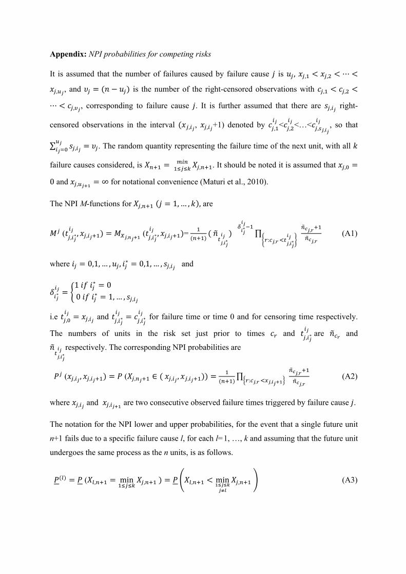
Appendix: NPI probabilities for competing risks

It is assumed that the number of failures caused by failure cause 𝑗 is 𝑢R, 𝑥R,' < 𝑥R,f < ⋯ <

𝑥R,nV, and 𝜐R = (𝑛 − 𝑢R) is the number of the right-censored observations with 𝑐R,' < 𝑐R,f <

⋯ < 𝑐R,pV, corresponding to failure cause 𝑗. It is further assumed that there are 𝑠R,.V right-

censored observations in the interval (𝑥R,.V, 𝑥R,.V+1) denoted by 𝑐R,'.V <𝑐R,f

.V <…<𝑐R,\V,DV.V , so that

∑ 𝑠R,.VnV.VrL

= 𝜐R. The random quantity representing the failure time of the next unit, with all 𝑘

failure causes considered, is 𝑋#*' = t.#'QRQG 𝑋R,#*'. It should be noted it is assumed that 𝑥R,L =

0 and 𝑥R,nV89 = ∞ for notational convenience (Maturi et al., 2010).

The NPI M-functions for 𝑋R,#*' (𝑗 = 1,… , 𝑘), are

𝑀R (𝑡R,.V∗.V , 𝑥R,.V*') = 𝑀6V,7V89

(𝑡R,.V∗.V , 𝑥R,.V*')=

'(#*')

(𝑛;cV,DV∗

DV )wDV∗DV/'

∏#;<V,=*'

#;<V,=x?:AV,=BcV,DV∗

DV y (A1)

where 𝑖R = 0,1, … , 𝑢R, 𝑖R∗ = 0,1, … , 𝑠R,.V and

𝛿.V∗.V = x

1𝑖𝑓𝑖R∗ = 00𝑖𝑓𝑖R∗ = 1,… , 𝑠R,.V

i.e 𝑡R,L.V = 𝑥R,.V and 𝑡R,.V∗

.V = 𝑐R,.V∗.V for failure time or time 0 and for censoring time respectively.

The numbers of units in the risk set just prior to times 𝑐? and 𝑡R,.V∗.V are 𝑛;A= and

𝑛;cV,DV∗

DV respectively. The corresponding NPI probabilities are

𝑃R (𝑥R,.V , 𝑥R,.V*') = 𝑃 (𝑋R,#V*' ∈ (𝑥R,.V , 𝑥R,.V*')) ='

(#*')∏

#;<V,=*'

#;<V,=|?:AV,=BCV,DV89} (A2)

where 𝑥R,.V and 𝑥R,.V89 are two consecutive observed failure times triggered by failure cause𝑗.

The notation for the NPI lower and upper probabilities, for the event that a single future unit

n+1 fails due to a specific failure cause l, for each l=1, …, k and assuming that the future unit

undergoes the same process as the n units, is as follows.

𝑃(M) = 𝑃 (𝑋M,#*' = min'QRQG

𝑋R,#*') = 𝑃 S𝑋M,#*' < min9UVUHVWX

𝑋R,#*'Y (A3)

𝑃(M)= 𝑃 (𝑋M,#*' = min

'QRQG𝑋R,#*') = 𝑃 S𝑋M,#*' < min

9UVUHVWX

𝑋R,#*'Y (A4)

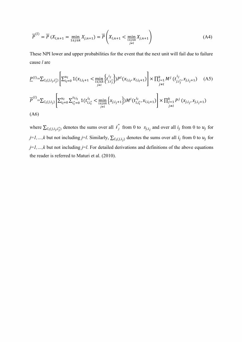
These NPI lower and upper probabilities for the event that the next unit will fail due to failure

cause l are

𝑃(M)=∑ ~∑ 1(𝑥M,.X*' <nX.XrL min

9UVUHVWX

�𝑡R,.V∗.V �)𝑃M(𝑥M,.X , 𝑥M,.X*')�gX(R,.V,.V

∗) × ∏ 𝑀RGRr'R�M

(𝑡R,.V∗.V , 𝑥R,.V*') (A5)

𝑃(M)

=∑ ~∑ ∑ 1(𝑡M,.X∗.X <

\X,DX.X∗rL

nX.XrL min

9UVUHVWX

|𝑥R,.V*'})𝑀M(𝑡M,.X∗

.X , 𝑥M,.X*')�gX(R,.V) × ∏ 𝑃RGRr'R�M

(𝑥R,.V , 𝑥R,.V*')

(A6)

where ∑gX(R,.V,.V∗) denotes the sums over all from 0 to 𝑠R,.V and over all 𝑖R from 0 to 𝑢R for

j=1,…,k but not including j=l. Similarly, ∑gX(R,.V) denotes the sums over all 𝑖R from 0 to 𝑢R for

j=1,…,k but not including j=l. For detailed derivations and definitions of the above equations

the reader is referred to Maturi et al. (2010).

*ji

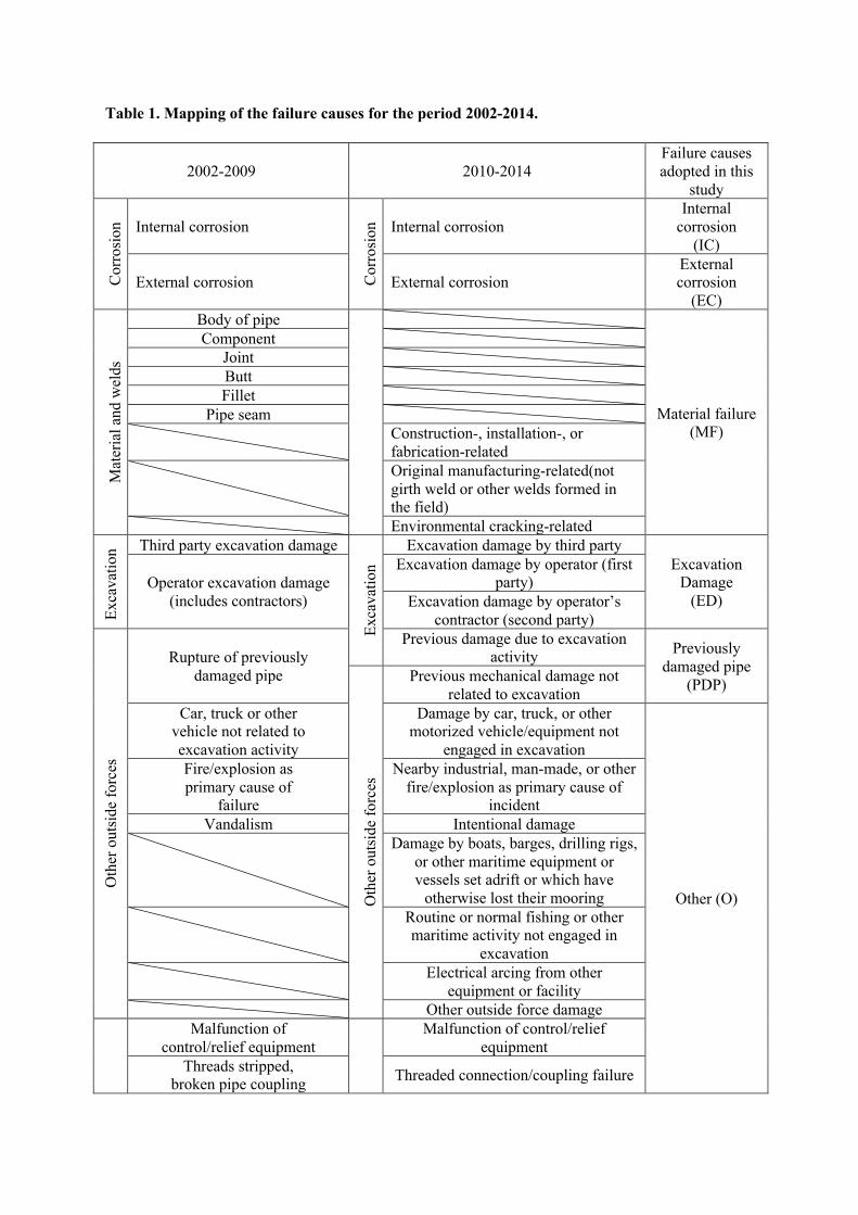
Table 1. Mapping of the failure causes for the period 2002-2014.

2002-2009 2010-2014 Failure causes adopted in this

study

Cor

rosi

on Internal corrosion

Cor

rosi

on Internal corrosion

Internal corrosion

(IC)

External corrosion External corrosion External corrosion

(EC)

Mat

eria

l and

wel

ds

Body of pipe

Material failure (MF)

Component Joint Butt Fillet

Pipe seam Construction-, installation-, or

fabrication-related Original manufacturing-related(not

girth weld or other welds formed in the field)

Environmental cracking-related

Exca

vatio

n Third party excavation damage

Exca

vatio

n

Excavation damage by third party Excavation

Damage (ED)

Operator excavation damage (includes contractors)

Excavation damage by operator (first party)

Excavation damage by operator’s contractor (second party)

Oth

er o

utsi

de fo

rces

Rupture of previously damaged pipe

Previous damage due to excavation activity Previously

damaged pipe (PDP)

Oth

er o

utsi

de fo

rces

Previous mechanical damage not related to excavation

Car, truck or other vehicle not related to excavation activity

Damage by car, truck, or other motorized vehicle/equipment not

engaged in excavation

Other (O)

Fire/explosion as primary cause of

failure

Nearby industrial, man-made, or other fire/explosion as primary cause of

incident Vandalism Intentional damage

Damage by boats, barges, drilling rigs, or other maritime equipment or vessels set adrift or which have

otherwise lost their mooring

Routine or normal fishing or other maritime activity not engaged in

excavation

Electrical arcing from other equipment or facility

Other outside force damage Malfunction of

control/relief equipment Malfunction of control/relief

equipment Threads stripped,

broken pipe coupling Threaded connection/coupling failure

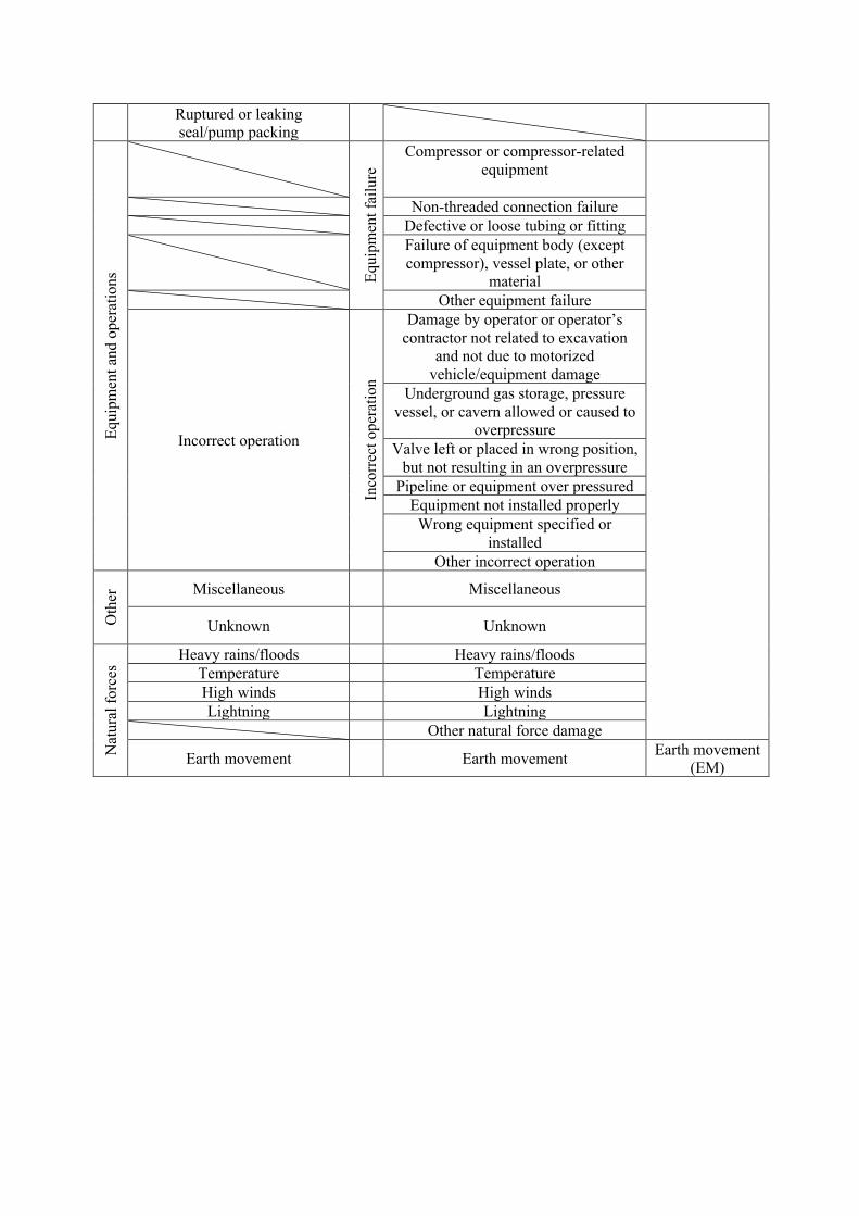
Ruptured or leaking seal/pump packing

Eq

uipm

ent a

nd o

pera

tions

Equi

pmen

t fai

lure

Compressor or compressor-related equipment

Non-threaded connection failure Defective or loose tubing or fitting Failure of equipment body (except

compressor), vessel plate, or other material

Other equipment failure

Incorrect operation

Inco

rrec

t ope

ratio

n

Damage by operator or operator’s contractor not related to excavation

and not due to motorized vehicle/equipment damage

Underground gas storage, pressure vessel, or cavern allowed or caused to

overpressure Valve left or placed in wrong position,

but not resulting in an overpressure Pipeline or equipment over pressured

Equipment not installed properly Wrong equipment specified or

installed Other incorrect operation

Oth

er Miscellaneous Miscellaneous

Unknown Unknown

Nat

ural

forc

es Heavy rains/floods Heavy rains/floods

Temperature Temperature High winds High winds Lightning Lightning

Other natural force damage

Earth movement Earth movement Earth movement (EM)

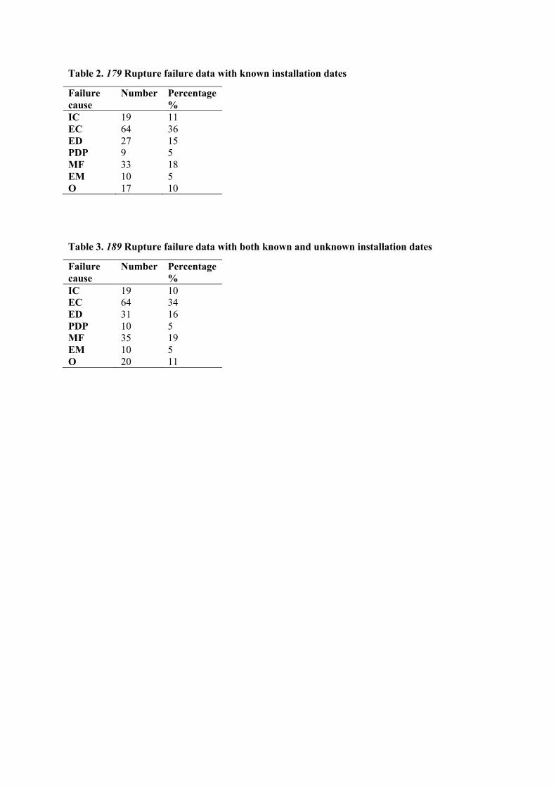
Table 2. 179 Rupture failure data with known installation dates

Failure cause

Number Percentage %

IC 19 11 EC 64 36 ED 27 15 PDP 9 5 MF 33 18 EM 10 5 O 17 10

Table 3. 189 Rupture failure data with both known and unknown installation dates

Failure cause

Number Percentage %

IC 19 10 EC 64 34 ED 31 16 PDP 10 5 MF 35 19 EM 10 5 O 20 11

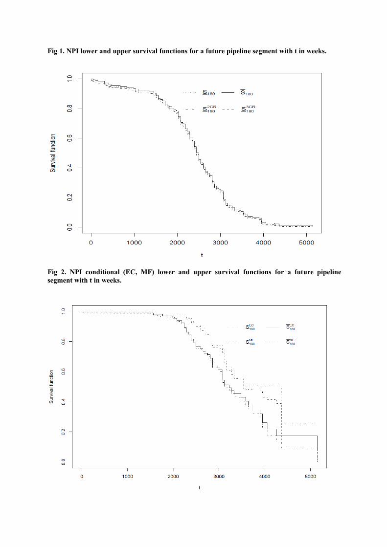
Fig 1. NPI lower and upper survival functions for a future pipeline segment with t in weeks.

Fig 2. NPI conditional (EC, MF) lower and upper survival functions for a future pipeline segment with t in weeks.

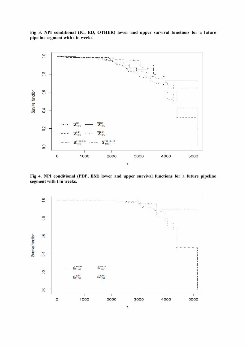
Fig 3. NPI conditional (IC, ED, OTHER) lower and upper survival functions for a future pipeline segment with t in weeks.

Fig 4. NPI conditional (PDP, EM) lower and upper survival functions for a future pipeline segment with t in weeks.