Competing Manufacturers in a Retail Supply Chain: OnContractual Form and Coordination1

Gérard P. Cachon A. Gürhan KökThe Wharton School Fuqua School of Business

University of Pennsylvania Duke UniversityPhiladelphia PA, 19104 Durham NC, 27708

cachon@wharton.upenn.edu gurhan.kok@duke.eduopim.wharton.upenn.edu/~cachon faculty.fuqua.duke.edu/~agkok

November 25, 2007

Abstract

It is common for a retailer to sell products from competing manufacturers. How then should the�rms manage their contract negotiations? The supply chain coordination literature focuses eitheron a single manufacturer selling to a single retailer or one manufacturer selling to many (possiblycompeting) retailers. We �nd that some key conclusions from those market structures do not applyin our setting. We allow the manufacturers to compete for the retailer�s business using one ofthree types of contracts, a wholesale-price contract, a quantity-discount contract or a two-parttari¤. It is well known that there are two reasons why a monopolist manufacturer prefers either ofthe latter two, more sophisticated, contracts relative to the wholesale-price contract. First, theycan be used to coordinate the supply chain, meaning that they induce the retailer to sell morebecause they reduce the double marginalization caused by wholesale-price contracts. Second, theycan be used to extract rents from the retailer, in theory allowing the manufacturer to leave theretailer only with her reservation pro�t. However, we show that in our market structure these twosophisticated contracts force the manufacturers to compete more aggressively than when they onlyo¤er wholesale-price contracts, and this may leave them worse o¤ and the retailer substantiallybetter o¤. In other words, although in a serial supply chain a retailer may have just cause tofear quantity discounts and two-part tari¤s, a retailer may actually prefer those contracts wheno¤ered by competing manufacturers. We conclude that the properties a contractual form exhibitsin a one-manufacturer supply chain may not carry over to the realistic setting in which multiplemanufacturers must compete to sell their goods through a single retailer.

1The authors would like to thank Awi Federgruen and Richard Staelin for helpful discussions.

1. Introduction

The literature on supply chain coordination has studied several contractual forms in settings with

a single manufacturer and one or more retailers. One of the key results from this literature

is that wholesale-price contracts lead to suboptimal decisions for the supply chain (i.e., double

marginalization) and more sophisticated contracts (like quantity discounts or two-part tari¤s) can

be employed to achieve both channel coordination (i.e., maximize the supply chain�s pro�t) and

rent extraction (i.e., the ability to allocate a high share of the pro�ts to the manufacturer). Our

objective in this paper is to test this conclusion in a setting in which multiple manufacturers

compete to sell their products through a single retailer.

In our model, two manufacturers simultaneously o¤er to the retailer one of three types of

contracts: a wholesale-price contract, a quantity-discount contract (i.e., a decreasing per-unit price

in the quantity purchased) or a two-part tari¤ (i.e., a per unit price and a �xed fee). The retailer�s

prices determine the products�demand rates, and she sets her prices to maximize her total pro�t

given the o¤ered contracts and her inventory costs, which may exhibit economies of scale.

As with all supply chain structures, the �rms are indirectly interested in the total pro�t in

the supply chain, and more directly interested in their share of that pro�t. In supply chains

with a monopolist manufacturer it has been shown that a properly designed quantity-discount or

two-part tari¤ allows the manufacturer to maximize his product�s total pro�t (i.e., the two �rms�

combined pro�t). Furthermore, the manufacturer can extract the largest possible share of that

pro�t, thereby leaving the retailer with her reservation pro�t, which is the pro�t the retailer can

earn if the retailer rejects the contract. In a serial supply chain the retailer�s reservation pro�t is

assumed to be an exogenous constant that re�ects the retailer�s bargaining power - an increase in

the retailer�s bargaining power is modeled by increasing the retailer�s reservation pro�t. However,

in our structure with two manufacturers, the retailer�s reservation pro�t is endogenous - the pro�t

the retailer can earn if it were to reject manufacturer A�s o¤er depends on what manufacturer B

o¤ers, and vice-versa. This distinction is signi�cant and, as we demonstrate, important for our

�ndings.

We show that, holding the other manufacturer�s contract o¤er �xed, a manufacturer can increase

its pro�t by using a more sophisticated contract relative to a wholesale-price contract. Furthermore,

1

in equilibrium (i.e., a pair of contracts such that neither manufacturer has an incentive to o¤er a dif-

ferent contract given the other manufacturer�s contract o¤er), we show that the more sophisticated

contracts can increase the supply chain�s total pro�t, again relative to the wholesale-price contract.

These results are analogous to those found in models with a monopolist manufacturer. However,

in sharp contrast to the results with one manufacturer, we also �nd that in equilibrium, if the

products are close substitutes, the manufacturers may earn substantially less when sophisticated

contracts are o¤ered and the retailer may earn substantially more.

In a one-manufacturer setting sophisticated contracts are advantageous to the manufacturer

because they allow the manufacturer to increase and extract rents. These abilities are present

even with multiple manufacturers (holding the other manufacturer�s contract �xed), but now there

is an additional e¤ect - the sophisticated contracts also yield more aggressive competition between

the manufacturers. This additional e¤ect may dominate the others - quantity discounts and two-

part tari¤s e¤ectively increase the retailer�s bargaining power relative to wholesale price contracts,

so much so that the manufacturers can be worse o¤ with them relative to an equilibrium in which

they both o¤er wholesale-price contracts. To explain further, in our multiple-manufacturer model

the retailer�s reservation pro�t is endogenous and competition between the manufacturers serves to

raise it, in particular when sophisticated contracts are used.

The rest of the paper is organized as follows. Section 2 reviews the relevant literature. Section

3 describes the model. Section 4 present our analysis of the retailer�s problem, Section 5 the

analysis of the wholesale and quantity-discount games, and Section 6 the analysis of two-part tari¤

games. Section 7 concludes the paper. All proofs are presented in Appendix A.

2. Literature Review

The present paper is foremost a commentary on the supply chain coordination literature (see

Cachon 2003 for a review). As already discussed, this literature focuses on either relationships

with bilateral monopoly or models with one manufacturer and multiple retailers. Wholesale-price

contracts are nearly always found to be ine¢ cient and more sophisticated contracts can be used

to eliminate that ine¢ ciency and reallocate rents arbitrarily between the parties in the supply

2

chain.2 Choi (1991), Trivedi (1998), Lee and Staelin (1997), and Martinez de Albeniz and Roels

(2007) do study systems with multiple manufacturers and a common retailer, but they only consider

wholesale-price contracts.

There is an extensive literature on supply chain coordination with quantity-discount contracts

(e.g., Jeuland and Shugan 1983, Moorthy 1987, Ingene and Perry 1995) but they consider only

one manufacturer. There is also a considerable literature in operation management on lot-size

coordination with �xed demand (e.g., Monahan 1984, Corbett and de Groote 2000). We also

consider operational issues, but our retailer can adjust demand via her prices. Two-part tari¤s

are studied by Bernheim and Whinston (1998), O�Brien and Sha¤er (1997), and Mathewson and

Winter (2001) in models with multiple manufacturers and a single retailer. They explore whether

or not the exclusion of a manufacturer occurs and the implications for anti-trust laws. They do

not consider the wholesale or quantity-discount contracts and the pro�t level of individual �rms.

Related to two-part tari¤s, there is a literature on slotting fees (which are essentially two-part tari¤s

with negative payments to the manufacturer, see, for example, Marx and Sha¤er 2004). Kuksov

and Pazgal (2007) show that slotting fees do not occur in a setting with simultaneous manufacturer

competition and a single retailer, and the same result applies in our model.

McGuire and Staelin (1983) study two competing supply chains under two structural forms:

in each supply chain either the manufacturer sells to a dedicated retailer via a wholesale-price

contract or the manufacturer vertically integrates into retailing. In either structure the products

of the two manufacturers are sold to consumers from di¤erent �rms, whereas in our model the

manufacturers� products are sold through a single independent retailer. Nevertheless, there are

some similarities in our results. McGuire and Staelin (1983) �nd that the manufacturers may

prefer to sell via wholesale-price contracts, despite the fact that they do not coordinate the channel

nor allow the manufacturer to extract all rents, because they dampen retail competition between

the two products relative to the vertically integrated structure. In our model, competition to

consumers is held constant, because we have a single retailer, so what changes is the retailer�s

bargaining power relative to the manufacturers.

2A wholesale-price contract can maximize pro�ts in a system with one manufacturer and multiple quantity com-peting retailers. However, it provides only one allocation of the system�s rents and it isn�t even the manufacturer�soptimal wholesale price (see Cachon and Lariviere 2005). If retailers compete on price and quantity, then the wholesaleprice no longer guarantees coordination (see Bernstein and Federgruen 2003, 2005).

3

3. The Model

There are two products in the market supplied by two di¤erent manufacturers. The products are

partial substitutes and are sold through a common retailer. In the �rst stage of the game, the

manufacturers simultaneously announce the payment schemes for their products. In the second

stage, the retailer chooses prices, which determine the products�demand rates, to maximize her

pro�t. In addition to the payments to the manufacturer, the retailer incurs operating costs that

depend on the average volume sold of each product. The manufacturers incur constant marginal

production costs.

The retailer faces price sensitive customers. The revenue from product i is

Ri(d) = pi(d)di;

where di is the demand rate of product i; d is the pair of demand rates, and the inverse demand

function is

pi(d) = �i � �idi � idj ; and �i > j > 0 for all i; j:

We elect to work with the inverse demand function for expositional simplicity. The formulation

with the demand function is equivalent to the above.

Let Gi(di) be the retailer�s inventory related operational costs of product i,

Gi(di) = Kid�i ; Ki � 0, 0 < � < 1;

where Ki and � are exogenous constants. This functional form, which exhibits economies of scale,

is a general representation of the inventory costs that arise in common inventory replenishment

models such as a base-stock model3 or an economic order quantity model4.

Let �i denote the retailer�s pro�t from product i and � = �i + �j , the retailer�s total pro�t. It

follows that

�i = Ri(d)�Gi (di)� Ti (di) ;3 In a periodic review model where demand follows a Normal distribution with mean di and standard deviation

�id�i , the total inventory related costs with the optimal base-stock level is given by (b+ h)�(z

�)�id�i ; where b is the

backlog penalty per unit, and h is the inventory holding cost per period. De�ning Ki = (b+ h)�(z�)�i leads to the

Gi function.4 In the economic order quantity (EOQ) model, the retailer incurs a �xed cost ki per order and a holding cost hi

per unit of inventory held for one period. The well known EOQ formula suggests ordering everyp2ki=hidi periods.

The resulting optimal inventory and ordering costs is given byp2kidihi: De�ning Ki =

p2kihi leads to the Gi

function with � = 1=2.

4

and Ti(di) is the payment made to the manufacturer based on the retailer�s demand rate and their

agreed upon contract.5 Manufacturer i�s pro�t is

�i = Ti(di)� cidi; (1)

where ci is the manufacturer�s cost per unit.

We consider three di¤erent types of contracts. With a wholesale-price contract, the payment

function is

Ti(di) = widi;

where wi is the wholesale price chosen by manufacturer i.

We include the following set of quantity-discount contracts:

Ti(di) =

�widi � vid2i =2; if di � (wi � ci) =viTi((wi � ci) =vi) + ci (di � (wi � ci) =vi) ; otherwise.

(2)

where wi is a �exible parameter chosen by the manufacturer, ci is the manufacturer�s marginal

cost per unit, and vi is an exogenous constant, where vi 2 [0; �v); �v = 2�i �� i + j

�: We have

intentionally designed this set of quantity-discount contracts such that (1) they have a single para-

meter, just like the wholesale-price contract, wi, and (2) wholesale-price contracts are a subset of

our quantity-discount contracts - a quantity discount with vi = 0 is a wholesale-price contract.

Although we only consider a subset of possible quantity discounts, this is not overly restrictive.

Our quantity discounts are continuous, di¤erentiable, concave, and the manufacturer does not

sell even the marginal unit for less than its production cost. The bound on vi implies that the

quantity-discount is not too �aggressive� in the sense that the marginal price paid does not fall

too rapidly as the purchase volume increases, i.e., T 00i (di) � �vi: In fact, it can be shown that

our quantity-discounts are optimal for the manufacturer (holding the other manufacturer�s contract

o¤er �xed) given the T 00i (di) � �vi constraint and assuming di¤erentiability (see Proposition 2 in

Appendix A). Furthermore, T 00i (di) � �vi ensures the retailer�s pro�t function minus operational

costs is strictly concave in (d1; d2) : This naturally raises the question of whether the manufacturer

could do better by o¤ering an even more aggressive quantity discount. The manufacturer can

5The retailer�s payment Ti(di) to a manufacturer can be interpreted as a yearly (average) payment based on yearly(average) volume. Many manufacturer-retailer purchasing contracts are based on the yearly volume rather than onthe volume of individual shipments.

5

do better, but we have found that an equilibrium in the manufacturer�s contract o¤er game may

not exist when we consider more aggressive quantity discounts. However, a two-part tari¤ can be

interpreted as the most aggressive quantity discount, and we do have results for those contracts.

Thus, although we cannot characterize the equilibrium dynamics for all quantity discounts, we have

results for quantity-discounts that are more aggressive than wholesale-price contracts and results

for the most aggressive contract, the two-part tari¤.

As already mentioned, our third contract form is the two-part tari¤, which is characterized by

a �xed fee Fi and a marginal cost wi :

Ti (di) = Fi1fdi>0g + widi; (3)

where indicator function 1fdi>0g = f1; if di > 0; 0; otherwiseg.

A symmetric game across manufacturers means that the data for the two products are identical,

i.e., ci, �i; �i, i; Ki; vi are the same for any i: The subscript i will be dropped in those cases. In

a symmetric solution, the decisions (di at the retail level, wi or Ti at the manufacturer level) are

identical across products.

In the following sections, we solve the problem using backward induction. We analyze the

retailer�s decision �rst and then the game between the manufacturers.

4. The Retailer�s Problem

In the �rst stage of the game, the manufacturers simultaneously announce their contract o¤ers. We

assume that the particular contractual form o¤ered is established before the game begins, but we

later discuss what happens when the manufacturers choose their contractual form and parameters

simultaneously. In the second stage, given functions T1 and T2; the retailer chooses the demand

rates to maximize her pro�t.

4.1 The retailer�s decision with quantity discounts

In this section we assume the manufacturers o¤er the retailer quantity discounts, which, as discussed

earlier, are wholesale-price contracts when vi = 0: We defer the discussion of two-part tari¤s to

Section 6.

6

De�ne

di(dj) = argmaxdif�i(di; dj)g; (4)

( ~di; ~dj) = argmaxdi;dj

f�(di; dj) : didj > 0g ; (5)

~� = �( ~di; ~dj) (6)

The retailer�s optimization problem can now be written as

maxf~�; �1(d1(0); 0); �2(0; d2(0))g: (7)

Hence, the optimal solution to the retailer�s problem is

(d�1; d�2) 2 f( ~d1; ~d2); (d1(0); 0); (0; d2(0))g:

For expositional simplicity, we assume the retailer breaks ties in favor of carrying a full product

line, if possible, over a single product.

Consider the problem of maximizing total supply chain pro�t. It is equivalent to the retailer�s

problem if the manufacturers charge only their production cost. De�ne �̂1 = �1(d1(0); 0); �̂2 =

�2(0; d2(0)); and �̂12 = �( ~d1; ~d2) when Ti(di) = cidi for i = 1; 2. These pro�t levels are respectively

the maximum pro�t the system earns, if it were to carry only product 1, only product 2 and both

products. We assume

�̂12 > �̂i > 0; for i = 1; 2; (8)

which implies that it is always optimal for the system to carry both products.

Now return to the system with independent manufacturers and a retailer. Let Hi denote the

�rst derivative of � with respect to di. We have

Hi = @�=@di = �i � 2�idi �� i + j

�dj �G0i (di)� T 0i (di) ; j 6= i: (9)

Consider �rst the case with no economies of scale (i.e., K1 = K2 = 0). The retailer�s pro�t function

� is jointly concave in (d1; d2) ; so the unique solution to fHi = 0; i = 1; 2g is the unique optimal

solution. If an interior solution does not exist, then the optimal solution is either (d1(0); 0) or

(0; d2(0)); where di(0) is the unique solution to Hi = 0 with dj = 0: Because � is well behaved, the

optimal solution (d�1; d�2) can be easily characterized and it is a continuous, di¤erentiable function

of the problem inputs such as the parameters of the manufacturer contracts.

7

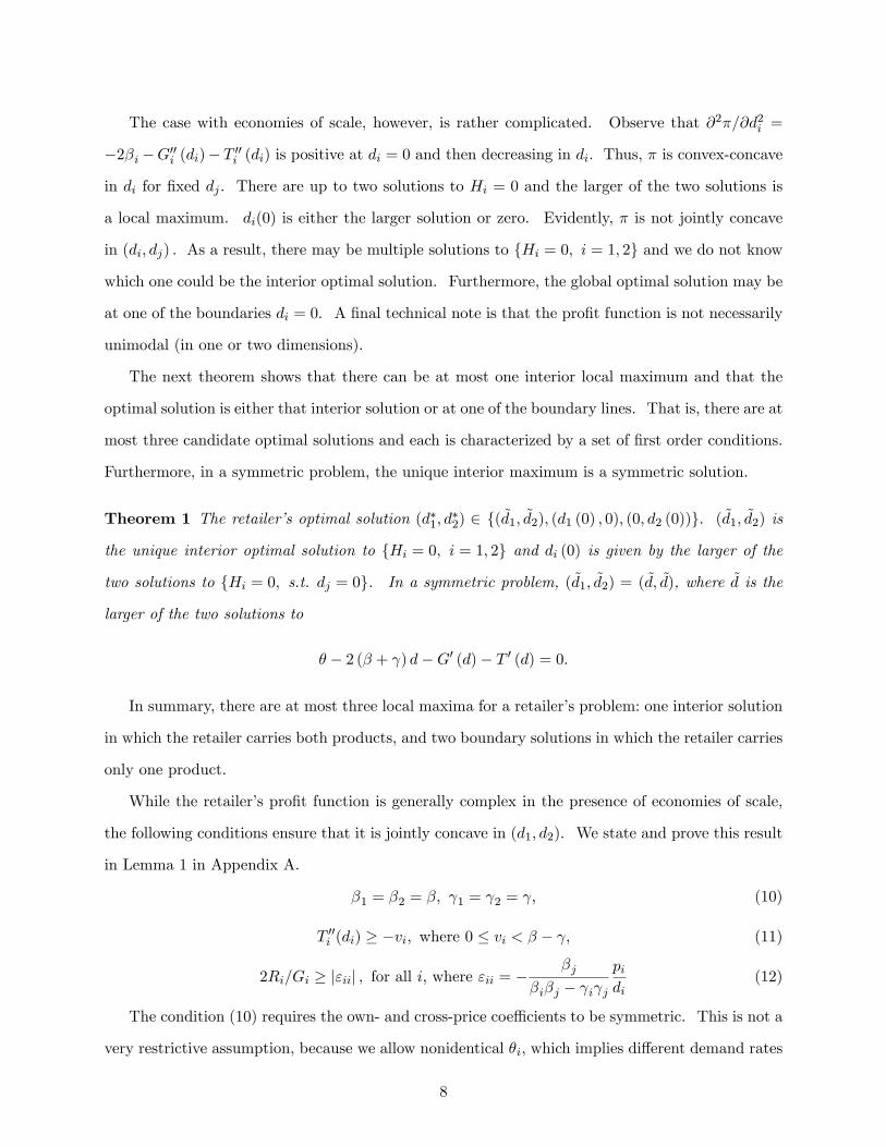
The case with economies of scale, however, is rather complicated. Observe that @2�=@d2i =

�2�i�G00i (di)� T 00i (di) is positive at di = 0 and then decreasing in di: Thus, � is convex-concave

in di for �xed dj : There are up to two solutions to Hi = 0 and the larger of the two solutions is

a local maximum. di(0) is either the larger solution or zero. Evidently, � is not jointly concave

in (di; dj) : As a result, there may be multiple solutions to fHi = 0; i = 1; 2g and we do not know

which one could be the interior optimal solution. Furthermore, the global optimal solution may be

at one of the boundaries di = 0. A �nal technical note is that the pro�t function is not necessarily

unimodal (in one or two dimensions).

The next theorem shows that there can be at most one interior local maximum and that the

optimal solution is either that interior solution or at one of the boundary lines. That is, there are at

most three candidate optimal solutions and each is characterized by a set of �rst order conditions.

Furthermore, in a symmetric problem, the unique interior maximum is a symmetric solution.

Theorem 1 The retailer�s optimal solution (d�1; d�2) 2 f( ~d1; ~d2); (d1 (0) ; 0); (0; d2 (0))g: ( ~d1; ~d2) is

the unique interior optimal solution to fHi = 0; i = 1; 2g and di (0) is given by the larger of the

two solutions to fHi = 0; s.t. dj = 0g. In a symmetric problem, ( ~d1; ~d2) = ( ~d; ~d), where ~d is the

larger of the two solutions to

� � 2 (� + ) d�G0 (d)� T 0 (d) = 0:

In summary, there are at most three local maxima for a retailer�s problem: one interior solution

in which the retailer carries both products, and two boundary solutions in which the retailer carries

only one product.

While the retailer�s pro�t function is generally complex in the presence of economies of scale,

the following conditions ensure that it is jointly concave in (d1; d2). We state and prove this result

in Lemma 1 in Appendix A.

�1 = �2 = �; 1 = 2 = ; (10)

T 00i (di) � �vi; where 0 � vi < � � ; (11)

2Ri=Gi � j"iij ; for all i, where "ii = ��j

�i�j � i jpidi

(12)

The condition (10) requires the own- and cross-price coe¢ cients to be symmetric. This is not a

very restrictive assumption, because we allow nonidentical �i; which implies di¤erent demand rates

8

and price elasticities for the products. The condition (11) is stricter than our earlier assumption: it

requires the quantity discount to be less concave to guarantee the concavity of the retailer�s pro�t

function. The condition (12) stipulates that the own-price elasticity ("ii) is less than two times the

revenues-to-average inventory costs ratio of the product. (It is similar to the conditions Bernstein

and Federgruen (2003) developed for decentralized retailers.)

5. Manufacturers�Problem

In this section, we analyze the game between the manufacturers assuming they o¤er quantity

discounts (possibly with vi = 0): In the presence of economies of scale (i.e., Ki > 0 for any i),

we assume that conditions (10)-(11) hold and we restrict our attention to a region de�ned by (12).

Each manufacturer chooses its own best response Ti(Tj) given the other manufacturer�s contract

Tj .

Ti(Tj) = argmaxTi(d)

�i(d�) for all i; where d� = argmax�: (13)

An equilibrium of the game is a pair of contracts (T �i ; T�j ) such that neither manufacturer has an

incentive to o¤er a di¤erent contract.

The following remark demonstrates how the contracting problem with multiple manufacturers

is di¤erent from that with a single manufacturer.

Remark 1 For any �xed contract o¤ered by manufacturer 2 such that �2(0; d2(0)) > 0 :

1. Consider the set of contracts such that the retailer�s payment to manufacturer 1 is a non-

decreasing function of d1: There does not exist a contract in this set such that the manufac-

turer can extract all of the pro�t from his product (i.e., it is not possible to have �1 > 0 and

�1 = 0).

2. The retailer accepts manufacturer 1�s contract o¤er and stocks both products only if

�1( ~di; ~dj) � �2(0; d2(0))� �2( ~di; ~dj) (14)

Unlike in a serial supply chain, the �rst statement implies that a manufacturer must leave the

retailer with some pro�t to induce the retailer to carry the manufacturer�s product (see Appendix

A for a detailed proof). In other words, the retailer�s reservation pro�t for carrying a product is

9

greater than zero. However, this does not mean that a single reservation pro�t exists. The second

statement provides an intuitive condition, (14), for when the retailer is willing to carry manufacturer

1�s product - the retailer must earn more with product 1 in the assortment than without product

1 in the assortment. The right hand side of (14) can be considered the retailer�s reservation

pro�t that the retailer must earn from product 1 for the retailer to be willing to carry product 1.

The �rst term, �2(0; d2(0)); is �xed, given manufacturer 2�s contract o¤er. However, the second

term, �2( ~di; ~dj); depends on manufacturer 1�s contract o¤er (assuming the mild condition that the

optimal interior demands, ( ~di; ~dj); change smoothly in the contract parameters). Therefore, even

if manufacturer 2�s contract o¤er is held �xed, there does not exist a reservation pro�t for product

1 that is independent of manufacturer 1�s contract o¤er, as is assumed in models with a single

manufacturer. Put another way, a serial supply chain with a �xed reservation pro�t for the retailer

cannot replicate the dynamics of our model.

It remains to characterize the equilibrium contract o¤ers by the manufacturers. We are able to

partially characterize the equilibrium of the contract o¤er game when the products are symmetric

(i.e., identical �i; �i; i; ci;Ki; vi). We start with the following observation that rules out equilibria

in which the retailer carries only one product.

Remark 2 In a symmetric game, there does not exist a manufacturer equilibrium where di = 0

for some i:

The result is due to (8), which guarantees that the inclusion of a manufacturer strictly increases

system pro�t. Suppose there were an equilibrium in which manufacturer i is excluded. Regardless

of the fraction of �̂j the retailer earns, manufacturer i can o¤er to sell to the retailer at ci + " for

an arbitrarily small " and then the retailer�s pro�t increases if it carries product i: If j is excluded

as a result, it will react similarly and be included.

De�ne w¯ i(wj) = maxfwi : d�j (wi; wj) = 0g, the maximum wi that makes the retailer exclude

product j; �wi (wj) = minfwi : d�i (wi; wj) = 0g, the minimum wholesale price of i that makes

the retailer exclude product i: Note that w¯ i(wj) may not exist for every wj : In that case, set

w¯ i(wj) = ci: De�ne wi (wj) as the best response of manufacturer i, which can be found via a

line-search between [w¯ i; �wi] :

The following theorem characterizes the unique symmetric equilibrium of the contract o¤er

10

game.

Theorem 2 Consider a symmetric game in which the manufacturers o¤er quantity discounts.

There exists a unique solution to

d�i (w1; w2) + (wi � vi � ci)@d�i@wi

= 0; for all i;

denoted (w�1; w�2); which is the unique candidate to be a symmetric equilibrium.

As can be seen in the proof of the above theorem, showing the unimodality of a manufacturer�s

pro�t in wi requires the use of the second-order properties of the retailer�s optimal solution (d�1; d�2) :

The analysis of a manufacturer game that depends on the solution of a complex problem at the

retailer presents technical di¢ culties in the presence of economies of scale, that have not been

present in any other competition paper in the literature.

We cannot guarantee that the candidate point described in Theorem 2 is an equilibrium. We

show that at (w�1; w�2) ; w

�i is a local optimum for manufacturer i, and �i is concave for wi >

w�i : However, the optimal solution wi(w�j ) may be di¤erent than w�i in the range [w¯ i

; w�i ] : If

wi(w�j ) = w

�i ; then (w

�1; w

�2) is indeed an equilibrium point. If not, there there exists no symmetric

equilibrium.

Now consider the situation in which there are no economies of scale. This substantially sim-

pli�es the analysis of both the retailer�s demand decisions and the manufacturers�contract o¤er

problem. For any (v1; v2) and asymmetric products, we can now guarantee joint concavity of the

retailer�s pro�t and the existence and the uniqueness of the equilibrium without the symmetry

assumptions. The next theorem provides the closed form solutions for the demand rates and the

contract parameters by solving the �rst-order conditions given in Theorem 2 for the general case.

Theorem 3 With no economies of scale (i.e., Ki = 0); there exists a unique equilibrium of the

game in which the manufacturers o¤er quantity discounts. It is characterized by the following

reaction functions and the optimal demand rates:

d�i =

�2�j � vj

�(�i � wi)�

� i + j

�(�j � wj)

(2�i � vi)�2�j � vj

��� i + j

�2 ;

wi(wj) =

��2�j � vj

�(�i)�

� i + j

�(�j � wj)

� �� + vi

�2�j � vj

��+ ci

�2�j � vj

���

2�j � vj� �� + � + vi

�2�j � vj

�� ;

where � � (2�i � vi)�2�j � vj

��� i + j

�2:

11

In this section we have assumed that the manufacturers o¤er quantity discounts with an exoge-

nously speci�ed vi: Suppose the manufacturers now simultaneously o¤er a (wi; vi) where they are

free to choose any vi 2 [0; v). In other words, they can choose to o¤er a wholesale-price contract

(vi = 0) or a quantity discount (vi > 0): The next proposition indicates, as in supply chains with

a single manufacturer, that a manufacturer prefers to o¤er a quantity-discount contract and, in

particular, prefers more aggressive quantity discounts. Quantity discounts allow the manufacturer

to increase supply chain rents (i.e., reduce double marginalization) and to extract rents, so they are

the preferred contract when the other manufacturer�s contract is held �xed even when the retailer

can adjust its demand allocations between the two products in response.

Proposition 1 Manufacturer i�s pro�t strictly increases with vi at the optimal wi. That is, if a

manufacturer is given the option to choose between three contractual forms with vi 2 f0; a; bg such

that 0 < a < b; then �i(w�i jvi = 0) < �i(w�i jvi = a) < �i(w�i jvi = b):

5.1 Comparison of the Equilibrium underWholesale Price and Quantity-DiscountContracts

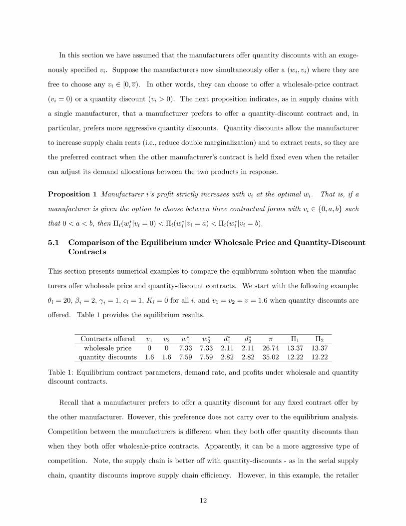
This section presents numerical examples to compare the equilibrium solution when the manufac-

turers o¤er wholesale price and quantity-discount contracts. We start with the following example:

�i = 20, �i = 2, i = 1, ci = 1, Ki = 0 for all i; and v1 = v2 = v = 1:6 when quantity discounts are

o¤ered. Table 1 provides the equilibrium results.

Contracts o¤ered v1 v2 w�1 w�2 d�1 d�2 � �1 �2wholesale price 0 0 7.33 7.33 2.11 2.11 26.74 13.37 13.37quantity discounts 1.6 1.6 7.59 7.59 2.82 2.82 35.02 12.22 12.22

Table 1: Equilibrium contract parameters, demand rate, and pro�ts under wholesale and quantitydiscount contracts.

Recall that a manufacturer prefers to o¤er a quantity discount for any �xed contract o¤er by

the other manufacturer. However, this preference does not carry over to the equilibrium analysis.

Competition between the manufacturers is di¤erent when they both o¤er quantity discounts than

when they both o¤er wholesale-price contracts. Apparently, it can be a more aggressive type of

competition. Note, the supply chain is better o¤ with quantity-discounts - as in the serial supply

chain, quantity discounts improve supply chain e¢ ciency. However, in this example, the retailer

12

(a) (b)

­25%

­20%

­15%

­10%

­5%

0%

5%

10%

0 0.5 1 1.5 2

v

% C

hang

e in

 Man

ufac

ture

r Pr

ofits

­5%

­4%

­3%

­2%

­1%

0%

1%

2%

0.0 0.2 0.4 0.6 0.8 1.0

v

% C

hang

e in

 Man

ufac

ture

r Pr

ofits

β=2.0, γ=1.0

β=1.8, γ=1.0

β=2.0, γ=0.8

β=2.0, γ=1.1

Κ=0, γ=1.0

Κ=3, γ=1.1

Κ=0, γ=1.0

Κ=0, γ=1.1

Figure 1: The e¤ect of the concavity of quantity discount contracts on manufacturer pro�ts: %change in �1 at equilibrium as v increases. Base case: � = 20; � = 2; = 1; c = 1;K = 0:

captures all of the improved e¢ ciency and even more, leaving the manufacturers worse o¤. This

need not always be true, as we next demonstrate.

Figure 1(a) plots the change in the manufacturers� pro�t as v is modi�ed. In our example,

if we reduce v from 1.6 to 0.4, then the manufacturers are somewhat better o¤ o¤ering quantity

discounts than wholesale-price contracts - in this case the manufacturer competition has not been

intensi�ed substantially, allowing them to increase their pro�t. However, if the products become

more substitutable (lower � or higher ), then the manufacturers can be worse o¤ with quantity-

discounts no matter how weak the quantity discounts are (i.e., no matter how low v is). On the

other hand, with less substitutable products (lower ) the manufacturers bene�t from quantity

discounts at equilibrium. Figure 1(b) shows that including inventory costs can make the negative

e¤ects of competition with quantity discounts on the manufacturers�pro�ts more pronounced.

We constructed a numerical study to better understand the extent of these observations. We

chose parameters from the following sets, leading to 108 scenarios: � = f20; 40g; � = f1; 2; 4g;

= f0:25; 0:5; 0:75g��; c = f1; 3g; K = f0; 1; 3g : Evaluating each scenario with v = f0; 0:5; 0:95g�

(� � ) ; i.e., under wholesale-price and two di¤erent quantity discount contracts, leads to a total

324 instances. In nine of the 108 scenarios, we haven�t been able to �nd an equilibrium for at

least one of the contracts (including the wholesale-price contracts in �ve scenarios). Investigating

13

the best response functions in those cases reveals that the e¤ect of the economies of scale is very

strong at the retailer and the manufacturers cycle between undercutting prices to get the retailer

to exclude the other manufacturer and being undercut. In those cases, there does not exist

an asymmetric equilibrium either. We report the results for the 297 instances that produced a

symmetric equilibrium of the game. As a validity check, we compare the average cost per unit that

the retailer pays to the manufacturers, T �(d)=d; with the two types of contracts: the average cost

is 5% lower in the quantity discounts equilibrium than the wholesale prices when v = 0:5 (� � )

and 11% lower when v = 0:95 (� � ) ; which indicates that the quantity discounts in equilibrium

in these examples are modest.

Table 2 provides a summary of the comparison of pro�ts under the quantity-discount equilibrium

relative to the wholesale-price equilibrium. In all cases, the supply chain pro�t and the retailer�s

pro�t increase when quantity discounts are o¤ered. For low substitutability levels (i.e., = 0:25�),

the manufacturers�pro�ts increase with the quantity-discount contract. Furthermore, the manu-

facturers�pro�t increase is greater than the supply chain�s pro�t increase, which means that the

manufacturers are able to extract a higher share of the supply chain�s pro�t. With medium and

high substitutability levels, however, the manufacturers�equilibrium pro�ts are generally lower with

quantity discounts than with wholesale-price contracts, and the magnitude of the pro�t loss can be

substantial, especially with a more aggressive quantity discount (i.e., higher v). In those cases the

e¤ect of more aggressive competition among the manufacturers dominates the e¤ect of increased

supply chain pro�ts. Finally, the negative e¤ect of quantity discounts on the manufacturers�prof-

its becomes more pronounced with increased economies of scale. For instance, with = 0:5�

and v = 0:95 (� � ) ; both the percentage of cases in which the manufacturers are worse o¤ and

the average magnitude of the manufacturers�loss increase with k: In summary, the decisions for

the two products are more tightly linked if they are close substitutes or the level of economies of

scale is high. This increases the retailer�s endogenous reservation pro�t (the value of the option

to carry more of the competitor�s product) and e¤ectively the retailer�s power in its relation with

each manufacturer. Our results suggest the manufacturers are better o¤ employing the simple

wholesale-price contracts when dealing with a powerful retailer rather than the more sophisticated

quantity discounts.

14

= 0:25� �v = 0:5� (� � ) v = 0:95� (� � )

k = 0 k = 1 k = 3 k = 0 k = 1 k = 3

Average % gain in total pro�t 5.7 6.0 6.0 11.2 11.5 11.7Average % gain in the retailer�s pro�t 3.3 3.2 3.2 6.0 5.9 6.0% of cases manufacturers are better o¤ 100 100 100 100 100 100Average % gain in manufacturer pro�ts 7.3 7.8 7.7 14.6 15.2 15.2% of cases manufacturers are worse o¤ 0 0 0 0 0 0Average % loss in manufacturer pro�ts n/a n/a n/a n/a n/a n/a

= 0:5� �Average % gain in total pro�t 3.1 3.6 3.7 6.8 6.9 7.1

Average % gain in the retailer�s pro�t 6.0 6.6 7.1 13.8 14.7 15.8% of cases manufacturers are better o¤ 100 100 100 9 0 0Average % gain in manufacturer pro�ts 0.8 0.7 0.5 0.2 n/a n/a% of cases manufacturers are worse o¤ 0 0 0 91 100 100Average % loss in manufacturer pro�ts n/a n/a n/a -0.2 -0.6 -1.2

= 0:75� �Average % gain in total pro�t 1.4 1.5 1.4 2.6 2.7 2.6

Average % gain in the retailer�s pro�t 5.9 6.1 6.3 12.4 12.9 13.1% of cases manufacturers are better o¤ 0 0 0 0 0 0Average % gain in manufacturer pro�ts n/a n/a n/a n/a n/a n/a% of cases manufacturers are worse o¤ 100 100 100 100 100 100Average % loss in manufacturer pro�ts -7.5 -8.1 -8.6 -16.9 -18.5 -19.3

Table 2: Summary statistics on supply chain, retailer and manufacturer pro�ts in the quantity-discount equilibrium relative to the wholesale-price equilibrium.

15

6. Two-part Tari¤s

In this section, we consider the game between manufacturers that o¤er two-part tari¤ contracts

and compare it with the outcome of the wholesale price game. Several papers in the industrial

organization literature (e.g., Bernheim and Whinston, 1998) provide a characterization of the equi-

librium with two-part tari¤s. The next theorem generalizes this characterization to the case with

economies of scale at the retailer.

Theorem 4 Given any contract by manufacturer j; the optimal contract of manufacturer i is a

two-part tari¤ contract of the type (Fi; ci) : The equilibrium of the two-part tari¤ game is given by

F �i = �̂12 � �̂j for i = 1; 2; j = 3� i. Hence, �i = �̂12 � �̂j and � = �̂1 + �̂2 � �̂12:

As can be seen in the proof of the theorem, showing the optimality of a two-part tari¤ in the

presence of economies of scale requires checking the boundary solutions of the multi-modal retail

pro�t function so that its product does not get dropped when a manufacturer changes its contract.

The �rst result states that the optimal contract for a manufacturer is to set the variable cost equal

to the marginal production cost, thereby making a pro�t exclusively from the �xed fee, �i = Fi:

The second part of the theorem states that in equilibrium each manufacturer charges a �xed fee

that equals exactly the incremental bene�t it brings to the whole system. Overall, just as we have

shown that a manufacturer prefers quantity discounts over wholesale-price contracts for a �xed

contract o¤er from the other manufacturer (Proposition 1), Theorem 4 indicates that two-part

tari¤s are a dominant strategy for the manufacturer - a manufacturer prefers the more aggressive

two-part tari¤s over a wholesale-price contract.

When the manufacturers o¤er two-part tari¤s the retailer chooses system optimal pricing and

ordering decisions (because the manufacturers�per unit prices equal their marginal costs). Hence,

the system�s pro�t is maximized and the allocation of that pro�t is determined by the �xed fees.

System pro�ts are not maximized when the manufacturers o¤er wholesale price or quantity dis-

counts.

Although the manufacturers are able to extract rent more e¤ectively with two-part tari¤s than

with quantity-discounts, they cannot extract all of the pro�t from their product. The retailer gains

considerable power when the she retains stocking and pricing decision rights and the manufacturers

16

compete. Especially when the products are close substitutes, �̂12 is not much higher than �̂1 or

�̂2: Thus, in that case, the retailer captures a large part of the total pro�t and each manufacturer

gets only �̂12 � �̂i; which is relatively small.

The next theorem indicates that, despite being the dominant strategy, the manufacturers may

be worse o¤ in equilibrium with two-part tari¤s relative to wholesale-price contracts.

Theorem 5 Consider a symmetric system with no economies of scale (i.e., K = 0): The man-

ufacturers� pro�ts when they o¤er two-part tari¤s is higher than when they o¤er wholesale-price

contracts if and only if < ��2�

p2� �= 0:585�: The retailer�s pro�t is lower under two-part

tari¤s than under wholesale-price contracts if and only if �3 > 2 (2� � ) :

Although a two-part tari¤allows a manufacturer to extract rents more e¤ectively, if the products

are highly substitutable, the manufacturers�pro�ts are lower with two-part tari¤s because they

compete more aggressively. Appendix B shows that the same result could hold in cases with

asymmetric market sizes and costs.

The second part of the theorem states that the retailer�s pro�t is lower under two-part tari¤

contracts only if the product substitutability is very low, e.g., if � 0:15 when � = 1: In the

extreme case of independent products, i.e., = 0, the retailer�s pro�t is zero, because there is no

competition and each manufacturer is able to extract all the pro�ts with a two-part tari¤.

Next we repeat the numerical study in Section 5.1 to compare the equilibrium pro�ts with two-

part tari¤s to those under wholesale-price contracts for various levels of economies of scale, namely

K 2 f0; 1; 3; 5; 7g:

We present a summary of the results in Table 3, which illustrates several interesting insights

on the e¤ect of quantity discounts. First, when product substitutability is low, because the

manufacturers can extract rents well with these contracts, the retailer�s pro�t is lower and the

manufacturers�pro�ts are higher. As product substitutability increases, similar to our conclusion

on the e¤ect of quantity discounts, the manufacturers�pro�ts are lower when they o¤er two-part

tari¤s, and the magnitude of the loss can be as high as 39%. Second, as the level of economies of

scale increases, the retailer bene�ts more from the switch to two-part tari¤s and the manufacturers

bene�t less. With a higher level of economies of scale, because the retailer has more incentive

to consolidate its demand to one product, the manufacturer competition becomes more intense

17

and the retailer gains more power. In other words, the positive e¤ect of two-part tari¤s on the

manufacturers�pro�ts in the case of low substitutability diminishes with higher degree of economies

of scale and the negative e¤ect in the case of high substitutability becomes more pronounced. Third,

total supply chain pro�t always increases when the manufacturers o¤er two-part tari¤s, because

two-part tari¤s achieve system coordination. The percentage increase in total pro�t decreases as

product substitutability increases, because wholesale-price competition is more intense with higher

. In summary, when two-part tari¤s are not very useful to the supply chain, because products

are highly substitutable, they are particularly destructive for the manufacturers. If two-part tari¤s

bene�t the supply chain substantially, then they are good for the manufacturers too.

= 0:25� �k = 0 k = 1 k = 3 k = 5 k = 7

Average % gain in total pro�t 22.5 22.6 22.9 23.2 23.3Average % gain in the retailer�s pro�t -23.4 -20.1 -11.2 3.8 7.0% of cases manufacturers are better o¤ 100 100 100 100 100Average % gain in manufacturer pro�ts 53.1 50.2 43.6 35.9 34.0% of cases manufacturers are worse o¤ 0 0 0 0 0Average % loss in manufacturer pro�ts n/a n/a n/a n/a n/a

= 0:5� �Average % gain in total pro�t 12.5 12.4 12.1 12.0 12.0

Average % gain in the retailer�s pro�t 12.5 16.3 25.6 28.0 29.7Average % change in manufacturer pro�ts 12.5 8.6 -0.3 -2.6 -4.3% of cases manufacturers are better o¤ 100 100 58 44 29Average % gain in manufacturer pro�ts 12.5 8.6 5.9 4.5 3.1% of cases manufacturers are worse o¤ 0 0 42 56 71Average % loss in manufacturer pro�ts n/a n/a -9.1 -8.4 -7.2

= 0:75� �Average % gain in total pro�t 4.2 3.9 3.7 3.6 3.5

Average % gain in the retailer�s pro�t 17.3 19.5 21.7 22.6 23.5% of cases manufacturers are better o¤ 0 0 0 0 0Average % gain in manufacturer pro�ts n/a n/a n/a n/a n/a% of cases manufacturers are worse o¤ 100 100 100 100 100Average % loss in manufacturer pro�ts -21.9 -27.9 -33.8 -36.3 -38.8

Table 3: Summary statistics on supply chain, retailer and manufacturer pro�ts in the two-parttari¤ equilibrium relative to the wholesale-price equilibrium.

18

7. Discussion

This paper is a �rst attempt to consider contracts other than wholesale-price contracts in systems

with multiple competing manufacturers and a single common retailer. We demonstrate that,

holding manufacturer B�s contract o¤er �xed, manufacturer A can use a quantity discount or two-

part tari¤ to improve supply chain performance and extract rents, as is known with contracting

in supply chains with a monopolist manufacturer. However, when the manufacturers compete in

the contract o¤ers, then we show that the manufacturers may be worse o¤ with quantity discounts

or two-part tari¤s relative to wholesale-price contracts even though the supply chain can be better

o¤. When downstream competition between the manufacturers is high, i.e., when the products are

close substitutes, the retailer bene�ts considerably when the manufacturers compete with the more

aggressive contracts, and manufacturers are worse o¤. If the products are not close substitutes,

then the retailer may be harmed by the more aggressive contracts and the manufacturers are better

o¤, because the manufacturers are able to extract rent more e¤ectively. We �nd these e¤ects to

be more signi�cant when the level of economies of scale at the retailer is high. In summary, the

decisions on the two products are more tightly linked if they are close substitutes or the level of

economies of scale at the retailer is high. This increases the retailer�s endogenous reservation pro�t

(the value of the option to carry more of the competitor�s product) and e¤ectively the retailer�s

power in its relation with each manufacturer. Our results suggest the manufacturers are better o¤

employing the simple wholesale-price contracts when dealing with a powerful retailer rather than

the more sophisticated quantity discounts or two-part tari¤s. We conclude that it is important to

study the properties of a contractual form in the presence of competition between manufacturers.

The prominence of wholesale-price contracts in practice and their widespread use in many

industries, despite the fact that the manufacturers�optimal contract is usually a more sophisticated

one, has been an open empirical question for researchers. One possible explanation has to do with

the simplicity and lower implementation costs associated with wholesale-price contracts. Our

results may provide another hypothesis to include in this discussion. The manufacturers in our

model essentially face a prisoners�dilemma game - their best myopic action is always to o¤er the

most aggressive contract, but this then leads to an equilibrium in which they are both worse o¤.

In a repeated game setting, it is well known that the players may be able to coordinate on the

19

good outcome (o¤ering wholesale-price contracts in our setting with highly substitutable products)

by utilizing trigger strategies (defections are penalized by the other �rm for a limited number of

periods even though the bad outcome, o¤ering quantity-discount or two-part tari¤ contracts, is the

Nash equilibrium in a single-shot game). It may be argued that the manufacturers have learned not

to engage in actions that will trigger punishment, and hence choose wholesale-price contracts over

more sophisticated contracts that are myopically optimal, but harmful at equilibrium. It will be

interesting to test this hypothesis empirically by investigating which contract types are commonly

used for various product groups with di¤erent levels of substitutability.

A quantity discount essentially reduces a retailer�s marginal cost. Other contracts, such as

buy-back and revenue-sharing contracts, have a similar e¤ect on the retailer. Thus, we suspect

that similar results can be found for manufacturers competing with these contracts. That may

require, however, retailer models that are di¤erent than ours, such as a model with inventory

competition (i.e., substitution between products based on availability). While the particular

retailer model we have worked with presents many technical di¢ culties in the presence of economies

of scale, alternative models may be no less challenging. For the inventory competition model, the

characterization of the best response of a manufacturer even in the simpler wholesale price case

can only be achieved under very restrictive assumptions (see Kök 2003). The derivation of the

optimal wholesale-price contract as in Lariviere and Porteus (2001) is not possible because the

retailer changes the quantities of both products in response to a change in the wholesale price of

one manufacturer. Finally, extension of this discussion to a setting with multiple common retailers

will lead to richer and more complicated dynamics.

References

Bernstein, F. and A. Federgruen. 2003. Pricing and replenishment strategies in a distribution

system with competing retailers. Oper. Res. 51 409-426.

Bernstein, F., A. Federgruen. 2005. Decentralized supply chains with competing retailers under

demand uncertainty. Management Sci. 51(1) 18-29.

Bernheim, B. D., and M. D. Whinston. 1998. Exclusive Dealing. Journal of Political Economy.

106 64-103.

20

Cachon, G. P. 2003. Supply chain coordination with contracts. Handbooks in Operations Research

and Management Science: Supply Chain Management. Eds. S. Graves and T. de Kok. North

Holland.

Cachon, G. P., M. Lariviere. 2005. Supply chain coordination with revenue sharing: strengths and

limitations. Management Sci. 51(1): 30-44.

Corbett, C. and X. de Groote. 2000. A supplier�s optimal quantity discount policy under asym-

metric information. Management Sci. 46(3) 444-50.

Choi, S. C. 1991. Price competition in a channel structure with a common retailer. Marketing Sci.

10 271-296.

Ingene, C. A., M. E. Perry, 1995. Channel coordination when retailers compete. Marketing Sci.

14(4) 360-377.

Jeuland A. P., S. P. Shugan 1983. Managing channel pro�ts. Marketing Sci. 2 239-272.

Kök, A. G. 2003. Management of product variety in retail operations. Ph.D. Dissertation. The

Wharton School, University of Pennsylvania, Philadelphia, PA.

Kuksov, D., A. Pazgal. 2007. The e¤ects of costs and competition on slotting allowances. Marketing

Sci. 26 (2) 259-267.

Lariviere, M., E. Porteus. 2001. Selling to the newsvendor: an analysis of price-only contracts.

Manufacturing Service Oper. Management. 3 293-305.

Lee, E., R. Staelin. 1997. Vertical strategic interaction: Implications for channel pricing strategy.

Marketing Sci. 16(3) 185-207.

Martinez de Albeniz, V., G. Roels. 2007. Competing for shelf space. Working paper. University

of California, Los Angeles, CA.

Mathewson, G. F., R. A. Winter. 2001. The competitive e¤ects of vertical agreements: Comment.

American Economic Review. 77 1057-1062.

Marx, L., G. Sha¤er. 2004. Slotting allowances and scarce shelf space. Working paper, Duke

University, Fuqua School of Business, Durham, NC.

McGuire T. W., R. Staelin. 1983. An industry equilibrium analysis of downstream vertical inte-

21

gration. Marketing Sci. 2 161-191.

Monahan, J. P., 1984. A quantity discount pricing model to increase vendor pro�ts. Management

Sci. 30 720-726.

Moorthy, K. S. 1987. Managing channel pro�ts: Comment. Marketing Sci. 6(4) 375-379.

O�Brien, D., G. Sha¤er. 1997. Nonlinear supply contracts, exclusive dealing, and equilibrium

market foreclosure. Journal of Economics and Management Strategy. 6(4) 755-785.

Tellis, G. J. 1988. The price sensitivity of competitive demand: A meta analysis of sales response

models. J Marketing Res. 15 (3) 331-341.

Trivedi, M. 1998. Distribution channels: An extension of exclusive retailership. Management Sci.

44(7) 896-909.

22

Appendix A: Proofs

Theorem 1

Proof. The proof holds for general quantity discount contracts that satisfy

Ti(0) = 0; T 0i (d) � ci; �vi � T 00i (d) � 0; T 000(d) � 0; T 0000(d) � 0: (15)

The quantity discount contract given by (2) satis�es these conditions. The proof consists of two

steps. The �rst step proves that the retailer�s problem would not admit more than one local

maximum in f(di; dj) : di > 0 for i = 1; 2g. The second step characterizes each of the solutions

( ~d1; ~d2); ( ~d1 (0) ; 0); (0; ~d2 (0)). The proof of the �rst step is by contradiction. Suppose that there

are two interior local maxima: (x0; y0) and (x00; y00) : The line that connects (x0; y0) and (x00; y00) can

be characterized by (x0 + �t; y0 + �t) ; where � = x00 � x0, � = y00 � y0; �; � 2 <, t 2 [0; 1] represents

the line segment between the two points, and t 2 < represents the whole line. De�ne �(t) as the

value of � on that line,

�(t) = ��x0 + �t; y0 + �t

�We have,

�0(t) =@�

@di

@di@t

+@�

@dj

@dj@t

= �@�

@di+ �

@�

@dj:

Because �(t) achieves local maxima at the points (x0; y0) and (y0; x0) ; we have �0(t) = 0 and

�00 (t) < 0 at these points. We now derive higher order derivatives:

�000 (t) = ��3G000i�x0 + �t

�� �3G000j

�y0 + �t

�� �3T 000i

�x0 + �t

�� �3T 000j

�y0 + �t

��0000 (t) = ��4G0000i

�x0 + �t

�� �4G0000j

�y0 + �t

�� �4T 0000i

�x0 + �t

�� �4T 0000j

�y0 + �t

�It follows that �0000 (t) > 0 because G0000i (di) = �� (1� �) (2� �) (3� �)Kid��3i < 0 and T 0000i � 0

by equation (2). Therefore, �000 (t) is increasing.

Recall that �0(t) = 0 and �00(t) < 0 at t 2 f0; 1g: Given that �(t) is continuous in t; this can

only occur if there is at least one segment in t 2 [0; 1] such that �0(t) is convex-concave, which

requires that �000(t) is decreasing along some segment. However, we have established that �000 (t)

is increasing. Hence, a contradiction.

For the second step, it su¢ ces to say that the interior optimal solution ( ~d1; ~d2) satis�es the �rst

order conditions fHi = 0, i = 1; 2g : The solution on the boundary ( ~d1 (0) ; 0) satis�es the �rst

order condition fH1 = 0; s.t. d2 = 0g. Similarly for (0; ~d2 (0)):

23

It is easy to see that the pro�t function is convex-concave along the di = 0 lines.

@� (di; 0) =@di = �i � 2�idi �G0i (di)� T 0i (di) ;

@2� (di; 0) =@d2i = �2�i �G00i (di)� T 00i (di) :

The second derivative is (i) decreasing in di, (ii) positive at di = 0 (becauseG00i (di) = �� (1� �)Kid��2i !

�1 as di ! 0+); and (iii) negative for su¢ ciently large di: Thus, there can be at most one local

maximum for each problem.

For a symmetric problem, it follows from the above argument that the unique interior optimal

solution is on the di = dj line. (If (di; dj) with di 6= dj is an interior optimal solution, then there

are at least two local maxima, because (dj ; di) is also an optimal solution by the symmetry of the

pro�t function. This contradicts with the result above.) Similar to the boundary lines, the pro�t

function is convex-concave on the di = dj line and the solution is characterized by the �rst order

condition

@� (d; d) =@d = � � 2 (� + ) d�G0 (d)� T 0 (d) = 0:

Lemma 1 The the retailer function � (d1; d2) is jointly concave in the region where (d1; d2) satis�es

(12) and Ti(di) satis�es (11).

Proof. First consider the retailer�s problem under wholesale price contracts from both manufactur-

ers. We show that the Hessian is a negative semi-de�nite matrix, which guarantees joint concavity

of the pro�t function. Note that (12) implies that 2Ri=Gi = 2pidi=Gi > (�=��2 � 2

�)(pi=di):

First,

@2�=@d2i = �2� + (Gi=4)d�2i � 0

if and only if (1=�i)pi=di � 8pidi=Gi;which is implied by (12) and �=��2 �

�> (1=�). Second,

we show that the Hessian is a diagonally dominant matrix.

��@2�=@d2i �� = 2� � (Gi=4)d�2i ���@2�=@dj@di�� = 2

if and only if pi=di � (2� � 2 ) 4pidi=Gi; which holds under (12) if �=��2 � 2

�> 1= (2� � 2 ),

equivalently 2� > � + :

24

The proof of the case with quantity discount contracts is similar. To show diagonal dominance,

we split the right-hand-side of the second derivatives to show (� � ) > �G00i and (� � ) > �T 00i :

The former inequality holds by the condition (12) and the latter by (11).

Remark 1

Proof. Suppose manufacturer 1 o¤ers T1 (d1) and there exists a demand pair (d01; d02) such that

�1 = 0: By de�nition, �2(d01; d02) = R2(d

01; d

02)�T2(d02)�G2(d02): We have �2(d01; d02) < �2(0; d02) �

�2(0; d2(0)): The �rst inequality is due to @R02(d1; d2)=@d1 < 0 for all d1; d2 and T1 (d1) is non-

decreasing: the retailer can always increase her revenue from product 2 by dropping product 1, and

her payment to manufacturer 1 cannot increase. The second inequality follows by optimality of

d2(0): Therefore �(0; ~d2(0)) > �(d01; d02):

Without loss of generality, let j = 2; and i = 1: Consider any T2(d2) - a quantity discount that

satis�es (15) or a two-part tari¤ of the form (3). Suppose that M1 o¤ers a contract T1 (d1) and that

the retailer chooses (d01; d02) and that �1 = 0: By de�nition, �2(d

01; d

02) = R2(d

01; d

02)�T2(d02)�G2(d02):

We have �2(d01; d02) < �2(0; d

02) � �2(0; ~d2(0)): The �rst inequality is due to @R02(d1; d2)=@d1 < 0

for all d1; d2 and the second by optimality of ~d2(0): Therefore �(0; ~d2(0)) > �(d01; d02):

Proposition 1

The proof follows from the proof of Proposition 2.

Proposition 2 Given vi; the dominant strategy for manufacturer i has the following functional

form.

Ti(di; wi; vi) =

�wid� vid2i =2; if di � (wi � ci) =viTi((wi � ci) =vi) + ci (di � (wi � ci) =vi) ; otherwise.

(16)

Thus, for given Tj(dj ; wj ; vj) and �xed vi; the best response of manufacturer i is given by Ti(di; w�i ; vi)

for some w�i � [ci; �i (vi=�i + 1)]:

Proof. Without loss of generality, let j = 2; and i = 1: Take any T1(d1) and T2(d2): Suppose

that the retailer�s optimal solution is an internal point ~d = ( ~d1; ~d2). (The proof is simpler if one

of ~di is zero.) At the optimal solution the �rst order conditions are satis�ed: fH1 = 0;H2 = 0g :

De�ne � such that

� = H1( ~d) + T01(~d1) =

@�R1( ~d) +R2( ~d)�G1( ~d1)

�@d1

25

We have T 01( ~d1) = � : The optimal discount scheme for M1 among those that generate ~d is the

solution to

max T1( ~d1)

subject to Hi( ~d) = 0; for i = 1; 2:

The constraints guarantee that both �rst order conditions are satis�ed at ( ~d1; ~d2). The the retailer

function is jointly concave everywhere in the absence of economies of scale at the retailer as long

as Ti satis�es (2) . Thus ( ~d1; ~d2) remains the optimal solution (and the unique local maximum)

for the retailer. In the presence of economies of scale, ( ~d1; ~d2) remains the unique interior optimal

solution for the retailer by Theorem 1 as long as Ti satis�es (2) and (11). Because, the retailer

pro�t is jointly concave when (10)-(12) are satis�ed, ( ~d1; ~d2) remains the optimal solution in the

region de�ned by (12).

The manufacturer�s problem can be written as fmax T1( ~d1) : T 01( ~d1) = �g because the condition

implies H1( ~d) = 0 and we already have H2( ~d) = 0: Therefore, the objective is to increase T1( ~d1)

while keeping the marginal cost at ~d1 the same. This can be achieved by reducing T 01(d1) as little as

possible for all d1 < ~d1; which can be achieved by setting T 001 (d1) = v1: Together with T01(~d1) = � ;

this implies that

T 01(d1) = �v1�d1 � ~d1

�+ � ; for all d1 2

h0; ~d1

iThat is, the marginal cost to the retailer is decreasing as slowly as possible and equals � at ~d: We

have T 001 ( ~d1) = �v1. T 01 (d1) can be speci�ed in any way for d1 > ~d1 as long as it satis�es (15). We

use the same functional form to specify T 01(d1) (which implies that T001 (d1) = �v) for all d1 > ~d1

to make sure that the argument applies to all ~d1. Another condition in (15) requires T 01(d1) � c1.

T 01 is decreasing linearly in d1 and it will reach c1 at some �nite value. Rewriting T 01, we replace

v1 ~d1 + � with w1 to obtain,

T 01(d1) =

�w1 � v1d1; for d1 � (w1 � c1) =v1c1; for d1 > (w1 � c1) =v1

Integrating T 0 and recalling the boundary value T (0) = 0 by (15), we obtain the quantity discount

schedule

T1(d1) =

�w1d1 � v1d21=2; if d1 � (w1 � c1) =v1T1((w1 � c1) =v1) + c1 (d1 � (w1 � c1) =v1) ; otherwise:

26

Note that this is not the optimal discount scheme over all possible discount schemes. It is the

best scheme among the ones that produce ~d: In other words, the functional form dominates other

functional forms of T1(d1): Thus, the optimal quantity discount scheme can be found by considering

the functions of this type only. We will see in Theorem 2 that the constant part of T 01(d1) is not

relevant. A technical note is needed here that (15) requires continuous and di¤erentiable payment

functions, but the suggested solution has a non-di¤erentiable point. This can be circumvented by

replacing the two-piece marginal cost function with a di¤erentiable convex decreasing function that

approximates it very closely.

The manufacturer pro�t is zero if w1 � c1: If w1 � �1 (v1=�1 + 1) ; then the marginal cost to the

retailer w1 � v1d1 > w1 � v1�1=�1 > �1 (v1=�1 + 1)� v1�1=�1 = �1. The �rst inequality is due to

d1 � �1=�1 to keep p1 nonnegative. If the retailer charges �1 for product 1; the demand cannot be

positive, which implies that �i = 0.

Theorem 2

Proof. Recall that vi = 0 when the manufacturers employ wholesale-price contracts. Furthermore,

while evaluating the equilibrium, we need to only consider the quadratic part of the payment

functions. Suppose by contradiction, that the retailer chose di such that di > (wi � ci) =vi: The

manufacturer can increase wi such that di = (wi � ci) =vi and increase its pro�t without a¤ecting

the retailer�s or the other manufacturer�s decisions.

We show in the proof that �i is concave in wi at the symmetric solution to the �rst order condition

stated in the theorem. Hence, the solution is (at least) a local maximum.

Using the quadratic part of Ti; we obtain the �rst order condition for a manufacturer as follows.

@�i@wi

at w�i = d�i + (wi � ci � vid�i )

@d�i@wi

= 0

Applying the Implicit Function Theorem on the retailer�s �rst order conditions fYi = 0; for

all ig, we can derive the impact of the wholesale prices on the optimal demand rates. De�ne

Ai = (2�i +G00i + T

00i ) ; A

0i = @Ai=@di = G000i = � (1� �) (2� �) d��3i = � (2� �) d�1i G00i > 0;

B =� i + j

�; and � = AiAj � B2: Note that A > B > 0 because @2�(d; d)=@d2 = Ai � B < 0

at ( ~d1; ~d2) and A0i > 0: �@d�i =@wi@d�j=@wi

�=

1

AiAj �B2

��Aj� i + j

��

27

As expected, di decreases with wi and increases with wj : The second derivative of �i yields

2@d�i@wi

� v�@d�i@wi

�2+ (wi � ci � vid�i )

@2d�i@w2i

;

which is negative when d�1 = d�2; because we have A

01 = A

02 and

@2d�i@w2i

= ��2��A0jB��1�+Aj

�AiA

0jB�

�1 +A0iAj (�Aj)��1��

= ��3��A0jB�+

�AiAjA

0jB �A0iA3j

��= ��3

��A0jBAiAj +A0jB3 +

�AiAjA

0jB �A0iA3j

��= ��3

��A0iA3j +A0jB3

�< 0

Hence, the �rst order condition above has a unique solution when d�1 = d�2: The solution (w

�1; w

�2)

satis�es the �rst and second order conditions for both manufacturers. That is, w�i is a local

maximum of �i for �xed wj , and vice versa. If wi > w�i ; then d�1 decreases and d

�2 increases, A

0i

increases, Aj increases, and A0j decreases, implying that @2d�i =@w

2i remains negative. Hence, �i is

concave in wi for wi > w�i for �xed w�j , therefore, there can be no other local maximum greater

than w�i :

Theorem 3

Proof. The optimal demand rates can be solved as the unique solution to �rst order conditions

fHi = 0; i = 1; 2g for given (w1; w2) : We have � � @di=@wi = ��2�j � vj

�=�, @2di=@w2i = 0,

and @2di=@wi@wj = 0; @di=@wj =� i + j

�=�: Substituting these in the �rst order conditions in

Theorem 2, we verify that the pro�t function of manufacturer i is concave in wi. This guarantees

the existence of equilibria in the quantity discount game between the manufacturers. The best

response wi (wj) is the explicit solution to each �rst order condition. Di¤erentiating, we obtain

@wi@wj

=(1� vi�)

� i + j

�=�

�2�+ vi�2=(1� vi�)

� i + j

��2�j � vj

�(2� v�)

> 0 and < 1:

The second inequality is due to vi < 2�i�� i + j

�. Hence, we have increasing reaction functions

with a slope less than 1. This implies that there is a unique equilibrium of the game between the

manufacturers.

28

Theorem 4

Proof. The �rst part of the proof shows that for any set of contracts by the manufacturers,

manufacturer i can do better by switching to a two-part tari¤ (Fi; ci) : Let us focus without loss of

generality on manufacturer 1. Let superscripts b and a denote the solutions before and after the

contract change. Take any potential manufacturer equilibrium (T1(d1); T2 (d2)), where the retailer

chooses�db1; d

b2

�with db1 > 0 Suppose that M1 switches to two-part tari¤

�T1�db1�� c1db1; c1

�: If

the retailer optimal solution (da1; da2) is interior or d

a2 = 0, M1�s pro�t remains the same, i.e., equal to

T1�db1�� c1db1. It is not possible that da1 = 0; because �r;a (da1; da2) � �r;a

�db1; d

b2

�= �r;b

�db1; d

b2

�>

�r;b(0; db2(0)) = �r;a(0; da2(0)): The �rst inequality is due to optimization, the equality because

the payment to M1 has not changed, the second inequality from the optimality of�db1; d

b2

�before

the contract change, and the last equality holds because the contract for product 2 has not been

changed. If db1 = 0; then M1 pro�t was zero, switching the contract to two-part tari¤ (0; c1) yields

zero pro�t for any (da1; da2) :

The second part characterizes the equilibrium fees (F �1 ; F�2 ) : For any (F1; c1) ; (F2; c2); we have

�i = Fi1fd�i>0g; and � = max f�̂1 � F1; �̂2 � F2; �̂12 � F1 � F2g : Let us focus on M1. If F2 �

�̂12 � �̂1; then �̂1 � F1 � �̂12 � F1 � F2; then � = max f�̂2 � F2; �̂12 � F1 � F2g and M1�s best

response to F2 is to set F1 as high as possible while ensuring that �̂12 � F1 � F2 � �̂2 � F2 hence

F �1 (F2) = �̂12� �̂2: If F2 > �̂12� �̂1; then �̂1�F1 > �̂12�F1�F2; then � = max f�̂1 � F1; �̂2 � F2g

and M1�s best response to F2 is to set F1 as high as possible while ensuring that �̂1�F1 � �̂2�F2:

Hence F �1 (F2) = �̂1 � �̂2 + F2 � " for arbitrarily small ": The best response function of M2 is

similarly obtained: F �2 (F1) = f�̂12 � �̂1; if F1 � �̂12 � �̂2; �̂2 � �̂1 + F1 � ", otherwise}. The

unique equilibrium point is (F �1 ; F�2 ) = (�̂12 � �̂1; �̂12 � �̂1): At equilibrium, the retailer�s pro�t is

� = �̂12 � (�̂12 � �̂1) � (�̂12 � �̂2) = �̂1 + �̂2 � �̂12: The retailer�s pro�t is nonnegative, because

�̂12 � �̂1 + �̂2 follows from the substitutability of the products.

Theorem 5

Proof. Appendix B presents the analysis and the results of the contract choice game with no

economies of scale and asymmetric market sizes and production costs. Table 4 below is the

simpli�ed version of Table 5 in Appendix B for the symmetric manufacturers case. Let W and TP

in the superscript denote wholesale price and two-part tari¤ contracts as the contract type of each

29

manufacturer.

Manufacturer 2Wholesale Two-Part

Manufacturer 1 Wholesale �(�� )(��c)2

2(�+ )(2�� )2 ;�(�� )(��c)2

2(�+ )(2�� )2(�� )(��c)28�(�+ ) ;�W�TP

2

Two-Part �TP�W1 ; (�� )(��c)2

8�(�+ )(�� )(��c)24�(�+ ) ; (�� )(��c)

2

4�(�+ )

Table 4: Equilibrium pro�ts in the contract-choice game for symmetirc products with no economiesof scale.

Comparing the equilibrium pro�ts, we make the following three observations that complete the

proof.

(i) If manufacturer i is o¤ering two-part tari¤; j should switch to a two-part tari¤ from wholesale-

price contract to double its pro�t.

(ii) If manufacturer i is o¤ering a wholesale-price contract; j should switch to a two-part tari¤ from

wholesale-price contract to increase its pro�t, as shown in (17) in Appendix B.

(iii) �TP�TPi > �W�Wi if and only if

1

4�>

�

2 (2� � )2, 2� � >

p2�:

The retailer pro�t in the case of wholesale price contracts and under two-part tari¤ contracts are

as follows.

�W�W =�2 (� � c)2

4 (2� � )2 (� + );�TP�TP =

(� � c)2

2� (� + )

The condition �3 > 2 (2� � )2 implies the result on the retailer�s pro�t.

30

Appendix B: Analysis of Manufacturer Competition with Two-partTari¤s and No Economies of Scale

Assume �; are symmetric. Unless otherwise stated �i; ci are asymmetric across manufacturers.

The payo¤s to the manufacturers in the case of asymmetric market sizes and costs are given in

Table 5. Let W denote wholesale price contracts and TP denote two-part tari¤ contracts. The

derivations are presented below.

M1 M2 �1;�2

W W�((2�2� 2)(�i�ci)�� (�j�cj))

2

2(�2� 2)(4�2� 2)2 ;

�((2�2� 2)(�j�cj)�� (�i�ci))2

2(�2� 2)(4�2� 2)2

TP W �TP�W1 ;(�(�j�cj)� (�i�ci))2

8�(�2� 2)

W TP (�(�i�ci)� (�j�cj))2

8�(�2� 2);�W�TP

2

TP TP (�(�i�ci)� (�j�cj))2

4�(�2� 2);(�(�j�cj)� (�i�ci))2

4�(�2� 2)

Table 5: Equilibrium pro�ts in the contract-choice game for assymmetric market sizes and costs

Total pro�t in the centralized system

The optimal demand rates and the pro�t are as follows.�d�id�j

�=

1

4��2 � 2

� � 2� �2 �2 2�

� ��i + ci�j + cj

�;

d�i =� (�i � ci)� (�j � cj)

2��2 � 2

� ;

p�i � ci =�i � ci2

;

�̂ij =� (�i � ci)2 + � (�j � cj)2 � 2 (�j � cj) (�i � ci)

4��2 � 2

� = 2(� � c)2

4 (� + ):

If only product i were carried, then

p�i � ci = (�i � ci) =2;

d�i =(�i � ci)2�

;

�̂i =(�i � ci)2

4�:

31

Equilibrium in TP-TP

By Theorem 4, manufacturer i �s optimal strategy is of a (Fi; ci) type two-part tari¤.

�TP�TPi = F �i = �ij � �j =� (�i � ci)2 + � (�j � cj)2 � 2 (�j � cj) (�i � ci)

4��2 � 2

� � (�j � cj)2

4�

=�2 (�i � ci)2 + 2 (�j � cj)2 � 2 � (�j � cj) (�i � ci)

4���2 � 2

� ;

if symmetric : �TP�TPi =(� � ) (� � c)2

4� (� + ):

Equilibrium in W-W

Optimal demand rates at the retailer are

d�i =� (�i � wi)� (�j � wj)

2��2 � 2

� :

The �rst order conditions for the manufacturers are

(wi � ci) (��) + � (�i � wi)� (�j � wj) = 0;

leading to the best response functions

wi(wj) = ci=2 + �i=2� (�j � wj) =2�:

This is a supermodular game with linear increasing reaction functions. The unique wholesale price

equilibrium is given by�w�iw�j

�=

1

4�2 � 2

�2� 2�

� �� (�i + ci)� �j� (�j + cj)� �i

�=

1

4�2 � 2

�2�2 (�i + ci)� � �j + � cj � 2�i2�2 (�j + cj)� � �i + � ci � 2�j

�w�i � ci =

1

4�2 � 2��2�2 � 2

�(�i � ci)� � (�j + cj)

�;

(�i � w�i ) =2�2 (�i � ci) + � (�j � cj)

4�2 � 2;

if symmetric: w�i =(� � ) � + �c

2� � :

32

The demand rates at the equilibrium are

d�i (w�1; w

�2) =

1

2��2 � 2

� [� (�i � wi)� (�j � wj)]=

1

2��2 � 2

� �4�2 � 2

� � ��2�2 (�i � ci) + � (�j � cj)

��

�2�2 (�j � cj) + � (�i � ci)

� �=

�

2��2 � 2

� �4�2 � 2

� ���2�2 � 2� (�i � ci)� � (�j � cj)�� ;if symmetric : d�i (w

�1; w

�2) =

� (� � c)2 (� + ) (2� � ) :

�W�Wi =

���2�2 � 2

�(�i � ci)� � (�j � cj)

�22��2 � 2

� �4�2 � 2

�2 ;

if symmetric : �W�Wi = (wi � ci) di =

� (� � ) (� � c)2

2 (� + ) (2� � )2:

We next compare the equilibrium pro�ts under wholesale-price and two-part tari¤ contracts

in the asymmetric case. The pro�ts under two-part tari¤ contracts are higher if the following is

satis�ed.

�TP�TPi > �W�Wi

(� (�i � ci)� (�j � cj))2

4���2 � 2

� >���2�2 � 2

�(�i � ci)� � (�j � cj)

�22��2 � 2

� �4�2 � 2

�2�4�2 � 2

�(� (�i � ci)� (�j � cj)) >

p2���2�2 � 2

�(�i � ci)� � (�j � cj)

���4�2 � 2

��p2�2�2 � 2

��� (�i � ci) >

��4�2 � 2

��p2�2

� (�j � cj)�

�2�4� 2

p2�+ 2

�p2� 1

��� (�i � ci) >

��2�4�

p2�� 2

� (�j � cj) :

The manufacturers�pro�ts are lower with two-part tari¤s than wholesale-price contracts for high

substitutability levels (i.e., high ) and higher with low substitutability levels. Furthermore, if

manufacturers are asymmetric with respect to (�i � ci) values, the one with larger (�i � ci) is more

likely to bene�t when they switch to two-part tari¤ contracts, while the reverse is true for the other

manufacturer.

Equilibrium in TP-W

Manufacturer i o¤ers contract (Fi; ci) and manufacturer j o¤ers wholesale-price contract

w�j = wj(ci) = (�j + cj) =2� (�i � ci) =2�:

33

The demand rates are given by�d�id�j

�=

1

2��2 � 2

� � � (�i � ci)� (�j � wj)� (�j � wj)� (�i � ci)

�=

1

2��2 � 2

� � �� � 2=2�� (�i � ci)� (�j � cj) =2� (�j � cj) =2� (�i � ci) =2

�if symmetric : =

(� � c)4��2 � 2

� � �2� � 2=��� � �

�We derive the results of W-TP case only for symmetric �i; ci:�

pi � cipj � w�j

�=

�� � c� �d�i � d�j

� � �d�j � d�i � (c+ (� � c) (1=2� =2�))

�=

�� � c� �di � dj

(� � c) (1 + ( =�)) =2� �dj � di

�

=� � c

4��2 � 2

�2664 4

��2 � 2

����

� � �2� � 2=�

��

� �

�2��2 � 2

�(1 + ( =�))�

��

� �� � �

2� � 2=���

�3775

=� � c

4��2 � 2

� � 4��2 � 2

���2�2 � 2 � � + � � 2

�2��2 � 2

�(1 + ( =�))�

��2 � � + 2� � 3=� � 2

� �=

� � c4��2 � 2

� � 2��2 � 2

���2 � 2

�+ � � 3=�

�:

� =(� � c)2

16��2 � 2

�2 � �2� � 2=��� � �

�T �2��2 � 2

���2 � 2

�+ � � 3=�

�

=(� � c)2

16��2 � 2

�2 � 4�3 � 2 2� � 2�2 � 4� 2 + 2 4=� + 2 3+�3 � 2� + �2 � 3 � �2 + 3 � � 2 + 4=�

�

=(� � c)2

16��2 � 2

�2 �5�3 � 8 2� � 2�2 + 3 4=� + 2 3� :Manufacturer i increases Fi as long as � is greater than what the retailer�s pro�t would be if it

carried only product j; i.e., �i(di; 0jwi): If only j were carried, then

�̂j =(�j � wj)2

4�=(�i � (�j + cj) =2 + (�i � ci) =2�)2

4�

=(�i (1 + =2�)� ci =2� � (�j + cj) =2)2

4�;

if symmetric : �̂j =(� � c)2 (1 + =�)2

16�:

34

Hence, the manufacturers�pro�ts are as follows.

�TP�W1 = F �1 = � � �̂2

=(� � c)2

16[

�5�3 � 8 2� � 2�2 + 3 4=� + 2 3

���2 � 2

�2 � (1 + =�)2

�]

=(� � c)2

16��2 � 2

�2�

h�5�4 � 8 2�2 � 2�3 + 3 4 + 2 3�

����2 � 2

�2(1 + =�)2

i=

(� � c)2

16��2 � 2

�2�

��5�4 � 8 2�2 � 2�3 + 3 4 + 2 3�

����4 � 2�2 2 + 4

� �1 + 2 =� + 2=�2

��=

(� � c)2

16��2 � 2

�2�

� �5�4 � 8 2�2 � 2�3 + 3 4 + 2 3�

����4 � 2�2 2 + 4

��2 =�

��4 � 2�2 2 + 4

�� 2=�2

��4 � 2�2 2 + 4

� �

=(� � c)2

16��2 � 2

�2�

� �5�4 � 8 2�2 � 2�3 + 3 4 + 2 3�

����4 � 2�2 2 + 4

���2 �3 � 4� 3 + 2 5=�

��� 2�2 � 2 4 + 6=�2

� �

=(� � c)2

16��2 � 2

�2�

�4�4 � 7 2�2 � 4�3 + 4 4 + 6 3�

�2 5=� � 6=�2�;

�TP�W2 = (w�2 � c2) d2 =(� � ) (� � c)2

8� (� + ):

For the symmetric case, the following implies that it is always optimal for a manufacturer to

switch to two-part tari¤, even if the competitor is committed to wholesale-price contracts.

�TP�W1 > �W�W1 (17)

(� � c)2

16��2 � 2

�2�

�4�4 � 7 2�2 � 4�3 + 4 4 + 6 3�

�2 5=� � 6=�2�>

� (� � ) (� � c)2

2 (� + ) (2� � )2

(2� � )2�4�4 � 7 2�2 � 4�3 + 4 4 + 6 3�

�2 5=� � 6=�2�> 8

��2 � 2

��2 (� � )2

�4�2 � 4� + 2

� � 4�4 � 7 2�2 � 4�3 + 4 4 + 6 3��2 5=� � 6=�2

�> 8

��4 � �2 2

� ��2 � 2� + 2

�26666664

16�6 � 28�4 2 � 16�5 + 16�2 4 + 24�3 3�8� 5 � 4 6

�16�5 + 28�3 3 + 16�4 2 � 16� 5 � 24�2 4+8 6 + 4 7=�

+4�4 2 � 7 4�2 � 4�3 3 + 4 6 + 6 5��2 7=� � 8=�2

37777775 > 8

� ��6 � 2�5 + �4 2

�+���4 2 + 2�3 3 � �2 4

� �

266416�6 + �5 (�16� 16) + �4 2 (�28 + 4 + 16)+ (24 + 28� 4)�3 3 ++(16� 24� 7)�2 4+(�8� 16 + 6)� 5 + (�4 + 8 + 4) 6

+(4� 2) 7=� � 8=�2

3775 > 8��6 � 2�5 + 2�3 3 � �2 4

��16�6 � 32�5 � 8�4 2 + 48�3 3 � 15�2 4

�18� 5 + 8 6 + 2 7=� � 8=�2�> 8�6 � 16�5 + 16�3 3 � 8�2 4

(� � )3(� + )(8�4 � 8�2 2 + 4) > 0:

35