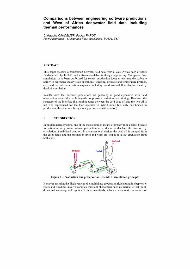
Comparisons between engineering software predictions and West of Africa deepwater field data including thermal performances Christophe CANDELIER, Fabien PAPOT Flow Assurance – Multiphase Flow specialists, TOTAL E&P ABSTRACT This paper presents a comparison between field data from a West Africa deep offshore field operated by TOTAL and software available for design engineering. Multiphase flow simulations have been performed for several production loops to evaluate the software ability to reproduce steady state operations (slugging, pressure and temperature profiles, etc.) and the full preservation sequence including shutdown and fluid displacement by dead oil circulation. Results show that software predictions are generally in good agreement with field observation especially with regards to pressure variation and timing. However the structure of the interface (i.e. mixing zone) between the cold dead oil and the live oil is not well reproduced for the loop operated in hybrid mode (i.e. only one branch in production, the other one being already preserved with dead oil). 1 INTRODUCTION In oil dominated systems, one of the most common means of preservation against hydrate formation in deep water subsea production networks is to displace the live oil by circulation of stabilized dead oil. In a conventional design, the dead oil is pumped from the cargo tanks and the production lines and risers are looped to allow circulation from both ends.

Figure 1 – Production line preservation – Dead Oil circulation principle

However ensuring the displacement of a multiphase production fluid sitting in deep water risers and flowlines involve complex transient phenomena such as thermal effect (cool-down and warm-up, cold spots effects as manifolds, subsea connectors), occurrence of

important pressure variations (depressurization, packing, unbalanced liquid head in risers) and multiphase flow effects (phase segregation, fluid displacement, liquid slugs). In design phases, it is required to model in detail the full preservation sequences to optimize the thermal specifications of the equipment and demonstrate the capabilities of the subsea system to stay free from hydrate formation during the preservation planning considered and to design relevant circulation pumps, etc. Flow Assurance engineers then use commercial multiphase flow software for the design of field development facilities. As a consequence, optimized design recommendations heavily rely on the accuracy of these multiphase flow simulators and usually require carrying out extensive sensitivity studies in order to define the expected operating envelope of the production network and to ensure its compliance with operating constraints and equipment capabilities. With increasing demand on Flow Assurance tools, developments works are performed continuously by code suppliers to improve the simulation accuracy and operators have to undertake systematic internal validation tests before qualifying released versions. Nevertheless, despite the fact that experimental databases are widely used for the assessment of the accuracy of the different mechanistic models, the final proof remains the results of comparisons between multiphase flow assurance software and actual field production data. Note that the use and access to field temperature data for the validation of thermal models is relatively limited compared to the hydrodynamic models for which development is supported using important experimental database and field production data. 2 EXPERIMENTAL DATA – A FIRST NECESSITY FOR MULTIPHASE

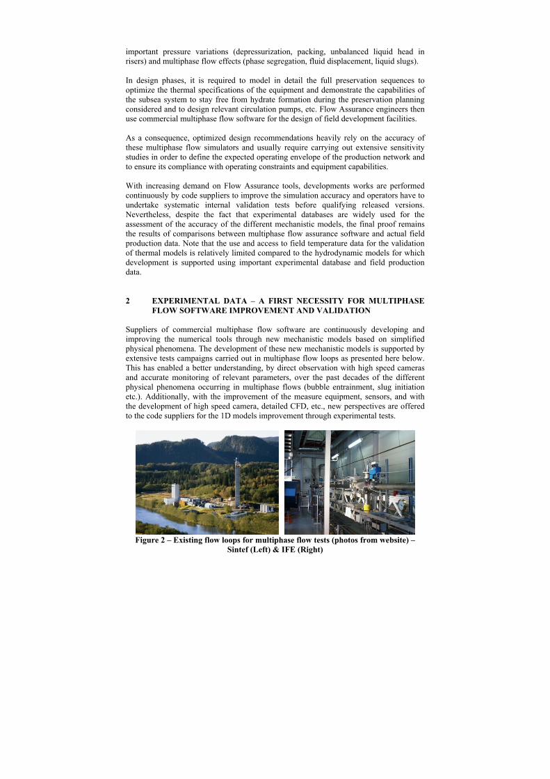
FLOW SOFTWARE IMPROVEMENT AND VALIDATION Suppliers of commercial multiphase flow software are continuously developing and improving the numerical tools through new mechanistic models based on simplified physical phenomena. The development of these new mechanistic models is supported by extensive tests campaigns carried out in multiphase flow loops as presented here below. This has enabled a better understanding, by direct observation with high speed cameras and accurate monitoring of relevant parameters, over the past decades of the different physical phenomena occurring in multiphase flows (bubble entrainment, slug initiation etc.). Additionally, with the improvement of the measure equipment, sensors, and with the development of high speed camera, detailed CFD, etc., new perspectives are offered to the code suppliers for the 1D models improvement through experimental tests.

Figure 2 – Existing flow loops for multiphase flow tests (photos from website) –

Sintef (Left) & IFE (Right)

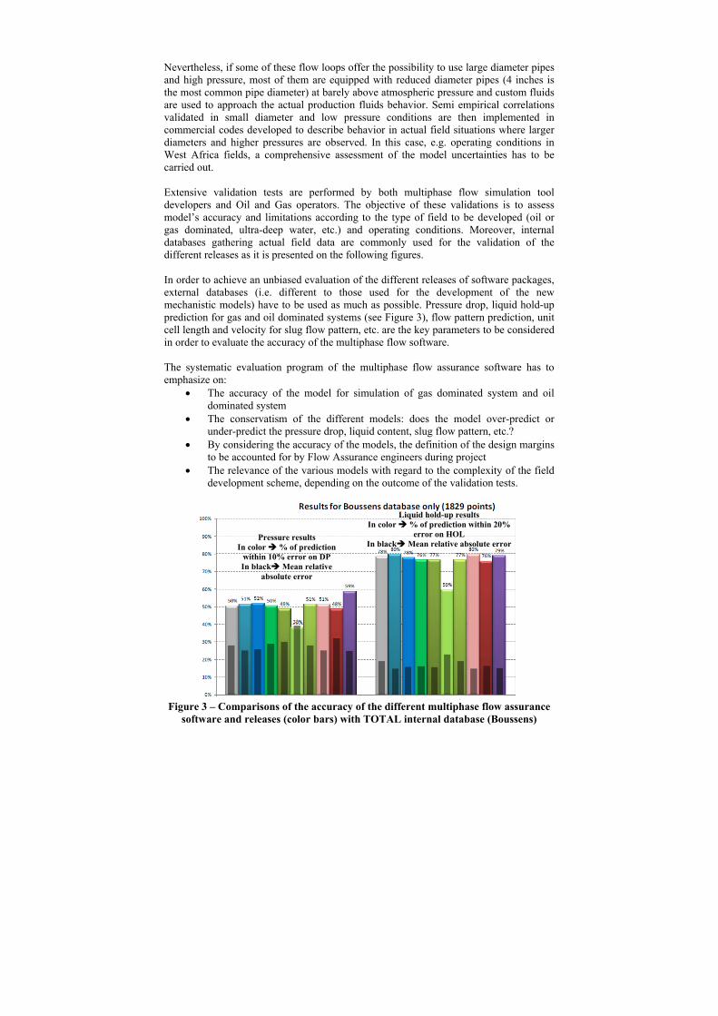
Nevertheless, if some of these flow loops offer the possibility to use large diameter pipes and high pressure, most of them are equipped with reduced diameter pipes (4 inches is the most common pipe diameter) at barely above atmospheric pressure and custom fluids are used to approach the actual production fluids behavior. Semi empirical correlations validated in small diameter and low pressure conditions are then implemented in commercial codes developed to describe behavior in actual field situations where larger diameters and higher pressures are observed. In this case, e.g. operating conditions in West Africa fields, a comprehensive assessment of the model uncertainties has to be carried out. Extensive validation tests are performed by both multiphase flow simulation tool developers and Oil and Gas operators. The objective of these validations is to assess model’s accuracy and limitations according to the type of field to be developed (oil or gas dominated, ultra-deep water, etc.) and operating conditions. Moreover, internal databases gathering actual field data are commonly used for the validation of the different releases as it is presented on the following figures. In order to achieve an unbiased evaluation of the different releases of software packages, external databases (i.e. different to those used for the development of the new mechanistic models) have to be used as much as possible. Pressure drop, liquid hold-up prediction for gas and oil dominated systems (see Figure 3), flow pattern prediction, unit cell length and velocity for slug flow pattern, etc. are the key parameters to be considered in order to evaluate the accuracy of the multiphase flow software. The systematic evaluation program of the multiphase flow assurance software has to emphasize on:

The accuracy of the model for simulation of gas dominated system and oil dominated system

The conservatism of the different models: does the model over-predict or under-predict the pressure drop, liquid content, slug flow pattern, etc.?

By considering the accuracy of the models, the definition of the design margins to be accounted for by Flow Assurance engineers during project

The relevance of the various models with regard to the complexity of the field development scheme, depending on the outcome of the validation tests.

Figure 3 – Comparisons of the accuracy of the different multiphase flow assurance

software and releases (color bars) with TOTAL internal database (Boussens)

Pressure results In color % of prediction

within 10% error on DP In black Mean relative

absolute error

Liquid hold-up results In color % of prediction within 20%

error on HOL In black Mean relative absolute error

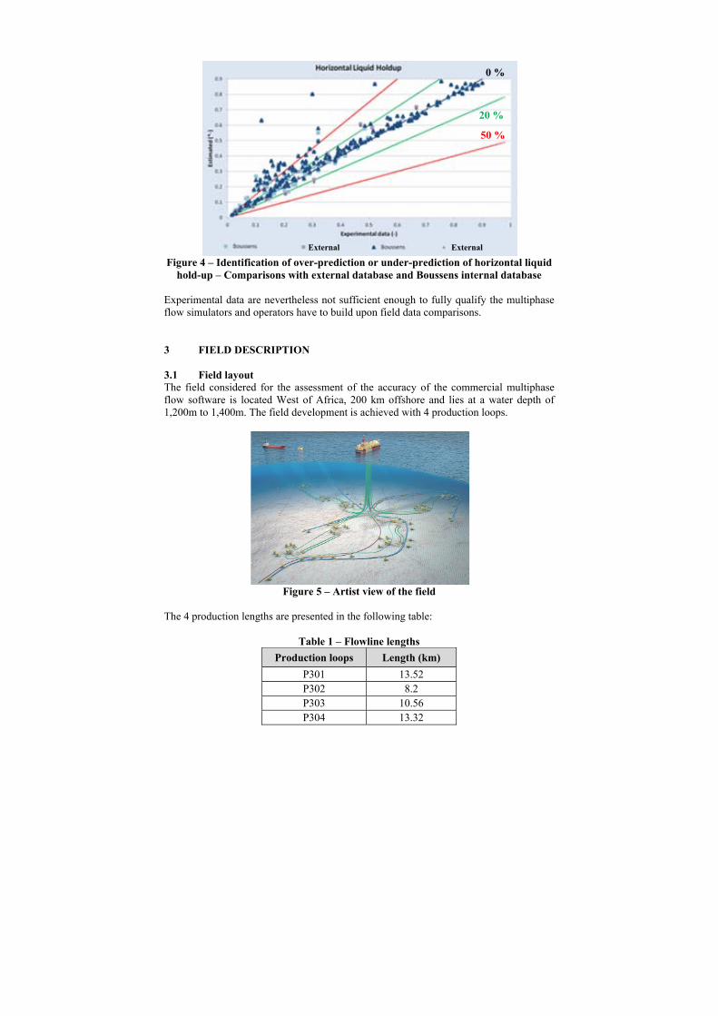
Figure 4 – Identification of over-prediction or under-prediction of horizontal liquid

hold-up – Comparisons with external database and Boussens internal database Experimental data are nevertheless not sufficient enough to fully qualify the multiphase flow simulators and operators have to build upon field data comparisons. 3 FIELD DESCRIPTION 3.1 Field layout The field considered for the assessment of the accuracy of the commercial multiphase flow software is located West of Africa, 200 km offshore and lies at a water depth of 1,200m to 1,400m. The field development is achieved with 4 production loops.

Figure 5 – Artist view of the field

The 4 production lengths are presented in the following table:

Table 1 – Flowline lengths

Production loops Length (km)

P301 13.52 P302 8.2 P303 10.56 P304 13.32

External External

50 %

20 %

0 %

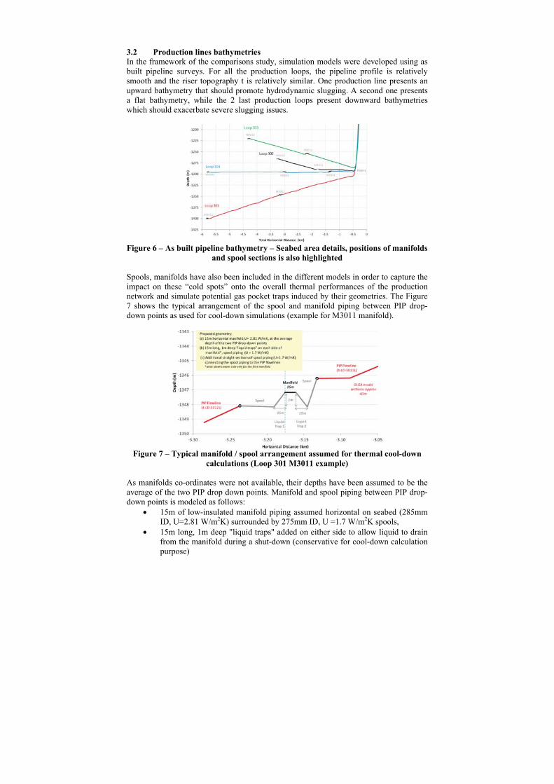
3.2 Production lines bathymetries In the framework of the comparisons study, simulation models were developed using as built pipeline surveys. For all the production loops, the pipeline profile is relatively smooth and the riser topography t is relatively similar. One production line presents an upward bathymetry that should promote hydrodynamic slugging. A second one presents a flat bathymetry, while the 2 last production loops present downward bathymetries which should exacerbate severe slugging issues.

Figure 6 – As built pipeline bathymetry – Seabed area details, positions of manifolds

and spool sections is also highlighted Spools, manifolds have also been included in the different models in order to capture the impact on these “cold spots” onto the overall thermal performances of the production network and simulate potential gas pocket traps induced by their geometries. The Figure 7 shows the typical arrangement of the spool and manifold piping between PIP drop-down points as used for cool-down simulations (example for M3011 manifold).

Figure 7 – Typical manifold / spool arrangement assumed for thermal cool-down

calculations (Loop 301 M3011 example) As manifolds co-ordinates were not available, their depths have been assumed to be the average of the two PIP drop down points. Manifold and spool piping between PIP drop-down points is modeled as follows:

15m of low-insulated manifold piping assumed horizontal on seabed (285mm ID, U=2.81 W/m2K) surrounded by 275mm ID, U =1.7 W/m2K spools,

15m long, 1m deep "liquid traps" added on either side to allow liquid to drain from the manifold during a shut-down (conservative for cool-down calculation purpose)

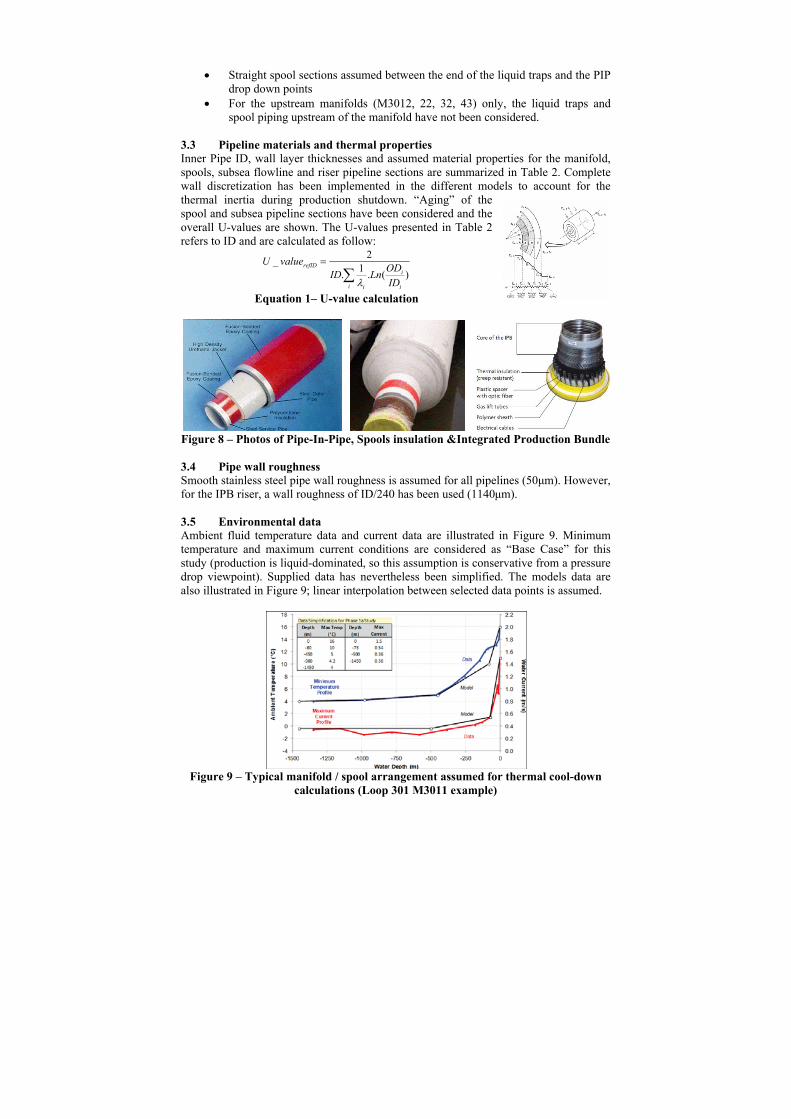
Straight spool sections assumed between the end of the liquid traps and the PIP drop down points

For the upstream manifolds (M3012, 22, 32, 43) only, the liquid traps and spool piping upstream of the manifold have not been considered.

3.3 Pipeline materials and thermal properties Inner Pipe ID, wall layer thicknesses and assumed material properties for the manifold, spools, subsea flowline and riser pipeline sections are summarized in Table 2. Complete wall discretization has been implemented in the different models to account for the thermal inertia during production shutdown. “Aging” of the spool and subsea pipeline sections have been considered and the overall U-values are shown. The U-values presented in Table 2 refers to ID and are calculated as follow:

i i

i

i

refID

IDOD

LnIDvalueU

)(.1

.

2_

     

Equation 1– U-value calculation

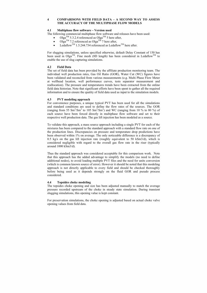
Figure 8 – Photos of Pipe-In-Pipe, Spools insulation &Integrated Production Bundle 3.4 Pipe wall roughness Smooth stainless steel pipe wall roughness is assumed for all pipelines (50μm). However, for the IPB riser, a wall roughness of ID/240 has been used (1140μm). 3.5 Environmental data Ambient fluid temperature data and current data are illustrated in Figure 9. Minimum temperature and maximum current conditions are considered as “Base Case” for this study (production is liquid-dominated, so this assumption is conservative from a pressure drop viewpoint). Supplied data has nevertheless been simplified. The models data are also illustrated in Figure 9; linear interpolation between selected data points is assumed.

Figure 9 – Typical manifold / spool arrangement assumed for thermal cool-down

calculations (Loop 301 M3011 example)

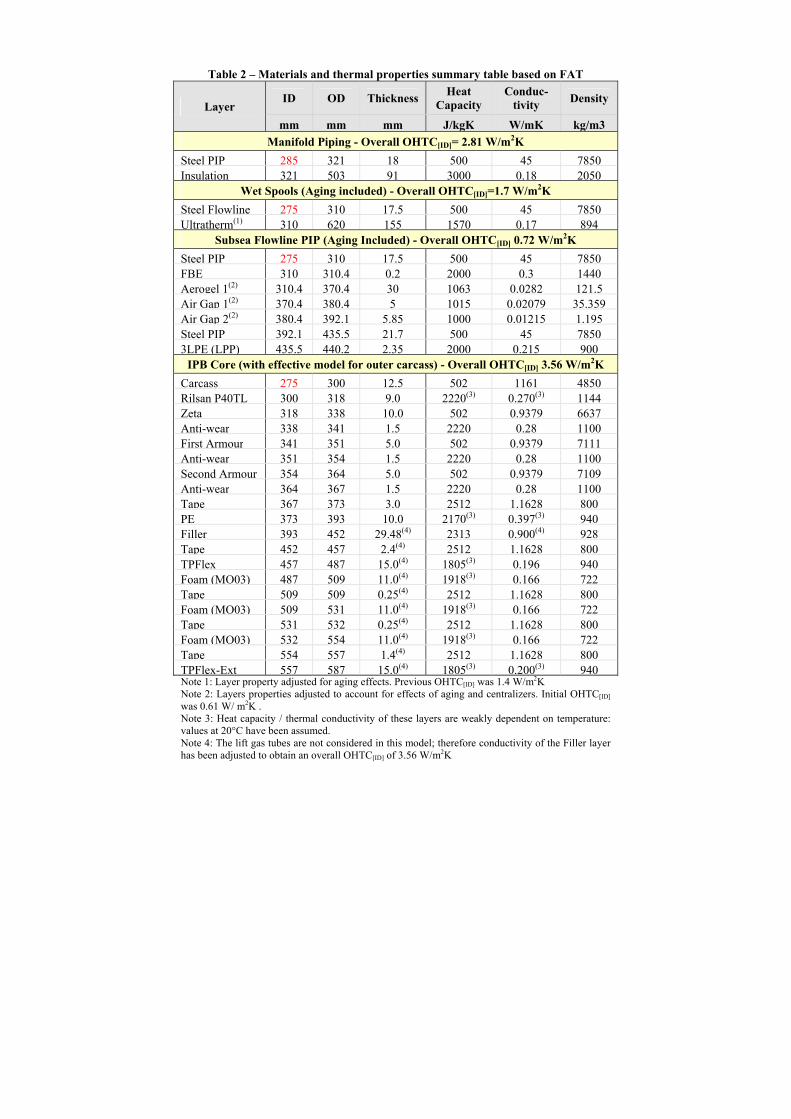
Table 2 – Materials and thermal properties summary table based on FAT

Layer ID OD Thickness

Heat Capacity

Conduc-tivity

Density

mm mm mm J/kgK W/mK kg/m3

Manifold Piping - Overall OHTC[ID]= 2.81 W/m2K

Steel PIP 285 321 18 500 45 7850 Insulation 321 503 91 3000 0.18 2050

Wet Spools (Aging included) - Overall OHTC[ID]=1.7 W/m2K

Steel Flowline 275 310 17.5 500 45 7850 Ultratherm(1) 310 620 155 1570 0.17 894

Subsea Flowline PIP (Aging Included) - Overall OHTC[ID] 0.72 W/m2K

Steel PIP 275 310 17.5 500 45 7850 FBE 310 310.4 0.2 2000 0.3 1440 Aerogel 1(2) 310.4 370.4 30 1063 0.0282 121.5 Air Gap 1(2) 370.4 380.4 5 1015 0.02079 35.359 Air Gap 2(2) 380.4 392.1 5.85 1000 0.01215 1.195 Steel PIP 392.1 435.5 21.7 500 45 7850 3LPE (LPP) 435.5 440.2 2.35 2000 0.215 900

IPB Core (with effective model for outer carcass) - Overall OHTC[ID] 3.56 W/m2K

Carcass 275 300 12.5 502 1161 4850 Rilsan P40TL 300 318 9.0 2220(3) 0.270(3) 1144 Zeta 318 338 10.0 502 0.9379 6637 Anti-wear 338 341 1.5 2220 0.28 1100 First Armour 341 351 5.0 502 0.9379 7111 Anti-wear 351 354 1.5 2220 0.28 1100 Second Armour 354 364 5.0 502 0.9379 7109 Anti-wear 364 367 1.5 2220 0.28 1100 Tape 367 373 3.0 2512 1.1628 800 PE 373 393 10.0 2170(3) 0.397(3) 940 Filler 393 452 29.48(4) 2313 0.900(4) 928 Tape 452 457 2.4(4) 2512 1.1628 800 TPFlex 457 487 15.0(4) 1805(3) 0.196 940 Foam (MO03) 487 509 11.0(4) 1918(3) 0.166 722 Tape 509 509 0.25(4) 2512 1.1628 800 Foam (MO03) 509 531 11.0(4) 1918(3) 0.166 722 Tape 531 532 0.25(4) 2512 1.1628 800 Foam (MO03) 532 554 11.0(4) 1918(3) 0.166 722 Tape 554 557 1.4(4) 2512 1.1628 800 TPFlex-Ext 557 587 15.0(4) 1805(3) 0.200(3) 940 Note 1: Layer property adjusted for aging effects. Previous OHTC[ID] was 1.4 W/m2K Note 2: Layers properties adjusted to account for effects of aging and centralizers. Initial OHTC[ID] was 0.61 W/ m2K . Note 3: Heat capacity / thermal conductivity of these layers are weakly dependent on temperature: values at 20°C have been assumed. Note 4: The lift gas tubes are not considered in this model; therefore conductivity of the Filler layer has been adjusted to obtain an overall OHTC[ID] of 3.56 W/m2K  

4 COMPARISONS WITH FIELD DATA – A SECOND WAY TO ASSESS THE ACCURACY OF THE MULTIPHASE FLOW MODELS

4.1 Multiphase flow software – Version used The following commercial multiphase flow software and releases have been used:

OlgaTM 5.3.2.4 referenced as OlgaTM 5 here after, OlgaTM 7.2 referenced as OlgaTM 7 here after, LedaflowTM 1.5.244.734 referenced as LedaflowTM here after.

For slugging simulations, unless specified otherwise, default Delay Constant of 150 has been used in OlgaTM. Fine mesh (8D length) has been considered in LedaflowTM to enable the use of slug capturing simulations. 4.2 Field Data The set of field data has been provided by the affiliate production monitoring team. The individual well production rates, Gas Oil Ratio (GOR), Water Cut (WC) figures have been validated and reconciled from various measurements (e.g. Multi Phase Flow Meter at wellhead location, well performance curves, tests separator measurement and reallocation). The pressure and temperatures trends have been extracted from the online field data historian. Note that significant efforts have been spent to gather all the required information and to ensure the quality of field data used as input to the simulation models. 4.3 PVT modeling approach For convenience purposes, a unique typical PVT has been used for all the simulations and standard conditions are used to define the flow rates of the sources. The GOR (ranging from 55 Sm3/Sm3 to 105 Sm3/Sm3) and WC (ranging from 10 % to 80 %) of each source have been forced directly in multiphase flow software and set to their respective well production data. The gas lift injection has been modeled as a source. To validate this approach, a mass source approach including a single PVT for each of the mixtures has been compared to the standard approach with a standard flow rate on one of the production lines. Discrepancies on pressure and temperature drop predictions have been observed within 1% on average. The only noticeable difference is a discrepancy of 0.5 kg/s on the gas lift injection rate (roughly equivalent to 50 kSm3/d), which is considered negligible with regard to the overall gas flow rate in the riser (typically around 1000 kSm3/d). Thus the standard approach was considered acceptable for this comparison work. Note that this approach has the added advantage to simplify the models (no need to define additional nodes), to avoid loading multiple PVT files and the need for units conversion (which is common known source of error). However it should be noted that this modeling approach is not directly applicable to every field and should be checked thoroughly before being used as it depends strongly on the fluid GOR and pseudo process considered. 4.4 Topsides choke modeling The topsides choke opening and size has been adjusted manually to match the average pressure recorded upstream of the choke in steady state simulation. During transient slugging simulations, this opening value is kept constant. For preservation simulations, the choke opening is adjusted based on actual choke valve opening values from field data.

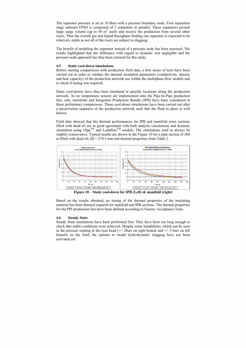
The separator pressure is set at 10 Bara with a pressure boundary node. First separation stage onboard FPSO is composed of 2 separators in parallel. These separators present large surge volume (up to 50 m3 each) and receive the production from several other risers. Thus the overall gas and liquid throughput feeding one separator is expected to be relatively stable as not all of the risers are subject to slugging. The benefit of modeling the separator instead of a pressure node has been assessed. The results highlighted that the difference with regard to dynamic was negligible and the pressure node approach has thus been retained for this study. 4.5 Static cool-down simulations Before starting comparisons with production field data, a first series of tests have been carried out in order to validate the thermal insulation parameters (conductivity, density and heat capacity) of the production network use within the multiphase flow models and to check if tuning was required. Static cool-downs have thus been simulated at specific locations along the production network. As no temperature sensors are implemented onto the Pipe-In-Pipe production line, only manifolds and Integrated Production Bundle (IPB) have been considered in these preliminary comparisons. These cool-down simulations have been carried out after a preservation sequence of the production network such that the fluid in place is well known. Field data showed that the thermal performances for IPB and manifold cross sections filled with dead oil are in good agreement with both analytic calculations and dynamic simulation using OlgaTM and LedaflowTM models. The simulations tend to always be slightly conservative. Typical results are shown in the Figure 10 for a pipe section of 200 m filled with dead oil, ID = 274.3 mm and thermal properties from Table 2.

Figure 10 – Static cool-down for IPB (Left) & manifold (right)

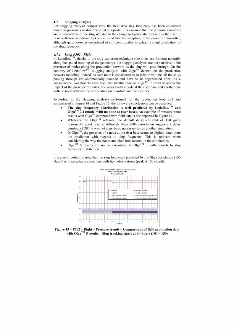
Based on the results obtained, no tuning of the thermal properties of the insulating material has been deemed required for manifold and IPB sections. The thermal properties for the PIP production line have been defined according to Factory Acceptance Tests. 4.6 Steady State Steady State simulations have been performed first. They have been run long enough to check that stable conditions were achieved. Despite some instabilities, which can be seen in the pressure reading at the riser head (+/- 2bars on right branch and +/- 5 bars on left branch) on the field, the options to model hydrodynamic slugging have not been activated yet.

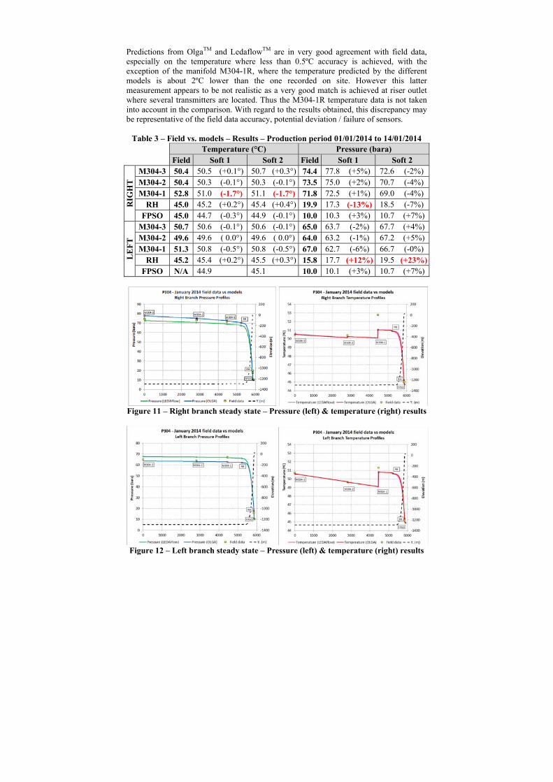
Predictions from OlgaTM and LedaflowTM are in very good agreement with field data, especially on the temperature where less than 0.5ºC accuracy is achieved, with the exception of the manifold M304-1R, where the temperature predicted by the different models is about 2ºC lower than the one recorded on site. However this latter measurement appears to be not realistic as a very good match is achieved at riser outlet where several transmitters are located. Thus the M304-1R temperature data is not taken into account in the comparison. With regard to the results obtained, this discrepancy may be representative of the field data accuracy, potential deviation / failure of sensors.

Table 3 – Field vs. models – Results – Production period 01/01/2014 to 14/01/2014 Temperature (°C) Pressure (bara) Field Soft 1 Soft 2 Field Soft 1 Soft 2

RIG

HT

M304-3 50.4 50.5 (+0.1°) 50.7 (+0.3°) 74.4 77.8 (+5%) 72.6 (-2%) M304-2 50.4 50.3 (-0.1°) 50.3 (-0.1°) 73.5 75.0 (+2%) 70.7 (-4%) M304-1 52.8 51.0 (-1.7°) 51.1 (-1.7°) 71.8 72.5 (+1%) 69.0 (-4%)

RH 45.0 45.2 (+0.2°) 45.4 (+0.4°) 19.9 17.3 (-13%) 18.5 (-7%) FPSO 45.0 44.7 (-0.3°) 44.9 (-0.1°) 10.0 10.3 (+3%) 10.7 (+7%)

LE

FT

M304-3 50.7 50.6 (-0.1°) 50.6 (-0.1°) 65.0 63.7 (-2%) 67.7 (+4%) M304-2 49.6 49.6 ( 0.0°) 49.6 ( 0.0°) 64.0 63.2 (-1%) 67.2 (+5%) M304-1 51.3 50.8 (-0.5°) 50.8 (-0.5°) 67.0 62.7 (-6%) 66.7 (-0%)

RH 45.2 45.4 (+0.2°) 45.5 (+0.3°) 15.8 17.7 (+12%) 19.5 (+23%) FPSO N/A 44.9 45.1 10.0 10.1 (+3%) 10.7 (+7%)

     Figure 11 – Right branch steady state – Pressure (left) & temperature (right) results

    Figure 12 – Left branch steady state – Pressure (left) & temperature (right) results

4.7 Slugging analysis For slugging analysis comparisons, the field data slug frequency has been calculated based on pressure variation recorded at topside. It is assumed that the pressure variations are representative of the slug size due to the change in hydrostatic pressure in the riser. It is nevertheless important to keep in mind that the sampling of the pressure transmitter, although quite loose, is considered of sufficient quality to extract a rough evaluation of the slug frequency. 4.7.1 Loop P302 - Right In LedaflowTM, thanks to the slug capturing technique (the slugs are forming naturally along the spatial meshing of the geometry), the slugging analyses are not sensitive to the presence of nodes along the production network as the slug will pass through. On the contrary of LedaflowTM, slugging analyses with OlgaTM depend on the production network modeling. Indeed, as each node is considered as an infinite volume, all the slugs passing through are automatically damped and have to be regenerated after. As a consequence, two models have been run for this case on OlgaTM in order to assess the impact of the presence of nodes: one model with a node at the riser base and another one with no node between the last production manifold and the topsides. According to the slugging analyses performed for the production loop 302 and summarized in Figure 14 and Figure 15, the following conclusions can be observed:

The slug frequency distribution is well predicted by LedaflowTM and OlgaTM 7.2 (model with no node at riser base). An example of pressure trend results with OlgaTM compared with field data is also reported in Figure 14,

Whatever the OlgaTM releases, the default delay constant of 150 gives reasonably good results. Although Shea 2004 correlation suggests a delay constant of 297, it was not considered necessary to run another simulation.

In OlgaTM, the presence of a node at the riser base seems to slightly deteriorate the prediction with regards to slug frequency. This is relevant when considering the way the nodes are taken into account in the simulations,

OlgaTM 5 results are not as consistent as OlgaTM 7 with regards to slug frequency distribution.

It is also important to note that the slug frequency predicted by the Shea correlation (155 slug/h) is in acceptable agreement with field observations (peak at 100 slug/h).

 Figure 13 – P302 – Right – Pressure trends – Comparisons of field production data

with OlgaTM 5 results – Slug tracking starts at t=4hours (DC = 150)

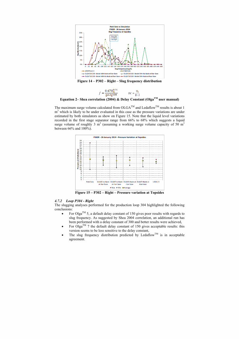
 Figure 14 – P302 – Right – Slug frequency distribution

Equation 2– Shea correlation (2004) & Delay Constant (OlgaTM user manual)

The maximum surge volume calculated from OLGATM and LedaflowTM results is about 1 m3 which is likely to be under evaluated in this case as the pressure variations are under estimated by both simulators as show on Figure 15. Note that the liquid level variations recorded in the first stage separator range from 66% to 68% which suggests a liquid surge volume of roughly 3 m3 (assuming a working surge volume capacity of 50 m3 between 66% and 100%).

Figure 15 – P302 – Right – Pressure variation at Topsides

4.7.2 Loop P304 - Right The slugging analyses performed for the production loop 304 highlighted the following conclusions:

For OlgaTM 5, a default delay constant of 150 gives poor results with regards to slug frequency. As suggested by Shea 2004 correlation, an additional run has been performed with a delay constant of 300 and better results were achieved,

For OlgaTM 7 the default delay constant of 150 gives acceptable results: this version seems to be less sensitive to the delay constant,

The slug frequency distribution predicted by LedaflowTM is in acceptable agreement.

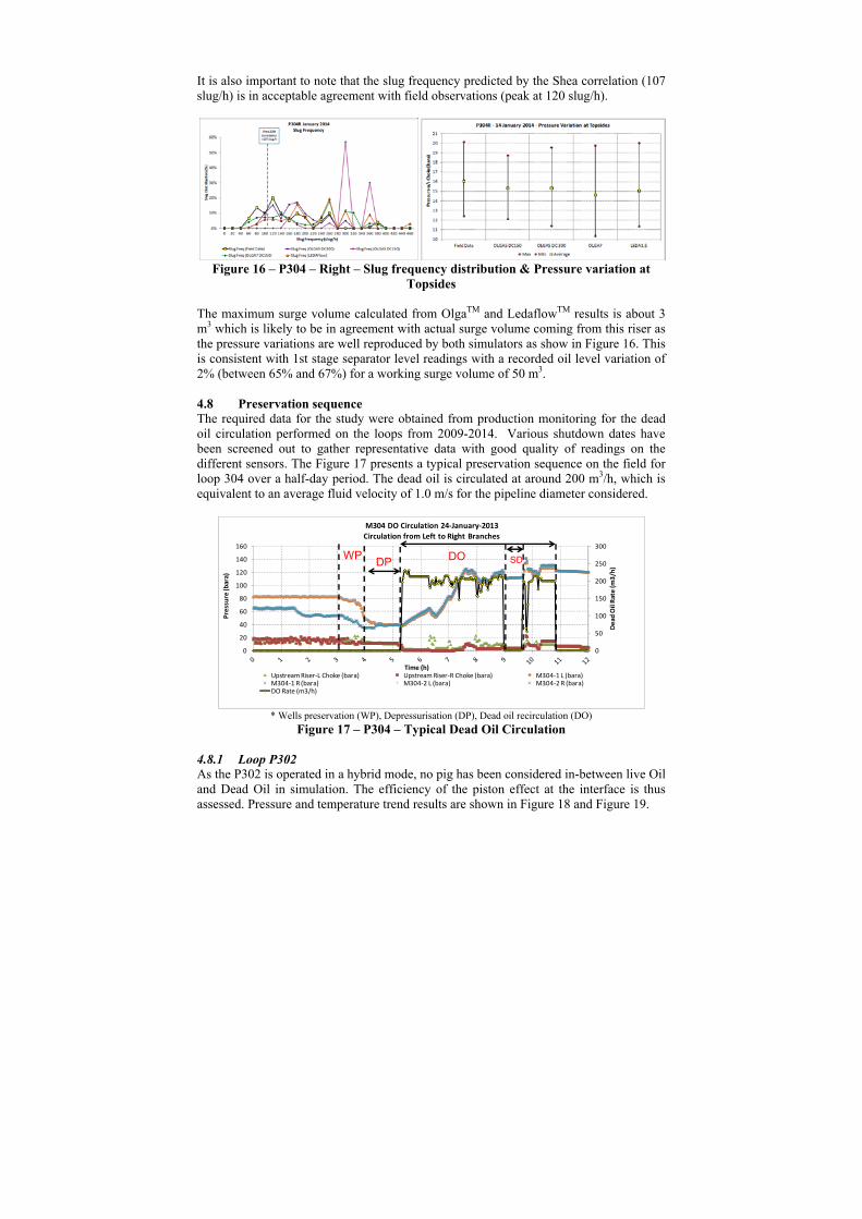
It is also important to note that the slug frequency predicted by the Shea correlation (107 slug/h) is in acceptable agreement with field observations (peak at 120 slug/h).

Figure 16 – P304 – Right – Slug frequency distribution & Pressure variation at

Topsides The maximum surge volume calculated from OlgaTM and LedaflowTM results is about 3 m3 which is likely to be in agreement with actual surge volume coming from this riser as the pressure variations are well reproduced by both simulators as show in Figure 16. This is consistent with 1st stage separator level readings with a recorded oil level variation of 2% (between 65% and 67%) for a working surge volume of 50 m3. 4.8 Preservation sequence The required data for the study were obtained from production monitoring for the dead oil circulation performed on the loops from 2009-2014. Various shutdown dates have been screened out to gather representative data with good quality of readings on the different sensors. The Figure 17 presents a typical preservation sequence on the field for loop 304 over a half-day period. The dead oil is circulated at around 200 m3/h, which is equivalent to an average fluid velocity of 1.0 m/s for the pipeline diameter considered.

* Wells preservation (WP), Depressurisation (DP), Dead oil recirculation (DO)

Figure 17 – P304 – Typical Dead Oil Circulation 4.8.1 Loop P302 As the P302 is operated in a hybrid mode, no pig has been considered in-between live Oil and Dead Oil in simulation. The efficiency of the piston effect at the interface is thus assessed. Pressure and temperature trend results are shown in Figure 18 and Figure 19.

0

50

100

150

200

250

300

0

20

40

60

80

100

120

140

160

Dead

 Oil Rate (m

3/h)

Pressure (bara)

Time (h)

M304 DO Circulation 24‐January‐2013

Circulation from Left to Right Branches

Upstream Riser‐L Choke (bara) Upstream Riser‐R Choke (bara) M304‐1 L (bara)M304‐1 R (bara) M304‐2 L (bara) M304‐2 R (bara)DO Rate (m3/h)

DODP SDWP

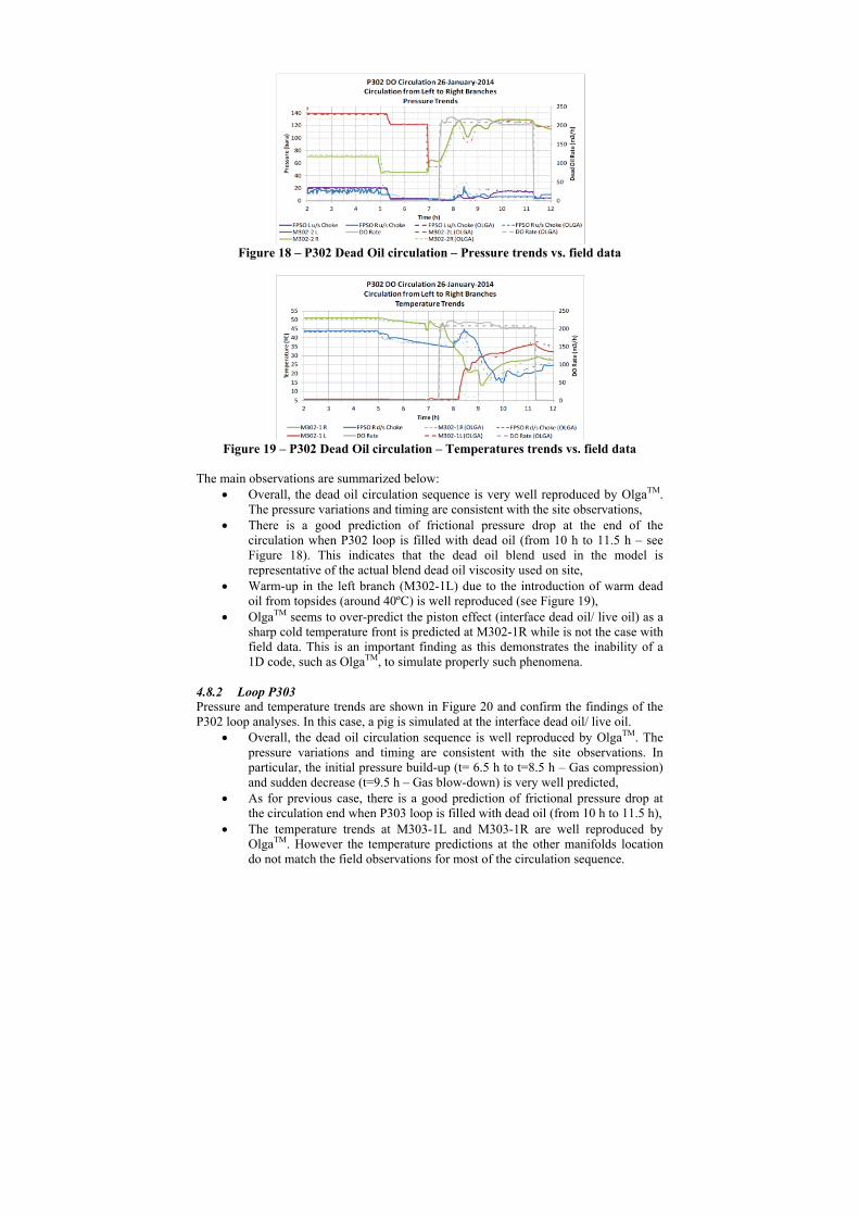
Figure 18 – P302 Dead Oil circulation – Pressure trends vs. field data

Figure 19 – P302 Dead Oil circulation – Temperatures trends vs. field data

The main observations are summarized below:

Overall, the dead oil circulation sequence is very well reproduced by OlgaTM. The pressure variations and timing are consistent with the site observations,

There is a good prediction of frictional pressure drop at the end of the circulation when P302 loop is filled with dead oil (from 10 h to 11.5 h – see Figure 18). This indicates that the dead oil blend used in the model is representative of the actual blend dead oil viscosity used on site,

Warm-up in the left branch (M302-1L) due to the introduction of warm dead oil from topsides (around 40ºC) is well reproduced (see Figure 19),

OlgaTM seems to over-predict the piston effect (interface dead oil/ live oil) as a sharp cold temperature front is predicted at M302-1R while is not the case with field data. This is an important finding as this demonstrates the inability of a 1D code, such as OlgaTM, to simulate properly such phenomena.

4.8.2 Loop P303 Pressure and temperature trends are shown in Figure 20 and confirm the findings of the P302 loop analyses. In this case, a pig is simulated at the interface dead oil/ live oil.

Overall, the dead oil circulation sequence is well reproduced by OlgaTM. The pressure variations and timing are consistent with the site observations. In particular, the initial pressure build-up (t= 6.5 h to t=8.5 h – Gas compression) and sudden decrease (t=9.5 h – Gas blow-down) is very well predicted,

As for previous case, there is a good prediction of frictional pressure drop at the circulation end when P303 loop is filled with dead oil (from 10 h to 11.5 h),

The temperature trends at M303-1L and M303-1R are well reproduced by OlgaTM. However the temperature predictions at the other manifolds location do not match the field observations for most of the circulation sequence.

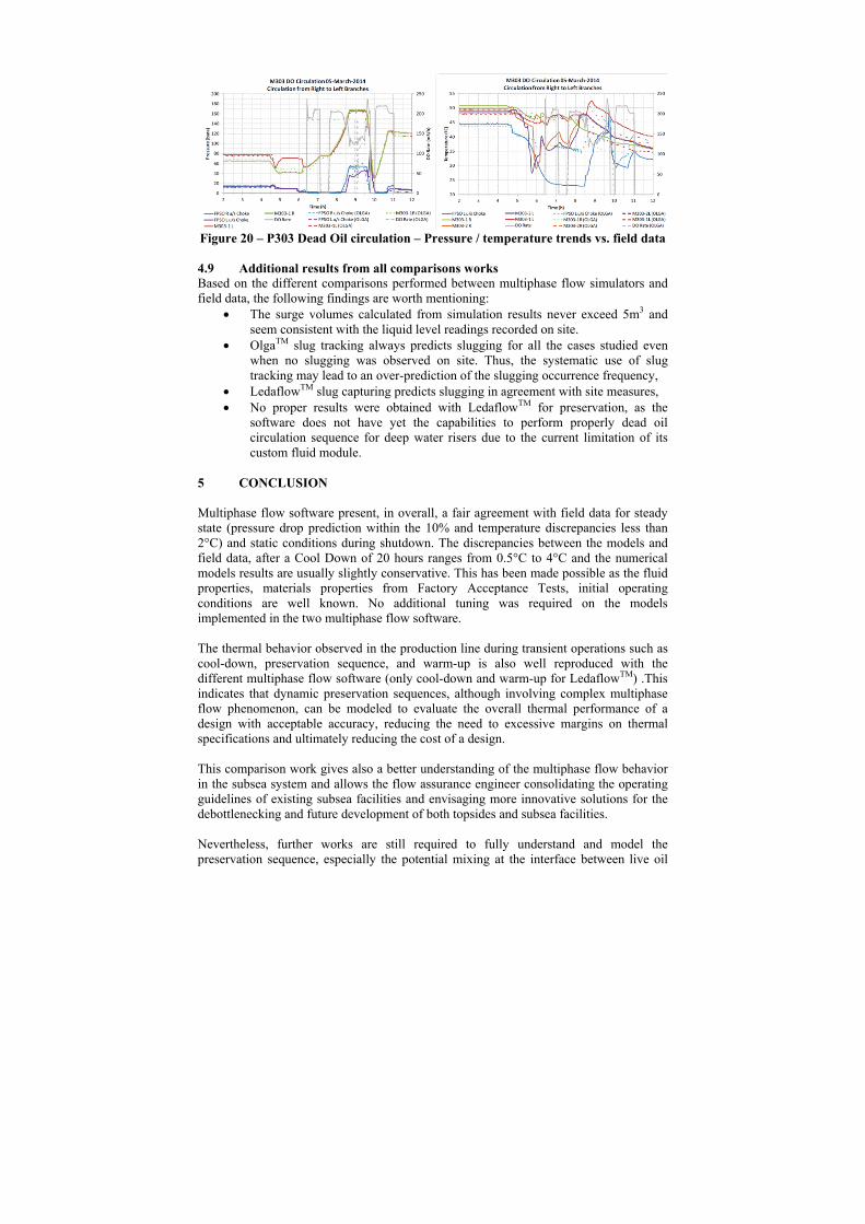
Figure 20 – P303 Dead Oil circulation – Pressure / temperature trends vs. field data 4.9 Additional results from all comparisons works Based on the different comparisons performed between multiphase flow simulators and field data, the following findings are worth mentioning:

The surge volumes calculated from simulation results never exceed 5m3 and seem consistent with the liquid level readings recorded on site.

OlgaTM slug tracking always predicts slugging for all the cases studied even when no slugging was observed on site. Thus, the systematic use of slug tracking may lead to an over-prediction of the slugging occurrence frequency,

LedaflowTM slug capturing predicts slugging in agreement with site measures, No proper results were obtained with LedaflowTM for preservation, as the

software does not have yet the capabilities to perform properly dead oil circulation sequence for deep water risers due to the current limitation of its custom fluid module.

5 CONCLUSION Multiphase flow software present, in overall, a fair agreement with field data for steady state (pressure drop prediction within the 10% and temperature discrepancies less than 2°C) and static conditions during shutdown. The discrepancies between the models and field data, after a Cool Down of 20 hours ranges from 0.5°C to 4°C and the numerical models results are usually slightly conservative. This has been made possible as the fluid properties, materials properties from Factory Acceptance Tests, initial operating conditions are well known. No additional tuning was required on the models implemented in the two multiphase flow software. The thermal behavior observed in the production line during transient operations such as cool-down, preservation sequence, and warm-up is also well reproduced with the different multiphase flow software (only cool-down and warm-up for LedaflowTM) .This indicates that dynamic preservation sequences, although involving complex multiphase flow phenomenon, can be modeled to evaluate the overall thermal performance of a design with acceptable accuracy, reducing the need to excessive margins on thermal specifications and ultimately reducing the cost of a design. This comparison work gives also a better understanding of the multiphase flow behavior in the subsea system and allows the flow assurance engineer consolidating the operating guidelines of existing subsea facilities and envisaging more innovative solutions for the debottlenecking and future development of both topsides and subsea facilities. Nevertheless, further works are still required to fully understand and model the preservation sequence, especially the potential mixing at the interface between live oil

and dead oil. These studies should rely on finer mesh discretization in 1D model to better capture the front if any at the interface. With the boom of full 3D models in the Oil & Gas industry, and the spread of the access to high CPU resources, CFD modeling might be also considered. Whatever the solution retained, long CPU time should be expected. As a matter of fact, TOTAL E&P has fostered an acknowledged expertise and technical advances in Flow Assurance leading the Group to conduct bold developments especially in deepwater fields. ABBREVIATIONS CFD Computational Fluid Dynamic CPU Central Processing Unit DC Delay Constant DO Dead Oil DP Pressure Drop FPSO Floating Production Storage Offloading GOR Gas Oil Ratio HOL Liquid Hold-up ID Internal Diameter IPB Integrated Production Bundle OHTC Overall Heat Transfer Coefficient OP Outside Diameter PIP Pipe In Pipe RH Riser Head WC Water Cut WP Wells preservation λ Thermal conductivity of insulating material ACKNOWLEDGEMENTS The authors gratefully acknowledge the support and encouragement they receive from TOTAL E&P while preparing this manuscript. REFERENCES [1] Fabre J. a Liné A., 1992, Modeling of two phases slug flow, Annual review of fluid mechanics, 24, 21-46 [2] Valluri P., Spelt P.D.M., Lawrence C.J., Hewitt G.F., 2008, Numerical simulation of the onset of slug initiation in laminar horizontal channel flow, International Journal of multiphase flow 34 206 – 225 [3] E. Al-Safran, 2009, Investigation and prediction of slug frequency in Gas / Liquid horizontal pipe flow, Journal of petroleum science and engineering 69 (2009) 143 – 155 [4] G.J. Zabaras, 2000, Prediction of slug frequency for Gas / Liquid flows, SPE journal 5 (3), September 2000 [5] T. Danielson, K. Bansal, B. Djoric, D. Larrey, S.T. Johansen, A. de Leedbeeck, J. Kjolaas, 2012, Simulation of slug flow in Oil and Gas pipelines using a new transient simulator, OTC 23353 [6] R. Belt, B. Djoric, S. Kalali, E. Duret, D. Larrey, 2011, Comparison of commercial multiphase flow simulators with experimental and field databases, BHRG conference.

Comparisons between engineering software predictions and West of Africa deepwater field data including thermal performances

Christophe CANDELIER & Fabien PAPOT

Flow Assurance specialists – TOTAL E&P

Introduction • World’s largest and easiest to exploit deepwater

field already under production

• Hydrates among the worst fluid chemistry issues

– Not critical in production - Mainly expected during transient operations (shutdown and well restart)

– Hydrates prevention with specific operating procedures and with specific subsea architecture (production loop, etc.)

• Preservation sequence principle

– Live oil displacement with Dead oil

– Complex transient phenomena observed

• Thermal effect (cool down, etc.)

• Important pressure variations (depressurization, etc.)

• Multiphase flow effects (segregation, surge, etc.)

Flow Assurance in design phases • Full preservation sequences

– Modeled in detail

– Support the definition of the thermal insulation specifications of the different subsea equipment (Wellhead, manifold, production lines, spools, etc.)

– Design of auxiliaries equipment (circulation pumps, emergency generator, etc.)

– TOTAL’s design principle : Stay free from hydrate formation

Design recommendations heavily rely on the accuracy of the multiphase flow software used during design phases

Extensive sensitivity studies performed to: • Define operating envelope of the network • Ensure compliance with operating constraints

Extensive internal validation tests performed to assess the accuracy of software • Comparisons to experimental database • Comparisons to field production data

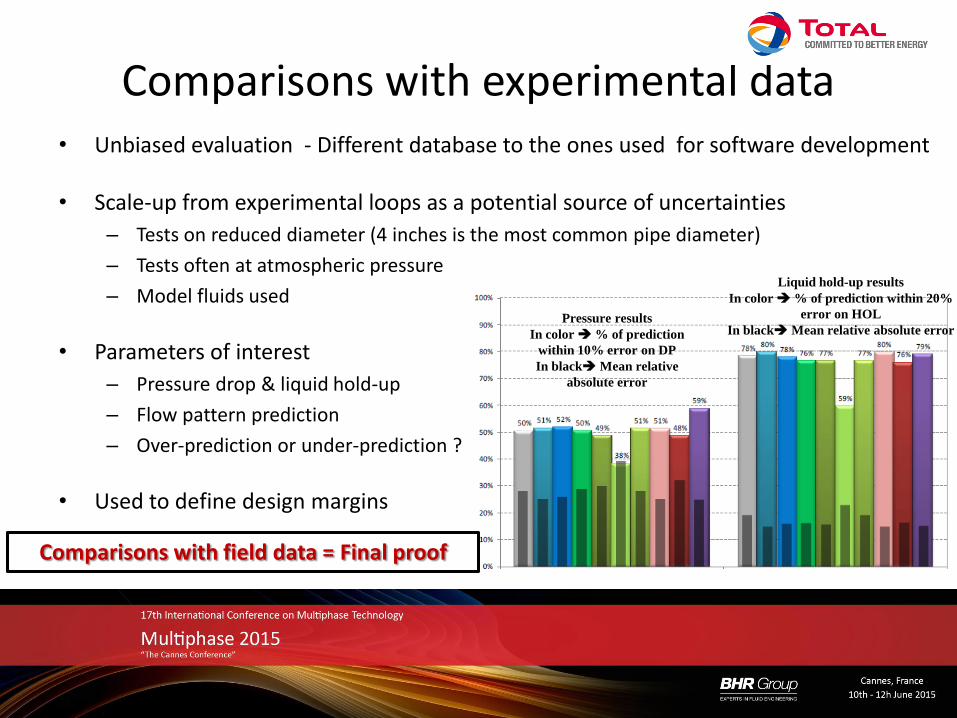
Comparisons with experimental data

Pressure results

In color % of prediction

within 10% error on DP

In black Mean relative

absolute error

Liquid hold-up results

In color % of prediction within 20%

error on HOL

In black Mean relative absolute error

• Unbiased evaluation - Different database to the ones used for software development

• Scale-up from experimental loops as a potential source of uncertainties

– Tests on reduced diameter (4 inches is the most common pipe diameter)

– Tests often at atmospheric pressure

– Model fluids used

• Parameters of interest

– Pressure drop & liquid hold-up

– Flow pattern prediction

– Over-prediction or under-prediction ?

• Used to define design margins

Comparisons with field data = Final proof

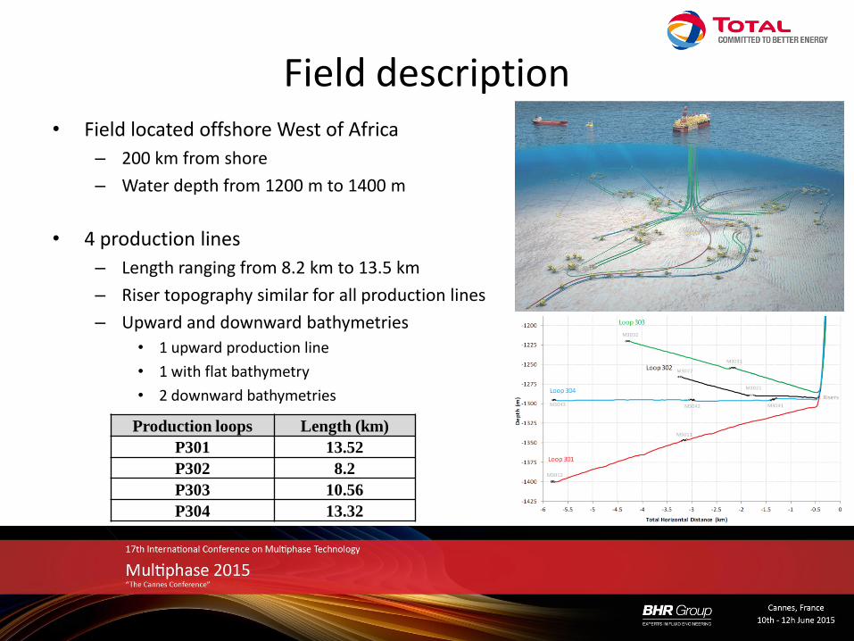
Field description • Field located offshore West of Africa

– 200 km from shore

– Water depth from 1200 m to 1400 m

• 4 production lines

– Length ranging from 8.2 km to 13.5 km

– Riser topography similar for all production lines

– Upward and downward bathymetries

• 1 upward production line

• 1 with flat bathymetry

• 2 downward bathymetries

Production loops Length (km)

P301 13.52

P302 8.2

P303 10.56

P304 13.32

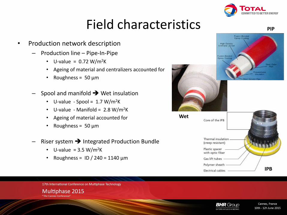
Field characteristics • Production network description

– Production line – Pipe-In-Pipe

• U-value = 0.72 W/m2K

• Ageing of material and centralizers accounted for

• Roughness = 50 µm

– Spool and manifold Wet insulation

• U-value - Spool = 1.7 W/m2K

• U-value - Manifold = 2.8 W/m2K

• Ageing of material accounted for

• Roughness = 50 µm

– Riser system Integrated Production Bundle

• U-value = 3.5 W/m2K

• Roughness = ID / 240 = 1140 µm

IPB

Wet

PIP

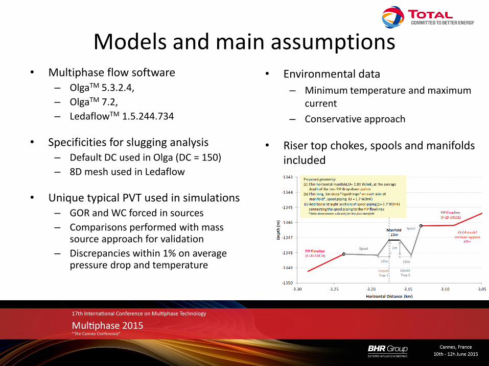
Models and main assumptions • Multiphase flow software

– OlgaTM 5.3.2.4,

– OlgaTM 7.2,

– LedaflowTM 1.5.244.734

• Specificities for slugging analysis – Default DC used in Olga (DC = 150)

– 8D mesh used in Ledaflow

• Unique typical PVT used in simulations – GOR and WC forced in sources

– Comparisons performed with mass source approach for validation

– Discrepancies within 1% on average pressure drop and temperature

• Environmental data

– Minimum temperature and maximum current

– Conservative approach

• Riser top chokes, spools and manifolds included

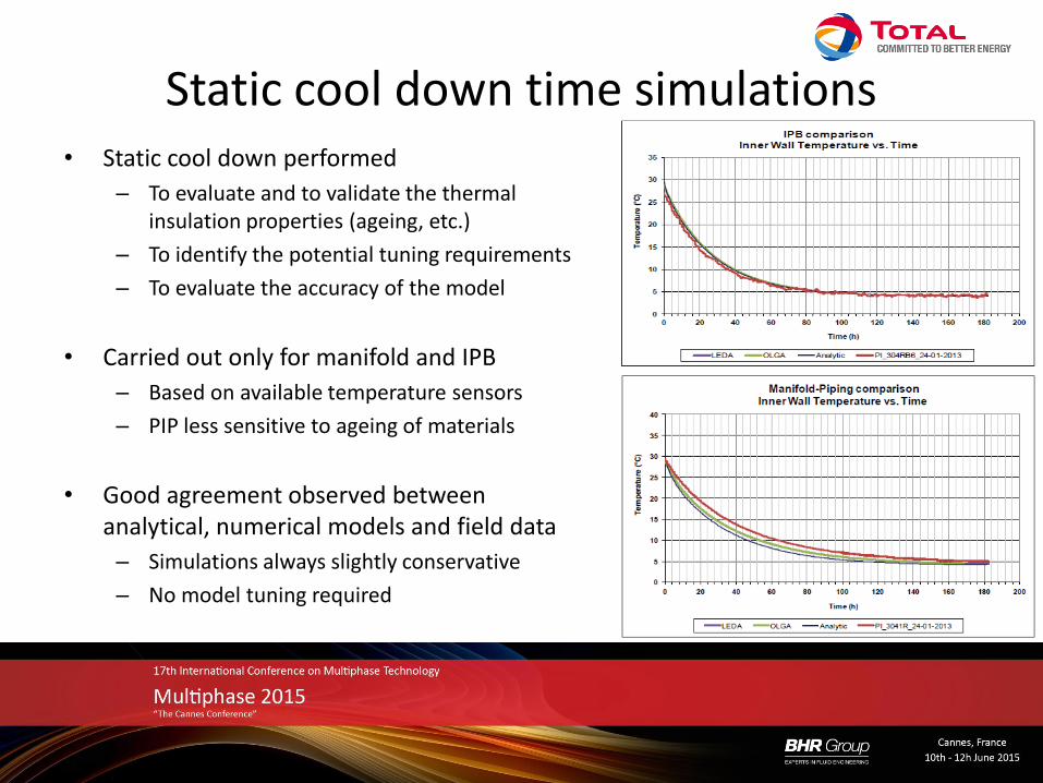
Static cool down time simulations • Static cool down performed

– To evaluate and to validate the thermal insulation properties (ageing, etc.)

– To identify the potential tuning requirements

– To evaluate the accuracy of the model

• Carried out only for manifold and IPB

– Based on available temperature sensors

– PIP less sensitive to ageing of materials

• Good agreement observed between analytical, numerical models and field data

– Simulations always slightly conservative

– No model tuning required

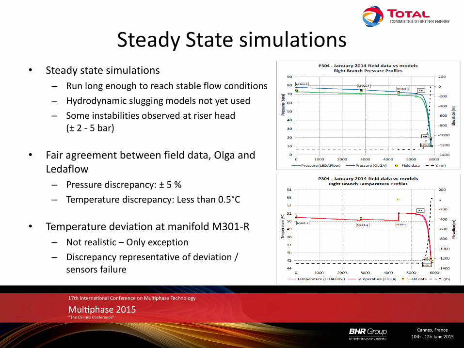
Steady State simulations • Steady state simulations

– Run long enough to reach stable flow conditions

– Hydrodynamic slugging models not yet used

– Some instabilities observed at riser head (± 2 - 5 bar)

• Fair agreement between field data, Olga and Ledaflow

– Pressure discrepancy: ± 5 %

– Temperature discrepancy: Less than 0.5°C

• Temperature deviation at manifold M301-R

– Not realistic – Only exception

– Discrepancy representative of deviation / sensors failure

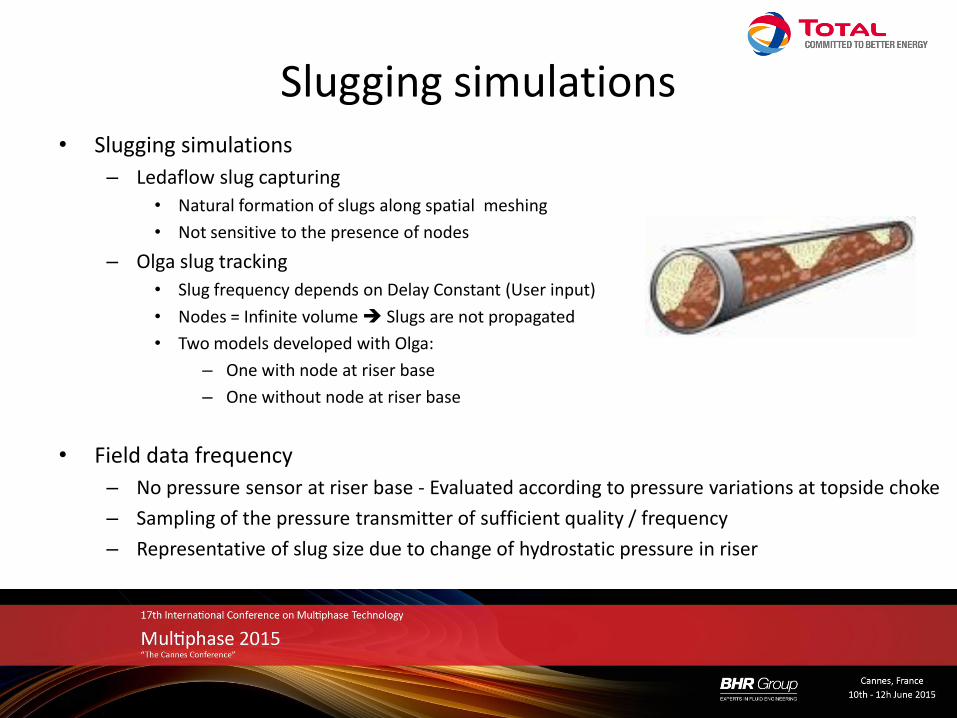
Slugging simulations • Slugging simulations

– Ledaflow slug capturing

• Natural formation of slugs along spatial meshing

• Not sensitive to the presence of nodes

– Olga slug tracking

• Slug frequency depends on Delay Constant (User input)

• Nodes = Infinite volume Slugs are not propagated

• Two models developed with Olga:

– One with node at riser base

– One without node at riser base

• Field data frequency

– No pressure sensor at riser base - Evaluated according to pressure variations at topside choke

– Sampling of the pressure transmitter of sufficient quality / frequency

– Representative of slug size due to change of hydrostatic pressure in riser

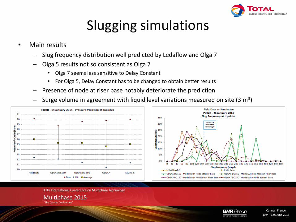
Slugging simulations • Main results

– Slug frequency distribution well predicted by Ledaflow and Olga 7

– Olga 5 results not so consistent as Olga 7

• Olga 7 seems less sensitive to Delay Constant

• For Olga 5, Delay Constant has to be changed to obtain better results

– Presence of node at riser base notably deteriorate the prediction

– Surge volume in agreement with liquid level variations measured on site (3 m3)

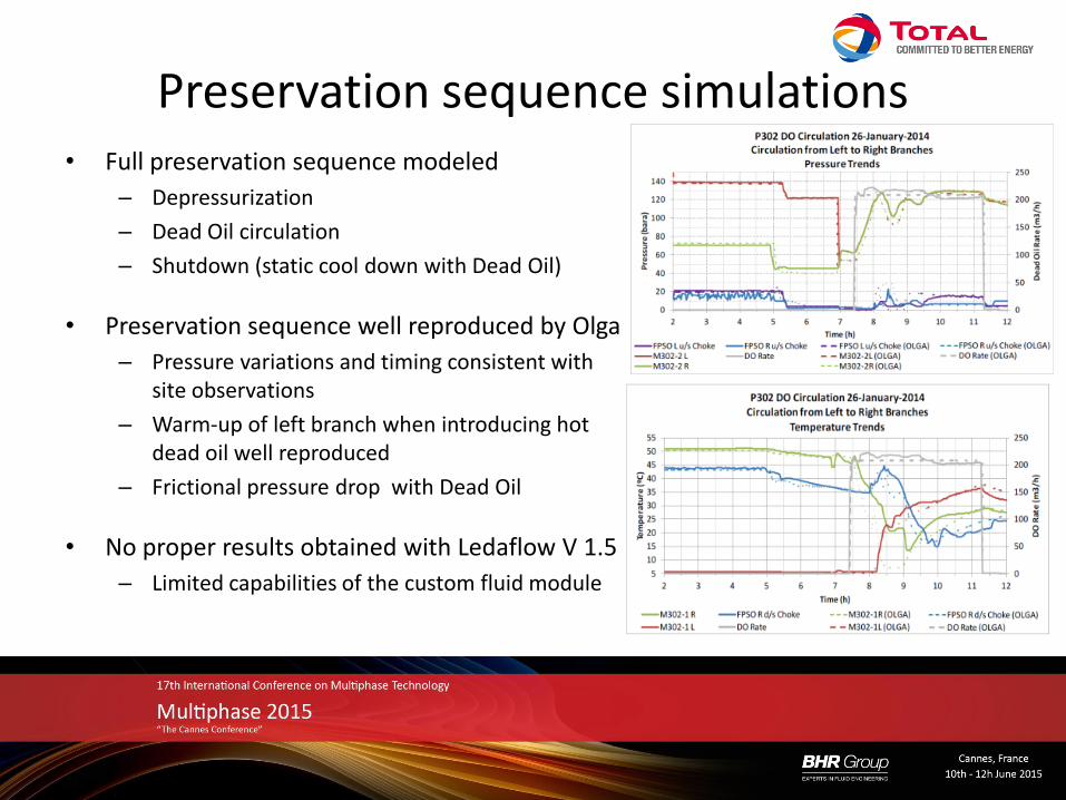
Preservation sequence simulations • Full preservation sequence modeled

– Depressurization

– Dead Oil circulation

– Shutdown (static cool down with Dead Oil)

• Preservation sequence well reproduced by Olga

– Pressure variations and timing consistent with site observations

– Warm-up of left branch when introducing hot dead oil well reproduced

– Frictional pressure drop with Dead Oil

• No proper results obtained with Ledaflow V 1.5

– Limited capabilities of the custom fluid module

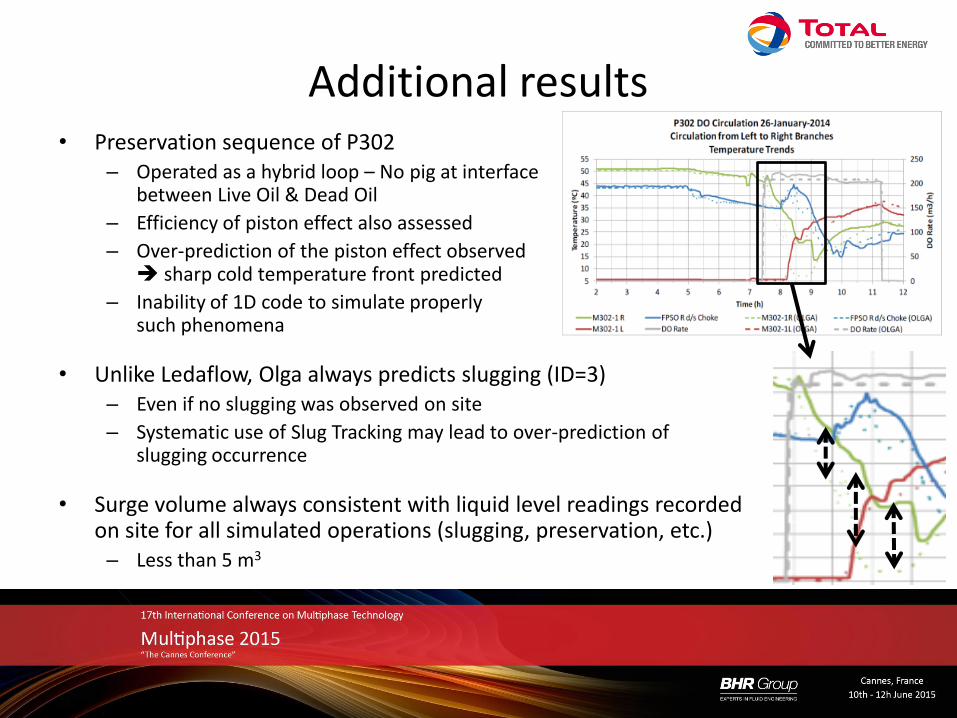
Additional results • Preservation sequence of P302

– Operated as a hybrid loop – No pig at interface between Live Oil & Dead Oil

– Efficiency of piston effect also assessed

– Over-prediction of the piston effect observed sharp cold temperature front predicted

– Inability of 1D code to simulate properly such phenomena

• Unlike Ledaflow, Olga always predicts slugging (ID=3) – Even if no slugging was observed on site

– Systematic use of Slug Tracking may lead to over-prediction of slugging occurrence

• Surge volume always consistent with liquid level readings recorded on site for all simulated operations (slugging, preservation, etc.) – Less than 5 m3

Conclusions • In overall, numerical simulations by both software of complex multiphase flow

phenomena present a fair agreement with field data – For steady state Pressure drop within 10% / Temperature difference less than 0.5°C

– For slugging Slug frequency in agreement with field data

– For shutdown (static cool down) Numerical model slightly conservative / Discrepancy after 20 hours ranging from 0.5°C to 4°C.

• Ledaflow slug capturing predicts slugging in agreement with site measures without specific tuning

• Confidence in results obtained when simulating dynamic preservation sequences – Confirmation of actual thermal performance of equipment

– Consolidation of operating guidelines

• Perspectives – Optimization of thermal specifications of the subsea equipment

– Can allow unlocking reserves by proposing innovative architectures and preservation procedures