Cryogenic Line Cooldown Comparison with Test Data 

Revision 0;  May 7, 2009 

Reference:  J. A. Brennan et al, “COOLDOWN OF CRYOGENIC TRANSFER LINES‐‐AN EXPERIMENTAL REPORT,” NBS (now NIST) Report 9264, November 7, 1966. 

Purpose and Overview The amount of liquid cryogen required to chill down lines, tanks, turbopumps, etc. from room temperature is often of significant importance. The physical phenomena involved can be complex, including film boiling and transition boiling, and two‐phase pressure drops. Pressure surges can also be experienced when liquid, insulated by a layer of vapor film in the “inverted annular” regime, strikes a bend or obstruction downstream and boils explosively. However, the focus of this study is not on such hydrodynamic events, but rather on the longer time scale thermodynamic events: the time and liquid required to quench a line. 

Simulations were made using SINDA/FLUINT V5.2, based in both the Sinaps© nongeometric (sketchpad) GUI and the Thermal Desktop© with FloCAD© geometric (CAD‐based) GUI. Since all models are available for inspection and for use as a starting point or template, only brief descriptions are included in this document as general guidance. A basic understanding of SINDA/FLUINT modeling is assumed. 

The primary purpose of this study was to ascertain the suitability of various SINDA/FLUINT assumptions and methods when applied to such cases, including a quantitative estimate of the uncertainties involved such that appropriate conservatism can be applied to the design. Typically, this conservatism takes the form of allocating additional cryogenic liquid as needed to assure the chilling and filling of the line despite the uncertainties involved. 

In particular, SINDA/FLUINT provides a set of default correlations for heat transfer and pressure drop that, being general‐purpose and fluid‐independent, may or may not be applicable to each new modeling need. While these correlations can be easily modified or replaced by the analyst, such extra effort is often neglected. One of the subpurposes of this study was to attempt to identify which if any defaults may be inappropriate for cryogenic quenching problems. Another subpurpose was to demonstrate the use of variational methods that are readily available within SINDA/FLUINT for exploring such uncertainties. 

Summary of the NBS Report 9264 A PDF scan of the original report is available. Therefore, this section provides only a brief summary. 

A series of cooldown tests was conducted whose focus was the investigation of pressure surges within a room temperature line when liquid cryogen is injected into it from one end. The line was a copper vacuum‐jacketed pipe: 1.59cm ID and 1.90cm OD, 61m long. The source was a 300 liter tank that was 

filled with either liquid hydrogen or liquid nitrogen. The opposite end of the line was open to the atmosphere (approx. 0.82 atmosphere in Boulder, Colorado). At time zero a valve was opened, allowing liquid to flow into the line. Pressure and temperature histories were recorded at 4 stations along the line (6.1m, 24.4m, 43m, and 60.4m from the supply tank). 

The figure below was extracted from Figure 1 of the NBS report.  

 

The fluid within the supply dewar was either (1) pressurized and allowed to come to approximate thermal equilibrium at that pressure (“saturated”), or was (2) quickly pressurized from saturation at atmospheric pressure (“subcooled”). 

Some of the ambiguities or uncertainties in the report, and their relative importance, are discussed below: 

1. The initial temperature of the liquid is unknown, despite the declaration of “saturated” or “subcooled.” However, a reasonable value can be guessed from the test data, and the results are not very sensitive to this uncertainty. 

2. The nature of the pressurizing gas, though presumed to be helium, is unknown, as is the hold time. Dissolution/evolution of the gas is therefore neglected, and the consistent trend between saturated and subcooled runs (at least for hydrogen) is taken as an indication that this effect is indeed negligible. (The presumption here is that the subcooled runs should be nearly free of dissolved gas since the hold times must have been very short.) 

3. The type of valve used for each test is unknown. However, since the focus of this study is on longer time‐scale events, and since the results were insensitive to the small magnitude of pressure losses associated with each valve, this unknown is not important. A ball valve (very low resistance) was assumed for most analyses reported. Valve opening times were assumed instantaneous. 

4. The nature of the vacuum‐jacketed shield is unknown, but the results are largely insensitive to variations in the model of this insulation. 

5. The material specification for the copper line is missing. While the thermal conductivity of various alloys is highly variable, that particular property does not have much effect on results. More important is the specific heat, but fortunately variations between alloys are relatively small: on the order of 5% or less. OFHC copper was used as a baseline (even though it would have likely been unavailable in drawn tubing) and uncertainties in the specific heat were explored analytically. 

6. The accuracy of the supply pressure and the line temperature measurements is unknown. There are clear indications of problems in the thermistry based on inconsistent results. (This is noted in the NBS report.1) 

7. The amount of initial fill of liquid in the supply tank is uncertain, and pressures can drop during the run due to depletion (expansion of the ullage). The volume of the line is 12 liters compared to 300 liters in the supply tank, but it can take perhaps 30‐50 liters of liquid hydrogen to accomplish the cooldown event. This effect (i.e., the added uncertainty in the supply pressure) is more important for hydrogen runs than for nitrogen runs, since the amount of liquid nitrogen required is much less (about 15‐20 liters). 

                                                            1  The crossing of lines at cold temperatures was noted in the NBS report as an indication of measurement error. For example, station 3 often stayed warmer than station 4, which was downstream of it. Interestingly, some of this discrepancy actually has a physical explanation that the NBS authors did not appear to consider. In saturated runs, or in downstream sections, the liquid continues to flash as the pressure drops. This means that while both stations 3 and 4 might contain mostly liquid, they are at different pressures, and so different saturation conditions. Therefore, station 4 should be colder since it is nearer the exit (and so at a lower pressure than is station 3). 

8. The relative amount of para versus ortho hydrogen is unknown. This turns out to be a cause of significant uncertainty in the results for hydrogen cases, as will be explained in detail below. 

9. The ID and roughness of the tube are uncertain. The classification of the tube is not known, and the dimensions do not correspond to currently available off‐the‐shelf options. While the roughness uncertainty is not significant, one percent uncertainty (i.e., on the order the manufacturing tolerance) in the ID makes a very big difference in the results. 

The curves from various figures in the NBS report were converted into digital data so that the results could be plotted together with SINDA/FLUINT predictions, and also so that numerical measurements of goodness of fit (e.g., root‐mean‐square or RMS error) could be calculated. The NIST plots include sparse data markers with lines drawn between them. It is not clear whether this treatment was used because only a few data points were available, or because only representative points were depicted. In other words, it is not clear how faithfully one should attempt to represent the drawn curves versus the data points. For example, is the frequency of the oscillation in the data of station 1 in Figure 14 accurate, or a is it a result of sampling error? Fortunately, this uncertainty is not critical. 

More importantly, some of the traces begin late (long after time zero) or stop short (before the end of other data). However, in order to compare numerically, data for each station for the entire event is required, so some effort was made to extrapolate the data in the plots. Also, it is clear from some plots (e.g., Figure 6) that the valve was opened a second or two before time zero: data needed to be shifted to the right slightly in order to be compared with analysis. None of these adjustments was made with intent to alter the comparison with analysis results. The digitized data, in the form of SINDA arrays, is available along with the models for inspection or comparison with the original hardcopy plots in the NBS report. 

A summary of the tests used for comparison are listed below. The NBS figure number is used for naming run cases and files. 

Figure  Fluid  Pressure (atm.)  State 

2  hydrogen  5.1  saturated 3  “  2.5  subcooled 4  “  4.2  subcooled 5  “  5.9  subcooled 6  “  7.6  subcooled 7  “  11  subcooled 10  nitrogen  2.5  saturated 11  “  3.4  saturated 12  “  5.9  saturated 13  “  4.2  subcooled 14  “  5.9  subcooled 

Notes on Properties Fluid properties originate from Version 8 of NIST’s REFPROP program (http://www.nist.gov/srd/nist23.htm). 

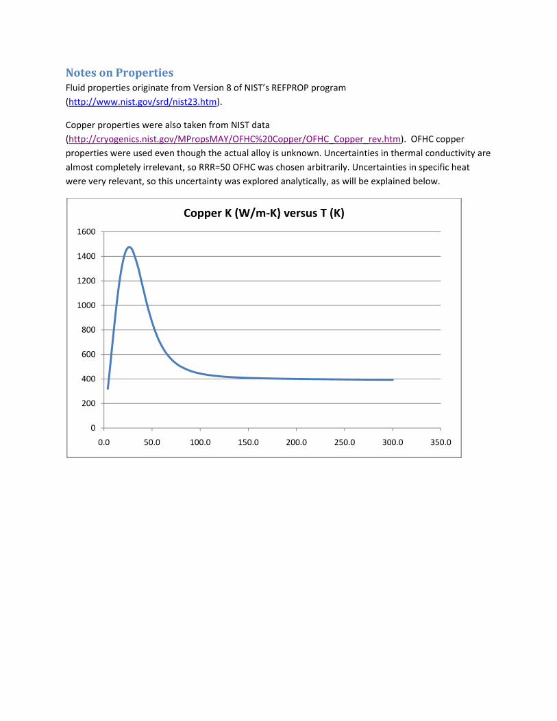
Copper properties were also taken from NIST data (http://cryogenics.nist.gov/MPropsMAY/OFHC%20Copper/OFHC_Copper_rev.htm).  OFHC copper properties were used even though the actual alloy is unknown. Uncertainties in thermal conductivity are almost completely irrelevant, so RRR=50 OFHC was chosen arbitrarily. Uncertainties in specific heat were very relevant, so this uncertainty was explored analytically, as will be explained below. 

 

0

200

400

600

800

1000

1200

1400

1600

0.0 50.0 100.0 150.0 200.0 250.0 300.0 350.0

Copper K (W/m‐K) versus T (K)

 

SINDA/FLUINT Modeling Stagnant (LSTAT=STAG) plena are used to represent both the supply dewar and the ambient exhaust. For the supply dewar, the best‐guess temperature is corrected before the start of a transient if it is higher than saturation, since the inlet plenum (#1000 in the Sinaps models) contains only liquid (whether saturated or subcooled).  

For the outlet plenum (#2000), only its pressure is relevant. Therefore to avoid the need for analyzing mixtures, either 100% nitrogen or 100% hydrogen at atmospheric temperature and pressure is used.  

Similarly, the pipe is assumed to start with room temperature nitrogen or hydrogen instead of air, since the clearing of the initial air in the line is estimated to take less than a second. 

A 20‐segment Sinaps or FloCAD Pipe (SINDA/FLUINT HX macro plus wall model) is used to represent the copper line. The Sinaps diagram is shown at the left below, and the FloCAD diagram (without the pipe wall, and with radiation applied separately using RadCAD rather than explicitly on the diagram as it is in Sinaps) is shown at the right below. 

In a 200 foot (61m) long line that is axially discretized into 20 equal sections, the locations of the thermal wall nodes are at 10, 30, 50 … feet along the line. But the measurement stations are at 40, 80, … feet. To be able to compare test and predictions at the same axial location, the average of two wall nodes is sent to a separate nonphysical node via one‐way conductors, visible as the V‐shapes in the diagrams. This step makes plotting easy, but could be avoided using registers and expressions. For a model with a resolution of 40, there is a one‐to‐one correspondence between node locations and thermocouple locations. 

0

50

100

150

200

250

300

350

400

450

0.0 50.0 100.0 150.0 200.0 250.0 300.0 350.0

Copper Cp (J/kg‐K) versus T (K)

   

The exit paths are set to UPF=1.0 to make sure that the downstream (ambient) state does not affect friction calculation in that last (exit) path. 

The choice of 20 segments can be adjusted by changing both the integer register resol plus editing the Pipe.  A model built with 40 segments produced essentially identical results: the resolution of 20 is therefore adequate. 

Junctions (instantaneous control volumes) can be used within the Pipe instead of time‐dependent tanks, because the residence time of fluid within the line is very small compared to the run times. A model with junctions runs in just a few seconds on a modest PC, whereas one using tanks yields an essentially identical thermal response but costs a minute or two of run time. However, using junctions means that all flow rates along the line are equal at any point in time: the details of a hydrodynamic response are largely lost, and flow cannot go backwards in the inlet (as reported in the NBS report to occur within the first few seconds of some nitrogen runs). Still, the pressure results generated using junctions roughly match those in the NBS report, excepting those first few seconds. 

Note that STUBE connectors (inertia‐less duct elements) are perhaps a better choice than tubes because of the long time scale of interest compared to inertial events, but tubes were employed nonetheless. If tanks were used instead of junctions, tubes would be required in this case because of the strong density gradients. 

Rarely, the choice of tubes and junctions can cause a collision of assumptions: inertia but no mass. Some of the models experienced this collision of assumptions, but only after the quench event was complete. This numerical issue can be seen in the artificial oscillation of pressures in some runs after the line is completely full of liquid. This oscillation does not affect the temperature responses and so was ignored, but it could be removed by replacing the tubes with STUBE connectors. It could also be avoided by using a high‐fidelity model consisting of tanks and tubes, but that step would require longer run times.2 The “collision of assumptions” is described in more detail below. 

The inlet valve has so little resistance that it need not be modeled explicitly: its K‐factor resistance can be added to that of the first path in the Pipe. However, it is added as a separate LOSS connector such that the pressure drop and potential choking could be distinguished if needed. 

Choking was never predicted either at the inlet valve (due to flashing from stagnant, saturated liquid) or at the exhaust, though the Mach numbers at the exhaust were routinely high (about 0.6). 

Correlations, Calibrations, and Variations SINDA/FLUINT’s default set of general‐purpose heat transfer and pressure drop correlations were applied as the baseline. To test their adequacy, scaling factors were applied in the Sinaps‐based models. These scaling factors are initialized to unity, meaning no change from the default value. 

FCmult is a register that is applied to the FCTM factor for flow paths: the turbulent friction factor multiplier for single‐phase flow (and the single‐phase correlations are themselves often used as the basis for two‐phase flow pressure drop).  Therefore, FCmult=1.2 means to augment frictional resistance in the line by about 20%. 

                                                            2  Runtimes of a minute or two might not seem like much, but when such transients are run repeatedly as needed to perform automated correlation to data or to explore statistical sensitivities, they add up. Using junctions and STUBE connectors means a thermal response can be evaluated in a matter of seconds, and a curve fit or statistical result or parametric run can be achieved in minutes. 

UAmult is a register that is applied to the heat transfer tie UAM … the heat transfer conductance multiplier. A value of UAmult=0.8 means to reduce all convective heat transfer coefficients by 20%. 

IDmult is a register applied to the pipe ID in order to assess sensitivity to that dimension. For example, a value of IDmult=1.01 means to increase the pipe inner diameter by 1%. The tolerance on wall thickness for ¾” copper tube is ±0.005” meaning the tolerance on the ID is ±0.01 inches (0.254mm). If this tolerance is interpreted as the limits of a 3‐sigma normal distribution from the nominal (mean) value, 

that means the standard deviation for IDmult is σ = 0.254mm/15.9mm/3 = 0.0053 … a value that will be used to estimate the minimum uncertainty in the cooldown predictions. 

Psupply and Tsupply are the registers defining the temperature (K) and pressure (Pa) of the inlet dewar liquid. Because the state is defined as liquid, Tsupply might be reduced if it is greater than Tsat(Psupply). 

In some models, the critical heat flux (CHF) scaling factors for ties, CHFF, is set using the register CHFfact, 

whose default value is π/24 for the basic CHF correlation described in the SINDA/FLUINT manual. Setting CHFfact to a larger value raises the CHF and prolongs the nucleate boiling regime. Setting it to a negative (‐1.0) signals an alternate CHF correlation, which again scales with the absolute value of CHFF. However, SINDA/FLUINT does not allow nucleate boiling at any flux if the wall temperature is above the thermodynamic critical temperature (Tcrit), as will be discussed in detail later. This restriction limits the importance of the CHF scaling factor in this model or in any cryogenic quenching case, for that matter. 

Setting the integer register oneRun to 1 signals the OPERATIONS logic to make a single transient run. This allows the user to adjust one or more of the above parameters, make a quick run, then refresh the comparison plots to see the effect visually. 

SINDA/FLUINT also can be used to adjust one or more such factors automatically using the Solver high‐level solution module. Setting oneRun = 0 invokes a 20‐step latin hypercube design space scan (DSCANLH), which finds starting points for a Solver‐based curve fit. Both DSCANLH and SOLVER return values of registers such as Psupply, IDmult, etc. that result in the best agreement between test data and predictions based on minimum RMS error. The RMS error is accrued in the OUTPUT block user logic, within initializations and summary calculations performed in the PROCEDURE block.3 

In some cases, oneRun=2 signals that a statistical sampling is to be made to estimate the uncertainty in predictions based on declared probabilities of input parameters (such as IDmult). 

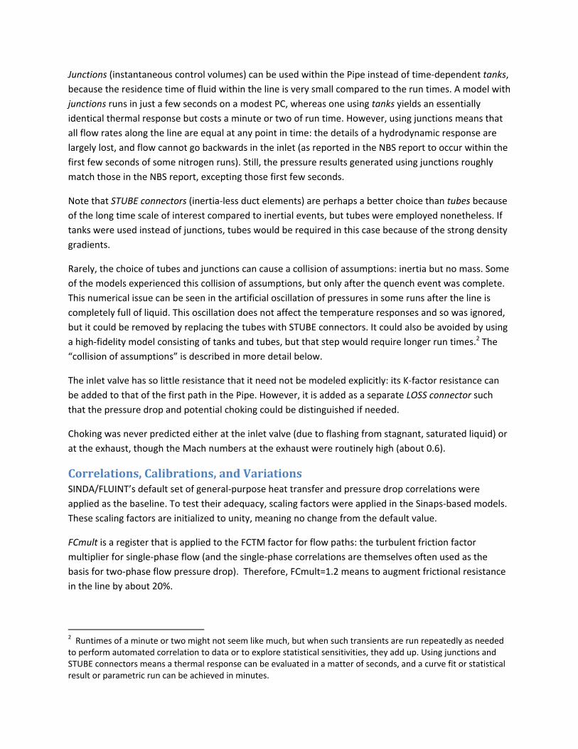
Baseline Hydrogen Comparisons Raw (uncorrected) predictions are compared with the data from NBS Figures 2 through 7 in the plots below. Each page is arranged with predictions for both normal hydrogen (3:1 ortho:para) and parahydrogen on the same page to assist in visual comparison. A discussion follows the charts. 

                                                            3 The hydrogen models use all four stations, but station 2 is skipped in the RMS calculation for nitrogen because of its unpredictable behavior. Station 3 could similarly have been skipped, leaving station 1 and 4 results to form the basis of a best fit, but has been retained in the current versions. Possible causes for the discrepancies in station 2 and 3 data for the nitrogen tests are discussed later. 

 

 

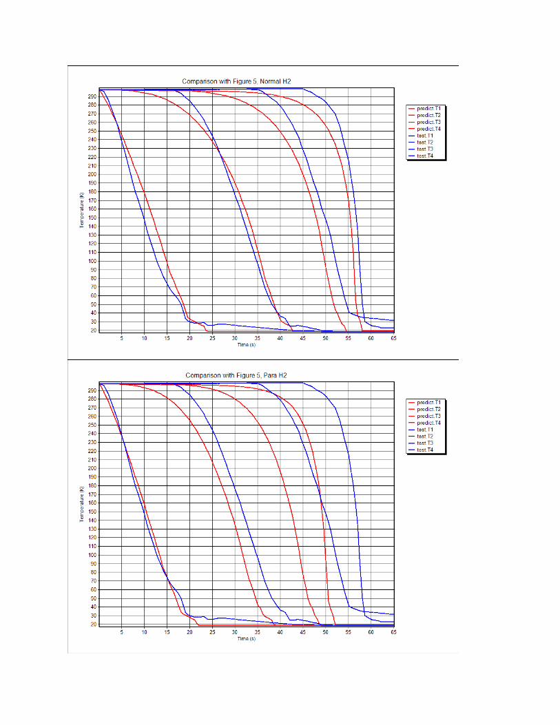
Discussion of Hydrogen Comparisons The predictions made using the baseline (default) correlations in SINDA/FLUINT are quite good for normal hydrogen, especially considering the magnitude of the uncertainties involved (as will be quantified below).  

The final (liquid) temperatures do not always correspond well, especially for the Figure 2 and 6 cases. The NBS test traces appear to be above saturation temperature. There is no single definitive explanation for this discrepancy. Several possibilities include (1) error in the thermocouples at low temperatures, (2) extrapolations made in digitizing the graphs to satisfy the need for temperature data at all times (this is certainly a possibility for Figure 2), (3) similar extrapolations made by the NBS authors when drawing lines, (4) the presence of dissolved gases, or (5) inaccuracies in the reported dewar pressures. Whatever the explanation, the difference is not significant since little energy exchange is involved by the time liquid is present: the cooldown event is over by that time. 

The results for normal hydrogen tend to slightly overpredict the cooldown times. The predictions made using parahydrogen are also adequate, but tend to underpredict the cooldown time. An important observation is that the test results are almost always bracketed between the parahydrogen and normal hydrogen predictions.4 

How far off are the parahydrogen predictions? One way to assess this discrepancy is to adjust one or more of the uncertainty parameters (registers UAmult, CAPmult, FCmult, IDmult, or Psupply). The automation of this process is discussed later, along with means of adjusting multiple uncertainties simultaneously. The discussion of why UAmult turns out to be a poor choice is also deferred. For now, note that any of the individual adjustments in the uncertainties yields good predictions for parahydrogen. Using Figure 5 as a test case, the approximate adjustments in any single parameter required in parahydrogen predictions in order to fit the test data are as follows: 

  CAPmult = 1.2 (20% increase in copper specific heat)   FCmult = 1.4 (40% increase in frictional pressure drop)   IDmult = 0.975 (2.5% decrease in pipe ID)   Psupply reduced from 5.9 atm to 5.0 atm (18% decrease) 

A more thorough analysis of the uncertainties and their relative importance and likelihood is provided later. For now, the key question is:  

Was the hydrogen used in the NBS tests normal hydrogen, and therefore the SINDA/FLUINT predictions are very good, or was it parahydrogen and therefore the predictions made using default correlations are non‐conservative by roughly 20%? 

To understand why there is so much difference between para and normal hydrogen predictions, it must first be understood that vapor phase advection is the dominant phenomenon in this comparison.  Two‐

                                                            4 If the goal of an analysis is to conservatively predict the cooldown time, or the amount of hydrogen that will be consumed in the process, then normal hydrogen should be used as the working fluid. 

phase flow and heat transfer might at first seem to be the most important phenomena, but they turn out to be of secondary importance, especially for hydrogen. 

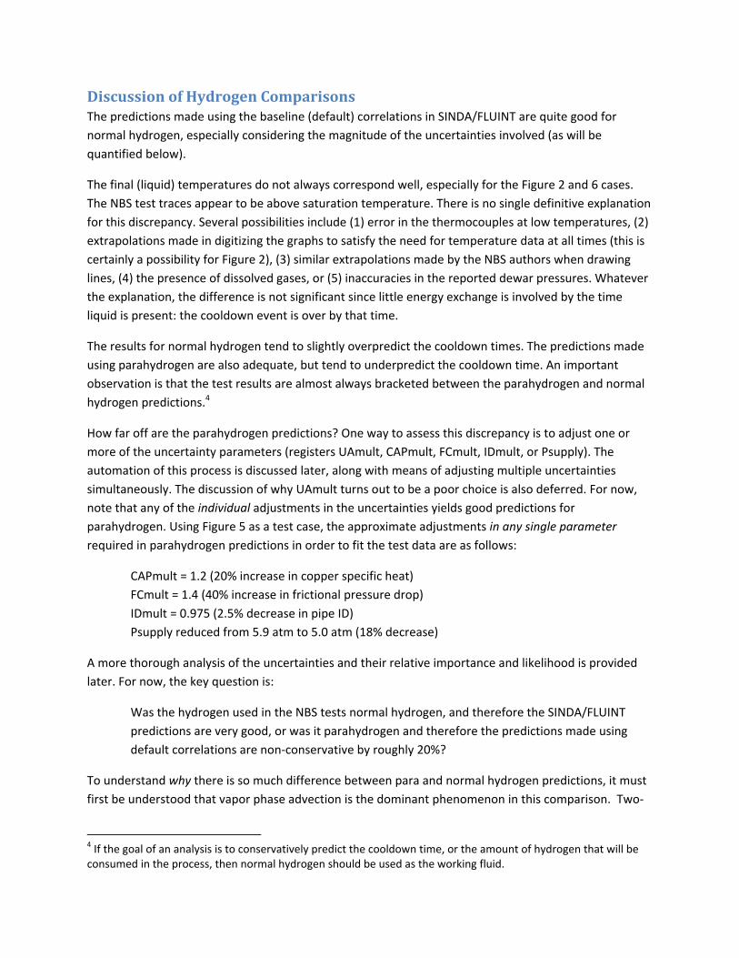
The Importance of the Vapor Phase The importance of vapor phase heat transfer can be readily seen in Figure 9 of the NBS report, which for convenience has been inserted below. This test run was made starting with room temperature pipe in the upstream section (stations 1 and 2), but precooling the pipe in the downstream section (stations 3 and 4).5 Notice that the temperatures of stations 3 and 4 rise back up to nearly room temperature in just a few seconds (with the warmer upstream pipe being the source of heating), then those wall temperatures fall back down as cold vapor enters those sections. In many ways, it is better to think of the liquid hydrogen as a source of cold vapor than to think of it as quenching the pipe. 

 

These statements can also be backed up by analytic arguments. 

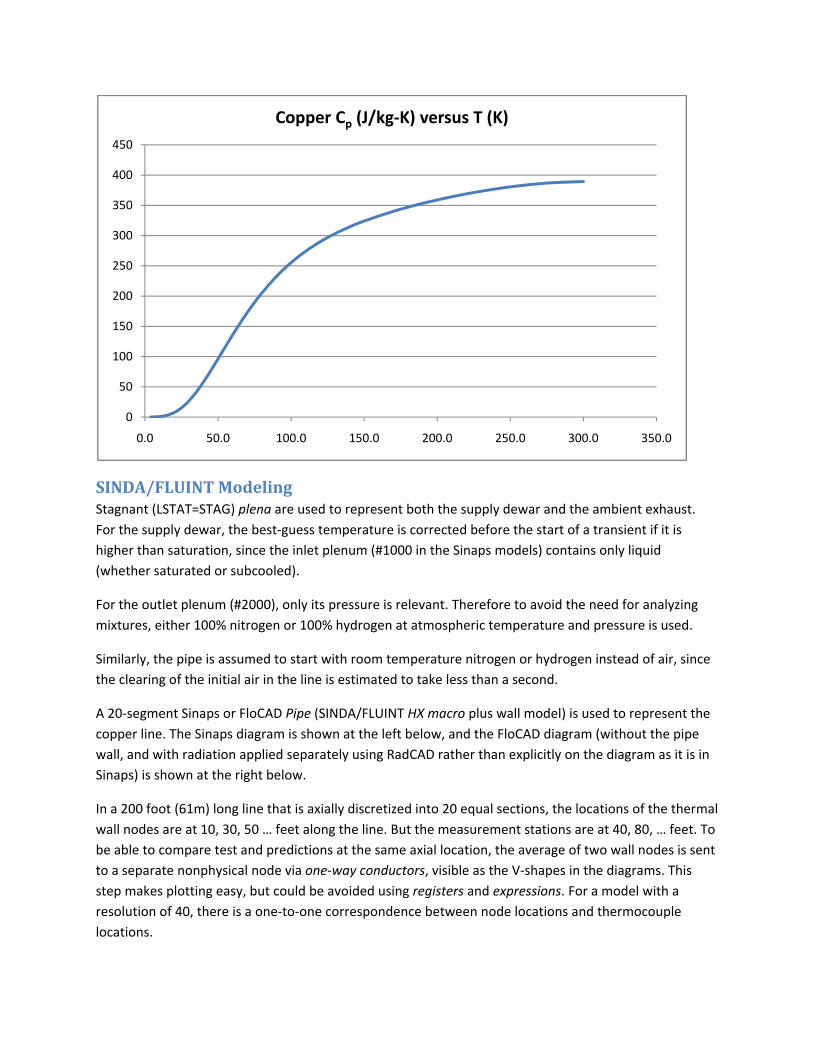
First, note that the Cp of copper (the previously presented figure is reprised below for convenience) drops off sharply once it is below 100K. What this means is that essentially all of the enthalpy of the copper has been removed in the process of cooling it from 300K to 100K, and that comparatively little 

                                                            5 This case could not be used for analytic comparisons since the initial condition (the temperature of the pipe in between stations) was unknown. 

energy is extracted below 100K. In other words, the vapor does the bulk of the cooling job long before liquid appears next to the pipe wall. 

 

Almost all the pressure drop in the pipe happens in the vapor section, which is no surprise given the low density of that phase. Liquid at relatively low velocity must be accelerated up to a very fast vapor velocity; the mass flow of liquid at the inlet roughly matches the exit mass flow of vapor, yet the volumetric flows are different by orders of magnitude.  In each run, the mass flow rate starts small, and grows quickly as the “plug” of high‐friction vapor shrinks. This difference in relative frictional resistance is paralleled (per Reynolds’ Analogy) by a similar difference in heat transfer coefficient between vapor and liquid regions. Of course, there are also huge temperature differences between wall and fluid in the vapor region compared to the liquid region (because the pipe has already been nearly completely quenched by the time liquid can be sustained within it). 

Finally, from a hydrogen thermodynamic perspective, note the relatively large Cp of hydrogen gas compared to other fluids. For parahydrogen, the isobaric enthalpy drop from 300K to 30K (at about 0.8MPa, the saturation pressure corresponding to 30K) is 4015 kJ/kg, compared to a heat of vaporization at 30K of about 291 kJ/kg. This difference means that sensible cooling is 4015/291=13.8 times more important than is latent cooling. 

Given the importance of vapor phase cooling of the line, the difference in properties between gaseous para and normal hydrogen are explored next. 

0

50

100

150

200

250

300

350

400

450

0.0 50.0 100.0 150.0 200.0 250.0 300.0 350.0

Copper Cp (J/kg‐K) versus T (K)

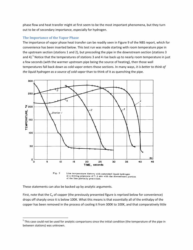
The Key Differences between Para and Ortho Hydrogen At 2 bar,6 the thermal conductivity (W/m‐K) of gaseous hydrogen in the normal and para states is shown in the graph below. 

 

From 150K to 200K, parahydrogen is almost 26% more conductive than is normal hydrogen. 

The specific heat (J/kg‐K) shows an even stronger variation between the two forms of hydrogen (please note that the graph below does not start at zero Cp on the Y axis). 

                                                            6 The relevant vapor properties are insensitive to pressure. 2 bar was chosen as representative. 

0

0.05

0.1

0.15

0.2

0.25

0 50 100 150 200 250 300 350

Para H2Normal H2

 

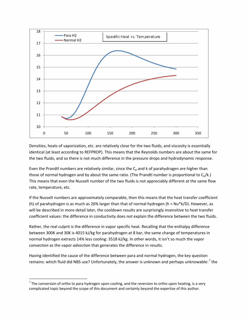
Densities, heats of vaporization, etc. are relatively close for the two fluids, and viscosity is essentially identical (at least according to REFPROP). This means that the Reynolds numbers are about the same for the two fluids, and so there is not much difference in the pressure drops and hydrodynamic response. 

Even the Prandtl numbers are relatively similar, since the Cp and k of parahydrogen are higher than those of normal hydrogen and by about the same ratio. (The Prandtl number is proportional to Cp/k.) This means that even the Nusselt number of the two fluids is not appreciably different at the same flow rate, temperature, etc. 

If the Nusselt numbers are approximately comparable, then this means that the heat transfer coefficient (h) of parahydrogen is as much as 26% larger than that of normal hydrogen (h = Nu*k/D). However, as will be described in more detail later, the cooldown results are surprisingly insensitive to heat transfer coefficient values: the difference in conductivity does not explain the difference between the two fluids. 

Rather, the real culprit is the difference in vapor specific heat. Recalling that the enthalpy difference between 300K and 30K is 4015 kJ/kg for parahydrogen at 8 bar, the same change of temperatures in normal hydrogen extracts 14% less cooling: 3518 kJ/kg. In other words, it isn’t so much the vapor convection as the vapor advection that generates the difference in results. 

Having identified the cause of the difference between para and normal hydrogen, the key question remains: which fluid did NBS use? Unfortunately, the answer is unknown and perhaps unknowable: 7 the 

                                                            7 The conversion of ortho to para hydrogen upon cooling, and the reversion to ortho upon heating, is a very complicated topic beyond the scope of this document and certainly beyond the expertise of this author. 

10

11

12

13

14

15

16

17

18

0 50 100 150 200 250 300 350

Para H2Normal H2

NBS authors likely did not know, and in fact the exact concentration of para and ortho may have changed between tests. 

Note that REFPROP does not provide pure ortho hydrogen properties, nor other combinations of ortho and para other than 3:1 “normal” hydrogen. Thus, only two distinct mixtures of para and ortho hydrogen were available to use to generate comparison predictions. 

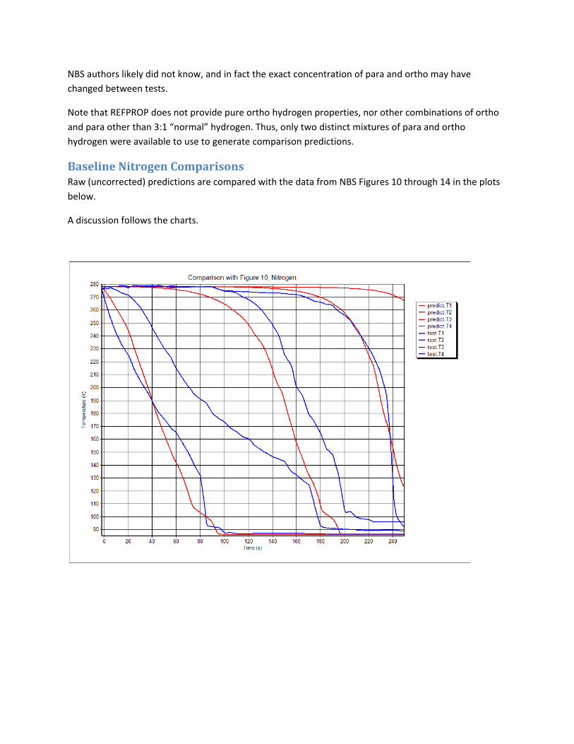
Baseline Nitrogen Comparisons Raw (uncorrected) predictions are compared with the data from NBS Figures 10 through 14 in the plots below. 

A discussion follows the charts. 

 

 

 

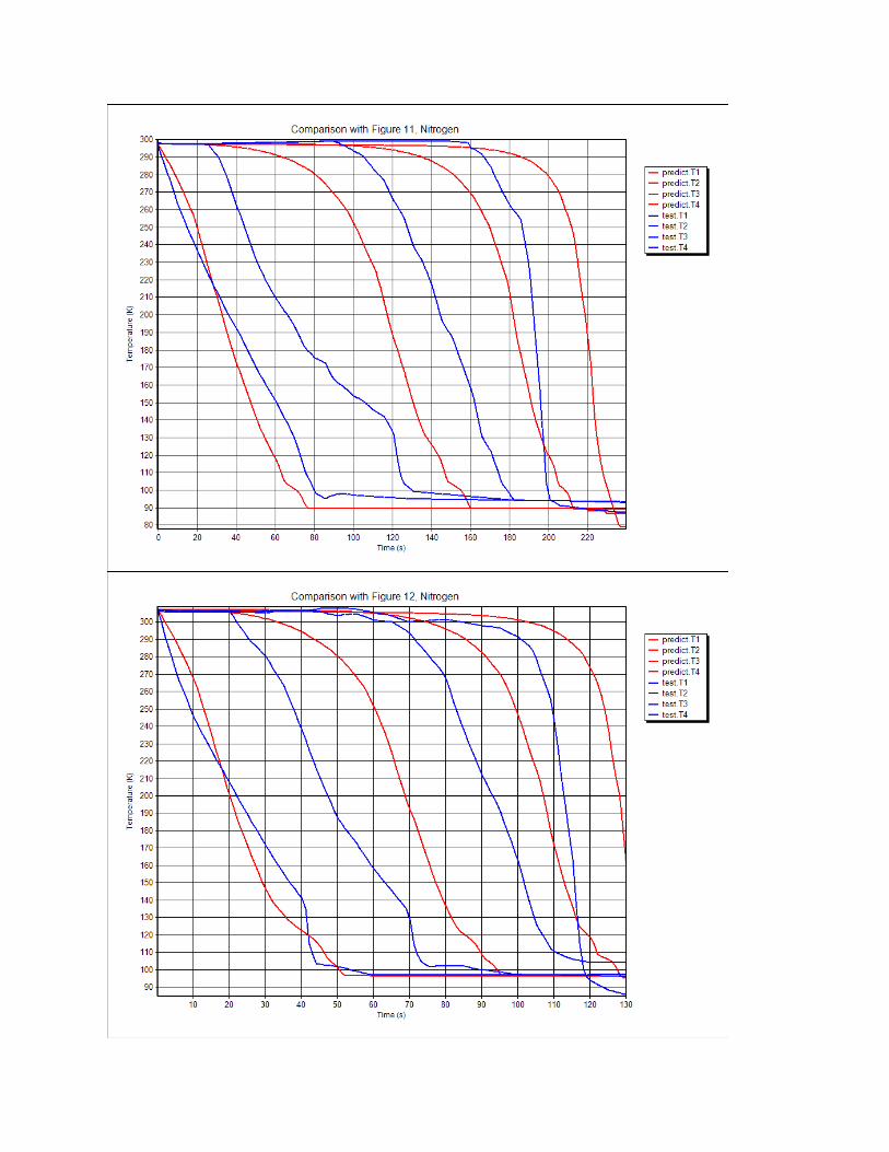
Discussion of Nitrogen Comparisons Despite the smaller temperature range traversed, the comparisons between test and predictions made using default correlations are worse for nitrogen than they were for normal hydrogen. However, the quality of the predictions is better than it was for parahydrogen, and the nitrogen predictions also are at least in the “right direction” (i.e., on the conservative side). 

Using Figure 12 as a test case, the same type of preliminary adjustment of individual uncertainties made for the Figure 5 hydrogen case can be repeated to gain a measure of how far off the predictions are. The following is a list of individual adjustments on each uncertainty as required to bring the nitrogen predictions in line with test data: 

  CAPmult = 0.9 (10% decrease in copper specific heat)   FCmult = 0.8 (20% decrease in frictional pressure drop)   IDmult = 1.02 (2% increase in pipe ID)   Psupply increased from 5.9 atm to 6.5 atm (11% increase) 

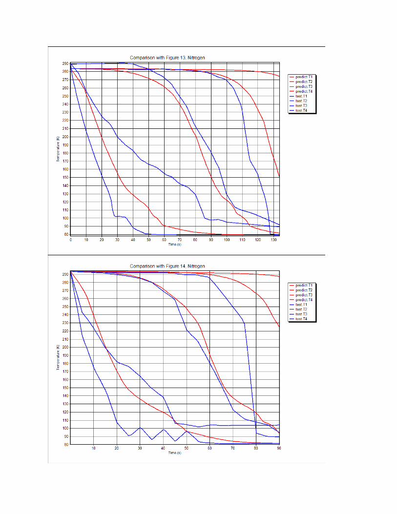
It appears SINDA/FLUINT is roughly 10% conservative in the prediction of nitrogen cooldown. The discrepancy appears to be even higher for subcooled cases (Figures 13 and 14 in the NBS report). 

While it doesn’t take a large adjustment to yield good results for both stations 1 and 4, stations 2 and 3 do not appear so well‐behaved. Station 2 in particular has a very different characteristic from other stations, and from how it behaved during hydrogen testing. It begins to cool down very quickly (almost instantly), and then cools slower than the other stations. While it might be easy to dismiss this behavior as evidence of an aberrant thermocouple, there might be a physical explanation.  

The NBS report was focused not on cooldown times (thermal responses) but rather on pressure events. Its authors report that, unlike hydrogen, nitrogen peak pressures were sensitive to subcooling versus saturation. More to the point, they report that peak surge pressures were sometimes experienced at station 2, whereas with hydrogen the peak pressure was always experienced at station 1. This peak happens in the first few seconds, however: much shorter than the time scale of the thermal cooldown event. 

One possible explanation is that a core of liquid nitrogen initially shoots past station 1, insulated by a low conductivity gas (inverted annular flow) due to film boiling. In other words, for hydrogen there was more of a flat front of liquid progressing through the pipe, whereas with nitrogen there was an extended two‐phase zone. 

SINDA/FLUINT does not currently8 support an inverted annular flow regime for hydrodynamic characterization, but it does include the effects of this regime on heat transfer. In the current study, homogeneous (no slip) flow was assumed in addition to thermodynamic equilibrium (perfect mixing at each axial location). To truly analyze a suspended liquid core would require not only an inverted annular regime to be added to the code, but also a full two‐fluid model using “twinned tanks, twinned tubes, 

                                                            8 The current production release is Version 5.2. 

and twinned ties:” slip flow with phasic nonequilibrium. Because of the short time scales of the thermohydraulic events that are exposed in such high‐temporal‐fidelity modeling, the CPU costs of such a run would be very high, and a new level of uncertainties would be unveiled (see SINDA/FLUINT User’s Manual and training notes for more details). The engineering value of this investigation is questionable since the temperatures of both stations 1 and 4 are still very amenable to analysis using simpler, faster methods, and prediction of station 4 temperatures is the key to estimating cooldown times. Therefore, the idea of a floating core of liquid nitrogen was not investigated analytically in this study. 

Distinct inflection points can be seen in the temperature histories for the nitrogen tests as the stations cross below about 140K: the rate of cooling suddenly increases. This change in slope is especially evident in the test data for stations 1 and 2 in Figure 12. It is believed that these points represent the conversion from film boiling to transition boiling. (Further transitions to full nucleate boiling should occur at even colder temperatures, but the evidence for those changes is more tenuous.)  

One of the subpurposes of this study was to seek such points, since SINDA/FLUINT’s default methods do not allow transition or nucleate boiling to commence until the wall is at least few degrees below the critical point such that it can thermodynamically sustain liquid.9 For N2, whose critical point is 126K, this means liquid is not permitted against the wall until the wall is cooler than about 120K. However, in reality, as liquid droplets penetrate closer and closer to the wall, heat transfer is likely to increase during this brief regime. In other words, despite the lack of available correlations, a “transition” between film boiling and transition or nucleate boiling happens just above the critical point. (The “transition into transition boiling” is less evident in hydrogen traces, but does appear to sometimes happen in the 30K‐40K range: again just above the thermodynamic critical point instead of just below it.)  

Nonetheless, the final results are very insensitive to this effect. Changing the heat transfer coefficient or CHF (critical heat flux) cut‐off does very little to the final results. In other words, while there does appear to be some phenomenological gap in the SINDA/FLUINT default correlation set, its absence has little relevance to this type of cooldown problem. One explanation for the insensitivity of the predictions to any details of two‐phase heat transfer is the relative unimportance of two‐phase heat transfer compared to single‐phase vapor heat transfer, which has been discussed previously (see prior hydrogen discussion, as well as a more detailed explanation below). In other words, the major effect of an extended two‐phase zone in the nitrogen tests is that it caused colder vapor to be injected farther into the pipe. 

However, the argument for the relative importance of vapor phase advection over two‐phase advection is not as strong for nitrogen as it is for hydrogen. For example, the enthalpy change going from 300K to 100K (again, at about 8 bar) is 222 kJ/kg for nitrogen, versus a heat of vaporization of 161 kJ/kg: single‐phase vapor heat transfer is only slightly (222/161=1.38 times) more important than two‐phase heat transfer for nitrogen.  (This is perhaps why an inverted annular regime may have formed in nitrogen but not in hydrogen … or at least not as noticeably in hydrogen. For nitrogen, cooling by latent heat is comparatively much more important than when quenching using hydrogen.) 

                                                            9 See Section 3.6.7 of the SINDA/FLUINT Manual regarding advanced two‐phase options for heat transfer ties. 

It should be noted that, in an attempt to improve the predictions, other SINDA/FLUINT options were tested that are normally appropriate to strongly varying gradients in single‐phase flow. The integrated property method for heat transfer ties (MODR=5) was applied, but had no significant effect.10 Similarly, a correction for friction for large radial temperature gradients (FCPVAR) did not have a significant effect. 

Calibrating for Best Fit In the prior section, several uncertainties were individually adjusted to improve the correspondence between test and predictions: in order to help quantify the accuracy of the predictions. In this section, several of them11 will be adjusted simultaneously using SINDA/FLUINT’s Solver module.12 

For the Solver to work, it must minimize or maximize the objective (a variable named OBJECT), perhaps subject to one or more constraints. No constraints were applicable in this case. The objective was chosen to be the RMS (root‐mean‐square) error, which is calculated in OUTPUT CALLS at discrete intervals: 

  OBJECT = SQRT{Σi=1,n(Ti – Pi)2)/n} 

The difference between test (Ti) and predictions (Pi) excluded station 2 for nitrogen because of the unpredictable response of that trace. Initialization (zeroing) and final calculations (e.g., taking the square root) take place in PROCEDURE before and after the transient call. The Solver evaluation PROCEDURE is repeated iteratively: a Solver calibration run requires roughly 50 transients be executed, each testing different values of the uncertainty parameters or “design variables.” 

CAPmult, FCmult, and Psupply were all chosen as design variables, with limits placed on their range of possible values. These limits allowed a pre‐scan to be used: DSCANLH, which returns a starting point for the Solver, which then completes the minimization. Using Figure 12 (saturated nitrogen) again as a demonstration case, the following fit was found: 

  CAPmult = 0.986 (1.4% decrease in copper specific heat)   FCmult = 0.87 (13% decrease in frictional pressure drop)   Psupply increased from 5.9 atm to 6.1 atm (3.3% increase) 

Of course, when all three parameters are adjusted together, much smaller changes are needed to achieve the same fit versus adjusting only a single parameter at a time.  The above results were typical: little adjustment was needed in the CAPmult, whereas moderate adjustment was needed in FCmult and/or Psupply. In other words, the copper properties are unlikely to be a source of error, but the pressure measurements might be in slight error and the pressure drop calculations probably contain the most error. 

                                                            10 In retrospect, this is not surprising given the insensitivity to UAmult, as documented below. 11 IDmult, the inner diameter multiplier, will be excluded from this list. The sensitivity to this manufacturing tolerance will be investigated in the subsequent section using different methods. 12 Officially a “nonlinear programming system,” the Solver may be used for design optimization, worst‐case scenario seeking, and‐‐as used here‐‐automating the fitting of models to data. 

The ID was assumed perfectly accurate (IDmult = 1.0) in the above assessment such that the effect of the manufacturing tolerance for that parameter could be assessed independently using statistical methods (see below).  Also, the heat transfer multiplier UAmult was also excluded from the list of curve fit parameters, but for a very different reason as explained in a later subsection: adjustments in that parameter are largely irrelevant. 

The plot of the fitted response corresponding to the above numbers is presented below, along with a reprise of the original (uncorrected) predictions (corresponding to Psupply=5.9 atm, and CAPmult=1.0 and FCmult=1.0). 

Note that, in the ideal case, all possible uncertainties would be combined into a single calibration: they would all be added as “design variables.” Similarly, all available data (e.g., Figures 2 through 7 for hydrogen, Figures 10 through 14 for nitrogen) would be used simultaneously as a measure of best fit: a series of transients would be used in PROCEDURE to calculate a single RMS error accumulated over all of the pertinent runs. 

 

Baseline (uncorrected) 

Correlated

The Insensitivity to Heat Transfer Coefficient One of the surprises of this study was the relative insensitivity of the results to changes in UAmult: the heat transfer multiplier. UAmult was applied to all heat transfer: liquid, vapor, and two‐phase. In other words, despite the dominance of vapor phase advection, raising or lowering heat transfer rates did not greatly affect the predicted wall temperatures. 

The reason for this insensitivity is that the effect is self‐correcting. If heat transfer rates are raised, then the liquid will tend to reach the same place in the pipe sooner. This means the vapor generation rate would be higher. But if the vapor generation rate is higher, then the frictional resistance is also higher: the same pressure drop between the dewar and the environment drives less flow through the tube. Specifically, raising UAmult does not significantly decrease the cooldown time since the mass flow rate through the tube remains largely unaffected. Instead, all that happens is that the temperature profiles in the vapor portion of the tube change, and even then only modestly. 

Similarly, changing just the two‐phase coefficients such as CHFF had little to no effect (as noted earlier). 

This lack of sensitivity to heat transfer calculations was somewhat disappointing, since one of the subpurposes of this study was to evaluate the default correlations in SINDA/FLUINT for heat transfer. However, this effect is at least encouraging that the predictions appear to be insensitive to any heat transfer uncertainties, though this is certainly not a global conclusion (e.g., it might not be applicable to an analysis of a turbopump cooldown case). 

Estimate of the Minimum Uncertainty in Predictions The uncertainty in the inner diameter (ID) of the tube was excluded from the prior multivariate calibration of other uncertainties such that it could be independently assessed. The uncertainty in Psupply is caused by measurement accuracy (as well as unknown changes to the pressure during dewar depletion). The uncertainty in CAPmult is due to the lack of specific knowledge of the copper alloy used. The uncertainty in UAmult and FCmult are due to the accuracy and appropriateness of the underlying heat transfer and pressure drop correlations. 

But while the uncertainty in IDmult is partly due measurement accuracy (the exact pipe specifications being unknown), it is mostly assumed to be a function of manufacturing tolerance: IDmult = 1.0000±(3*0.0053) as described previously. Therefore, unlike the other unknowns, the degree to which IDmult is uncertain can be quantified, so it is treated separately13 using statistical techniques. 

The starting point for this statistical check is chosen as the results of the Solver‐generated curve fit for Figure 12, with CAPmult=0.986, FCmult=0.87 and Psupply=6.1 atm.  This case will be sampled for the sensitivity of the cooldown time (defined as the time to bring the station 4 temperature down to Tsupply) and the quantity of liquid nitrogen used to accomplish this task.  

                                                            13 This separation is largely for demonstration purposes and does not represent any limitation in SINDA/FLUINT. In other words, all uncertainties could be adjusted simultaneously using the Solver to achieve a best fit, or all of them could be assessed using DSAMPLE or other reliability engineering methods to predict the overall accuracy of the predictions … at least if the uncertainty in each variable could be estimated. 

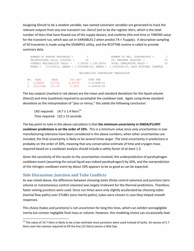
Assigning IDmult to be a random variable, two named constraint variables are generated to track the relevant outputs from any one transient run: liters2 (set to be the register liters, which is the total number of liters that have flowed out of the supply dewar), and cooltime (the end time or TIMEND value for the transient run, which was set in VARIABLES 2 when predict.T4 < Tsupply).  A descriptive sampling of 50 transients is made using the DSAMPLE utility, and the RCSTTAB routine is called to provide summary data. 

NUMBER OF RANDOM VARIABLES = 1 NUMBER OF REL. CONSTRAINTS = 2 RELPROCEDURE CALLS (LOOPCR) = 50 VS. MAXIMUM (NLOOPR) = 50 OVERALL RELIABILITY TALLY = 1.00000 ( 100.000%) TOTAL CUMULATIVE CALLS = 50 NSEED = 111319312, AERRR = 1.000000E-05, RERRR = 1.000000E-03, LAST ROUTINE: DSAMPLE

RELIABILITY CONSTRAINT TABULATION

NO. NAME MEAN STD DEV COEF VAR 1 LITERS2 14.714 0.47274 3.21284E-02 2 COOLTIME 121.59 5.0941 4.18947E-02

The key outputs (marked in red above) are the mean and standard deviations for the liquid volume (liters2) and time (cooltime) required to accomplish the cooldown task.  Again using three standard deviations as the interpretation of “plus or minus,” this yields the following conclusion: 

  LN2 required:  14.7 ± 1.4 liters14   Time required:  122 ± 15 seconds 

The key point to note in the above calculation is that the minimum uncertainty in SINDA/FLUINT cooldown predictions is on the order of 10%.  This is a minimum value since only uncertainties in one manufacturing tolerance have been considered in the above numbers; when other uncertainties are included, the final uncertainty is likely to be several times larger. The total uncertainty in predictions is probably on the order of 30%, meaning that any conservative estimate of time and cryogen mass required based on a cooldown analysis should include a safety factor of at least 1.3. 

Given the sensitivity of the results to the uncertainties involved, the underprediction of parahydrogen cooldown event (assuming the actual liquid was indeed parahydrogen!) by 20%, and the overprediction of the nitrogen cooldown event by about 10% appears to be as good as can be expected. 

Side Discussion: Junction and Tube Conflicts As was noted above, the difference between choosing tanks (finite control volumes) and junctions (zero volume or instantaneous control volumes) was largely irrelevant for the thermal predictions. Therefore, faster solving junctions were used. Since run times were only slightly accelerated by choosing tubes (inertial flow paths) over STUBEs (zero inertia paths), tubes were chosen in case they helped smooth responses. 

This choice (tubes and junctions) is not uncommon for long thin lines, which can exhibit nonnegligible inertia but contain negligible fluid mass or volume. However, this modeling choice can occasionally lead 

                                                            14 The value of 14.7 liters is likely to be a low estimate since junctions were used instead of tanks. An excess of 2.7 liters over the volume required to fill the line (12 liters) seems a little low. 

to an interesting conflict of assumptions that, if experienced, becomes evident late in the simulations. After the pipe has been quenched, the vapor “plug” is absent and very high flow rates emerge (at which point the NBS team stopped the run). At this point, if the analysis continues, the pipe contains a fast‐moving stream of flashing low‐quality liquid with relatively high inertia but low flow resistance.  

At this point, the junctions and tubes get into a rare numerical battle, oscillating between a low‐quality or all‐liquid state and a high‐quality or all‐vapor state (with large resistance and even choking). These answers are spurious. The “fight” disappears if either the junctions are switched to tanks (high‐fidelity modeling), or if the tubes are switched to STUBEs (low‐fidelity or quasi‐steady modeling). Otherwise, when the instantaneously‐changing thermodynamic states of low‐fidelity junctions are combined with high‐fidelity inertial tubes, and when the thermodynamic state is such a delicate function of pressure, the artificial oscillation in pipe states and flow rates can emerge. 

In a production model, tubes would have been dropped in favor of STUBEs to avoid this artificial issue. However, since this is a demonstration case, it was decided to leave the tubes present to allow the topic to be discussed. 

Conclusions For the case considered of a plain tube being quenched by a liquid cryogen, the default methods available in SINDA/FLUINT have been found to be adequate considering the uncertainties involved.  

A safety factor of at least 1.3 should be applied to predicted times and cryogen quantities. It is recommended that the size of uncertainties be investigated in any real engineering problem (perhaps using some of the methods demonstrated in this study), such that an appropriately conservative safety factor can be applied. 

There is evidence that SINDA/FLUINT tends to underestimate the heat transfer when the wall temperature is in the range 0.95*Tcrit to 1.1*Tcrit, but there is little benefit to seeking an improved correlation due to the insensitivity of the predictions to any adjustments in heat transfer coefficients. SINDA/FLUINT users can always override the default correlations set as needed.