COMPARISON THEOREMS FOR CONJUGATE POINTS IN

SUB-RIEMANNIAN GEOMETRY

D. BARILARI1 AND L. RIZZI2

Abstract. We prove sectional and Ricci-type comparison theorems for the existence of con-jugate points along sub-Riemannian geodesics. In order to do that, we regard sub-Riemannianstructures as a special kind of variational problems. In this setting, we identify a class ofmodels, namely linear quadratic optimal control systems, that play the role of the constantcurvature spaces. As an application, we prove a version of sub-Riemannian Bonnet-Myers the-orem and we obtain some new results on conjugate points for three dimensional left-invariantsub-Riemannian structures.

Contents

1. Introduction 21.1. Related literature 51.2. Structure of the paper 62. Preliminaries 62.1. Minimizers and geodesics 72.2. Geodesic flag and Young diagram 83. Jacobi fields revisited: conjugate points and Riccati equation 93.1. Riemannian interlude 103.2. Canonical frame 113.3. Linearized Hamiltonian 133.4. Riccati equation: blow-up time and conjugate time 144. Microlocal comparison theorem 154.1. LQ optimal control problems 154.2. Constant curvature models 164.3. General microlocal comparison theorem 185. Average microlocal comparison theorem 196. A sub-Riemannian Bonnet-Myers theorem 237. Applications to left-invariant structures on 3D unimodular Lie groups 247.1. Invariants of a 3D contact structure 257.2. Left-invariant structures 26Appendix A. Comparison theorems for the matrix Riccati equation 28A.1. Well posedness of limit Cauchy problem 29Appendix B. Proof of Lemma 32 30Appendix C. Proof of Proposition 14 and Lemma 15 30References 32

1Universite Paris Diderot - Paris 7, Institut de Mathematique de Jussieu, UMR CNRS 7586 -UFR de Mathematiques

2CNRS, CMAP Ecole Polytechnique and Equipe INRIA GECO Saclay Ile-de-France, Paris,France

E-mail addresses: davide.barilari@imj-prg.fr, luca.rizzi@cmap.polytechnique.fr.Date: May 13, 2016.2010 Mathematics Subject Classification. 53C17, 53C21, 53C22, 49N10.Key words and phrases. sub-Riemannian geometry, Curvature, comparison theorems, conjugate points.

1

1. Introduction

Among the most celebrated results in Riemannian geometry, comparison theorems play aprominent role. These theorems allow to estimate properties of a manifold under investigationwith the same property on the model spaces which, in the classical setting, are the simplyconnected manifolds with constant sectional curvature (the sphere, the Euclidean plane andthe hyperbolic plane). The properties that may be investigated with these techniques arecountless and include, among the others, the number of conjugate points along a given geodesic,the topology of loop spaces, the behaviour of volume of sets under homotheties, Laplaciancomparison theorems, estimates for solutions of PDEs on the manifold, etc.

In this paper we are concerned, in particular, with results of the following type. Until furthernotice, M is a Riemannian manifold, endowed with the Levi-Civita connection, Sec(v, w) is thesectional curvature of the plane generated by v, w ∈ TxM .

Theorem 1. Let γ(t) be a unit-speed geodesic on M . If for all t ≥ 0 and for all v ∈ Tγ(t)M

orthogonal to γ(t) with unit norm Sec(γ(t), v) ≥ k > 0, then there exists 0 < tc ≤ π/√k such

that γ(tc) is conjugate with γ(0).

Notice that the quadratic form Sec(γ(t), ·) : Tγ(t)M → R, which we call directional curvature(in the direction of γ), computes the sectional curvature of the planes containing γ. Theorem 1compares the distance of the first conjugate point along γ with the same property computedon the sphere with sectional curvature k > 0, provided that the directional curvature along thegeodesic on the reference manifold is bounded from below by k. Theorem 1 also contains allthe basic ingredients of a comparison-type result:

• A micro-local condition, i.e. “along the geodesic”, usually given in terms of curvature-type quantities, such as the sectional or Ricci curvature.• Models for comparison, that is spaces in which the property under investigation can be

computed explicitly.

As it is well known, Theorem 1 can be improved by replacing the bound on the directional cur-vature with a bound on the average, or Ricci curvature. Moreover, Theorem 1 leads immediatelyto the celebrated Bonnet-Myers theorem (see [25]).

Theorem 2. Let M be a connected, complete Riemannian manifold, such that, for any unit-speed geodesic γ(t), the Ricci curvature Ric∇(γ(t)) ≥ nk. Then, if k > 0, M is compact, hasdiameter non greater than π/

√κ and its fundamental group is finite.

In Riemannian geometry, the importance of conjugate points rests on the fact that geodesicscease to be minimizing after the first one. This remains true for strongly normal sub-Riemanniangeodesics. Moreover, conjugate points, both in Riemannian and sub-Riemannian geometry, arealso intertwined with the analytic properties of the underlying structure, for example they affectthe behaviour of the heat kernel (see [12, 13] and references therein).

The main results of this paper are comparison theorems on the existence of conjugate points,valid for any sub-Riemannian structure.

We briefly introduce the concept of sub-Riemannian structure. A sub-Riemannian structureon a manifold M can be defined as a distribution D ⊆ TM of constant rank, with a scalarproduct that, unlike the Riemannian case, is defined only for vectors in D . Under mild assump-tions on D (the Hormander condition) any connected sub-Riemannian manifold is horizontallypath-connected, namely any two points are joined by a path whose tangent vector belongs toD . Thus, a rich theory paralleling the classical Riemannian one can be developed, giving ameaning to the concept of geodesic, as an horizontal curve that locally minimises the length.

Still, since in general there is no canonical completion of the sub-Riemannian metric to aRiemannian one, there is no way to define a connection a la Levi-Civita and thus the familiarRiemannian curvature tensor. The classical theory of Jacobi fields and its connection with thecurvature plays a central role in the proof of many Riemannian comparison results, and thegeneralisation to the sub-Riemannian setting is not straightforward. The Jacobi equation itself,

2

being defined in terms of the covariant derivative, cannot be formalised in the classical sensewhen a connection is not available.

In this paper we focus on results in the spirit of Theorem 1 even tough there are no evidentobstructions to the application of the same techniques, relying on the Riccati equations forsub-Riemannian geodesics, to other comparison results. We anticipate that the comparisonsmodels will be linear quadratic optimal control problems (LQ problems in the following), i.e.minimization problems quite similar to the Riemannian one, where the length is replaced by afunctional defined by a quadratic Lagrangian. More precisely we are interested in admissibletrajectories of a linear control system in Rn, namely curves x : [0, t]→ Rn for which there existsa control u ∈ L2([0, t],Rk) such that

x = Ax+Bu, x(0) = x0, x(t) = x1, x0, x1, t fixed,

that minimize a quadratic functional φt : L2([0, t],Rk)→ R of the form

φt(u) =1

2

∫ t

0(u∗u− x∗Qx) dt.

Here A,B,Q are constant matrices of the appropriate dimension. The symmetric matrix Q isusually referred to as the potential. Notice that it makes sense to speak about conjugate timeof a LQ problem: it is the time tc > 0 at which extremal trajectories lose local optimality, asin (sub)-Riemannian geometry. Moreover, tc does not depend on the data x0, x1, but it is anintrinsic feature of the problem. These kind of structures are well known in the field of optimalcontrol theory, but to our best knowledge this is the first time they are employed as modelspaces for comparison results.

With any ample, equiregular sub-Riemannian geodesic γ(t) (see Definition 11), we associate:its Young diagram D, a scalar product 〈·|·〉γ(t) : Tγ(t)M × Tγ(t)M 7→ R extending the sub-Riemannian one and a quadratic form Rγ(t) : Tγ(t)M 7→ R (the sub-Riemannian directionalcurvature), all depending on the geodesic γ(t). We stress that, for a Riemannian manifold, anynon-trivial geodesic has the same Young diagram, composed by a single column with n = dimMboxes, the scalar product 〈·|·〉γ(t) coincides with the Riemannian one, and Rγ(t)(v) = Sec(v, γ(t)).

In this introduction, when we associate with a geodesic γ(t) its Young diagram D, we im-plicitly assume that γ(t) is ample and equiregular. Notice that these assumptions are true forthe generic geodesic, as we discuss more precisely in Sec. 2.2.

In the spirit of Theorem 1, assume that the sub-Riemannian directional curvature is boundedfrom below by a quadratic form Q. Then, we associate a model LQ problem (i.e. matrices A andB, depending on γ) which, roughly speaking, represents the linearisation of the sub-Riemannianstructure along γ itself, with potential Q. We dub this model space LQ(D;Q), where D is theYoung diagram of γ, and Q represents the bound on the sub-Riemannian directional curvature.The first of our results can be stated as follows (see Theorem 24).

Theorem 3 (sub-Riemannian comparison). Let γ(t) be a sub-Riemannian geodesic, with Youngdiagram D, such that Rγ(t) ≥ Q+ for all t ≥ 0. Then the first conjugate point along γ(t) occursat a time t not greater than the first conjugate time of the model LQ(D;Q+). Similarly, ifRγ(t) ≤ Q− for all t ≥ 0, the first conjugate point along γ(t) occurs at a time t not smaller thanthe first conjugate time of LQ(D;Q−).

In the Riemannian case, any non-trivial geodesic γ has the same (trivial) Young diagram,and this leads to a simple LQ model with A = 0 and B = I the identity matrix. Moreover, 〈·|·〉γis the Riemannian scalar product and Rγ = Sec(γ, ·). Then, if Theorem 3 holds with Q+ = kI,the first conjugate point along the Riemannian geodesic, with directional curvature bounded byk occurs at a time t not greater than the first conjugate time of the LQ model

x = u, φt(u) =1

2

∫ t

0

(|u|2 − k|x|2

)dt.

It is well known that, when k > 0, this problem represents a simple n-dimensional harmonicoscillator, whose extremal trajectories lose optimality at time t = π/

√k. Thus we recover

3

Theorem 1. On the other hand, in the sub-Riemannian setting, due to the intrinsic anisotropyof the structure different geodesics have different Young diagrams, resulting in a rich class ofLQ models, with non-trivial drift terms. The directional sub-Riemannian curvature representsthe potential “experienced” in a neighbourhood of the geodesic.

We stress that the generic LQ(D;Q) model may have infinite conjugate time. However,there exist necessary and sufficient conditions for its finiteness, that are the sub-Riemanniancounterpart of the “Riemannian” condition k > 0 of Theorem 1. Thus Theorem 3 can beemployed to prove both existence or non-existence of conjugate points along a given geodesic.

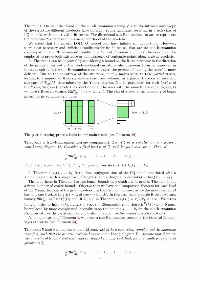
As Theorem 1 can be improved by considering a bound on the Ricci curvature in the directionof the geodesic, instead of the whole sectional curvature, also Theorem 3 can be improved inthe same spirit. In the sub-Riemannian case, however, the process of “taking the trace” is moredelicate. Due to the anisotropy of the structure, it only makes sense to take partial traces,leading to a number of Ricci curvatures (each one obtained as a partial trace on an invariantsubspace of Tγ(t)M , determined by the Young diagram D). In particular, for each level α ofthe Young diagram (namely the collection of all the rows with the same length equal to, say, `)we have ` Ricci curvatures Ricαiγ(t), for i = 1, . . . , `. The size of a level is the number r of boxes

in each of its columns α1, . . . , α`.

α1 α2 α3 α`. . .

size r level α of D

The partial tracing process leads to our main result (see Theorem 29).

Theorem 4 (sub-Riemannian average comparison). Let γ(t) be a sub-Riemannian geodesicwith Young diagram D. Consider a fixed level α of D, with length ` and size r. Then, if

1

rRicαiγ(t) ≥ ki, ∀i = 1, . . . , `, ∀t ≥ 0,

the first conjugate time tc(γ) along the geodesic satisfies tc(γ) ≤ tc(k1, . . . , k`).

In Theorem 4, tc(k1, . . . , k`) is the first conjugate time of the LQ model associated with aYoung diagram with a single row, of length `, and a diagonal potential Q = diagk1, . . . , k`.

The hypotheses in Theorem 4 are no longer bounds on a quadratic form as in Theorem 3, buta finite number of scalar bounds. Observe that we have one comparison theorem for each levelof the Young diagram of the given geodesic. In the Riemannian case, as we discussed earlier, Dhas only one level, of length ` = 1, of size r = dimM . In this case there is single Ricci curvature,namely Ricα1

γ(t) = Ric∇(γ(t)) and, if k1 > 0 in Theorem 4, tc(k1) = π/√k1 < +∞. We stress

that, in order to have tc(k1, . . . , k`) < +∞, the Riemannian condition Ric∇(γ) ≥ k1 > 0 mustbe replaced by more complicated inequalities on the bounds k1, . . . , k` on the sub-RiemannianRicci curvatures. In particular, we allow also for some negative values of such constants.

As an application of Theorem 4, we prove a sub-Riemannian version of the classical Bonnet-Myers theorem (see Theorem 33).

Theorem 5 (sub-Riemannian Bonnet-Myers). Let M be a connected, complete sub-Riemannianmanifold, such that the generic geodesic has the same Young diagram D. Assume that there ex-ists a level α of length ` and size r and constants k1, . . . , k` such that, for any length parametrizedgeodesic γ(t)

1

rRicαiγ(t) ≥ ki, ∀i = 1, . . . , `, ∀t ≥ 0.

4

Then, if the polynomial

Pk1,...,k`(x) := x2` −`−1∑i=0

(−1)`−ik`−ix2i

has at least one simple purely imaginary root, the manifold is compact, has diameter not greaterthan tc(k1, . . . , k`) < +∞. Moreover, its fundamental group is finite.

In the Riemannian setting ` = 1, r = dimM and the condition on the roots of Pk1(x) = x2+k1

is equivalent to k1 > 0. Then we recover the classical Bonnet-Myers theorem (see Theorem 2).Finally we apply our techniques to obtain information about the conjugate time of geodesics

on 3D unimodular Lie groups. Left-invariant structures on 3D Lie groups are the basic examplesof sub-Riemannian manifolds and the study of such structures is the starting point to understandthe general properties of sub-Riemannian geometry.

A complete classification of such structures, up to local sub-Riemannian isometries, is givenin [4, Thm. 1], in terms of the two basic geometric invariants χ ≥ 0 and κ, that are constant forleft-invariant structures. In particular, for each choice of the pair (χ, κ), there exists a uniqueunimodular group in this classification. Even if left-invariant structures possess the symmetriesinherited by the group structure, the sub-Riemannian geodesics and their conjugate loci havebeen studied only in some particular cases where explicit computations are possible.

The conjugate locus of left-invariant structures has been completely determined for the casescorresponding to χ = 0, that are the Heisenberg group [20] and the semisimple Lie groupsSU(2),SL(2) where the metric is defined by the Killing form [18]. On the other hand, whenχ > 0, only few cases have been considered up to now. In particular, to our best knowledge,only the sub-Riemannian structure on the group of motions of the Euclidean (resp. pseudo-Euclidean) plane SE(2) (resp. SH(2)), where χ = κ > 0 (resp. χ = −κ > 0), has beenconsidered [24, 30, 19].

As an application of our results, we give an explicit sufficient condition for a geodesic γ ona unimodular Lie group to have a finite conjugate time, together with an estimate of it. Thecondition is expressed in terms of a lower bound on a constant of the motion E(γ) associatedwith the given geodesic (see Theorem 37).

Theorem 6 (Conjugate points for 3D structures). Let M be a 3D unimodular Lie group endowedwith a contact left-invariant sub-Riemannian structure with invariants χ > 0 and κ ∈ R. Thenthere exists E = E(χ, κ) such that every length parametrized geodesic γ with E(γ) ≥ E has afinite conjugate time.

The cases corresponding to χ = 0 are H, SU(2) and SL(2), where κ = 0, 1,−1, respectively.For these structures we recover the exact estimates for the first conjugate time of a lengthparametrized geodesic (see Section 7.2.1).

1.1. Related literature. The curvature employed in this paper has been introduced for thefirst time by Agrachev and Gamkrelidze in [7], Agrachev and Zelenko in [11] and successivelyextended by Zelenko and Li in [33], where also the Young diagram is introduced for the firsttime in relation with the extremals of a variational problem. This paper is not the first oneto investigate comparison-type results on sub-Riemannian manifolds, but has been inspired bymany recent works in this direction that we briefly review.

In [8] Agrachev and Lee investigate a generalisation of the measure contraction property(MCP) to 3D sub-Riemannian manifolds. The generalised MCP of Agrachev and Lee is ex-pressed in terms of solutions of a particular 2D matrix Riccati equation for sub-Riemannianextremals, and this is one of the technical points that mostly inspired the present paper.

In [22] Lee, Li and Zelenko pursue further progresses for sub-Riemannian Sasakian contactstructures, which posses transversal symmetries. In this case, it is possible to exploit theRiemannian structure induced on the quotient space to write the curvature operator, and theauthors recover sufficient condition for the contact manifold to satisfy the generalised MCPdefined in [8]. Moreover, the authors perform the first step in the decoupling of the matrix

5

Riccati equation for different levels of the Young diagram (see the splitting part of the proof ofTheorem 29 for more details).

The MCP for higher dimensional sub-Riemannian structures has also been investigated in[29] for Carnot groups.

We also mention that, in [23], Li and Zelenko prove comparison results for the number of con-jugate points of curves in a Lagrange Grassmanian associated with sub-Riemannian structureswith symmetries. In particular, [23, Cor. 4] is equivalent to Theorem 3, but obtained with dif-ferential topology techniques and with a different language. However, to our best knowledge, itis not clear how to obtain an averaged version of such comparison results with these techniques,and this is yet another motivation that led to Theorem 4.

In [16], Baudoin and Garofalo prove, with heat-semigroup techniques, a sub-Riemannian ver-sion of the Bonnet-Myers theorem for sub-Riemannian manifolds with transverse symmetriesthat satisfy an appropriate generalisation of the Curvature Dimension (CD) inequalities intro-duced in the same paper. In [17], Baudoin and Wang generalise the previous results to contactsub-Riemannian manifolds, removing the symmetries assumption. See also [15, 14] for othercomparison results following from the generalised CD condition.

Even though in this paper we discuss only sub-Riemannian structures, these techniques can beapplied to the extremals of any affine optimal control problem, a general framework including(sub)-Riemannian, (sub)-Finsler manifolds, as discussed in [6]. For example, in [7], the au-thors prove a comparison theorem for conjugate points along extremals associated with regularHamiltonian systems, such as those corresponding to Riemannian and Finsler geodesics. Finally,concerning comparison theorems for Finsler structures one can see, for example, [26, 27, 32].

1.2. Structure of the paper. The plan of the paper is as follows. In Sec. 2 we providethe basic definitions of sub-Riemannian geometry, and in particular the growth vector and theYoung diagram of a sub-Riemannian geodesic. In Sec. 3 we revisit the theory of Jacobi fields.In Sec. 4 we introduce the main technical tool, that is the generalised matrix Riccati equation,and the appropriate comparison models. Then, in Sec. 5 we provide the “average” version ofour comparison theorems, transitioning from sectional-curvature type results to Ricci-curvaturetype ones. In Sec. 6, as an application, we prove a sub-Riemannian Bonnet-Myers theorem.Finally, in Sec. 7, we apply our theorems to obtain some new results on conjugate points for 3Dleft-invariant sub-Riemannian structures.

2. Preliminaries

Let us recall some basic facts in sub-Riemannian geometry. We refer to [5] for further details.Let M be a smooth, connected manifold of dimension n ≥ 3. A sub-Riemannian structure on

M is a pair (D , 〈·|·〉) where D is a smooth vector distribution of constant rank k ≤ n satisfyingthe Hormander condition (i.e. LiexD = TxM , ∀x ∈M) and 〈·|·〉 is a smooth Riemannian metricon D . A Lipschitz continuous curve γ : [0, T ]→M is horizontal (or admissible) if γ(t) ∈ Dγ(t)

for a.e. t ∈ [0, T ]. Given a horizontal curve γ : [0, T ]→M , the length of γ is

`(γ) =

∫ T

0‖γ(t)‖dt,

where ‖ · ‖ denotes the norm induced by 〈·|·〉. The sub-Riemannian distance is the function

d(x, y) := inf`(γ) | γ(0) = x, γ(T ) = y, γ horizontal.The connectedness of M and the Hormander condition guarantee the finiteness and the conti-nuity of d : M ×M → R with respect to the topology of M (Rashevsky-Chow theorem). Thespace of vector fields on M (smooth sections of TM) is denoted by Vec(M). Analogously, thespace of horizontal vector fields on M (smooth sections of D) is denoted by VecD(M).

Example 1. A sub-Riemannian manifold of odd dimension is contact if D = kerω, where ωis a one-form and dω|D is non degenerate. The Reeb vector field X0 ∈ Vec(M) is the uniquevector field such that dω(X0, ·) = 0 and ω(X0) = 1.

6

Example 2. Let M be a Lie group, and Lx : M → M be the left translation by x ∈ M . Asub-Riemannian structure (D , 〈·|·〉) is left-invariant if dyLx : Dy → DLxy and is an isometryw.r.t. 〈·|·〉 for all x, y ∈M . Any Lie group admits left invariant structures obtained by choosinga scalar product on its Lie algebra and transporting it on the whole M by left translation.

Locally, the pair (D , 〈·|·〉) can be given by assigning a set of k smooth vector fields that spanD , orthonormal for 〈·|·〉. In this case, the set X1, . . . , Xk is called a local orthonormal framefor the sub-Riemannian structure. Finally, we can write the system in “control form”, namelyfor any horizontal curve γ : [0, T ]→M there is a control u ∈ L∞([0, T ],Rk) such that

γ(t) =k∑i=1

ui(t)Xi|γ(t), a.e. t ∈ [0, T ].

2.1. Minimizers and geodesics. A sub-Riemannian geodesic is an admissible curve γ :[0, T ]→M such that ‖γ(t)‖ is constant and for every sufficiently small interval [t1, t2] ⊆ [0, T ],the restriction γ|[t1,t2] minimizes the length between its endpoints. The length of a geodesic isinvariant by reparametrization of the latter. Geodesics for which ‖γ(t)‖ = 1 are called lengthparametrized (or of unit speed). A sub-Riemannian manifold is said to be complete if (M,d) iscomplete as a metric space.

With any sub-Riemannian structure we associate the Hamiltonian function H ∈ C∞(T ∗M)

H(λ) =1

2

k∑i=1

〈λ,Xi〉2, ∀λ ∈ T ∗M,

in terms of any local frame X1, . . . , Xk, where 〈λ, ·〉 denotes the action of the covector λ onvectors. Let σ be the canonical symplectic form on T ∗M . With the symbol ~a we denote theHamiltonian vector field on T ∗M associated with a function a ∈ C∞(T ∗M). Indeed ~a is definedby the formula da = σ(·,~a). For i = 1, . . . , k let hi ∈ C∞(T ∗M) be the linear-on-fibers functionsdefined by hi(λ) := 〈λ,Xi〉. Notice that

H =1

2

k∑i=1

h2i ,

~H =

k∑i=1

hi~hi.

Trajectories minimizing the distance between two points are solutions of first-order necessaryconditions for optimality, which in the case of sub-Riemannian geometry are given by a weakversion of the Pontryagin Maximum Principle ([28], see also [5] for an elementary proof). Wedenote by π : T ∗M →M the standard bundle projection.

Theorem 7. Let γ : [0, T ] → M be a sub-Riemannian geodesic associated with a non-zerocontrol u ∈ L∞([0, T ],Rk). Then there exists a Lipschitz curve λ : [0, T ] → T ∗M , such thatπ λ = γ and only one of the following conditions holds for a.e. t ∈ [0, T ]:

(i) λ(t) = ~H|λ(t) and hi(λ(t)) = ui(t),

(ii) λ(t) =

k∑i=1

ui(t)~hi|λ(t), λ(t) 6= 0 and hi(λ(t)) = 0.

If λ : [0, T ] → M is a solution of (i) (resp. (ii)) it is called a normal (resp. abnormal)extremal). It is well known that if λ(t) is a normal extremal, then its projection γ(t) := π(λ(t))is a smooth geodesic. This does not hold in general for abnormal extremals. On the other hand,a geodesic can be at the same time normal and abnormal, namely it admits distinct extremals,satisfying (i) and (ii). In the Riemannian setting there are no abnormal extremals.

Definition 8. A geodesic γ : [0, T ] → M is strictly normal if it is not abnormal. It is calledstrongly normal if for every t ∈ (0, T ], the segment γ|[0,t] is not abnormal.

7

Notice that extremals satisfying (i) are simply integral lines of the Hamiltonian field ~H.

Thus, let λ(t) = et~H(λ0) denote the integral line of ~H, with initial condition λ(0) = λ0. The

sub-Riemannian exponential map starting from x0 is

Ex0 : T ∗x0M →M, Ex0(λ0) := π(e~H(λ0)).

Unit speed normal geodesics correspond to initial covectors λ0 ∈ T ∗M such that H(λ) = 1/2.

2.2. Geodesic flag and Young diagram. In this section we introduce a set of invariants of asub-Riemannian geodesic, namely the geodesic flag, and a useful graphical representation of thelatter: the Young diagram. The concept of Young diagram in this setting appeared for the firsttime in [33], as a fundamental invariant for curves in the Lagrange Grassmanian. The proofthat the original definition in [33] is equivalent to the forthcoming one can be found in [6, Sec.6], in the general setting of affine control systems.

Let γ(t) be a normal sub-Riemannian geodesic. By definition γ(t) ∈ Dγ(t) for all times.Consider a smooth horizontal extension of the tangent vector, namely an horizontal vector fieldT ∈ VecD(M) such that T|γ(t) = γ(t).

Definition 9. The flag of the geodesic γ(t) is the sequence of subspaces

F iγ(t) := spanLjT(X)|γ(t) | X ∈ VecD(M), j ≤ i− 1 ⊆ Tγ(t)M, i ≥ 1,

where LT denotes the Lie derivative in the direction of T.

By definition, this is a filtration of Tγ(t)M , i.e. F iγ(t) ⊆ F i+1

γ (t), for all i ≥ 1. Moreover,

F 1γ (t) = Dγ(t). Definition 9 is well posed, namely does not depend on the choice of the horizontal

extension T (see [6, Sec. 3.4]).For each time t, the flag of the geodesic contains information about how new directions can

be obtained by taking the Lie derivative in the direction of the geodesic itself. In this senseit carries information about the germ of the distribution along the given trajectory, and is themicrolocal analogue of the flag of the distribution.

Definition 10. The growth vector of the geodesic γ(t) is the sequence of integer numbers

Gγ(t) := dim F 1γ (t), dim F 2

γ (t), . . ..

Notice that, by definition, dim F 1γ (t) = dim Dγ(t) = k.

Definition 11. Let γ(t) be a normal sub-Riemannian geodesic, with growth vector Gγ(t). Wesay that the geodesic is:

• equiregular if dim F iγ(t) does not depend on t for all i ≥ 1,

• ample if for all t there exists m ≥ 1 such that dim Fmγ (t) = dimTγ(t)M .

We stress that equiregular (resp. ample) geodesics are the microlocal counterpart of equireg-ular (resp. bracket-generating) distributions. Let di := dim F i

γ − dim F i−1γ , for i ≥ 1 be the

increment of dimension of the flag of the geodesic at each step (with the convention k0 := 0).

Lemma 12. For an equiregular, ample geodesic, d1 ≥ d2 ≥ . . . ≥ dm.

Proof. By the equiregularity assumption, the Lie derivative LT defines surjective linear maps

LT : F iγ(t)/F i−1

γ (t)→ F i+1γ (t)/F i

γ(t), ∀t, i ≥ 1,

where we set F 0γ (t) = 0 (see also [6, Sec. 3.4]). The quotients F i

γ/Fi−1γ have constant

dimension di := dim F iγ − dim F i−1

γ . Therefore the sequence d1 ≥ d2 ≥ . . . ≥ dm is non-increasing.

Notice that any ample geodesic is strongly normal, and for real-analytic sub-Riemannianstructures also the converse is true (see [6, Prop. 3.12]). The generic geodesic is ample andequiregular. More precisely, the set of points x ∈ M such that there a exists non-emptyZariski open set Ax ⊆ T ∗xM of initial covectors for which the associated geodesic is ample and

8

equiregular with the same (maximal) growth vector, is open and dense in M . For more details,see [33, Sec. 5] and [6, Sec. 5.2].

Young diagram. For an ample, equiregular geodesic, the sequence of dimension stabilises, namely

dim Fmγ = dim Fm+j

γ = n for j ≥ 0, and we write Gγ = dim F 1γ , . . . ,dim Fm

γ . Thus,we associate with any ample, equiregular geodesic its Young diagram as follows. Recall thatdi = dim F i

γ − dim F i−1γ defines a decreasing sequence by Lemma 12. Then we can build a

tableau D with m columns of length di, for i = 1, . . . ,m, as follows:

. . .

. . ....

...

# boxes = di

Indeed∑m

i=1 di = n = dimM is the total number of boxes in D. Let us discuss some examples.

Example 3. For a Riemannian structure, the flag of any non-trivial geodesic consists in a singlespace F 1

γ (t) = Tγ(t)M . Therefore Gγ(t) = n and all the geodesics are ample and equiregular.Roughly speaking, all the directions have the same (trivial) behaviour w.r.t. the Lie derivative.

Example 4. Consider a contact, sub-Riemannian manifold with dimM = 2n+ 1, and a non-trivial geodesic γ with tangent field T ∈ VecD(M). Let X1, . . . , X2n be a local frame in aneighbourhood of the geodesic and X0 the Reeb vector field. Let ω be the contact form. Wedefine the invertible bundle map J : D → D by 〈X|JY 〉 = dω(X,Y ), for X,Y ∈ VecD(M).Finally, we split D = JT⊕ JT⊥ along the geodesic γ(t). We obtain

LT(Y ) = 〈JT|Y 〉X0 mod VecD(M), ∀Y ∈ VecD(M).

Therefore, the Lie derivative of fields in JT⊥ does not generate “new directions”. On the otherhand, LT(JT) = X0 up to elements in VecD(M). In this sense, the subspaces JT and JT⊥ aredifferent w.r.t. Lie derivative: the former generates new directions, the latter does not. In theYoung diagram, the subspace JT⊥ corresponds to the rectangular sub-diagram D2, while thesubspace JT⊕X0 corresponds to the rectangular sub-diagram D1 in Fig. 1.b.

D1

D2

(b) (c)(a)

Figure 1. Young diagrams for (a) Riemannian, (b) contact, (c) a more general structure.

See Fig. 1 for some examples of Young diagrams. The number of boxes in the i-th row (i.e.di) is the number of new independent directions in Tγ(t)M obtained by taking (i − 1)-th Liederivatives in the direction of T.

3. Jacobi fields revisited: conjugate points and Riccati equation

Let λ ∈ T ∗M be the covector associated with a strongly normal geodesic, projection of the

extremal λ(t) = et~H(λ). For any ξ ∈ Tλ(T ∗M) we define the field along the extremal λ(t) as

X(t) := et~H∗ ξ ∈ Tλ(t)(T

∗M).

The set of vector fields obtained in this way is a 2n-dimensional vector space, that we callthe space of Jacobi fields along the extremal. In the Riemannian case, the projection π∗ is anisomorphisms between the space of Jacobi fields along the extremal and the classical spaceof Jacobi fields along the geodesic γ. Thus, this definition is equivalent to the standard one

9

in Riemannian geometry, does not need curvature or connection, and works for any stronglynormal sub-Riemannian geodesic.

In Riemannian geometry, the study of one half of such a vector space, namely the subspaceof classical Jacobi fields vanishing at zero, carries information about conjugate points along thegiven geodesic. By the aforementioned isomorphism, this corresponds to the subspace of Jacobifields along the extremal such that π∗X(0) = 0. This motivates the following construction.

For any λ ∈ T ∗M , let Vλ := kerπ∗|λ ⊂ Tλ(T ∗M) be the vertical subspace. We define thefamily of Lagrangian subspaces along the extremal

L(t) := et~H∗ Vλ ⊂ Tλ(t)(T

∗M).

Definition 13. A time t > 0 is a conjugate time for γ if L(t) ∩ Vλ(t) 6= 0. Equivalently, wesay that γ(t) = π(λ(t)) is a conjugate point w.r.t. γ(0) along γ(t). The first conjugate time isthe smallest conjugate time, namely tc(γ) = inft > 0 | L(t) ∩ Vλ(t) 6= 0.

Since the geodesic is strongly normal, the first conjugate time is separated from zero, namelythere exists ε > 0 such that L(t) ∩ Vλ(t) = 0 for all t ∈ (0, ε). Notice that conjugate pointscorrespond to the critical values of the sub-Riemannian exponential map with base in γ(0).In other words, if γ(t) is conjugate with γ(0) along γ, there exists a one-parameter familyof geodesics starting at γ(0) and ending at γ(t) at first order. Indeed, let ξ ∈ Vλ such that

π∗ et~H∗ ξ = 0, then the vector field τ 7→ π∗ eτ

~H∗ ξ is a classical Jacobi field along γ which

vanishes at the endpoints, and this is precisely the vector field of the aforementioned variation.In Riemannian geometry geodesics stop to be minimizing after the first conjugate time. This

remains true for strongly normal sub-Riemannian geodesics (see, for instance, [5]).

3.1. Riemannian interlude. In this section, we recall the concept of parallely transportedframe along a geodesic in Riemannian geometry, and we give an equivalent characterisation interms of a Darboux moving frame along the corresponding extremal lift. Let (M, 〈·|·〉) be aRiemannian manifold, endowed with the Levi-Civita connection ∇ : Vec(M) → Vec(M). Interms of a local orthonormal frame

∇XjXi =

n∑k=1

ΓkijXk, Γkij =1

2

(ckij + cjki + cikj

),

where Γkij ∈ C∞(M) are the Christoffel symbols written in terms of the orthonormal frame.

Notice that Γkij = −Γjik.

Let γ(t) be a geodesic and λ(t) be the associated (normal) extremal, such that λ(t) = ~H|λ(t)

and γ(t) = π λ(t). Let X1, . . . , Xn a parallely transported frame along the geodesic γ(t),i.e. ∇γXi = 0. Let hi : T ∗M → R be the linear-on-fibers functions associated with Xi, definedby hi(λ) := 〈λ,Xi〉. We define the (vertical) fields ∂hi ∈ Vec(T ∗M) such that ∂hi(π

∗g) = 0,and ∂hi(hj) = δij for any g ∈ C∞(M) and i, j = 1, . . . , n. We define a moving frame along theextremal λ(t) as follows

Ei := ∂hi , Fi := −[ ~H,Ei],

where the frame is understood to be evaluated at λ(t). Notice that we can recover the parallelytransported frame by projection, namely π∗Fi|λ(t) = Xi|γ(t) for all i. In the following, for anyvector field Z along an extremal λ(t) we employ the shorthand

Z|λ(t) :=d

dε

∣∣∣∣ε=0

e−ε~H

∗ Z|λ(t+ε) = [ ~H,Z]|λ(t)

to denote the vector field along λ(t) obtained by taking the Lie derivative in the direction of~H of any smooth extension of Z. Notice that this is well defined, namely its value at λ(t) doesnot depend on the choice of the extension. We state the properties of the moving frame in thefollowing proposition.

Proposition 14. The smooth moving frame Ei, Fini=1 has the following properties:10

(i) spanEi|λ(t) = Vλ(t).(ii) It is a Darboux basis, namely

σ(Ei, Ej) = σ(Fi, Fj) = σ(Ei, Fj)− δij = 0, i, j = 1, . . . , n.

(iii) The frame satisfies structural equations

Ei = −Fi, Fi =n∑j=1

Rij(t)Ej ,

for some smooth family of n× n symmetric matrices R(t).

Properties (i)-(iii) uniquely define the moving frame up to orthogonal transformations. More

precisely if Ei, Fjni=1 is another smooth moving frame along λ(t) satisfying (i)-(iii), with some

matrix R(t) then there exist a constant, orthogonal matrix O such that

(1) Ei|λ(t) =n∑j=1

OijEj |λ(t), Fi|λ(t) =n∑j=1

OijFj |λ(t), R(t) = OR(t)O∗.

A few remarks are in order. Property (ii) implies that spanE1, . . . , En, spanF1, . . . , Fn,evaluated at λ(t), are Lagrangian subspaces of Tλ(t)(T

∗M). Eq. (1) reflects the fact that aparallely transported frame is defined up to constant orthogonal transformations. In particular,one could use properties (i)-(iii) to define the parallel transport along γ(t) by Xi|γ(t) := π∗Fi|λ(t).Finally, the symmetric matrix R(t) induces a well defined quadratic form Rγ(t) : Tγ(t)M → R

Rγ(t)(v) :=n∑

i,j=1

Rij(t)vivj , v =n∑i=1

viXi|γ(t) ∈ Tγ(t)M.

Indeed Proposition 14 implies that the definition of Rγ(t) does not depend on the choice of theparallely transported frame.

Lemma 15. Let R∇ : Vec(M)×Vec(M)×Vec(M)→ Vec(M) the Riemannian curvature tensorw.r.t. the Levi-Civita connection. Then

Rγ(v) = 〈R∇(v, γ)γ|v〉, v ∈ TγM,

where we suppressed the explicit dependence on time.

In other words, for any unit vector v ∈ TγM , Rγ(v) = Sec(v, γ) is the sectional curvature ofthe plane generated by v and γ, i.e. the directional curvature in the direction of the geodesic.The proof of Proposition 14 and Lemma 15 can be found in Appendix C.

3.2. Canonical frame. The concept of Levi-Civita connection and covariant derivative is notavailable for general sub-Riemannian structures, and it is not clear how to parallely transport aframe along a sub-Riemannian geodesic. Nevertheless, in [33], the authors introduce a parallelytransported frame along the corresponding extremal λ(t) which, in the spirit of Proposition 14,generalises the concept of parallel transport also to (sufficiently regular) sub-Riemannian ex-tremals.

Consider an ample, equiregular geodesic, with Young diagram D, with k rows, of lengthn1, . . . , nk. Indeed n1 + . . . + nk = n. The moving frame we are going to introduce is indexedby the boxes of the Young diagram, so we fix some terminology first. Each box is labelled “ai”,where a = 1, . . . , k is the row index, and i = 1, . . . , na is the progressive box number, startingfrom the left, in the specified row. Briefly, the notation ai ∈ D denotes the generic box of thediagram. We employ letters from the beginning of the alphabet a, b, c, . . . for rows, and lettersfrom the middle of the alphabet i, j, h, . . . for the position of the box in the row.

We collect the rows with the same length in D, and we call them levels of the Young diagram.In particular, a level is the union of r rows D1, . . . , Dr, and r is called the size of the level. Theset of all the boxes ai ∈ D that belong to the same column and the same level of D is calledsuperbox. We use greek letters α, β, . . . to denote superboxes. Notice that that two boxes ai, bj

11

level 1

level 1

level 2

level 1

level 2

level 3

(b) (c)(a)

Figure 2. Levels (shaded regions) and superboxes (delimited by bold lines) forthe Young diagram of (a) Riemannian, (b) contact, (c) a more general structure.The Young diagram for any Riemannian geodesic has a single level and a singlesuperbox. The Young diagram of any contact sub-Riemannian geodesic has levelstwo levels containing 2 and 1 superboxes, respectively. The Young diagram (c)has three levels with 4, 2, 1 superboxes, respectively.

are in the same superbox if and only if ai and bj are in the same column of D and in possiblydistinct row but with same length, i.e. if and only if i = j and na = nb. See Fig. 2 for examplesof levels and superboxes for Riemannian, contact and more general structures.

Theorem 16 (See [33]). There exists a smooth moving frame Eai, Faiai∈D along the extremalλ(t) such that

(i) spanEai|λ(t) = Vλ(t).(ii) It is a Darboux basis, namely

σ(Eai, Ebj) = σ(Fai, Fbj) = σ(Eai, Fbj) = δabδij , ai, bj ∈ D.

(iii) The frame satisfies structural equations

(2)

Eai = Ea(i−1) a = 1, . . . , k, i = 2, . . . , na,

Ea1 = −Fa1 a = 1, . . . , k,

Fai =∑

bj∈D Rai,bj(t)Ebj − Fa(i+1) a = 1, . . . , k, i = 1, . . . , na − 1,

Fana =∑

bj∈D Rbj,ana(t)Ebj a = 1, . . . , k,

for some smooth family of n× n symmetric matrices R(t), with components Rai,bj(t) =Rbj,ai(t), indexed by the boxes of the Young diagram D. The matrix R(t) is normal inthe sense of [33].

Properties (i)-(iii) uniquely define the frame up to orthogonal transformation that preserve the

Young diagram. More precisely, if Eai, Faiai∈D is another smooth moving frame along λ(t)

satisfying i)-iii), with some normal matrix R(t), then for any superbox α of size r there existsan orthogonal (constant) r × r matrix Oα such that

Eai =∑bj∈α

Oαai,bjEbj , Fai =∑bj∈α

Oαai,bjFbj , ai ∈ α.

Theorem 16 implies that the following objects are well defined:

• The scalar product 〈·|·〉γ(t), depending on γ(t), such that the fields Xai|γ(t) := π∗Fai|λ(t)

along γ(t) are an orthonormal frame.• A splitting of Tγ(t)M , orthogonal w.r.t. 〈·|·〉γ(t)

Tγ(t)M =⊕α

Sαγ(t), Sαγ(t) := spanXai|γ(t) | ai ∈ α,

where the sum is over the superboxes α of D. Notice that the dimension of Sαγ(t) is equal

to the size r of the level in which the superbox α is contained.• The sub-Riemannian directional curvature, defined as the quadratic form Rγ(t) : Tγ(t)M →R whose representative matrix, in terms of an orthonormal frame Xaiai∈D is Rai,bj(t).

12

• For each superbox α, the sub-Riemannian Ricci curvatures

Ricαγ(t) := tr

(Rγ(t)

∣∣Sαγ(t)

)=∑ai∈α

Rγ(t)(Xai),

which is precisely the partial trace of Rγ(t), identified through the scalar product withan operator on Tγ(t)M , on the subspace Sαγ(t) ⊆ Tγ(t)M .

In this sense, each superbox α in the Young diagram corresponds to a well defined subspaceSαγ(t) of Tγ(t)M . Notice that, for Riemannian structures, the Young diagram is trivial with n rows

of length 1, there is a single superbox, Theorem 16 reduces to Proposition 14, the scalar product〈·|·〉γ(t) reduces to the Riemannian product computed along the geodesic γ(t), the orthogonalsplitting is trivial, the directional curvature Rγ(t) = Sec(γ, ·) is the sectional curvature of the

planes containing γ(t) and there is only one Ricci curvature Ricγ(t) = Ric∇(γ(t)), where Ric∇ :Vec(M)→ R is the classical Ricci curvature.

A compact form for the structural equations. We rewrite system (2) in a compact form. In thesequel it will be convenient to split a frame Eai, Faiai∈D in subframes, relative to the rows ofthe Young diagram. For a = 1, . . . , k, the symbol Ea denotes the na-dimensional row vector

Ea = (Ea1, Ea2, . . . , Eana),

with analogous notation for Fa. Similarly, E denotes the n-dimensional row vector

E = (E1, . . . , Ek),

and similarly for F . Let Γ1 = Γ1(D),Γ2 = Γ2(D) be n × n matrices, depending on the Youngdiagram D, defined as follows: for a, b = 1, . . . , k, i = 1, . . . , na, j = 1, . . . , nb, we set

(Γ1)ai,bj := δabδi,j−1,(3)

(Γ2)ai,bj := δabδi1δj1.(4)

It is convenient to see Γ1 and Γ2 as block diagonal matrices, the a-th block on the diagonal beinga na × na matrix with components δi,j−1 and δi1δj1, respectively (see also Eq. (13)). Noticethat Γ1 is nilpotent and Γ2 is idempotent. Then, we rewrite the system (2) as follows(

E F)

=(E F

)( Γ1 R(t)−Γ2 −Γ∗1

).

By exploiting the structural equations, we write a linear differential equation in R2n that rulesthe evolution of the Jacobi fields along the extremal.

3.3. Linearized Hamiltonian. Let ξ ∈ Tλ(T ∗M) and X(t) := et~H∗ ξ be the associated Ja-

cobi field along the extremal. In terms of any moving frame Eai, Faiai∈D along λ(t), it hascomponents (p(t), x(t)) ∈ R2n, namely

X(t) =∑ai∈D

pai(t)Eai|λ(t) + xai(t)Fai|λ(t).

If we choose the canonical frame, using the structural equations, we obtain that the coordinatesof the Jacobi field satisfy the following system of linear ODEs:

(5)

(px

)=

(−Γ1 −R(t)Γ2 Γ∗1

)(px

).

In this sense, the canonical frame is a tool to write the linearisation of the Hamiltonian flowalong the geodesic in a canonical form. The r.h.s. of Eq. (5) is the “linearised Hamiltonianvector field”, written in its normal form (see also Eq. (10)). The linearised Hamiltonian field is,in general, non-autonomous. Notice also that the canonical form of the linearisation dependson the Young diagram D (through the matrices Γ1 and Γ2) and the curvature matrix R(t).

13

In the Riemannian case, D = for any geodesic, Γ1 = 0, Γ2 = I and we recover the classicalJacobi equation, written in terms of an orthonormal frame along the geodesic

x+R(t)x = 0.

3.4. Riccati equation: blow-up time and conjugate time. Now we study, with a singlematrix equation, the space of Jacobi fields along the extremal associated with an ample, equireg-ular geodesic. We write the generic element of L(t) in terms of the frame along the extremal.

Let Eλ(t), Fλ(t) be row vectors, whose entries are the elements of the frame. The action of et~H∗

is meant entry-wise. Then

L(t) 3 et ~H∗ Eλ(0) = Eλ(t)M(t) + Fλ(t)N(t),

for some smooth families M(t), N(t) of n× n matrices. Notice that

M(0) = I, N(0) = 0, detN(t) 6= 0 for t ∈ (0, ε).

The first t > 0 such that detN(t) = 0 is indeed the first conjugate time. By using once againthe structural equations, we obtain the following system of linear ODEs:

d

dt

(MN

)=

(−Γ1 −R(t)Γ2 Γ∗1

)(MN

).

The solution of the Cauchy problem with the initial datum M(0) = I, N(0) = 0 is defined onthe whole interval on which R(t) is defined. The columns of the 2n × n matrix

(MN

)are the

components of Jacobi fields along the extremal w.r.t. the given frame, and they generate then-dimensional subspace of Jacobi fields X(t) along the extremal λ(t) such that π∗X(0) = 0.

Since, for small t > 0, L(t) ∩ L(0) = 0, we have that

L(t) = spanFλ(t) + Eλ(t)V (t), t > 0,

where V (t) := M(t)N(t)−1 is well defined and smooth for t > 0 until the first conjugate time.Since L(t) is a Lagrangian subspace and the canonical frame is Darboux, V (t) is a symmetricmatrix. Moreover it satisfies the following Riccati equation:

(6) V = −Γ1V − V Γ∗1 −R(t)− V Γ2V.

We characterize V (t) as the solution of a Cauchy problem with limit initial condition.

Lemma 17. The matrix V (t) is the unique solution of the Cauchy problem

(7) V = −Γ1V − V Γ∗1 −R(t)− V Γ2V, limt→0+

V −1 = 0,

in the sense that V (t) is the unique solution such that V (t) is invertible for small t > 0 andlimt→0+ V (t)−1 = 0.

Proof. As we already observed, V (t) satisfies Eq. (6). Moreover V (t) is invertible for t > 0small enough, V (t)−1 = N(t)M(t)−1 and limt→0+ V

−1 = 0. The uniqueness follows from thewell-posedness of the limit Cauchy problem. See Lemma 41 in Appendix A.1.

It is well known that the solutions of Riccati equations are not, in general, defined for allt, but they may blow up at finite time. The next proposition relates the occurrence of suchblow-up time with the first conjugate point along the geodesic.

Proposition 18. Let V (t) the unique solution of (7), defined on its maximal interval I ⊆(0,+∞). Let tc := inft > 0| L(t) ∩ Vλ(t) 6= 0 be the first conjugate point along the geodesic.Then I = (0, tc).

Proof. First, we prove that I ⊇ (0, tc). For any t ∈ (0, tc), L(t) is transversal to Vλ(t). Then the

matrix N(t) is non-degenerate for all t ∈ (0, tc). Then V (t) := M(t)N(t)−1 is the solution of(7), and I ⊇ (0, tc).

14

By contradiction, assume that I ⊃ (0, tc). Consider the n-dimensional smooth families ofsubspaces of Tλ(t)(T

∗M):

L(t) = spanFλ(t)N(t) + Eλ(t)M(t), t ∈ [0,+∞),

L(t) = spanFλ(t) + Eλ(t)V (t), t ∈ I.

Observe that L(t) ∩ Vλ(t) = 0 for all t ∈ I. On (0, tc) we have V (t) = M(t)N(t)−1, hence

L(t) = L(t) on this interval. By continuity, also L(tc) = L(tc). But the first subspace intersectsVλ(tc) (by definition of tc), while the second does not (by construction).

Proposition 18 states that the problem of finding the first conjugate time is equivalent to thestudy of the blow-up time of the Cauchy problem (7) for the Riccati equation.

4. Microlocal comparison theorem

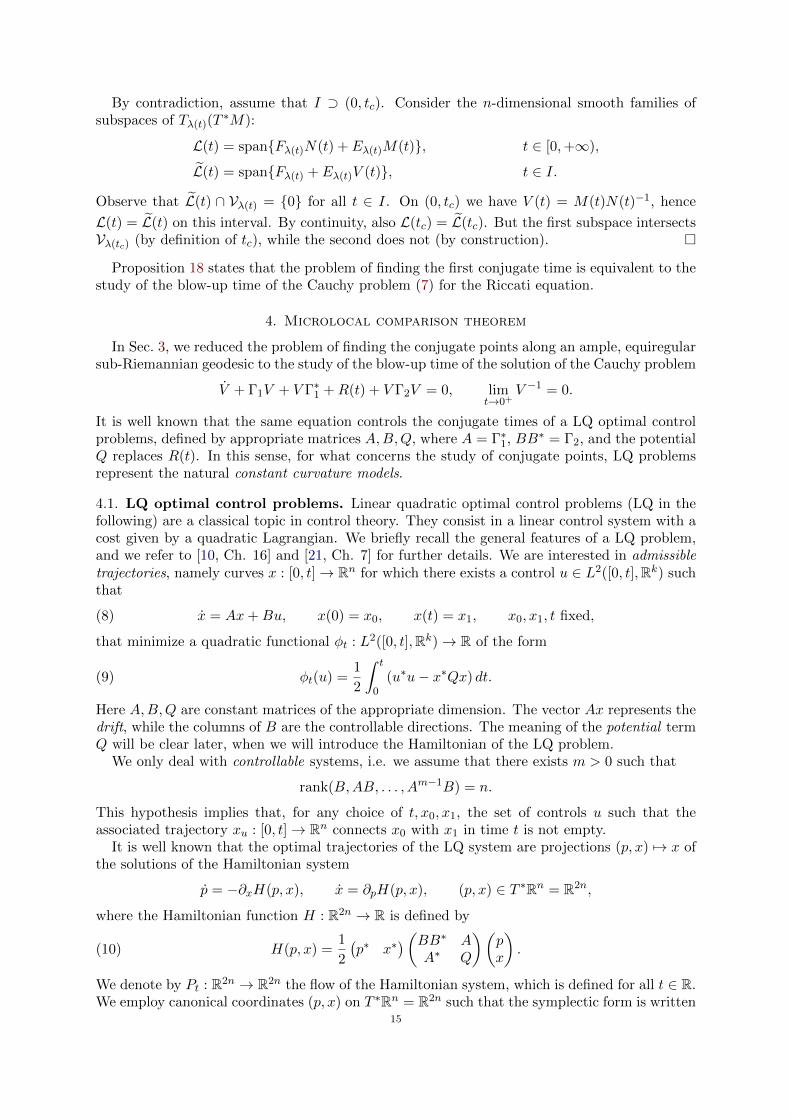
In Sec. 3, we reduced the problem of finding the conjugate points along an ample, equiregularsub-Riemannian geodesic to the study of the blow-up time of the solution of the Cauchy problem

V + Γ1V + V Γ∗1 +R(t) + V Γ2V = 0, limt→0+

V −1 = 0.

It is well known that the same equation controls the conjugate times of a LQ optimal controlproblems, defined by appropriate matrices A,B,Q, where A = Γ∗1, BB∗ = Γ2, and the potentialQ replaces R(t). In this sense, for what concerns the study of conjugate points, LQ problemsrepresent the natural constant curvature models.

4.1. LQ optimal control problems. Linear quadratic optimal control problems (LQ in thefollowing) are a classical topic in control theory. They consist in a linear control system with acost given by a quadratic Lagrangian. We briefly recall the general features of a LQ problem,and we refer to [10, Ch. 16] and [21, Ch. 7] for further details. We are interested in admissibletrajectories, namely curves x : [0, t]→ Rn for which there exists a control u ∈ L2([0, t],Rk) suchthat

(8) x = Ax+Bu, x(0) = x0, x(t) = x1, x0, x1, t fixed,

that minimize a quadratic functional φt : L2([0, t],Rk)→ R of the form

(9) φt(u) =1

2

∫ t

0(u∗u− x∗Qx) dt.

Here A,B,Q are constant matrices of the appropriate dimension. The vector Ax represents thedrift, while the columns of B are the controllable directions. The meaning of the potential termQ will be clear later, when we will introduce the Hamiltonian of the LQ problem.

We only deal with controllable systems, i.e. we assume that there exists m > 0 such that

rank(B,AB, . . . , Am−1B) = n.

This hypothesis implies that, for any choice of t, x0, x1, the set of controls u such that theassociated trajectory xu : [0, t]→ Rn connects x0 with x1 in time t is not empty.

It is well known that the optimal trajectories of the LQ system are projections (p, x) 7→ x ofthe solutions of the Hamiltonian system

p = −∂xH(p, x), x = ∂pH(p, x), (p, x) ∈ T ∗Rn = R2n,

where the Hamiltonian function H : R2n → R is defined by

(10) H(p, x) =1

2

(p∗ x∗

)(BB∗ AA∗ Q

)(px

).

We denote by Pt : R2n → R2n the flow of the Hamiltonian system, which is defined for all t ∈ R.We employ canonical coordinates (p, x) on T ∗Rn = R2n such that the symplectic form is written

15

σ =∑n

i=1 dpi ∧ dxi. The flow lines of Pt are the integral lines of the Hamiltonian vector field~H ∈ Vec(R2n), defined by dH(·) = σ( · , ~H). More explicitly

(11) ~H(p,x) =

(−A∗ −QBB∗ A

)(px

).

We stress that not all the integral lines of the Hamiltonian flow lead to minimizing solutionsof the LQ problem, since they only satisfy first order conditions for optimality. Sufficientlyshort segments, however, are optimal, but they lose optimality at some time t > 0, called thefirst conjugate time.

Definition 19. We say that t is a conjugate time if there exists a solution of the Hamiltonianequations such that x(0) = x(t) = 0.

The first conjugate time determines existence and uniqueness of minimizing solutions of theLQ problem, as specified by the following proposition (see [10, Sec. 16.4]).

Proposition 20. Let tc be the first conjugate time of the LQ problem (8)-(9)

• For t < tc, for any x0, x1 there exists a unique minimizer connecting x0 with x1 in timet.• For t > tc, for any x0, x1 there exists no minimizer connecting x0 with x1 in time t.

The first conjugate time can be also characterised in terms of blow-up time of a matrix Riccatiequation. Consider the vector subspace of solutions of Hamilton equations such that x(0) = 0.A basis of such a space is given by the solutions (pi(t), xi(t)) with initial condition pi(0) := ei,xi(0) = 0, where ei, for i = 1, . . . , n is the standard basis of Rn. Consider the matrices M , N ,whose columns are the vectors pi(t) and xi(t), respectively. They solve the following equation:

d

dt

(MN

)=

(−A∗ −QBB∗ A

)(MN

),

where M(0) = I and N(0) = 0. Under the controllability condition, N(t) is non-singular fort > 0 sufficiently small. By definition, the first conjugate time of the LQ problem is the first t > 0such that N(t) is singular. Thus, consider V (t) := M(t)N(t)−1. The matrix V (t) is symmetricand is the unique solution of the following Cauchy problem with limit initial condition:

V +A∗V + V A+Q+ V BB∗V = 0, limt→0+

V −1 = 0.

Thus we have the following characterization of the first conjugate time of the LQ problem.

Lemma 21. The maximal interval of definition of the unique solution of the Cauchy problem

V +A∗V + V A+Q+ V BB∗V = 0, limt→0+

V −1 = 0,

is I = (0, tc), where tc is the first conjugate time of the associated LQ optimal control problem.

The same characterisation holds also for conjugate points along sub-Riemannian geodesics(see Proposition 18), and in this sense LQ problems provide models for computing conjugatetimes along sub-Riemannian geodesics.

4.2. Constant curvature models. Let D be a Young diagram associated with some ample,equiregular geodesic, and let Γ1 = Γ1(D), Γ2 = Γ2(D) the matrices defined in Sec. 2. Let Q bea symmetric n× n matrix.

Definition 22. We denote by LQ(D;Q) the constant curvature model, associated with a Youngdiagram D and constant curvature equal to Q, defined by the LQ problem with Hamiltonian

H(p, x) =1

2(p∗BB∗p+ 2p∗Ax+ x∗Qx) , A = Γ∗1, BB∗ = Γ2.

We denote by tc(D;Q) ≤ +∞ the first conjugate time of LQ(D;Q).16

Remark 1. Indeed there are many matrices B such that BB∗ = Γ2, namely LQ problems withthe same Hamiltonian, but their first conjugate time is the same. In particular, without loss ofgenerality, one may choose B = BB∗ = Γ2.

In general, it is not trivial to deduce whether tc(D;Q) < +∞ or not, and this will becrucial in our comparison theorems. Nevertheless we have the following result in terms of the

representative matrix of the Hamiltonian vector field ~H given by Eq. (11) (see [9]).

Theorem 23. The following dichotomy holds true for a controllable LQ optimal control system:

• If ~H has at least one odd-dimensional Jordan block corresponding to a pure imaginaryeigenvalue, the number of conjugate times in [0, T ] grows to infinity for T → ±∞.

• If ~H has no odd-dimensional Jordan blocks corresponding to a pure imaginary eigen-value, there are no conjugate times.

Thus, it is sufficient to put the Hamiltonian vector field ~H of LQ(D;Q), given by

~H '(−Γ1 −QΓ2 Γ∗1

),

in its Jordan normal form, to obtain necessary and sufficient condition for the finiteness of thefirst conjugate time.

Example 5. If D is the Young diagram associated with a Riemannian geodesic, with a singlecolumn with n = dimM boxes (or, equivalently, one single level with 1 superbox), Γ1 = 0,Γ2 = I, and LQ(D; kI) is given by

H(p, x) =1

2

(|p|2 + k|x|2

),

which is the Hamiltonian of an harmonic oscillator (for k > 0), a free particle (for k = 0) or anharmonic repulsor (for k < 0). Extremal trajectories satisfy x+ kx = 0. Moreover

tc(D; kI) =

π√k, k > 0

+∞ k ≤ 0.

Indeed, for k > 0, all extremal trajectories starting from the origin are periodic, and they returnto the origin at t = π/

√k. On the other hand, for k ≤ 0, all trajectories escape at least linearly

from the origin, and we cannot have conjugate times (small variations of any extremal spread

at least linearly for growing time). In this case, the Hamiltonian vector field ~H of LQ(D; kI)has characteristic polynomial P (λ) = (λ2 + k)n. Therefore Theorem 23 correctly gives that thefirst conjugate time is finite if and only if k > 0.

Example 6. For any Young diagram D, consider the model LQ(D; 0). Indeed in this case all

the eigenvalues of ~H vanish. Thus, by Theorem 23, one has tc(D;Q) = +∞.

In the following, when considering average comparison theorems, we will consider a particularclass of models, that we discuss in the following example.

Example 7. Let D = . . . be a Young diagram with a single row of length `, and Q =diagk1, . . . , k`. We denote these special LQ models simply LQ(k1, . . . , k`).

In the case ` = 2, Theorem 23 says that tc(k1, k2) < +∞ if and only ifk1 > 0,

4k2 > −k21,

or

k1 ≤ 0,

k2 > 0.

In particular, by explicit integration of the Hamiltonian flow, one can compute that, if k1 > 0and k2 = 0, the first conjugate time of LQ(k1, 0) is tc(k1, 0) = 2π/

√k1.

17

4.3. General microlocal comparison theorem. We are now ready to prove the main resulton estimates for conjugate times in terms of the constant curvature models LQ(D;Q).

Theorem 24. Let γ(t) be an ample, equiregular geodesic, with Young diagram D. Let Rγ(t) :Tγ(t)M → R be directional curvature in the direction of the geodesic and tc(γ) the first conjugatetime along γ. Then

(i) if Rγ(t) ≥ Q+ for all t ≥ 0, then tc(γ) ≤ tc(D;Q+),(ii) if Rγ(t) ≤ Q− for all t ≥ 0, then tc(γ) ≥ tc(D;Q−),

where Q± : Rn → R are some constant quadratic forms and we understand the identification ofTγ(t)M ' Rn through any orthonormal basis for the scalar product 〈·|·〉γ(t).

In particular, since tc(D; 0) = +∞ (see Example 6), we have the following corollary.

Corollary 25. Let γ(t) be an ample, equiregular geodesic, with Young diagram D. Let Rγ(t) :Tγ(t)M → R be directional curvature in the direction of the geodesic. Then, if Rγ(t) ≤ 0 for allt ≥ 0, there are no conjugate points along the geodesic.

In other words, the first conjugate times of LQ(D;Q) gives an estimate for the first conjugatetime along geodesics with directional curvature Rγ(t) controlled by Q.

Remark 2. Notice that there is no curvature along the direction of motion, that is Rγ(t)(γ(t)) =0. As it is well known in Riemannian geometry, it is possible to “take out the direction of themotion”, considering the restriction of Rγ(t) to the orthogonal complement of γ(t), with respectto 〈·|·〉γ(t), effectively reducing the dimension by one. To simplify the discussion, we do not gointo such details since there is no variation with respect to the classical Riemannian case.

Remark 3. These microlocal theorems apply very nicely to geodesics in the Heisenberg group.In this example we have both geodesics with Rγ(t) = 0 (the straight lines) and geodesics withRγ(t) > 0 (all the others). The former do not have conjugate times (by Theorem 25), while thelatter do all have a finite conjugate time (by Theorem 24). For more details see Section 7.

Proof of Theorem 24. By Proposition 18, the study of the first conjugate time is reduced to thestudy of the blow-up time of the solutions of the Riccati equation.

We precise the meaning of blow-up time of a quadratic form. Let t 7→ V (t) : Rn → Ra continuous family of quadratic forms. For any w ∈ Rn let t 7→ w∗V (t)w. We say thatt ∈ R ∪ ∞ is a blow-up time for V (t) if there exists w ∈ Rn such that

limt→t

w∗V (t)w →∞.

This is equivalent to ask that one of the entries of the representative matrix of V (t) growsunbounded for t → t. If t is a blow-up time for V (t) and, in addition, for any w such thatlimt→t

w∗V (t)w =∞ we have limt→t

w∗V (t)w = +∞ (resp. −∞), we write

limt→t

V (t) = +∞ (resp−∞).

We compare the solution of the Cauchy problem (7) for the matrix V (t) for our extremal:

(12) V = −(I V

)(R(t) Γ1

Γ∗1 Γ2

)(IV

), lim

t→0+V −1 = 0,

and the analogous solution VD;Q for any normal extremal of the model LQ(D;Q±):

VD;Q± = −(I VD;Q±

)(Q± Γ1

Γ∗1 Γ2

)(I

VD;Q±

), lim

t→0+V −1D;Q±

= 0.

By Lemma 41 in Appendix A.1, both solutions are well defined and positive definite for t > 0sufficiently small. By hypothesis, R(t) ≥ Q+ (resp. R(t) ≤ Q−). Therefore

−(Q+ Γ1

Γ∗1 Γ2

)≥ −

(R(t) Γ1

Γ∗1 Γ2

)resp. −

(R(t) Γ1

Γ∗1 Γ2

)≥ −

(Q− Γ1

Γ∗1 Γ2

).

18

Moreover, by definition, limt→0+ V−1D;Q±

(t) = limt→0+ V−1(t) = 0. Therefore, by Riccati com-

parison (Theorem 40 in Appendix A), we obtain

V (t) ≤ VD;Q+(t), resp. V (t) ≥ VD;Q−(t),

for all t > 0 such that both solutions are defined. We need the following two lemmas.

Lemma 26. For any D and Q, the solution VD;Q is monotone non-increasing.

Proof of Lemma 26. It is a general fact that any solution of the symmetric Riccati differentialequation with constant coefficients is monotone (see [1, Thm. 4.1.8]). In other words, for anysolution X(t) of a Cauchy problem with a Riccati equation with constant coefficients

X +A∗X +XA+B +XQX = 0, X(t0) = X0,

we have that X ≥ 0 (for t ≥ t0, where defined) if and only if X(t0) ≥ 0 (true also with reversedand/or strict inequalities). Thus, in order to complete the proof of the lemma, it only suffices

to compute the sign of VD;Q(ε). This is easily done by exploiting the relationship with the

inverse matrix WD;Q = V −1D;Q. Observe that WD;Q(0) = Γ2 ≥ 0. Then WD;Q(t) is monotone

non-decreasing. In particular WD;Q(ε) ≥ 0. This, together with the fact that WD;Q(ε) > 0 for

ε sufficiently small (see Appendix A.1), implies that VD;Q(ε) ≤ 0, and the lemma is proved.

Lemma 27. If a solution V (t) of the Riccati Cauchy problem (12) blows up at time t, then itblows up at −∞, namely

limt→t

V (t) = −∞.

Proof of Lemma 27. IfR(t) is constant, the statement is an immediate consequence of Lemma 26.Remember that R(t) is defined for all times. Then, let q be the smallest eigenvalue of R(t) onthe interval [0, t]. Indeed R(t) ≥ qI. Then, by Riccati comparison, V (t) ≤ VD;qI(t). Since thelatter is monotone non-increasing by Lemma 26, the statement follows.

Now we conclude. Case (i). In this case R(t) ≥ Q+. By Riccati comparison, V (t) ≤ VD;Q+(t)on the interval (0,mintc(γ), tc(D;Q+)). Assume that tc(γ) > tc(D;Q+). Then

limt→tc(D;Q+)

V (t) ≤ limt→tc(D;Q+)

VD;Q+(t) = −∞,

which is a contradiction, then tc(γ) ≤ tc(D;Q+).Case (ii). In this case R(t) ≤ Q−. By Riccati comparison, V (t) ≥ VD;Q− on the interval

(0,mintc(γ), tc(D;Q−)). Assume that tc(γ) < tc(D;Q−). Then

limt→tc(γ)

VD;Q−(t) ≤ limt→tc(γ)

V (t) = −∞,

and we get a contradiction. Thus tc(γ) ≥ tc(D;Q−).

5. Average microlocal comparison theorem

In this section we prove the average version of Theorem 24. Recall that, with any ample,equiregular geodesic γ(t) we associate its Young diagram D. The latter is partitioned in levels,namely the sets of rows with the same length. Let α1, . . . , α` be the superboxes in some givenlevel, of length `. The size r of the level is the number of rows contained in the level (see Fig. 3).To the superboxes αi we associated the Ricci curvatures Ricαiγ(t) for i = 1, . . . , `. Finally, we

recall the definition anticipated in Example 7.

Definition 28. With the symbol LQ(k1, . . . , k`) we denote the LQ model associated with theYoung diagram D with a single row of length `, and with diagonal potentialQ = diag(k1, . . . , k`).With the symbol tc(k1, . . . , k`) we denote the first conjugate time of LQ(k1, . . . , k`).

19

Da1

Da2

Dar

...

α1 α2 α3 α`. . .

Figure 3. Detail of a single level of D of length ` and size r. It consists of therows Da1 , . . . , Dar , each one of length `. The sets of boxes in each column arethe superboxes α1, . . . , α`.

Theorem 29. Let γ(t) be an ample, equiregular geodesic, with Young diagram D. Let α1, . . . , α`be the superboxes in some fixed level, of length ` and size r. Then, if

1

rRicαiγ(t) ≥ ki, ∀i = 1, . . . , `, ∀t ≥ 0,

the first conjugate time tc(γ) along the geodesic satisfies tc(γ) ≤ tc(k1, . . . , k`).

The hypotheses in Theorem 29 are no longer bounds on a quadratic form, but a finite numberof scalar bounds. Observe that we have one comparison theorem for each level of the Youngdiagram of the given geodesic.

Consider the Young diagram of any geodesic of a Riemannian structure. It consists of a singlelevel of length ` = 1, with one superbox α, of size r = n = dimM and Ricαγ(t) = Ric∇(γ(t)).

This, together with the computation of tc(k) of Example 5, recovers the following well knownresult.

Corollary 30. Let γ(t) be a Riemannian geodesic, such that Ric∇(γ(t)) ≥ nk > 0 for all t ≥ 0.

Then the first conjugate time tc(γ) along the geodesic satisfies tc(γ) ≤ π/√k.

Corollary 30 can be refined by taking out the direction of the motion, effectively reducingthe dimension by 1. A similar reduction can be performed in Theorem 29, in the case of a“Riemannian” level of length 1 and size r, effectively reducing the size of by one. We do not gointo details, since such a reduction can be obtained exactly as in the Riemannian case (see [31,Chapter 14] and also Remark 2).

We recall how the averaging procedure is carried out in Riemannian geometry. In this setting,one considers the average of the diagonal elements of V (t), namely the trace, and employs theCauchy-Schwarz inequality to obtain a scalar Riccati equation for trV (t), where the curvaturematrix is replaced by its trace, namely the Ricci curvature along the geodesic. On the otherhand, in the sub-Riemannian setting, non-trivial terms containing matrices Γ1(D) and Γ2(D)appear in the Riccati equation. These terms, upon tracing, cannot be controlled in terms oftrV (t) alone. The failure of such a procedure in genuine sub-Riemannian manifolds is somehowexpected: different directions have a different “behaviour”, according to the structure of theYoung diagram, and it makes no sense to average over all of them. The best we can do is toaverage among the directions corresponding to the rows of D that have the same length, namelyrows in the same level. The proof of Theorem 29 is based on the following two steps.(i) Splitting: The idea is to split the Cauchy problem

V + Γ1V + V Γ∗1 +R(t) + V Γ2V = 0, limt→0+

V −1 = 0,

in several, lower-dimensional Cauchy problems for particular blocks of V (t). In these equations,only some blocks of R(t) appear. In particular, we obtain one Riccati equation for each row ofthe Young diagram D, of dimension equal to the length of the row. The blow-up of a block ofV (t) imples a blow-up time for V (t). Therefore, the presence of finite blow-up time in any oneof these lower dimensional blocks implies a conjugate time for the original problem.

20

(ii) Tracing: After the splitting step, we sum the Riccati equations corresponding to the rowswith the same length, since all these equations are, in some sense, compatible (they have thesame Γ1,Γ2 matrices). In the Riemannian case, this procedure leads to a single, scalar Riccatiequation. In the sub-Riemannian case, we obtain one Riccati equation for each level of theYoung diagram, of dimension equal to the length ` of the level. In this case the curvaturematrix is replaced by a diagonal matrix, whose diagonal elements are the Ricci curvatures ofthe superboxes α1, . . . , α` in the given level. This leads to a finite number of scalar conditions.

Proof of Theorem 29. We split the blocks of the Riccati equation corresponding to the rows ofthe Young diagram D, with k rows D1, . . . , Dk, of length n1, . . . , nk. Recall that the matricesΓ1(D), Γ2(D), defined in Eqs. (3)-(4), are n× n block diagonal matrices

Γi(D) :=

Γi(D1). . .

Γi(Dk)

, i = 1, 2,

the a-th block being the na × na matrices

(13) Γ1(Da) :=

(0 Ina−1

0 0

), Γ2(Da) :=

(1 00 0na−1

),

where Im is the m×m identity matrix and 0m is the m×m zero matrix. Consider the maximalsolution of the Cauchy problem

V + Γ1V + V Γ∗1 +R(t) + V Γ2V = 0, limt→0+

V −1 = 0.

The blow-up of a block of V (t) implies a finite blow-up time for the whole matrix, hence aconjugate time. Thus, consider V (t) as a block matrix. In particular, in the notation of Sec. 3,the block ab, denoted Vab(t) for a, b = 1, . . . , k, is a na × nb matrix with components Vai,bj(t),i = 1, . . . , na, j = 1, . . . , nb. Let us focus on the diagonal blocks

V (t) =

V11(t) ∗. . .

∗ Vkk(t)

.

Consider the equation for the a-th block on the diagonal, which we call Vaa(t), and is a na×namatrices with components Vai,aj(t), i, j = 1, . . . , na. We obtain

Vaa + Γ1Vaa + VaaΓ∗1 + Raa(t) + VaaΓ2Vaa = 0,

where Γi = Γi(Da), for i = 1, 2 are the matrix in Eq. (13), i.e. the a-th diagonal blocks of thematrices Γi(D). Moreover

Raa(t) = Raa(t) +∑b 6=a

Vab(t)Γ2(Db)Vba(t).

The ampleness assumption implies the following limit condition for the block Vaa.

Lemma 31. limt→0+

(Vaa)−1 = 0.

Proof. Without loss of generality, consider the first block V11. We partition the matrix V andW = V −1 in blocks as follows

V =

(V11 V10

V ∗10 V00

),

where the index “0” collects all indices different from 1. By block-wise inversion, W11 =(V −1)11 = (V11 − V10V

−100 V ∗10)−1. By Lemma 41 in Appendix A.1, for small t > 0, V (t) > 0,

hence V00 > 0 as well. Therefore V11 − (W11)−1 = V10V−1

00 V ∗10 ≥ 0. Thus V11 ≥ (W11)−1 > 0and, by positivity, 0 < (V11)−1 ≤ W11 for small t > 0. By taking the limit for t → 0+, sinceW11 → 0, we obtain the statement.

21

We proved that the block Vaa(t) is solution of the Cauchy problem

(14) Vaa + Γ1Vaa + VaaΓ∗1 + Raa(t) + VaaΓ2Vaa = 0, lim

t→0+(Vaa)

−1 = 0.

The crucial observation is the following (see [22] for the original argument in the contact casewith symmetries). Since Γ2(Db) ≥ 0 and Vba = V ∗ab for all a, b = 1, . . . , k, we obtain

(15) Raa(t) = Raa(t) +∑b6=a

Vab(t)Γ2(Db)V∗ab(t) ≥ Raa(t).

We now proceed with the second step of the proof, namely tracing over the level. Consider

Eq. (14) for the diagonal blocks of V (t), with Raa(t) ≥ Raa(t). Now, we average over all the rowsin the same level α. Let ` be the length of the level, namely ` = na, for any row Da1 , . . . , Dar

in the given level (see Fig. 3). Then define the `× ` symmetric matrix:

Vα :=1

r

∑a∈α

Vaa,

where the sum is taken on the indices a ∈ a1, . . . , ar of the rows Da in the given level α. Onceagain, the blow-up of Vα(t) implies also a blow-up for V (t). A computation shows that Vα isthe solution of the following Cauchy problem

Vα + Γ1Vα + VαΓ∗1 +Rα(t) + VαΓ2Vα = 0, limt→0+

Vα = 0,

where Γ2 = Γ2(Da) for any a ∈ α, and the `× ` matrix Rα(t) is defined by

Rα(t) :=1

r

∑a∈α

Raa(t) +1

r

∑a∈α

VaaΓ2Vaa − VαΓ2Vα

=1

r

∑a∈α

Raa(t) +1

r

[∑a∈α

(VaaΓ2)(VaaΓ2)∗ − 1

r

(∑a∈α

VaaΓ2

)(∑a∈α

VaaΓ2

)∗].

The key observation is that the term in square brackets is non-negative, as a consequence ofthe following lemma, whose proof is in Appendix B.

Lemma 32. Let Xara=1, Yara=1 be two sets of `× ` matrices. Then

(16)

(r∑

a=1

X∗aYa

)(r∑b=1

X∗b Yb

)∗≤

∥∥∥∥∥r∑

a=1

Y ∗a Ya

∥∥∥∥∥r∑b=1

X∗bXb.

Here ‖·‖ denotes the operator norm.

Remark 4. Lemma 32 is a generalisation of the Cauchy-Schwarz inequality, in which the scalarproduct in Rr is replaced by a non-commutative product : Mat(`)r×Mat(`)r → Mat(`), suchthat, if X = Xara=1, Y = Yara=1, the product X Y :=

∑ra=1X

∗aYa. Eq. (16) becomes

(X Y )(X Y )∗ ≤ ‖Y Y ‖X X.Then the l.h.s. of Eq. 16 is just the “square of the scalar product”. For ` = 1, we recover theclassical Cauchy-Schwarz inequality.

We apply Lemma 32 to Xa = Γ2Vaa and Ya = Γ2, for a ∈ α = a1, . . . , ar. We obtain∑a∈α

(VaaΓ2)(VaaΓ2)∗ − 1

r

(∑a∈α

VaaΓ2

)(∑a∈α

VaaΓ2

)∗≥ 0,

which implies, together with Eq. (15)

(17) Rα(t) ≥ 1

r

∑a∈α

Raa(t) ≥1

r

∑a∈α

Raa(t).

Notice that, the ij-th component of the sum in the r.h.s. of Eq. (17) is precisely 1r

∑a∈αRai,aj(t),

where i, j = 1, . . . , `. Thus, for any two fixed indices i, j we are considering, in coordinates,22

the trace of the restriction Rγ(t) : Sαiγ(t) → Sαjγ(t), written in terms of any orthonormal basis for

(Tγ(t)M, 〈·|·〉γ(t)). The matrix R(t) is normal (see Theorem 16). Thus, according to [33], such atrace is always zero, unless i = j. Thus only the diagonal elements are non-vanishing and

1

r

∑a∈α

Raa(t) =1

r

Ricα1

γ(t) 0

. . .

0 Ricα`γ(t)

.

Thus, for any level α, the average over the level Vα satisfies the `× ` matrix Riccati equation

Vα + Γ1Vα + VαΓ∗1 +Rα(t) + VαΓ2Vα = 0, limt→0+

V −1α = 0,

and, under our hypotheses, Rα(t) ≥ diagk1, . . . , k`. Therefore, we proceed as in the proof ofTheorem 24, with diagk1, . . . , k` in place of Q+, and we obtain the statement.

6. A sub-Riemannian Bonnet-Myers theorem

As an application of Theorem 29, we prove a sub-Riemannian analogue of the Bonnet-Myerstheorem (see Theorem 2 for the classical statement).

In order to globalize the previous results, we need to consider that different geodesics, evenstarting at the same point, may have different growth vectors. It turns out that the componentsof the growth vector are computed as ranks of matrices whose entries are polynomial functionsof the covector λ(t) associated with the given geodesic γ(t). This is a direct consequenceof Definition 9 and the fact that the sub-Riemannian Hamiltonian is fiber-wise polynomial(actually, quadratic). It follows that, for any x ∈ M , the growth vector Gγ(0), seen as afunction of the initial covector, is constant on an open Zariski subset Ax ⊆ T ∗xM , where itattains its (member-wise) maximal value, given by the maximal growth vector

Gx := k1(x), . . . , km(x), ki(x) := maxλ∈T ∗

xMdim F i

γ(0).

Any sub-Riemannian structure has ample geodesics starting from any given point, thus Ax isnot-empty for every x ∈M (see [6, Sec. 5.2] for a proof). Moreover, all the functions x 7→ ki(x)are bounded, lower semi-continuous with integer values. Thus, the set Ω ⊆ M of points suchthat Gx is locally constant is open and dense.

As a consequence, the generic normal geodesic starting at x ∈ Ω (“generic” means with initialcovector in Ax) is ample and equiregular, at least when restricted to a sufficient short segment.We call Dx the Young diagram of the generic normal geodesic starting at x. The Young diagramDx is “locally constant”, in the sense that for any x ∈ Ω there exists an open set U ⊆ Ω suchthat for all y ∈ U we have Dy = Dx.

The structure of Ω may be complicated, and a geodesics starting from x ∈ Ω may crossregions where Dx has different shapes. To avoid such pathological situations, we make thefollowing assumption:

(?) Ω = M and the Young diagram Dx is constant.

This is equivalent to the existence of a fixed Young diagram D such that, for all x ∈ M , thegeneric normal geodesic (i.e. with initial covector in Ax ⊆ T ∗xM) is ample, equiregular, withthe same Young diagram D. This assumption is satisfied, for instance, by any slow-growthdistribution, a large class of sub-Riemannian structures including any contact, quasi-contact,fat, Engel, Goursat-Darboux distributions (see [6, Sec. 5.5]). Moreover, this assumption issatisfied by all left-invariant structures on Lie groups and, more generally, sub-Riemannianhomogeneous spaces.

Under the assumption (?), with a generic geodesic γ(t) we can associate the directionalcurvature Rγ(t) : Tγ(t)M → R and the corresponding Ricci curvatures Ricαγ(t), one for each

superbox α in D.23

Theorem 33. Let M be a complete, connected sub-Riemannian manifold satisfying (?). Assumethat there exists a level α of length ` and size r of the Young diagram D and constants k1, . . . , k`such that, for any length parametrized geodesic γ(t)

1

rRicαiγ(t) ≥ ki, ∀i = 1, . . . , `, ∀t ≥ 0.

Then, if the polynomial

Pk1,...,k`(x) := x2` −`−1∑i=0

(−1)`−ik`−ix2i

has at least one simple purely imaginary root, the manifold is compact, has diameter not greaterthan tc(k1, . . . , k`) < +∞. Moreover, its fundamental group is finite.

Proof. First, we show that diam(M) := supd(x, y)|x, y ∈ M ≤ tc(k1, . . . , k`). Let x0 ∈ M ,and let Σx0 ⊆ M be the set of points x such that there exists a unique minimizing geodesicconnecting x0 with x, strictly normal and with no conjugate points. We have the followingfundamental result (see [3] or also [6, Thm. 5.8]).

Theorem 34. Let x0 ∈ M . The set Σx0 is open, dense and the sub-Riemannian squareddistance x 7→ d2(x0, x) is smooth on Σx0.

Indeed, the sub-Riemannian exponential map Ex0 : T ∗x0M → M is a smooth diffeomorphism

between Σx0 := E−1x0 (Σx0) ⊆ T ∗x0M and Σx0 . Now consider all the normal geodesics connecting

x0 with points in Σx0 , associated with initial covectors in Σx0 . The generic normal geodesic,with covector in Ax0 ⊆ T ∗x0M is ample and equiregular, with the same growth vector, and thusthe same Young diagram Dx0 = D. Thus, for an open dense set Σ′x0 := Ex0(Ax0) ∩ Σx0 ⊆ M ,there exists a unique geodesic connecting x0 with x ∈ Σ′x0 , and it has Young diagram D.

Now we apply Theorem 29 to all the geodesics connecting x0 with points x ∈ Σ′x0 , and weobtain that the first conjugate time tc along these geodesics satisfies tc ≤ tc(k1, . . . , k`). Thesegeodesics lose optimality after the first conjugate point and, since the geodesics are parametrisedby length, we have that, for any x0 ∈ M , supd(x0, x)|x ∈ Σ′x0 ≤ tc(k1, . . . , k`). By densityof Σ′x0 in M , we obtain that diam(M) ≤ tc(k1, . . . , k`). The condition on the roots of Pk1,...,k`implies that tc(k1, . . . , k`) < +∞, by Theorem 23.

By completeness of M , closed sub-Riemannian balls are compact, hence M is compact. Forthe result about the fundamental group, the argument is the classical one. First, we consider

the universal cover M of M . We define a sub-Riemannian structure on M uniquely by liftingthe sub-Riemannian metric on the evenly covered neighbourhoods. All the local assumptions

of our theorem remain true also on M . The completeness remains true as well. The boundson Ricci curvature still holds since it is only a local concept and the covering map is a local

isometry. Hence we apply Theorem 29 to the covering, and also M is compact. Then any point

q ∈M has a finite number of preimages in M , and so π1(M) is finite since π1(M) is trivial.

Remark 5. In the Riemannian case, Pk1(x) = x2 + k1. Then we recover the classical Bonnet-Myers theorem since, by Example 5, tc(k1) = π/

√k1.

7. Applications to left-invariant structures on 3D unimodular Lie groups

Consider a contact left-invariant sub-Riemannian structure on a 3D manifold. Any non-trivial geodesic is ample, equiregular and has the same Young diagram, with two boxes on thefirst row, and one in the second row (see Example 4). The subspace associated with the boxin the second row corresponds to the direction of the motion, i.e., the tangent vector to thegeodesic. Since the curvature always vanishes in this direction (see Remark 2), we can restrictto a single-level Young diagram α of length ` = 2 and size r = 1. We denote by α1, α2 thetwo boxes of this level. The comparison LQ model is the one discussed in Example 7. Then,Theorem 29 rewrites as follows.

24

Theorem 35. Let γ(t) be a length parametrized geodesic of a contact left-invariant sub-Rie-mannian structure on a 3D manifold. Assume that

Ricαiγ(t) ≥ ki, i = 1, 2, ∀t ≥ 0,

for some k1, k2 such that

(18)

k1 > 0,

4k2 > −k21,

or

k1 ≤ 0,

k2 > 0.

Then tc(γ) ≤ tc(k1, k2) < +∞. If the hypotheses are satisfied for every length parametrisedgeodesic, then the manifold is compact, with diameter not greater than tc(k1, k2). Moreover, itsfundamental group is finite.

In the statement of Theorem 35 we allow also for negative Ricci curvatures. Indeed, ingeneral, Ricα2

γ(t) is not sign-definite along the geodesic.

7.1. Invariants of a 3D contact structure. For invariant of a sub-Riemannian structurewe mean any scalar function that is preserved by isometries. In this section we introduce theinvariants χ, κ of 3D contact sub-Riemannian structures, not necessarily left-invariant. For left-invariant structures, χ and κ are constant and we write the expression for Ricα1

γ(t) and Ricα2

γ(t) in

terms of these quantities. The presentation follows closely the one contained in [4], where theinterested reader can find more details.

Recall that a three-dimensional sub-Riemannian structure is contact if D = kerω, wheredω|Dx is non degenerate, for every x ∈ M . In what follows we normalize the contact structureby requiring that dω|Dx agrees with the volume induced by the inner product on D . TheReeb vector field associated with the contact structure is the unique vector field X0 such thatω(X0) = 1 and dω(X0, ·) = 0. Notice that X0 depends only on the sub-Riemannian structure.For every orthonormal frame X1, X2 on the distribution, we have

[X1, X0] = c101X1 + c2

01X2,

[X2, X0] = c102X1 + c2

02X2,

[X2, X1] = c112X1 + c2

12X2 +X0,

(19)

where ckij ∈ C∞(M). The sub-Riemannian Hamiltonian is

H =1

2(h2

1 + h22),

where hi(λ) = 〈λ,Xi(q)〉 are the linear-on-fibers functions on T ∗M associated with the vectorfields Xi, for i = 0, 1, 2. Length parametrized geodesics are projections of solutions of theHamiltonian system associated with H on T ∗M that are contained in the level set H = 1/2.

The Poisson bracket H,h0 is an invariant of the sub-Riemannian structure and, by defini-tion, it vanishes everywhere if and only if the flow of the Reeb vector field etX0 is a one-parameterfamily of sub-Riemannian isometries. A standard computation gives

H,h0 = c101h

21 + (c2

01 + c102)h1h2 + c2

02h22.

For every x ∈M , the restriction of H,h0 to T ∗xM , that we denote by H,h0x, is a quadraticform on the dual of the distribution D∗x , hence it can be interpreted as a symmetric operator onthe distribution Dx itself. In particular its determinant and its trace are well defined. Moreoverone can show that trH,h0x = c1

01 + c202 = 0, for every x ∈M . The first invariant χ is defined

as the positive eigenvalue of this operator, namely

(20) χ(x) :=√−detH,h0x ≥ 0.

The second invariant κ can be defined via the structure constants (19) as follows:

(21) κ(x) := X2(c112)−X1(c2

12)− (c112)2 − (c2

12)2 +c2

01 − c102

2.

25

One can prove that the expression (21) is invariant by rotation of the orthonormal frame.

Remark 6. The quantities χ, κ were first introduced in [2] as differential invariants appearingin the asymptotic expansion of the cut and conjugate locus of the sub-Riemannian exponentialmap near to the base point.

7.2. Left-invariant structures. For left-invariant structures, the functions ckij and the invari-ants χ, κ, are constant on M can be used to classify the left-invariant structures on three-dimensional Lie groups. In particular, when χ = 0, the unique left-invariant structures (up tolocal isometries) are the Heisenberg group H and the Lie groups SU(2) and SL(2), with metricgiven by the Killing form, corresponding to the choice of κ = 0, 1,−1, respectively. When χ > 0,for each choice of (χ, κ) there exists exactly one unimodular Lie group with these values (see[4, Thm. 1]).

7.2.1. Case χ = 0. When χ = 0, the flow of the Reeb vector field is a one-parameter familyof sub-Riemannian isometries. In particular from the computations contained in [8, Thm. 6.2]one gets that the directional curvature Rγ(t) is diagonal with entries Ricα1

γ(t) and Ricα2

γ(t), where

Ricα1

γ(t) = h20(t) + κ(h2

1(t) + h22(t)), Ricα2

γ(t) = 0.

We stress that λ(t) = (h0(t), h1(t), h2(t)) is the solution of the Hamiltonian system associatedwith H and λ = (h1(0), h2(0), h0(0)) is the initial covector associated with the geodesic γ(t).

For any length-parametrized geodesic H(λ(t)) = 1/2, namely h21(t) + h2

2(t) = 1. Moreoverh0(t) = h0 is a constant of the motion. Thus

Ricα1

γ(t) = h20 + κ, Ricα2

γ(t) = 0.

Notice that Ricα1

γ(t) and Ricα2

γ(t) are constant in t and Rγ(t) is diagonal, so for all these cases we

can apply Theorem 24, computing the exact value of the first conjugate time. In particular,this recovers the following well known results obtained in [20, 18].

• H. In this case κ = 0. If h0 = 0 we have Ricα1

γ(t) = Ricα2

γ(t) = 0 and the geodesic has no

conjugate point. If h0 6= 0 then tc = 2π/|h0|.• SU(2). In this case κ = 1. We have Ricα1

γ(t) = h20 + 1, Ricα2

γ(t) = 0 and every geodesic has

conjugate time tc = 2π/√h2

0 + 1.• SL(2). In this case κ = −1. We have Ricα1

γ(t) = h20−1, Ricα2

γ(t) = 0 and we have two cases.

If h0 ≤ 1 then tc = +∞. If h0 > 1 every geodesic has conjugate time tc = 2π/√h2

0 − 1.

Let us mention that, for SU(2), the first condition of (18) holds for any geodesic. Hence, thanksto Theorem 35, we recover its compactness and the exact estimate on its diameter, equal to 2π.

7.2.2. Case χ > 0. In this section we prove our result on 3D unimodular Lie groups with χ > 0.Let us recall that under these assumptions, there exists a special orthonormal frame for the sub-Riemannian structure. In terms of the latter we provide the explicit expression of a constant ofthe motion.

Proposition 36. Let M be a 3D unimodular Lie group, endowed with a contact left-invariantstructure, with χ > 0. Then there exists a left-invariant orthonormal frame X1, X2 on thedistribution such that

H,h0 = 2χh1h2.

Moreover the Lie algebra defined by the frame X0, X1, X2 satisfies

[X1, X0] = (χ+ κ)X2,

[X2, X0] = (χ− κ)X1,

[X2, X1] = X0.

(22)

26

The function E : T ∗M → R, defined by

E =h2

0

2χ+ h2

2,

is a constant of the motion, i.e., H,E = 0. Finally the curvatures Ricα1γ and Ricα2

γ satisfy:

Ricα1γ = h2

0 + 3χ(h21 − h2

2) + κ(h21 + h2

2),(23)

Ricα2γ = 6χ(h2

1 − h22)h2

0 − 2χ(χ+ κ)h41 − 12χ2h2

1h22 − 2χ(χ− κ)h4

2.(24)

In Eqs. (23) and (24) we suppressed the explicit dependence on t.

Proof. From [4, Prop. 13] it follows that there exists a unique (up to a sign) canonical frameX0, X1, X2 such that

[X1, X0] = c201X2,

[X2, X0] = c102X1,

[X2, X1] = c112X1 + c2

12X2 +X0.

In particular, if the Lie group is unimodular, then the left and the right Haar measures coincide.This implies c1

12 = c212 = 0 (cf. proof of [4, Thm. 1]). Then, from (20) and (21), it follows that

χ = (c201 + c1

02)/2, and κ = (c201 − c1

02)/2, which imply (22).Let us show that, if (22) holds, then H,E = 0. Using that H,h0 = 2χh1h2 and H,h2 =

h1, h2h1 = −h0h1 one gets

H,E =1

χH,h0h0 + 2H,h2h2 = 2h1h2h0 − 2h1h2h0 = 0.

Finally, Eqs. (23) and (24) are simply formulae form [8, Thm. 6.2] specified for left-invariantstructures and rewritten in terms of χ, κ in the frame introduced above (notice that the constantsckij appearing here are the opposite of those used in [8]).

Since E is a constant of the motion, for any length parametrized geodesic γ(t) we denoteby E(γ) the (constant) value of E(λ(t)), where λ(t) is the solution of the Hamiltonian systemassociated with H such that γ(t) = π(λ(t)).

Theorem 37. Let M be a 3D unimodular Lie group, endowed with a contact left-invariantstructure, with χ > 0 and κ ∈ R. Then there exists E = E(χ, κ) such that every lengthparametrized geodesic γ with E(γ) ≥ E has a finite conjugate time.

Proof. We prove that the assumptions of Theorem 35 are satisfied for every geodesic when Eis large enough. Since E is a constant of the motion and H = 1/2 we have

(25) h22 = E − h2

0

2χ, h2

1 = 1− E +h2

0

2χ.

Plugging Eq. (25) into Eqs. (23) and (24), Ricα1

γ(t) and Ricα2

γ(t) are rewritten as follows

Ricα1

γ(t) = 4h20 − 3χ(2E − 1) + κ,

Ricα2

γ(t) = 8h40 − [2κ+ 10χ(2E − 1)]h2

0 + [2χκ(2E − 1) + χ2(8E2 − 8E − 2)].(26)

Since h21 +h2

2 = 1 one has |h2| ≤ 1, from (25) one has the following bound for h0 along the curve

(27) 2χ(E − 1) ≤ h20(t) ≤ 2χE.

Then we have easily a lower bound for Ricα1

γ(t)

Ricα1

γ(t) ≥ 8χ(E − 1)− 3χ(2E − 1) + κ

≥ 2χE − 5χ+ κ =: k1

27

Since we want to prove the result for E large enough, we assume that

E ≥ 1

2

(5− κ

χ

),

so that k1 > 0, and the coefficient of h20 in (26) is negative. Then using (27) one estimates

Ricα2

γ(t) ≥ 2χ2(15− 26E)− 2χκ =: k2

In order to show that the first condition of Eq. (18) of Theorem 35 is satisfied we also compute

(28) 4k2 + k21 = 4χ2E2 + a(χ, κ)E + b(χ, κ),

where a and b are the following quadratic functions

a(χ, κ) = 4χκ− 228χ2, b(χ, κ) = 145χ2 − 18χκ+ κ2.

Since the coefficient of E2 in Eq. (28) is positive, there exists E = E(χ, κ), the largest positiveroot of Eq. (28), such that 4k2 + k2

1 > 0 for all E > E, which ends the proof.

Remark 7. The roots of Eq. (28), and in particular E(χ, κ), depend only on the ratio κ/χ.This means that this number is invariant by rescaling of the sub-Riemannian structure. Thiscould seem strange at a first glance but is a consequence of the fact that we consider onlylength parametrized geodesics. We also stress that, in general, the value E(χ, κ) given by thiscomputation is not sharp.

Appendix A. Comparison theorems for the matrix Riccati equation

The general, non-autonomous, symmetric matrix Riccati equation can be written as follows:

X = R(X; t) := M(t)11 +XM(t)12 +M(t)∗12X +XM(t)22X =(I X

)M(t)

(IX

),

where M(t) is a smooth family of 2n× 2n symmetric matrices. We always assume a symmetricinitial datum, then the solution must be symmetric as well on the maximal interval of definition.All the comparison results are based upon the following theorems.

Theorem 38 (Riccati comparison theorem 1). Let M1(t), M2(t) be two smooth families of2n× 2n symmetric matrices. Let Xi(t) be smooth solution of the Riccati equation

Xi = Ri(Xi; t), i = 1, 2,

on a common interval I ⊆ R. Let t0 ∈ I and (i) M1(t) ≥ M2(t) for all t ∈ I, (ii) X1(t0) ≥X2(t0). Then for any t ∈ [t0,+∞) ∩ I, we have X1(t) ≥ X2(t).

Proof. The proof is a simplified version of [1, Thm. 4.1.4]. Let U := X1−X2. Notice that U issymmetric on the interval I where both solutions are defined. A computation shows that

U = θ(t)U + Uθ(t)∗ +(I X1

)(M1 −M2)

(IX1

),

where

θ(t) = M2(t)∗12 +1

2X1(t)M2(t)22 +

1

2X2(t)M2(t)22.

Taking in account that M1(t)−M2(t) ≥ 0, the matrix U satisfies

U ≥ θ(t)U + Uθ(t)∗.

Indeed U(t0) ≥ 0. Then, the statement follows from the next lemma (see [1, Thm. 4.1.2]).

Lemma 39. Let U be a symmetric solution of the Lyapunov differential inequality

U ≥ θ(t)U + Uθ(t)∗, t ∈ I ⊆ R,

where θ(t) is smooth. Then U(t0) ≥ 0 implies U(t) ≥ 0 for all t ∈ I ∩ [t0,+∞). 28

The assumptions of Theorem 38 involve comparison on coefficients of Riccati equations andon initial data. It can be generalised also for limit initial data as follows.

Theorem 40 (Riccati comparison theorem 2). Let M1(t), M2(t) be two smooth families of2n× 2n symmetric matrices. Let Xi(t) be smooth solutions of the Riccati equation

Xi = Ri(Xi; t), i = 1, 2,

on a common interval I ⊆ R. Let t0 ∈ I. Assume that (i) M1(t) ≥ M2(t) for all t ∈ I,(ii) Xi(t) > 0 for t > t0 sufficiently small, (iii) there exist Yi(t0) := limt→t0+X

−1i (t) and (iv)

Y1(t0) ≤ Y2(t0). Then, for any t ∈ (t0,+∞) ∩ I, we have X1(t) ≥ X2(t).

Proof. Let Yi(t) := Xi(t)−1, defined on some interval (t0, ε) ⊆ I. They satisfy

Yi =(I Yi

)Ni(t)

(IYi

), Ni(t) := −

(0 II 0

)Mi(t)

(0 II 0

), i = 1, 2.

Indeed Yi(t) can be prolonged on [t0, ε] for ε sufficiently small by (iii). Moreover N2(t) ≥ N1(t)by (i) and Y2(t0) ≥ Y1(t0) by (iv). The point t0 belongs to the interval of definition of Yithen, by Theorem 38, Y2(ε) ≥ Y1(ε). By (ii), this implies that X1(ε) ≥ X1(ε). Then we canapply again Theorem 38 to X1 and X2, with t0 = ε, and we obtain that X1(t) ≥ X2(t) for allt ∈ [ε,+∞) ∩ I. Since ε can be chosen arbitrarily close to t0, we obtain the statement.

A.1. Well posedness of limit Cauchy problem. The following lemma justifies the savageuse of the Cauchy problem with limit initial condition. Let A,B, be n× n and n× k matrices,respectively, satisfying the controllability condition

spanB,AB, . . . , AmB = Rn,

for some m ≥ 0. Thus, since the column space of B is equal to the column space of BB∗, wehave that, if we put Γ1 := A∗ and Γ2 := BB∗ ≥ 0,

spanΓ2,Γ1Γ2, . . . ,Γm1 Γ2 = Rn.

This condition is indeed satisfied for the matrices Γ1,Γ2 introduced in Sec. 3.

Lemma 41. For any smooth and symmetric R(t), the Cauchy problem with limit initial condi-tion

(29) V = −Γ1V − V Γ∗1 −R(t)− V Γ2V, limt→0+

V −1 = 0,

is well posed, in the sense that there exists a solution of the Riccati equation, invertible for smallt > 0 such that limt→0+ V

−1 = 0. The solution is symmetric and unique on some maximalinterval of definition I ⊆ (0,+∞). In addition, V (t) > 0 for small t > 0.

Proof. We first prove uniqueness. If two solutions V1, V2 exist, their inverses W1 and W2

(defined for t > 0 sufficiently small) can be extended to smooth matrices on [0, ε), by settingW1(0) = W2(0) = 0. Moreover, they both satisfy the following Cauchy problem:

W = Γ∗1W +WΓ1 + Γ2 +WR(t)W, W (0) = 0.

By uniqueness of the standard Cauchy problem, W1(ε) = W2(ε). Therefore also V −11 (ε) =

V −12 (ε), and uniqueness follows. The choice of ε > 0 for setting the Cauchy datum is irrelevant,

since different choices bring to the same solution. Finally, any solution can be extended uniquelyto a maximal solution, defined on some interval I ⊆ (0,+∞). Notice V (t) and V (t)∗ are bothsolution of (29), in particular V (t) = V (t)∗.

Now, we prove the existence. Consider the Cauchy problem

W = Γ∗1W +WΓ1 + Γ2 +WR(t)W, W (0) = 0.

Its solution is well defined for t ∈ [0, ε). We will soon prove that, for t ∈ (0, ε), such a solutionis positive. Thus V (t) := W (t)−1, defined for t ∈ (0, ε), is a solution of the original Cauchyproblem with limit initial datum, by construction.

29

We are left to prove that, for t > 0 small enough, W (t) > 0. Since R(t) is smooth, fort ∈ [0, ε) we can find k such that R(t) ≥ kI. By comparison Theorem 24, we have that oursolution is bounded below by the solution with R(t) = kI. We write W (t) ≥ Wk(t) ≥ 0 fort ∈ [0, ε) (the last inequality follows again from Theorem 24, by considering the trivial solutionof the Cauchy problem obtained by setting Γ2 = 0).

Assume that, for some small t > 0 and x 6= 0, we have W (t)x = 0. This implies Wk(t)x =0. Being a solution of a Riccati equation with constant coefficients, Wk(t) is monotone non-

decreasing (indeed W (0) = Γ2 ≥ 0, and the same holds true for t ∈ [0, ε) by Lemma 26).Therefore Wk(t)x = 0 identically. Therefore all the derivatives, computed at t = 0, vanishidentically. This imples, after careful examination of the higher derivatives, that

Γ2x = Γ2Γ1x = . . .Γ2Γm1 x = . . . = 0,

that leads to x = 0. This contradicts the assumption, hence W (t) > 0 for t sufficiently small.

Appendix B. Proof of Lemma 32

Lemma. Let Xara=1, Yara=1 be sets of `× ` matrices. Then(r∑

a=1

X∗aYa

)(r∑b=1

X∗b Yb

)∗≤

∥∥∥∥∥r∑

a=1

Y ∗a Ya

∥∥∥∥∥r∑b=1

X∗bXb.

Proof. Let v ∈ R`. Then

v∗

(r∑

a=1

X∗aYa

)(r∑b=1

X∗b Yb

)∗v =

∥∥∥∥∥r∑

a=1

Y ∗aXav

∥∥∥∥∥2

.

Notice the change in position of the transpose. Now, let u ∈ R`, such that ‖u‖ = 1, and

u∗

(r∑

a=1

Y ∗aXav

)=

∥∥∥∥∥r∑

a=1

Y ∗aXav

∥∥∥∥∥ .Then, by the Cauchy-Schwarz inequality, we obtain

(30)

∥∥∥∥∥r∑

a=1

Y ∗aXav

∥∥∥∥∥2

=

∣∣∣∣∣r∑

a=1

(Yau)∗(Xav)

∣∣∣∣∣2

≤r∑

a=1

‖Yau‖2r∑

a=1

‖Xav‖2.

Now, observe that

(31)

r∑a=1

‖Yau‖2 = u∗r∑

a=1

Y ∗a Yau ≤

∥∥∥∥∥r∑

a=1

Y ∗a Ya

∥∥∥∥∥ .Then, plugging Eq. (31) in Eq. (30), we obtain∥∥∥∥∥

r∑a=1

Y ∗aXav

∥∥∥∥∥2

≤

∥∥∥∥∥r∑

a=1

Y ∗a Ya

∥∥∥∥∥r∑b=1

‖Xbv‖2,

which implies the statement.

Appendix C. Proof of Proposition 14 and Lemma 15

In order to prove Proposition 14 and Lemma 15 we define a local frame on T ∗M , associatedwith the choice of a local frame X1, . . . , Xn on M . For i = 1, . . . , n let hi : T ∗M → R bethe linear-on-fibres function defined by hi(λ) := 〈λ,Xi〉. The action of derivations on T ∗M iscompletely determined by the action on affine functions, namely functions a ∈ C∞(T ∗M) suchthat a(λ) = 〈λ, Y 〉 + π∗g for some Y ∈ Vec(M), g ∈ C∞(M). Then, we define the coordinate

lift of a field X ∈ Vec(M) as the field X ∈ Vec(T ∗M) such that X(hi) = 0 for i = 1, . . . , n

and X(π∗g) = X(g). This, together with Leibniz rule, characterize the action of X on affine

functions, and then completely define X. Indeed, by definition, π∗X = X. On the other hand,30

we define the (vertical) fields ∂hi such that ∂hi(π∗g) = 0, and ∂hi(hj) = δij . It is easy to check

that ∂hi , Xini=0 is a local frame on T ∗M . We call such a frame the coordinate lifted frame.

Proof of Proposition 14 and Lemma 15. Point (i) is trivial and follows from the definition ofthe coordinate lifted frame ∂hi . In order to prove point (ii), we compute explicitly

~H =

n∑i=1

hiXi +

n∑j,k=1

hickijhk∂hj

=

n∑i=1

hiXi +

n∑j,k=1

hiΓkijhk∂hj

,

where we used the identities ckij = Γkij − Γkji and Γkij = −Γjik. Then, a direct computation gives

(32) Fi = −[ ~H, ∂hi ] = Xi +n∑

j,k=1

hk

(Γkij + Γikj

)∂hj = Xi +

n∑j,k=1

hkΓkij∂hj ,

where we used the fact that, for a parallely transported frame,∑n

k=1 hkΓikj = 0 and we

suppressed the explicit evaluation at λ(t). Now we are ready to prove point (ii). Indeedσλ(t)(∂hi , ∂hj ) = 0, since Vλ is Lagrangian for all λ. Then

σλ(t)(∂hi ,−[ ~H, ∂hj ]) = −〈Xi|π∗[ ~H, ∂hj ]〉 = δij ,

where we used that π∗[H, ∂hj ] = −Xj , and that for any vertical vector ξ ∈ Vλ and η ∈ Tλ(T ∗M),σ(ξ, η) = 〈ξ|π∗η〉, where we identified ξ with an element of Tπ(λ)M through the scalar product.Finally, by using the r.h.s. of Eq. (32), we obtain

σ(Fi, Fj) =n∑k=1

(Γkijhk − Γkjihk − hkckij

)=

n∑k=1

〈hkXk|∇XiXj −∇XjXi − [Xi, Xj ]〉 = 0,

where we suppressed the explicit dependence on t and the last equality is implied by the vanish-ing of the torsion of Levi-Civita connection. For what concerns point (iii), the first structuralequation is the definition of Fi. By taking the derivative of Fi, we obtain

Fi = [ ~H,Fi] =

n∑`,k,j=1

h`hk〈∇Xi∇X`Xk −∇X`∇XiXk −∇[Xi,X`]Xk|Xj〉Ej .

In particular, this implies Lemma 15, since

Rij(t) =

n∑`,j=1

h`hk〈∇Xi∇X`Xk −∇X`∇XiXk −∇[Xi,X`]Xk|Xj〉 = 〈R∇(Xi, γ)γ|Xj〉,

by definition of Riemann tensor, and the fact that γ(t) =∑n

i=1 hi(λ(t))Xi|γ(t). Finally, let Ei, Fjbe any smooth moving frame along λ(t) satisfying (i)-(iii). We can write, in full generality

Ei =n∑j=1

Aij(t)Ej +Bij(t)Fj , Fi =n∑j=1

Cij(t)Ej +Dij(t)Fj ,

for some smooth families of n×n matrices A(t), B(t), C(t), D(t), where the frame is understoodto be evaluated at λ(t). By imposing conditions (i)-(iii), we obtain that the latter are actuallyconstant, orthogonal matrices, and B = C = 0, thus proving the uniqueness property.

Acknowledgements. The authors are grateful to Andrei Agrachev for fruitful discussions. Theauthors have been supported by Institut Henri Poincare, Paris (RIP program), where most ofthis research has been carried out. The authors have been supported by the European ResearchCouncil, ERC StG 2009 “GeCoMethods”, contract number 239748. The second author hasbeen supported by INdAM (GDRE CONEDP).

31

References

[1] H. Abou-Kandil, G. Freiling, V. Ionescu, and G. Jank. Matrix Riccati Equations: In Control and SystemsTheory. Systems & Control: Foundations & Applications. Springer Verlag NY, 2003.

[2] A. Agrachev. Exponential mappings for contact sub-Riemannian structures. J. Dynam. Control Systems,2(3):321–358, 1996.

[3] A. Agrachev. Any sub-Riemannian metric has points of smoothness. Dokl. Akad. Nauk, 424(3):295–298,2009.

[4] A. Agrachev and D. Barilari. Sub-Riemannian structures on 3D Lie groups. J. Dyn. and Contr. Syst.,18(1):21–44, 2012.

[5] A. Agrachev, D. Barilari, and U. Boscain. Introduction to Riemannian and sub-Riemannian geometry (Lec-ture Notes), http://people.sissa.it/agrachev/agrachev files/notes.html. 2012.

[6] A. Agrachev, D. Barilari, and L. Rizzi. Curvature: a variational approach. Memoirs of the AMS (in press),2013.

[7] A. Agrachev and R. V. Gamkrelidze. Feedback-invariant optimal control theory and differential geometry.I. Regular extremals. J. Dynam. Control Systems, 3(3):343–389, 1997.

[8] A. Agrachev and P. W. Y. Lee. Generalized Ricci curvature bounds for three dimensional contact subrie-mannian manifolds. Math. Ann., 360(1-2):209–253, 2014.

[9] A. Agrachev, L. Rizzi, and P. Silveira. On conjugate times of LQ optimal control problems. Journal ofDynamical and Control Systems, pages 1–17, 2014.

[10] A. Agrachev and Y. L. Sachkov. Control theory from the geometric viewpoint, volume 87 of Encyclopaediaof Mathematical Sciences. Springer-Verlag, Berlin, 2004. Control Theory and Optimization, II.

[11] A. Agrachev and I. Zelenko. Geometry of Jacobi curves. I. J. Dynam. Control Systems, 8(1):93–140, 2002.[12] D. Barilari, U. Boscain, G. Charlot, and R. W. Neel. On the heat diffusion for generic Riemannian and

sub-Riemannian structures. ArXiv e-prints, Oct. 2013.[13] D. Barilari, U. Boscain, and R. W. Neel. Small-time heat kernel asymptotics at the sub-Riemannian cut

locus. J. Differential Geom., 92(3):373–416, 2012.[14] F. Baudoin, M. Bonnefont, and N. Garofalo. A sub-riemannian curvature-dimension inequality, volume

doubling property and the poincar inequality. Mathematische Annalen, pages 1–28, 2013.[15] F. Baudoin, M. Bonnefont, N. Garofalo, and I. H. Munive. Volume and distance comparison theorems for

sub-Riemannian manifolds. J. Funct. Anal., 267(7):2005–2027, 2014.[16] F. Baudoin and N. Garofalo. Curvature-dimension inequalities and Ricci lower bounds for sub-Riemannian

manifolds with transverse symmetries. Journal of the European Mathematical Society (in press), 2014.[17] F. Baudoin and J. Wang. Curvature-dimension inequalities and subelliptic heat kernel gradient bounds on

contact manifolds. Potential Analysis, 40:163, 2014.[18] U. Boscain and F. Rossi. Invariant Carnot-Caratheodory metrics on S3, SO(3), SL(2), and lens spaces.

SIAM J. Control Optim., 47(4):1851–1878, 2008.[19] Y. A. Butt, Y. L. Sachkov, and A. I. Bhatti. Maxwell strata and conjugate points in the sub-riemannian

problem on the lie group SH(2). Journal of Dynamical and Control Systems, pages 1–24, 2016.[20] V. Gershkovich and A. Vershik. Nonholonomic manifolds and nilpotent analysis. J. Geom. Phys., 5(3):407–

452, 1988.[21] V. Jurdjevic. Geometric control theory, volume 52 of Cambridge Studies in Advanced Mathematics. Cam-

bridge University Press, Cambridge, 1997.[22] P. W. Y. Lee, C. Li, and I. Zelenko. Ricci curvature type lower bounds for sub-Riemannian structures on

Sasakian manifolds. Discrete Contin. Dyn. Syst., 36(1):303–321, 2016.[23] C. Li and I. Zelenko. Jacobi equations and comparison theorems for corank 1 sub-Riemannian structures

with symmetries. J. Geom. Phys., 61(4):781–807, 2011.[24] I. Moiseev and Y. L. Sachkov. Maxwell strata in sub-Riemannian problem on the group of motions of a

plane. ESAIM Control Optim. Calc. Var., 16:380–399, 2010.[25] S. B. Myers. Riemannian manifolds with positive mean curvature. Duke Math. J., 8:401–404, 1941.[26] S.-i. Ohta. On the curvature and heat flow on hamiltonian systems. Analysis and Geometry in Metric Spaces,

2, april 2014.[27] S.-i. Ohta and K.-T. Sturm. Bochner–Weitzenbock formula and Li–Yau estimates on Finsler manifolds. Adv.

Math., 252:429–448, 2014.[28] L. S. Pontryagin, V. G. Boltyanskii, R. V. Gamkrelidze, and E. F. Mishchenko. The mathematical theory of

optimal processes. Translated from the Russian by K. N. Trirogoff; edited by L. W. Neustadt. IntersciencePublishers John Wiley & Sons, Inc. New York-London, 1962.

[29] L. Rifford. Ricci curvatures in Carnot groups. Math. Control Relat. Fields, 3(4):467–487, 2013.[30] Y. L. Sachkov. Conjugate and cut time in the sub-Riemannian problem on the group of motions of a plane.

ESAIM Control Optim. Calc. Var., 16:1018–1039, 2010.[31] C. Villani. Optimal transport, volume 338 of Grundlehren der Mathematischen Wissenschaften [Fundamental

Principles of Mathematical Sciences].

32

[32] B. Y. Wu and Y. L. Xin. Comparison theorems in Finsler geometry and their applications. Math. Ann.,337(1):177–196, 2007.

[33] I. Zelenko and C. Li. Differential geometry of curves in Lagrange Grassmannians with given Young diagram.Differential Geom. Appl., 27(6):723–742, 2009.

33