COMPARISON OF TWO PHYSICAL OPTICS ... OF TWO PHYSICAL OPTICS INTEGRATION APPROACHES FOR...

COMPARISON OF TWO PHYSICAL OPTICS

INTEGRATION APPROACHES FOR

ELECTROMAGNETIC SCATTERING

a thesis

submitted to the department of electrical and

electronics engineering

and the institute of engineering and sciences

of bilkent university

in partial fulfillment of the requirements

for the degree of

master of science

By

Ender Ozturk

September, 2008

I certify that I have read this thesis and that in my opinion it is fully adequate,

in scope and in quality, as a thesis for the degree of Master of Science.

Prof. Dr. Ayhan Altıntas (Supervisor)



Prof. Dr. Hayrettin Koymen



Prof. Dr. Birsen Saka

Approved for the Institute of Engineering and Sciences:

Prof. Dr. Mehmet BarayDirector of Institute of Engineering and Sciences

ii

ABSTRACT

COMPARISON OF TWO PHYSICAL OPTICS

INTEGRATION APPROACHES FOR

ELECTROMAGNETIC SCATTERING

Ender Ozturk

M.S. in Electrical and Electronics Engineering

Supervisor: Prof. Dr. Ayhan Altıntas

September, 2008

A computer program which uses two different Physical Optics (PO) approaches

to calculate the Radar Cross Section (RCS) of perfectly conducting planar and

spherical structures is developed. Comparison of these approaches is aimed in

general by means of accuracy and efficiency. Given the certain geometry, it is

first meshed using planar triangles. Then this imaginary surface is illuminated

by a plane wave. After meshing, Physical Optics (PO) surface integral is numer-

ically evaluated over the whole illuminated surface. Surface geometry and ratio

between dimension of a facet and operating wavelength play a significant role in

calculations. Simulations for planar and spherical structures modeled by planar

triangles have been made in order to make a good comparison between the ap-

proaches. Method of Moments (MoM) solution is added in order to establish the

accuracy. Backscattering and bistatic scattering scenarios are considered in sim-

ulations. The effect of polarization of incident wave is also investigated for some

geometry. Main difference between approaches is in calculation of phase differ-

ences. By this study, a comprehensive idea about accuracy and usability due to

computation cost is composed for different PO techniques through simulations

iii

under different circumstances such as different geometries (planar and curved),

different initial polarizations, and different electromagnetic size of facets.

Keywords: Physical Optics (PO), Triangular Surface Meshing, Radar Cross Sec-

tion (RCS), Method of Moments (MoM).

iv

OZET

IKI FIZIKSEL OPTIK INTEGRALI YAKLASIMININ

ELEKTROMANYETIK SACINIM ACISINDAN

KARSILASTIRILMASI

Ender Ozturk

Elektrik ve Elektronik Muhendisligi Bolumu Yuksek Lisans

Tez Yoneticisi: Prof. Dr. Ayhan Altıntas

Eylul, 2008

Iki farklı Fiziksel Optik metodu kullanarak duzlemsel ve kuresel yuzeylerin

Radar Kesit Alanlarını hesaplayan bir bilgisayar programı gelistirilmistir.

Genel itibariyle farklı ilk sartlar icin bu metodların dogruluk ve ver-

imliliginin karsılastırılması amaclanmıstır. Verilen duzlemsel ve kuresel yuzey

oncelikle ucgenleme metodu kullanılarak duzlemlere bolunmustur. Ucgenlemenin

ardından bu duzlemler kullanılarak iki farklı metod ile Fiziksel Optik yuzey

integrali numerik olarak hesaplanmıstır. Kullanılan ucgenlerin elektro-

manyetik buyuklugu ve yuzeyin geometrisi sonuclar uzerinde kayda deger etkiler

olusturmaktadır. Iki metod arasında iyi bir karsılastırma yapabilmek icin pek

cok simulasyon yapılmıstır. Literaturden edinilen Momentler Yontemi sonucu da

gercege en yakın sonucun da degerlendirmesini yapabilmek icin Fiziksel Optik

sonuclarıyla birlikte kullanılmıstır. Gelen dalganın polarizasyonu ile tam iletken

olmayan yuzey ozelliklerinin sacılan dalga uzerine etkisi de kuresel yuzeyler

icin incelenmiıtir. Iki metod arasındaki fark bir ucgen icindeki faz farkının

hesaplanısındadır. Bu calısma ile, iki farklı Fiziksel Optik teknigi arasında

v

farklı yuzey geometrileri (duzlemsel ve kuresel), farklı uyarım polarizasyon-

ları ve farklı elektromanyetik ucgenleme buyukluklukleri icin kapsamlı bir fikir

olusturulmustur.

Anahtar Kelimeler: Fiziksel Optik, yuzey ucgenleme, Radar Kesit Alanı, Mo-

mentler Yontemi.

vi

ACKNOWLEDGMENTS

I would like to thank my supervisor Prof. Ayhan Altıntas for his invaluable

help, encouragement and motivation during my MS studies. I would also like to

thank Dr. Hayrettin Koymen and Dr. Birsen Saka for accepting to be in the

thesis committee and commenting on the thesis. Finally, I would gladly like to

appreciate my beloved wife for her priceless help and belief.

vii

Contents

1 INTRODUCTION 1

2 THEORY 4

2.1 Physical Optics Integral Derivation . . . . . . . . . . . . . . . . . 5

2.2 Triangular Meshing . . . . . . . . . . . . . . . . . . . . . . . . . . 7

2.3 Coordinate Transformation . . . . . . . . . . . . . . . . . . . . . . 12

2.4 Implementation of Approach 1 . . . . . . . . . . . . . . . . . . . . 15

2.5 Implementation of Approach 2 . . . . . . . . . . . . . . . . . . . . 19

3 APPLICATIONS 22

3.1 Applications for Plate Structures . . . . . . . . . . . . . . . . . . 23

3.1.1 Case 1: Observation from Specular Direction . . . . . . . . 23

3.1.2 Case 2: Normal Incidence - Variable Observation . . . . . 26

3.1.3 Case 3: Incidence from a Certain Aspect - Variable Obser-

vation . . . . . . . . . . . . . . . . . . . . . . . . . . . . . 28

3.1.4 Case 4: Incidence from a Certain Aspect - Variable Frequency 29

viii

3.1.5 Case 5: Evaluation of Approaches with Constant Difference 31

3.1.6 Case 6: Applications with Rectangles . . . . . . . . . . . . 33

3.1.7 Case 7: Frequency Applications with Plates . . . . . . . . 37

3.2 Applications with Spherical Structures . . . . . . . . . . . . . . . 38

3.2.1 Case 1: Backscattering Scenario for Spheres . . . . . . . . 39

3.2.2 Case 2: Bistatic Scenario - Different Polarization for Spheres 42

3.2.3 Case 3: Backscattering Scenario for Ellipsoids . . . . . . . 43

3.2.4 Case 4: Special Comparison Regarding the Radius of Cur-

vature in GO Calculation . . . . . . . . . . . . . . . . . . 52

3.2.5 Case 5: Usability Analysis of PO Approaches . . . . . . . 55

3.2.6 Case 6: Time Consumption Analysis of Approaches . . . . 58

4 CONCLUSIONS 59

ix

List of Figures

2.1 Representation of a plate using triangular facets . . . . . . . . . . 8

2.2 Approximation of a sphere using triangular facets . . . . . . . . . 9

2.3 Contouring the target by splitting along the z-axis . . . . . . . . . 10

2.4 Triangular facets on the surface of a sphere . . . . . . . . . . . . . 11

2.5 Local coordinates of a triangle residing in global coordinates . . . 13

2.6 The triangle in local coordinates . . . . . . . . . . . . . . . . . . . 18

3.1 Incident and reflected fields for specular observation . . . . . . . . 24

3.2 Specular observation with 450 facets . . . . . . . . . . . . . . . . 25

3.3 Equal incident and observation angles with 20.000 facets . . . . . 25

3.4 Incident and reflected fields for normal incidence - variable obser-

vation . . . . . . . . . . . . . . . . . . . . . . . . . . . . . . . . . 26

3.5 Scattered power for normal incidence with 8 Facets . . . . . . . . 27

3.6 Scattered power for normal incidence with 2500 facets including

MoM . . . . . . . . . . . . . . . . . . . . . . . . . . . . . . . . . . 28

x

3.7 Incident and reflected fields for incident from a certain aspect-

variable observation . . . . . . . . . . . . . . . . . . . . . . . . . . 29

3.8 Scattered power from π6

incidence with facet number of 512 . . . . 30


incidence with facet number of 32.768 . . 30


incidence with frequency of 3 GHz . . . . 31





3.13 Maximum operation frequency for 3 percent constant difference

between approaches . . . . . . . . . . . . . . . . . . . . . . . . . . 33

3.14 Scattered power for normal incidence from 2m-1m rectangle with

8 facets . . . . . . . . . . . . . . . . . . . . . . . . . . . . . . . . 34

3.15 Scattered power for normal incidence from 2m-1m rectangle with

128 facets . . . . . . . . . . . . . . . . . . . . . . . . . . . . . . . 35

3.16 Scattered power for normal incidence from 1m-1m square plate

with facet size 1/128 m2 . . . . . . . . . . . . . . . . . . . . . . . 35

3.17 Scattered power for normal incidence from 2m-1m rectangular

plate with facet size 1/128 m2 . . . . . . . . . . . . . . . . . . . . 36

3.18 Scattered power for normal incidence from 4m-1m rectangular

plate with facet size 1/128 m2 . . . . . . . . . . . . . . . . . . . . 36

3.19 Scattered power for normal incidence from square plate with 8

facets varying frequency . . . . . . . . . . . . . . . . . . . . . . . 37

3.20 Scattered power for normal incidence from square plate with 512

facets varying frequency . . . . . . . . . . . . . . . . . . . . . . . 38

xi

3.21 Backscattering by φ polarized incident wave with facet number of

10.000 . . . . . . . . . . . . . . . . . . . . . . . . . . . . . . . . . 39


25.600 . . . . . . . . . . . . . . . . . . . . . . . . . . . . . . . . . 40


40.000 . . . . . . . . . . . . . . . . . . . . . . . . . . . . . . . . . 40

3.24 Bistatic scenario for scattering from sphere . . . . . . . . . . . . . 42

3.25 Bistatic scenario: φ polarized incident wave with facet number of

1024 . . . . . . . . . . . . . . . . . . . . . . . . . . . . . . . . . . 44

3.26 Bistatic scenario: θ polarized incident wave with facet number of

1024 . . . . . . . . . . . . . . . . . . . . . . . . . . . . . . . . . . 44


4096 . . . . . . . . . . . . . . . . . . . . . . . . . . . . . . . . . . 45


4096 . . . . . . . . . . . . . . . . . . . . . . . . . . . . . . . . . . 45


16384 . . . . . . . . . . . . . . . . . . . . . . . . . . . . . . . . . . 46


16384 . . . . . . . . . . . . . . . . . . . . . . . . . . . . . . . . . . 46


10.000 at 900MHz . . . . . . . . . . . . . . . . . . . . . . . . . . . 47


10.000 at 900MHz . . . . . . . . . . . . . . . . . . . . . . . . . . . 47

xii


62.500 at 900MHz . . . . . . . . . . . . . . . . . . . . . . . . . . . 48


62.500 at 900MHz . . . . . . . . . . . . . . . . . . . . . . . . . . . 48

3.35 Backscattering scenario for scattering from ellipsoid . . . . . . . . 49

3.36 Backscattering for a oblate spheroid with A=1m and B=0.5m with

facet number 2500 . . . . . . . . . . . . . . . . . . . . . . . . . . 50

3.37 Backscattering for a oblate spheroid with A=1m and B=0.5m with

facet number 10.000 . . . . . . . . . . . . . . . . . . . . . . . . . 50

3.38 Backscattering for a prolate spheroid with A=0.5m and B=1m

with facet number 2500 . . . . . . . . . . . . . . . . . . . . . . . . 51

3.39 Backscattering for a prolate spheroid with A=0.5m and B=1m

with facet number 10.000 . . . . . . . . . . . . . . . . . . . . . . . 51

3.40 Backscattering for a oblate spheroid with A=1m and B=0.5m . . 53

3.41 Backscattering for a sphere with radius R=1/4 . . . . . . . . . . . 53

3.42 Backscattering for a prolate spheroid with A=0.5m and B=1m . . 54

3.43 Backscattering for a sphere with radius R=2 . . . . . . . . . . . . 54

3.44 Backscattering for a sphere with radius R=2 with excess facets . . 55

3.45 Number of facets vs dimension of a facet at the critical frequency 56

3.46 Dimension of facet vs critical frequency . . . . . . . . . . . . . . . 57

3.47 Radius of curvature for constant facet number vs critical frequency 57

3.48 Time consumption of approaches . . . . . . . . . . . . . . . . . . 58

xiii

To my family...

Chapter 1

INTRODUCTION

When a conducting body is illuminated by an electromagnetic wave, electric

currents are induced on the surface of the body. This induction behaves in

accordance with Maxwell’s equations and related electromagnetic boundary con-

ditions. These induced currents act as secondary sources and produce an electro-

magnetic field which is called the scattered field and is a function of the operating

frequency, the polarization of the incident wave and the shape of the scatterer.

The spatial distribution of scattered power density in a certain observation

direction may be expressed by a fictitious cross sectional area called Radar Cross

Section (RCS) which is a function of the shape of the body and the polarization

of incident plane wave. This certain direction is the direction of incident wave in

the backscattering case. RCS is the area through which the flux of the incident

power density would yield the scattered power density isotropically. There are

three RCS regimes that characterize the relationship between the wavelength

and the body size: High Frequency (HF) scattering, resonant scattering and

Low Frequency (LF) scattering.

In the high frequency regime, there are various techniques for calculating

scattered field and/or RCS. Physical Optics (PO) and Geometrical Optics (GO)

1

are the two main ones. GO is based on the classical ray-tracing of incident,

reflected and transmitted rays. PO is based on the integration of induced currents

predicted by GO.

For the GO, RCS is a function of radius of curvature at the specular point,

even in bistatic scattering directions. Specular point may be described as the

intersection point of the shortest path between the incident and observation

point and the scatterer in the existence of reflection. Bistatic scattering means,

separate incident and observation directions. However, this approach may fail

if the surface is flat, since result of the GO blows up for plane wave incidence

because there are infinite number of reflected rays due to the facet that the

radius of curvature is infinite. PO surface integral method, on the other hand,

gives quite fine results around the specular direction [1] even for flat surfaces,

however may fail at wide angles from the specular direction. It is noted that, GO

does not contain diffracted rays and PO diffraction is not accurate. However, as

the frequency is increased, the contribution of diffraction gets smaller. Detailed

information about these techniques may be found in [2] and [3]. Throughout this

thesis, only PO is studied to calculate total scattered field.

In this study, the scattering objects are meshed using triangular plates. This

type of meshing is called triangulation, and each piece of triangles is called a single

facet. Then for each facet, PO scattered field is computed with two different PO

techniques. Adding up field contributions of each facet, total scattered field is

calculated.

For the first approach, introduced in [1], analytical solution of PO radiation

integral for finite flat surfaces is used in calculating field contribution of a single

facet. Since the radiation integral is taken analytically, phase differences within

a facet is taken into account in a precise manner. Induced surface currents are

calculated at each point of a facet and integrated along all points on the mesh.

2

For the second approach, introduced in [4], both induced surface currents and

field produced by this currents are calculated as if there is no phase difference

between any points within a facet. Midpoint of the facet is taken as the reference

point, and, fictitiously, all the area is assumed to be at that point. By this

approximation, instead of taking the integral analytically, a summation of each

mesh contributions is performed for computing total scattered field. Therefore,

a significant amount of computational simplicity is gained in trade-off of the

accuracy of the solution.

A computer program is developed in MATLAB for Radar Cross Section and

scattered field calculations. The calculations are done for some simple shaped

targets as flat plates, PEC spheres and ellipsoids for different polarizations of

initial excitation and various meshing densities. Solutions are compared with

the ones in the literature.

3

Chapter 2

THEORY

Physical Optics is used in this thesis for calculating RCS of targets having con-

ducting surfaces. When a surface is illuminated by a wave, surface currents are

induced. PO calculates the scattered field by integrating this currents over the

whole surface. In order to compute the total field, the surface should be pulled

into pieces. In the implementation, surfaces are represented by small planer tri-

angular facets. Higher the number of facets, better representation of the surface

especially for curved surfaces. Afterwards, scattered field is computed for each

facet and summed up in order to get total field scattered from the body.

In this procedure, there are certain factors which affect the computational cost

and complexity. First of all, computational cost directly depends on the number

of facets. High quality of representation of the body necessitates large number of

facets which boosts up the computation time and allocated memory size during

computation. The results presented here conforms with the PO results in the

literature, [5] and [6].

Two different techniques for evaluation of PO surface integral is introduced

in the following sections:

4

2.1 Physical Optics Integral Derivation

Physical Optics follows the following steps in order to find the scattered field, as

also explained in [7]:

1. Electric and magnetic currents are induced on the illuminated facets and

these currents are found by Geometrical Optics. For Perfect Electric Con-

ductors (PECs), total field is the sum of fields due to incident and reflected

rays.

2. An induced surface current is then a function of the tangential component

of the incident wave. Since GO rays exist only on the illuminated facets,

PO currents for conducting body is given by:

�Js =

⎧⎨⎩

2n × �H i, Illuminated region

0, Shadow region(2.1)

3. Using the radiation integral, the surface current is integrated over the sur-

face.

4. Total field on the surface of a facet is the sum of incident and the reflected

field, which may be expressed with the equations below:

�Et = �Ei + �Es, (2.2)

�H t = �H i + �Hs. (2.3)

Assuming the excitation source is far enough; incident wave is taken as a

plane wave and may be expressed as follows:

�Ei = �Ei0e

−jkki.�r, (2.4)

5

�H i = �H i0e

−jkki.�r. (2.5)

Relation between real and constant amplitude vectors E0 and H0 is given for

plane waves as:

�H i0 =

1

ηki × �Ei

0, (2.6)

where η is the intrinsic impedance of free space, the wavenumber k = w√

εμ and

ki is the unit vector along the propagation vector of incident wave and is given

as:

ki = −(x sin θi cos φi + y sin θi sin φi + z cos θi). (2.7)

The incident electric field is written in terms of its orthogonal components in

spherical coordinates as:

�Ei = ( �Eiθ θ

i + �Eiφφ

i)e−jkki.�r, (2.8)

where (θi, φi) are the spherical coordinates of the source and (ri, θi, φi) are the

unit vectors. The incident magnetic field is given by:

�H i0 =

1

ηki × �Ei

0 (2.9)

=1

η(−Ei

φθi + Ei

θφi)e−jkki.�r. (2.10)

Magnetic vector potential is a useful tool in order to calculate field compo-

nents. This vector potential of the scattered field at �rs is proportional to the

surface integral of induced current and is given by:

6

�As =μ

4πrse−jkrs

∫S

∫�Jejkrs.�rds. (2.11)

Using −jwt time convention, relation between vector potential and electric

field is given as �Es = −jw �As. And applying far field approximation, electric field

expression turns out be:

�Es =jwμ

2πrse−jkrs

∫S

∫n × �H ie−jkks.�rds. (2.12)

Using equations (2.9) and (2.12), the final scattered field is found evaluating

the following equation which is called PO surface integral:

�Es =ejkrs

rs

( �Eiφθ

i − �Eiθφ

i) × (j

λ)

∫S

∫nejk(ri+rs).�rds. (2.13)

2.2 Triangular Meshing

In this study, the target surface is meshed into triangular flat facets, in order to

calculate PO surface integral. To represent these facets, first the whole body is

modeled by enough number of points corresponding to mesh corners. Afterwards,

these points are connected in such a way that Cartesian coordinates of corner

points, midpoint coordinates and the area of each triangle are kept in a main

array of meshing. Meshing process for flat surfaces is explained below:

1. Assuming that, the plate is lying on the x−y plane, two arrays are created

whose elements taking values linearly between [−0.5, 0.5] with sizes equal to

each other depending on how many facets is desired. These arrays represent

the x and y coordinates of corners of triangles.

7

Figure 2.1: Representation of a plate using triangular facets

2. Let the size of the array be N + 1, this means there exists N2 rectangles

on the plate. Therefore, area of a single triangle is constant and found as:

Area = 12N2

3. A third main array is created to hold three coordinates of corners of each

right triangle and midpoint’s coordinates which are derived from corners.

Modeling accuracy is not an issue for flat plates since facets are planar also.

Figure (2.1) is an example for a meshed square plate. However, for curved

surfaces, using flat triangles may cause modeling problems which is inevitable

since infinite number of pieces is needed to perfectly represent a curved surface,

such as a sphere, exactly. On the other hand, increasing the number of facets is

expected to give better results. In this study, only spherical geometries are used

as curved surfaces. In figure (2.2), a meshed sphere is shown. Meshing procedure

for spherical geometries has common points but also different issues:

8

Figure 2.2: Approximation of a sphere using triangular facets

1. The procedure begins with slicing the body into N parallel planes orthog-

onal to the z axis. N should be an even number in order to save the

symmetry and to avoid singularities. (See figure (2.3)) These planes are

expressed as: z = zn(n = 1, 2, ...N) This intervals between slices are deter-

mined due to constant intervals between elevation angles principle.

θn =nπ

N(2.14)

δzn(n) = R(cos(θn) − cos(θn−1)) (2.15)

= R(cos(nπ

N) − cos(

(n − 1)π

N)) (2.16)

= −2R(sin((2n − 1)π

2N) sin(

π

2N)) (2.17)

.

2. Intersection points of a plane and the body is a circle for each plane.

These circles are represented by another array holding x and y coordinates

9

Figure 2.3: Contouring the target by splitting along the z-axis

of points. Therefore with a total number of∑N

n=0

∑M(n)m=0 , (xmn, ymn, zn)

points, the spherical surface is modeled.

3. At the next step, there assumed N pieces of longitudes on the sphere.

Intersection points of these longitudes and horizontally placed circles are

all kept in a main array in order to determine parameters of triangular

facets. In figure (2.4) perpendicular lines are seen. Intermediate regions

between zthn and zth

(n+1) planes and longitudes Lm and Lm+1 are separated

into two triangular pieces. Three points represent a triangle, corners of

the triangle, and all other parameters are derived from these points. Let

PznLm(x, y, z) be a point on the sphere and also the intersection point of zthn

plane and Lthm longitude. Then, three points, PznLm , Pzn+1Lm and PznLm+1

represent the first triangle. Pzn+1Lm, Pzn+1Lm+1 and Pzn+1Lm represent the

second triangle. All three coordinates of all intersection points are known.

10

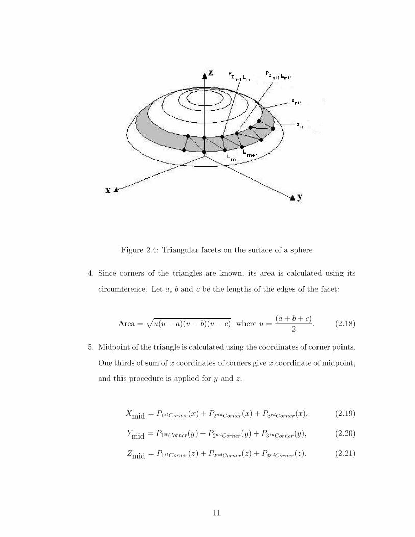
Figure 2.4: Triangular facets on the surface of a sphere

4. Since corners of the triangles are known, its area is calculated using its

circumference. Let a, b and c be the lengths of the edges of the facet:

Area =√

u(u − a)(u − b)(u − c) where u =(a + b + c)

2. (2.18)

5. Midpoint of the triangle is calculated using the coordinates of corner points.

One thirds of sum of x coordinates of corners give x coordinate of midpoint,

and this procedure is applied for y and z.

Xmid = P1stCorner(x) + P2ndCorner(x) + P3rdCorner(x), (2.19)

Ymid = P1stCorner(y) + P2ndCorner(y) + P3rdCorner(y), (2.20)

Zmid = P1stCorner(z) + P2ndCorner(z) + P3rdCorner(z). (2.21)

11

6. Determination of normal vector for each of the facets is an important issue.

It should direct outward to the surface, since all the formulations are de-

rived with this assumption. Regarding a unit sphere centered at the origin

of the coordinate system, it is easy to determine the x, y and z components

of nmn. Under these conditions, coordinates of midpoint, (x, y, z)midpoint,

of a facet is the same as components of normal vector for that facet.

Through these steps, three coordinates of three corners of facets are hold in

addition to the area and coordinates of midpoint of triangles. For planar surfaces,

normal vector is constant and in +z direction for the moment.

2.3 Coordinate Transformation

Before calculating the surface integral, some sort of coordinate transformation is

needed. Each facet is assumed to stand on a local Cartesian coordinate system,

(xl, yl, zl) so that all facets lie on xl−yl plane in calculations. In order to achieve

the transformation, unit vectors for the local coordinates should be defined. Let

�e1, �e2 and �e3 be the edges of the triange in global coordinates. As a starting

point, �e3 may be taken along yl, and one corner of the triangle coincide with the

origin. Then the unit vectors of local system are given by:

yl = − �e3

|�e3| , (2.22)

zl = −�e1 × (−�e3)

|�e1 × �e3| , (2.23)

xl = yl × zl. (2.24)

Local and global coordinate systems are seen on Figure (2.5) for a single facet.

Global coordinates are represented by (xg, yg, zg). In addition, a new parameter

is introduced here, �cl, which is the distance vector between the origins of two

12

Figure 2.5: Local coordinates of a triangle residing in global coordinates

coordinate systems, local and global. Also it is noted that, �rg is the position

vector defined in global coordinates.

First thing to do is to transform incident wave given in rectangular coordi-

nates into local coordinate system. A transform matrix is used for this purpose.

Expression of this matrix m1 is given as:

m1 =

⎛⎜⎜⎜⎝

xg.xl xg.yl xg.zl

yg.xl yg.yl yg.zl

zg.xl zg.yl zg.zl

⎞⎟⎟⎟⎠ . (2.25)

Therefore, initial field in local coordinates may be written in terms of global

coordinates as below:

13

⎛⎜⎜⎜⎝

Eixl

Eiyl

Eiyl

⎞⎟⎟⎟⎠ = m1 ·

⎛⎜⎜⎜⎝

Eixg

Eiyg

Eiyg

⎞⎟⎟⎟⎠ . (2.26)

Second thing is to write the incident field in local spherical coordinate system.

Another transform matrix is used which is called m2 and given as:

m2 =

⎛⎜⎜⎜⎝

xl.θl xl.φl

yl.θl yl.φl

zl.θl zl.φl

⎞⎟⎟⎟⎠ . (2.27)

By applying this transformation, incident field in local spherical coordinate

system is found by

⎛⎝ Ei

θl

Eiφl

⎞⎠ = m2 ·

⎛⎜⎜⎜⎝

Eixl

Eiyl

Eizl

⎞⎟⎟⎟⎠ . (2.28)

The matrix m2 may be written in terms of sines and cosines. This form is

more useful for calculations.

m2 =

⎛⎜⎜⎜⎝

cos θl cos φl − sin φl

cos θl sin φl cos φl

− sin θl 0

⎞⎟⎟⎟⎠ , (2.29)

where θl and φl are azimuth and elevation angles in local coordinates. These

angles may be found from the propagation vector, ki.

Since the matrices m1 and m2 are unitary transformation matrices, transposes

of these matrices may be used for the inverse transformation. Transpose of m1

14

converts local coordinates into global coordinates. Similarly, transpose of m2

converts spherical coordinates into rectangular.

In addition to these, another matrix, mG2 shall be used in the calculations.

This matrix transforms the scattered field from rectangular coordinates into

spherical coordinates in global system:

mG2 =

⎛⎜⎜⎜⎝

xg.θg xg.φg

yg.θg yg.φg

zg.θg zg.φg

⎞⎟⎟⎟⎠ =

⎛⎜⎜⎜⎝

cos θsg cos φs

g − sin φsg

cos θsg sin φs

g cos φsg

− sin θsg 0

⎞⎟⎟⎟⎠ . (2.30)

Mainly there exist two kinds of transformation matrix which are rectangular-

to-spherical and global-to-local transformation matrices. By arranging the pa-

rameters and taking transposes, all the transformation matrices required in cal-

culations may be derived.

2.4 Implementation of Approach 1

The incident electric field in local coordinates is given by

�Eil = (Ei

θlθil + Ei

φlφil)e

j�ki.�rl. (2.31)

Implementation of Physical Optics is described in section 2.1. The θ and φ

components of scattered field as given in equation (2.13) may be written shortly

in local coordinates and in terms of surface currents as:

Esθl(xl, yl) =

−jwμ

4πrejkri

∫S

∫(Jxl cos θ cos φ + Jyl cos θ sin φ − Jzl sin θ)ejkhds′,

(2.32)

15

Esφl(xl, yl) =

−jwμ

4πrejkri

∫S

∫(Jxl sin φ + Jyl cos φ)ejkhds′, (2.33)

where h = x′l sin θ cos φ+ y′

l sin θ sin φ+ z′l cos θ. S in the integral limit stands for

the surface of planar surface of each facet.

Distance from the origin of local coordinate system, �rl may be written in

terms of known parameters. Using far field approximation, �rl turns out to be:

�rl = �rg − (ks.�cl)�cl, (2.34)

where ks is the propagation vector of scattered field and �cl is the distance vector

between origins of global and local coordinate systems pointing local system’s

origin. The equations (2.32) and (2.33) may be written in matrix form:

⎛⎝ Es

θl(r, θ, φ)

Esφl(r, θ, φ)

⎞⎠ =

⎛⎝ Ei

θl

Eiφl

⎞⎠ FI0

jwμ

2πrejkr. (2.35)

The matrix F is the Physical Optics scattering function defined in local co-

ordinates. Its explicit form is as follows:

F =

⎛⎝ − cos θs cos(φs − φi) sin(φs − φi)

− cos θs cos θi sin(φs − φi) − cos θi cos(φs − φi)

⎞⎠ . (2.36)

The difference between two approaches, phase factor, is taken into account

in this approach by the integral I0 which is given by

I0 =

∫ b

x′l=a

∫ β(x′l)

y′l=α(x′

l)

ej(ux′l+vy′

l)dx′dy′, (2.37)

where the unknown terms used in the equation are:

16

u = k(sin θi cos φi + sin θs cos φs), (2.38)

v = k(sin θi sin φi + sin θs sin φs), (2.39)

the terms in the limits of the integral equation are described in figure (2.6) They

may be expressed as:

α(x′l) = α0 + α1x

′l, (2.40)

β(x′l) = β0 + β1x

′l. (2.41)

Considering these equations above, the equation (2.37) may be rewritten as:

I0 =1

jv(ejvβ0

ejb(u+vβ1) − eja(u+jβ1)

j(u + vβ1)− ejvα0

ejb(u+vα1) − eja(u+jα1)

j(u + vα1)). (2.42)

As a result using all the derivations done up to this point, a closed form

expression for the scattered field may be defined:

Es(θg, φg) = Km2(θg, φg) · mT1 · mT

2 (θsl , φ

sl ) · F · m2(θ

il , φ

il) · m1 · �Ei(0). (2.43)

At the left hand side of the equation there exists only one term. Es(θg, φg) is

the far field scattered electric field in global coordinates directed to a spherical

direction represented by the angles θg and φg. On the right hand side, first term

is K, which is a complex constant including phase difference between local and

global coordinate systems:

K = I0jwμ

2πre−jk(r−ki·�cl−ks·�cl). (2.44)

17

Figure 2.6: The triangle in local coordinates

The second term, �Ei(0), is the initial field vector in global coordinates ex-

pressed rectangular system. The next term, m1, converts the incident field into

local rectangular coordinate system. Following term, m2(θil , φ

il) stands for con-

verting rectangular into spherical in local coordinates. The matrix, F , as men-

tioned before, is the Physical Optics scattering matrix. At this point, scattered

field in local spherical coordinates for a single facet is obtained. Then, mT2 (θs

l , φsl )

converts scattered field into Cartesian coordinates in local system. mT1 works for

converting scattered field in local to global coordinate system in Cartesian. Fi-

nally the last term, m2(θg, φg) expresses scattered field in spherical coordinates.

Extending this solution to the whole surface, each scattered field from each

facet should be summed up in order to find total scattered field. Then, the total

field is used to calculate Radar Cross Section of scatterers. Polarization included

expressions for RCS are as follows:

18

σθθ = limr→∞

4πr2 | �Esθ |2

| �Eiθ|2

, (2.45)

σφφ = limr→∞

4πr2| �Es

φ|2| �Ei

φ|2, (2.46)

σθφ = limr→∞

4πr2 | �Esθ |2

| �Eiφ|2

, (2.47)

σφθ = limr→∞

4πr2| �Es

φ|2| �Ei

θ|2. (2.48)

Radar Cross Section (RCS) is a characteristic property of the scattering body

and actually a measure of the power that is returned or scattered in a given

direction, normalized with respect to the power density of the incident field. It

is defined in [8] as the area required to be cut out of the incident wavefront, at

the position of the scatterer, so the power thereby intercepted would, if radiated

isotropically, create the same power density at the observation point as does the

scatterer itself. RCS should be independent from distance of observation point.

This is done by the multiplication factor 4πr2. Including polarization information

of both incident and scattered waves, four possible RCS definitions are given

above. It can be concluded that, RCS is a function of the shape of the target,

operation frequency, incident and observation polarizations.

2.5 Implementation of Approach 2

This approach is easier to implement with respect to previous approach. Imple-

mentation may be continued from the equation (2.13) derived in section 2.1:

�Es =ejkrs

rs(Ei

φθi − Ei

θφi) × (

j

λ)

∫S

∫nejk(ri+rs).�rds. (2.49)

In order to calculate this equation, a new vector quantity should be introduced

here as:

19

�S = (j

λ)

∫ ∫nejk(ri+rs)·�rds, (2.50)

the scattered field may also be written as in its orthogonal components

�Es = (Esθ θs + Es

φφs)e−jkrs

rs. (2.51)

Using (2.13), (2.50), (2.51) and the vector identity given below,

�A · ( �B × �C) = ( �A × �B) · �C, (2.52)

scattered field expressions are found as:

�Esθ = (Ei

θφi × θs + Eiφθs × θi) · �S, (2.53)

�Esφ = (Ei

θφi × φs + Eiφφs × θi) · �S. (2.54)

These two equations can be combined and expressed in matrix form as:

⎛⎝ Es

θ

Esφ

⎞⎠ =

⎛⎝ (φi × θs) · �S (θs × θi) · �S

(φi × φs) · �S (φs × θi) · �S

⎞⎠

⎛⎝ Ei

θ

Eiφ

⎞⎠ . (2.55)

The 2 by 2 matrix in the previous equation is the scattering matrix which

binds the scattered field to incident field component by component. In order

to calculate this matrix, (2.50) should be found first. Since (2.50) is a surface

integral, �S can be calculated by superposing the contributions of each facet. The

difference between this approach and the previous one, contribution of a single

triangle, is written as:

�St = (j

λ)nte

jk(ri+rs)·�rtΔst for t = 1 : C, (2.56)

20

where C is the total number of illuminated facets on the surface of the scatterer

and Δst is the area of tth triangle. Therefore, �S can be expressed as a sum:

�S = (j

λ)

C∑t=0

ntejk(ri+rs)·�rtΔst. (2.57)

Note that only illuminated facets make contribution to the sum in calculating

�S. Therefore, in order to define whether a facet is illuminated or not, a new

parameter is introduced:

It = nt · ri. (2.58)

If It is less then 0, this means that facet is in shadow region. If else, it is

in illuminated region. Simulations and comparisons of these two approaches are

done in the next chapter.

The scattering matrix for the targets which have axial symmetry with respect

to z-axis, closed form expressions for (2.50) can be derived. The results in [9]

well-agrees with the ones calculated in here.

21

Chapter 3

APPLICATIONS

For RCS and scattered power computations, a computer program is written in

MATLAB. The program includes mesh generation code for plate and spherical

geometries. In order to stay in high frequency region, size of the scatterer should

be electrically large, namely large with respect to the wavelength. To implement

PO integration, targets are generally divided into much smaller pieces and inte-

gration over each piece is superposed. Comparisons of the two PO integration

methods are made in this chapter using numerical simulations.

To represent an arbitrary surface with flat plates, edges of the facets should

be small, preferably less than or equal to λ10

. Smaller values give more accurate

surface representation, however they cause an increase in the computational cost

and complexity. In this chapter, PO results are compared with the integral

equation based Method of Moments(MoM) solution. Since PO results agree

with the ones in the literature, deviations from MoM solution, which is accepted

to be the most accurate, does not mean our approaches give wrong PO results.

22

3.1 Applications for Plate Structures

This section presents the numerical results of the Physical Optics formulation

given in Chapter 2 for plate geometries. Plate sizes used are 1m-1m square, 2m-

1m and 4m-1m rectangles. Simulations have been performed for various different

initial conditions. Varying parameters are simply, number of facets, incident and

observation angles, operating frequency. Simulations are done in such a manner

that, one or two variable is fixed whereas another one is changing.

In all cases incident field comes from +z half space and the plate lies on x−y

plane. Incident and observation angles are represented by θ and φ coordinates

in spherical system. Limits for the incident field is θ = [0, π2] where φ = π and

for scattered field θ = [0, π2] where φ = 0 at this time. Number of facets are

changed from 8 to 10.000 in various cases. Simulations are done at frequencies

300MHz, 1.5GHz and 3GHz. Different cases with different angles of incidence

and observation are given below.

3.1.1 Case 1: Observation from Specular Direction

In this case, operation frequency is taken as 300MHz. Observation angle and the

incident angle is chosen as variables as seen in Figure (3.1). Scattered power is

calculated for different number of facets in two different simulations. In figure

(3.2) number of facets is 450. Wavelength is 1m which is equal to dimension of

the square plate used in this simulation. Therefore, the longest edge of a single

facet is√

215

λ.

In figure (3.2) it is obviously seen that scattered power does not change

between approaches, since the main difference between two approaches is in the

inclusion of phase in the integration. In figure (3.1), 3 incident and reflected

rays are indicated. If we consider the plate as a single facet, there is no phase

23

Figure 3.1: Incident and reflected fields for specular observation

difference between these rays since incident and observation angles are equal

to each other. Therefore, two approaches give exactly the same results. In

figure (3.3), number of facets is increased to 20.000. With the same operating

wavelength, ratio between the edge of the triangles and wavelength is√

2100

.

As depicted in the figures, increasing number of facets changes neither pattern

nor maximum scattered power. Additionally, any difference cannot be observed

between approaches, therefore it can be concluded that, results for equal incident

and observation angles are independent from number of facets. The only point

that should be mentioned in these figures is, as the angles get closer to grazing

angles, (θ, φ) = (π2, 0) and (θ, φ) = (π

2, π), scattered power decreases because

cross sectional area of the plate decreases by the cosine of the elevation angle.

24

−80 −60 −40 −20 0 20 40 60 80−8

−7

−6

−5

−4

−3

−2

−1

0

1

2

3

θ (Degrees)

Sca

tter

ed P

ow

er in

dB

Scattering with no Phase Difference

Apprch 1Apprch 2

Figure 3.2: Specular observation with 450 facets

−80 −60 −40 −20 0 20 40 60 80−8

−7

−6

−5

−4

−3

−2

−1

0

1

2

3

θ (Degrees)

Sca

tter

ed P

ow

er in

dB

Scattering with no Phase Difference

Apprch 1Apprch 2

Figure 3.3: Equal incident and observation angles with 20.000 facets

25

Figure 3.4: Incident and reflected fields for normal incidence - variable observa-tion

3.1.2 Case 2: Normal Incidence - Variable Observation

In this case, the geometry is 1m-1m plate and operation frequency is chosen

1.5GHz. Incident angle is θ = 0◦ (normal incidence). Simulations are performed

for two different numbers of facets. Figure (3.4) shows the alignment of the plate,

incidence and observation.

Greater frequency causes much more phase difference. Therefore, in order to

be able to observe the difference between two approaches, frequency is increased

to 1.5GHz. In figures (3.5) and (3.6) results of two approaches are shown. Ad-

ditionally, MoM solution is given in Figure (3.6). [10]

In figure (3.5), number of facets is 8. Increasing the observation angle shall

also increase phase difference within a facet, therefore more difference between

26

−80 −60 −40 −20 0 20 40 60 80−8

−7

−6

−5

−4

−3

−2

−1

0

1

2

3

θ (Degrees)

Sca

tter

ed P

ow

er in

dB

Scattering by Normal Incidence

Apprch 1Apprch 2

Figure 3.5: Scattered power for normal incidence with 8 Facets

approaches is seen for this case as observation angle gets closer to limit values,

(θ, φ) = (π2, 0) and (θ, φ) = (π

2, π).

Another point that worth to be mentioned in this figure is, at about ∓5π18

rad

observation, null points are observed in the results of first approach, however,

cannot be seen in the second one. With the second approach, since the phase

difference is calculated without any approximation unlike the second technique,

some of the null points may be missed due to the roughness of the approximation.

This roughness is a function of number of facets, and in figure (3.5), it is seen

that 8 facets are insufficient to catch those null points.

In figure, (3.6) number of facets are increased to 2500 and Method of Moments

solution is added to the graph. It is obvious from the figure that increasing num-

ber of triangles makes the results converge to each other. The first approach,

since phase is included in the radiation integral and therefore the results are

independent of number of facets, remain unchanged. However, for the other ap-

proach, results are highly dependent on how many triangles are used to model

the plate, it is observed that increasing number of facets makes the second ap-

proach get closer to first one as expected. Third type of line (dashed line) on

27

−80 −60 −40 −20 0 20 40 60 80−8

−7

−6

−5

−4

−3

−2

−1

0

1

2

3

θ (Degrees)

Sca

tter

ed P

ow

er in

dB

Scattering With Normal Incidence

Apprch 1Apprch 2MoM Solution

Figure 3.6: Scattered power for normal incidence with 2500 facets including MoM

the figure illustrates Method of Moments solution. For angles around specular

point (normal angle for this case) both PO approaches give very good results.

However, increasing observation angles causes PO deviates from the Method of

Moments solution.

3.1.3 Case 3: Incidence from a Certain Aspect - Variable

Observation

In this case, the geometry is 1m-1m plate and the incident angle is (θ, φ) = (π6, π).

Alignment is depicted in figure (3.7). The observation angle varies from −90◦

to +90◦ degrees. However at this time, operating frequency is taken as 3GHz.

Similar to the previous case, getting away from the GO reflection angle (specular

angle, π6

in this case), the difference between two approaches appears more. In

figure (3.8) number of facets is 512. At the angles less than about − π18

rad and

greater than about 2π9

rad, two approaches obviously differ, however in figure,

(3.9) this difference is smaller since the number of facets is 64 times greater.

28

Figure 3.7: Incident and reflected fields for incident from a certain aspect- vari-able observation

Results for Approach 1 do not change for the two cases since it is independent

of the number of facets.

3.1.4 Case 4: Incidence from a Certain Aspect - Variable

Frequency

In this case, similar to the simulation in section (3.1.3), the scatterer is a square

plate and the incident angle is constant, (θ, φ) = (π6, π) . However unlikely, num-

ber of facets is kept constant and equals to 8.192. Operation frequency, on the

other hand, changes for each simulation. In figure (3.10) operation frequency is

3GHz. The next two figures, (3.11) and (3.12) are drawn with operation frequen-

cies of 6 GHz and 9GHz, respectively. There are two points to be mentioned:

29

−80 −60 −40 −20 0 20 40 60 80−8

−7

−6

−5

−4

−3

−2

−1

0

1

2

3

θ (Degrees)

Sca

tter

ed P

ow

er in

dB

Scattering by θ=π/6

Apprch 1Apprch 2

Figure 3.8: Scattered power from π6

incidence with facet number of 512

−80 −60 −40 −20 0 20 40 60 80−8

−7

−6

−5

−4

−3

−2

−1

0

1

2

3

θ (Degrees)

Sca

tter

ed P

ow

er in

dB


Apprch 1Apprch 2


incidence with facet number of 32.768

30

−80 −60 −40 −20 0 20 40 60 80−8

−7

−6

−5

−4

−3

−2

−1

0

1

2

3

θ (Degrees)

Sca

tter

ed P

ow

er in

dB


Apprch 1Apprch 2


incidence with frequency of 3 GHz

1. Number of oscillations decreases in the pattern as the frequency decreases.

Since higher the frequency make phase change more effectively.

2. Increasing frequency makes the difference between approaches more visible.

3.1.5 Case 5: Evaluation of Approaches with Constant

Difference

In order to have a clear idea about the usage of different PO approaches, an-

other type of simulation has been performed. In this case, the square plate is

illuminated from different aspects changing between [0, π2]. Since it is known

that increasing frequency makes the difference between results of two approaches

more, the highest frequency is calculated for constant 3 percent difference at the

backscattered power. In figure, (3.13) for 4 different facet numbers, simulations

are done. For example, for θ = 2.88◦ incindence, backscattered power for two

approaches is set to 3 percent and maximum frequency value is seeked. This

value is about 7.3 GHz for facet number 200, about 14.3 GHz for facet number

800, about 21.4 GHz for 1800 and about 27.3 GHz for facet number 3200.

31

−80 −60 −40 −20 0 20 40 60 80−8

−7

−6

−5

−4

−3

−2

−1

0

1

2

3

θ (Degrees)

Sca

tter

ed P

ow

er in

dB


Apprch 1Apprch 2



−80 −60 −40 −20 0 20 40 60 80−8

−7

−6

−5

−4

−3

−2

−1

0

1

2

3

θ (Degrees)

Sca

tter

ed P

ow

er in

dB


Apprch 1Apprch 2



32

0 10 20 30 40 50 60 70 800

1

2

3

4

5

6

7

8x 10

10

Max

Op

erat

ion

Fre

qu

ency

fo

r 3%

Co

nst

ant

Dif

fere

nce

Maximum Frequency Allowed vs Incident Angle for Constant Difference

θ (Degrees)

200 Facets800 Facets1800 Facets3200 Facets

Figure 3.13: Maximum operation frequency for 3 percent constant differencebetween approaches

Notice that, the ratio between the maximum frequency values that can be

used for 3 percent difference and the square root of number of facets appears to

be constant. This constant is fmax√N

= 1.66E8 for θ = 9.36◦ and fmax√N

= 5.52E7

for θ = 29.88◦.

Figure (3.13) tells that, increasing number of facets increases the highest fre-

quency for constant 3 percent difference since as the facet number increases two

approaches give closer results. On the other hand, getting closer to normal inci-

dence, since phase becomes less effective, frequency limit increases. For normal

incidence limit is infinity, as it is depicted in the figure.

3.1.6 Case 6: Applications with Rectangles

In this case, the same simulation geometry is performed in section 3.2.2. The

frequency of operation is chosen again 1.5GHz. Incident angle is θ = 0◦. Figure

(3.4) shows the alignment of the rectangular plate, incident and observation

aspects.

33

−80 −60 −40 −20 0 20 40 60 80−8

−7

−6

−5

−4

−3

−2

−1

0

1

2

3Scattering from 2m−1m Rectangle by Normal Incidence

θ (Degrees)

Sca

tter

ed P

ow

er in

dB

Apprch 1Apprch 2

Figure 3.14: Scattered power for normal incidence from 2m-1m rectangle with 8facets

In figure (3.14), 2m-1m rectangular plate is used. Number of facets is 8 in this

simulation. In comparison with figure (3.15), two approaches give closer results

to each other due to increased facet number. This number is 128 for the second

figure. Similar to Case 2, at some angles, there exist null points that Approach

2 cannot predict. This situation does not exist in the second simulation.

In figures (3.16), (3.17) and (3.18) 1m-1m square plate, 2m-1m rectangular

plate and 4m-1m rectangular plate are used for simulations respectively. In these

simulations, size of a single facet is the same and equal to 1128

m2.

In these figures, as one of the dimensions of the plate is increased, the number

of oscillations are increased. Actually this result is expected, since increasing the

number of facets means there exists more and more field contributions that may

affect the total field in a constructive or destructive way.

34

−80 −60 −40 −20 0 20 40 60 80−8

−7

−6

−5

−4

−3

−2

−1

0

1

2

3Scattering from 2m−1m Rectangle by Normal Incidence

θ (Degrees)

Sca

tter

ed P

ow

er in

dB

Apprch 1Apprch 2

Figure 3.15: Scattered power for normal incidence from 2m-1m rectangle with128 facets

−80 −60 −40 −20 0 20 40 60 80−8

−7

−6

−5

−4

−3

−2

−1

0

1

2

3Scattering by Normal Incidence from 1m−1m Square Plate

Sca

tter

ed P

ow

er in

dB

θ (Degrees)

Apprch 1Apprch 2

Figure 3.16: Scattered power for normal incidence from 1m-1m square plate withfacet size 1/128 m2

35

−80 −60 −40 −20 0 20 40 60 80−8

−7

−6

−5

−4

−3

−2

−1

0

1

2

3

θ (Degrees)

Sca

tter

ed P

ow

er in

dB

Scattering by Normal Incedence from 2m−1m Square Plate

Apprch 1Apprch 2

Figure 3.17: Scattered power for normal incidence from 2m-1m rectangular platewith facet size 1/128 m2

−80 −60 −40 −20 0 20 40 60 80−8

−7

−6

−5

−4

−3

−2

−1

0

1

2

3

θ (Degrees)

Sca

tter

ed P

ow

er in

dB

Scattering by Normal Incedence from 4m−1m Square Plate

Apprch 1Apprch 2

Figure 3.18: Scattered power for normal incidence from 4m-1m rectangular platewith facet size 1/128 m2

36

0 0.5 1 1.5 2 2.5

x 109

−60

−50

−40

−30

−20

−10

0

10

20

Frequency (Hz)

Sca

tter

ed P

ow

er in

dB

Scattering from Square Plate with 8 facets

Apprch 1Apprch 2

Figure 3.19: Scattered power for normal incidence from square plate with 8 facetsvarying frequency

3.1.7 Case 7: Frequency Applications with Plates

In this case, the same simulation geometry is performed in figure (3.7). The

scatterer is a square plate and the incident angle is (θ,φ)=(π3,π) whereas the

observation is the normal direction. At this time, frequency is chosen as the

variable.

As it is seen in figures (3.19) and (3.20), scattered power shows an oscilla-

tory behaviour as the frequency increases. Null points occur where the path

difference between the incident and observation rays (Δx = a sin θi, where a is

the edge of the square plate) is an integer multiple of the frequency of opera-

tion. As observed, higher frequencies cause two approaches differ from each other

as expected. For very low facet numbers, there may be some null points that

Approach 2 cannot predict.

37

0 1 2 3 4 5 6 7 8

x 109

−60

−50

−40

−30

−20

−10

0

10Scattered Power from Square Plate with 512 facets

Sca

tter

ed P

ow

er in

dB

Frequency (Hz)

Apprch 1Apprch 2

Figure 3.20: Scattered power for normal incidence from square plate with 512facets varying frequency

3.2 Applications with Spherical Structures

This section presents the numerical results of the Physical Optics formulations

given in Chapter 2 for spherical geometries. Simulations have been performed

for various different parameters which are simply, number of facets, observation

angle, operating frequency, polarizations of incident and reflected waves. Simu-

lations are done in such a manner that, one or two variables are fixed whereas

another one is changing.

In all cases, field comes from +x direction. Incident angle may be expressed as

(θ, φ) = (π2, 0) in spherical coordinates. In the first case, backscattering is consid-

ered and frequency varies in order to observe the variation due to the frequency

with the two approaches. In the second case, bistatic scattering is discussed.

For θ and φ polarized incident field, observation angle changes from φ = 0◦ to

180◦. The center of the sphere coincides with the origin of the coordinate system.

Simulations shall be presented case by case.

38

0 0.5 1 1.5 2 2.5 3

x 109

0

0.2

0.4

0.6

0.8

1

1.2

1.4

1.6

1.8

2

Frequency

RC

S/π

Backscattering Scenario

Apprch 1Apprch 2

Figure 3.21: Backscattering by φ polarized incident wave with facet number of10.000

3.2.1 Case 1: Backscattering Scenario for Spheres

In this case, the echo area is calculated for a certain frequency band which is

chosen differently for various number of facets. In simulations, it is observed that

echo area approaches to πr2 (r is the radius of the sphere) which is the geometrical

cross section of the target with increasing frequency. The oscillatory behaviour

of the pattern is due to the interaction of PO diffracted and GO reflected field

contributions. GO reflected rays correspond to the stationary phase contribution

and the PO diffracted field corresponds to the end-point contributions in the

asymptotic integration of PO. PO diffracted fields travel an excess path with

respect to GO reflected rays. Therefore, peaks occur in the pattern when the

path difference is an integer multiple of the wavelength.

In the figures, (3.21), (3.22) and (3.23) number of facets are 10.000, 25.600

and 40.000 respectively. y axis stands for the RCS times 1π. Since radius is 1m,

y axis shall approach to 1.

39

0 0.5 1 1.5 2 2.5 3 3.5 4 4.5 5

x 109

0

0.2

0.4

0.6

0.8

1

1.2

1.4

1.6

1.8

2

Frequency

RC

S/π


Apprch 1Apprch 2


0 1 2 3 4 5 6

x 109

0

0.2

0.4

0.6

0.8

1

1.2

1.4

1.6

1.8

2

Frequency

RC

S/π


Apprch 1Apprch 2


40

In three of the figures, three regions are observed, Low Frequency (Rayleigh)

Region, GO Region and let us call the third region as PO diffraction region. In

the first region, wavelength of incoming plane wave is quite big with respect to

a dimension of the sphere.

Theoretically, echo area of a sphere is its geometrical cross-sectional area for

GO, meanly for infinitely high frequencies. The closest results to GO exist in the

second region. Here, a critical frequency may be introduced as a boundary value

between second and the third region. This critical value, fcritical, is around 1.5

GHz for number of facets, N = 10.000. fcritical is about 2.4 GHz for N=25.600.

And it is around 3.0 GHz for 40.000 pieces of triangles. As it is seen, ratio

between critical frequencies and square root of number of facets is constant,

which is 15E6. Another explanation of this is, edge of a single facet at these

critical frequencies is constant and equal to 0.15λ independent of total number

of facets. It is going to be investigated that this value is constant for this interval

of the number of facets only.

In the third region, results deviate from the Geometrical Optics. The main

reason for that is, at very high frequencies, the difference between a perfect

sphere and mesh model of it (which is more like a rough sphere or a football)

emerges, therefore total field may no longer be calculated accurately. In other

words, in order to have good results in PO, lengths of the edges of the facets

used in modeling body, should be small in terms of wavelength. For instance, λ10

is a de-facto standard in Electromagnetics. Beyond the critical values, this ratio

may no longer be prevented, therefore results highly deviates.

However, as depicted in figures, (3.21),(3.22) and (3.23) second approach

deviates much faster than first approach. The reason for this is, phase difference

is considered to be constant for a single facet and taken the midpoint as reference,

as frequency increases error coming from phase calculations becomes considerably

high in the contrary of end-point contribution of PO integral. Therefore, total

41

Figure 3.24: Bistatic scenario for scattering from sphere

field calculated with second approach may oscillate with higher amplitudes in

comparison with the first approach in the third region.

3.2.2 Case 2: Bistatic Scenario - Different Polarization

for Spheres

In this case, incident wave comes from +x direction and observation aspect is

chosen such as, θ = π and φ = 0 to π, from backscatter to forward-scatter as

shown in the figure (3.24) RCS of the sphere is calculated for two polarizations.

There are 6 plots related this case which are σφφ and σθθ vs azimuth angle, φ for

various different number of facets. Operation frequency is chosen 300 MHz and

900 MHz at this case.

42

The main point that should be noted at these figures is, as the number of

facets are increased two approaches give closer results as expected, since phase

calculation is done better and better with second approach.

Another point that is worth to mention is, independent of the approach ap-

plied, forward-scattered power is constant for all cases. Actually the reason

behind this result is explained in section (3.1.1). Thinking of a single facet, if

the observation direction is the specular direction, there exists no phase differ-

ence between any two points on the triangle. Therefore, any difference cannot

be observed between two approaches. Another case for no phase difference is

φs = π − φi which is the forward scattering scenario. Therefore, at this aspect

angle, two approaches give the same results. Forward-scattered power is also the

highest for all angles for all polarizations.

Another noticeable point is, comparing two approaches with Method of Mo-

ments Solution , it is obvious that Approach 2 predicts null points better than

Approach 1 if there exists a null point. This result is somewhat unexpected, since

Approach 2 is an approximated solution whereas Approach 1 is the exact solu-

tion of PO radiation integrals. In the figures (3.26),(3.28) and (3.30), around the

angle 135◦, Approach 2 gives much closer results to MoM solution with respect

to Approach 1.

3.2.3 Case 3: Backscattering Scenario for Ellipsoids

In this case, similar to section (3.2.1) Radar Cross Section is calculated for oblate

and prolate spheroids. In figure (3.35), setup for this case is illustrated.

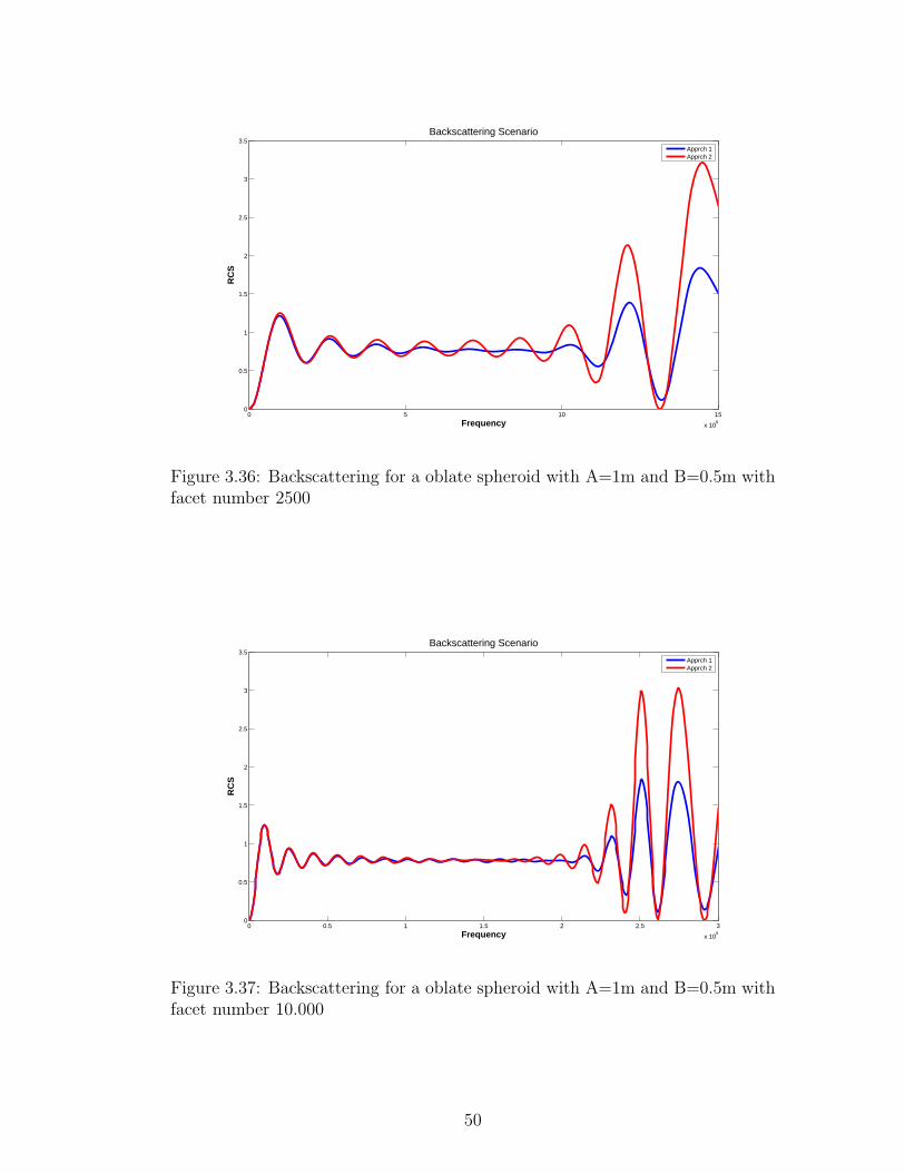
For the first two figures, simulations are done for a oblate spheroid. A = 1m

is the radius in x and y direction. B = 0.5m is the radius in z direction in this

case. In figures (3.36) and (3.37), facet numbers are 2500 and 10.000 respectively.

And as expected, boundary frequency values between second and third regions

43

0 20 40 60 80 100 120 140 16010

0

101

102

φ (Degrees)

RC

S

Bistatic Backscattering Scenario


Figure 3.25: Bistatic scenario: φ polarized incident wave with facet number of1024

0 20 40 60 80 100 120 140 16010

−4

10−3

10−2

10−1

100

101

102

φ (Degrees)

RC

S

Bistatic Scattering Scenario


Figure 3.26: Bistatic scenario: θ polarized incident wave with facet number of1024

44

0 20 40 60 80 100 120 140 16010

0

101

102

φ (Degress)

RC

S




0 20 40 60 80 100 120 140 16010

−4

10−3

10−2

10−1

100

101

102

φ (Degrees)

RC

S




45

0 20 40 60 80 100 120 140 16010

0

101

102

φ (Degrees)

RC

S




0 20 40 60 80 100 120 140 16010

−4

10−3

10−2

10−1

100

101

102

φ (Degrees)

RC

S




46

0 20 40 60 80 100 120 140 16010

0

101

102

103

φ in degrees

Bis

tati

c R

CS

Bistatic Scenario σφφ


Figure 3.31: Bistatic scenario: φ polarized incident wave with facet number of10.000 at 900MHz

0 20 40 60 80 100 120 140 16010

−1

100

101

102

103

Bistatic Scenario σθθ

Bis

tati

c R

CS

φ in degrees


Figure 3.32: Bistatic scenario: θ polarized incident wave with facet number of10.000 at 900MHz

47

0 20 40 60 80 100 120 140 16010

0

101

102

103

φ in degrees

Bis

tati

c R

CS

Bistatic Scenario σφφ


Figure 3.33: Bistatic scenario: φ polarized incident wave with facet number of62.500 at 900MHz

0 20 40 60 80 100 120 140 16010

−1

100

101

102

103

Bistatic Scenario σθθ

Bis

tati

c R

CS

φ in degrees


Figure 3.34: Bistatic scenario: θ polarized incident wave with facet number of62.500 at 900MHz

48

Figure 3.35: Backscattering scenario for scattering from ellipsoid

are increased by number of facets. For sphere case, converged value is the cross

sectional area of the sphere, however for this time, results are different. Cross

sectional area of an ellipse is given as Area = πAB. Therefore, area of this oblate

spheroid is πAB = 1.570 m2. However, echo area in GO region is even less than

1. Due to GO, reflection depends on the radius of curvature at the specular

point. This issue will be investigated thoroughly in another section.

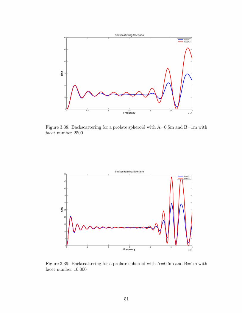
For the prolate spheroid case, A = 0.5 is the radius in x axis, B = 1 is the

radius in y and z axes. The cross sectional area is the same with a unit sphere,

however, results in GO region is more than 15. Figures (3.38) and (3.39) show

the results of the simulations for this oblate spheroid with 2500 and 10.000 facets

respectively.

49

0 5 10 15

x 108

0

0.5

1

1.5

2

2.5

3

3.5

Frequency

RC

S


Apprch 1Apprch 2

Figure 3.36: Backscattering for a oblate spheroid with A=1m and B=0.5m withfacet number 2500

0 0.5 1 1.5 2 2.5 3

x 109

0

0.5

1

1.5

2

2.5

3

3.5Backscattering Scenario

RC

S

Frequency

Apprch 1Apprch 2

Figure 3.37: Backscattering for a oblate spheroid with A=1m and B=0.5m withfacet number 10.000

50

0 0.5 1 1.5 2 2.5 3

x 109

0

10

20

30

40

50

60Backscattering Scenario

RC

S

Frequency

Apprch 1Apprch 2

Figure 3.38: Backscattering for a prolate spheroid with A=0.5m and B=1m withfacet number 2500

0 1 2 3 4 5 6

x 109

0

5

10

15

20

25

30

35

40

45


RC

S

Frequency

Apprch 1Apprch 2

Figure 3.39: Backscattering for a prolate spheroid with A=0.5m and B=1m withfacet number 10.000

51

3.2.4 Case 4: Special Comparison Regarding the Radius

of Curvature in GO Calculation

Reflected power in GO depends on the radius of curvature at the specular point.

Radius of curvature of a spheroid at the point on the axial direction may be

calculated by the following formula [2]:

R(u) = −(B2 cos2 u + A2 sin2 u)3/2

AB(3.1)

u is the angle between x axis and the line connecting the origin and the point

we desire to find the radius of curvature at. A and B are defined in figure

(3.35) already. Thinking of a prolate spheroid with radii A = 1m at x axis and

B = 0.5m at y and z axes. Incident field is assumed to come from +x direction.

Therefore, at specular point, radius of curvature is calculated as R = 14

m. Due

to GO, RCS of a sphere of radius 14

m should be equal to this prolate spheroid.

For oblate spheroid case, A = 0.5m on x axis and B = 1m for y and z axes.

At this time, radius of curvature at the specular point is 2m. Comparisons of

these two cases are in figures (3.40), (3.41),(3.42) and (3.43). Number of facets

is 10.000 for all simulations at this section.

As seen in figures, our calculations are consistent with the GO. However,

the critical frequency value changes between spheres and ellipsoids having the

same radius of curvature. For instance, the critical value for the oblate spheroid

(Figure (3.40)) is about 2GHz, whereas the same value (Figure(3.41)) is about

8GHz for the sphere which has the same radius of curvature. Similarly, critical

frequency value in figure (3.42) is about four times greater than that value in

(3.43). Since that critical frequency depends on the size of a facet and for all these

simulations, total number of facets is constant, the sphere or ellipsoid which is

smaller, namely the ones whose facets are smaller, has this value much less than

the other. In figure (3.44), a simulation is performed using a sphere with radius

52

0 0.5 1 1.5 2 2.5 3

x 109

0

0.1

0.2

0.3

0.4

0.5

0.6

0.7


Frequency

RC

S

Figure 3.40: Backscattering for a oblate spheroid with A=1m and B=0.5m

0 2 4 6 8 10 12

x 109

0

0.1

0.2

0.3

0.4

0.5

0.6

0.7


RC

S

Frequency

Apprch 1Apprch 2

Figure 3.41: Backscattering for a sphere with radius R=1/4

53

0 1 2 3 4 5 6

x 109

0

5

10

15

20

25

30

35

40

45


Frequency

RC

S

Apprch 1Apprch 2

Figure 3.42: Backscattering for a prolate spheroid with A=0.5m and B=1m

0 0.2 0.4 0.6 0.8 1 1.2 1.4 1.6 1.8 2

x 109

0

10

20

30

40

50


RC

S

Frequency

Apprch 1Apprch 2

Figure 3.43: Backscattering for a sphere with radius R=2

54

0 1 2 3 4 5 6

x 109

0

5

10

15

20

25

30

35

40

45

50

Frequency

RC

S


Apprch 1Apprch 2

Figure 3.44: Backscattering for a sphere with radius R=2 with excess facets

of 2m as in figure (3.43). At this time, dimension of a single facet is the same as

the prolate spheroid in figure (3.42). It is observed that critical frequency value

is the same.

3.2.5 Case 5: Usability Analysis of PO Approaches

In this case, a series of simulations are performed in order to obtain an idea

about modeling curved surfaces and application of the PO. Since curved surfaces

are modeled with planar triangular facets, they are actually not curved surfaces

in the simulations any more (ie. a perfect sphere or a football). Using large

number of facets and small operation frequencies, the difference between a sphere

and a football may be invisible for our calculations. However, as the frequency

increases, these differences become more and more visible and cause the results

deviate from the theoretical GO, ie RCS of a sphere is its cross sectional area in

high frequency region.

The critical frequency that the deviation begins is clearly a function of dimen-

sion of the facets used in modeling. In this case, these critical frequency values

55

0 1 2 3 4 5 6 7 8

x 105

0.19

0.2

0.21

0.22

0.23

0.24

0.25Backscattering Scenario for the sphere (Special Case)

Rat

io b

tw t

he

dim

ensi

on

of

a fa

cet

and

wav

elen

gth

Number of Facets

Apprch 1Apprch 2

Figure 3.45: Number of facets vs dimension of a facet at the critical frequency

are recorded and plotted with respect to the dimension of a facet. In defining

the values, 5 percent deviation is taken as the criteria. Also, a plot is generated

in which one has the opportunity to compare the ratio between the dimension of

a facet and the operation wavelength versus the total number of facets.

It is seen in figures (3.45) and (3.46), the dependence of accuracy of the

approaches to the dimension of a single facet is not linear as expected. Increasing

the number of facets, the model gets better, faster than the speed of dimension’s

getting smaller.

A similar simulation is performed in order to link the radius of curvature to

the critical frequency. In figure (3.47), it is seen that for constant number of

facets (10.000 in this case) increasing the radius decreases the critical frequency.

However, for small values, a unit decrease in curvature effects this limit more

than for respectively large values. This result is consistent with the previous

ones. Since the radius increases as the total number of facets is fixed, modelling

accuracy decreases.

56

Figure 3.46: Dimension of facet vs critical frequency

0 5 10 15 20 25 30 35 40 45 500

0.5

1

1.5

2

2.5

3

3.5

4

4.5x 10

9 Critical Frequency vs Radius of Curvature

Cri

tica

l fre

qu

ency

du

e to

5%

Cri

teri

a in

Hz

Raduis of Curvature in m

Apprch 1Apprch 2

Figure 3.47: Radius of curvature for constant facet number vs critical frequency

57

0 0.5 1 1.5 2 2.5 3

x 104

0

10

20

30

40

50

60

70

Number of facets

Tim

e fo

r im

ple

men

tati

on

in m

inu

tes

Time consuption analysis of approaches

Apprch 1Apprch 25−point Gaussian Quadrature

Figure 3.48: Time consumption of approaches

3.2.6 Case 6: Time Consumption Analysis of Approaches

In this case, time consumption analysis is done for two approaches and another

technique for numerical integration which is called, Gaussian quadrature. 5-point

Gaussian is used in the simulations. As seen in figure (3.48), time consumed by

Approach 1 is quite larger than Approach 2 whereas the accuracy is not that

much better. On the other hand, Gaussian quadrature method takes acceptable

time, however results are less precise than both approaches.

58

Chapter 4

CONCLUSIONS

In this work, a computer program which uses Physical Optics (PO) method

to calculate the RCS of perfectly conducting planar and spherical structures is

developed. MATLAB is used as the high-level computing tool. The target bodies

are modeled with triangular meshes. The program includes a mesh generation

algorithm.

PO which is one of the high frequency techniques, approximates the induced

surface currents predicted by GO and integrates them over the surface in order

to calculate total scattered field. Two approaches are introduced in this work for

calculating this radiation surface integral.

In the first approach, the PO integral is calculated analytically and this ana-

lytical solution is used. However, for curved surfaces, using large pieces damages

the modeling accuracy; therefore results may differ widely from exact solutions.

On the other hand, applying analytical solution instead of taking the integral

directly lessens the computational cost and makes the computation much faster

than Method of Moments solution.

59

However, there exists another approach which has much less computation

cost than the previous one. In this second approach, phase difference within

a facet is assumed to be constant. Namely, a single facet has an area but is

considered as a point in phase calculation point of view. However by this way,

the accuracy of this approach becomes dependant on the size of the meshes.

Larger meshes deviate the result from both results of first approach and from

Method of Moments solution.

In this study, a comprehensive comparison has been carried out for several

conditions. For plate geometries, for the case the observation is the specular

direction, since phase is not an issue within a facet, two approaches does not

differ. Similarly, since spheres are modeled using flat facets, forward scattering

power is independent of PO integral approach.

For all simulations, the unchanged truth is that, increasing the number of

facets two approaches put closer results out. This fact is independent from

geometry, frequency of operation or any other variable. On the other hand,

results of Approach 1 are independent of number of facets used in modeling

for plate geometries but dependent for spheres. For a certain frequency, more

deviation from specular aspect makes results of the approaches more apart. This

is because the phase difference between any two facets and within a facet gets

more.

For plate geometries (squares and rectangles), for fixed difference between

results at a particular aspect angle (backscattering aspect), maximum operation

frequency increases by number of facets and by incident angle (getting closer to

normal incidence). This is because the phase difference lessens.

For rectangles, keeping the facet size constant, increasing one dimension of the

plate causes more oscillations which is expected due to increase in the number of

reflectors (facets). A simulation for certain and different incident and observation

60

angles and varying frequency is performed. It is observed that, all null points

in the results of both approaches coincide. Due to interference, scattered power

shows an oscillatory behavior and as the frequency increases two approaches

differ from each other for a certain number of facets.

For spheres, backscattering and bistatic scattering scenarios have been per-

formed. For backscattering case, frequency is the variable for each simulation.

For very high frequencies, PO gives erroneous results because asymptotic ap-

proximation fails since ratio between an edge of a facet and wavelength exceeds

a limit. In the simulations, this limit is designated as a function of dimension

of facets. Namely, as the frequency gets higher and higher, difference between a

perfect sphere and a meshed model becomes observable.

Simulations for ellipsoids are performed for oblate and prolate spheroids. Ac-

cording to the GO, RCS of a scatterer is a function of the radius of curvature

at the specular point. In this case, oblate and prolate spheroids are compared

with the spheres having the same radius of curvature and facet number. It is

shown that our implementation is true for backscattering case. Also, regarding

the critical frequency value, (the boundary value between GO and PO diffrac-

tion regions, see section 3.2.1) a sphere of the same radius of curvature with the

spheroid and the dimension of a facet, is compared and observed that this critical

value is a function of dimension of the facets used in modeling. This function is

tried to be determined by a simple application. The frequency values at which

the results deviate from the GO for a certain amount are recorded. It is observed

that, critical frequency is inversely proportional with the square of dimension of

the facet.

To conclude, the PO is computationally very advantageous in comparison

with the Method of Moments and it gives very good results around specular

direction. Among these approaches, for flat surfaces, Approach 1 is better. Be-

cause, in order to have close results, Approach 2 needs very large number of facets

61

so much computational cost. However, for curved surfaces, Approach 2, since it

gives quite good results in about one fourth of the time spent by Approach 1, is

preferable.

62

Bibliography

[1] R. Harrington, “Time-Harmonic Electromagnetic Fields,” McGraw-Hill,

vol. 33, p. 34, 1961.

[2] D. McNamara, C. Pistorius, and J. Malherbe, Introduction to the uniform

geometrical theory of diffraction. Artech House Boston, 1990.

[3] P. Pathak, “Techniques for high frequency problems,” Antenna Handbook,

pp. 96–115, 1988.

[4] W. Gordon, “High frequency approximations to the physical optics scat-

teringintegral,” Antennas and Propagation, IEEE Transactions on, vol. 42,

no. 3, pp. 427–432, 1994.

[5] V. Stein, “Application of Equivalent Edge Currents to Correct the Backscat-

tered Physical Optics Field of Flat Plates,” Applied Computational Electro-

magnetics Society Journal, vol. 7.

[6] R. Ross, “Radar cross section of rectangular flat plates as a function of

aspect angle,” Antennas and Propagation, IEEE Transactions on [legacy,

pre-1988], vol. 14, no. 3, pp. 329–335, 1966.

[7] C. Balanis, Antenna theory. Wiley New York, 1997.

[8] E. Knott, M. Tuley, and J. Shaeffer, “Radar Cross Section,” 2003.

[9] J. Richmond, “A COMPUTER PROGRAM FOR PHYSICAL-OPTICS

SCATTERING BY CONVEX CONDUCTING TARGETS.,” 1968.

63

[10] B. Tiryaki, “Solution with method of moments,” Personal Communication,

2008.

64

COMPARISON OF TWO PHYSICAL OPTICS ... OF TWO PHYSICAL OPTICS INTEGRATION APPROACHES FOR...

Documents

Transcript of COMPARISON OF TWO PHYSICAL OPTICS ... OF TWO PHYSICAL OPTICS INTEGRATION APPROACHES FOR...