KULeuven Energy Institute

TME Branch

WP EN2012-006

Comparison of Thermodynamic Cycles for Electricity Production

from Low-Temperature Geothermal Heat Sources

Daniël Walraven, Ben Laenen en William D'haeseleer

TME WORKING PAPER - Energy and Environment Last update: April 2012

An electronic version of the paper may be downloaded from the TME website:

http://www.mech.kuleuven.be/tme/research/

Comparison of Thermodynamic Cycles for Electricity Production

from Low-Temperature Geothermal Heat Sources

Daniel Walravena, Ben Laenenb, William D’haeseleera

a University of Leuven (KU Leuven) Energy Institute - TME branch (Applied Mechanics and Energy

Conversion), Celestijnenlaan 300A box 2421, B-3001 Leuven, Belgium

b Flemish Institute of Technological Research (VITO),

Boeretang 200, B-2400 Mol, Belgium

E-mail addresses: daniel.walraven@mech.kuleuven.be, ben.laenen@vito.be, william.dhaeseleer@mech.kuleuven.be

Abstract

The performance of different types of organic Rankine cycles (ORC) and of the Kalinacycle is investigated for low-temperature (100-150◦C) geothermal heat sources. A varietyof configurations is worth considering. The ORC’s can be subcritical or transcritical andcan have one or more pressure levels. Each cycle can be a standard one, have recuperationor turbine bleeding. Comparison of these cycles concludes that the transcritical and multi-pressure subcritical cycles are the best ones. Exergetic plant efficiencies of above 50% canbe achieved when the brine is allowed to cool down as much as possible. A limit on thebrine outlet temperature causes a strong decrease in the mechanical power output of thecycle. Due to the low heat source temperatures, a low condenser temperature and smalltemperature differences in the heat exchanger are important.

Keywords: Geothermal, ORC, Kalina

1 Introduction

Low-temperature (100-150◦C) geothermal heat sources have a very large potential as a renewableenergy source [1, 2]. The amount of energy available is huge, but due to the low-temperature,the electricity conversion efficiency is low. For this energy conversion, two types of cycles areproposed in the literature. The first one is the organic Rankine cycle (ORC), which is similarto a steam Rankine cycle, but uses an organic working fluid instead of water. A second type isthe so-called Kalina cycle. ORC’s are used for different low-temperature heat sources (biomass,geothermal, solar, ...) [3].

Different configurations have been proposed in the literature. Cayer et al. [4] have optimizeda transcritical ORC for a heat-source temperature of 100◦C. CO2, ethane and R125 are usedas possible working fluids. Only the simple ORC configuration with a pump, heat exchanger,turbine and condenser are considered. Kanoglu [5] has investigated multi-pressure cycles. Anexergy analysis of an existing power plant, which uses the combination of 2 subcritical cycleswith isopentane, has been performed. Gnutek and Bryszewska-Mazurek [6] have considered amulti-cycle ORC. The power plant consists of 4 subcritical power cycles, using the heat source

1

in series. Heberle and Bruggemann [7] have concluded that for power generation from low-temperature geothermal heat sources, fluids with a low critical temperature are optimum. Onlycycles which use a recuperator have been investigated. Mago et al. [8] have compared stan-dard ORC’s with ORC’s which use turbine bleeding (called ”regenerative” in the paper). Itis concluded that the cycle efficiency of the so-called regenerative cycle is higher than that ofthe standard cycle. Different configurations of subcritical ORC’s have been compared by Yari[9]. Standard cycles, cycles with recuperation, cycles with turbine bleeding and cycles withrecuperation and turbine bleeding are simulated. It is shown that cycles with recuperationor turbine bleeding are the most promising ones. Subcritical and transcritical cycles with orwithout recuperation have been investigated by Saleh et al. [10] for many working fluids. Forlow-temperature geothermal sources, it is shown that fluids with a low critical pressure in thetranscritical cycles are optimum.

For low-temperature sources, the Kalina is often mentioned as an alternative for the ORC.The Kalina cycle is similar to an ORC, but uses a mixture of water and ammonia with avariable composition as working fluid [11–13]. Although the Kalina cycle is often called to besuperior to the ORC, DiPippo [14] has shown that an existing Kalina cycle has about the sameperformance as existing ORC’s.

In this paper different types of ORC’s and the Kalina cycle are thermodynamically optimizedand compared, but only pure fluids are used for the ORC’s. In section 2, different types ofefficiencies are defined and compared to each other. Energetic and exergetic efficiencies for theplant and the thermodynamic cycle are defined. In the third section, different cycle configura-tions are described for the ORC’s and the Kalina cycle. In section 4, these configurations areoptimized using different organic fluids for different cases. The influence of some parameters isinvestigated.

2 Definition of Different Efficiencies

In the literature, different definitions for efficiencies exist. All of these efficiencies are useful,but they often have a different meaning. Therefore, it is important to know how the efficienciesare defined and to use the right efficiency at the right moment.

2.1 Cycle Efficiency

The cycle efficiency describes how well a thermodynamic cycle converts heat, which is addedto the cycle, to mechanical power. The energetic cycle efficiency is defined as the fraction ofthe net mechanical power output to the heat input:

ηcycleen =Wnet

Qin

(1)

Wnet and Qin are the net mechanical power output and the heat input to the cycle, respectively.When the heat source is a geothermal brine, the heat added to the cycle can be written as

Qin = mbrine∆hbrine = mbrine(hin − hout) (2)

with mbrine the mass flow of brine, ∆hbrine the specific enthalpy drop of the brine, hin and houtthe specific enthalpy of the brine before and after heat is added to the cycle. So, equation (1)can be written as:

ηcycleen =Wnet

mbrine(hin − hout)(3)

2

Analogous to the energetic cycle efficiency, also an exergetic cycle efficiency can be defined:

ηcycleex =Wnet

mbrine(ein − eout)(4)

where ein and eout are the specific flow exergy of the brine before and after heat is added to thecycle, respectively. The specific flow exergy is defined as:

e = (h− h0)− T0(s− s0), (5)

where s is the specific entropy of the brine and the subscript 0 refers to the dead state; so T0 isthe dead-state temperature, usually being the temperature of the environment. The advantageof the exergetic cycle efficiency is that it is the fraction of real work output to the maximumobtainable output and therefore is an indication how far away the cycle is from the ideal one.

2.2 Plant Efficiency

The cycle efficiency of the previous section only describes how efficient a cycle is in converting acertain amount of heat into mechanical power, but it does not tell how efficient the heat sourceis used. Therefore, both energetic and exergetic plant efficiencies are defined, respectively:

ηplanten =Wnet

Qavailable

=Wnet

mbrine(hin − h0)(6)

ηplantex =Wnet

Eavailable

=Wnet

mbrineein(7)

Qavailable and Eavailable are the heat and exergy in the heat source, respectively. The differencewith Eqs. (3) and (4) is that hout and eout have been replaced by h0 and e0 = 0, respectively.These plant efficiencies can be rewritten in function of the respective cycle efficiencies:

ηplanten =Wnet

mbrine(hin − hout)mbrine(hin − hout)mbrine(hin − h0)

(8)

= ηcycleen ηcoolingen (9)

(10)

ηplantex =Wnet

mbrine(ein − eout)mbrine(ein − eout)

mbrineein(11)

= ηcycleex ηcoolingex (12)

where ηcoolingen and ηcoolingex show how efficient the geothermal brine is cooled in the energetic andexergetic sense, respectively.

When a geothermal brine is used to produce electricity, the goal is to maximize the net work

output per mass unit of brine. So, the fraction Wnetmbrine

should be maximized. As seen from Eqs.(6) and (7) this is the same as maximizing the energetic or exergetic plant efficiency, becausehin, h0 and ein only depend on the geothermal source and the environment.

Equations (9) and (12) show that the heat source should be cooled down as far as possible

(i.e., ηcoolingi → 1) and the heat added to the cycle should be efficiently converted to electricity,to have a high plant efficiency and thus a high power output per mass unit of brine.

In this paper, different configurations of Organic Rankine Cycles (ORC’s) and the Kalina cyclewill be described and optimized for maximum plant efficiency.

3

3 Organic Rankine Cycle

The Organic Rankine Cycle (ORC) is a Rankine cycle with an organic working fluid. Manyorganic fluids have lower critical temperatures than water and are better suited for powerproduction from low-temperature heat sources. In this section, different types of ORC’s aredescribed.

3.1 Subcritical and Transcritical ORC’s

A distinction has to be made between subcritical, transcritical and supercritical cycles. In asubcritical cycle, the pressure is always below the critical pressure and in a supercritical cycle,the pressure is always above the critical pressure. In a transcritical cycle, the low pressure isbelow the critical pressure, and the high pressure above the critical one1. In this paper, onlysubcritical and transcritical cycles are investigated.

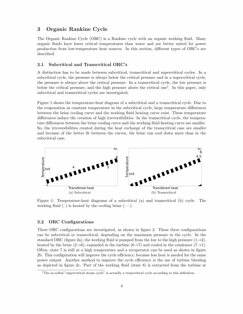
Figure 1 shows the temperature-heat diagram of a subcritical and a transcritical cycle. Due tothe evaporation at constant temperature in the subcritical cycle, large temperature differencesbetween the brine cooling curve and the working fluid heating curve exist. These temperaturedifferences induce the creation of high irreversibilities. In the transcritical cycle, the tempera-ture differences between the brine cooling curve and the working fluid heating curve are smaller.So, the irreversibilities created during the heat exchange of the transcritical case are smallerand because of the better fit between the curves, the brine can cool down more than in thesubcritical case.

(a) Subcritical (b) Transcritical

Figure 1: Temperature-heat diagrams of a subcritical (a) and transcritical (b) cycle. Theworking fluid (–) is heated by the cooling brine (· · · ).

3.2 ORC Configurations

Three ORC configurations are investigated, as shown in figure 2. These three configurationscan be subcritical or transcritical, depending on the maximum pressure in the cycle. In thestandard ORC (figure 2a), the working fluid is pumped from the low to the high pressure (1→2),heated by the brine (2→6), expanded in the turbine (6→7) and cooled in the condenser (7→1).Often, state 7 is still at a high temperature and a recuperator can be used as shown in figure2b. This configuration will improve the cycle efficiency, because less heat is needed for the samepower output. Another method to improve the cycle efficiency is the use of turbine bleedingas depicted in figure 2c. Part of the working fluid (state 8) is extracted from the turbine at

1The so-called ”supercritical steam cycle” is actually a transcritical cycle according to this definition.

4

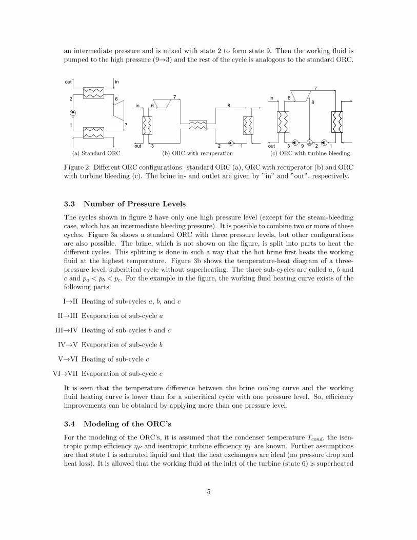
an intermediate pressure and is mixed with state 2 to form state 9. Then the working fluid ispumped to the high pressure (9→3) and the rest of the cycle is analogous to the standard ORC.

2 6

1 7

inout

(a) Standard ORC

3

6

7

in

out 2 1

8

(b) ORC with recuperation

2

6

1

7

in

out 93

8

(c) ORC with turbine bleeding

Figure 2: Different ORC configurations: standard ORC (a), ORC with recuperator (b) and ORCwith turbine bleeding (c). The brine in- and outlet are given by ”in” and ”out”, respectively.

3.3 Number of Pressure Levels

The cycles shown in figure 2 have only one high pressure level (except for the steam-bleedingcase, which has an intermediate bleeding pressure). It is possible to combine two or more of thesecycles. Figure 3a shows a standard ORC with three pressure levels, but other configurationsare also possible. The brine, which is not shown on the figure, is split into parts to heat thedifferent cycles. This splitting is done in such a way that the hot brine first heats the workingfluid at the highest temperature. Figure 3b shows the temperature-heat diagram of a three-pressure level, subcritical cycle without superheating. The three sub-cycles are called a, b andc and pa < pb < pc. For the example in the figure, the working fluid heating curve exists of thefollowing parts:

I→II Heating of sub-cycles a, b, and c

II→III Evaporation of sub-cycle a

III→IV Heating of sub-cycles b and c

IV→V Evaporation of sub-cycle b

V→VI Heating of sub-cycle c

VI→VII Evaporation of sub-cycle c

It is seen that the temperature difference between the brine cooling curve and the workingfluid heating curve is lower than for a subcritical cycle with one pressure level. So, efficiencyimprovements can be obtained by applying more than one pressure level.

3.4 Modeling of the ORC’s

For the modeling of the ORC’s, it is assumed that the condenser temperature Tcond, the isen-tropic pump efficiency ηP and isentropic turbine efficiency ηT are known. Further assumptionsare that state 1 is saturated liquid and that the heat exchangers are ideal (no pressure drop andheat loss). It is allowed that the working fluid at the inlet of the turbine (state 6) is superheated

5

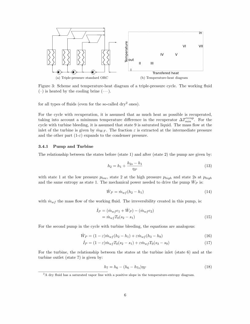
(a) Triple-pressure standard ORC (b) Temperature-heat diagram

Figure 3: Scheme and temperature-heat diagram of a triple-pressure cycle. The working fluid(–) is heated by the cooling brine (· · · ).

for all types of fluids (even for the so-called dry2 ones).

For the cycle with recuperation, it is assumed that as much heat as possible is recuperated,taking into account a minimum temperature difference in the recuperator ∆T recup

min . For thecycle with turbine bleeding, it is assumed that state 9 is saturated liquid. The mass flow at theinlet of the turbine is given by mWF . The fraction ε is extracted at the intermediate pressureand the other part (1-ε) expands to the condenser pressure.

3.4.1 Pump and Turbine

The relationship between the states before (state 1) and after (state 2) the pump are given by:

h2 = h1 +h2s − h1ηP

(13)

with state 1 at the low pressure plow, state 2 at the high pressure phigh and state 2s at phighand the same entropy as state 1. The mechanical power needed to drive the pump WP is:

WP = mwf (h2 − h1) (14)

with mwf the mass flow of the working fluid. The irreversibility created in this pump, is:

IP = (mwfe1 + WP )− (mwfe2)

= mwfT0(s2 − s1) (15)

For the second pump in the cycle with turbine bleeding, the equations are analogous:

WP = (1− ε)mwf (h2 − h1) + εmwf (h3 − h9) (16)

IP = (1− ε)mwfT0(s2 − s1) + εmwfT0(s3 − s9) (17)

For the turbine, the relationship between the states at the turbine inlet (state 6) and at theturbine outlet (state 7) is given by:

h7 = h6 − (h6 − h7s)ηT (18)

2A dry fluid has a saturated vapor line with a positive slope in the temperature-entropy diagram.

6

with state 6 at phigh, state 7 at plow and state 7s at plow and the same entropy as state 6. Theturbine mechanical power and irreversibility generated in the turbine are:

WT = mwf (h6 − h7) (19)

IT = mwfT0(s7 − s6) (20)

For the cycle with turbine bleeding, these equations are:

WT = mwf (h6 − h8) + (1− ε)mwf (h8 − h7) (21)

IT = mwfT0(s8 − s6) + (1− ε)mwfT0(s7 − s8) (22)

In this paper, the net mechanical power output is given by:

Wnet = WT − WP (23)

So, the power needed for cooling and other auxiliary power is not taken into account.

3.4.2 Heat exchangers

The heat exchangers are assumed to be ideal; so no pressure drop is induced and no heat islost to the environment. The energy balance for the heat exchanger HX between the brine andworking fluid is given by:

mbrine(hin − hout) = mwf (h6 − h3) (24)

A fixed pinch point temperature difference ∆THXmin is assumed in this heat exchanger. In the

recuperator, the energy balance is:

(h7 − h8) = (h3 − h2) (25)

and the minimum temperature difference is given by ∆T recupmin . The pinch point temperature dif-

ferences ∆THXmin and ∆T recup

min are generally not the same. The energy equation for the condenserin the standard or recuperated cycle is given by

mwf (hx − h1) = mcooling(hcoolingout − hcoolingin ) (26)

with hx = h7 in the standard cycle and hx = h8 in the cycle with recuperator. The pinch pointtemperature difference in the condenser is ∆T condenser

min , a mass flow mcooling of cooling water is

used and hcoolingin & hcoolingout are the enthalpy of the cooling water before and after the condenser,respectively.

The irreversibilities created in the HX and recuperator are:

IHX = (mbrineein + mwfe3)− (mbrineeout + mwfe6)

= mbrineT0(sout − sin) + mwfT0(s6 − s3) (27)

Irecup = mwf [(e2 + e7)− (e3 + e8)]

= mwfT0[(s3 − s2) + (s8 − s7)] (28)

(29)

The irreversibilities created in the cooling installation are given by

Icool = mwf (ex − e1) (30)

with ex = e7 for the standard cycle and ex = e8 for the cycle with recuperation. So, inthe cooling installation, all the exergy is lost to the environment. For the cycle with turbinebleeding, the irreversibility creation is:

Icool = (1− ε)mwf (e7 − e1) (31)

7

3.4.3 Mixing

In the cycle with turbine bleeding, two flows are mixed. The energy equation for the mixingprocess is given by:

εh8 + (1− ε)h2 = h9 (32)

and the irreversibility created is:

Imix = mwf ([(1− ε)e2 + εe8]− e9)= mwfT0(s9 − [(1− ε)s2 + εs8]) (33)

4 Kalina Cycle

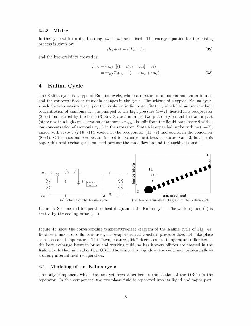
The Kalina cycle is a type of Rankine cycle, where a mixture of ammonia and water is usedand the concentration of ammonia changes in the cycle. The scheme of a typical Kalina cycle,which always contains a recuperator, is shown in figure 4a. State 1, which has an intermediateconcentration of ammonia xint, is pumped to the high pressure (1→2), heated in a recuperator(2→3) and heated by the brine (3→5). State 5 is in the two-phase region and the vapor part(state 6 with a high concentration of ammonia xhigh) is split from the liquid part (state 9 with alow concentration of ammonia xlow) in the separator. State 6 is expanded in the turbine (6→7),mixed with state 9 (7+9→11), cooled in the recuperator (11→8) and cooled in the condenser(8→1). Often a second recuperator is used to exchange heat between states 9 and 3, but in thispaper this heat exchanger is omitted because the mass flow around the turbine is small.

3

6 7in

out 2 1

85

9 11

(a) Scheme of the Kalina cycle. (b) Temperature-heat diagram of the Kalina cycle.

Figure 4: Scheme and temperature-heat diagram of the Kalina cycle. The working fluid (–) isheated by the cooling brine (· · · ).

Figure 4b show the corresponding temperature-heat diagram of the Kalina cycle of Fig. 4a.Because a mixture of fluids is used, the evaporation at constant pressure does not take placeat a constant temperature. This ”temperature glide” decreases the temperature difference inthe heat exchange between brine and working fluid; so less irreversibilities are created in theKalina cycle than in a subcritical ORC. The temperature-glide at the condenser pressure allowsa strong internal heat recuperation.

4.1 Modeling of the Kalina cycle

The only component which has not yet been described in the section of the ORC’s is theseparator. In this component, the two-phase fluid is separated into its liquid and vapor part.

8

An amount mwf of working fluid is heated in the heat exchanger, the fraction ε of this massflow is expanded in the turbine:

ε =xint − xlowxhigh − xlow

(34)

5 Results and Discussion

In this section, the results of the comparison between the ORC configurations of Figs. 2 & 3and the Kalina cycle of Fig. 4 for the different cases are given. All the simulations have beenperformed with our own developed code, written in Python. The thermodynamic propertiesare obtained from RefProp [15].

5.1 Input Parameters

Table 1 shows the parameters which are used in the remainder of this paper, unless denotedotherwise. The brine inlet temperature and pressure are given by Tin and pin, respectively. Thecooling water temperature is taken equal to T0.

Tin 125◦Cpin 5 bar

Tcond 25◦CT0 15◦Cp0 1 bar

ηP 80 %

ηT 85 %

∆THXmin 5◦C

∆T recupmin 5◦C

∆T condmin 5◦C

Table 1: Input parameters.

For some fluids available in RefProp, only supercritical cycles are possible and they are thereforeskipped. All other fluids, even those which are legally prohibited, are used in the calculationsto obtain the thermodynamic optimum cycle configuration. For the Kalina cycle, a maximumammonia concentration of 96% is used, because for higher concentrations RefProp is not alwaysable to find the thermodynamic properties of the mixture.

5.2 Net Power Output

In this section, two cases are investigated. In the first case, there is no limit on the brine outlettemperature. In the second case, a minimum brine outlet temperature of 75◦C is used. This isdone to simulate cases where scaling (fouling) has to be avoided or when the brine is used forheating or cooling (absorption or adsorption cooling).

5.2.1 Brine cooling temperature without limit

a Single pressure

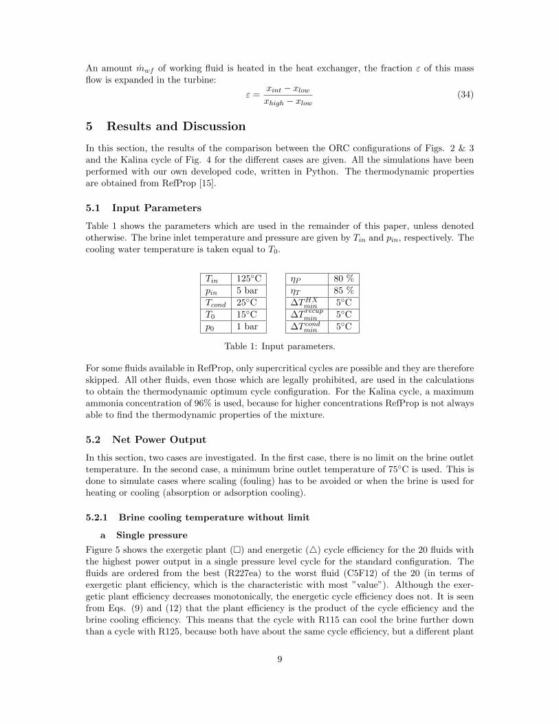
Figure 5 shows the exergetic plant (�) and energetic (4) cycle efficiency for the 20 fluids withthe highest power output in a single pressure level cycle for the standard configuration. Thefluids are ordered from the best (R227ea) to the worst fluid (C5F12) of the 20 (in terms ofexergetic plant efficiency, which is the characteristic with most ”value”). Although the exer-getic plant efficiency decreases monotonically, the energetic cycle efficiency does not. It is seenfrom Eqs. (9) and (12) that the plant efficiency is the product of the cycle efficiency and thebrine cooling efficiency. This means that the cycle with R115 can cool the brine further downthan a cycle with R125, because both have about the same cycle efficiency, but a different plant

9

efficiency. The other way around is also possible, as seen with R41 and R32.

R22

7eaS

R11

5S

R12

5S

R14

3aS

R21

8S

R12

34yf S

R41

S

R32

S

N2O

S

SF

6S

Propylene S

C4F

10S

Propane S

RC

318 S

R13

4aS

CO

2S

R12

34ze

S

EthaneS

R23

6faS

C5F

12S40

45

50

55

60ηplant

ex[%

]ηplantex

ηcycleen

9.0

9.5

10.0

10.5

11.0

11.5

12.0

12.5

ηcycle

en[%

]

Figure 5: Exergetic plant efficiency and energetic cycle efficiency of the 20 fluids with the highestmechanical power output in a single pressure level cycle for the standard (S) configuration.Subcritical cycles are denoted with a subscript S and transcritical cycles with a superscript S.

In this figure, only cycles with a standard configuration are shown, because the model showsthat it is not useful to use a recuperator or turbine bleeding. Recuperation and turbine bleedingcan increase the cycle efficiency, but not the plant efficiency in this case. When an internal heatexchanger is used, the amount of heat transfered between the brine and the working fluid isdecreased and the brine cools down less. The cycle efficiency increases, but the brine coolingefficiency decreases. The net result is zero.

All pure fluids condense at a constant temperature, so that the cooling water temperatureincreases to about 20◦C (Tcond−∆T cond

min ). In the Kalina cycle, the minimum temperature in thecondenser is assumed to be 21◦C instead of 25◦C, so that the cooling water heats up from 15 toabout 20◦C. Even with this assumption, the exergetic plant efficiency of the Kalina cycle is only41.5%. So, the Kalina cycle is even thermodynamicaly outperformed by standard subcriticalORC’s. The obtained Kalina cycle, is not a ”real” Kalina cycle, because the working fluid be-fore the separator (state 5) is saturated vapor. So, a separator is not needed and a recuperatedsubcritical ORC with a mixture of water and ammonia with a constant concentration is obtained.

In the Kalina cycle, the temperature glide at the condenser pressure allows a high amountof recuperation. As shown in figure 4b, the pinch point is somewhere in the evaporator and notat the end of the economizer. This allows a higher mass flow of working fluid per unit brineand a higher power output.

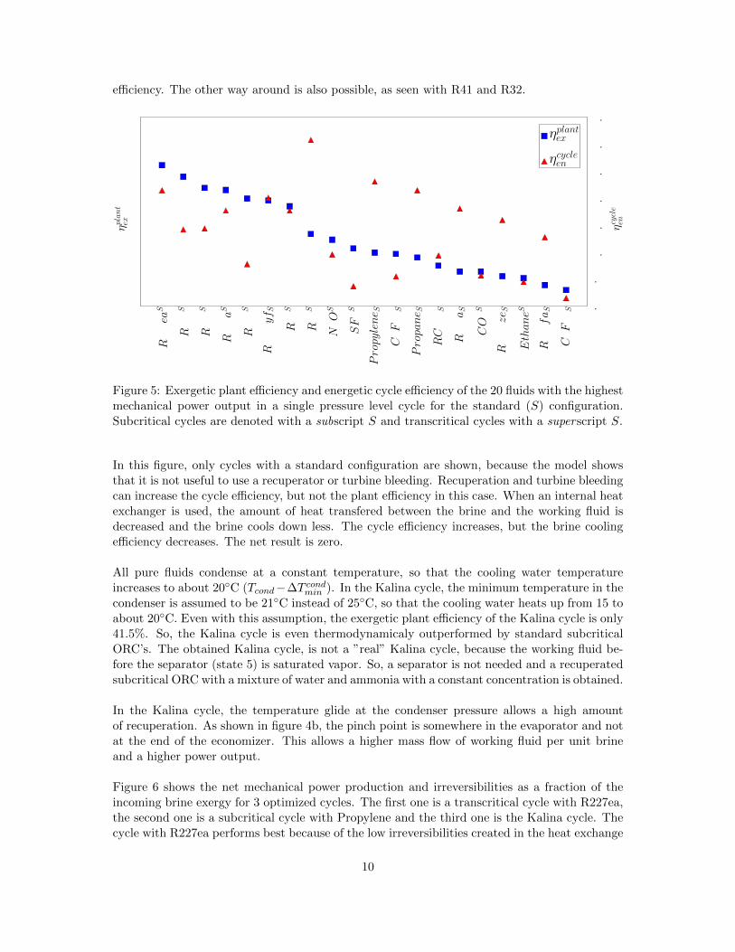
Figure 6 shows the net mechanical power production and irreversibilities as a fraction of theincoming brine exergy for 3 optimized cycles. The first one is a transcritical cycle with R227ea,the second one is a subcritical cycle with Propylene and the third one is the Kalina cycle. Thecycle with R227ea performs best because of the low irreversibilities created in the heat exchange

10

between brine and working fluid and because of the high brine cooling efficiency. The pressureratio in this cycle is high, so the irreversibilities created in the pump and turbine are high too.The combination of the high brine cooling efficiency and the average cycle efficiency causesrelatively high irreversibilities in the cooling installation.

R227ea Propylene Kalina0

20

40

60

80

100

Fra

ctio

nof

inco

min

gex

ergy

[%]

Eout

Irecup

Imix

IT

IHX

IP

Icool

Wnet

Figure 6: Net mechanical power production and irreversibilities created, as fraction of theincoming brine exergy for the optimum transcritical cycle with R227ea, the optimum subcriticalcycle with Propylene and the optimum Kalina cycle.

The subcritical cycle with Propylene performs better than the Kalina cycle because of thehigher brine cooling efficiency and the lower irreversibilities created in the high-pressure heatexchange (IHX and Irecup). In the Kalina cycle, the lower irreversibilities generated in the con-denser (temperature glide), turbine and pump cannot compensate this.

One of the advantages of the Kalina cycle would be the temperature glide. This tempera-ture glide causes a low creation of irreversibilities in the condenser, but not in the high-pressureheat exchanger. Some standard subcritical ORC’s even outperform the Kalina cycle consideredin this context. This comparison is only thermodynamical, so no economic conclusions aremade.

b Dual pressure

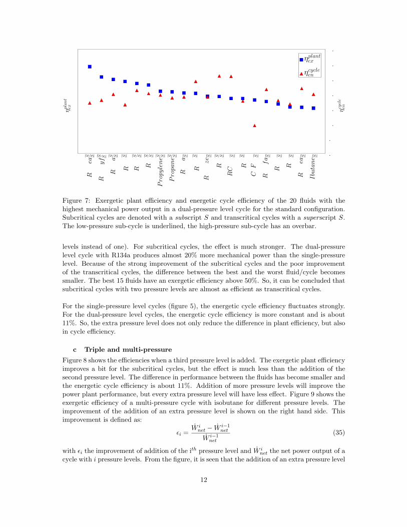
It is also possible to use more than 1 pressure level. The exergetic plant (�) and energetic cycle(4) efficiency for the 20 fluids with the highest power output in a dual-pressure level cycle areshown in figure 7. Again, only the standard configuration is shown because of the same reasonas before.

The cycles with the highest mechanical power output are almost all a combination of a subcrit-ical cycle with a transcritical one, but the addition of the subcritical part does not improve theplant efficiency very much (e.g. for R227ea an increase of 3% is obtained by using 2 pressure

11

R22

7eaS S

R12

34yfS S

R14

3aS S

R11

5S

R12

5S S

R32

S S

PropyleneS S

PropaneS S

R13

4aS

R21

8S

R12

34ze

S

R22

S S

RC

318 S

R41

S

C4F

10S

R23

6faS

R12

4 S

R12

S

R23

6eaS

Ibutane S

40

45

50

55

60

ηplant

ex[%

]ηplantex

ηcycleen

9.0

9.5

10.0

10.5

11.0

11.5

12.0

12.5

ηcycle

en[%

]

Figure 7: Exergetic plant efficiency and energetic cycle efficiency of the 20 fluids with thehighest mechanical power output in a dual-pressure level cycle for the standard configuration.Subcritical cycles are denoted with a subscript S and transcritical cycles with a superscript S.The low-pressure sub-cycle is underlined, the high-pressure sub-cycle has an overbar.

levels instead of one). For subcritical cycles, the effect is much stronger. The dual-pressurelevel cycle with R134a produces almost 20% more mechanical power than the single-pressurelevel. Because of the strong improvement of the subcritical cycles and the poor improvementof the transcritical cycles, the difference between the best and the worst fluid/cycle becomessmaller. The best 15 fluids have an exergetic efficiency above 50%. So, it can be concluded thatsubcritical cycles with two pressure levels are almost as efficient as transcritical cycles.

For the single-pressure level cycles (figure 5), the energetic cycle efficiency fluctuates strongly.For the dual-pressure level cycles, the energetic cycle efficiency is more constant and is about11%. So, the extra pressure level does not only reduce the difference in plant efficiency, but alsoin cycle efficiency.

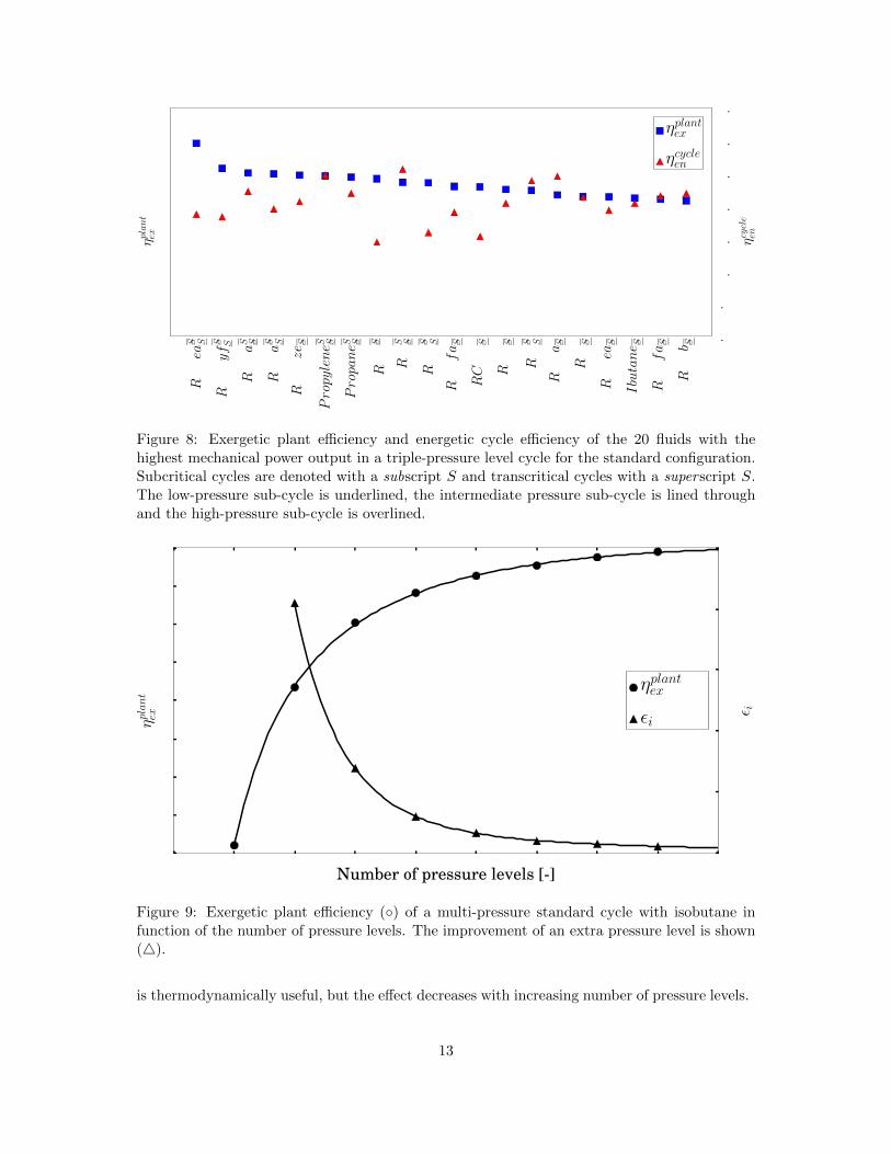
c Triple and multi-pressure

Figure 8 shows the efficiencies when a third pressure level is added. The exergetic plant efficiencyimproves a bit for the subcritical cycles, but the effect is much less than the addition of thesecond pressure level. The difference in performance between the fluids has become smaller andthe energetic cycle efficiency is about 11%. Addition of more pressure levels will improve thepower plant performance, but every extra pressure level will have less effect. Figure 9 shows theexergetic efficiency of a multi-pressure cycle with isobutane for different pressure levels. Theimprovement of the addition of an extra pressure level is shown on the right hand side. Thisimprovement is defined as:

εi =W i

net − W i−1net

W i−1net

(35)

with εi the improvement of addition of the ith pressure level and W inet the net power output of a

cycle with i pressure levels. From the figure, it is seen that the addition of an extra pressure level

12

R22

7eaS− S

R12

34yfS− S

R13

4aS S−

R14

3aS− S

R12

34ze

S−

PropyleneS S−

PropaneS S−

R11

5S−

R22

S S−

R12

5S− SR

236faS−

RC

318 S−

R12

4 S−

R32

S− SR

152a

S−

R12

S−

R23

6eaS−

Ibutane S−

R24

5faS−

R14

2bS−40

45

50

55

60

ηplant

ex[%

]ηplantex

ηcycleen

9.0

9.5

10.0

10.5

11.0

11.5

12.0

12.5

ηcycle

en[%

]

Figure 8: Exergetic plant efficiency and energetic cycle efficiency of the 20 fluids with thehighest mechanical power output in a triple-pressure level cycle for the standard configuration.Subcritical cycles are denoted with a subscript S and transcritical cycles with a superscript S.The low-pressure sub-cycle is underlined, the intermediate pressure sub-cycle is lined throughand the high-pressure sub-cycle is overlined.

0 1 2 3 4 5 6 7 8 9Number of pressure levels [-]

40

42

44

46

48

50

52

54

56

ηplant

ex[%

]

ηplantex [%]

εi[%]

0

5

10

15

20

25

ε i[%

]

Figure 9: Exergetic plant efficiency (◦) of a multi-pressure standard cycle with isobutane infunction of the number of pressure levels. The improvement of an extra pressure level is shown(4).

is thermodynamically useful, but the effect decreases with increasing number of pressure levels.

13

1 pressure 2 pressure 3 pressure0

20

40

60

80

100

Fra

ctio

nof

inco

min

gex

ergy

[%]

Eout

Irecup

IT

IHX

IP

Icool

Wnet

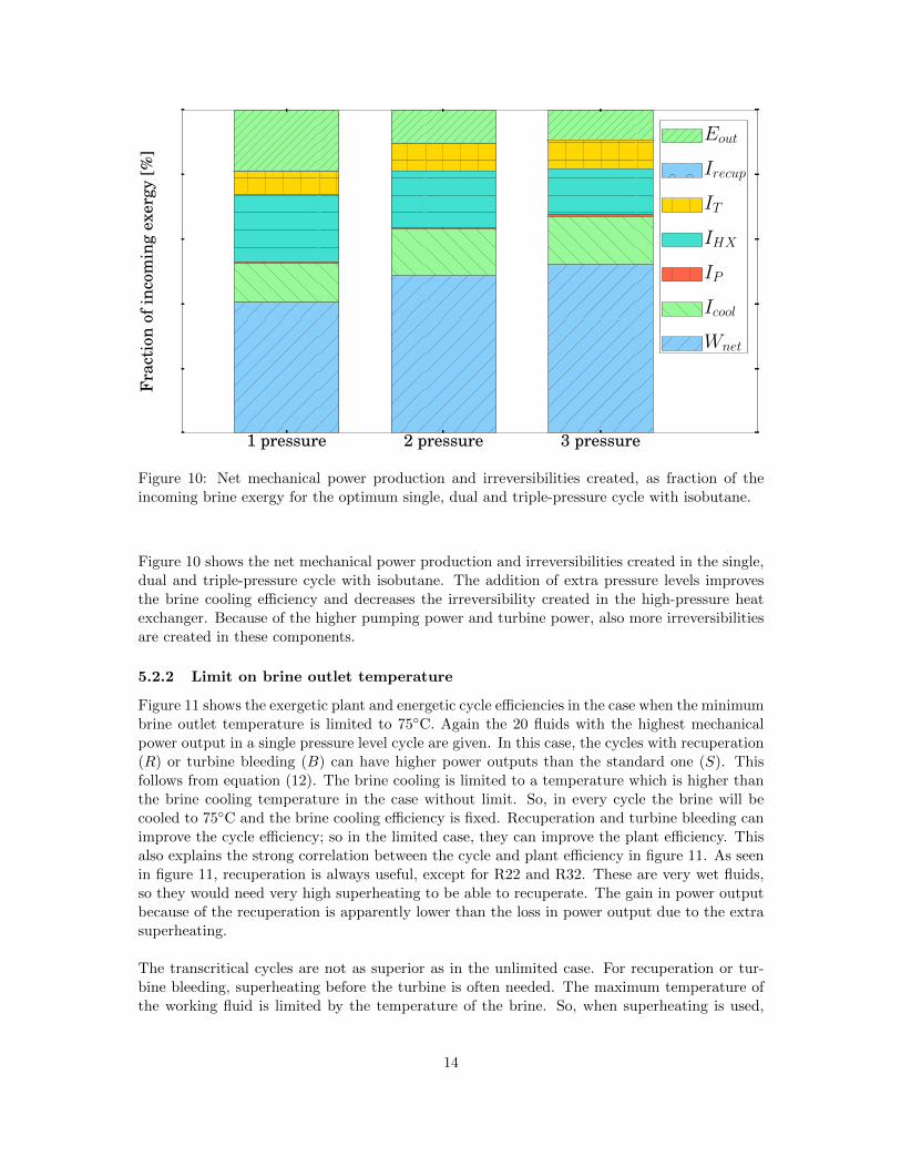
Figure 10: Net mechanical power production and irreversibilities created, as fraction of theincoming brine exergy for the optimum single, dual and triple-pressure cycle with isobutane.

Figure 10 shows the net mechanical power production and irreversibilities created in the single,dual and triple-pressure cycle with isobutane. The addition of extra pressure levels improvesthe brine cooling efficiency and decreases the irreversibility created in the high-pressure heatexchanger. Because of the higher pumping power and turbine power, also more irreversibilitiesare created in these components.

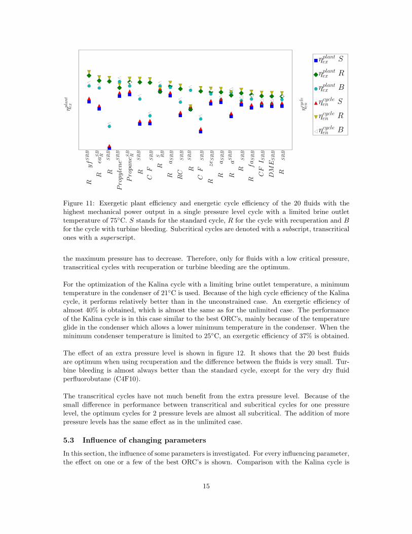
5.2.2 Limit on brine outlet temperature

Figure 11 shows the exergetic plant and energetic cycle efficiencies in the case when the minimumbrine outlet temperature is limited to 75◦C. Again the 20 fluids with the highest mechanicalpower output in a single pressure level cycle are given. In this case, the cycles with recuperation(R) or turbine bleeding (B) can have higher power outputs than the standard one (S). Thisfollows from equation (12). The brine cooling is limited to a temperature which is higher thanthe brine cooling temperature in the case without limit. So, in every cycle the brine will becooled to 75◦C and the brine cooling efficiency is fixed. Recuperation and turbine bleeding canimprove the cycle efficiency; so in the limited case, they can improve the plant efficiency. Thisalso explains the strong correlation between the cycle and plant efficiency in figure 11. As seenin figure 11, recuperation is always useful, except for R22 and R32. These are very wet fluids,so they would need very high superheating to be able to recuperate. The gain in power outputbecause of the recuperation is apparently lower than the loss in power output due to the extrasuperheating.

The transcritical cycles are not as superior as in the unlimited case. For recuperation or tur-bine bleeding, superheating before the turbine is often needed. The maximum temperature ofthe working fluid is limited by the temperature of the brine. So, when superheating is used,

14

R12

34yfSRB

R22

7eaSB

R

R21

8SRB

PropyleneS

RB

PropaneS

BR

R11

5SRB

C4F

10SRB

R22

S RB

R13

4aSRB

RC

318 S

RB

R32

SRB

C5F

12SRB

R12

34ze

SRB

R15

2aSRB

R14

3aSRB

R12

SRB

R23

6faSRB

CF

3ISRB

DMESRB

R12

4 SRB30

32

34

36

38

40

42

44

ηplant

ex[%

]ηplantex (S)

ηplantex (R)

ηplantex (B)

ηcycleen (S)

ηcycleen (R)

ηcycleen (B)

10

11

12

13

14

15

ηcycle

en[%

]

Figure 11: Exergetic plant efficiency and energetic cycle efficiency of the 20 fluids with thehighest mechanical power output in a single pressure level cycle with a limited brine outlettemperature of 75◦C. S stands for the standard cycle, R for the cycle with recuperation and Bfor the cycle with turbine bleeding. Subcritical cycles are denoted with a subscript, transcriticalones with a superscript.

the maximum pressure has to decrease. Therefore, only for fluids with a low critical pressure,transcritical cycles with recuperation or turbine bleeding are the optimum.

For the optimization of the Kalina cycle with a limiting brine outlet temperature, a minimumtemperature in the condenser of 21◦C is used. Because of the high cycle efficiency of the Kalinacycle, it performs relatively better than in the unconstrained case. An exergetic efficiency ofalmost 40% is obtained, which is almost the same as for the unlimited case. The performanceof the Kalina cycle is in this case similar to the best ORC’s, mainly because of the temperatureglide in the condenser which allows a lower minimum temperature in the condenser. When theminimum condenser temperature is limited to 25◦C, an exergetic efficiency of 37% is obtained.

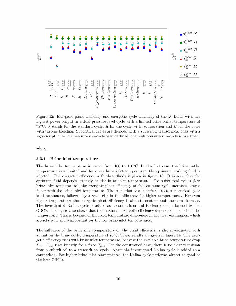
The effect of an extra pressure level is shown in figure 12. It shows that the 20 best fluidsare optimum when using recuperation and the difference between the fluids is very small. Tur-bine bleeding is almost always better than the standard cycle, except for the very dry fluidperfluorobutane (C4F10).

The transcritical cycles have not much benefit from the extra pressure level. Because of thesmall difference in performance between transcritical and subcritical cycles for one pressurelevel, the optimum cycles for 2 pressure levels are almost all subcritical. The addition of morepressure levels has the same effect as in the unlimited case.

5.3 Influence of changing parameters

In this section, the influence of some parameters is investigated. For every influencing parameter,the effect on one or a few of the best ORC’s is shown. Comparison with the Kalina cycle is

15

R22

7eaSRB

RB

C4F

10SRB

R24

5faSRB

R24

5caSRB

R23

6eaSRB

R23

6faSRB

Butane S

RB

RC

318 S

RB

Cyclohexane S

RB

Ibutane S

RB

Pentane S

RB

Trans-butene S

RB

R12

4 SRB

Ibutene S

RB

Ipentane S

RB

Butene S

RB

R11

3 SRB

R11

4 SRB

Cis

-butene S

RB

R12

34ze

S SRB30

32

34

36

38

40

42

44

ηplant

ex[%

]ηplantex (S)

ηplantex (R)

ηplantex (B)

ηcycleen (S)

ηcycleen (R)

ηcycleen (B)10

11

12

13

14

15

ηcycle

en[%

]

Figure 12: Exergetic plant efficiency and energetic cycle efficiency of the 20 fluids with thehighest power output in a dual pressure level cycle with a limited brine outlet temperature of75◦C. S stands for the standard cycle, R for the cycle with recuperation and B for the cyclewith turbine bleeding. Subcritical cycles are denoted with a subscript, transcritical ones with asuperscript. The low pressure sub-cycle is underlined, the high pressure sub-cycle is overlined.

added.

5.3.1 Brine inlet temperature

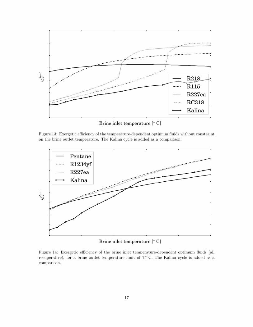
The brine inlet temperature is varied from 100 to 150◦C. In the first case, the brine outlettemperature is unlimited and for every brine inlet temperature, the optimum working fluid isselected. The exergetic efficiency with these fluids is given in figure 13. It is seen that theoptimum fluid depends strongly on the brine inlet temperature. For subcritical cycles (lowbrine inlet temperature), the exergetic plant efficiency of the optimum cycle increases almostlinear with the brine inlet temperature. The transition of a subcritical to a transcritical cycleis discontinuous, followed by a weak rise in the efficiency for higher temperatures. For evenhigher temperatures the exergetic plant efficiency is almost constant and starts to decrease.The investigated Kalina cycle is added as a comparison and is clearly outperformed by theORC’s. The figure also shows that the maximum exergetic efficiency depends on the brine inlettemperature. This is because of the fixed temperature differences in the heat exchangers, whichare relatively more important for the low brine inlet temperatures.

The influence of the brine inlet temperature on the plant efficiency is also investigated witha limit on the brine outlet temperature of 75◦C. These results are given in figure 14. The exer-getic efficiency rises with brine inlet temperature, because the available brine temperature dropTin − Tout rises linearly for a fixed Tout. For the constrained case, there is no clear transitionfrom a subcritical to a transcritical cycle. Again the investigated Kalina cycle is added as acomparison. For higher brine inlet temperatures, the Kalina cycle performs almost as good asthe best ORC’s.

16

100 110 120 130 140 150Brine inlet temperature [◦ C]

30

35

40

45

50

55

60

65

ηplant

ex[%

]

R218R115R227eaRC318Kalina

Figure 13: Exergetic efficiency of the temperature-dependent optimum fluids without constrainton the brine outlet temperature. The Kalina cycle is added as a comparison.

100 110 120 130 140 150Brine inlet temperature [◦ C]

15

20

25

30

35

40

45

50

55

ηplant

ex[%

]

PentaneR1234yfR227eaKalina

Figure 14: Exergetic efficiency of the brine inlet temperature-dependent optimum fluids (allrecuperative), for a brine outlet temperature limit of 75◦C. The Kalina cycle is added as acomparison.

17

5.3.2 Limit on brine temperature

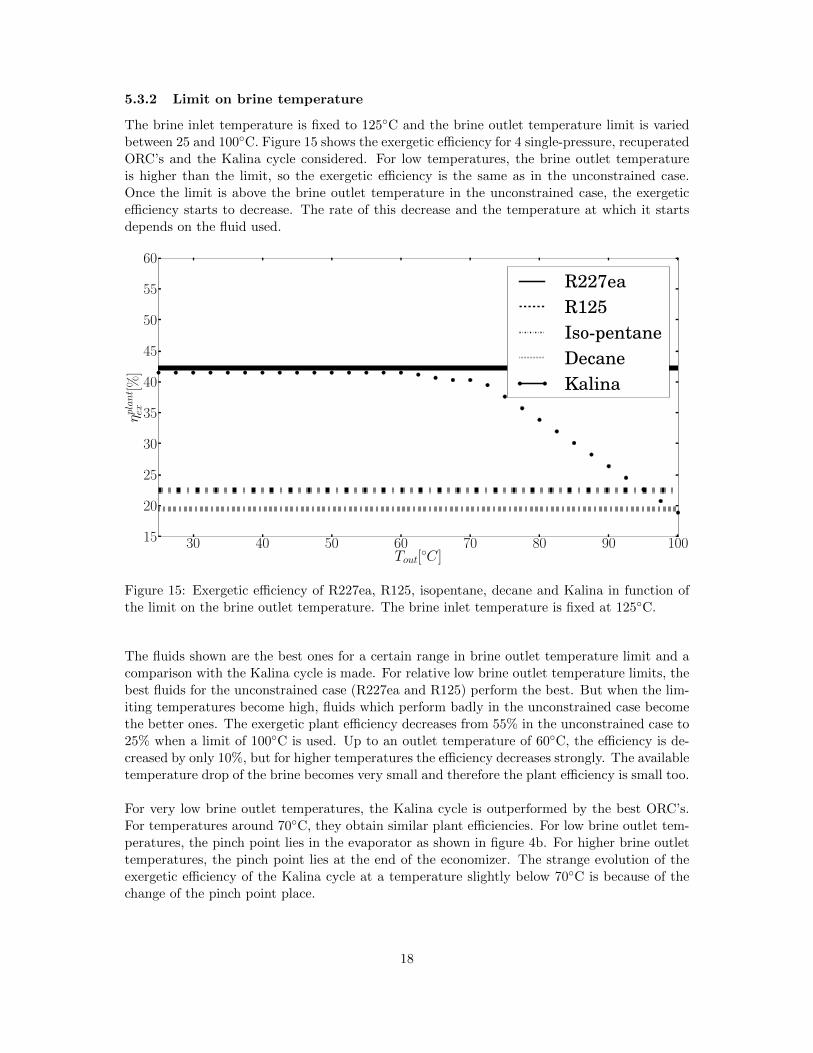
The brine inlet temperature is fixed to 125◦C and the brine outlet temperature limit is variedbetween 25 and 100◦C. Figure 15 shows the exergetic efficiency for 4 single-pressure, recuperatedORC’s and the Kalina cycle considered. For low temperatures, the brine outlet temperatureis higher than the limit, so the exergetic efficiency is the same as in the unconstrained case.Once the limit is above the brine outlet temperature in the unconstrained case, the exergeticefficiency starts to decrease. The rate of this decrease and the temperature at which it startsdepends on the fluid used.

Figure 15: Exergetic efficiency of R227ea, R125, isopentane, decane and Kalina in function ofthe limit on the brine outlet temperature. The brine inlet temperature is fixed at 125◦C.

The fluids shown are the best ones for a certain range in brine outlet temperature limit and acomparison with the Kalina cycle is made. For relative low brine outlet temperature limits, thebest fluids for the unconstrained case (R227ea and R125) perform the best. But when the lim-iting temperatures become high, fluids which perform badly in the unconstrained case becomethe better ones. The exergetic plant efficiency decreases from 55% in the unconstrained case to25% when a limit of 100◦C is used. Up to an outlet temperature of 60◦C, the efficiency is de-creased by only 10%, but for higher temperatures the efficiency decreases strongly. The availabletemperature drop of the brine becomes very small and therefore the plant efficiency is small too.

For very low brine outlet temperatures, the Kalina cycle is outperformed by the best ORC’s.For temperatures around 70◦C, they obtain similar plant efficiencies. For low brine outlet tem-peratures, the pinch point lies in the evaporator as shown in figure 4b. For higher brine outlettemperatures, the pinch point lies at the end of the economizer. The strange evolution of theexergetic efficiency of the Kalina cycle at a temperature slightly below 70◦C is because of thechange of the pinch point place.

18

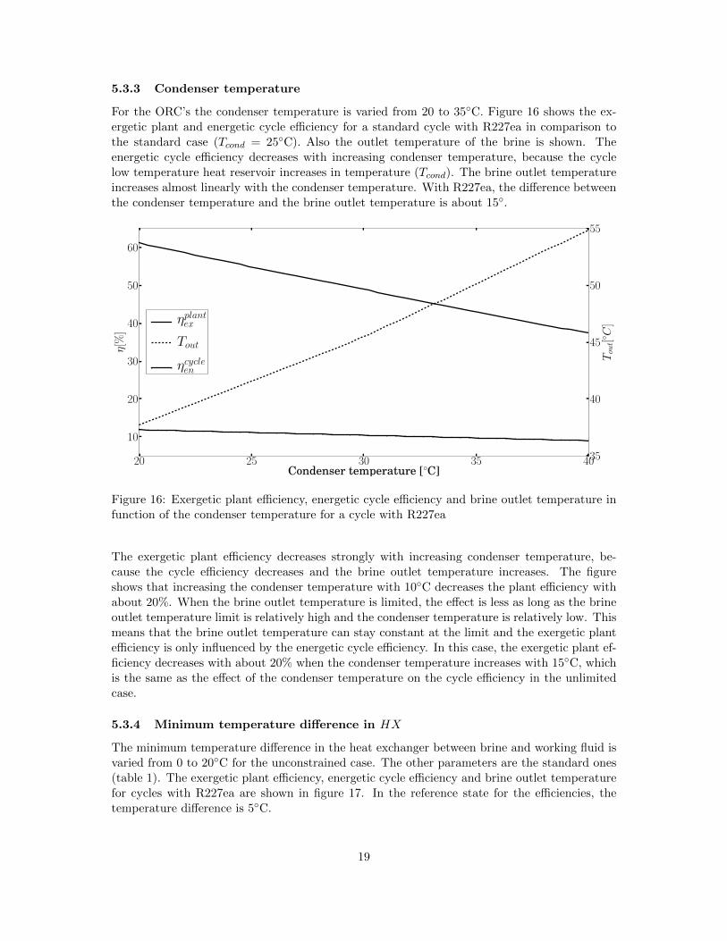
5.3.3 Condenser temperature

For the ORC’s the condenser temperature is varied from 20 to 35◦C. Figure 16 shows the ex-ergetic plant and energetic cycle efficiency for a standard cycle with R227ea in comparison tothe standard case (Tcond = 25◦C). Also the outlet temperature of the brine is shown. Theenergetic cycle efficiency decreases with increasing condenser temperature, because the cyclelow temperature heat reservoir increases in temperature (Tcond). The brine outlet temperatureincreases almost linearly with the condenser temperature. With R227ea, the difference betweenthe condenser temperature and the brine outlet temperature is about 15◦.

Figure 16: Exergetic plant efficiency, energetic cycle efficiency and brine outlet temperature infunction of the condenser temperature for a cycle with R227ea

The exergetic plant efficiency decreases strongly with increasing condenser temperature, be-cause the cycle efficiency decreases and the brine outlet temperature increases. The figureshows that increasing the condenser temperature with 10◦C decreases the plant efficiency withabout 20%. When the brine outlet temperature is limited, the effect is less as long as the brineoutlet temperature limit is relatively high and the condenser temperature is relatively low. Thismeans that the brine outlet temperature can stay constant at the limit and the exergetic plantefficiency is only influenced by the energetic cycle efficiency. In this case, the exergetic plant ef-ficiency decreases with about 20% when the condenser temperature increases with 15◦C, whichis the same as the effect of the condenser temperature on the cycle efficiency in the unlimitedcase.

5.3.4 Minimum temperature difference in HX

The minimum temperature difference in the heat exchanger between brine and working fluid isvaried from 0 to 20◦C for the unconstrained case. The other parameters are the standard ones(table 1). The exergetic plant efficiency, energetic cycle efficiency and brine outlet temperaturefor cycles with R227ea are shown in figure 17. In the reference state for the efficiencies, thetemperature difference is 5◦C.

19

0 5 10 15 20Temperature difference in HX [◦C]

50

60

70

80

90

100

110

120

η/η

0[%

] ηplantex /ηplantex,0

ηcycleen /ηcycleen,0

Tout

30

35

40

45

50

55

60

65

70

Tout[◦ C

]

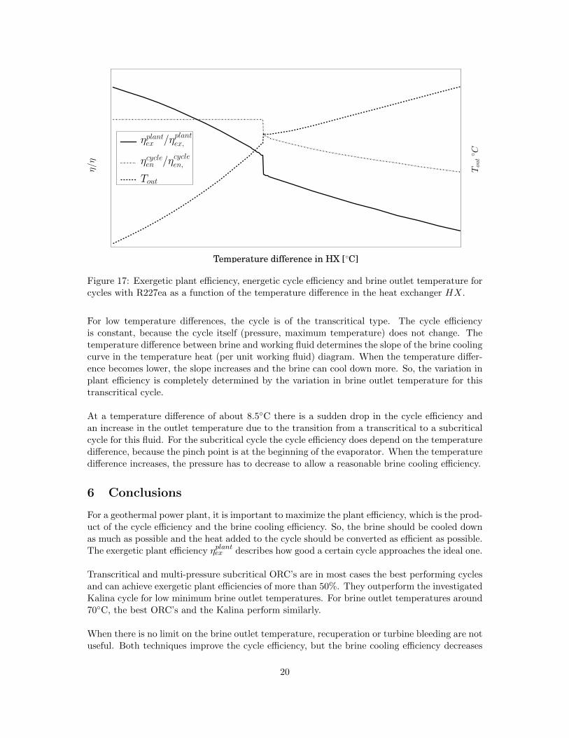
Figure 17: Exergetic plant efficiency, energetic cycle efficiency and brine outlet temperature forcycles with R227ea as a function of the temperature difference in the heat exchanger HX.

For low temperature differences, the cycle is of the transcritical type. The cycle efficiencyis constant, because the cycle itself (pressure, maximum temperature) does not change. Thetemperature difference between brine and working fluid determines the slope of the brine coolingcurve in the temperature heat (per unit working fluid) diagram. When the temperature differ-ence becomes lower, the slope increases and the brine can cool down more. So, the variation inplant efficiency is completely determined by the variation in brine outlet temperature for thistranscritical cycle.

At a temperature difference of about 8.5◦C there is a sudden drop in the cycle efficiency andan increase in the outlet temperature due to the transition from a transcritical to a subcriticalcycle for this fluid. For the subcritical cycle the cycle efficiency does depend on the temperaturedifference, because the pinch point is at the beginning of the evaporator. When the temperaturedifference increases, the pressure has to decrease to allow a reasonable brine cooling efficiency.

6 Conclusions

For a geothermal power plant, it is important to maximize the plant efficiency, which is the prod-uct of the cycle efficiency and the brine cooling efficiency. So, the brine should be cooled downas much as possible and the heat added to the cycle should be converted as efficient as possible.The exergetic plant efficiency ηplantex describes how good a certain cycle approaches the ideal one.

Transcritical and multi-pressure subcritical ORC’s are in most cases the best performing cyclesand can achieve exergetic plant efficiencies of more than 50%. They outperform the investigatedKalina cycle for low minimum brine outlet temperatures. For brine outlet temperatures around70◦C, the best ORC’s and the Kalina perform similarly.

When there is no limit on the brine outlet temperature, recuperation or turbine bleeding are notuseful. Both techniques improve the cycle efficiency, but the brine cooling efficiency decreases

20

and the combination of these two effects has zero influence on the plant efficiency. A limit onthe brine outlet temperature causes a strong decrease in the power plant output, but in thiscase the decrease can partly be compensated by the use of recuperation or turbine bleeding.The Kalina cycle performs relatively better when the brine outlet temperature is limited.

The maximum theoretical temperature drop of the brine is low, because of the low brine inlettemperature. A small increase in the condenser temperature or the pinch point temperaturedifference, have a relatively strong influence on the available temperature drop of the brine andtherefore also on the plant efficiency. So, for low temperature heat sources, it is very importantto have a low condenser temperature and pinch point temperature difference.

Acknowledgments

Daniel Walraven is supported by a VITO doctoral grant.

References

[1] J.W. Tester, B. Anderson, A. Batchelor, D. Blackwell, R. DiPippo, E. Drake, J. Garnish, B. Livesay,M.C. Moore, and K. Nichols. The Future of Geothermal Energy: Impact of Enhanced GeothermalSystems (EGS) on the United States in the 21st Century. Technical report, Massachusetts Instituteof Technology, Massachusetts, USA, 2006.

[2] H. Paschen, D. Oertel, and R. Grunwald. Moglichkeiten geothermischer Stromerzeugung in Deutsch-land. TAB Arbeitsbericht Nr. 84, 2003.

[3] A. Schuster, S. Karellas, E. Kakaras, and H. Spliethoff. Energetic and economic investigation oforganic rankine cycle applications. Applied thermal engineering, 29(8-9):1809–1817, 2009.

[4] E. Cayer, N. Galanis, and H. Nesreddine. Parametric study and optimization of a transcriticalpower cycle using a low temperature source. Applied Energy, 87(4):1349–1357, 2010.

[5] M. Kanoglu. Exergy analysis of a dual-level binary geothermal power plant. Geothermics, 31(6):709–724, 2002.

[6] Z. Gnutek and A. Bryszewska-Mazurek. The thermodynamic analysis of multicycle orc engine.Energy, 26(12):1075–1082, 2001.

[7] F. Heberle and D. Bruggemann. Exergy based fluid selection for a geothermal organic rankine cyclefor combined heat and power generation. Applied Thermal Engineering, 30(11-12):1326–1332, 2010.

[8] P.J. Mago, L.M. Chamra, K. Srinivasan, and C. Somayaji. An examination of regenerative organicrankine cycles using dry fluids. Applied thermal engineering, 28(8-9):998–1007, 2008.

[9] M. Yari. Exergetic analysis of various types of geothermal power plants. Renewable Energy, 35(1):112–121, 2010.

[10] B. Saleh, G. Koglbauer, M. Wendland, and J. Fischer. Working fluids for low-temperature organicrankine cycles. Energy, 32(7):1210–1221, 2007.

[11] H.A. Mlcak. An Introduction to the Kalina Cycle. Proceedings of the International Joint PowerGeneration Conference, 30:1–11, 1996.

[12] S. Ogriseck. Integration of Kalina cycle in a combined heat and power plant, a case study. AppliedThermal Engineering, 29(14-15):2843–2848, 2009.

[13] P. Valdimarsson. Factors influencing the economics of the Kalina power cycle and situations ofsuperior performance. Manager, pages 32–40, 2003.

21

[14] R. DiPippo. Second Law assessment of binary plants generating power from low-temperaturegeothermal fluids. Geothermics, 33(5):565–586, 2004.

[15] E.W. Lemmon, M.L. Huber, and M.O. Mclinden. NIST Reference Fluid Thermodynamic and Trans-port Properties REFPROP. The National Institute of Standards and Technology (NIST), 2007.Version 8.0.

22