Comparison of the e ﬃciency of translation operators used ...

Comparison of the efficiency of translation operators used in thefast multipole method for the 3D Laplace equation

Nail A. Gumerov and Ramani Duraiswami

April 12, 2005

Abstract

We examine the practical implementation of a fast multipole method algorithm for therapid summation of Laplace multipoles. Several translation operators with different asymptoticcomputational and memory complexities have been proposed for this problem. These algorithmsinclude: Method 0 — the originally proposed matrix based translations due to Greengard andRokhlin (1987), Method 1 — the rotation, axial translation and rotation algorithm due to Whiteand Martin Head-Gordon (1993), and Method 3 — the plane-wave version of the multipole-to-local translation operator due to Greengard and Rokhlin (1997). We compare the algorithmson data sets of varying size and with varying imposed accuracy requirements. While from theliterature it would have been expected that method 2 would always be the method of choice, atleast as far as computational speed is concerned, we find that this is not always the case. Wefind that as far as speed is concerned the choice between methods 1 and 2 depends on problemsize and error requirements. Method 2 is the algorithm of choice for large problems where highaccuracy is required, though the advantage is not clear cut, especially if memory requirementsare an issue. If memory is an issue, Method 1 is the method of choice for most problems. Anew analysis of the computational complexities of the algorithms is provided, which explainsthe observed results. We provide guidelines for choosing parameters for FMM algorithms.

1 Introduction

Many problems in electrostatics, fluid mechanics, molecular dynamics, stellar dynamics, etc., canbe reduced to evaluation of the field due to a large number of monopole or multipole sources locatedat locations xα, α = 1 . . . , N.. For such problems, usually, the most expensive computational partis related to performing a matrix-vector multiplication or summation of the type

v (yj) =NXi=1

uiΦ (yj − xi) , j = 1, ...,M (1)

where Φ (y − x) is some function (e.g., the Green’s function or multipole solution for the Laplaceequation) centered at x, which must be evaluated at locations yj . Here ui are some coefficients(e.g. the intensities of the monopole or multipole sources). Straightforward computation of thesesums, which also can be considered to be the multiplication of a M × N matrix with elementsΦji = Φ (yj − xi) by a N vector with components ui to obtain a M vector with componentsvj = v (yj) , obviously requires O (MN) operations. The point sets yj and xi in these problemsmay be different, or the same. If the points yj and xi coincide, the evaluation of Φ must beappropriately regularized (e.g., in a boundary element application, quadrature over the elementwill regularize the function). In the sequel we assume that this issue, if it arises, is dealt with.

1

Gumerov & Duraiswami, 2005 University of Maryland, CS TR 4701, UMIACS TR-2005-09

The Fast Multipole Method, introduced by Greengard and Rokhlin [Greengard87], seeks tospeed up the matrix-vector product by performing it approximately, but with a guaranteed specifiedaccuracy. The main idea in the FMM is to split the sum into a near and a far field

v (yj) =X

xi∈RnearuiΦ (yj − xi) +

Xxi∈Rfar

uiΦ (yj − xi) , (2)

and build factored approximate representations of the functions Φ in the far-field

Φ (yj − xi) =P−1Xl=0

Sl (yj − x∗)Rl (xi − x∗) +O (²) , (3)

which usually come from analytical series representations, and are truncated at some number ofcoefficients P, which is a function of the desired precision ² (= ² (P )). These factorizations areusually in terms of a singular set of multipole solutions Sl, and a regular set of solutions Rl. Thesefactored parts allow one to separate the computations involving the points sets xi and yj , andconsolidate operations for many points.

Xxi∈Rfar

uiΦ (yj − xi) =X

xi∈Rfarui

P−1Xl=0

Sl (yj − x∗)Rl (xi − x∗) (4)

=P−1Xl=0

Sl (yj − x∗)X

xi∈RfaruiRl (xi − x∗) =

P−1Xl=0

ClSl (yj − x∗) (5)

The coefficients Cl for all xi are built and then used in the evaluation at all yj . This reduces thecost of this part of the summation to linear order, and reduces the memory requirements to thisorder as well.

No global factorization (that is quickly convergent) is available, and the split between the nearand far-fields must be managed on a part by part basis. This is done by using appropriate datastructures, and a variety of representations are used. Due to the dependence of the error on thenumber of points, the cost of building data-structures that allow this factor, effectively the algorithmachieves a complexity of O(M logM +N logN),which can be substantially faster than the directproduct for large M and N.

Thus, the FMM is an approximate method, and a feature of its analysis and implementation isthe evaluation of the errors. One should not be misled into thinking that the FMM is not accurate.If desired, even machine precision can be achieved, making the solution indistinguishable from an“exact” algorithm. Since its introduction in the late 1980s, the fast multipole method (FMM)has been hailed as one of the top ten algorithms of the 20th century. FMM inspired algorithmshave appeared for the solution of various problems of both matrices associated with the Laplacepotential, and with those of other equations (the biharmonic, Helmholtz, Maxwell) and in unrelatedareas (for general radial basis functions).

When one wishes to implement an FMM algorithm from the material presented in the literature,one is faced with several choices, and the situations where each of these choices should be the correctone is not clear. The purpose of this paper is to describe these choices for the potentials of theLaplace equation, and then present the results of the tests on algorithms implemented with thesechoices, in terms of their accuracy, their speed of computation, the memory required, and theirease of implementation. Analysis that helps explain the results is also provided.

2


1.1 Scope of this paper

The issues we consider in this paper areTranslation operators: In the FMM we build various representations of the functions (these

will be described below). To convert from one representation in a particular coordinate frame, to thesame, or different, representation centered in another coordinate frame, one must “translate” therepresentation. A typical representation involves p2 coefficients. In the original FMM [Greengard87]the translation operators were p2× p2 matrices, that acted on the coefficients of one representationto provide the coefficients in the other, at a cost of O(p4) operations per translation. White andHead-Gordon [White96] provided translation operators that used symmetries in the representingfunctions along certain the axial coordinate directions, to achieve the translation via a sequenceof rotation, translation and rotation operations, which require O(p3) operations per translation.Greengard and Rokhlin [Greengard97] presented a method that reduced the cost of the most costlyof the translation operations to O

¡p2¢,though the process of converting the functions to this

representation remained at O(p3), and the other translations follow the O(p3) or O(p4) translationmethod. This method also requires more memory resources than for the other translation operators.

Desired accuracy: Often the FMM is used in a certain context, where there are certain errorsinherent in the remaining numerical procedures (e.g., in representation of surfaces or boundaries,in the values of experimentally measured data, etc.) and the FMM should be accurate enough thatit does not worsen the error in the computation, but should not unnecessarily expend resources inseeking to achieve accuracy that is more than necessary. Corresponding to each desired accuracy,the translation methods will have different values of p. A systematic comparison of the values ofp (and as a consequence the desired error ²) at which each of these translation methods is mosteffective, has to our knowledge not been presented (the original papers just compare the resultswith the direct matrix-vector product). This paper attempts to fill this lacuna in the literature.

Memory resources: One of the FMM’s big promises arises due to its requirement of orderof magnitude smaller memory. This should allow simulations to be effectively run on the desktopcomputers of scientists. As such in many applications the memory requirements may be the de-termining factor in the choice of an algorithm. We accordingly compare the use of the memory inFMM algorithms with varying problem size, error requirements, and memory budgets. An inter-esting aspect of our experience was that for many problems, larger memory leads to larger time onthe commodity architectures we considered.

1.2 Other fast algorithms not considered

One can find several other O(N) or O(N logN) methods for solution of problem (1), that are notconsidered here mainly because they either do not appear efficient enough, or cannot achieve thenecessary accuracy. We briefly discuss these methods, and why we do not consider them.

The first of these are “tree-code” methods due to Barnes and Hut [Barnes86]. This algorithmwas introduced a year or so earlier than the FMM and currently is used in astrophysics [Dehnen02]and other areas e.g., vortex dynamics, [Lindsay01]. In its current version, this method shows highperformance for relatively low accuracy simulations, and in fact may be the most efficient methodfor some problems. The speed of the method relative to the FMM reduces as higher accuracy isrequired. This is related to the need to use smaller “opening angles” - the parameter, which controlsseparation of the group of points. We did some preliminary tests, which show that for low accuracythe Barnes and Hut method with some improvements can indeed perform better than the FMM,as has been reported by Dehnen [Dehnen02]. However, for the higher accuracy (beyond 10−5) it ismuch slower than the FMM.

3


Another class of methods are the global FFT-based methods (e.g. FFTM, [Ong04]). These donot employ hierarchical data structures, and while there can be savings related to data structuresbecause of this, some disadvantages are also obvious. One of them is related to the adaptivity.The regular FMM skips “empty” boxes, while more advanced adaptive versions (e.g. [Cheng99],[Gumerov2005]) provide substantial savings for non-uniform data. Another disadvantage is relatedto the use of O(p4) multipole-to-local translation operators in the FFTM (p2 is the number ofterms in the multipole expansion), which results in a total O(p4N logN) complexity. While theperformance of the FFTM relative to the FMM should be more carefully analyzed in terms ofthe asymptotic constants, we note that the FMM-based algorithms of complexity O(p3N) or evenO(Np2 log p) are available. Further, even from the viewpoint of memory utilization, these methodsrequire more memory. Thus, while interesting and somewhat simpler to code, the method appearsnot competitive.

Finally, we mention some translation approaches which appear to have superior asymptoticcomplexity for p → ∞, of (O(p2 log p)), but in practice do not appear competitive. Elliott andBoard [Elliott02] proposed to use the 2D Toeplitz-Hankel structure of the translation matrices, tospeed-up multiplication with them using the FFT. They reported speedups 2 and 4 for a sequentialand 3 and 6 for a vector processor for p = 8 and p = 16, respectively, compared to the originalO(p4) method. This shows that while formally the method is scaled as O(p2 log p) the asymptoticconstant of the method is larger than one, and, in fact, speedups for the sequential processorare even smaller than when using the above-mentioned O(Np3) method, which for p = 8 and 16provides 8/3 > 2 and 16/3 > 4 speedups. The same situation relates to algorithms exploitingdecompositions of translation operators to 1D structured matrices [Tang03], which despite lower(O(p2 log p)) asymptotic complexity have larger asymptotic constants. In practice, p is normallybelow 25 even for high accuracy computations, and these methods are slower than the O(Np3)methods in practice.

1.3 Organization of the paper

We describe the fast multipole method using the various translation operators in Section 2. Theseinclude the matrix-based translation (Method #0), the rotation axial-translation and rotationmethod (Method #1) and the plane-wave translation (Method #2). In Section 3 we provide somedetails of the FMM algorithm. Section 4 describes the numerical tests performed to determine theproblems for which each type of algorithm may be useful. Finally section 5 provides a discussionand conclusions. Using these results one can choose the algorithm appropriate to the problem athand.

2 Translation theory

2.1 Multipole and local expansions

Elementary solutions of the Laplace equation in three dimensions in spherical coordinates (r, θ,ϕ)

x = r sin θ cosϕ, x = r sin θ sinϕ, z = r cos θ, (6)

can be represented as

Rmn (r) = αmn rnY mn (θ,ϕ), Smn (r) = βmn r

−n−1Y mn (θ,ϕ), n = 0, 1, ..., m = −n, ..., n. (7)

Here Rmn (r) are respectively the regular (local) and Smn (r) the singular (far field, or multipole)

spherical basis functions, αmn and βmn are normalization constants selected by convenience, and

4


Y mn (θ,ϕ) are the orthonormal spherical harmonics:

Y mn (θ,ϕ) = Nmn P

|m|n (µ)eimϕ, µ = cos θ, (8)

Nmn = (−1)m

s2n+ 1

4π

(n− |m|)!(n+ |m|)! , n = 0, 1, 2, ..., m = −n, ..., n,

where P |m|n (µ) are the associated Legendre functions [Abramowitz65]. We will use the definitionof the associated Legendre function Pmn (µ) that is consistent with the value on the cut (−1, 1) ofthe hypergeometric function Pmn (z) (see Abramowitz & Stegun, [Abramowitz65]). These functionscan be obtained from the Legendre polynomials Pn (µ) via the Rodrigues’ formula

Pmn (µ) = (−1)m¡1− µ2

¢m/2 dmdµm

Pn (µ) , Pn (µ) =1

2nn!

dn

dµn¡µ2 − 1

¢n. (9)

Our definition of spherical harmonics coincides with that of Epton & Dembart [Epton95], except fora factor

p(2n+ 1)/4π, which we include to make them an orthonormal basis over the sphere. In

[Cheng99] the factor (−1)m in Nmn in Eq. (8) is omitted in what seems to be a typographical error,

since further translation and conversion formulae sometimes are valid for harmonics containing thisfactor.

The Green’s function for the Laplace equation can be written in the form

G(r, r0) =1

4π |r− r0|=

∞Xn=0

nXm=−n

R−mn (r0)Smn (r)

α−mn βmn (2n+ 1), |r0| < |r| . (10)

An arbitrary harmonic function regular inside a sphere can be expanded inside this sphere into alocal expansion

φ (r) =∞Xn=0

nXm=−n

φmn Rmn (r) . (11)

Also an arbitrary harmonic function that decays at the infinity and is regular outside a sphere canbe expanded outside this sphere as a multipole expansion

φ (r) =∞Xn=0

nXm=−n

φmn Smn (r) . (12)

The coefficients φmn in (11) and (12) are the expansion coefficients.Consider now a p-truncated approximation of φ (r) in the form

φ (r) =

p−1Xn=0

nXm=−n

φmn Fmn (r) , F = S,R. (13)

This approximation is characterized by p2 expansion coefficients φmn which can be stacked in asingle vector, which we call the “representing” vector. For a general complex function the lengthof representation is p2 complex numbers, or 2p2 real numbers. If φ (r) is real, then we have, e.g.for the regular expansion

φ (r) =

p−1Xn=0

nXm=−n

φmn Rmn (r) =

p−1Xn=0

nXm=−n

φmn αmn r

nY mn (θ,ϕ) (14)

=

p−1Xn=0

nXm=−n

φmn αmn r

nY −mn (θ,ϕ) =

p−1Xn=0

nXm=−n

φ−mn α−mn rnY mn (θ,ϕ) =

p−1Xn=0

nXm=−n

φ−mnα−mnαmn

Rmn (r) .

5


Comparing this with expansion (13) and due to the completeness of the spherical harmonic basiswe have the following symmetry

φ−mn α−mn = αmn φmn . (15)

So the real harmonic functions φ (r) can be represented by vectors of half the length, which storethe real and imaginary parts of coefficients φmn (e.g. if α

mn = 1 all φ

0n are real (p quantities) and all

φmn for m > 0 can be represented by p2 − p real numbers, then φ−mn do not require storage).

2.2 Translation operators

2.2.1 Reexpansions of elementary solutions

Elementary solutions of the Laplace equation centered at a point can be expanded in series overelementary solutions centered about some other spatial point. This can be written as the followingaddition theorems

Rmn (r+ t) =∞Xn0=0

n0Xm0=−n0

(R|R)m0mn0n (t)Rm

0n0 (r) , (16)

Smn (r+ t) =∞Xn0=0

n0Xm0=−n0

(S|R)m0mn0n (t)Rm

0n0 (r) , |r| < |t| ,

Smn (r+ t) =∞Xn0=0

n0Xm0=−n0

(S|S)m0mn0n (t)Sm

0n0 (r) , |r| > |t| ,

where t is the translation vector, and (R|R)m0mn0n , (S|R)m0m

n0n , and (S|S)m0mn0n are the four index local-

to-local, multipole-to-local, and multipole-to-multipole reexpansion coefficients. Explicit expres-sions for these coefficients can be found elsewhere (see e.g. [Epton95, Cheng99]).

We define the following complex normalization factors

αm(1)n = (−1)n i−|m|s

4π

(2n+ 1) (n−m)!(n+m)! , βm(1)n = i|m|r4π (n−m)!(n+m)!

2n+ 1,(17)

n = 0, 1, ...., m = −n, ..., n.If we set then αmn = αm(1)n and βmn = βm(1)n in the definitions of the basis functions (7) then thereexpansion coefficients take a particularly simple form (see [Epton95]):

(R|R)m0mn0n (t) = Rm−m

0n−n0 (t),

¯m0¯6 n0, (18)

(S|R)m0mn0n (t) = Sm−m

0n+n0 (t),

¯m0¯ 6 n0, |m| 6 n,

(S|S)m0mn0n (t) = Rm−m

0n0−n (t), |m| 6 n.

In the other commonly used case the normalization constants are selected as αmn = 1 and βmn = 1.In this case we have

(R|R)m0mn0n =

αm0

(1)n0αm−m0(1)n−n0

αm(1)nRm−m

0n−n0 (t), (19)

(S|R)m0mn0n =

αm0

(1)n0βm−m0(1)n+n0

βm(1)nSm−m

0n+n0 (t),

(S|S)m0mn0n =

βm0

(1)n0αm−m0(1)n0−n

βm(1)nRm−m

0n0−n (t),

6


where αm(1)n and βm(1)n are given by Eq. (17).

2.2.2 Translation using truncated reexpansion matrices (Method #0)

Arranging the reexpansion coefficients to form a truncated reexpansion matrices yields a straight-forward translation method (here and below we refer to this as Method #0). Let φ (r) be anarbitrary scalar function, φ : Ω (r) → C, where Ω (r) ⊂ R3. For a given vector t ∈R3 We define anew function bφ : bΩ (r) → C, bΩ (r) ⊂ R3 such that in bΩ (r) = Ω (r+ t) the values of bφ (r) coincidewith the values of φ (r+ t) and we treat bφ (r) as a result of the action of the translation operatorT (t) on φ (r):

bφ = T (t) [φ] , bφ (r) = φ (r+ t) , r ∈bΩ (r) ⊂ R3. (20)

The function can be represented by the (infinite) vector of coefficients multiplying their associatedbasis functions. If φ (r) be a regular solution of the Laplace equation inside a sphere Ωa of radiusa, that includes the origin, it can be represented in the form

φ (r) =∞Xn=0

nXm=−n

φmn Rmn (r) , (21)

where φmn are the expansion coefficients over the basis Rmn (r). Similarly a solution of Laplace’sequation φ (r) regular outside a sphere Ωa can be expanded over the basis Smn (r). The translatedfunction bφ (r) can be also be expanded over the bases Rmn (r) or Smn (r) with expansion coeffi-cients bφmn . Due to linearity of the translation operator the sets nbφmn o and φmn will be related by atranslation operator (an infinite matrix), which represents the translation operator in the respectivebases.

If bφ is expanded over the same basis as φ, Eq. (21), in Ωa ⊂ bΩ (r) ∩ Ω (r):bφ (r) = ∞X

n=0

nXm=−n

bφmn Rmn (r) . (22)

Then we have

∞Xn=0

nXm=−n

bφmn Rmn (r) = bφ (r) = φ (r+ t) =∞Xn0=0

n0Xm0=−n0

φm0

n0 Rm0n0 (r+ t) (23)

=∞Xn=0

nXm=−n

" ∞Xn0=0

n0Xm0=−n0

(R|R)mm0nn0 (t)φ

m0n0

#Rmn (r) ,

which shows that

bφmn = ∞Xn0=0

n0Xm0=−n0

(R|R)mm0nn0 (t)φ

m0n0 , (24)

assuming that all the series converge absolutely and uniformly.It is not difficult to prove that for any ² we can find some p such that¯¯bφ (r)−

p−1Xn=0

nXm=−n

bφ(p)mn Rmn (r)

¯¯ < ², bφ(p)mn =

p−1Xn0=0

n0Xm0=−n0

(R|R)mm0nn0 (t)φ

m0n0 . (25)

7


We call p the truncation number. The number of coefficients bφ(p)mn is p2 and to perform the

local-to-local translation we multiply a dense matrixn(R|R)mm0

nn0 (t)oby the input representing

vectornφm

0n0o. A straightforward multiplication by the translation operation will take O(p4) mul-

tiplications/additions, even though the coefficients (R|R)mm0nn0 can be stacked into upper triangular

matrix.Similar consideration can be given to multipole-to-local and multipole-to-multipole translation

operators, which are represented by matrices (S|R)m0mn0n (t) and (S|S)m0m

n0n (t), respectively. Fordetails we refer to [Greengard87], [Epton95], [Greengard97].

The translation matrices have Toeplitz/Hankel structure — and this fact that can be potentiallyexploited for faster matrix-vector multiplication [Elliott02] to reduce formally the procedure toO(p2 log p) operations.However the use of the fast Fourier transforms in the translation processcan be justified only at sufficiently large p due to large asymptotic constants in the O(p2 log p)complexity dependence. Normally, such values of p are not encountered in the solution of theLaplace equation, where sufficient accuracy can be achieved at smaller p.

Finally we note that in the FMM we do not translate the function, but change the centerof expansion. For example, under local-to-local translation from center r1 to center r2 we meanrepresentation of the same function in the regular bases centered at these point respectively. Sincefor representations of the same function we have

∞Xn=0

nXm=−n

φmn Rmn (r− r1) =

∞Xn=0

nXm=−n

bφmn Rmn (r− r2) , (26)

it is not difficult to see that the expansion coefficients are related by Eq. (24), where the trans-lation vector is t = r2−r1.The same relates to the multipole-to-local and multipole-to-multipoletranslations, where we use the S|R and S|S matrices instead of the R|R translation matrix. Figure1 provides illustration of the different types of translation operators used in the FMM.

r1

r2

tr1

r2

t

r2

r1

t

Local-to-Local (R|R) Multipole-to-Local (S|R) Multipole-to-Multipole (S|S)

r1

r2

tr1

r2

tr1

r2

t

r1

r2

t

r2

r1

tr2

r1

t

Local-to-Local (R|R) Multipole-to-Local (S|R) Multipole-to-Multipole (S|S)

Figure 1: Illustration of local-to-local (R|R), multipole-to-local (S|R), and multipole-to-multipole(S|S) translations from expansion center r1 to expansion center r2 (translation vector t = r2−r1).The star shows location of a source (singular point). Expansion about center r1 is valid inside thelighter and darker gray area, while expansion about center r2 is valid only in the darker gray area(subdomain of the lighter gray area). The source (sources) can be located in the white domains.

8


2.3 “Point-and-shoot” translation method (Method #1)

The “point-and-shoot” translation method (using the colorful terminology suggested by Rokhlin),which we refer as Method #1, is based on decomposition of the translation operator to the productof rotation and coaxial translation operators. This method was described first in Ref. [White96].

2.3.1 Coaxial Translations

The coaxial translation is the translation along the z-coordinate axis, i.e. this is the case whenthe translation vector t =tiz, where iz is the basis unit vector for the z-axis. The peculiarity ofthe coaxial translation is that it does not change the order m of the translated coefficients, and sotranslation can be performed for each order independently. For example, Eq. (24) for the coaxiallocal-to-local translation will be reduced to

bφmn = ∞Xn0=|m|

(R|R)mnn0 (t)φmn0 , m = 0,±1, ..., n = |m| , |m|+ 1, .... (27)

The three index coaxial reexpansion coefficients (F |E)mnn0 (F,E = S,R; m = 0,±1,±2, ..., n, n0 =|m| , |m|+1, ...) are functions of the translation distance t only and can be expressed via the generalreexpansion coefficients as

(F |E)mnn0 (t) = (F |E)mmnn0 (tiz), F,E = S,R; t > 0. (28)

Using Eq. (18) we have for normalized basis functions (7) with αmn = αm(1)n and βmn = βm(1)n:

(R|R)mnn0 (t) = rn0−n (t) , n0 > |m| , (29)

(S|R)mnn0 (t) = sn+n0(t), n, n0 > |m| ,(S|S)mnn0 (t) = rn−n0(t), n > |m| ,

where the functions rn (t) and sn (t) are

rn (t) =(−t)n

n!, sn (t) =

n!

tn+1n = 0, 1, ..., t > 0, (30)

and zero for n < 0. This show that for given m matrices (R|R)mnn0 (t) are upper triangular,(S|S)mnn0 (t) are lower triangular, and (S|R)

mnn0 (t) is a fully populated matrix. The latter

matrix is symmetric, while (S|S)mnn0 (t) = (R|R)mn0n (t), i.e. these matrices are transposes ofeach other. It is also important to note that the coaxial translation matrices are real.

It is not difficult then to write expressions for coaxial translation coefficients in the basis offunctions normalized with αmn = 1 and βmn = 1 (see Eqs. (17), (19), and (29)). In this basis allmatrices remain real, but lose the symmetry properties, mentioned above.

For p-truncated function representations by its expansion coefficients, the number of operationsrequired to perform a single coaxial translation with dense matrix (multipole-to-local) is

NCoax(p) =

p−1Xm=−(p−1)

⎛⎝ p−1Xn=|m|

1

⎞⎠2 = p−1Xm=−(p−1)

(p− |m|)2 = 1

3p¡2p2 + 1

¢. (31)

This number is obtained assuming that 1 operation is spent for multiplication/addition (assumingthat the translation matrices can be precomputed and stored). Note that this estimate is validfor real φmn . Generally, these coefficients are complex, and so for multipole-to-local translation one

9


should spent 2NCoax(p) real multiplications/additions. In case when φmn represent real functionφ (r) the count of operations goes back to NCoax(p) due to the symmetry of expansion coefficients(e.g. for functions normalized with αmn = βmn = 1 we have φ−mn = φmn and with αmn = αm(1)n,

βmn = βm(1)n symmetry φ−mn = (−1)m φmn holds). Further we will count only operations requiredfor translations of real functions, since the complex functions can be computed by independenttransforms of the real and imaginary parts (so the number of operations simply doubles).

Note that for local-to-local and multipole-to-multipole coaxial translations we have the followingestimate

N(R|R)Coax (p) = N

(S|S)Coax (p) =

p−1Xm=−(p−1)

p−1Xn=|m|

nXn0=|m|

=1

2

p−1Xm=−(p−1)

(p− |m|)(p− |m|+ 1) (32)

=1

2

£NCoax(p) + p

2¤.

This is because the corresponding matrices are upper or lower triangular.

2.3.2 Rotations

To perform translation with an arbitrary vector t using the computationally cheap coaxial trans-lation operators, we first must rotate the original reference frame to align the z-axis of the rotatedreference frame with t, translate and then perform an inverse rotation.

x

y

z

x

y

z

O

AAβ

α

x

yz

x

y

z

OA

Aβ

x

y

z

x

y

z

O

AA

x

y

z

xx

yy

zz

O

AAA

x

yz

x

y

z

OA

A

x

yz

xx

yy

zz

OA

AA

γ

x

y

z

x

y

z

O

AAβ

α

x

yz

x

y

z

OA

Aβ

x

y

z

x

y

z

O

AA

x

y

z

xx

yy

zz

O

AAA

x

yz

x

y

z

OA

A

x

yz

xx

yy

zz

OA

AA

γ

Figure 2: The figure on the left shows the transformed axes (x, y, z) in the original reference frame(x, y, z) . The spherical polar coordinates of the point A lying on the z axis on the unit sphere are(β,α) . The figure on the right shows the original axes (x, y, z) in the transformed reference frame(x, y, z) . The coordinates of the point A lying on the z axis on the unit sphere are (β, γ) . Thepoints O, A, and A are the same in both figures. All rotation matrices can be derived in terms ofthese three angles α, β, γ.

An arbitrary rotation in three dimensions can be characterized by three Euler angles, or anglesα,β, and γ that are simply related to them. For the forward rotation, when (θ,ϕ) are the spherical

10


polar angles of the rotated z-axis in the original reference frame, then β = θ, α = ϕ; for the inverserotation with

³bθ, bϕ´ the spherical polar angles of the original z-axis in the rotated reference frame,β = bθ, γ = bϕ (see Fig. 2). An important property of the spherical harmonics is that on rotationtheir degree n does not change, i.e.

Y mn (θ,ϕ) =nX

m0=−nTm

0mn (α,β, γ)Y m

0n

³bθ, bϕ´ , n = 0, 1, 2, ..., m = −n, ..., n, (33)

where (θ,ϕ) and³bθ, bϕ´ are spherical polar angles of the same point on the unit sphere in the

original and the rotated reference frames, and Tm0m

n (α,β, γ) are the rotation coefficients.Rotation transform for solution of the Laplace equation factorized over the regular spherical

basis functions can be performed as.

φ (r) =∞Xn=0

nXm=−n

φmn Rmn (r) =

∞Xn=0

rnnX

m=−nφmn α

mn Y

mn (θ,ϕ) (34)

=∞Xn=0

nXm0=−n

"nX

m=−nTm

0mn (α,β, γ)αmn φ

mn

#rnY m

0n

³bθ, bϕ´ = ∞Xn=0

nXm=−n

bφmn Rmn (br) ,where r and br are coordinates of the same field point in the original and rotated frames, while φmnand bφmn are the respective expansion coefficients related as

bφmn = nXm0=−n

Tmm0

n (α,β, γ)αm0

n

αmnφm

0n . (35)

The same holds for the multipole expansions where in Eq. (35) one should replace αmn andαm

0n normalization constants with βmn and βm

0n , respectively. In case αmn = βmn the rotation co-

efficients for the regular and singular basis functions are the same.Rotation coefficients Tm

0mn (α,β, γ) can be decomposed as

Tm0m

n (α,β, γ) = eimαe−im0γHm0m

n (β) , (36)

wherenHm0mn (β)

ois a dense real symmetric matrix. Its entries can be computed using an analytical

expression, or by a fast recursive procedure (see [Gumerov2005]), which starts with the initial value

Hm00n (β) = (−1)m0

s(n− |m0|)!(n+ |m0|)!P

|m0|n (cosβ), n = 0, 1, ..., m0 = −n, ..., n, (37)

and further propagates for positive m:

Hm0,m+1n−1 =

1

bmn

½1

2

hb−m

0−1n (1− cosβ)Hm0+1,m

n − bm0−1n (1 + cosβ)Hm0−1,m

n

i− am0

n−1 sinβHm0mn

¾,

(38)

n = 2, 3, ..., m0 = −n+ 1, ..., n− 1, m = 0, ..., n− 2,where amn = b

mn = 0 for n < |m| , and

amn = a−mn =

s(n+ 1 +m)(n+ 1−m)

(2n+ 1) (2n+ 3), for n > |m| , (39)

bmn =

⎧⎨⎩q(n−m−1)(n−m)(2n−1)(2n+1) , 06m6n,

−q

(n−m−1)(n−m)(2n−1)(2n+1) , −n6 m <0.

.

11


For negative m coefficients Hm0mn (β) can be found using symmetry H−m

0,−mn (β) = Hm0m

n (β).

We note that inverse rotation can be performed using the matrixn¡T−1

¢m0mn

(α,β, γ)o, which

is the complex conjugate transposed ofnTm

0mn (α,β, γ)

oand can be simplified using Eq. (36):

¡T−1

¢m0mn

(α,β, γ) = Tmm0n (α,β, γ) = e−im

0αeimγHmm0n (β) = e−im

0αeimγHm0mn (β) = Tm

0mn (γ,β,α) .

(40)

In the “point-and-shoot” method the angle γ can be selected arbitrarily, since the direction of thetranslation vector t is characterized only by the two angles, α and β. For example, one could simplyset γ = 0. We found however, that setting γ = α can be computationally cheaper, since in this casethe forward and inverse translation operators coincide,

n¡T−1

¢m0mn

(α,β,α)o=nTm

0mn (α,β,α)

o(for the normalization αmn = βmn = 1).

In any case, the entries of the rotation matrix can be precomputed and stored. The number ofoperations required for one rotation of vector of size p2 then can be counted as

NRot(p) =

p−1Xn=0

ÃnX

m=−n1

!2=

p−1Xn=0

(2n+ 1)2 =1

3p¡4p2 − 1

¢. (41)

As before we assumed here that one operation is required for multiplication/addition (precomputedrotation matrices). This is true for rotation of coefficients of real functions, due to the abovementioned symmetry, and this number should be multiplied by 2 for general complex coefficients.In the latter case we note that decomposition (36) with γ = 0 can be more efficient, since complexmultiplications should be performed only for diagonal matrix with entries eimα (O(p2) operations)

while dense matrix multiplication involves real matrixnHm0mn (β)

o.

The operation count (31) and (41) brings the total complexity of the multipole-to-local trans-lation of coefficients of real functions for the Method #1 to

N(S|R)1 (p) = NRot(p) +Ncoax(p) +NRot(p) =

1

3p¡2p2 + 1

¢+2

3p¡4p2 − 1

¢≈ 103p3. (42)

Comparing this with the complexity of the same operation using straightforward multiplication ofa dense matrix (Method #0), which we refer as

N(S|R)0 (p) = p4, (43)

we can see that for p > 4 Method #1 should be theoretically faster than Method #0.We also note that for local-to-local and multipole-to-multipole translations, the number of

operations using Method #1 can be evaluated as (see Eq. (32)):

N(S|S)1 (p) = NRot(p) +N

(S|S)coax (p) +NRot(p) =

1

6p¡2p2 + 1

¢+1

2p2 +

2

3p¡4p2 − 1

¢≈ 3p3. (44)

2.4 Exponential expansions

One of the most expensive operation in the FMM is the multipole-to-local translation. Whilethe cost of a single S|R-translation operation is comparable with the cost of the R|R- and S|S-operations, the number of multipole-to-local translations is much larger (approximately hundredtimes). To reduce the cost of this operation Greengard and Rokhlin [Greengard97] (see also Cheng et

12


al. [Cheng99]) proposed to use the exponential expansions (also referred as “plane wave” expansionsin analogy with similar expansions introduced for the wave equation; physically, this is not correct,since the Laplace equation is an elliptic equation). The plane wave expansions are based on thefollowing representation of the Green’s function (10) in the domain z > z0:

G(r, r0) =1

8π2

Z ∞

0e−λ(z−z0)

Z 2π

0eiλ[(x−x0) cosα+(y−y0) sinα]dαdλ, (45)

r = (x, y, z) , r0 = (x0, y0, z0), z > z0.

In Refs. [Greengard97, Cheng99] the following quadrature for the integrals is proposed when

a 6 z − z0 6 b,q(x− x0)2 + (y − y0)2 6 c, (46)

where a, b and c are some numbers (for the 3-D FMMwith the standard 1-neighborhoods [Gumerov2003],the approximation should be valid for a = 1, b = 4, c = 4

√2):

G(r, r0) =1

4π

S(²)Xk=1

wkMk

e−λk(z−z0)MkXj=1

eiλk[(x−x0) cosαjk+(y−y0) sinαjk], (47)

where λk and αjk = 2πj/Mk (j = 1, ...,Mk) are the quadrature nodes, wk are the weights, Mk isthe number of nodes in the kth subspace where the discrete Fourier transform with respect to αis performed, and S(²) is some number dependent on the accuracy of approximation, ². As thisnumber varies the quadrature nodes and weights as well as Mk vary also. For particular cases withS (²) = 8, 17, 26, which we refer as the order of quadrature, the nodes and weights can be found inRefs. [Greengard97, Cheng99].

This quadrature generates a more general representation valid not only for the Green function,but for an arbitrary multipole expansion of the Laplace equation, that can be viewed as a sum ofsources located inside some domain. So if a harmonic function φ (r) is regular in Ω and has allsingularities inside Ω0, such that and for any r0 ∈ Ω0 and r ∈ Ω condition (46) holds, then φ (r)can approximated in Ω with the specified accuracy ² with the following expansion:

φ (r) =

S(²)Xk=1

MkXj=1

Wkje−λkzeiλk(x cosαjk+y sinαjk), (48)

where Wkj are the expansion coefficients.The exponential expansion, therefore, provides an alternative to the spherical multipole and

local expansions, and is generated by expansion of a harmonic function in cylindrical coordinates(in a bounded cylindrical domain). The length of a representation using this expansion is

Sexp =

S(²)Xk=1

Mk (49)

complex numbers or 2Sexp real numbers. This can be reduced by half for real functions due to thesymmetry

Wkj =Wk,j+Mk/2, j = 1, ...,Mk/2. (50)

Indeed, we have

αj+Mk/2,k =2π (j +Mk/2)

Mk= π + αjk, j = 1, ...,Mk/2. (51)

13


So

eiλk(x cosαj+Mk/2,k+y sinαj+Mk/2,k

) = e−iλk(x cosαjk+y sinαjk) = eiλk(x cosαjk+y sinαjk), (52)

and comparing expansions (48) for φ (r) and φ (r), that should be the same, we obtain Eq. (50).Finally we note that S(²) and Sexp are related to the truncation number p, which provides the

same error ² as

S(²) = κp, Sexp = σp2, (53)

where κ and σ are some constants, which can be found from numerical tests.

2.5 Exponential translation and conversion (Method #2)

The exponential expansion diagonalizes the translation operator, since the exponents are its eigen-functions. Based on Eq. (49) we have

φ (r+ t) =

S(²)Xk=1

MkXj=1

Wkje−λktzeiλk(tx cosαjk+ty sinαjk)e−λkzeiλk(x cosαjk+y sinαjk) (54)

=

S(²)Xk=1

MkXj=1

cWkje−λkzeiλk(x cosαjk+y sinαjk) = bφ (r) ,

where cWkj are the coefficients of the translated function bφ (r) :cWkj = EkjWkj , Ekj = e

−λktzeiλk(tx cosαjk+ty sinαjk), t = (tx, ty, tz). (55)

If the exponential translation coefficients Ekj are precomputed and stored, then translation re-quires N exp

rep complex-by-complex multiplications for translation of a complex function and Nexprep

complex-by-real multiplications for translation of real function. So the number of real multiplica-tion operations for translation of coefficients of real function is

N (E|E)(Sexp) = 2Sexp = 2σp2, (56)

and double this for the complex case.In the version of the FMM in [Greengard97, Cheng99] the exponential translation is applied

only to reduce the cost of the multipole-to-local translations, while multipole-to-multipole, andlocal-to-local translations are performed with a traditional scheme. This method, therefore, alsorequires multipole-to-exponential and exponential-to-local conversions.

Note that Eq. (54) is given in the form that follows from Eq. (48). Since the FMM employsa hierarchical data structure with different size boxes at different levels, the nodes and weights ofthe quadrature should be scaled to appropriate box size d. Namely, the nodes λk and weights wkin the quadrature should be replaced by λk/d and wk/d as λk and wk are obtained for a unit box(indeed multiplication of r by d reduces the value of the Green function d times). According tothe [Greengard97, Cheng99] and our normalization of the spherical harmonics the multipole-to-exponential, or S|E, transform can be performed as

Wkj =wkMkd

p−1Xm=−(p−1)

eimαjk

p−1Xn=|m|

1

βmn βm(1)n

µλkd

¶nφmn , k = 1, .., s(²), j = 1, ...,Mk, (57)

14


where βm(1)n is provided by Eq. (17) and βmn is an arbitrary normalization factor for the singularbasis functions (7).

Being thought of as a linear operation with matrix of sizeN exprep ×p2 the above conversion requires

O¡N exprep p2

¢operation. However, Eq. (57) provides a subspace decomposition of the conversion

operation (similar to coaxial translation), since first the inner sum can be computed for all m andk and then the outer sum can be computed for all k and j. For precomputed and stored coefficientscomputation of the inner sum requires s (²) (p− |m|) operations for the mth subspace and all k.Note that if coefficients βmn selected to be equal βm(1)n then coefficients in the inner sum are real

(if βmn = 1 factor i|m| from βm(1)n can be taken out of the inner summation). This means that the

number of real multiplication for all subspaces (taking into account the symmetry of φmn for realfunctions) is

N(S|E)(inner) = S (²)

p−1Xm=−(p−1)

(p− |m|) = S (²)p−1X

m=−(p−1)(p− |m|) = S (²) p2. (58)

Computation of the outer sum requires then Mk complex multiplications per each element(m, k). This results in the following count of real multiplications:

N(S|E)(outer) = Sexp

p−1Xm=−(p−1)

2 = 2 (2p− 1)Sexp. (59)

This count includes symmetry of the expansion coefficient (50). Therefore, the actual complexityof the (S|E) operation is

N (S|E) = N (S|E)(inner) +N

(S|E)(outer) = S (²) p

2 + 2 (2p− 1)Sexp ≈ (κ+ 4σ) p3. (60)

Note that this number is referred in [Cheng99] as O(p3).The second conversion operation is conversion of the exponential expansion to local expansion,

or E|R operation. This can be performed using the following formula (we make some correctionsto what appear to be typographical errors in [Cheng99] and use our definition of the sphericalharmonics):

φmn = αmn αm(1)n

S(²)Xk=1

µλkd

¶n MkXj=1

Wkje−imαjk , (61)

where αm(1)n is provided by Eq. (17) and αmn is an arbitrary normalization constant for the regularbasis functions (7). It is not difficult to see that the operation count for the E|R conversion is exactlythe same as for the S|E conversion (k inverse discrete Fourier transforms instead of the forwardones, and one multiplication by real matrix for the mth subspace). So we have for representationsof real functions the number of real multiplications

N (E|R) = N (S|E) = S (²) p2 + 2 (2p− 1)Sexp ≈ (κ+ 4σ) p3. (62)

The advantage of the exponential expansions is that algorithmically expensive conversion op-erations can be performed far fewer times than the translation. Details of this can be found in[Cheng99] (see also the next section) and we refer the translation method using the exponentialexpansions as Method #2.

15


3 Algorithms

We will not present details of the basic FMM algorithm, which are well described in the originalpapers of Greengard, Rokhlin, and others [Greengard87], [Greengard88]. We describe some flowcharts and particulars of our implementation. The basic algorithm can be designed for low memoryconsumption (e.g. see [Gumerov2003]), though such an approach is substantially slower than thealgorithm storing data structures and using precomputed translation data, that was used in thecurrent test.

The algorithm consists of two main parts: the preset step, which includes setting the datastructure (building and storage of the neighbor lists, etc.) and precomputation and storage of alltranslation data. The data structure is generated using the bit interleaving technique describedin [Gumerov2003], which enables spatial ordering, sorting, and bookmarking. The algorithm isdesigned for two independent data sets (N arbitrary located sources and M arbitrary evaluationpoints), while for the current tests we usually used the same source and evaluation sets of length N ,which is also called the problem size. For a problem size N, the cost of building the data structurebased on spatial ordering is O(N logN), where the asymptotic constant is much smaller than theconstants in the O(N) asymptotics of the main algorithm. The number of levels could be arbitrarilyset by the user or found automatically based on the clustering parameter (the maximum numberof sources in the smallest box) for optimization of computations of problems of different size.

For efficient storage and retrieval of translation data we introduced a translation index, whichshows the direction of the translations (8 indices for each level for the S|S and R|R translationsand 343 indices for the S|R translations for each level). For the use of Method #2, which requiresalso specification of the 6 directions of the “plane wave” propagation, we also build 6 plane waveindices, which depend simply on the S|R translation indices. The translation index and the levelof space subdivision therefore uniquely specify pointers to the arrays of the translation data. Thetranslation indices for each box are stored along with the data on the boxes in the neighborhoodswhich interact with the given box. Any single translation procedure then consists in retrieval ofthe translation index, which are passed along with the representing vector (the of coefficients to betranslated) and current level to the subroutine that performs translation (say matrix-vector mul-tiplication) and returns the translated data. This scheme allows the theoretical minimum of thenumber of multiplications to be achieved but needs the algorithm to pay the price of translationdata management. We found that instead of storage of all translation data it maybe computa-tionally cheaper to manage a smaller number of translation parameters (say just the precomputedcomplex exponents eiα1k instead of the full matrix eimαjk = eimjα1k) and introduce one additionalmultiplication in the loop. If such cases were found, we used the option that results in fastestoperation. In any case our translation implementation avoids costly computation of functions likecomplex exponents and uses a small amount of multiplications in the inner loop, which we tried toreduce as much as possible.

3.1 Algorithm for Method#0 and Method#1

Figure 3 shows main steps of the standard FMM, assuming that the preset part is performedinitially. This scheme can be applied for translations using Methods #0 and #1. Here Steps 1 and2 constitute the upward pass in the box hierarchy, Steps 3,4, and 5 form the downward pass andSteps 6 and 7 relate to final summation. The upward pass is performed for boxes in the sourcehierarchy, while the downward pass and final summation are performed for the evaluation hierarchy.By “near neighborhood” we mean the box itself and its immediate neighbors, which consists of 27boxes for a box not adjacent to the boundary, and the “far neighbors”, are boxes from the parent

16


near neighborhood (of the size of the given box), which do not belong to the close neighborhood.The number of such boxes is 189 in case the box is sufficiently separated from the boundary of thedomain.

1. Get S-expansion coefficients(directly)

2. Get S-expansion coefficients from children

(S|S translation)

Level lmax

3. Get R-expansion coefficients from far neighbors

(S|R translation)

Level 2


(S|R translation)

6. Evaluate R-expansions (directly)

7. Sum sourcesin close neighborhood

(directly)

Start

End

Level lmaxLevel lmax

5. Get R-expansion coefficients from parents

(R|R translation)

Levels lmax-1,…, 2 Levels 3,…,lmax



(S|S translation)

Level lmax


(S|R translation)

Level 2


(S|R translation)

6. Evaluate R-expansions (directly)


(directly)

Start

End



(R|R translation)

Levels lmax-1,…, 2 Levels 3,…,lmax

Figure 3: A flow chart of the standard FMM (Method #0 and Method #1).

To evaluate the complexity of the algorithm we consider “the worst” case, when the sourcesand evaluation points are distributed uniformly in a cubic domain and their number is the same,N =M . Each box at the finest level contains s sources, so we have

N

s= 8lmax (63)

boxes at the finest level of space subdivision, lmax.Further we will not count the costs for expansionconsolidation operations and assume that the generation of the p2 basis functions for factorizationof the Green function (10) is Bp2, and the cost of Step 1 is Cost(1) = BNp2. The same estimateholds for Step 6, where the local expansions need to be evaluated at N points.

The cost of the multipole-to-multipole and local-to-local translations in the above methods arethe same, since both can be performed using upper triangular and transposed lower triangularmatrices. If the cost of a single S|S-translation is N (S|S), then the cost of Step 2 is

Cost(2) = N(S|S)

³8lmax + 8lmax−1 + ...+ 83

´≈ 8lmaxN (S|S). (64)

where we assume that lmax > 3 (otherwise there are no steps 4 and 5 in the algorithm). The costof Step 3 and 4 can be combined and bounded by

Cost(3+4) . 189N (S|R)³8lmax + 8lmax−1 + ...+ 83 + 82

´≈ 189 · 8lmaxN (S|R) (65)

operations, where N (S|R) is the cost of single S|R translation.Finally the cost of direct summation, or Step 7, is Cost7 ≈ 27s28lmax , since for each box at the

finest level 27s sources contribute to s evaluation points. Here we assume that one operation isspent for direct evaluation (we note that in practice a square root evaluation costs more than amultiplication).

Taking into account Eq. (63) and the above estimates, the total cost of the standard FMMexcluding the preset step is:

Cost = 2BNp2 +N

s

³2N (S|S) + 189N (S|R)

´+ 27Ns. (66)

17


This shows that the clustering parameter s heavily influences the complexity of the method. Theoptimum can be easily found by differentiating the above function with respect to s. This yieldsan optimum value of s

sopt =

∙1

27

³2N (S|S) + 189N (S|R)

´¸1/2≈³7N (S|R)

´1/2. (67)

Note that this does not depend on N . We also note that for the optimum s the costs of the thirdand the second terms in Eq. (66) are balanced. So

Cost(opt) = 2BNp2 + 54Nsopt ≈ 2BNp2 + 54N28−l(opt)max , l(opt)max = log8

N

sopt. (68)

Neglecting 2N (S|S) compared with 189N (S|R) in Eq. (66), we obtain

Cost(opt) = 2BNp2 + 54Nsopt ≈∙2Bp2 + 54

³7N (S|R)

´1/2¸N. (69)

We can substitute then N (S|R) given by Eqs. (42) and (43) to obtain theoretical estimates for thetotal cost of the FMM for Method #0 and #1:

Cost(opt)0 ≈

∙2Bp2 + 54

³7N

(S|R)0

´1/2¸N ≈ (2B + 143)Np2, (70)

Cost(opt)1 ≈

∙2Bp2 + 54

³7N

(S|R)1

´1/2¸N ≈

³2B + 261p−1/2

´Np2. (71)

This shows that both methods at large p are scaled as O(Np2), while the asymptotic constant forMethod #0 is substantially smaller (if 2B ¿ 143, which is true).

Note also that the absolute error, ², of the p-truncated approximation decays exponentially withp, which means that to guarantee that the total absolute error, ²tot = N², is bounded with growingN, p must increase as O(logN). This shows that the above methods in terms of absolute erroraccuracy scale as O(N log2N) with N . However, if a weaker error norm is sufficient for solutionof a particular problem (such as a relative L2-norm error, see the next section for a more extendeddiscussion), the the methods scale as O(N).We also note that for p1/2 ¿ 130/B (which for Laplace’sequation is the practically encountered value of p) Method#1 with optimum parameters scales asO(Np3/2), while Method #0 always scales as O(Np2).

3.2 Algorithm for Method#2

Figure 4 shows the main steps of the FMM with Method#2, assuming that the preset part isperformed. Here Steps 1,2,5,6, and 7 are the same as in Fig. 3, while Steps 3 and 4 involvingthe multipole-to-local translation are different. To provide faster S|R translation for each levell = 2, ..., lmax a loop with respect to each direction of the exponential expansion is performed. Thisis characterized by the “Plane wave index”.

Within this loop, first, we make a pass over all source boxes to convert multipole expansionsto the exponential representations (Step 3.1). The conversion for directions other than ±z requiresrotating the reference frame to point the rotated z axis towards the direction of translation, sothat the centers of the boxes being translated to lie in the region z > 2d in the rotated referenceframe. The rotation transform adds to the conversion cost (60) for the ±x and ±y directions. Note

18



(S|S translation)

Level lmax-1,…, 2Level lmax

3.1 Convert S-expansionsto E-expansions (S|E conversion)

Level 2

3.2 Get E-expansion coefficients from far neighbors

(E|E translation)

3.3. Convert E-expansions to R-expansions (E|R conversion)

4.1. Convert S-expansionsto E-expansion (S|E conversion)


(directly)

Start

End6. Evaluate R-expansions

(directly)


Level 2


(E|E translation)

Level 2

Plane wave index = 1,…,6


(R|R translation)


Plane wave index = 1,…,6Level 3,…,lmax



(S|S translation)

Level lmax-1,…, 2Level lmax

3.1 Convert S-expansionsto E-expansions (S|E conversion)

Level 2


(E|E translation)


4.1. Convert S-expansionsto E-expansion (S|E conversion)


(directly)

Start

End6. Evaluate R-expansions

(directly)


Level 2


(E|E translation)

Level 2

Plane wave index = 1,…,6


(R|R translation)


Plane wave index = 1,…,6Level 3,…,lmax


Figure 4: A flow chart of the FMM with translation performed by Method #2.

that once a transform is performed to say the x direction, the transform in the opposite direction(−x) is computationally cheap, since the multipole expansion coefficients for the same function incoordinates (x, y, z) and (bx, by, bz) = (−x, y,−z) are related asbCmn = (−1)nC−mn , (72)

(with the normalization αmn = βmn = 1). Such a transform corresponds to the change of angles(θ,ϕ)→ (π − θ,π − ϕ) , and it is not difficult to get a generalization of this equation for arbitraryαmn and βmn using the definitions (6)-(9).

By the way, this shows that it is sufficient to perform only two O(p3) real matrixnHmm0n (π/2)

orotations for axis flipping. For representations of real functions the cost per box is 2NRot(p) (asopposed to 4NRot(p) reported in the original paper [Cheng99]; however this improvement usuallyis small due to the much larger asymptotic constants for conversion of the expansions). SinceSteps 3.1 and 4.1 must be performed for each box at corresponding levels and conversion of themultipole to the exponential expansion needs to be performed for each of the 6 translation directions(±x,±y,±z) we evaluate the cost of these steps as

Cost(3.1+4.1) = (2NRot + 6N(S|E))

³8lmax + 8lmax−1 + ...+ 83 + 82

´(73)

≈ 8lmax(2NRot + 6N(S|E)) ≈ 8lmax

µ6κ+ 24σ +

8

3

¶p3,

where NRot(p) and N (S|E) are evaluated according Eqs. (41) and (60). The combined cost of Step3.3 and 4.3 is the same, due to N (S|E) = N (E|R) (see Eq. (62)) and 2 rotations are needed to flipthe axes back. The combined cost of Step 3.2 and 3.3 is given by Eq. (65), where instead of N (S|R)

we need to use N (E|E) from Eq. (56), which is valid for the real case. We obtain the total cost ofthe FMM for Method #2, where the S|S and the R|R translations are performed by Method #1(which is faster than Method #0 for p > 4),

Cost = 2BNp2 +N

s

h2N (S|S) + 2(2NRot + 6N (S|E)) + 189N (E|E)

i+ 27Ns. (74)

19


The same evaluation step cost is taken as for the other methods. Here we do not neglect the O(p2)cost of the E|E translations compared to the other terms, since the asymptotic constant 189 islarge.

This yields the optimum value of s

sopt =

½1

27

h2N (S|S) + 2(2NRot + 6N (S|E)) + 189N (E|E)

i¾1/2(75)

≈½2p2

27

∙µ6κ+ 24σ +

17

3

¶p+ 189σ

¸¾1/2.

So the cost of the optimized FMM which employs Method #2 is

Cost(opt)2 = 2BNp2 + 54Nsopt ≈

(2Bp2 + 54

½2p2

27

∙µ6κ+ 24σ +

17

3

¶p+ 189σ

¸¾1/2)N(76)

≈h2B + 15p−1/2

¡6κ+ 24σ + 6 + 189σp−1

¢1/2iNp2.

In the last result we rounded constants to the closest integers.

3.3 Comparison of theoretical complexities

An explicit evaluation of the costs is not given in the papers [Greengard97, Cheng99], and it isclaimed that method #2 is always faster than method #1. As the following analysis shows, thisneed not be the case. A first look at Eqs. (71) and (76) shows that both methods #1 and #2,have the same asymptotic behavior for fixed N and p → ∞, which is ∼ 2BNp2. This is due tofor computations with extremely large p, not the translations, but generation and evaluation ofexpansions is the most costly step, which both methods treat by the same way. However this caseis not practical, since a good accuracy can be achieved at relatively small p, where, in fact Steps 1and 6 in the algorithms are less costly than translations (while they may contribute several percentsinto the total cost).

Let us define an intermediate asymptotic region of p by such way that the cost of other operationsmuch larger than the cost of expansions/evaluations. For methods #1 and #2, respectively, thiscan respectively be written as

1) : p1/2 ¿ 130

B, 2) : p1/2 ¿ 15

2B

¡6κ+ 24σ + 6 + 189σp−1

¢1/2. (77)

Now, if p satisfies Eq. (77), and computations are performed with optimal settings we can determinethat

η =Cost

(opt)2

Cost(opt)1

≈ 15

261

¡6κ+ 24σ + 6 + 189σp−1

¢1/2 ≈ 0.06 ¡6κ+ 24σ + 6 + 189σp−1¢1/2 . (78)Our numerical tests show that constants κ and σ are substantially larger than unity to have

both methods performing with the same accuracy. This means that the relative costs of the twomethods is likely to be similar. However, we can provide a bound for the best improvement thatcan be achieved by use of Method 2, by making assumptions that are favorable to it. This occurs ifwe set κ = σ = 1 and neglect 189σp−1 (which can also be significant). In this case the right handside of Eq. (78) will be 0.06 · 361/2 ≈ 0.36. So, perhaps, the largest improvement one can expect toachieve with Method #2 is a three-fold increase in the speed for high accuracy.

20


3.4 Determination of asymptotic constants based on absolute errors

Before validating these estimates in actual FMM performance tests, we evaluate the constants κand σ by evaluating the error achieved in the representations. Since the accuracy of each methoddepends on p and the order of quadrature (length of the exponential expansion), we can comparetwo different methods only in terms of the error they produce. The error should be the same, or atleast of the same order. We performed some small numerical translation tests, the results of whichare plotted in Figs. 5 and 6.

Figure 5: Absolute maximum error of expansion/translation for a single source (1/ |r− r0|) locatedat r0 = (0, 0, 0.5) and evaluated for 101 points r =(0, 0, z), 1.5 6 z 6 2.5. The solid curves showthe error behavior for Method #2 with the order of quadrature S (²) shown near the curves asfunction of the truncation number p at fixed S (²). The dotted curve shows the error for Method#1. The dashed lines show the error asymptotics and maximum truncation numbers for which theerror cannot be improved for given S (²).

Figure 5 illustrates the absolute error of expansion/translation of the function 1/r and cor-responds to the worst case. Here the source is located in the closest position to the box wherethe translation should be performed. The absolute error, ², was evaluated by comparison of theexact solution with approximate solution, which was obtained by building of p-truncated multipoleexpansion for a box centered at the origin of the reference frame followed by multipole-to-localtranslation to the center of the evaluation box and evaluation for several point located on the axis

21


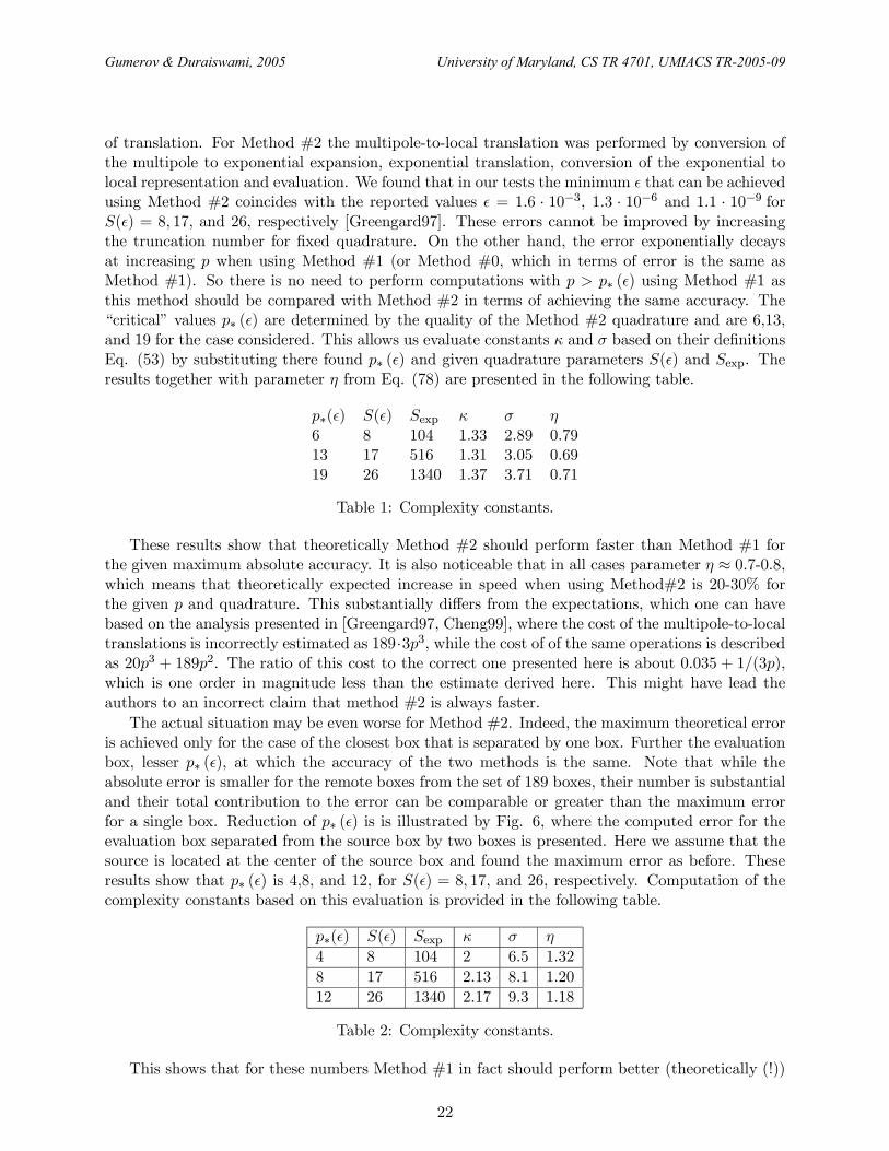
of translation. For Method #2 the multipole-to-local translation was performed by conversion ofthe multipole to exponential expansion, exponential translation, conversion of the exponential tolocal representation and evaluation. We found that in our tests the minimum ² that can be achievedusing Method #2 coincides with the reported values ² = 1.6 · 10−3, 1.3 · 10−6 and 1.1 · 10−9 forS(²) = 8, 17, and 26, respectively [Greengard97]. These errors cannot be improved by increasingthe truncation number for fixed quadrature. On the other hand, the error exponentially decaysat increasing p when using Method #1 (or Method #0, which in terms of error is the same asMethod #1). So there is no need to perform computations with p > p∗ (²) using Method #1 asthis method should be compared with Method #2 in terms of achieving the same accuracy. The“critical” values p∗ (²) are determined by the quality of the Method #2 quadrature and are 6,13,and 19 for the case considered. This allows us evaluate constants κ and σ based on their definitionsEq. (53) by substituting there found p∗ (²) and given quadrature parameters S(²) and Sexp. Theresults together with parameter η from Eq. (78) are presented in the following table.

p∗(²) S(²) Sexp κ σ η6 8 104 1.33 2.89 0.7913 17 516 1.31 3.05 0.6919 26 1340 1.37 3.71 0.71

Table 1: Complexity constants.

These results show that theoretically Method #2 should perform faster than Method #1 forthe given maximum absolute accuracy. It is also noticeable that in all cases parameter η ≈ 0.7-0.8,which means that theoretically expected increase in speed when using Method#2 is 20-30% forthe given p and quadrature. This substantially differs from the expectations, which one can havebased on the analysis presented in [Greengard97, Cheng99], where the cost of the multipole-to-localtranslations is incorrectly estimated as 189·3p3, while the cost of of the same operations is describedas 20p3 + 189p2. The ratio of this cost to the correct one presented here is about 0.035 + 1/(3p),which is one order in magnitude less than the estimate derived here. This might have lead theauthors to an incorrect claim that method #2 is always faster.

The actual situation may be even worse for Method #2. Indeed, the maximum theoretical erroris achieved only for the case of the closest box that is separated by one box. Further the evaluationbox, lesser p∗ (²), at which the accuracy of the two methods is the same. Note that while theabsolute error is smaller for the remote boxes from the set of 189 boxes, their number is substantialand their total contribution to the error can be comparable or greater than the maximum errorfor a single box. Reduction of p∗ (²) is is illustrated by Fig. 6, where the computed error for theevaluation box separated from the source box by two boxes is presented. Here we assume that thesource is located at the center of the source box and found the maximum error as before. Theseresults show that p∗ (²) is 4,8, and 12, for S(²) = 8, 17, and 26, respectively. Computation of thecomplexity constants based on this evaluation is provided in the following table.

p∗(²) S(²) Sexp κ σ η

4 8 104 2 6.5 1.32

8 17 516 2.13 8.1 1.20

12 26 1340 2.17 9.3 1.18


This shows that for these numbers Method #1 in fact should perform better (theoretically (!))

22


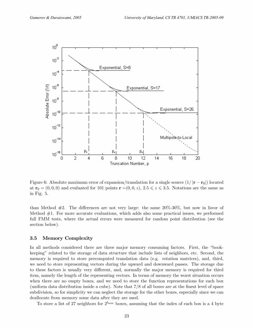
Figure 6: Absolute maximum error of expansion/translation for a single source (1/ |r− r0|) locatedat r0 = (0, 0, 0) and evaluated for 101 points r =(0, 0, z), 2.5 6 z 6 3.5. Notations are the same asin Fig. 5.

than Method #2. The differences are not very large: the same 20%-30%, but now in favor ofMethod #1. For more accurate evaluations, which adds also some practical issues, we performedfull FMM tests, where the actual errors were measured for random point distribution (see thesection below).

3.5 Memory Complexity

In all methods considered there are three major memory consuming factors. First, the “book-keeping” related to the storage of data structure that include lists of neighbors, etc. Second, thememory is required to store precomputed translation data (e.g. rotation matrices), and, third,we need to store representing vectors during the upward and downward passes. The storage dueto these factors is usually very different, and, normally the major memory is required for thirditem, namely the length of the representing vectors. In terms of memory the worst situation occurswhen there are no empty boxes, and we need to store the function representations for each box(uniform data distribution inside a cube). Note that 7/8 of all boxes are at the finest level of spacesubdivision, so for simplicity we can neglect the storage for the other boxes, especially since we candeallocate from memory some data after they are used.

To store a list of 27 neighbors for 2lmax boxes, assuming that the index of each box is a 4 byte

23


integer we need

M (1) = 27 · 2lmax · 4 (79)

bytes of storage.The memory required for storage of translation data depends on the method used. Since the

most consuming part is related to multipole-to-local translations we will neglect local-to-local andmultipole-to-multipole translation data in the memory storage. Assume that for Method #0 westore all S|R-translation matrices, which number is 343 for each level, and which contain p4 realentries occupying 8 bytes of memory each. In this case we need storage

M(2)0 = 343p4 · (lmax − 1) · 8. (80)

For Method #1 there are 15 different translation distances for each level and the coaxial S|Rtranslation matrix requires ≈ p3/3 storage of real numbers. In addition there are 48 different non-zero rotation angles β. Taking into account that storage of the rotation matrix requires ≈ 2p3/3real numbers, and the rotation matrices are the same for all levels, we have the memory complexity

M(2)1 = 15

p3

3· (lmax − 1) · 8 + 48

2p3

3· 8 = 8p3 (5lmax + 27) . (81)

For Method #2 the storage of precomputed translation data can be done with memory complexity

M(2)2 = 8S (²)

µ3Sexp +

p2

2

¶(lmax − 1) +

2p3

3· 8. (82)

Finally, the storage of representations of length p2 for Methods #0 and #1 at level lmax requires

M(3)0,1 = 2 · 2lmaxp2 · 8 (83)

bytes, where factor 2 appears due to storage of both multipole and local coefficients is needed. ForMethod #2 we need at least

M(3)2 = 2lmaxSexp · 8 + 2 · 2lmaxp2 · 8 (84)

bytes, where the first number is related to functions representation via exponential expansion, andthe second number is the minimum needed to store the multipole and local expansions.

For Methods #1 and #2 the storage of translation data is much smaller than the storage ofrepresentations, while for Method #0 this can be substantial. We also can neglect the storageof the neighbor list. With such simplifications and using Eq. (53) we can evaluate the memoryrequirements for Methods #1 and #2 as follows:

M1 ≈ M(3)1 = 16 · 2lmaxp2, (85)

M2 ≈ M(3)2 = 16 · 2lmaxp2

µ1 +

1

2σ

¶.

This shows that e.g. for σ = 3 the ratio M2/M1 = 2.5. This shows a substantial increase of thememory complexity for Method #2 compared to Method #1. Thus a strong advantage for Method#1 relative to Method #2 is that for a given memory size it can fit a larger problem.

24


3.6 Possible Reductions of Asymptotic Constants

We note that there are several opportunities to reduce the number of operations in conversion forMethod #2. One of them is related to the observation that the conversions S|E and E|R involvesums of complex exponents, and, in fact are Fourier transforms of periodic functions. One canexploit some ideas of the FFT (the Danielson-Lanczos lemma) to reduce the complexity of thedirect summation. We tried one-step reductions using this lemma and found that the overall speedcan be improved by a few percents. Another opportunity is to use some symmetries to reduce theasymptotic constant 189. Greengard and Rokhlin [Greengard97] mention that there may be suchpossibilities, but do not provide them, and their results in [Greengard97] and [Cheng99] appear tonot use such symmetries. Some savings can be done for cases of low p when in some places of thecode single precision real numbers can be used instead of double precision without substantial lossof accuracy. We also should mention, that if some symmetries are used for translations in Method#2, then symmetries for Methods #0 and #1 also should be considered more carefully. E.g. thetranslation matrix can be decomposed to a sum of two matrices (half of elements of each are zeros)so the translation with vector t can be done using a sum of these matrices, while translation indirection −t can be done using the difference. In the numerical tests provided below we did notuse the above-mentioned opportunities.

4 Numerical tests

The problem that was solved in the numerical tests is related to potential N -particle interaction(e.g. gravity or electrostatic forces) and is the same as in [Cheng99]. Here we compute

φ (rj) =NX

i=1,i6=jqiG(ri, rj), j = 1, ..., N, (86)

where qi are the source intensities, which in tests were set all equal. The sources were randomlyuniformly distributed inside a cube (say, the unit cube, since the Laplace equation does not haveits own scale and all results can be scaled to the domain of arbitrary size).

The code was realized in Fortran 90 and compiled using the Compaq 6.5 Fortran compiler. Allcomputations were performed in double precision. In the tests we used the version of the FMMfor real functions. The CPU time measurements were conducted on a 3.2 GHz dual Intel Xeonprocessor with 3.5 GB RAM. Some particulars of our implementation are mentioned in the previoussection. Different translation methods were implemented in the same programming environmentand most subroutines used (except of specific translation subroutines) were the same, which enablesus to conduct a comparison of performance of those methods. We also paid attention to efficiencyof implementation trying to use the fastest computational algorithms for each method. We alsocompared our implementation with the “cross-over" points of other implementations reported inthe literature.

4.1 Computation of errors

To compare the FMM utilizing different translation methods first we introduce the measures forthe errors. If there are M evaluation points in the domain, the absolute errors in the L∞ and L2

25


norms are

²(abs)∞ = maxj=1,...,M

¯φexact (rj)− φapprox (rj)

¯, ²

(abs)2 (87)

=

⎡⎣ 1M

MXj=1

¯φexact (rj)− φapprox (rj)

¯2⎤⎦1/2 ,where φexact (r) and φapprox (r) are the exact and approximate solutions of the problem. Theabsolute errors, however, are not representative, since they depend on the scaling of the sourceintensities. To introduce scale independent relative errors, we can select some representative scale,e.g. some norm of the exact solution. The scale can be selected as the L2 norm of function φexact (r):

kφexact (r)k2 =

⎡⎣ 1M

MXj=1

|φexact (rj)|2⎤⎦1/2 . (88)

So the absolute errors were related to this scale:

²∞ =²(abs)∞

kφexact (r)k2, ²2 =

²(abs)2

kφexact (r)k2. (89)

The exact solution was computed by straightforward summation of the source potentials (86).This method is acceptable for relatively low M , while for larger M the computations becomeunacceptably slow, and the error can be measured by evaluation of the errors at smaller number ofthe evaluation points. Figure 7 shows comparison of the ²∞ and ²2 errors computed over the full setof the evaluation points and over the first 100 points. It is seen that the errors in the L2 norm arealmost the same for these two cases, while a difference is observed for the errors in the L∞ norm.While this difference seems is not very large and further we will use smaller number of the evaluationpoints to estimate the error (especially when we concern about the orders of magnitude), we shouldstate that ²∞ computed over first 100 random points represents some probabilistic measure andnot exactly ²∞, which can be larger.

4.2 Error dependence

The errors specified above depend on several factors, including the number and location of thesources, the translation method used, the truncation number, and the number of levels in theFMM. Since the accuracy of Methods #0 and #1 is the same in terms of error dependences, onlyMethods #1 and #2 are compared.

For the fixed distribution of N sources we can consider dependence of the errors on the trunca-tion number p and the maximum level of space subdivision lmax used in the FMM. Concerning thelatter dependence we note that this dependence is much weaker than the error dependence on thetruncation number. So for any level and given truncation number we have approximately the sameerror. On the other hand the dependence of the error on p is strong and qualitatively different forMethod #1 and Method #2. Figure 8 shows dependences of ²2 and ²∞ on p for fixed N and lmax.Qualitatively he behavior is similar to that for absolute errors shown in Figs. 5 and 6. We note thatp∗ depends on the norm in which the error is measured. This “critical” truncation number is largerif ²∞ is used. Based on the L2 norm, which is confirmed by the performance study the criticaltruncation numbers are p∗ = 4, 9, and 19. For these numbers the following theoretical complexityconstants are expected.

26


0.E+00

1.E-04

2.E-04

3.E-04

4.E-04

5.E-04

6.E-04

100 1000 10000 100000N

Rel

ativ

e E

rror

Linf

L2

M=N

M=N

M=100

M=100

Figure 7: The relative errors ²∞ (marked as Linf) and ²2 (marked as L2) computed accordingEq. (89) for the full set of evaluation points (M = N) and for the first 100 evaluation points(M = 100). Computations performed for translation scheme using exponential expansions, p = 6,lmax = 3, sources of equal intensity are randomly distributed inside a cube.

Figure 9 illustrates dependence of the error on the size of the problem N . According the theory,the absolute error of the multipole expansions decays exponentially at the growing p. Assumingthat each source contributes equally to the total absolute error we can state then that to providea constant absolute error we should have p ∼ logN . For computation of the solid curve shownin Fig. 9 we used the Method #1 with p = log2N + 2. It is seen that the absolute error ²(abs)2

does not increase in this case, that is consistent with the theory. Figure 9 also shows that for theincreasing N the norm of function kφexact (r)k2 grow proportionally to N . The same is true for theabsolute error ²(abs)2 if computations are performed at constant p. This means that the relative error²2 stays stably within some bound at constant p. So if the purpose of computations is to obtainsolution with some prescribed relative error, then this can be done using constant p (in which casethe FMM is an O(N) algorithm). Figure 9 illustrates this fact for computations using Method #1and Method #2, where for Method #2 we selected p = p∗ (for the relative L2 error as provided byFig. 8). Note that we also computed errors ²(abs)∞ and ²∞ for the same settings. While these errorsare several times higher than ²(abs)2 and ²2, respectively, their qualitative behavior is the same asfor the errors in the L2 norm. While some discrepancy is observed for errors computed by the twotranslation methods at p = 9, errors ²(abs)∞ and ²∞ are almost the same for these methods. This is

27


p∗(²) S(²) Sexp κ σ η4 8 104 2 6.5 1.329 17 516 1.89 6.4 1.0519 26 1340 1.37 3.7 0.71


explainable by Fig. 8.

4.3 Optimization

We formulate the optimization problem as follows. The optimum performance means the settingwhich achieves the minimum of the CPU time required for computation of a given problem (afixed source distribution) at the constraint that the error is smaller than some prescribed error.We measured the CPU time only for the “run” time of the algorithm, which, first, has the majorcontribution to the overall CPU time, compared to the preset step (which is also sensitive tothe way of implementation of data structures). By this definition the optimum performance candepend on the norm in which the error is measured. Once the source distribution is fixed only twoparameters, p and lmax can be varied. When using Method #2 with some fixed order quadrature,we understand that the error cannot be arbitrary, but it should be not less than the minimumerror provided by this order of quadrature. In this case to compare performance of the FMM withdifferent translation methods we set p = p∗ and then optimize lmax to achieve the minimum CPUtime for Method #2. This determines the error of the method at this optimum lmax. Then forMethod #0 and Method #1 we solve an optimization problem to determine p (which, presumably,is the same as p∗) and lmax that provide the same error as the error of Method #2 (or close to that— the criteria for computations with the same error in practice can be relaxed assuming that, say,two errors differ not more than 30% or 50% they are the same).

Figure 10 illustrates selection of the optimum maximum level. Here first CPU time was mea-sured for Method #2 at different lmax, which shows that for given p = 9 (p∗ = 9 for the relativeerror in the L2 norm) the optimum lmax = 4. At this optimum we found that ²2 = 1.22 ·10−7 (mea-sured over first 100 evaluation points). Further we did similar tests using Method #0 and Method#2 for p = 9 and found that for Method #0 the optimum lmax = 3, at which ²2 = 7.15 · 10−8,while for Method #1 the optimum achieves at lmax = 4, in which case ²2 = 7.44 · 10−8. Thenwe performed computations with p = 8 and found that the errors in this case (²2 = 3.01 · 10−7for Method #1 and ²2 = 2.77 · 10−7 for Method #0 at optimum levels) are substantially larger(more than 50%) than for Method #2 and p = 9. So we conclude that the optimal settings forcomputations with prescribed error ²2 ∼ 10−7 for all methods are p = 9 and lmax = 3 for Methods#0 and lmax = 4 for Method #1 and #2 .

To conduct further comparative performance study, we conducted similar optimization for allreported cases. Some insight to optimization problem at constant p is provided in the theoreticalsection, where it is shown that in this case the optimum theoretically should be achieved at thesame values of the clustering parameter s. We checked this with the current code and found thatthis is a valid statement. In any case we varied the clustering parameter, which affects only lmaxto be sure that indeed the optimum setting is provided for every random distribution.

It is also noticeable that figures in our implementation are close to the theoretical predictions.For example, for p = 9, Eqs. (67), (42), and (75) predict sopt = 130 for Method #1 and sopt = 128for Method #2 (which is almost the same, since this determines the same lmax). we found thatcomputations with s = 128 (we varied this parameter by doubling) are indeed optimal for the

28


range of levels lmax = 2, ..., 6. Fig. 10 also shows that Methods #1 and #2 performs almost thesame. This agrees with the theoretical estimate (in the previous section we found that the ratio ofmethods costs is η = 1.05, which is very close to 1 for case p = 9, S (²) = 17.

4.4 Performance study

We conducted performance study for three cases of “low”, “moderate”, and “large” truncationnumbers corresponding to the accuracy provided by the quadrature formula using different transla-tion methods. These correspond to the cases considered in [Greengard97]. As we mentioned abovethe CPU time was measured only for the “run” part of the algorithm, which opposed to the presetstep should be performed only once if the point distribution does not change.

4.4.1 Low accuracy

In this case when using Method #2 we employed the quadrature formula of order 8. Figure 11illustrates error dependences on N for the optimized FMM with different translation methods anddifferent truncation numbers. This shows that when using Method #2 we have p∗ = 4.

Indeed, in this case computations with p = 4 and p = 5 yield the same order of the error, andthere is no improvement in accuracy for larger p both for the ²2 and ²∞ errors. On the other hand,the errors obtained when using Method #1 while slightly higher are about the same as the errorsfor Method #2 for p = 4. Computations with p = 5 and Method #1 provide substantially smallererrors compared to computations using p = 4 and p = 5 and Method #2.

Figure 12 illustrates the performance of the optimized FMM using different translation methods.As it is seen at low truncation numbers all the methods require about the same time to computethe same problem. Method #1 at p = 4 is a bit faster than the other methods. Increase of pto p = 5 increases the CPU time and, in fact makes Method #1 a bit slower than Method #2.This is consistent with the above theory, which predicts the ratio of speeds η > 1 for p = 4 andη < 1 for p = 5. This figure also shows that our implementation of the FMM is pretty efficient,since all the methods perform faster than the direct, or straightforward, summation for N > 103(in fact, the break-even point, N∗, is 2-3 times smaller than N = 103; for p = 4 and Method #0we found N∗ = 380, Method #1 yields N∗ = 320 for the same p, and Method #2 for p = 4 andthe S (²) = 8 has N∗ = 430, which is somehow lower than N∗ = 750 reported in [Cheng99] forthis method with the same accuracy (presumably larger p was used in the cited reference, also thebreak-even point depends on the implementation; we also note the folowing differences: in the citedpaper computations were made with a single precision, and it is not clear whether the total CPUtime or the CPU time for the “run” part of the FMM is measured).

4.4.2 Moderate accuracy

In this case when using Method #2 we employed the quadrature formula of order 17. Figure 13illustrates error dependences on N for the optimized FMM similarly to Fig. 11. This shows thatwhen using Method #2 we have p∗ = 9. Indeed, the use of p = 10 does not improve the ²2 error forMethod #2. At the same time computations with p = 9 using Method #1 have errors ²2 smallerthan those for Method #2, while for p = 10 the errors for Method #1 are several times smallerthan that for Method #2.

Figure 14 shows the CPU time measurements for the optimized FMM employing differenttranslation schemes. This comparison shows that at higher N Method #1 and Method #2 requireabout the same time for computation of the same problem with the same accuracy, while Method

29


#1 is slightly faster at lower N and slightly slower at larger N . The difference of speed of Method#1 and Method #2 is really small. For example, computation of N = 220 ≈ 106 problem takes 112seconds for Method #1, while 105 seconds for Method #2, which is just 6% better. Such differencesnormally should not be taken into account, since different implementation may change the situationto the opposite (we tried to implement each method in the fastest way). It is interesting to notethat for p = 9 in our implementation the break-even points are about N∗ = 1800, 900, and 1100for Method #0, #1, and #2, respectively. Note that the break-even point N∗ = 1500 reported in[Cheng99] for Method #2.

Being O(p4) Method #0 at high N slows down several times compared to the O(p3) translationmethods, which is an expected result. So, while this method is comparable with the other twomethods for low accuracy computations, for higher accuracy it loses the competition at least toMethod #1, which has just the same accuracy, but is substantially faster. We note that theseresults show that the improvement achieved by method 1 are better than that reported in theoriginal paper [White96], and close to the predicted improvement. Our results for low accuracyfrom the previous subsection also show that there is no any advantage for using Method #0 evenin the case p = 4 (however we checked that for p = 3 Method #0 is in some cases slightly fasterthan the O(p3) methods).

4.4.3 High accuracy

In this case when using Method #2 we employed the quadrature formula of order 26. Figure 15illustrates error dependences on N for the optimized FMM similarly to Fig. 11. This shows thatwhen using Method #2 we have p∗ = 19. Indeed, the use of p = 20 does not improve ²2 errors forMethod #2. Error ²2 for Method #1 with p = 19 is comparable with ²2 for Method #2 at lowerN and much smaller at larger N (so smaller p∗ can be used in this case). Fig. 19 shows that theuse of p∗ = 16 provides larger error, while p∗ = 17 can be used for large N .

Figure 16 is similar to Figs.12 and 14. As in the previous figures we can see that the FMM usingMethod #1 and Method #2 spend approximately the same time for solving the same problem withthe same accuracy. At lower N Method #1 is slightly faster than Method #2, while for larger NMethod #2 is faster than Method #1. For example to compute the problem with N = 213 ≈ 104the FMM run times for Methods #1 (p = 19) and #2 are 1.2 and 1.25 seconds, respectively. ForN = 221 ≈ 2 · 106 the CPU times for Methods #1 (p = 19) and #2 are 665 and 502 seconds,respectively, i.e. Method #2 performs 25% faster than Method #1 (for larger N the ratio variesfrom 10 to 35%, since the optimal level for Method #2 should be lower than for Method #1, butsince the level can be only an integer, some non-optimal performance cannot be avoided, which isconsistent with the 29% difference predicted by the theory). The use of variable p improves thespeed of Method #1 at larger N , in which case Method #2’s performance advantage is at most25% over Method #1 for any N). We also note that the break-even point with the direct methodincreases in our implementation up to approximately N∗ = 2500 for both Methods #1 and #2.This coincides with the break-even point N∗ = 2500 reported in [Cheng99]. Concerning Method#0 it should be noted, that it is not competitive for computations with high accuracy (also noticeits high break-even point for Method #0, N∗ > 10000).

Figure 17 demonstrates the CPU time required for the performance of the FMM (the samedata as in Fig. 16) and for presetting of the FMM run (computation related to data structure andprecomputation of the translation operators). The latter step should be performed only once as thedata points do not change, while the former step can be performed many times (e.g. in iterativesolvers). It is seen that the preset step normally takes only several percents of the FMM run timeand the cost of this step is approximately the same for Methods #1 and #2. The preset time

30


mainly depends on the maximum level of space subdivision in the FMM, that is why the graphlooks like a staircase function, where the jumps occur when lmax changes (in the case reported foroptimal performance lmax changed from 2 to 5 and those changes are clearly seen on the graph forthe FMM preset time). Finally we note that the CPU time to preset the FMM in the case of highaccuracy computations at large N is about two orders of magnitude of the run time.

4.5 Discussion

The results of the performance study show that while the FMM using translation Method #1 ortranslation Method #2 can be slightly faster, the both O(p3) methods provide the same order speedand accuracy. The behavior observed in practice is consistent with the theoretical estimates, whichcan be used to predict relative algorithm performance.

Another issue affecting the performance is that the memory required for Method #2 is largerthan for Method #1. The increase of the memory for Method #2 compared to Method #1 is about1 + σ/2 times (with σ given in the tables in the previous sections). This affects not only the issueof RAM availability for the task and limits the size of the problems that can be solved on a givenCPU, but also affects the speed of retrieval and storage of data required in the process of algorithmexecution (we checked this by profiling of the programs). Indeed the multipole-to-local translationoperation can be performed millions times and in this count increase of the local data size can besignificant compared to the overall count of operations, which may modify the asymptotic constantsfor each method.

5 Conclusions

We implemented the FMM with the original O(p4) and two O(p3) translation schemes (the “point-and-shoot” method of [White96] and the exponential translation scheme of [Greengard97, Cheng99])in the same programming environment and conducted comparative performance study in terms ofthe speed of the FMM that achieves the same prescribed error. This study showed that:

1). Low relative errors in the L2 norm (evaluated over 100 random points) can be achieved atrelatively low truncation numbers p.

2). For low accuracy computations (²2 ∼ 10−4) all the translation schemes have almost thesame performance, while the “point-and-shoot” method is slightly faster then the other methodsconsidered here. For this accuracy, we note that treecodes are competitive as well, and may be themethod of choice.

3) For moderate accuracy (²2 ∼ 10−7) the original FMM (O(p4)) is several times slower thanO(p3) methods tried, which have about the same performance. For high accuracy (²2 ∼ 10−10) theO(p4) method is substantially slower than the O(p3) translation methods. In this case both O(p3)methods perform approximately with the same speed. For high accuracy computations the “point-and-shoot” method is slightly faster for lower N (N . 104), while the method using the exponentialexpansions for the multipole-to-local translations is faster for higher N (105 6 N 6 106). Thedifference between the speed of the methods performing with the same accuracy (for maximumaccuracy achievable by a given quadrature) is within 25% with respect to the speed of the “point-and-shoot” method for computed benchmark cases.

4) The memory required for the exponential translation is significantly higher.5) The observed performance is explained by several factors. First, the number of terms in the

multipole expansions p2 that can be used to achieve the same errors as provided by the quadratureorder for the exponential expansion are several times smaller than the number of terms in theexponential expansion, Sexp. Second, more accurate complexity estimates show that previously

31


reported complexity constants for the method using the exponential expansion are underestimated.Third, there exist a necessary overhead which slow down the method based on the exponentialexpansion due to Sexp > p2. Finally, the memory required for Method #2 is larger than forMethod #1.

6 Acknowledgments

Partial support of NSF awards 0086075 and 0219681 is gratefully acknowledged. We thank Dr.Peter Teuben for discussions regarding tree codes.

References

[Abramowitz65] M. Abramowitz, and I. A. Stegun, Handbook of Mathematical Functions, DoverPublications, 1965.

[Barnes86] J. Barnes and P. Hut, A hierarchical O(N logN) force-calculation algorithm, Na-ture, 324, 1986, 446-449.

[Carrier88] J. Carrier, L. Greengard, and V. Rokhlin, A fast adaptive multipole algorithm forparticle simulations, SIAM J. Sci. Statist. Comput., 9, 1988, 669-686.

[Cheng99] H. Cheng, L. Greengard, and V. Rokhlin, A fast adaptive multipole algorithm inthree dimensions, J. Comput. Phys., 155, 1999, 468-498.

[Dehnen02] W. Dehnen, A Hierarchical O(N) force calculation algorithm, J. Comput. Phys.179, 2002, 27—42.

[Elliott02] W. Elliott and J. Board, Jr., Fast Fourier transform accelerated fast multipolealgorithm, SIAM J. Sci. Computing, 17(2), 1996, 398-415.

[Epton95] M.A. Epton and B. Dembart, Multipole translation theory for the three-dimensional Laplace and Helmholtz equations, SIAM J. Sci. Comput., 16(4), 1995,865-897.

[Greengard88] L. Greengard, The Rapid Evaluation Of Potential Fields in Particle Systems, MITPress, Cambridge, 1988.

[Greengard87] L. Greengard and V. Rokhlin, A fast algorithm for particle simulations, J. Comput.Phys., 73, 1987, 325-348.

[GreengardL88] L. Greengard and V. Rokhlin, Rapid evaluation of potential fields in three di-mensions, in Vortex Methods. Edited by C. Anderson and C. Greengard. LectureNotes in Mathematics, Springer-Verlag, Berlin, 1360, 1988, 121-141.

[Greengard97] L. Greengard and V. Rokhlin, A new version of the fast multipole method for theLaplace equation in three dimensions, Acta Numerica, 6, 1997, 229-269.

[Gumerov2003] N.A. Gumerov, R. Duraiswami, and E.A. Borovikov, Data structure, optimalchoice of parameters, and complexity results for generalized multilevel fast mul-tipole methods in d dimensions, UMIACS TR 2003-28, University of Maryland,College Park, 2003.

32


[Gumerov2005] N.A. Gumerov and R. Duraiswami, Fast Multipole Methods for the HelmholtzEquation in Three Dimensions, Elsevier, Oxford, 2004.

[Hrycak98] T. Hrycak and V. Rokhlin, An improved fast multipole algorithm for potentialfields, SIAM J.Sci. Comput., 19(6), 1998, 1804-1826.

[Lindsay01] K. Lindsay and R. Krasny, A particle method and adaptive treecode for vortexsheet motion in three-dimensional flow, J. Comput. Phys., 172, 2001, 879-907.

[Ong04] E.T. Ong, H.P. Lee, and K.M. Lim, A parallel fast Fourier transform on mul-tipoles (FFTM) algorithm for electrostatics analysis of three-dimensional struc-tures,” IEEE Trans. Computer-Aided Design of Integrated Circuits and Systems,23, 2004, 1063-1072.

[Petersen94] H.G. Petersen, D. Soelvason, and J.W. Perram, The very fast multipole method,J. Chem. Phys. 101(10), 1994, 8870-8876.

[Rokhlin83] V. Rokhlin, Rapid solution of integral equations of classical potential theory, J.Comput. Phys., 60, 1983, 187-207.

[Tang03] Z. Tang, Fast Transforms Based On Structured Matrices with Applications to theFast Multipole Method, Ph.D. thesis, University of Maryland, College Park, 2003.

[White96] C.A. White and M. Head-Gordon, Rotation around the quartic angular momentumbarrier in fast multipole method calculations, J. Chem. Phys., 105(12), 1996, 5061-5067.

33


1.E-14

1.E-12

1.E-10

1.E-08

1.E-06

1.E-04

1.E-02

1.E+00

0 5 10 15 20 25 30Truncation Number, p

Rel

ativ

e E

rror Linf

L2

11

2(8)

2(17)

2(26)

N=65536l max = 4

Figure 8: The relative errors ²∞ (marked as Linf) and ²2 (marked as L2) computed according Eq. (89) for the first 100 evaluation points (M = 100) as functions of the truncation number, p. The solidand dotted curves show computations using translation method #1, while the triangles, squaresand discs correspond to computations using translation method #2 (exponential expansions). Inthe latter case the numbers in the parenthesis after 2 show the order of quadrature, S (²), usedfor exponential representation. 65536 sources of equal intensity are randomly distributed inside acube; lmax = 4. Computations with double precision.

34


1.E-08

1.E-06

1.E-04

1.E-02

1.E+00

1.E+02

1.E+04

1.E+06

1.E+02 1.E+03 1.E+04 1.E+05 1.E+06 1.E+07Number of Sources, N

Erro

rs, N

orm

in L

2

Exact solution norm

Absolute error, p=9

Relative error p=9

Absolute error, p=log2N+2

1

2

2

1

1

Figure 9: Dependences of the exact solution L2 norm (the dash-dotted line) and absolute andrelative errors in the L2 norm (solid and dashed lines) on the size of the problem, N . The translationmethod used is indicated near the curves. In the Method #2 the quadrature of order 17 was used.The discs connected by the solid line show the absolute error for computations using p dependingon N as shown. The squares and triangles connected by the dashed line show computations usingconstant p = 9.The sources of unit intensity are uniformly randomly distributed inside the unitcube. Error is measured based on the first 100 evaluation points.

35


1

10

100

1000

1 2 3 4 5 6Maximum Level in the FMM

CP

U T

ime

(s)

12

0

N=65536, p=9

Figure 10: Dependence of the CPU time (Intel Xeon 3.2 GHz, 3.5 GB RAM) on the maximum levelof space subdivision used in the FMM. Numbers near the curves indicate the translation methodused (for Method #2, S(²) = 17). Sources of equal intensity are randomly uniformly distributedinside a cube.

36


1.E-05

1.E-04

1.E-03

1.E+03 1.E+04 1.E+05 1.E+06 1.E+07Number of Sources, N

Rel

ativ

e E

rror

M#1, p=4, L2M#2, p=4, L2M#1, p=5, L2M#2, p=5, L2

Figure 11: The relative errors ²2 (data series are connected by the solid lines) as functions ofthe number of sources for computations with the FMM using different translation methods (thetriangles for Method #1, and the discs for Method #2 with the 8th order quadrature) for truncationnumbers p = 4 (the empty marks) and p = 5 (the filled marks). Error measurements are made overthe first 100 evaluation points. The maximum level in the FMM is optimized for each N . Sourcesare distributed uniformly randomly inside a cube. Computations are made with double precision.

37


0.001

0.01

0.1

1

10

100

1000


CP

U T

ime

(s)

DirectMethod #0Method #1Method #2Method #1, p=5

p=4 y=axy=bx2

Direct

FMM

Figure 12: The CPU time in seconds required for computation of problems of size N using differentmethods. Data shown by filled rhombi corresponds to the direct solution, which complexity is scaledas O(N2) shown by the dashed line y = bx2. FMM computations using Methods #0, #1, and #2with truncation number p = 4 are shown by the empty squares, triangles, and discs, respectively.FMM computations using Method #1 and p = 5 are shown by smaller filled triangles. All the FMMcomputations are scaled asymptotically linearly at larger N . The dashed line y = ax presents linearscaling. CPU is measured for the Intel Xeon 3.2 GHz processor, 3.5 GB RAM (double precision).

38


1.E-08

1.E-07

1.E-06


Rel

ativ

e E

rror

M#1, p=9, L2M#2, p=9, L2M#1, p=10, L2M#2, p=10, L2

Figure 13: The same as Fig. 11 but for different truncation numbers and Method #2 using the17th order quadrature.

39


0.01

0.1

1

10

100

1000


CP

U T

ime

(s)

DirectMethod #0Method #1Method #2

p=9

y=axy=bx2

Direct

FMM

Figure 14: The same as Fig. 12, but for different p (p = 9) and for the 17th order quadrature forMethod #2.

40


1.E-11

1.E-10

1.E-09


Rel

ativ

e E

rror

M#1, p=19M#2, p=19M#2, p=20M#1, p=19…17M#1, p=16

Figure 15: The same as Fig. 11 but for different truncation numbers and Method #2 using the26th order quadrature. The curve marked by the dark triangles corresponds computed for variablep (p = 19 for N = 210; p = 18 for N = 210 − 215; p = 17 for N = 216 − 222).

41


1.E-01

1.E+00

1.E+01

1.E+02

1.E+03

1.E+04


CP

U T

ime

(s)

DirectMethod #0Method #1Method #2Method #1 (variable p)

p=19

y=axy=bx2

Direct

FMM

Figure 16: The same as Fig. 12, but for different p (p = 19) and for the 26th order quadraturefor Method #2. The dark triangles show performance of Method #1 where p can be reduced forparticular N according the error in the L2 norm (see Fig. 19).

42


1.E-02

1.E-01

1.E+00

1.E+01

1.E+02

1.E+03


CP

U T

ime

(s)

Method #1 (run)Method #2 (run)Method #1 (preset)Method #2 (preset)

p=19

y=ax

FMM (run) y=bx

FMM (preset)

Figure 17: Depenedences of the CPU time for the preset and the run step of the FMM. p = 19,S (²) = 26.

43


Comparison of the e ﬃciency of translation operators used ...

Documents

Transcript of Comparison of the e ﬃciency of translation operators used ...