Comparison of superresolution algorithms with different ... · Calhoun: The NPS Institutional...

Calhoun: The NPS Institutional Archive

Theses and Dissertations Thesis Collection

1998-09

Comparison of superresolution algorithms with

different array geometries for radio direction finding

Lin, Ku-Ting

Monterey, California. Naval Postgraduate School

http://hdl.handle.net/10945/8125

•LEY KNOX LIBRARYAl POSTGRADUATE SC!•JTFREY C/ VS101

NAVAL POSTGRADUATE SCHOOLMonterey, California

THESIS

COMPARISON OF SUPERRESOLUTION ALGORITHMSWITH DIFFERENT ARRAY GEOMETRIES FOR

RADIO DIRECTION FINDING

by

Ku-Ting Lin

September 1998

Thesis Advisor:

Second Reader:

David C. Jenn

Phillip E. Pace

Approved for public release; distribution is unlimited.

Approved for public release; distribution is unlimited.

COMPARISON OF SUPERRESOLUTION ALGORITHMSWITH DIFFERENT ARRAY GEOMETRIES FOR

RADIO DIRECTION FINDING

Ku-Ting Lin

Chung-Shan Institute of Science and Technology, Taiwan

B.S.EE., Chung-Cheng Institute of Technology, Taiwan, 1990

Submitted in partial fulfillment

of the requirements for the degree of

MASTER OF SCIENCE IN ELECTRICAL ENGINEERING

from the

NAVAL POSTGRADUATE SCHOOLSeptember 1998

ABSTRACT

The objective of this thesis is to investigate and

evaluate the effectiveness of modern estimation methods

with different array geometries as they apply to the

problem of bearing estimation. The algorithms were

selected from those that apply to multidimensional case,

including MUSIC, PHD, minimum norm, and Capon' s beam-

former. These four techniques were chosen based on their

high resolution capability, and their ability to deal with

three-dimensional non-uniform arrays and to estimate both

azimuth and elevation angle of arrival (AOA) . Computer

simulations were run for linear arrays, circular arrays,

and combinations of the two. The test conditions included

(1) two closely spaced emitters, and (2) various levels of

additive white Gaussian noise.

v

TABLE OF CONTENTS

I . INTRODUCTION 1

A. OVERVIEW 1

B. THESIS OUTLINE 6

1 1 . ANTENNA ARRAY 7

A. UNI FROM LINEAR ARRAY 7

B. NON-NUI FORM LINEAR ARRAY (MINIMUM-REDUNDANCY) .. 10

C . CIRCULAR ARRAY 11

D. SPIRAL ARRAY 14

E. COMBINATION OF LINEAR AND CIRCULAR ARRAYS 14

III

.

SPATIAL SPECTRUM ESTIMATION 17

A. MUSIC 17

B. ESPRIT 20

C

.

BEAMFORMING 22

1 . Conventional Beamformer 22

2 . Capon' s Beamformer 24

D. PHD 25

E

.

MINIMUM NORM METHOD 2 6

IV. IMPLEMENTATION AND COMPUTER CODES 29

A. PARAMETERIC DATA MODEL AND FLOWCHART 2 9

1. Input Parameters 29

VII

2. Signal and Noise Models 313

.

Antenna Array Model 324. Correlation Matrix and Spatial SpectrumMethods 34

B. THE IMPLEMENTATION OF ARRAY MATRIXDECOMPOSITION 35

C. GRAPHICAL USER INTERFACE 37

V. SIMULATION RESULTS AND ANALYSIS 39

A. ANGULAR RESOLUTION of ONE-DIMENSIONAL DF 39

B. TWO-DIMENSIONAL DIRECTION FINDING 40

1 . Azimuth Angular Resolution 402 Elevation Angular Resolution 47

3. Multiple Signal Sources 47

4

.

Comparison of Azimuth and Elevation AngularResolution 525. Improvement of Angular Resolution of Two-dimensional DF 52

VI . CONCLUSIONS 61

APPENDIX A - THESIS MAIN PROGRAM 65

APPENDIX B - SPECTRUM CALCULATION FOR CIRCULAR ARRAY 75

APPENDIX C - SPECTRUM CALCULATION FOR SPIRAL ARRAY 79

APPENDIX D - SPECTRUM CALCULATION FOR CIRCULAR+LINEAR

ARRAY 8 3

APPENDIX E - SPECTRUM CALCULATION FOR LINEAR ARRAY 87

Vlll

APPENDIX F - SPECTRUM CALCULATION FOR NON-UNIFORM LINEAR

ARRAY 8 9

LIST OF REFERENCES 91

INITIAL DISTRIBUTION LIST 93

IX

ACKNOWLEDGMENT

I would like to acknowledge my thesis advisor,

Professor David C. Jenn for his guidance and encouragement.

Most of all, I would like to thank my wife, Seli and

my daughter, Grace for their love, support and

understanding

.

XI

I . INTRODUCTION

A. OVERVIEW

The angle of arrival (AOA) is a valuable parameter to

be used in deinterleaving signals because a target can not

change its position rapidly. Even an airbone radar can not

significantly change its position in the few milliseconds of

the waveform pulse repetition interval (PRI) time. As a

result, the AOA measured by an intercept receiver on the

radar is relatively stable value. It requires that a large

number of antenna elements and receivers must be matched,

either in amplitude or in phase in order to measure the AOA.

Direction finding (DF) is the area of electronic-

warfare support whose objective is to find the AOA [Ref . 1]

.

DF systems passively examine the spectrum use by hostile

emitters and process the signals to obtain enemy AOA

information.

The two common approaches to measure AOA are based on

amplitude and phase comparison [Ref. 1] . The phase

comparison system usually can generate AOA resolution of ±1

degree, which satisfies the modern EW requirement. The

number of antennas that can be used in an AOA system is very

low in comparison with electronically scanning antennas in a

radar system. In an airbone system, the maximum number of

elements might be ten. In a ship-based system, the number

might be larger.

For the phase comparison method at least two separate

antenna elements with a predetermined space between them are

required. Since the distances from the emitter to the two

elements are not the same (except in the broadside case),

the incident wave arrives at the two elements after

traveling uneven paths, and thus it arrives with a different

phase. The phase delay is proportional to the antenna

spacing, wavelength and angle of incidence. Since the first

two factors are constant, the direction information can be

obtained.

DF systems often receive signals from several sources

in the same frequency range at the same time and from many

different angles of arrival. To resolve multicomponent

wavefields, modern techniques of spectral estimation are

used. Most recent digital AOA studies have concentrated on

high-resolution approaches, such as the MUSIC, ESPRIT and

minimum norm methods [Refs. 2-4] . In this thesis the

performance of several modern estimation methods is

evaluated for different array geometries. This research

deals with both the one- and two-dimensional problems:

azimuth angle of arrival for linear arrays, and azimuth and

elevation angles for a planar array. In addition, an

underlying assumption is that the receiver is far enough

from the transmitter and the antenna interactions with the

platform are controlled so that the arriving wavefront is

essentially planar.

The main function of a direction finder is to determine

the direction of arrival of an incident electromagnetic wave

relative to the coordinates of the direction finding site

[Ref . 1] . Figure 1 shows a representative direction finding

spatial coordinate system with the DF antenna located at the

origin. The angle of arrival is specified by the azimuth

angle measured from the x-axis, and the elevation angle

measured from the x-y plane. Under ideal circumstances the

electromagnetic field incident on the DF antenna exhibits a

locally plane wave structure with linear polarization. The

direction of propagation is indicated by Poynting's

vector, P

P = -Re{Ei

xHi

*} (l)

where * denotes complex conjugation, Ej is the incident

electric field intensity, Hj is the incident magnetic field

intensity,

H,-^. (2,

where k is unit vector in the direction of propagation and

Z is impedance of free space.

In practice, the incident electromagnetic field is

usually nonplanar with phase-front distortion created by

multipath and scattering, and depolarization produced by

nonuniform ionospheric propagation effects if such a path

exists. A full-capacity generic DF should measure angle of

L

l/\

Hi

e kEj

+yfk,w

y

Figure 1. Direction- finding spatial coordinate system with

the array located at the origin

arrival in three-dimensional space. However, many

operational situations require only measurement of the

direction component in the azimuth plane.

A plane wave, incident at an angle other than the

normal to the baseline between the two elements, arrives at

one element earlier than the other. Figure 2 illustrates the

basic phase delay concept. An incident plane wave arrives at

an angle G at antenna 1 inducing a voltage which can be

expressed in complex notation as Vxexp(y'co/) . After

propagrating the distance t/sin9 , the incident plane wave

induces a voltage V2 exp(y(or - <t>) in antenna 2, where the phase

delay given by

O = (2dn/A) sin0 . (3)

Therefore the bearing angle is encoded as a function of

phase delay. For the phase difference technique, the bearing

angle is computed by using Eq. (3) , where phase difference

Figure 2. Phase-difference DF Parameters

is measured and the baseline distance d and wavelength A.

are known

.

In the case of linear or planar arrays, a phase

difference can be measured or computed for each combination

of elements in the array. Then an array correlation matrix

can be defined and used in one of several spectral

estimation methods to estimate the AOA.

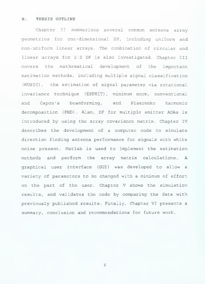
B. THESIS OUTLINE

Chapter II summarizes several common antenna array-

geometries for one-dimensional DF, including uniform and

non-uniform linear arrays. The combination of circular and

linear arrays for 2-D DF is also investigated. Chapter III

covers the .mathematical development of the important

estimation methods, including multiple signal classification

(MUSIC) , the estimation of signal parameter via rotational

invariance technique (ESPRIT) , minimum norm, conventional

and Capon's beamforming, and Pisarenko harmonic

decomposition (PHD) . Also, DF for multiple emitter AOAs is

introduced by using the array covariance matrix. Chapter IV

describes the development of a computer code to simulate

direction finding antenna performance for signals with white

noise present . Matlab is used to implement the estimation

methods and perform the array matrix calculations. A

graphical user interface (GUI) was developed to allow a

variety of parameters to be changed with a minimum of effort

on the part of the user. Chapter V shows the simulation

results, and validates the code by comparing the data with

previously published results. Finally, Chapter VI presents a

summary, conclusion and recommendations for future work.

II. ANTENNA ARRAYS

Antennas can be viewed as spatial filters; they enhance

signals in desired directions while simultaneously

suppressing signals in other directions. In a phased array,

the selectivity is achieved by phase shifting and then

superimposing the outputs of all elements [Ref . 1] . For a

passive array, the improvement in the signal-to-noise ratio

(SNR) is potentially equal to the number of elements. In an

array of identical elements, there are two related factors

that must be considered. The first is the geometrical

arrangement of the array (linear, circular, etc.) . Second is

the relative displacement between the elements, once the

element arrangement is set

.

A. UNIFORM LINEAR ARRAY

In most EW applications, it is desirable to use as few

elements as possible. For example, DF arrays on a ship are

linear arrays placed in the horizontal plane to measure the

azimuth angle. One linear array can theoretically cover up

to 180 degrees of azimuth angle, although it is often

limited to 120 degrees to avoid operating in the end-fire

mode [Ref. 1] . If the elevation angle is also of interest, a

linear array in the vertical direction has to be added. As

far as the AOA measurement is concerned, the two linear

arrays are usually treated separately.

Figure 3 shows a linear array with N elements indexed

from q-0,1,..., N-l along the x direction. Let us assume

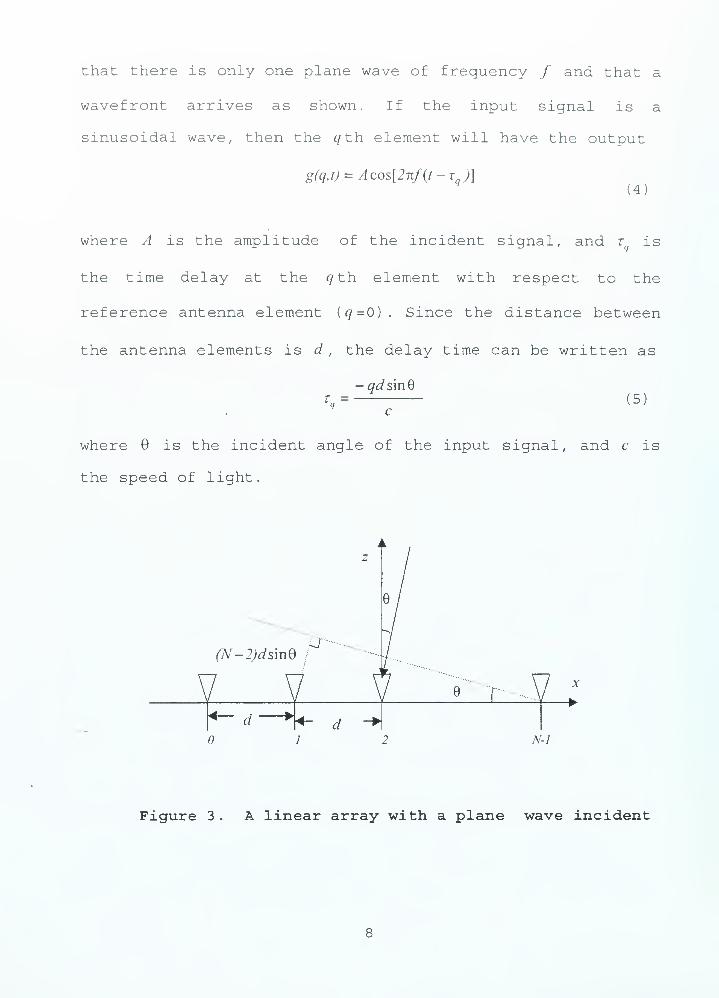
that there is only one plane wave of frequency / and that a

wavefront arrives as shown. If the input signal is a

sinusoidal wave, then the q th element will have the output

g(q,t) = Acos[2nf(t-t )]'(4)

where A is the amplitude of the incident signal, and t(

is

the time delay at the q th element with respect to the

reference antenna element (q=0) . Since the distance between

the antenna elements is d , the delay time can be written as

-qd sm§rq= (5)

c

where 9 is the incident angle of the input signal, and c is

the speed of light.

(N-2)d sinG

V V

cr

d—«-6 T £ X

N-l

Figure 3. A linear array with a plane wave incident

The minus sign in Eq. (5) is due to the fact that the

equiphase plane arrives at the q th element before it

reaches the reference element. Substituting Eq. (5) into Eq.

(4) gives

qdsinQg(q,t) = Acos[2M* + )] • ( 6

)

c

Let k be a unit vector pointing in the direction of the

wave propagation and x a unit vector along the direction of

array axis. Eq. (4) can be written as

g(q, t) = A cos(2/bi - 2nfqk x—) ( 7

)

c

r „ tz

where k • x = cos(—i- 0) = -sin0 .

2

If there are M signals, the output from the gth

antenna element is a superposition of all the received

signals

g(q,t) = Z An cos(2nfm t -Mf^s±)( 8 ,

m=l C

where /„, and km are the frequency and direction of the m th

signal . Often exponential form is used to express this

result as

g(q,t) =ZAm exp(j(2nfm t -2^qdkm -x

)} ( g

}

m=l C

In order to obtain digital data, the output is sampled at

discrete times and therefore the time t will be replaced by

integers n =0 , I , . . . , b -

1

, where b is the number of time

sample points. If we assume the frequencies of all signals

are the same, the factor e1 ' m ' can be suppressed, and a

standard phasor quantity results.

For an AOA measurement, the elements cannot be spaced

too far apart or an ambiguity will result [Ref . 1] . The

shortest distance between two antennas must be less than

half of the wavelength of the highest frequency in order to

fulfill the Nyquist theorem [Ref. 1] . Therefore, one must

sample the incident wavef ront twice per cycle

.

B. NON-UNIFORM LINEAR ARRAY (MINIMUM-REDUNDANCY)

By making use of a theorem by Caratheodory [Ref. 5] it

is shown that, 'for a given number of elements N , there

exits a distribution of element positions which results in

superior spatial spectrum estimators than the uniform linear

array. In addition to less hardware, certain nonuniform

arrays are capable of large dynamic range (spectral peak to

background level), lower sidelobes, and the relatively small

estimate bias values. A special type of nonuniform array is

the so-called minimum redundancy array (MRA) , in which

integer spacings of the base spacing occur only once. A MRA

is capable of resolving N(N-l)/2 multiple (simultaneous)

signals, whereas a conventional array can only resolve N-l .

Some minimum- redundancy array configurations are shown in

Table 1. A dot in column 3 represents an element and the

10

integers the number of base spacings between them. (The base

spacing is typically A./2 . )

A disadvantage of minimum-redundancy array is that its

resolution is not easily increased except by adding more

antennas and rearranging the array to the optimum

configuration for the new number of antennas. If there are

M signals, the output from the q th antenna element is

M Mmdakm ' X

})(10)

g(q,t)= I Am exp0(2nfm t

' m q m-))

where dq

is the distance between first antenna and the qth

antenna

.

Table 1 . Some minimum redundancy array configurations .

Number of elements. jV Array length Configuration3 3 .1.2.4 6 .1.3.2.5 9 .1.3.3.2.6 13 .1.5.3.2.2.7 17 .1.3.6.2.3.2.8 23 .1.3.6.6.2.3.2.9 29 .1.3.6.6.6.2.3.2.

10 36 .1.2.3.7.7.7.4.4.1

C. CIRCULAR ARRAY

A planar array can be used to measure both the azimuth

and elevation angles. These types of arrays occupy more

space than the linear array but they might be necessary for

some special aircraft and shipboard application. Planar

arrays include circular and rectangular (of which crossed

linear arrays can be considered a subset) . A circular

11

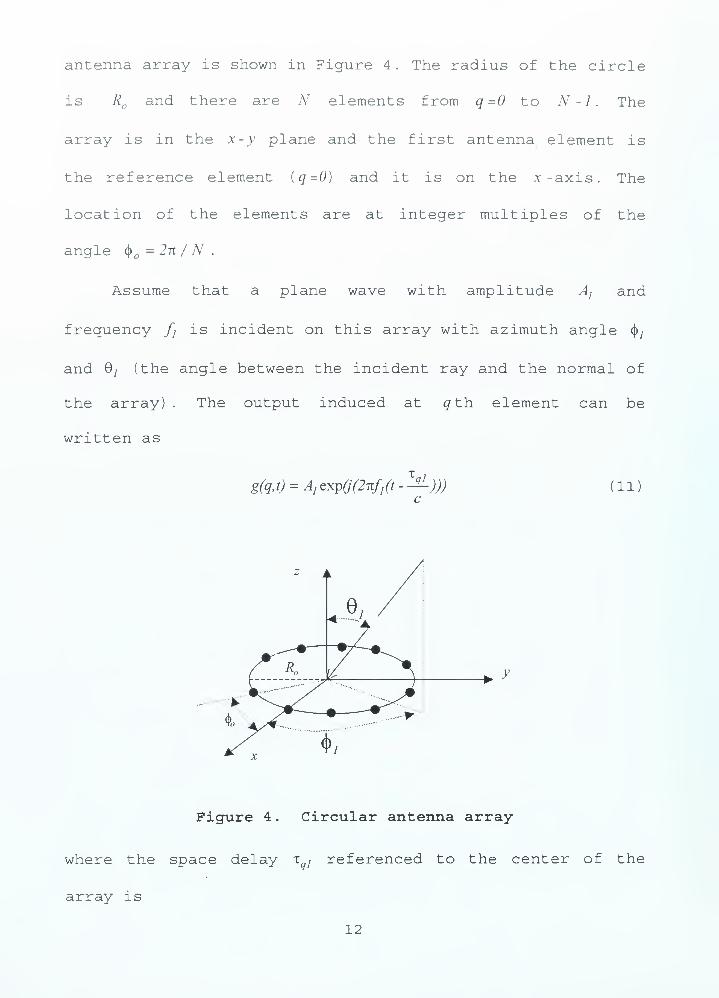
antenna array is shown in Figure 4 . The radius of the circle

is R and there are N elements from q =0 to N-l. The

array is in the x-y plane and the first antenna element is

the reference element iq=0) and it is on the x-axis. The

location of the elements are at integer multiples of the

angle § = 2n / N .

Assume that a plane wave with amplitude A}

and

frequency /;is incident on this array with azimuth angle <)),

and 6; (the angle between the incident ray and the normal of

the array) . The output induced at gth element can be

written as

gfqJJ^AjexpOVnfjft-^)))c

11)

Figure 4 . Circular antenna array

where the space delay x , referenced to the center of the

array is

12

xq i=-# sine, cos (f)^ . (12)

In this case, because the antenna locations are equally

spaced in azimuth, the angle <|)7can be written as

b qi=1$o-bi- (13)

Therefore

R sin Qj cos(—- -<j>

7 )

g(q,t) = A, exrtj2nf,(t + #))

2.7ZQR sin 6

;cos(—— -

<j>y )

= A, exp(j2n(f,t + —^)) . (14)

A.;

The incident direction of the input signal can be

represented by a unit vector k}in Cartesian coordinates as

kj = -(sinOj cos^/X + sinO/ s\n§ly + cosQ

]z) (15)

where x, y and £ are unit vectors in the Cartesian system.

The minus sign in front means the vector is pointing to the

origin. The position vector of the q th antenna element is

r where

rq=cos(q$ )x + sm(q$ )y (16)

so that

kj -rq=-smQ

1cos(q^ -^

l ) . (17)

Extending this to cover multiple signals ( m = 1,2,...,M ) gives

13

m R k -rg(q.t) = 14, exP02n(fm t - °

m q)) . (

i

8m = l K rm

The linear array can only provide azimuth angle

information because the corresponding propagation vector is

two-dimensional. The circular array can provide both azimuth

and elevation information since the corresponding

propagation vector is three-dimensional.

D. SPIRAL ARRAY

We examine a variation of the circular array, Eq. (18)

,

where the radial distances of the elements increase in steps

of R /(N-1). Therefore R = R q / N is the distance between

q th antenna element and the center point. The element

locations lie on an Archemedian spiral. In a circular array,

all antenna elements have the same Rq

. The output of qth

antenna element is as follows:

m R k r„

g(q,t)= ZAm exp02n(fj-q m q

)) . (19)

E. COMBINATION OF LINEAR AND CIRCULAR ARRAYS

A three dimensional array can be constructed by

combining planar and linear arrays. Figure 5 shows a

circular array in the x-y plane and a linear array along

the z axis. We examine the special case where the elements

of the circular array have § = 90 , which results in two

elements on the x and y axes equally spaced d from the

14

center. Let there be 3 the elements along the z axis, also

spaced d . Therefore, the array has seven elements, all

equally spaced.

y

Figure 5. There dimensional seven element array

The positions of the 3 elements of linear array are

given by the position vector

rh =(h-l)dz

where h = 1,2,3, so that

km -rh =-cos(Qm(h-l)d). (20)

If the array receives M signals, the output of h th

vertical antenna element of the linear array is

glinear(h,t) = % Am exp0(2nfj ^^))

m=l21)

15

Another four antenna elements comprise the planar array

which has an output of the form

m dkm r

Z circular (<l> = Z A„ QXp(j2n(fm t -— H-)) (22)

m=l km

where q=l,...,4, M is number of signals, and km -r is the

same as Eq. (18) . This array combines linear and circular

arrays to provide 2-D direction finding. From Eq. (21), it

is evident that the vertical array only provides elevation

angle information.

We have described the various array geometries. The

elements comprise the data acquisition system which samples

the incident signal wavefronts. The next step is to carry

out the estimation process. In the next chapter, we

introduce spectral -based algorithmic solutions to estimate

the AOA.

16

III. SPATIAL SPECTRUM ESTIMATION

Many different high-resolution approaches can be used

to estimate AOAs from digitized input data. In this chapter,

five high resolution methods will be discussed:

(1) Multiple Signal Classification (MUSIC) [Ref. 2.].

(2) Estimation of Signal Parameter via Rotational

invariance (ESPRIT) [Ref. 3]

.

(3) Capon's beamformer (Maximum Likelihood Method)

[Ref. 6]

.

(4) Pisarenko Harmonic Decomposition (PHD) [Ref. 7]

.

(5) Minimum norm [Ref.l].

All of these are cabable of (1) high resolution, (2)

estimating both azimuth and elevation AOA, and (3) handling

three-dimensional non-uniformly spaced array signals.

A. MUSIC

MUSIC is a technique used to determine the parameters

of multiple wavefronts arriving at an antenna array from

measurements made on the signals received at the individual

elements [Ref. 2 ]

.

The waveforms received at the N array elements are

linear combinations of the incident wavefronts from M

narrowband signals and noise. Thus, the multiple signal

classification approach begins with the following model for

characterizing the receive vector G as

17

G=AF+V (23)

where V a is noise vector. Expanding Eq. (23

S: a,{Q,) a,(Q2 )

a2 (Qj) a

2 (Q 2 )

>/" >/"

<*i®mY F2

v2

<*2<Pm)+

aN^M)_

-M_ 7n_

24

SN _

The size of each matrix is as follows:

G : vector of element outputs, N by 1

A : matrix of mode vectors, N by M

F : vector of signals, M by 1

V : noise vector, A^ by 1

The incident signals are represented in amplitude and

phase at some arbitrary reference point, for instance, the

origin of the coordinate system, by the complex vector F .

The elements of G and A are also complex in general. The

an (§m ) are functions of the signal arrival angles and the

array element locations. That is, an (Q m ) depends on the nth

array element, its position relative to the origin of the

coordinate system, and its response to a signal incident

from the direction of the mth source. The m th column of A

can be considered as a xmode' vector of responses to the

direction of arrival Q m of the m th signal. This N hy 1

mode vector will be denoted by a(Q) .

18

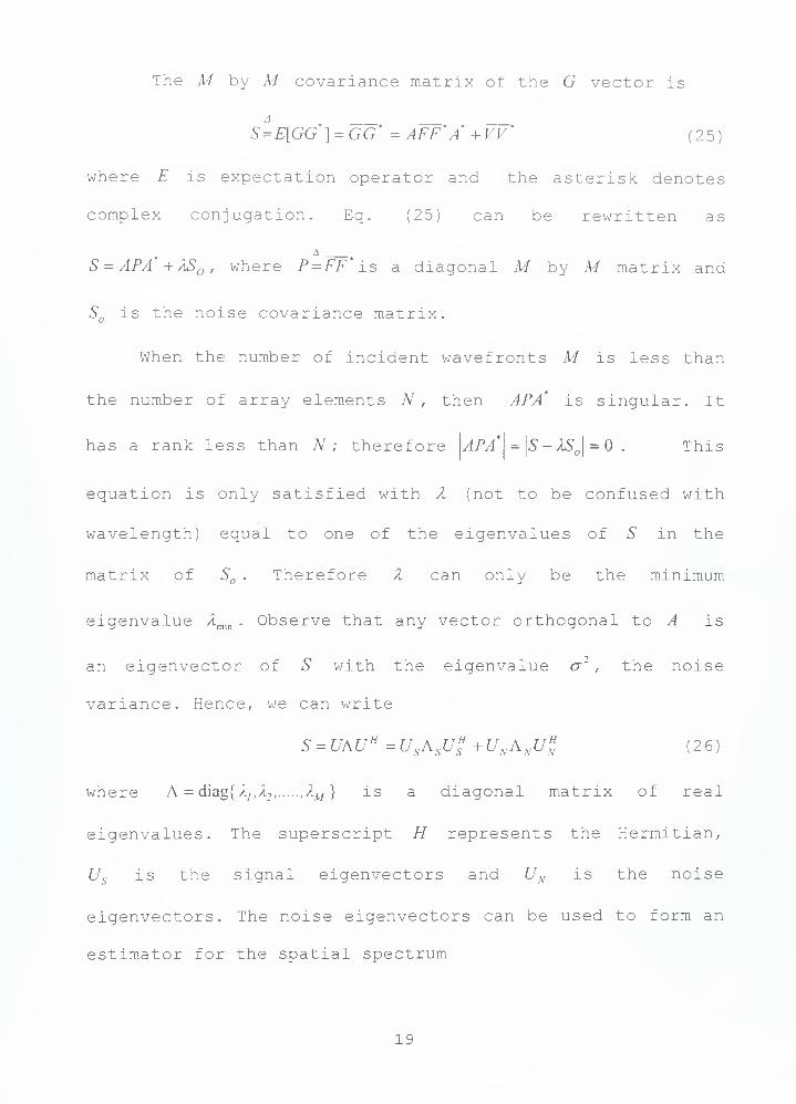
The M by M covariance matrix of the G vector is

S = E[GG*] = GG* =AFF*A* + VV' 25

where E is expectation operator and the asterisk denotes

complex conjugation. Eq. (25) can be rewritten as

A

S = APA' + AS() , where P = FF' is a diagonal M by M matrix and

S is the noise covariance matrix.

When the number of incident wavefronts M is less than

the number of array elements N , then APA' is singular. It

has a rank less than N ; therefore APA = LS-/LS 1 = This

equation is only satisfied with X (not to be confused with

wavelength) equal to one of the eigenvalues of S in the

matrix of S . Therefore A can only be the minimum

eigenvalue A.mm . Observe that any vector orthogonal to A is

an eigenvector of S with the eigenvalue a' , the noise

variance. Hence, we can write

S = UAUH =USA SU? +UNA NU% 26

where A = diag{ Xj,/.2 ,^-m) ^ s a diagonal matrix of real

eigenvalues. The superscript H represents the Hermitian,

Us is the signal eigenvectors and UN is the noise

eigenvectors. The noise eigenvectors can be used to form an

estimator for the spatial spectrum

19

PMu(*)=am»UNUJ!aQ)

27)

Although MUSIC is highly robust it requires characterization

of the array response and a spatial search through all

possible angles of arrival, G.

B. ESPRIT

ESPRIT [Ref. 3] eliminates the undesirable features of

MUSIC, but only under certain constraints. Assume that there

are N points of data (N antennas), which can be divided

into two groups, each consisting of N-l points. The first

group has an output signal x(t) = As(t) + n;(t) and the second

group y{t) = ABs(t) + n2 (t) , where A is a steering vector (not

related to A in Eq. (24)), s(t) denotes the baseband

waveforms, and B is a diagonal matrix

B =

vl

v2 .

vM

28

2tzwhere v

;

= exp(-y— <isin0() and d is antenna spacing. These data

A.

will be used to make two matrices by the covariance

approach.

20

Let Rxx be the auto-covariance matrix of x(t) and Rxy

the cross-covariance matrix of x(J) and y(t) . If there are M

signals then

Rxx=E[x(t)x*(t)]=ARA* +a 2I (29)

Rxy=E[x(t)y(t)]=ARB*A*+cr2J

](30)

where ^=[s(7)s (/)] is the signal covariance matrix under the

assumption of uncorrelated noise, / is the identity matrix

and Jj is an N by A^ matrix with ones along the first lower

diagonal off the major diagonal and zeros elsewhere. For a

pairwise matched array with doublets the cross covariance

matrix becomes

Rxy=ARB'A\ (31)

In the absence of coherent signals, eliminating cr~ , we

obtain

Cxx=Rxx-c2

/ = ARA*

C Xy=Rxy- cr2J

}

= ARB'A'

which gives

CXx- 7Cxy= AR{\-yB')A'. (32)

The singular values of Eq. (32) are given by the roots of

\l-yB'\ = 0. The desired singular values are

21

Vk:

= vk , k=l,2, . . ,M.

To find the angles we note that for a uniform linear

array, the angles of the eigenvalues are equal to 2^7rsinG so

that

8* =sirT/ (^-) (33)

where S kis obtained from y k

= exp(y9A.)

. Thus, the direction

of arrival can be obtained without a search technique. In

this respect computation and storage costs are reduced

considerably.

C . BEAMFORMING

1 . Conventional Beamformer

The first attempt to automatically localize signal

sources using antenna arrays was through beamforming

techniques. The idea is to steer the array beam in one

direction at a time and measure the output power. The

steering locations which result in maximum power yield the

DOA estimates. The array response is steered by forming a

linear combination of the antenna outputs

y(t) = £w*gi (t) = WHG(t) (34)

1=1

where g t{t) is the output of the /th element, and w,-(0 the

corresponding complex weight factor. The output power for b

time samples is

22

P(W) = -Y\y{t)\ =-tw HG{t)G

H{t)W = WHRW (35)

b t=o b 1=0

where R is the signal covariance matrix defined previously.

The conventional beamformer is a natural extension of

classical Fourier-based spectral analysis to antenna array

processing. Suppose we wish to maximize the output power

from a certain direction 9 , given a signal s(t) emanating

from direction . A measurement at the element output is

corrupted by additive noise n(t) and written as

g.(t) = a!(9)s

l(t) + n

j(t) . The problem of maximizing the output

power is formulated as,

max[E{w HG(t)GH (t)w} ] = max[WHE^}(t)G

H(k

t)\v]

= maxlE\s(t)\2\w

Ha(Q)\

2

+ a2\W\

2\

where the assumption of spatially white noise is used. The

resulting solution is

1/(6)0(6)

The above weight vector can be interpreted as a spatial

filter, which has been matched to the impinging signal.

Using the weighting vector, the classical spatial

spectrum estimator is

PBF (Q) = aH(Q)Ra(Q) (38)

where R is the signal covariance matrix.

23

For a uniform linear array of isotropic sensors, the

steering vector is

a(Q) = 1 e** e20

. . . e>^1J

*f 39)

where <t> = -kdsinQ , N is number of elements and T denotes

transpose. The standard beamwidth [Ref. 6] for a uniform

2tzlinear array is — , so sources whose angles are closer than

N

this beamwidth will not be resolved by the conventional

beamformer, regardless of the available data quality.

2 . Capon' s Beamformer

In an attempt to alleviate the limitations of the

conventional beamformer, such as its resolving power of two

sources spaced closer than a beamwidth, an improved method

was proposed by Capon [Ref. 7] . The optimization problem was

posed as min{P(W)} , subject to WHa(Q) = 1 . Hence, Capon's

beamformer (also known as the minimum variance

distorsionless response filter) attempts to minimize the

power contributed by noise and any signals coming from

directions other than 9, while maintaining a fixed gain in

the look direction G . The optimal W can be found using

methods such as the technique of Lagrange multipliers [Ref.

6] , resulting in

WCAP - /""(?>. (40)

24

Using the above weight vector, we can find the following

spatial spectrum

pcap(Q) = —rf; • (41)

The power minimization can also be interpreted as

sacrificing some noise suppression capability for more

focused rejection in the directions where there are other

sources present. The spectral leakage from closely spaced

sources is therefore reduced, though the resolution

capability of the Capon beamformer is still dependent upon

the array aperture and on the signal-to-noise ratio though

R .

D. PHD

The PHD is based on the use of a noise subspace eigen-

vector to estimate the incident angle and assumes that the

process consists of M complex signals in additive complex

white noise. It derives the angle of the signals, their

powers and the white noise variance from the known

autocorrelation sequence. This algorithm accounts for the

conjugate symmetry of the eigenvector. This method is based

on an estimation of angles by using the orthogonality

property between the signal vectors and vectors in the noise

subspace. The minimum eigenvector is orthogonal to the

signal vectors, thus we have

aiH(Q)uN =0, i = l,2,...,M . (42)

25

Once the minimum eigenvector uN is found the from UN in Eq.

(26) , the angles of the signals may be determined by

factoring the eigenfilter polynomial [Ref. 7]. The roots are

guaranteed to be on the unit circle. The a(Q) is a steering

vector that will be zero whenever G = G, , one of the angles

of the signals. This leads to the angle estimator function

1

PpHD^)~II

a"(Q)uf

7 ' 43)

MINIMUM NORM METHOD

This method and the MUSIC method are somewhat alike.

The basic idea is to find a vector D that is a linear

combination of eigenvectors in the noise subspace. This

vector D can be written as

Z) = [8 5; . . . 8^]T = [l 5 ;

. . . d N f (44)

where the superscript T signifies the transpose and TV the

number of antenna elements. In this equation d is assigned

to be unity. The square of the norm of Eq. (44) is

8 = Z 8?i=0

where M is the number of sources. The minimum norm method

minimizes this quantity and hence the name. The procedure is

as follows:

26

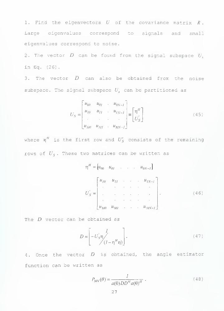
1. Find the eigenvectors U of the covariance matrix R.

Large eigenvalues correspond to signals and small

eigenvalues correspond to noise.

2. The vector D can be found from the signal subspace Us

in Eq. (26) .

3. The vector D can also be obtained from the noise

subspace. The signal subspace U can be partitioned as

uoo U0l U0N-1

us =U 10 Ujj U1N-1 =

_UM0 UM1 UMN-1_

45)

where r\H

is the first row and U's consists of the remaining

rows of Us . These two matrices can be written as

T]H = [u00 U0] U0N-l\

Us =

Ulf)

Ujj 1 1N-I

UM0 UM1 UMN~1

(46:

The D vector can be obtained as

D = -Ust\,

V-T\H

T\)

47

4. Once the vector D is obtained, the angle estimator

function can be written as

/

Pmn(8) =a(Q)DDHa(Q)H

27

48)

So far several high resolution techniques have been

applied to the problem of resolving the directions of

arrival of incoming signals. From a statistical point of

view, the signals arriving at the array can be regarded as

random, and thus the signals and noise are uncorrelated. In

the next chapter, we implement these methods based on finite

observations

.

28

IV. IMPLEMENTATION AND COMPUTER CODES

A. PARAMETRIC DATA MODEL AND FLOWCHART

The AOA estimation methods described in Chapter III

were implemented in a computer code. Output data were

gathered for a variety of arrays and signals, and a

performance comparison made. This chapter describes the

structure and operation of the computer simulation, which is

written in Mat lab. The approach is model -based in the sense

that it relies on certain assumptions made on the

observation data. Since the natural causes responsible for

signals and noise are often unrelated, it is customary to

assume that the signals and noise are uncorrelated with each

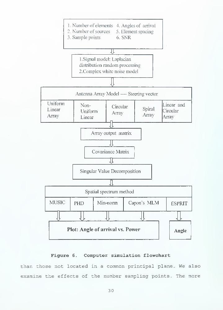
other. Figure 6 shows the flowchart of the computer program,

with the main steps described in the following sections.

1 . Input Parameters

For an antenna array with N elements, the size of

correlation matrix (correlation between /th and j th

element) is N by N . In this case, the maximum number of

sources that can be detected cannot exceed (iV-1) . Because

the effectiveness of these spatial spectrum methods are a

function of signal-to-noise (SNR) ratio, we evaluate the

performances of each antenna array by changing SNR at the

input. Also, we must consider the spatial resolution

capability of each estimation method when applied to each

array geometry. For example, test signals that have the same

azimuth or elevation angle are generally harder to resolve

29

1

.

Number of elements 4. Angles of arrival

2. Number of sources 5. Element spacing

3. Sample points 6. SNR

IT1. Signal model: Laplacian

distribution random processing

2.Complex white noise model

IAntenna Array Model— Steering vector

Uniform

Linear

Array

Non-

Uniform

Linear

Circular

Array

£

Spiral

Array

Linear and

Circular

Array

Array output matrix

iz

Covariance Matrix

TSingular Value Decomposition

JLSpatial spectrum method

MUSIC PHD Min-norm Capon's MLM ESPRIT

1Z lz Iz 2Z

Plot: Angle of arrival vs. Power

±z.

Angle

Figure 6 . Computer simulation flowchart

than those not located in a common principal plane. We also

examine the effects of the number sampling points. The more

30

sampling points, the more accurate the AOA estimate but it

occurs at the expense of increased processing time.

Generally the antenna spacing must be less than 0.5 A in

order to avoid the ambiguity problem.

2 . Signal and Noise Models

In practice, the white noise and signals are modeled as

a independent and identically distributed random processes.

That means we interpret the received signals as the sample

of some waveform at certain specified instants of time, and

is referred to as a realization of a discrete time random

process. In all cases the signals that arrive can be

regarded as random, we assume that signals s(n) are

Laplacian probability distributed processes. Because all

arrays are not diverse in polarization (i.e., they have all

elements identically polarized) , we assume that the

frequency and polarization of all received signals are the

same. Multi-path and re-radiators in the vicinity of

receiving site which may have a mutual coherence are not

considered.

The signal and white noise generation process are

described by the following Matlab pseudo-code:

u{ri) = rand(rc) - 0.5

s(n ) = -(u(n)) * log(l - 2*|u(n) |)

* A

Np

w(n) = —^v(n)V2

v(n) = randn(«) + j* randn(rc) (49)

31

where n =0, 1 , . . . , 4095, A is the signal amplitude, N the

peak amplitude of white noise and the noise v(n) is a

complex Gaussian random variable with both the real and

imaginary parts having a variance equal to 1. The Matlab

functions rand and randn can be used to generate Gaussian

distributed random values. The voltage ratio A/N

determines the SNR; in dB it is 2 log]0(A/ N ) . For

convenience we let A =1 so that

Np=\0-sm/2°

. (50)

3 . Antenna Array Model

Based on the discussion in Chapter II the steering

matrices for five array geometries can be determined. The

steering matrix for the uniform linear array takes the form

1 ...i

AQ) =

exp(j2ii(N - l)d sin(J) 7 ) exp(j2n(N - l)d sin (j)M )

51)

where N is the number of antenna elements, M is the

number of sources and §M is the AOA of the Mth source,

- ft/ < rh < ft/

The steering matrix for a the non-uniform linear array

is

32

AQ) =

Qxp(j2ndx _]S'm§i) Qxp(j2ndiW_,sm^M )

52

where dl

is the spacing between the reference element and

the (/+l)th antenna. For a minimum redundancy array, the dt

are specified in Table 1.

The steering matrix for circular array is

exp(J2nR cos(-(f)/)sinO

/) • • • exp(j2nR cos(-(j)

/)sinG

A/ )

,4(9, 40

Qxp(j2nR cosC^^sinG/) exp(j2nR cos((|) NM ) sin M )

53

where <j>„m - n§ -(j)m , Qm is the elevation angle of mth source,

(J)m is the azimuth angle of mth source and R is the

radius of the circle. For the present analysis it is

assumed that R is equal to 0.5 A, <tym < 2n, and < m <^ .

The steering matrix for the spiral array is

Qxp(j2nRj cos(-$I)smQ

! ) • • • exp(j2nR; cos(-(j);)sin0 A/ )

A(Q,$) =

Qxp(j2nRN cos((j) N1 ) sin l ) exp(./27t# v cos(<|)^ ) sin M )

54

where Rn is the distance between nth antenna element and

center point. In our model, the maximum Rn is 0.5/1.

33

The steering matrix for the combination linear and

circular array can be partitioned into sub-matrices

associated with the linear and circular parts of the array

^(0,*)

1

Qxp(j2nds'mQl )

exp(j4nd sinO ,)

exp(j2nd cos(-§j)smQ j)

exp(j2nd cos((j) v/ ) sin 9 ,

)

1

exp(j2nd smQM )

exp(j4nd s'mQM )

exp(j2nd cos(-<bM )smQM )

z*p(j2nd cos(<{>NM ) sin GM )

55

where d is . 4 A . The first three rows in Eq . (55) are for

the linear array elements. For these terms there is no

dependence on arrival azimuth angle.

4. Correlation Matrix and Spatial Spectrum Methods

The output of the array can be calculated by using the

signal, noise, and antenna models in Eq. (24) . First the

Matlab function is used to find the singular value

decomposition. The result is substituted into the various

algorithms (Eq. (27), (41), (43), or (48)) with the

appropriate antenna array steering matrix (Eq. (51) , (52) ,

(53), (54), or (55)). The outputs for MUSIC, PHD, minimum

norm and Capon's beamformer are angle of arrival vs. power.

The power must be computed at every angle. We must steer the

antenna array in all azimuth directions (0 to 360 degrees)

and elevation direction (0 to 90 degrees) in order to find

the AOAs . The output of ESPRIT is the direction of arrival

34

which can be obtained without a search. This method has only-

been applied to a uniform linear array.

B. THE IMPLEMENTATION OF ARRAY MATRIX DECOMPOSITION

The signal measured at the output of any element in the

array differs from the signal actually received by an amount

attributed to noise. Thus, we have an observed signal, which

for each element of the array, consists of the actual

received signal plus narrow-band noise. Calculations used

6=4096 time sample points for each antenna element, so the

size of received signal matrix is N by 4096, where N is

the number of elements. The size of signal -in-space matrix

is M by 4096, where M is the number of sources. The

observed signal matrix is equal to the received signal

matrix times the propagation delay matrix. The observed

signal matrix is the antenna output matrix G , from which we

find the covariance matrix of the observed signal matrix

defined by

R = E [G* G T] .

The covariance matrix R has two important special

properties. First, it is Hermitian, that is, it is equal to

the conjugate transpose of itself. Second, it is positive

semi-definite if element noise is present. Thus, for

computer coding purposes

R = E [G* G T]= E [G G H] . (56)

35

The size of R matrix is N by N . The Matlab function SVD

is used for singular value decomposition. It has the form

[U, S, U] = SVD(R)

where R = USU H(Eq. (26)). The eigenvector U is an N by N

orthogonal signal and noise subspace matrix, and S is an

TV by N diagonal matrix. The singular value decomposition

is accurately computed by this function. The columns of U

are the eigenvectors of RR , and the entries along the

diagonal of S are the correspondingly ordered nonnegative

square roots of the eigenvalues of R R , which are also the

eigenvalues of RR . The numbers in S are the singular

values of the matrix R , which is determined by the number

of sources. After calculation of U and S , they are

substituted into the spectral estimators in Eqs . (27),

(43), and (48) to determine the AOAs

.

The MUSIC and PHD methods make use of the noise

subspace matrix; the minimum norm method uses the signal

subspace matrix. Capon's beamformer does not use the

singular value decomposition of the covariance matrix. For

2-D direction finding, it takes a significant amount of CPU

time to search space in order to find the AOAs. The default

search range in azimuth angle is 90 degrees.

36

c. GRAPHICAL USER INTERFACE

To compare the relative performance of the various

arrays and algorithms, the simulation must be run for many-

cases. A graphical user interface (GUI) was developed to

vary the input parameters, as shown in Figure 7. Also

included is an on-line help feature. The help button

provides brief explanations of the input parameters. The GUI

provides default values to demonstrate the angular

resolution of MUSIC for a uniform linear array and a minimum

redundancy array with different signal-to-noise ratios.

antenna number: 7 spacing: f^"source number:

Signal to Noise Ratio(dB):

CLOCK

CLOSE HELPsample points: pioiT

1-D DIRECTION FINDING -90 ...90

** 'y ** * * i i i>- >

Unifiorm and Non-uniform Linear Array

2-D DIRECTION FINDING: EL

angle:0...90deg. AZ angle: 0.

AZ angle: j 16 | 22 | 28 | 34

MUSIC-resolution- MOVIE

Linear Array with ESPRIT

EL angle: | 10 j 15 j 20 [ 25

2-D DIRECTIONFINDING CIRCULARARRAY

Antenna Geometry

Uniform Linear Array

Non-uniform linear array

2-D DF Array

2-D DIRECTIONFINDING SPIRAL ARRAY

2-D DFLINEAR+CIRCDLARARRAYLA-spacing: g.4

LA-ant No: ~3~

Antenna Pattern

Linear*circular array

Circular array

Figure 7 . Graphic user interface

In the next chapter, we use this GUI to present a

performance comparison of superresolution spectral

37

algorithms for elevating and analyzing their effectiveness

in several antenna and emitter geometries.

38

V. SIMULATION RESULTS AND ANALYSIS

In this chapter the results of the computer simulation

are presented. The performances of the various algorithms

with different array and emitter geometries are examined.

Computer simulations were run for the conditions of: (1) two

closely spaced AOAs for testing azimuth and elevation

angular resolution, (2) various levels of additive white

noise, (3) multiple signal sources, and (4) changes in the

antenna element spacing.

By comparing the test results, we can determine which

combination of array and algorithm operates best under the

given set of conditions. The power spectra are plotted as

surfaces. For all cases, the z -axis represents magnitude of

the power, the x-axis represents as azimuth angle and the

;y-axis the elevation angle. The majority of the cases use 7

antenna elements; the exceptions are Figures 3 5 and 3 7

which are for 10 elements.

A. ANGULAR RESOLUTION OF ONE -DIMENSIONAL DF

Initial simulations were run to determine the

comparative performance of algorithms in resolving closely

spaced AOAs. The signals were assumed to be of equal

frequency, polarization and mutually incoherent.

Simulations were run for two signals with angles of

arrival of 15 and 18 degrees; the corresponding spectral

estimates are shown in Figure 8 . The rows correspond to

spectra estimates for the PHD, MUSIC, minimum norm and

Capon's beamformer algorithms, and the columns correspond to

39

the uniform array (left) and non-uniform linear array

(right) . From this figure, we can see that the non-uniform

array can achieve better angular resolution. All algorithms

except the Capon's beamformer provide sharp distinguishable

peaks, but MUSIC has a smoother spectrum (the separation of

the peaks is not as pronounced) . Figure 9 shows an

interference simulation for 6 sources. The non-uniform

(minimum redundancy) array provides better dynamic range for

all algorithms.

B. TWO-DIMENSIONAL DIRECTION FINDING

1. Azimuth Angular Resolution

A range of SNRs were simulated. Figures 10, 11, and 12

show the results for a high SNR (=25 dB) , at an elevation

angle of 15 degrees and AAZ=5 degrees. The MUSIC, PHD and

min-norm methods have similar results for all three 2-D

array geometries except the Capon's beamformer. However,

when the SNR is lower (15 dB) , the circular array performs

better, as indicated by a comparison of Figures 13, 14, and

15. Even though two peaks exist, there is no notch between

them and therefore it may be difficult to correctly resolve

the two spectral peaks. Figures 16, 17, and 18 show the

results for SNR=3 dB, and two sources at the same elevation

angle but separated in azimuth ( AAZ = 3 degrees) . All arrays

can resolve the two peaks. However, for the lower SNR level

case, the circular array is generally superior.

40

Uniform linear array

m PHD |T3

(D-50 A

1Q. .mn—^^

Non-unifonn linear array

MUSIC

1

\

-50-100 -50 50

AOA(degree)

-50-100 -50

AOA(degree)

100

100

100

100

Figure 8. Comparison of uniform (left) and non-uniform (right)

linear arrays , 2 sources , 7 elements , separation angle 3 degrees(15° and 18°) . SNR=25 dB

Uniform linear array

-100 -50 50

AOA(degree)

Non-uniform linear array

100

ma

100

CD

100

-50

-100-100 -50

-50

-100-100 -50

50

100

MUSIC

L."

100

Mini-norm

100

100

-50 50

AOA(degree)

100

Figure 9. Unifrom (left) and non-uniform (right) linear arrays,

SNR=25 dB, 7 antennas, 6 sources: 15°, 25°, 35°, 45°, 55°, and 65°

41

MUSIC PHD

50

EL(deg)

50

AZ(deg)

Mini-norm

EL(deg) AZ(deg)

Capon MLM

100

EL(deg) AZ(deg) EL(deg) AZ(deg)

Figure 10. Linear+circular array, SNR=25 dB, 2 sources at(16°. 15°) and (21°, 15°) . 7 elements

MUSIC

EL(deg) AZ(deg)

Mini-norm

PHD

~ 60-QQ Z.3 40-

1 20-

S. o.

-20 J

EL(deg) AZ(deg)

Capon MLM

EL(deg) AZ(deg)

10050

AZ(deg)

Figure 11. Circular array, SNR=25 dB, 2 sources at (16°, 15°)

and (21°. 15°) . 7 elements42

MUSIC PHD

EL(deg) AZ(deg)

Mini-norm

50 50

EL(deg) AZ(deg)

Capon MLM

50

AZ(deg)

50

AZ(deg)

Figure 12. Spiral array, SNR=25 dB, 2 sources at (16°, 15°) and(21°, 15°) , 7 elements

MUSIC PHD

60 i

m 40--a

|f 20-

1 o.

-20-

~ 60-CD .„% 40-

1 20-°a. u

-20 J

EL(deg) AZ(deg)

Mini-norm

EL(deg) AZ(deg)

Capon MLM



and (21°, 15°), 7 elements

43

MUSIC PHD

EL(deg) AZ(deg)

Mini-norm

EL(deg) AZ(deg)

Capon MLM

EL(deg) AZ(deg)

10050

AZ(deg)

Figure 14. Linear+circular array, SNR=15 dB, 2 sources at(16°, 15°) and (21°,16°)

/ 7 elements

MUSIC PHD_..••'

60-

m 40 •

f 20-

1 0-

-20 -

•• ^im

50^ -"~"~50

E L(deg) a:^(deg)

norm

CD"C3

EL(deg) AZ(deg)

Capon MLM

EL(deg) AZ(deg)

10050

AZ(deg)

Figure 15. Spiral array, SNR=15 dB, 2 sources at (16°, 15°)


44

MUSIC PHD

EL(deg) AZ(deg)

Mini-norm

EL(deg) AZ(deg)

Capon MLM



(19°, 15°) , 7 elementsand

MUSIC

EL(deg) AZ(deg)

Mini-norm

EL(deg) AZ(deg)

PHD

EL(deg) AZ(deg)

Capon MLM

EL(deg) AZ(deg)

Figure 17. Linear+circular array, SNR=30 dB, 2 sources at(16°,15°) and (19°. 15°). 7 elements

45

MUSIC PHD

50

Mini-norm

30j

•"'.'.'/:'"'.'.[ "•!!' ••..

m 60j? 40- .;..--i

i/^^| 20-

§. o. ^^^^H ^^_ 'Lj^^CncSkVBP^^^^^-20 J

50

80 h

m 60-

?- 40-

| 20-

g. 0-

-20 J

50 50

EL(deg) AZ(deg)

Capon MLM


Figure 18. Spiral array, SNR=30 , 2 sources at (16°, 15°) and(19°, 15°) , 7 elements

60

I 20 r

60 •

od 40

I 20

-20

MUSIC

EL(deg)Mini-norm

60 80

20 40 60 80

EL(deg)

PHD80

60 r

m /in-o 40

A: :....

50

EL(deg)

100

Figure 19. Circular array, SNR=25, 2 sources at (16°, 15°) and(16°, 18°) , 7 elements

46

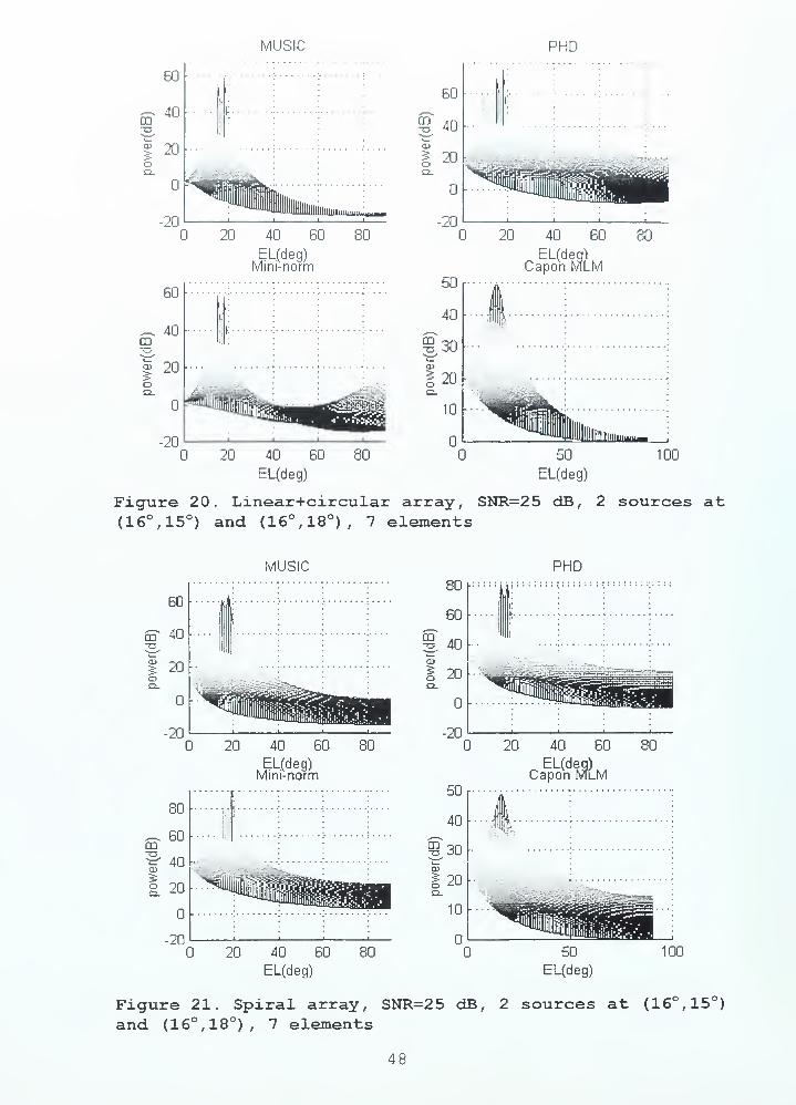
2 . Elevation Angular Resolution

Simulations were run for the two signal case with

angles of arrival at 18 and 15 degrees in elevation and 16

degrees in azimuth. For the SNR equal to 25 dB, the

corresponding spectral estimates are shown in Figures 19,

20, and 21. The results for the circular and linear+circular

arrays are almost the same, but the spiral array cannot

correctly resolves the peaks. For a 15 dB SNR the data,

which is shown in Figures 22 and 23, indicate that all

algorithms, except Capon's beamformer, correctly resolve the

two spectral peaks with a circular array. Only two

algorithms can resolve the peaks for the circular array, so

the elevation angular resolution of the linear+circular

array appears to be better for this scenario.

3. Multiple Signal Sources

Multiple signal simulations are shown in Figures 24,

25, and 26. There are four signals arriving at azimuth and

elevation angles of (10°, 20°), (55°, 15°)

, (30°, 16°) , and (45°, 25°)

with equal amplitudes. The circular antenna array and

linear+circular array can resolve the four peaks but the

circular array has more sidelobes. Only the MUSIC algorithm

correctly resolves the signal sources for the spiral array.

In this scenario the linear+circular array is best.

47

MUSIC PHD

LLJ

in

OQ.

LI I

41

20

-20I

60

40

20

-20

1TJ

ili

:::

20 40 BO

EL.(deg)Mini-norm

CD

i

—

Hi

oa.

60

40

20

-20

50

40

30

20

10

,

:

I-

Stf&5MftfcmJ^i^i^j^^Bn

i i . i

20 40 60 80

EL(deg)Capon MLM

20 40 60

EL(deg)

80

Figure 20. Linear+circular array, SNR=25 dB, 2 sources at(16°

/15°) and (16°, 18°), 7 elements

MUSIC PHD

60

S 40

I 20

-2020 40 60

ELfdeg)Mini-norm

80

_ 60CD

^401 20

: : : :

•

Ill

1 :

:

"

» -ZAindaeMaa** '

t

20 40 60 80

EL(deg)

Figure 21. Spiral array, SNR=25 dB, 2 sources at (16°, 15°)


48

MUSIC PHD

40

LLJ

5 20

o

-20

20 40 60 80

EL(deg)Mini-norm

20 40 60 80

EL(deg)apon MLM

BO

~ 40oo—5 20

-20

20 40 60

EL(deg)

80



MUSIC PHD

60 r

£T40

| 20b

-20

20 40 60 80

EUfdeg)Mini-norm

EL(deg)Capon MLM

60

m 40 •

-a

I 20o

-2020 40 60

EL(deg)

80 100

Figure 23. Linear+circular array, SNR=15 dB, 2 sources at

(16°, 15°) and (16°, 18°), 7 elements49

Mi i:-";ii PHD

60-

S 40-

powen

rj

isj

CD

CD

CD

50

"S*

50

EL(deg) AZ(deg)

Mini-norm

50

AZ(deg)

Capon MLM

50

CD[^M

50

AZ(deg)

100

Figure 24. Linear+circular array, SNR=25 dB, 7 elements, 4

sources at (10°, 20°), (55°, 15°)

, (30°, 60°) , and (45°, 25°)

MUSIC

50

AZ(deg)

Mini-norm

PHD

EL(deg) AZ(deg)

Capon MLM

EL(deg) AZ(deg)

50

AZ(deg)

100

Figure 25. Circular array, SNR=25 dB, 7 elements, 4 sources at(10°, 20°)

,(55°, 15°)

,(30°, 60°) , and (45°, 25°)

50

MUSIC PHD

80 a

EL(deg) AZ(deg)

Mini-norm

50

AZ(deg)

.•'..!'

•

'

5050

EL(deg) AZ(deg)

Capon MLM

50

AZ(deg)

Figure 26. Spiral circular array, SNR=25 dB, 7 elements, 4

sources at (10°, 20°),(55°, 15°)

,(30°, 60°) , and (45°, 25°)

MUSIC PHD

50

AZ(deg)

Mini-norm

50

AZ(deg)

50 50

EL(deg) AZ(deg)

Capon MLM

50

AZ(deg)

Figure 27. Circular array, SNR=15 dB, 7 elements, 2 sources

at (16°, 15°), and (16°, 20°)

51

4. Comparison of Azimuth and Elevation Angular

Resolution

The estimation methods and arrays were compared for

two emitters with a 5 degree separation. Figures 27, 28, and

29 are for SNR=15 dB and AEL=5 degrees; Figures 13, 14, and

15 for SNR=25 dB,' AAZ=5 degrees. We see that the elevation

angular resolution is better than the azimuth angular

resolution since the sidelobes in azimuth are higher than

the sidelobes in elevation for all three array-

configurations. Even at lower SNRs , all three arrays

employing the MUSIC method can distinguish the two sources

in elevation.

5. Improvement of Angular Resolution of Two-dimensional

DF

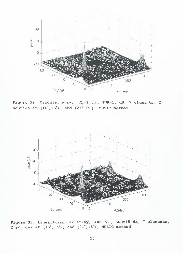
Next we investigate changing the radius of the circular

array to 1.5 wavelengths. The results are shown in Figures

30 and 31. Comparing Figures 13 and 14 with Figures 30 and

31 (SNR=15 dB, AAZ = 5 degrees) , the angular resolution is

better with the larger radius as expected. Larger spacing

may be susceptible to ambiguities. From Figures 32 and 33,

where the range of azimuth angles is from to 360 degrees,

it is evident that there is no serious ambiguity problem.

Thus, we can improve the angular resolution by . changing the

antenna spacing.

52

MUSIC PHD

m 40-t3*=• 20-a>

1 o.a.

-20 ^

EL(dgg) AZ(deg)

Mini-norm

50

AZ(deg)

50 50

EL(deg) AZ(deg)

Capon MLM

50

AZ(deg)


sources at (16°, 15°), and (16°, 20°)

MUSIC

50

AZ(deg)

Mini-norm

50

AZ(deg)

PHD

60 -I

50 50

EL(deg) AZ(deg)

Capon MLM

Figure 29. Spiral array, SNR=15 dB, 7 elements, 2 sources

at (16°, 15°), and (16°, 20°)

53

The circular array has a smoother spectrum and less

spikes than linear+circular array, since the spacing of

linear array part is larger than o . 5 A, . From these

simulation results, we conclude that the larger antenna

spacing will enhance angular resolution at the expense of

more ripples on the spectrum. We can suppress the sidelobes

and enhance resolution by increasing the number of elements

in the x - y plane and increasing the radius of circle and

then adding a linear part on z -axis with a spacing less

than 0.5/1.

Two elevation cases are considered. For a large

elevation angle (80 degrees) , there are four signals

arriving at azimuth and elevation angles of (10°, 80°),

(90°, 80°) , (180°, 80°), (270°, 80°) , with a SNR=15 dB . The

simulations are shown in Figure 34 for the circular array (7

elements, Rn=1.5A), and in Figure 35 for the

circular+linear array (3 elements, d =0.4/1 on z -axis) . In

both cases the sidelobes increase in the elevation

direction, but Figure 35 shows lower sidelobes. From these

results we conclude that the elevation angular resolution is

worse when the elevation angle is large. This is a well

known result that is associated with the increase in

beamwidth that occurs with array scanning [Ref . 9]

.

For small elevation angles (5 degrees) , there are four

sources arriving at azimuth and elevation angles of

(10°, 5°), (90°, 5°) , (180°, 5°)

, (270°, 5°) , and a SNR=15 dB . The

54

simulations are shown in Figure 36 for the circular array (7

elements, Rn =1.5A), and in Figure 3 7 for the

circular+linear array (3 elements, d=0.4A). Figure 37

shows lower sidelobes in the plane of the sources. These

sidelobes expand in the azimuth direction, implying that the

azimuth angular resolution is worse when the elevation angle

is small. This case is close to a broadside condition for

the linear array and, consequently, the resolution ability

is essentially that of the linear array. Thus the resolving

ability has been improved at low elevation by adding a

linear array part (3 elements on the z axis)

.

Based on the results of the computer simulations and

performance comparisons, we present some conclusions and

recommendations in the next chapter.

55

MUSIC PHD

EL(deg) AZ(deg)

Mm i- norm

U 1 ,

m 40-

» 20-^ no •

Q.

-20 J

EL(deg) AZ(deg)

Capon MLM

EL(deg) AZ(deg)

50

AZ(deg)

100

Figure 30. Circular array, Rn=1.5/l r SNR=15 dB, 7 elements, 2

sources at (16°, 15°), and (21°, 15°)

MUSIC PHD

EL(deg) AZ(deg)

Mini-norm

m 40

EL(deg) AZ(deg)

Capon MLM

EL(deg) AZ(deg)

1 00

Figure 31. linear+circular array, d =1.5/1, SNR=15 dB, 7 elements,

2 sources at (16°, 15°), and (21°, 15°)

56

EL(deg) AZ(deg)

Figure 32. Circular array, R =1.5A,, SNR=15 dB, 7 elements, 2

sources at (16°, 15°), and (21°, 15°), MUSIC method

EL(deg) AZ(deg)

Figure 33. Linear+circular array, d =1.5 A, SNR=15 dB, 7 elements,

2 sources at (16°, 15°), and (21°, 15°), MUSIC method

57

EL(deg) AZ(deg)


,(90°, 80°)

, (180°, 80°) , and (270°, 80°) , MUSIC method

EL(deg) AZ(deg)

Figure 35. Linear+circular array, SNR=15 dB, 10 elements , 4 sourcesat (10°, 80°)

,(90°, 80°)

, (180°, 80°) , and (270°, 80°), MUSIC method

EL(deg) AZ(deg)


,(90°, 5°)

,(180°, 5°) , and (270°, 5°), MUSIC method

EL(deg) 111

AZ(deg)


sources at(10°,5°) ,(90°, 5°)

,(180°, 5°)

,(270°, 5°)

, MUSIC method

59

VI. CONCLUSIONS

Over the past few decades superresolution techniques

have been developed to resolve multicomponent plane wave

fields. The most noteworthy of these is the MUSIC

algorithm. Others include PHD, Minimum norm, ESPRIT and

conventional and Capon's beamforming. Each of the methods

has its advantages and disadvantages with regard to hardware

and computational aspects (array configurations and element

spacing) and emitter parameters (number of emitters and

their spatial distribution)

.

This thesis has examined the performance of four of the

estimation methods listed above for several linear, planar

and volumetric arrays. Based on the formulations described

in Chapter III, Matlab simulations of the methods were used

to collect data for linear, circular, spiral and circular

plus linear arrays. The emitter locations and spacings were

varied, as was the signal-to-noise ratio. The data are

presented as mesh surfaces, and the surface characteristics

can be interpreted in terms of emitter resolution.

For one -dimensional DF, the MRA provides the best

dynamic range and resolution for a given number of elements

and baseline. Since ESPRIT is generally applied to the

spacing which is a known constant value, it is not directly

applicable to MRAs . Using ESPRIT, the AOA can be obtained

without a search technique, and in this regard is different

61

from the other four methods. Therefore, only the other four

algorithms have been compared.

The simulation results are in agreement with related

two-dimensional DF performance simulations reported by

Johnson and Miner [Ref . 10] for the MUSIC and Capon's MLM

algorithms. The data in Chapter V leads to the following

conclusions with regard to the circular and circular+linear

array:

(1) for high SNR levels, all four methods have about the

same the performance,

(2) elevation angular resolution is better than azimuth

angular resolution for these three array configuration

considered,

(3) the azimuth angular resolution of the circular array is

better than the spiral or circular+linear,

(4) the elevation angular resolution of circular+linear

array is better than spiral and circular+linear,

(5) for multiple signal sources, the linear+circular array

is better when antenna spacing is less than 0.5 wavelength,

(6) larger element spacings result in better resolution, but

there are more ripples and spikes; ambiguities will occur if

the spacing becomes too large,

(7) when the elevation angles of two signal sources are

small, the azimuth angular resolution is worse than it is at

large elevation angles, (because of slow falloff of the

pattern in azimuth)

62

(8) when the elevation angles of two signal sources are

large, the elevation angular resolution is worse than when

elevation angles are small (because of slow falloff of the

pattern in elevation)

.

From the data it appears that the MUSIC algorithm is

more stable, almost always correctly resolves individual

emitters, and more importantly, has low sidelobes . However,

it has been demonstrated that under some conditions MUSIC

fails to provide the correct number of peaks [Ref . 11] .

The circular array has best azimuth resolution but the

results of linear+circular array are close to that of the

circular array. Based on multiple signal sources the

linear+cicular array is probably the better choice. When the

antenna spacing is larger (say R =1.5 wavelength), the

circular array is better. Having more elements on a larger

diameter does provide some advantages . The distance between

two adjacent antennas will be small to avoid high sidelobes

and offers better azimuth resolution, especially for small

elevation angle.

Since we use subspace methods to figure out the AOA,

the number of sources must be less than the number of array

elements. Future work should consider how to deal with this

limitation as well as improvements to the low signal-to-

noise-ratio case. Any techniques that would allow a

decrease in the search time for 2-D direction finding would

also be valuable.

6 3

APPENDIX A - THESIS MAIN PROGRAM

clear allclosecv=version;if str2num (cv ( 1 ) ) <5

figure ( 1 )

,

uicontrol ( ...

'Style', 'text', . .

.

' Units ',' normalized* , ...

'Position' , [0.01 0.3 0.9 0.1 ], ...

'BackgroundColor' , [0. 8 0.8 0.8], ...

' HorizontalAlignment'

,' left

' , ...

'String' , 'This program cannot be run on MATLAB 4. X, please useMATLAB 5 . X '

) ;

pause(5), close, exit

endload nsourcemsens=7;snr=2 5;

%nsource=2;

uicontrol (' Units ',' points ' , ...

'BackgroundColor ', [0. 8 0.8 0.8], ...

' FontSize' ,10, ...

' ForegroundColor' , [0 1], ...

'Position' , [23.5 288.75 125 17.25], ...

' String '

,

' antenna number :

' , ...

'Style' , 'text' , ...

'Tag' , 'StaticTextl ' )

;

uicontrol (' Units ', 'points ' , ...



' ForegroundColor ', [1 0], ...

'Position' , [22.75 273.75 125.75 15], ...

' String' ,' source number:', ...


'Tag' , 'StaticTextl ' )

;

uicontrol ('Units', 'points', . .

.


'FontSize' ,9, ...

'Position' , [22 254 125 19], ...

'String' , 'Signal to Noise Ratio(dB):', ...


'Tag' , 'StaticText2' )

;

msensl = uicontrol (' Units ',' points ' , .

!—

!

'BackgroundColor ', [0 10], ...

'Callback' ,' inn3 ' , ...

'FontSize* ,12, ...

•Position' , [150.5 290.25 27 15],' String ' , num2str (msens ) , ...

65

'Style' , 'edit' , ...

'Tag' , 'EditTextl' )

;

nsourcel = uicontrol (' Units ', 'points ' , ...

' BackgroundColor ' , [0 10], ...

'Callback' , 'resl' , ...

' FontSize' , 12, ...

•Position' , [150.5 274.5 27 15], ...

' String ', num2str (nsource) , ...

'Style' , 'edit' , ...

'Tag' , 'EditTextl* )

;

snrl = uicontrol (' Units ',' points' , ...


•Callback' ,' inn3 ' , ...

'FontSize' ,12, ...

•Position' , [150.5 258 27 15], ...

' String' , num2str (snr) , ...

'Style' , 'edit* ) ;%, ...


'BackgroundColor* , [0.8 0.8 0.8], ...

' FontSize' , 10, . .

.

' ForegroundColor ' , [1 0], ...

•Position', [40.9655 242.69 100.552 17.3793], ...1 String ' , ' sample points :

* , ...

'Style' , 'text' )

;

bnsamp=uicontrol (

' Units * , ' points ' , ...


'Callback' ,

' inn3'

, ...

'Position' , [150.207 242.069 26.069 14.2759], ...

'String' , '4096' , ...

'Style' , 'edit' )

;

uicontrol (

' Units '

, 'points ' , ...

'BackgroundColor ', [0.8 0.8 0.8], ...



'Position', [178.759 287.379 54 16.7586], ...

' String ',' spacing :' , ...

'Style' , 'text' )

;

bdspace= uicontrol (' Units ', 'points'

, ...

'BackgroundColor' , [0 10], ...

'Callback' ,' inn3 ' , ...

'Position' , [232.138 288.621 26.069 14.2759], ...

' String' ,'0.4', ...

'Style' , 'edit' )

;

aw=clock;tname = ['Direction Finding Analysis year:', num2str (aw ( 1

)

month: ', num2str (aw (2 ) ),',-•-day: ', num2str (aw (3) ) ] ;

set (gcf ,' name ' , tname)

nsource=str2num (get (nsourcel ,' string ' ) )

;

bdspacel= uicontrol (' Units ', 'points' , ...


'Callback' ,* inn33 ' , ...

•Position', [252 27 27 12], ...

'String' , '0.4' , ...

'Style' , 'edit' )

;

bdl= uicontrol (' Units ', 'points' , ...


66

'Callback' , 'inn33' , ...

•Position', [252 14 27 12]

,

'String' , '3' , ...

'Style' , 'edit' )

;

uicontrol (' Units ',' points' , ...

'BackgroundColor', [0. 8 0.8 0.8], ...


' ForegroundColor' , [ 1 ] , ...

'FontWeight* , 'bold' , ...

'Position', [11. 1724 222.828 218.25 15.7172], ...

'String' ,' 1-D DIRECTION FINDING -90 ...90 deg', ...

'Style' , 'text ' , ...


;

uicontrol (' Units '

,

'points ' , . .

.



' ForegroundColor '

,

'

r'

, ...

'FontWeight ', 'bold' , ...

'Position' , [16.25 207.5 41.75 15], ...

' String ',' angle :' , ...

'Style' , 'text ' , ...

'Tag' , 'StaticText4 ' )

;

for n=l:8bbl=ui control (' Units '

, 'points ' , . .

.

'BackgroundColor' , [0.8 0.8 0.8], ...

'Position' , [56. 25+(84-56. 25) * (n-1) 207 26.25 14.25],'String' , '

' , ...

•Style' , 'text' )

;

end

%clear bbl%bbl=[]for n=l:nsourcebbl (n) =ui control ('Units','points', ...

•BackgroundColor ', [0 10], ...

' Callback' ,' inn3 ' , ...

'Position' ,[56. 25+(84-56. 25) * (n-1) 207 26.25 14.25],

'String' , int2str(-25+10*n) , ...

'Style' , 'edit' )

;

endsize (bbl )

;

bbl;uicontrol (' Units ', 'points * , ...


' FontSize' ,9, ...

' ForegroundColor '

,'

r' , ...

'FontWeight' , 'bold' , ...

'Position' ,[2.75 126.75 58.75 12.75], ...

'String', ' AZ angle:', ...

'Style' , 'text' )

;

for n=l

67

bb2(n) = uicontrol (' Units ', 'points ' , ...


'Position', [58. 25+(90-62. 25)* (n-1) 126.75 26.25 14.25], ...

'String' , '

' , ...

'Style' , 'text' )

;

endclear bb2bb2= [ ] ;

for n=l:nsourcebb2(n) = uicontrol (' Units ', 'points

' , ...


'Callback' , 'inn3' , ...

•Position* , [58.25+(90-62.25) * (n-1) 126.75 26.25 14.25], ...

'String' , num2str (10+6*n) , ...

'Style', 'edit' )

;

end

uicontrol (' Units ', 'points' , ...


'FontSize' ,10, ...


' FontWeight '

,' normal ' , ...

'Position' , [12 156 207 32.25], ...

'String', '2-D DIRECTION FINDING: EL angle:0...90 deg. AZ angle0. . . 360 deg', . .

.

'Style' , 'text' )

;

uicontrol (

' Units ' , 'points ' , ...


'FontSize' ,9, ...


'Position' , [2 108 58.75 12.75], ...

'String', 'EL angle:', ...

'Style' , 'text' )

;

for n=l:

8

bb3 (n) = uicontrol (' Units ', 'points ' , ...


•Position' ,[58+(90.75-63) * (n-1) 108 26.25 14.25],

'String' ,' '

, ...

'Style' , 'text' )

;

endclear bb3bb3= [ ]

;

for n=l:nsourcebb3(n) = uicontrol (' Units ', 'points ' , ...


•Callback' ,' inn3

', ...

'Position' ,[58+(90. 75-63) * (n-1) 108 26.25 14.25],

' String' , num2str (5 + 5*n) , ...

'Style' , 'edit' )

;

endbval= uicontrol (' Units ', 'points ' , ...


'Callback' , * inn3 ' , ...

68



'Position', [190.552 153.31 36.6207 19.2414], ...

'String' ,[' 90 ';

' 180 ';

' 270'

;' 360

' ] , ...

' Style'

,

'popupmenu

' , ...

'Tag' ,' PopupMenul ' )

;

clear bearingllclear bearingnclear angmsensll=str2num (get ( msensl , 'string ' ) )

;

snr=str2num (get (snrl , 'string' ) )

;

dspace=str2num (get (bdspace, ' string ' ) )

;

nsamp=str2num (get (bnsamp, ' string ' ) )

;

thrv=get (bval, 'Value'

)

if (thrv==l)thr=90;

elseif (thrv==2

)

thr=180;elseif (thrv==3)

thr=27 0;

elseif (thrv==4)thr=360;

endfor n=l:nsourcebearingll (n) =str2num (get (bbl (n) ,' string ') ) ;

bearingn (n) =str2num (get ( bb2 (n) , 'string ' ) )

;

ang (n) =str2num (get (bb3 (n) ,' string

' ) )

;

endbearingllbearingnanguicontrol (' Units '

,

'points

', . .

.

'BackgroundColor' , [0.752941 0.752941 0.752941], .

' ButtonDownFcn '

,

' ctlpanel SelectMoveResize' , ...

'Position' , [288 151.5 125.25 69], ...

' Style '

,' frame ' , ...

'Tag' ,

' Frame 1')

;

uicontrol (

' Units '

, 'points ' , ...

' ButtonDownFcn' ,' ctlpanel SelectMoveResize', ...

'Callback' , 'doam' , ...' FontSize' ,9, ...

'FontWeight'

, 'bold' , ...

'Position' , [230.25 224.25 182.25 28.5], ...

' String ',' Unifiorm and Non-uniform Linear Array','Tag' , 'Pushbuttonl' )

;


' ButtonDownFcn ',' ctlpanel SelectMoveResize', ...

'Callback* ,

' eprit ' , ...

'FontSize' ,9, ...


'Position' , [293.25 156 116.25 27], ...

'String', 1 Linear Array with ESPRIT', ...

'Tag' , 'Pushbutton2' )

;



'Callback' , 'mvml' , ...

69

1 FontSize' ,9, ...

* FontWeight '

, 'bold' , ...

'Position' , [292.5 186.75 117.75 28.5], ...

'String' ,' MUSIC-resolution- MOVIE', ...

'Tag' , 'Pushbutton3' )

;

uicontrol ( ' Units ',' points'

, ...

' ButtonDownFcn ' , ' ctlpanel SelectMoveResize ' , ...

'Callback' , 'doag4 ' , ...

' FontAngle' ,' italic' , ...

'FontName' , 'TIMES' , ...


' FontWeight ', 'bold' , ...

•Position' , [10.5 72.75 270.75 24.75], ...

'String' , '2-D DIRECTION FINDING CIRCULAR ARRAY',' Tag '

,' Pushbutton4 ' )

;

uicontrol ( ' Units ', 'points' , ...

' ButtonDownFcn ',' ctlpanel SelectMoveResize 1

, ...

'Callback' , 'spira' , ...

' FontAngle' , 'italic' , ...

'FontName' , 'TIMES' , ...

'FontSize' ,10, ...

'FontWeight', 'bold' , ...

•Position' , [11.25 41.25 270 27], ...

'String' , '2-D DIRECTION FINDING SPIRAL ARRAY', .

' Tag '

,' Pushbutton5 ' )

;

uicontrol ( 'Units', 'point s', ...


. 'Callback' , 'cl' , ...

' FontAngle' , 'italic' , ...

' FontName' , 'TIMES' , ...



'Position' , [10.5 14.25 190 22.5], ...

'String' , '2-D DF LINEAR+CIRCULAR ARRAY', ...1 Tag ' , ' Pushbutton6 ' )

;



' FontSize' ,9, ...


'Position' , [200.759 22.25 54 16.7586], ...

' String ',' LA-spacing:' , ...

'Style' , 'text* )

;

uicontrol (

' Units '

, 'points ' , ...


'FontSize* ,9, ...

' ForegroundColor ', [0 1], ...

'Position' , [200.759 8.25 54 16.7586], ...

'String' ,' LA-ant No:', ...

'Style' , 'text' )

;

uicontrol (

' Units '

, 'points ' , ...


'Callback' , 'close' , ...


'FontWeight', 'bold', ...

'Position' , [291.75 258 52.5 25.5], ...

'String' , 'CLOSE' , ...

70

' Tag '

,' Pushbutton7 ' )

;


' ButtonDownFcn' ,

' ctlpanel SelectMoveResize'

,

'Callback' ,' ! clock' , ...


' FontWeight'

, 'bold' , ...

'Position' , [291.75 284.25 102.75 24.75], ...

'String', 'CLOCK' , ...

'Tag' ,

' Pushbutton7' )

;

uicontrol ( ' Units ',' points'

, ...


'ButtonDownFcn', 'ctlpanel SelectMoveResize',' FontName

'

,

' times' , ...

'FontSize' ,13, ...

'FontWeight' , 'bold* , ...


'Position' , [287.25 127.5 128.25 23.25],' String ', 'Antenna Geometry', ...

'Style' , 'text'

, ...


;

uicontrol ( ' Units ',' points ' , ...

'ButtonDownFcn', 'ctlpanel SelectMoveResize','Callback' ,

' sp2'

, ...

' FontSize' ,9, ...


'Position' , [291 87.75 122.25 22.5], ...

' String ',' Non-uniform linear array', ...

'Tag' , 'Pushbutton8 ' )

;

uicontrol ( ' Units ', 'points'

, ...

'ButtonDownFcn', 'ctlpanel SelectMoveResize','Callback' , 'spl' , ...

'FontSize ' , 9, ...


'Position' , [290.25 111.75 122.25 22.5],' String' ,' Uniform Linear Array', ...

' Tag '

,' Pushbutton8 ' )

;

uicontrol ( ' Units ', 'points ' , ...


'

g5' , ...

'FontSize' ,10, ...

' FontWeight *, 'bold' , ...

'Position' , [291 64.5 122.25 22.5], ...

'String' ,

' 2-D DF Array' , ...

' Tag '

,

' Pushbutton8 ' )

;

uicontrol ( ' Units ',' points ' , ...


' helpwin (str, ttl)'

, ...



'Position' , [346.5 258.75 47.25 24], ...

'String' , 'HELP' , ...

' Tag '

,' Pushbutton8 ' )

;

uicontrol (

' Units '

, 'points ' , ...


'ButtonDownFcn', 'ctlpanel SelectMoveResize',' FontName '

,' times ' , ...

71


' FontWeight'

, 'bold' , ...


'Position' , [289.5 41.25 128.25 23.25], ...

'String' , 'Antenna Pattern', ...

•Style', 'text' )

;

uicontrol (' Units '

, 'points'

, ...

' ButtonDownFcn '

, 'ctlpanel SelectMoveResize'

,

'Callback' , 'cclap' , ...

' FontSize' ,9, ...


'Position' , [292.5 27.75 122.25 22.5], ...

'String',' Linear+circular array');uicontrol (

' Units ', 'points ' , ...1 ButtonDownFcn '

,

' ctlpanel SelectMoveResize '

,

•Callback' , 'clap', . .

.

'FontSize' ,9, ...

'FontWeight', 'bold' , ...

'Position' , [292.5 3.75 122.25 22.5], ...

' String ',' Circular array');

str ={ This program was created by LIN, KU-TING, TAIWAN

'

Date:9/98

Thesis topic :

'

Comparsion of superresolution algorithms with different arraygeometry'

for radio direction finding'

Thesis adviser : Prof . David C . Jenn

'

second reader: Prof. Pace Phillip'

We evaluate the effectiveness of various array designs andprocessing

'

method for two-dimensional direction finding and resolvingmultiple

'

emitters. Using five different spatial spectrum methods topredict the'

direction of arrival (DOA)

'

Discussion of Topics:'1. spatial spectrum estimation methods'

(a) MUSIC (multiple signal classification'(b) ESPRIT'(c) PHD (Pisarenko harmonic decomposition)

'

(d) minmum-norm'(e) Capon beamformer '

2. Array Geometry'(a) uniform linear array(l-D)'(b) non-uniform linear array (1-D) '

(c) circular array(2-D)

'

(d) spiral array(2-D)'(e) linear+circular array (2-D)

'

3. Antenna Pattern'(a) circular array'(b) linear+circular array'

4. Angular Resolution'

72

array

1 HOW TO USE?'' 1. Input parameter'

(a) antenna number: less than 10 for non-uniform linear

' (b)source number:less than antenna number'' (c) SNR (dB) : signal to noise ratio.'

(d) sample points: the more points, the more accurateresults !

'

length)

'

(e) spacing: 1-D DF antenna spacing (normalized to wave-

' 2-D DF the distance from center point toelement (X-Y plane) '

' (f)LA spacing : antenna spacing for linear array part(Z-axis)of linear+circular array'

' (g)LA-ant No:antenna number for linear array part(Z-axis)of linear+circular array'

' (h) 1-D direction finding angle range:0~180 deg

'

(i)2-D DF EL angle:0~90 degree'(j)2-D DF AZ angle:0~360 degree"

' note: choose the AZ searching range --> push popupmenu

moment !

'

up! '

i

i

moves .

'

i

Matlab 5.X '

10 (=7+3) !

'

resolution

'

i

sidelobe

'

only four choices : 90, 180, 270, 360 degree.

2. When you change the "source number", please wait one

3. Check antenna array geometry and antenna pattern'4. Choose 1-D or 2-D DF --> Push button, See what you get!'

*>—Attention--<* '

1. The 2-D DFs take some time to search the AOAs,

'

please be patient to wait, the word "HOLD ON! !" will show

2. ESPRIT method just for uniform linear array: 20 runs'3. MUSIC-resolution-movie DEMO --> four tagerts fixed, one

sample points=200'4. This program CANNOT be run on Matlab 4.X, at least

5. The default antenna number of linear+circular array is

6. The larger radius of circular array, the better

7. When the elevation angle of AOA is small (5 degree), the

' expand on the azimuth direction.

'

' 8. When the elevation abgle of AOA is large (80 degree), the

sidelobe

'

' expand on the elevation direction.'' 9. When the radius of circular array is larger (1.5

wavelength) , there'' are more spikes, supressing the spikes by adding linear

array on the Z-axis'* '

} ;ttl = 'DOA'

;

%helpwin (str, ttl);text (0.65, 1.02,setstr(108),' font name' , 'symbol' ,

' font size' ,20)

axis ( 'off

)

73

APPENDIX B - SPECTRUM CALCULATION FOR CIRCULAR ARRAY

format compactbearing=bearingn;msens=msensll

;

msource=nsource;def_msens = 8

;

def_msource = 2;

smat = zeros (nsamp, msource) ; for -n = l:msourceu = rand (nsamp, 1 ) -0.5;smat(:,n)= -sign(u) .* log ( l-2*abs (u) )

;

end% < >

bearing = bearing * pi / 180; % degrees to radphi=2* pi /msens;ql=[0:msens-l] *phi;for nnn=l : msource

cira (nnn, :) =ql;

endfor nb=l:msens

cb ( : , nb) =bearing '

;

endamat2= ( (2*pi*dspace*cos (cira-cb) ) )

';

for ns=l:msourcea 3 ( : , ns ) =amat2 ( : , ns ) *sin (ang (ns) *pi/180)

;

endamat3=exp

(j *a3)

;

% the noisefree sensor signalsmat2 =smat*amat3 .

';

[nsamp, msens] = size (smat2 )

;

nsource=msource;%snr=input (

' snr= ' )

;

namp=l/ (sqrt (2) v 10" (snr/20) )

;

for n=l:msensnmat ( : , n) =randn (nsamp, 1 ) +j *randn (nsamp, 1 ) ;

end%nmat = nmat - ones (nsamp, 1 )

* mean (nmat)

;

smat2=smat2 + namp'*'nmat ;

ymat=smat2';

% estimate the spatial cross-cumulant matrixcmat = zeros (msens, msens)

;

ymat = ymat - ones (nsamp, 1 )* mean(ymat); % remove mean

cmat = conj(ymat' * ymat) / nsamp; % correlation matrix

% determine number of sources

[umat, smat, vmat] = svd(cmat);svec = diag(smat);

format compact

% estimate bearing spectra

75

prmat = zeros (msens, msens)

;

for i=l:msensif (svec(i) > 0)

prmat = prmat + vmat(:,i) * vmat(:,i)' / svec(i);end

endprvec = prmat (:,1)

;

dtheta=l;theta = [0:dtheta:thr] '

* (pi/180);va=[0:l:90] * (pi/180)

;

pp= (length ( theta ) )

;

for nnl=l:ppciral (nnl, :

) =ql;end

for nbl=l:msenscbl ( : , nbl)=theta;

end

omega = 2*pi*dspace*cos (ciral-cbl ) ; %<

mth = length (theta)

;

mlc = zeros (mth, 1)

;

gvec = umat ( 1, 1 : nsource) .'

;

gmat = umat (2 : msens, 1 : nsource)

;

arvec = [ 1 ; - conj(gmat) * gvec / (1 - gvec'*gvec) ]

;

tmat = vmat (:, nsource+1 rmsens) ;

%wvmat = tmat * diag (ones (msens-nsource, 1 ) ./ svec (nsource+1 :msens) )*

tmat ' ;

tmat = tmat * tmat '

;

nv=length (va) ;

if thr==360for bb=l:nvfor k =l:mthsteer = exp

(j * omega ( k, :

) ' *sin ( va (bb) ) )

;

smusl(k,bb) =1./ (steer' * tmat * steer);endend

elsefor bb=l:nvfor k =l:mth

steer = exp(j * omega ( k, :)' *sin (va (bb) ))

;

beaml(k,bb) = 1 . /abs (steer ' *inv( cmat)* steer);sminl(k,bb) =1./ abs (arvec. 1 * steer) ^2;

smusl(k,bb) =1./ (steer' * tmat * steer);spisl(k,bb) = 1./ abs(steer' * vmat ( : , msens )

)~2;

endend

end

76

val=[-90: 1: 90] * (pi/180)

;

mtl=length ( val )

;

display the angular spectra

theta = theta*180/pi;va=va*180/pi;val=val*180/pi;

top=0 . 95 ; spacing=0 . 02 ;

left=0.80;btnWid=0. 1;

btnHt=0.04;bottom=0.05;

figure ( i

)


' BackgroundColor' , [0.8 0.8 0.8], ...


'ForegroundColor' , [0.8 0.8 0.8], ...

'Position' , [178 264 100 19], ...

'String' , 'HOLD ON !

!

' , ...

'Style' , 'text ' , ...


;

fa=get (0, ' current figure ')

;

figure ( fa+1 )

,

as = 10*logl0 (abs ( (smusl + eps) ') ) ;

asl=10*logl0 (abs ( (smusl+eps) ' ) )

;

%mesh( theta' , va, 10*logl0 (abs ( (smusl+eps)')));

bb=10*logl0 (abs ( (smusl + eps) ') )

;

bias=min (min (bb) ) ;

as=max (max (bb) )

;

if thr==360mesh ( theta ', va, bias + 10*logl0 (abs ( (smusl+eps)')));%title (

[ 'MUSIC, circular array, SNR=',num2str (snr, 3)

,

', radius-C-

spacing: ' , num2str (dspace, 3) ] ) ;

zlabel ( 'power (dB) ' )

;

xlabeK 'AZ(deg) '

)

ylabel ( 'EL(deg) '

)

axis([0 90*thrv 90 -20 as]);%xlabel (

[ 'ANTENNA NUMBER='

, int2str (msens )

]

% ylabel (

[ 'source number ='

, int2str (nsource)zlabel (

'power '

)

breakelseas2=10*logl0 (abs

(

as3=10*logl0 (abs

(

as4=10*logl0 (abs

(

subplot (221) ,meshzlabel ( 'power (dB)

);

(spisl+eps )

' )

)

(sminl+eps) ' )

)

(beaml+eps) ' )

)

theta',va,bias+10*logl0) ;

77

abs ( (smusl+eps ) )

title ( 'MUSIC ) ;xlabel ( 'AZ (deg) '

)

ylabeK 'EL (deg) ')


[ ' ANTENNA NUMBER=' , int2str (msens

) ] ) ;

%ylabel (

[

' source number= ' , int2str (nsource) ] )

;

%zlabel ( 'power (dB) '

)

bb=10*logl0 (abs ( (spisl+eps) ' ) ) ;

bias=min (min (bb) )

;

as=max (max (bb) )

;

subplot (222) , mesh ( theta' , va, bias+10*logl0 (abs ( (spisl + eps) *) ) )

;

title ( 'PHD' )

;


;

xlabel ( 'AZ (deg) '

)

ylabel ( 'EL (deg) '

)

axis([0 90*thrv 90 -20 as]);%xlabel ( 'Az-angle' )

;

bb=10*logl0 (abs ( (sminl + eps) '

) ) ;


;

as=max (max (bb) )

;

subplot (223) ,mesh( theta' , va,bias+10*logl0 (abs ( (sminl + eps) ') ) ) ;

title ( 'Mini -norm' )

;


;

xlabel ( 'AZ(deg) '

)


)

axis([0 90*thrv 90 -20 as]);%ylabel ( 'El-angle' )

;

bb=10*logl0 (abs ( (beaml+eps) ' ) )

;


;

%as=max (max (bb) )

;

subplot (224 ) ,mesh ( theta' , va, abs (bias) +10*logl0 (abs ( (beaml + eps) '

) ) ) ;

title ( 'Capon MLM' )

;


;

xlabel ( 'AZ(deg) '

)


)

end

AZ=bearing*130/pi;EL=ang;

%title ([ 'ANTENNA NUMBER= ', int2str (msens ),' SOURCES

NUMBER=' , int2str (msource) ]

)

%xlabel (

[ 'AZ=' , int2str (AZ (l:msource) ) ,' degree' ]

)

% ylabel (

[' EL= ' , int2str (EL ( 1 : msource) ) ,

' degree' ]

)

tname = [' CIRCULAR ANTENNA ARRAY, SNR= ', int2str (snr) ] ;

set (gcf ,' name ' , tname)

78

APPENDIX C - SPECTRUM CALCULATION FOR SPIRAL ARRAY

format compactbearing=bearingn;def_msens = 8;

def_msource = 2 ;

msource=nsource;msens=msensll;smat = zeros (nsamp, msource)

;

for n = lrmsourceu = rand (nsamp, 1 ) -0.5;smat(:,n)= -sign(u) .* log ( l-2*abs (u) ) ; end

% the propagation matrixbearing = bearing * pi / 180;

phi =2* pi /msens

;

ql= [0 :msens-l] *phi;dsp= [1 :msens] *dspace* ( 1/msens)

;

%dsp=[l 2 5 11 13 16 18]*1/18;for nnn=l : msource

cira (nnn, :) =ql

;

dl (nnn, :) =dsp;

endfor nb=l:msens

cb ( : , nb ) =bearing '

;

endamat2= ( (2*pi*dl . *cos (cira-cb) )

)

'

;

for ns=l:msourcea 3 ( : , ns) =amat2 ( : ,ns) *sin(ang(ns) *pi/180)

;

endamat3=exp

(j *a3 )

;

smat2=smat*amat3 .

'

;

[nsamp, msens] = size(smat2); nsource=msource;

namp=l/ (sqrt (2) *10 A (snr/20) )

;

for n=l :msensnmat ( : , n) =randn (nsamp, 1 ) +j *randn (nsamp, 1)

;

end

smat2=smat2+namp*nmat

;

ymat=smat2;% estimate the spatial matrixcmat = zeros (msens, msens )

;


cmat = conj(ymat' * ymat) / nsamp;[umat, smat, vmat] = svd(cmat);svec = diag(smat);format compact

% estimate bearing spectraprmat = zeros (msens, msens)

;


prmat = prmat + vmat (: , i )

* vmat ( : , i)

' / svec ( i )

;

endendprvec = prmat ( : , 1 )

;

79

dtheta=l;theta = [0:dtheta:thr] '

* (pi/180);va=[0: 1: 90] * (pi/180)

;

pp= (length (theta) )

;

for nnl=l:ppciral (nnl, :

) =ql

;

d (nnl , :) =dsp;

endfor nbl=l:msens

cbl ( : , nbl) =theta;endomega = 2*pi*d. *cos (ciral-cbl )

;

mth = ' length (theta)

;

mlc = zeros (mth, 1 )

;

gvec = umat ( 1 , 1 : nsource) .'

;

gmat = umat (2 :msens, 1 : nsource) ;

arvec = [ 1 ; - conj(gmat) * gvec / (1 - gvec'*gvec]tmat = vmat (:, nsource+1 :msens)

;

wvmat = tmat * diag (ones (msens-nsource, 1 ) ./

svec (nsource+1 :msens ) )* tmat';


;

nv=length (va'

% > search angle< %

for bb=l:nvfor k =l:mth

steer = exp(j * omega ( k, :)' *sin (va (bb) ))

;

beaml(k,bb) =1./ abs (steer' *inv( cmat) * steer);sminl(k,bb) =1./ abs (arvec.' * steer) ^2;smusl(k,bb) = 1./ (steer' * tmat * steer);spisl(k,bb) = 1./ abs(steer' * vmat ( : , msens )

)~2;

endend

val=[-90 : 1:90]* (pi/180)

;

mtl=length ( val )

;

% display the angular spectratheta = theta*180/pi;va=va*18 0/pi;val=val*180/pi;

top=0 .95; spacing=0 . 02

;


btnHt=0. 04;

bottom=0. 05;figure ( 1

)


'BackgroundColor' , [0.8 0.8 0.8],•FontSize' ,19, ...

' ForegroundColor' , [0.8 0.8 0.8], ..

'Position', [178 264 100 19], ...

'String' , 'HOLD ON !

!

' , ...

80

'Style' , 'text'

, ...

•Tag' , 'StaticText2' ) ;

fa=get(0, ' currentfigure '

)

figure (fa+1)

,

tname = ['SPIRAL CIRCULAR ANTENNAset(gcf, ' name ', tname)asl=10*loglO (abs ( (smusl+eps )

' )

)

as2=10 + logl0 (abs ( (spisl+eps )

' )

)

as3=10*logl0 (abs ( (sminl+eps )

' )

)

as4=10*loglO (abs ( (beaml+eps )

' )

)

ARRAY, SNR=' , int2str (snr;

bb=10 + loglO (abs ( (smusl+eps!bias=min (min (bb) )

;

as=max (max (bb) )

;

if thr==360mesh ( theta ', va, bias+10*loglO (abs ( (smusl+eps)')));%title ([ 'MUSIC, spiral circular array, SNR=

' , num2str (snr, 3!

spacing: ', num2str (dspace, 3) ] )

;

axis([0 90*thrv 90 -20 as]);zlabel ( 'power (dB) ' )

;

xlabel ( 'AZ(deg) '

)

ylabel ( 'EL(deg) '

)

, max-

elsesubplot (221) ,mesh( theta' , va, bias+10*logl0 (abs

%title ( 'music ' )

;

axis([0 90*thrv 90 -20 as]);

smusl+eps) ' ) ) )

;

bb=10*logl0 (abs ( (spisl + eps) ') ) ;


;

as=max (max (bb) )

;


;

title ( 'MUSIC ) ; xlabel ( 'AZ(deg) ')

ylabel ( 'EL(deg) '

)

subplot (222 ), mesh ( theta ', va, bias + lO^loglO (abs ( (spisl + eps!

title ( 'PHD* )

;

zlabel ( 'power (dB)' ) ;xlabel ( 'AZ (deg) ' ) ;ylabel ( 'EL (deg) '

)

axis([0 90 + thrv 90 -20 as]);

bb=10*logl0 (abs ( (sminl + eps) ') ) ;


;

as=max (max (bb) ) ;

%xlabel ( 'Az -angle' ) ;

subplot (223 ), mesh ( theta ', va, bias + 10*logl0 (abs ( (sminl+eps!title ( 'Mini-norm' )

;


;

title ( 'MUSIC ) ; xlabel ( 'AZ(deg) '

)

ylabel ( 'EL(deg) '

)

axis([0 90*thrv 90 -20 as]);%xlabel ([' uniform circular array, SNR=' , int2str (snr) ]) ;

%ylabel ( 'El-angle' )

;

bb=10*logl0 (abs ( (beaml + eps) ') )

;


;

81

subplot (224 ) , mesh ( theta' , va, abs (bias ) +10* log 10 (abs ( (beaml + eps) '


;


;

xlabel ( 'AZ(deg) '

)

ylabel ( 'EL(deg) '

)

endAZ=bearing*180/pi;EL=ang;

°6title ([ 'SPIRAL ANTENNA 'NUMBER= ', int2str (msens ), ' SOURCESNUMBER=' , int2str (msource) ]

)

82

APPENDIX D - SPECTRUM CALCULATION FOR CIRCULAR+LINEAR ARRAY

dspacel=str2num (get (bdspacel, 'string' ) )

lm=str2num (get (bell, 'string '

) )

bearing=bearingn;msource=2;if nsource>6

msource=6;elsemsource=nsource;

endsmat = zeros (nsamp, msource)

;

for n = l:msourceu = rand (nsamp, 1) -0.5;smat(:,n)= -sign(u) .* log ( l-2 + abs (u) )

;

end

% the propagation matrixbearing = bearing * pi / 180; % degrees to radian

msensm=msensll

;

phi=2*pi/msensm;

ql= [0 :msensm-l] *phi;

cira=ones (msource, 1) *ql ; cb=bearing ' *ones ( 1 , msensm)

;

amat2= ( (2*pi*dspace*cos (cira-cb) )

)

'

;

amat22=( (2*pi* [0:lm-l] '*dspacel) ) ;

for ns=l:msourcea 3 ( : , ns) =amat2 ( : , ns) *sin (ang (ns) * pi/ 180)

;

a 32 ( : , ns) =amat22*cos (ang (ns) *pi/180) ; enda3=[a3;a32]

;

amat3=exp(j *a3) ;

% the noisefree sensor signalsmat2=smat*amat3 .

'

;

% add white noise :

[nsamp, msens] = size(smat2);

nsource=msource

;

namp=l/ (sqrt (2) *10 A (snr/20) )

;

for n=l:msensnmat ( : , n) =randn (nsamp, 1 ) + j *radn (nsamp, 1 )

;

endnmat = nmat - ones (nsamp, 1 ) * mean(nmat);smat2=smat2+namp*nmat

;

ymat=smat2;

estimate the spatial cross-cumulant matrix

83

cmat = zeros (msens, msens )

;

ymat = ymat - ones (nsamp, 1 )* mean (ymat ) ; % remove mean




s=[l 2 3]

;

dtheta=l;format compact

estimate bearing spectra


;


prmat = prmat + vmat(:,i) * vmat ( : , i)

' / svec(i);end

end

prvec = prmat ( : , 1 )

;

theta = [0:dtheta:thr] '* (pi/180);

va=[0:l: 90] * (pi/180)

;

pp= (length (theta) )

;

ciral=ones (pp, 1) *ql;cbl=theta*ones (l,msensm)

;

omega = 2*pi*dspace*cos (ciral-cbl ) ; %< @@@@@*^mth = length (theta)

;


;

gvec = umat ( 1, 1 : nsource) .'

;


;

arvec = [1 ; - con j (gmat) * gvec / (1 - gvec'*gvec) ];

tmat = vmat ( : , nsource+1 :msens)

;

wvmat = tmat * diag (ones (msens-nsource, 1 ) ./ svec (nsource + 1 :msens )

)

tmat '

;


;

nv=length ( va)

;

if thr==360for bb=l:nvfor k =l:mth

steerl = exp(j * omega ( k, :)' *sin (va (bb) ))

;

steer2= exp(j *cos (va (bb) ) *2*pi*dspacel* [0:lm-l]');steer= [steerl; steer2] ; smusl(k,bb) = 1./ (steer' * tmat * steer);end

end

elsefor bb=l : nvfor k =l:mth

steerl = exp(j * omega (k, :)' *sin (va (bb) )) .;

steer2= exp(j *cos (va (bb) ) *2*pi*dspacel* [0:lm-l]');steer= [steerl; steer2]

;

84

beaml(k,bb) = 1 . /abs (steer ' *inv( cmat)* steer);sminl ( k, bb) = 1./ abs (arvec. '

* steer) ^2;

smusl(k,bb) = 1./ (steer' * tmat * steer);spisl(k,bb) = 1 . / abs (steer' * vmat ( : , msens ) )

A2,

endendendval=[-90: 1: 90] * (pi/180)

;

mtl=length ( val )

;

% display the angular spectra

theta = theta*180/pi;

va=va*180/pi;val=val*180/pi;

top=0 . 95; spacing=0 . 02

;


btnHt=0.04;bottom=0. 05;

figure ( 1

)


•BackgroundColor' , [0.8 0.8 0.

' FontSize' , 19, . .

.

' ForegroundColor' , [0.8 0.8 0.8],'Position' , [178 264 100 19],'String' , 'HOLD ON !

!

' , ...

'Style' , 'text ' , ...


;

fa=get ( 0, ' current figure

'

figure ( f a + 1 )

,

asl = 10*logl0 (abs ( (smusl+eps) *) )

;

bb=10*logl0 (abs ( (smusl + eps) ') ) ;


;

as=max (max (bb) )

;

if thr==360mesh ( theta ', va, bias+10*logl0 (abs ( (smusl+eps)')));% title (

[ 'MUSIC, linear + circular array, SNR= ' ,num2str (snr, 3) ,' ,

C-

spacing :'

, num2str (dspace, 3) , ' , L- space :

' , num2str (dspacel, 3 ) ,' , L-ant

no :

' , num2str (lm, 3) ] )

;


[ 'ANTENNA NUMBER=' , int2str (msens ) ] ) ;

%ylabel ([' source number=' , int2str (nsource) ] ) ;

%zlabel( 'power (dB) ' )

;

zlabel (

'power (dB) ' )

;

xlabel ( 'AZ(deg) '

)

85

ylabel ( 'EL(deg:else

as2=10*logl0 (abs ( (spisl+eps) ' )

)

as3=10*logl0 (abs ( (sminl + eps) ') )

as4=10*logl0 (abs ( (beaml+eps)' )

)

subplot (221) ,mesh ( theta' , va, bias+10*logl0 (abs ( (smusl + eps )•' ) ) ) ;

axis([0 90*thrv 90 -20 as]);zlabel (

'power (dB) ' )

;

title ( 'MUSIC ) ;xlabel ( 'AZ (deg) '

)


)

bb=10*logl0 (abs ( (spisl+eps) ' ) )

;


;

as=max (max (bb) )

;

subplot (222) , mesh ( theta' , va, bias+10*logl0 (abs ( (spisl+eps) ' ) ) ) ;

zlabel ( 'power (dB) *)

;

title (

' PHD' ) ;xlabel ( 'AZ (deg) '

)


)

axis([0 90*thrv 90 -20 as]);bb=10*logl0 (abs ( (sminl+eps) ' ) )

;


;

as=max (max (bb) )

;

subplot (223) , mesh ( theta ', va, bias+lO^loglO (abs ( (sminl + eps) '

) ) ) ;

title ( 'Mini-norm' )

;


;

xlabel ( 'AZ(deg) '

)


)

axis([0 90*thrv 90 -20 as]);tname= (

[

' linear+circular, SNR=' , int2str (snr) ] )

;

lylabel ( 'El (degree) ' )

;

bb=10*logl0 (abs ( (beaml+eps) ' ) )

;


;

%as=max (max (bb) )

;

subplot (22 4 ) , mesh ( theta' , va, abs (bias)+10*logl0 (abs ( (beaml+eps)

'


;


;

xlabel ( 'AZ(deg) '

)

ylabel ( 'EL(deg) '

)

endAZ=bearing*180/pi;EL=ang;tname= (

[' linear+circular, SNR=' , int2str (snr

) ] )

;

set(gcf, ' name ' , tname)

86

APPENDIX E - SPECTRUM CALCULATION FOR LINEAR ARRAY

clear nmat[nsamp, msens] = size (smatl )

;

nsource=msource;

namp=l/ (sqrt (2) *10 A (snr/20) )

;

for n=l: msensnmat (:,n) = randn (nsamp, 1 ) +j *randn (nsamp, 1 )

;

endsmatl=smatl+namp*nmat ;

ymat=smatl

;

% estimate the spatial cross-cumulant matrixcmat = zeros (msens, msens )

;

ymat = ymat - ones (nsamp, 1 }* mean (ymat); % remove mean



determine number of sources


estimate bearing spectra


;

for i=l rmsensif (svec(i) > 0)


endprvec = prmat (:,!); dtheta=0.5;

theta = [-90:dtheta:90] '* (pi/180);

omega = 2*pi*dspace*sin (theta)

;


;

mlc = zeros (mth, 1 ) ; smus = mlc; spis = mlc; seig = mlc; parmlc;beam = mlc; smin = mlc;

gvec = umat ( 1, 1 : nsource) .' ;

gmat = umat (2 : msens, 1 : nsource) ;

arvec = [1 ; - con j (gmat) * gvec / (1 - gvec'*gvec) ];

tmat = vmat ( : , nsource+1 :msens)

;

87

wvmat = tmat * diag (ones (msens-nsource, 1 ) ./ svec (nsource+1 :msens;tmat '

;

tmat = tmat * tmat';

for k =1 :mthsteer = exp(j * omega(k) * [0 :msens-l ]

' )

;

°obeam(k) = abs (steer' * cmat * steer);beam(k) = 1 . /abs (steer '

* inv(cmat) * steer);smin(k) =1./ abs(arvec.' * steer) "2;smus(k) = 1./ (steer' * tmat * steer);

spis(k) = 1./ abs(steer' * vmat ( : , msens) )

A2;

end

% display the angular spectra

theta = theta*180/pi;spec = abs ( [seig, smus, spis, mlc, par, smin, beam] );

% normalize to abs-max of unity for display onlyspmax = max ( spec );

spmax = ones (1,7) ./ spmax;spec = spec * diag( spmax);

figure (2

)

Isubplot ( 421 ) , stem(svec), title (tname)subplot (421) , plot (theta, 10*logl0 (spec (

: , 3) ) ,' r ' )

title (' Uniform linear array')ylabel ( 'power (dB) '

)

gtext ( 'PHD'

)

subplot (423) , plot (theta, 10*logl0 (spec ( : , 2 ) )

,'

r'

)

ylabel ( 'power (dB) ' ) ,gtext ( 'MUSIC

)

subplot (425) , plot (theta, 10*logl0 (spec (: , 6) )

,'

r'

)

ylabel (

'power (dB) ' ) ,

gtext (' Mini-norm'

)

subplot (427) , plot (theta, 10*logl0 (spec ( :, 7 ) )

,'

r' ) , hold

ylabel ( 'power (dB) ' ) ,gtext ( 'Capon MLM' ) , xlabel ( 'AOA(degree) '

)

tname = ['UNIFORM ANTENNA and NON-UNIFORM ANTENNA LINEAR ARRAY']set(gcf, ' name ', tname)

88

APPENDIX F - SPECTRUM CALCULATION FOR NON-UNIFORM LINEARARRAY

clear nmat[nsamp, msens] = size (smat2 )

;

nsource=msource

;

%snr=input ( ' snr= ' ) ; namp=l/ (sqrt (2) *10~ (snr/20) ) ; for n=l:msensnmat ( : , n) =randn (nsamp, 1 ) + j *randn (nsamp, 1 )

;

endsmat2=smat2+namp*nmat

;

ymat=smat2;% estimate the spatial cross-cumulant matrixcmat = zeros (msens, msens )

;


cmat = conj(ymat' * ymat) / nsamp;

% correlation matrix

determine number of sources


hold off% estimate bearing spectraprmat = zeros (msens, msens)

;



endprvec = prmat ( : , 1 ) ;

dtheta=0. 5;

theta = [-90:dtheta:90] '* (pi/180);

omega = 2*pi*dspace*sin (theta)

;


;


;

smus = mlc; spis = mlc;seig = mlc; par = mlc;beam = mlc; smin = mlc;

gvec = umat ( 1, 1 : nsource) .

'

;


;

ar.vec = [1 ; - conj (gmat) * gvec / (1 - gvec'*gvec) ];

tmat = vmat (:, nsource+1 : msens )

;

wvmat = tmat * diag (ones (msens-nsource, 1) ./ svec (nsource+1 :msens) )*

tmat '

;


;

for k =l:mth

89

steer = exp (sqrt (-1) * omega (k) * asp');obeam(k) = abs (steer' * cmat * steer);beam(k) =1 . / abs (steer 1 *inv( cmat) * steer);smin(k) = 1./ abs(arvec. '

* steer) A2;

smus(k) = 1./ (steer' * tmat * steer);spis(k) = 1./ abs(steer' * vmat ( : , msens) )

A2;

end

display the angular spectra

theta = theta*180/pi;spec = abs ( [smus, spis, smin, beam] );

% normalize to abs-max of unity for display onlyspmax = max (spec);spmax = ones (1,4) ./ spmax;spec = spec * diag (spmax);

figure (2

)

subplot (422) , plot (theta, 10*logl0 (spec ( : , 2 ) ) )

;

%set (gca, 'position' , [0.06 0.75 0.35 0.17]);title ( 'Non-uniform linear array' ) ,

ylabel ( 'power (dB) ' ) ,gtext (

' PHD' )

;

subplot (424)

,

plot (theta, 10*logl0 (spec ( : , 1) ) ) ,ylabel ( 'power (dB) *

) ,gtext ( 'MUSIC ) ;

subplot (426) , plot (theta, 10*logl0 (spec ( : , 3) ) )

;

ylabel ( 'power (dB) ' ) ,gtext ( 'Mini-norm'

)

%set (gca, 'position' , [0.06 0.28 0.35 0.17]);%title (' Minimum norm method')

subplot (428) , plot (theta, 10*logl0 (spec ( : , 4 ) ) )

;

ylabel ( 'power (dB) ' ) , xlabel ( 'AOA(degree) ' ) ,gtext ( 'Capon MLM'

)

90

LIST OF REFERENCES

[1] James, T. , Digital techniques for wideband receivers,

Artech House, 1995.

[2] Schmidt, R. 0., "Multiple emitter location and signal

parameter," IEEE Trans, on Antennas and Propagation, vol.

AP-34, no. 3, March, 1981.

[3] Pillai, S. U. , Array signal processing, New York,

Springer-Verlag, 1988.

[4] Yaakov, B., and Li, X., Estimation and Tracking:

Principle, Techniques , Artech House, 1995.

[5] Alan, T. M., "Minimum redundancy linear arrays," IEEE

Trans. Antennas and Propagation, vol. AP-16, no. 2, March

1968.

[6] Hamid, K. , and Mats, V., "Two Decades of Array Signal

Processing Research, " IEEE signal processing magazine,

July, 1996.

[7] Pisarenko, V. F., "The retrieval of harmonics from a

covariance function, " Geophysical Journal of Royal

Astronomical Society, no. 33, pp. 374-366, 1973.

[8] Monson, H. H., Statistical digital signal processing,

John Wiley and Sons, 1980.

[9] Balanis, C. A., Antenna Theory, John Wiley and Sons,

1977.

91

[10] Johnson, R. L . , and Miner, G. E., "Comparison of

Superresolution Algorithms for Radio Direction Finding,

"

IEEE Trans. Antennas and Propagation, vol. AES-22, no. 4,

July 1986.

[11] Roy, R., and Kailath, T., "ESPRIT - Estimation of

Signal Parameters Via Rotational Invariance Techniques,"

IEEE Trans, on Acoustics, Speech, and Signal Processing,

vol. 37, no. 7, July 1989.

92

INITIAL DISTRIBUTION LIST

Defense Technical Information Center 2

8725 John J. Kingman Rd. , STE 0944

Ft. Belvoir, Virginia 22060-6218

Dudley Knox Library 2

Naval Postgraduate School411 Dyer Rd

.

Monterey, California 93943-5101

Chairman, Code EC 2

Department of Electrical and Computer EngineeringNaval Postgraduate SchoolMonterey, California 93943-5121

Prof. David C. Jenn, Code EC/Jn 2Department of Electrical and Computer EngineeringNaval Postgraduate SchoolMonterey, California 93943-5121

Prof. Phillip A. Pace, Code EC/Pc 1

Department of Electrical and Computer EngineeringNaval Postgraduate SchoolMonterey, California 93943-5121

Chung-Shan Institute of Science Technology 2

P.O.Box#90008-6-14 , Lung- Tang,Tao-Yuan, Taiwan, R.O.C.

Ku-Ting, Lin 2

Taipei, Taiwan, R.O.C, IF, 15 , Ln2 ,Hsin-Chung St.

93

6 483NPG

TH

10/99 22527-200

im

Comparison of superresolution algorithms with different ... · Calhoun: The NPS Institutional...

Documents

Transcript of Comparison of superresolution algorithms with different ... · Calhoun: The NPS Institutional...