Comparison of static-feedforward and dynamic-feedback neural

Comparison of static-feedforward and dynamic-feedback

neural networks for rainfall–runoff modeling

Yen-Ming Chiang, Li-Chiu Chang, Fi-John Chang*

Department of Bioenvironmental Systems Engineering and Hydrotech Research Institute,

National Taiwan University, Taipei 10770, Taiwan, ROC

Received 24 April 2003; revised 14 November 2003; accepted 10 December 2003

Abstract

A systematic comparison of two basic types of neural network, static and dynamic, is presented in this study. Two back-

propagation (BP) learning optimization algorithms, the standard BP and conjugate gradient (CG) method, are used for the static

network, and the real-time recurrent learning (RTRL) algorithm is used for the dynamic-feedback network. Twenty-three

storm-events, about 1632 rainfall and runoff data sets, of the Lan-Yang River in Taiwan are used to demonstrate the efficiency

and practicability of the neural networks for one hour ahead streamflow forecasting. In a comparison of searching algorithms

for a static network, the results show that the CG method is superior to the standard BP method in terms of the efficiency and

effectiveness of the constructed network’s performance. For a comparison of the static neural network using the CG algorithm

with the dynamic neural network using RTRL, the results show that (1) the static-feedforward neural network could produce

satisfactory results only when there is a sufficient and adequate training data set, (2) the dynamic neural network generally could

produce better and more stable flow forecasting than the static network, and (3) the RTRL algorithm helps to continually update

the dynamic network for learning—this feature is especially important for the extraordinary time-varying characteristics of

rainfall–runoff processes.

q 2004 Elsevier B.V. All rights reserved.

Keywords: Rainfall–runoff processes; Streamflow forecasting; Neural networks; Static systems; Dynamic systems

1. Introduction

A rainfall– runoff model is one of the most

prominent techniques for real-time flood forecasting

in Taiwan, with its high mountains and steep slopes all

over the island. Typhoons (around four times a year)

and thunderstorms bring heavy rainfalls that can flood

downstream cities within a few hours. For decades,

we have not coped well with floods owing to the

complex watershed rainfall–runoff process that is

highly non-linear and dynamic in nature. Flood

forecasting remains one of the most challenging and

important tasks of operational hydrology.

In the past, a considerable research has been

carried out in developing rainfall–runoff processes

based on deterministic/conceptual models (Hydrolo-

gical Engineering Center, 1990) or stochastic models

(Salas et al., 1985). The application of conceptual

models offers the possibility of identifying processes

0022-1694/$ - see front matter q 2004 Elsevier B.V. All rights reserved.

doi:10.1016/j.jhydrol.2003.12.033

Journal of Hydrology 290 (2004) 297–311

www.elsevier.com/locate/jhydrol

* Corresponding author.

E-mail address: [email protected] (F.-J. Chang).

http://www.elsevier.com/locate/jhydrol

or improving our knowledge in a specific watershed.

However, in nature, different processes interact across

different scales in a non-linear way, and such

interactions are poorly understood and are not well

represented (Beven, 2001). Moreover, the need for a

great amount of field experimental data to model the

underlying processes and/or sophisticated optimizing

techniques to calibrate the models has limited their

application. Clearly, there is a strong need to explore

alternative approaches to develop better models.

The Artificial Neural Network (ANN) is a relatively

new computational tool that is inspired by neurobiol-

ogy to perform brain-like computations. The attrac-

tiveness of ANNs comes from information processing

characteristics such as non-linearity, parallelism, noise

tolerance, and learning and generalization capability.

Due to its immense ability for modeling complex non-

linear systems, the application of ANNs to various

aspects of hydrological modeling has undergone much

investigation in recent years and has provided many

promising and exciting results in the field of hydrology

(Karunanithi et al., 1994; Thirumalaiah and Deo,

1998; Dawson and Wilby, 1998; Campolo et al., 1999;

Sajikumar and Thandaveswara, 1999; Tokar and

Johnson, 1999; Zealand et al., 1999; Chang et al.,

2001, 2002; Chang and Chen, 2001; Cameron et al.,

2002; Sivakumar et al., 2002), water resources (Smith

and Eli, 1995; Shamseldin, 1997; Golob et al., 1998;

Coulibaly et al., 2001; Chang and Chang, 2001;

Dawson and Wilby, 2001; Elshorbagy et al., 2000) and

rainfall forecasting (French et al., 1992; Luk et al.,

2000). A comprehensive review of the application of

ANNs to hydrology can be found in the ASCE Task

Committee report (2000a,b) and in Maier and

Dandy (2000), and also in a specialized publication

(Govindaraju and Ruo, 2000).

After McCulloch and Pitts (1943) established the

first simple neural network, many different types of

ANN have been proposed. The most widely used

structures are the back-propagation (BP) neural

network (Rumelhart et al., 1986), the self-organizing

feature mapping (SOM) network (Kohonen, 1982),

the Hopfield neural network (Hopfield, 1982), the

radial basis function (RBF) neural network (Powell,

1985) and the recurrent neural network (Williams and

Zipser, 1989). All these models have been used and

reported with satisfactory results in the field of

hydrology, especially in streamflow forecasting. For

example, Hsu et al. (1995) used BP to provide a better

representation of the rainfall–runoff relationship than

the ARMAX (autoregressive moving average with

exogenous inputs) time-series approach or the con-

ceptual SAC-SMA (Sacramento soil moisture

accounting) model; Abrahart and See (2000) provided

improved performance by applying SOM classifi-

cation of different event types; Chang and Chen

(2003) demonstrated the RBF network to be a reliable

way for water-stage forecasting in an estuary; and

Chang et al. (2002) showed that the real-time

recurrent learning (RTRL) algorithm can be applied

with high accuracy for real-time streamflow

forecasting.

Since, there are so many types of neural network,

we are frequently faced with questions such as which

neural network is the best fit or which neural network

should be used for a specific problem. Unfortunately,

there is no general methodology or guideline to

answer these kinds of questions because we are still in

the mid-stage of exploring the capability of using

ANNs for modeling hydrological processes. To deal

with this problem, one still needs to investigate

existing neural networks and to assess their applica-

bility and effectiveness based on the available input–

output patterns and the qualitative and quantitative

aspects of the data sets. In this study, we aim to

provide a systematic comparison of two basic types of

neural network—static-feedforward and dynamic-

feedback algorithms—in modeling rainfall–runoff

processes.

2. Feedforward and feedback neural networks

There are many different taxonomies for describ-

ing ANNs, such as learning/training paradigms,

network topology, and network function. Popular

examples of classifying ANNs can be found in Haykin

(1999) and Ham and Kostanic (2001). ANN appli-

cations require an assessment of neural network

architectures. The assessment might include: (1)

selecting a common pre-existing structure for which

training algorithms are available; (2) adapting a pre-

existing structure to suit a specific application. In

viewing network topologies and structures of the

ANNs used in the field of hydrology, we can

distinguish them into two different generic neural

Y.-M. Chiang et al. / Journal of Hydrology 290 (2004) 297–311298

network types: feedforward and feedback (recurrent)

networks. The architectures and learning algorithms

of these networks are briefly described in the sections

that follow.

2.1. Feedforward architecture

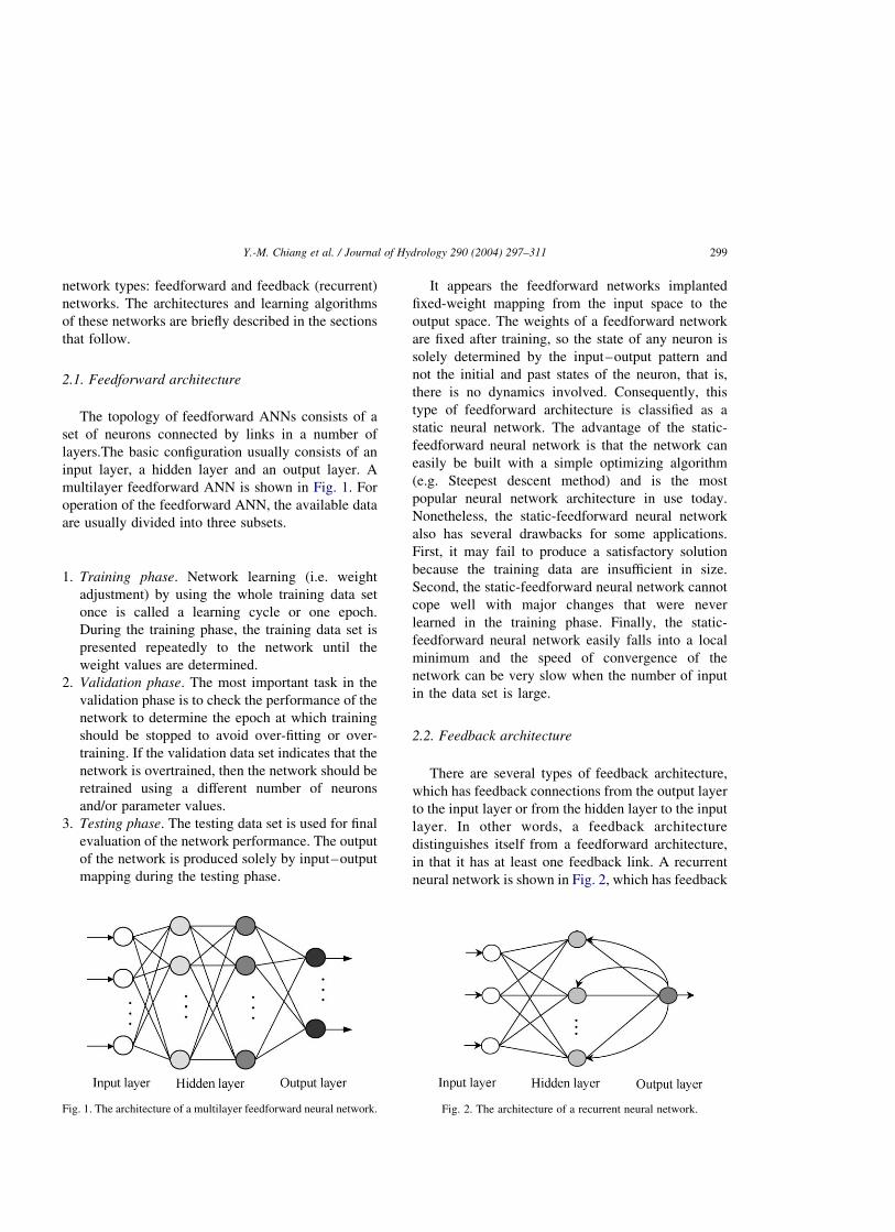
The topology of feedforward ANNs consists of a

set of neurons connected by links in a number of

layers.The basic configuration usually consists of an

input layer, a hidden layer and an output layer. A

multilayer feedforward ANN is shown in Fig. 1. For

operation of the feedforward ANN, the available data

are usually divided into three subsets.

1. Training phase. Network learning (i.e. weight

adjustment) by using the whole training data set

once is called a learning cycle or one epoch.

During the training phase, the training data set is

presented repeatedly to the network until the

weight values are determined.

2. Validation phase. The most important task in the

validation phase is to check the performance of the

network to determine the epoch at which training

should be stopped to avoid over-fitting or over-

training. If the validation data set indicates that the

network is overtrained, then the network should be

retrained using a different number of neurons

and/or parameter values.

3. Testing phase. The testing data set is used for final

evaluation of the network performance. The output

of the network is produced solely by input–output

mapping during the testing phase.

It appears the feedforward networks implanted

fixed-weight mapping from the input space to the

output space. The weights of a feedforward network

are fixed after training, so the state of any neuron is

solely determined by the input–output pattern and

not the initial and past states of the neuron, that is,

there is no dynamics involved. Consequently, this

type of feedforward architecture is classified as a

static neural network. The advantage of the static-

feedforward neural network is that the network can

easily be built with a simple optimizing algorithm

(e.g. Steepest descent method) and is the most

popular neural network architecture in use today.

Nonetheless, the static-feedforward neural network

also has several drawbacks for some applications.

First, it may fail to produce a satisfactory solution

because the training data are insufficient in size.

Second, the static-feedforward neural network cannot

cope well with major changes that were never

learned in the training phase. Finally, the static-

feedforward neural network easily falls into a local

minimum and the speed of convergence of the

network can be very slow when the number of input

in the data set is large.

2.2. Feedback architecture

There are several types of feedback architecture,

which has feedback connections from the output layer

to the input layer or from the hidden layer to the input

layer. In other words, a feedback architecture

distinguishes itself from a feedforward architecture,

in that it has at least one feedback link. A recurrent

neural network is shown in Fig. 2, which has feedback

Fig. 1. The architecture of a multilayer feedforward neural network. Fig. 2. The architecture of a recurrent neural network.

Y.-M. Chiang et al. / Journal of Hydrology 290 (2004) 297–311 299

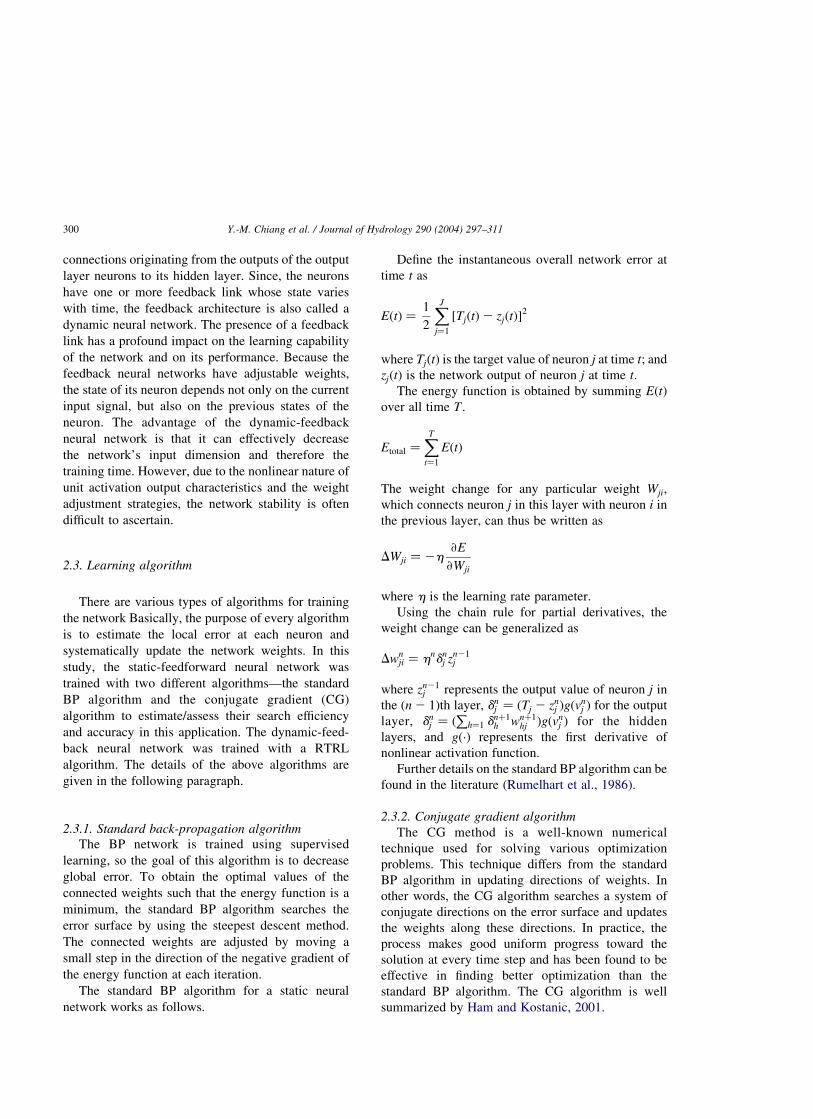
connections originating from the outputs of the output

layer neurons to its hidden layer. Since, the neurons

have one or more feedback link whose state varies

with time, the feedback architecture is also called a

dynamic neural network. The presence of a feedback

link has a profound impact on the learning capability

of the network and on its performance. Because the

feedback neural networks have adjustable weights,

the state of its neuron depends not only on the current

input signal, but also on the previous states of the

neuron. The advantage of the dynamic-feedback

neural network is that it can effectively decrease

the network’s input dimension and therefore the

training time. However, due to the nonlinear nature of

unit activation output characteristics and the weight

adjustment strategies, the network stability is often

difficult to ascertain.

2.3. Learning algorithm

There are various types of algorithms for training

the network Basically, the purpose of every algorithm

is to estimate the local error at each neuron and

systematically update the network weights. In this

study, the static-feedforward neural network was

trained with two different algorithms—the standard

BP algorithm and the conjugate gradient (CG)

algorithm to estimate/assess their search efficiency

and accuracy in this application. The dynamic-feed-

back neural network was trained with a RTRL

algorithm. The details of the above algorithms are

given in the following paragraph.

2.3.1. Standard back-propagation algorithmThe BP network is trained using supervised

learning, so the goal of this algorithm is to decrease

global error. To obtain the optimal values of the

connected weights such that the energy function is a

minimum, the standard BP algorithm searches the

error surface by using the steepest descent method.

The connected weights are adjusted by moving a

small step in the direction of the negative gradient of

the energy function at each iteration.

The standard BP algorithm for a static neural

network works as follows.

Define the instantaneous overall network error at

time t as

EðtÞ ¼1

2

XJ

j¼1

½TjðtÞ2 zjðtÞ�2

where TjðtÞ is the target value of neuron j at time t; and

zjðtÞ is the network output of neuron j at time t:

The energy function is obtained by summing EðtÞ

over all time T :

Etotal ¼XTt¼1

EðtÞ

The weight change for any particular weight Wji;

which connects neuron j in this layer with neuron i in

the previous layer, can thus be written as

DWji ¼ 2h›E

›Wji

where h is the learning rate parameter.

Using the chain rule for partial derivatives, the

weight change can be generalized as

Dwnji ¼ hndn

j zn21j

where zn21j represents the output value of neuron j in

the ðn 2 1Þth layer, dnj ¼ ðTj 2 zn

j Þgðvnj Þ for the output

layer, dnj ¼ ð

Ph¼1 d

nþ1h wnþ1

hj Þgðvnj Þ for the hidden

layers, and gð·Þ represents the first derivative of

nonlinear activation function.

Further details on the standard BP algorithm can be

found in the literature (Rumelhart et al., 1986).

2.3.2. Conjugate gradient algorithm

The CG method is a well-known numerical

technique used for solving various optimization

problems. This technique differs from the standard

BP algorithm in updating directions of weights. In

other words, the CG algorithm searches a system of

conjugate directions on the error surface and updates

the weights along these directions. In practice, the

process makes good uniform progress toward the

solution at every time step and has been found to be

effective in finding better optimization than the

standard BP algorithm. The CG algorithm is well

summarized by Ham and Kostanic, 2001.


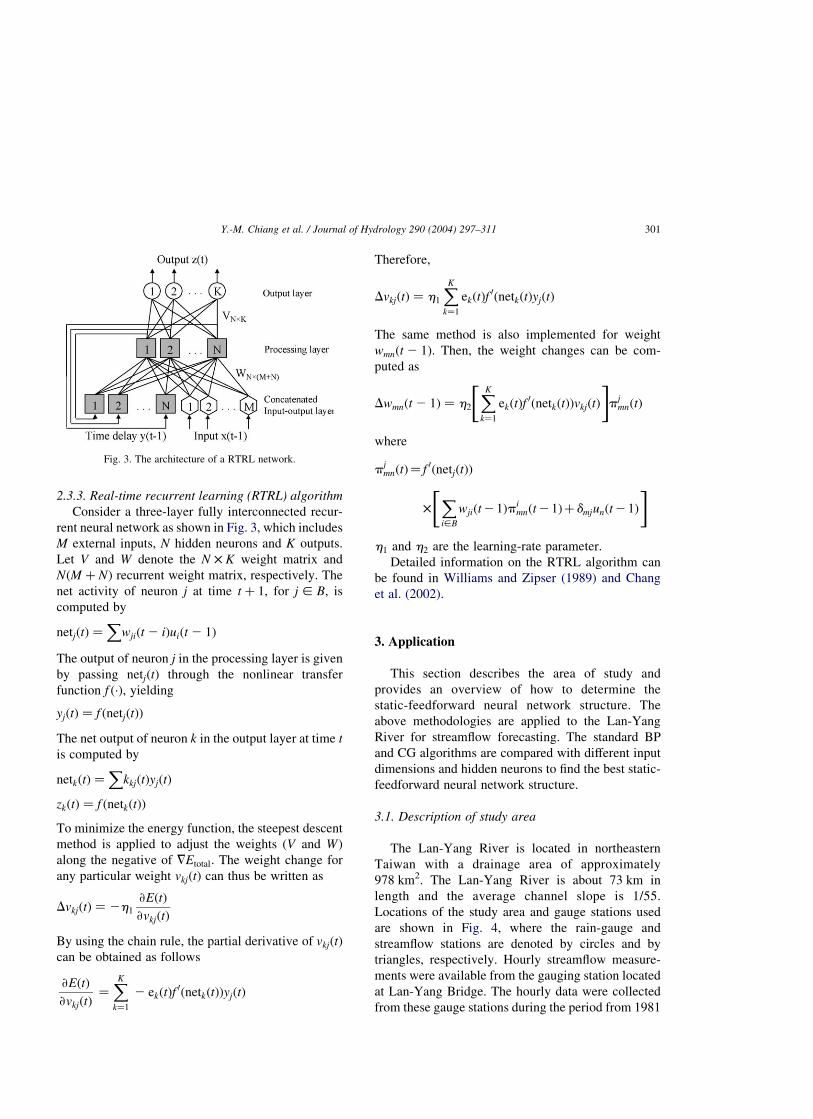
2.3.3. Real-time recurrent learning (RTRL) algorithm

Consider a three-layer fully interconnected recur-

rent neural network as shown in Fig. 3, which includes

M external inputs, N hidden neurons and K outputs.

Let V and W denote the N £ K weight matrix and

NðM þ NÞ recurrent weight matrix, respectively. The

net activity of neuron j at time t þ 1; for j [ B; is

computed by

netjðtÞ ¼X

wjiðt 2 iÞuiðt 2 1Þ

The output of neuron j in the processing layer is given

by passing netjðtÞ through the nonlinear transfer

function f ð·Þ; yielding

yjðtÞ ¼ f ðnetjðtÞÞ

The net output of neuron k in the output layer at time t

is computed by

netkðtÞ ¼X

kkjðtÞyjðtÞ

zkðtÞ ¼ f ðnetkðtÞÞ

To minimize the energy function, the steepest descent

method is applied to adjust the weights ðV and WÞ

along the negative of 7Etotal: The weight change for

any particular weight vkjðtÞ can thus be written as

DvkjðtÞ ¼ 2h1

›EðtÞ

›vkjðtÞ

By using the chain rule, the partial derivative of vkjðtÞ

can be obtained as follows

›EðtÞ

›vkjðtÞ¼

XKk¼1

2 ekðtÞf0ðnetkðtÞÞyjðtÞ

Therefore,

DvkjðtÞ ¼ h1

XKk¼1

ekðtÞf0ðnetkðtÞyjðtÞ

The same method is also implemented for weight

wmnðt 2 1Þ: Then, the weight changes can be com-

puted as

Dwmnðt 2 1Þ ¼ h2

XKk¼1

ekðtÞf0ðnetkðtÞÞvkjðtÞ

" #pj

mnðtÞ

where

pjmnðtÞ ¼ f 0ðnetjðtÞÞ

�Xi[B

wjiðt21Þpimnðt21Þþdmjunðt21Þ

" #

h1 and h2 are the learning-rate parameter.

Detailed information on the RTRL algorithm can

be found in Williams and Zipser (1989) and Chang

et al. (2002).

3. Application

This section describes the area of study and

provides an overview of how to determine the

static-feedforward neural network structure. The

above methodologies are applied to the Lan-Yang

River for streamflow forecasting. The standard BP

and CG algorithms are compared with different input

dimensions and hidden neurons to find the best static-

feedforward neural network structure.

3.1. Description of study area

The Lan-Yang River is located in northeastern

Taiwan with a drainage area of approximately

978 km2. The Lan-Yang River is about 73 km in

length and the average channel slope is 1/55.

Locations of the study area and gauge stations used

are shown in Fig. 4, where the rain-gauge and

streamflow stations are denoted by circles and by

triangles, respectively. Hourly streamflow measure-

ments were available from the gauging station located

at Lan-Yang Bridge. The hourly data were collected

from these gauge stations during the period from 1981

Fig. 3. The architecture of a RTRL network.


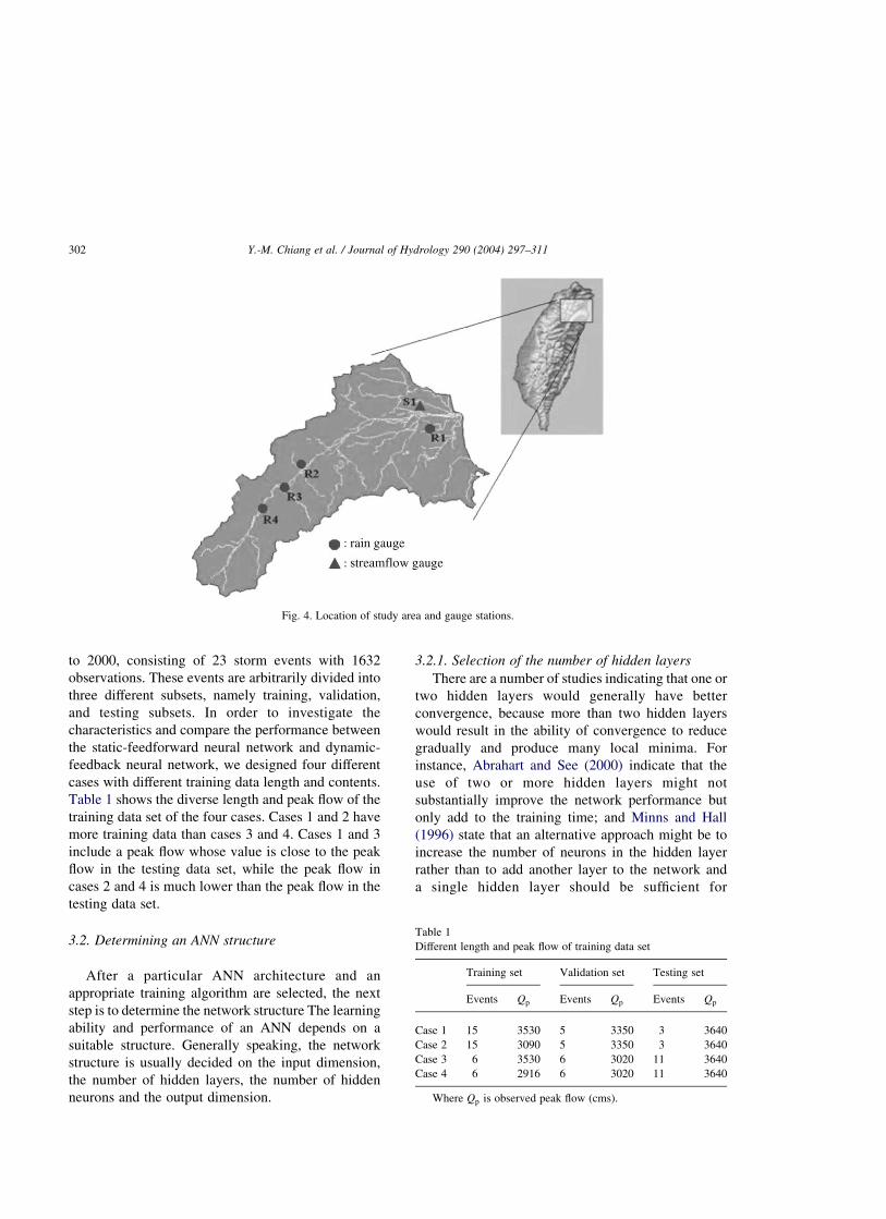
to 2000, consisting of 23 storm events with 1632

observations. These events are arbitrarily divided into

three different subsets, namely training, validation,

and testing subsets. In order to investigate the

characteristics and compare the performance between

the static-feedforward neural network and dynamic-

feedback neural network, we designed four different

cases with different training data length and contents.

Table 1 shows the diverse length and peak flow of the

training data set of the four cases. Cases 1 and 2 have

more training data than cases 3 and 4. Cases 1 and 3

include a peak flow whose value is close to the peak

flow in the testing data set, while the peak flow in

cases 2 and 4 is much lower than the peak flow in the

testing data set.

3.2. Determining an ANN structure

After a particular ANN architecture and an

appropriate training algorithm are selected, the next

step is to determine the network structure The learning

ability and performance of an ANN depends on a

suitable structure. Generally speaking, the network

structure is usually decided on the input dimension,

the number of hidden layers, the number of hidden

neurons and the output dimension.

3.2.1. Selection of the number of hidden layers

There are a number of studies indicating that one or

two hidden layers would generally have better

convergence, because more than two hidden layers

would result in the ability of convergence to reduce

gradually and produce many local minima. For

instance, Abrahart and See (2000) indicate that the

use of two or more hidden layers might not

substantially improve the network performance but

only add to the training time; and Minns and Hall

(1996) state that an alternative approach might be to

increase the number of neurons in the hidden layer

rather than to add another layer to the network and

a single hidden layer should be sufficient for

Fig. 4. Location of study area and gauge stations.

Table 1

Different length and peak flow of training data set

Training set Validation set Testing set

Events Qp Events Qp Events Qp

Case 1 15 3530 5 3350 3 3640

Case 2 15 3090 5 3350 3 3640

Case 3 6 3530 6 3020 11 3640

Case 4 6 2916 6 3020 11 3640

Where Qp is observed peak flow (cms).


the majority of real-world applications. Therefore, a

single hidden layer was adopted in this work.

3.2.2. Selection of input and output dimension

While static-feedforward neural networks are

very popular, they lack feedback connections to

effectively remember and handle the previous states

of information. One way that information can be

introduced in static-feedforward neural networks is

to input a time delay pattern that constitutes the

tapped delay line information. Therefore, this net-

work must determine the input variables, output

variables and the lag time of the basin before

constructing rainfall–runoff procedures in order to

increase its accuracy. In general, the selection of

input variables and output variables is problem

dependent. The appropriate input variables will

allow the network to successfully map to the desired

output and avoid loss of important information. In

the present study, the input dimensions are deter-

mined by the input variables and the lag time. To

determine an appropriate static-feedforward neural

network structure for forecasting the streamflow at

time t þ 1 in this selected basin, we develop four

different models for the standard BP and CG

algorithms, namely:

Model 1: Qðt þ 1Þ ¼ f ðQðtÞ; R1ðtÞ; R2ðtÞ; R3ðtÞ;

R4ðtÞÞ

Model 2: Qðt þ 1Þ ¼ f ðQðtÞ; Qðt 2 1Þ; R1ðtÞ;

R1ðt 2 1Þ; R2ðtÞ; R2ðt 2 1Þ; R3ðtÞ; R3ðt 2 1Þ;

R4ðtÞ; R4ðt 2 1ÞÞ

Model 3: Qðt þ 1Þ ¼ f ðQðtÞ; Qðt 2 1Þ; Qðt 2 2Þ;

R1ðtÞ; R1ðt 2 1Þ; R1ðt 2 2Þ; R2ðtÞ; R2ðt 2 1Þ;

R2ðt 2 2Þ; R3ðtÞ; R3ðt 2 1Þ; R3ðt 2 2Þ; R4ðtÞ;

R4ðt 2 1Þ; R4ðt 2 2ÞÞ

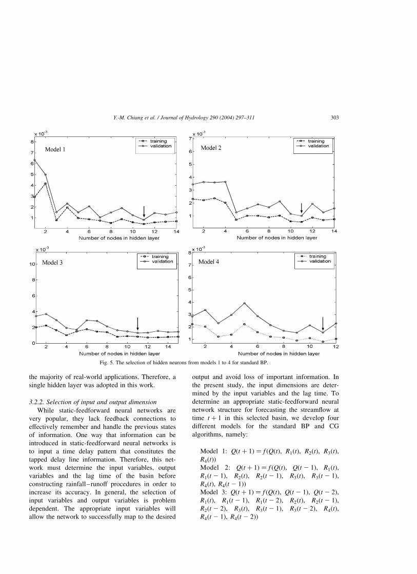
Fig. 5. The selection of hidden neurons from models 1 to 4 for standard BP.


Model 4: Qðt þ 1Þ ¼ f ðQðtÞ; Qðt 2 1Þ; Qðt 2 2Þ;

Qðt 2 3Þ; R1ðtÞ; R1ðt 2 1Þ; R1ðt 2 2Þ; R1ðt 2 3Þ;

R2ðtÞ; R2ðt 2 1Þ; R2ðt 2 2Þ; R2ðt 2 3Þ; R3ðtÞ;

R3ðt 2 1Þ; R3ðt 2 2Þ; R3ðt 2 3Þ; R4ðtÞ; R4ðt 2 1Þ;

R4ðt 2 2Þ; R4ðt 2 3ÞÞ

where Qðt 2 iÞ represents the value of the Lan-Yang

Bridge streamflow gauge station at time t 2 i; and

R1ðt 2 iÞ; R2ðt 2 iÞ; R3ðt 2 iÞ and R4ðt 2 iÞ rep-

resents the precipitation of the four rainfall gauge

stations at time t 2 i: Because the drainage area of

the study watershed is less than 1000 km2 and the

basin slope is quite steep, the time of concentration

is short. Consequently, the input pattern is focused

on the previous one to 3 h information only. Also,

because of the feedback quality of recurrent neural

networks, their input dimensions are values of each

gauge station at the present time t; this is a

particular characteristic as far as the dynamic-

feedback neural network is concerned.

3.2.3. Selection of the number of hidden neurons

The determination of the appropriate number of

hidden neurons is very important for the success of

the ANNs. If the hidden layer has too many

neurons this may cause each hidden neuron to

memorize one of the input patterns, and thereby

reduce the generalization capabilities and increase

the training time but without significant improve-

ment in training results (Ranjithan et al., 1993).

Imrie et al. (2000) indicate that too few hidden

neurons may have insufficient degrees of freedom

to capture the underlying relationships in the data.

Since, there is not a systematic or standard way to

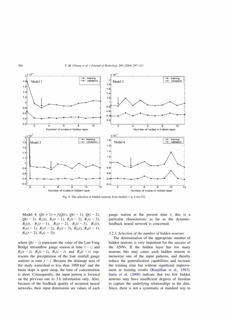
Fig. 6. The selection of hidden neurons from models 1 to 4 for CG.


decide on the number of neurons in the hidden

layer, the best way to select the hidden neurons is

by trial-and-error.

3.3. Selecting the best static-feedforward neural

network structure

First, we use case 1 with four different input

models to determine the standard BP and CG

network structures by using trial-and-error. Figs. 5

and 6 show the selection of the hidden neurons

from model 1 to model 4 for standard BP and CG,

respectively. The hidden neurons from 1 to 15 are

varied in each model and all the simulations are

terminated after 10,000 iterations. Tables 2 and 3

show the comparison of different models for

standard BP and CG, respectively, and the

performance of different models is presented

based on the criteria of mean absolute error

(MAE) and root mean square error (RMSE) as

shown below:

MAE ¼

XNt¼1

lðQsimðtÞ2 QobsðtÞÞl

N

RMSE ¼

ffiffiffiffiffiffiffiffiffiffiffiffiffiffiffiffiffiffiffiffiffiffiffiffiffiffiffiffiffiXNt¼1

ðQsimðtÞ2 QobsðtÞÞ2

N

vuuuutwhere Qsim is the forecasted value, Qobs is

the observed value, and N is the number of data

points.

The results show that Model 3 produces the best

performance for both the standard BP and CG

network structures. This result indirectly provides

evidence that the average lag time is no more than

3 h. Comparing the results in Table 2 and 3, it is

easy to tell that the CG method is superior to the

standard BP method in all the models and phases.

Consequently, we only use the CG algorithm for

training the static-feedforward neural network and

compare with RTRL.

4. Results and discussion

The input dimensions of RTRL are five which are

established by using the current four rain-gauges and

the streamflow data, while the processing layer is

constructed to have five neurons. To compare the

model accuracy of CG and RTRL, the performances

of these two methods are evaluated based on the

criteria of MAE, RMSE, relative mean absolute error

(RMAE) and Q̂p: The RMAE and Q̂p are defined as

follows

RMAE ¼MAE�Q

Table 2

Comparison of different standard BP architectures

Architecture MAE RMSE

Training Validation Training Validation

Model 1 5-11-1 85 93 195 209

Model 2 10-11-1 106 107 243 212

Model 3 15-11-1 89 90 197 171

Model 4 20-11-1 107 119 252 292

Table 3

Comparison of different CG architectures

Architecture MAE RMSE

Training Validation Training Validation

Model 1 5-3-1 49 52 110 115

Model 2 10-2-1 48 53 103 103

Model 3 15-5-1 45 48 97 105

Model 4 20-4-1 53 53 113 120

Table 4

Results of the CG and RTRL for case 1

Case 1 Qp Q̂p MAE RMAE RMSE

Training

CG 3530 2501 45 0.078 97

RTRL 2700 52 0.090 110

Validation

CG 3350 3294 48 0.093 105

RTRL 3220 59 0.114 149

Testing

CG 3640 2790 59 0.078 118

RTRL 3339 83 0.110 166


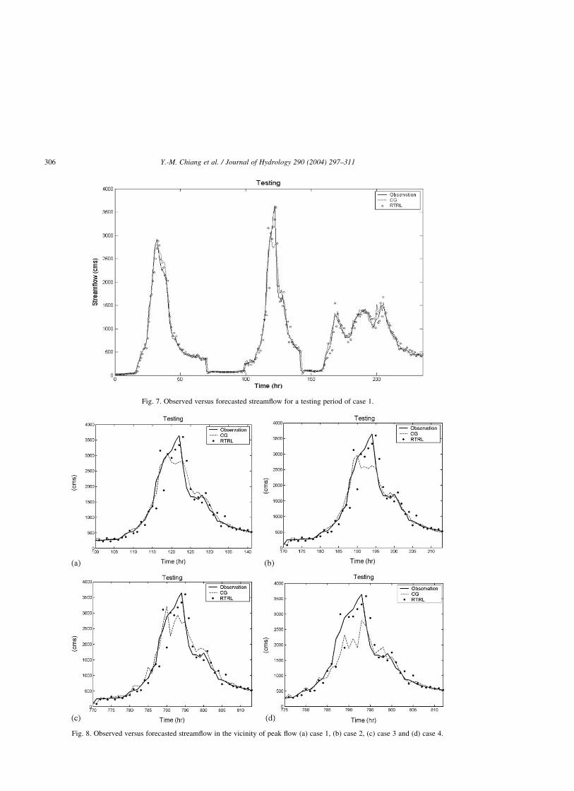
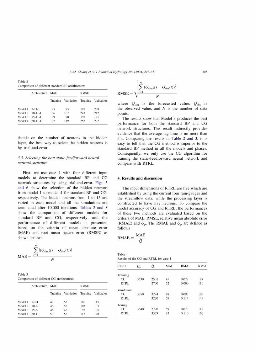
Fig. 7. Observed versus forecasted streamflow for a testing period of case 1.

Fig. 8. Observed versus forecasted streamflow in the vicinity of peak flow (a) case 1, (b) case 2, (c) case 3 and (d) case 4.


Q̂p is the estimated value at the time that the observed

peak flow occurred (cms).

Table 4 summarizes the comparative results of the

CG and RTRL methods for case 1. It appears that both

methods produce good forecasting of the streamflow

in all phases. We can also find that the CG method

obtains better performance (in terms of small MAE,

RMAE, and RMSE) than the RTRL, because of

sufficient training length and content in case 1.

However, the Q̂p values produced by the RTRL

method are superior to CG. Fig. 7 shows a comparison

of observed versus forecasted hourly streamflow for a

testing period of case 1. Fig. 8(a) is the enlarged peak

flow of case 1, so we can easily distinguish between

the two models’ performance.

The results of both methods for case 2–4 are

presented in Tables 5–7. Fig. 8(b–d) show the

observed versus forecasted streamflow by CG and

RTRL in the vicinity of peak flow in cases 2–4,

respectively. In the training stage, the CG method has

slightly better performance than the RTRL in all three

cases; however, the RTRL method produces much

better performance than the CG method in terms of

smaller MAE, RMAE, RMSE and high Q̂p value in

testing phases of all cases. The results demonstrate

that RTRL is relatively stable and performs well in all

cases, whereas CG presents satisfying performance in

the testing phase only when the training data has

enough length and sufficient contents.

Moreover, another important observation that can

be made from the static-feedforward neural network

forecasted result is with reference to the selection of

the training data set. Fig. 9 depicts the scatter plot of

CG of all cases. Fig. 9(a) shows the reasonable and

consistent performance in all three phases in case 1.

Fig. 9(b) shows the model performance for case 2

which includes the same training length of data sets

as case 1, but no extreme events are included. It

appears the accuracy in the testing phase was inferior

to case 1 even though a more accurate result is

obtained in the training phase. Fig. 9(d) represents a

good spread and the results in the training set of case

4 are the closest to the ideal line, which only has a

short length of data and is without extreme events.

However, in the testing phase, it has the widest

spread and departure from the ideal line results. That

is, it has the worst performance. Examining the

forecasted results of the CG method for cases 1–4, it

can be seen that the CG method produces much less

accurate results in the test phase than the training

phase for all the cases except case 1. These results

Table 5



Training

CG 3090 2986 43 0.075 79

RTRL 2892 49 0.086 96

Validation

CG 3350 3300 51 0.099 104

RTRL 3181 58 0.112 129

Testing

CG 3640 2633 111 0.135 225

RTRL 3329 102 0.124 225

Table 6



Training

CG 3530 2474 55 0.098 128

RTRL 2735 57 0.102 129

Validation

CG 3020 2861 47 0.093 88

RTRL 2741 37 0.074 79

Testing

CG 3640 2667 81 0.126 165

RTRL 3337 68 0.105 143

Table 7



Training

CG 2916 2725 40 0.082 70

RTRL 2818 47 0.097 84

Validation

CG 3020 2739 54 0.107 112

RTRL 2755 37 0.074 78

Testing

CG 3640 2790 113 0.168 249

RTRL 3315 74 0.110 158


might indicate that the static-feedforward neural

network with the CG algorithm could not produce

satisfactory results when there is not a sufficient and

adequate training data set to build a suitable input–

output relationship.

Fig. 10 depicts the scatter plot of RTRL for

all cases. Because of the continually updating

and learning characteristic of the RTRL network,

the operation is regarded as a whole procedure for

each case, different from the CG network that divides

available data into three phases. Fig. 10(a–d) shows

that the performance of RTRL of all four cases is quite

stable and consistent. It appears that the RTRL

produces acceptable results insensitive to the length

and contents of the data set. Moreover, the RTRL has

the ability to capture the main trend or characteristics

Fig. 9. Comparison of observed and forecasted streamflow of CG (a) case 1, (b) case 2, (c) case 3 and (d) case 4.


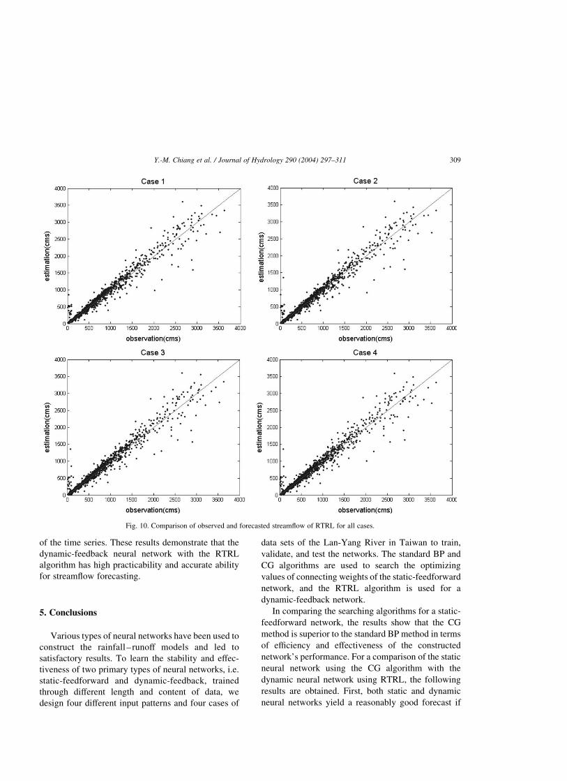
of the time series. These results demonstrate that the

dynamic-feedback neural network with the RTRL

algorithm has high practicability and accurate ability

for streamflow forecasting.

5. Conclusions

Various types of neural networks have been used to

construct the rainfall–runoff models and led to

satisfactory results. To learn the stability and effec-

tiveness of two primary types of neural networks, i.e.

static-feedforward and dynamic-feedback, trained

through different length and content of data, we

design four different input patterns and four cases of

data sets of the Lan-Yang River in Taiwan to train,

validate, and test the networks. The standard BP and

CG algorithms are used to search the optimizing

values of connecting weights of the static-feedforward

network, and the RTRL algorithm is used for a

dynamic-feedback network.

In comparing the searching algorithms for a static-

feedforward network, the results show that the CG

method is superior to the standard BP method in terms

of efficiency and effectiveness of the constructed

network’s performance. For a comparison of the static

neural network using the CG algorithm with the

dynamic neural network using RTRL, the following

results are obtained. First, both static and dynamic

neural networks yield a reasonably good forecast if

Fig. 10. Comparison of observed and forecasted streamflow of RTRL for all cases.


there is adequate length and content of data included

(case 1). Even though, the static-feedforward network

produces slightly better performance (in terms of

small MAE and RMSE values) than the dynamic

network, we notice that the dynamic network better

captures the peak flows. Second, in cases 2–4, for

which non-sufficient length or content of data is

involved in the training phase, the results show that

the dynamic network has significantly better perform-

ance than the static network, especially in the testing

phase. The static network produces poor performance

(in terms of larger MAE and RMSE, and highly

underestimates the peak flow) in the testing phase.

These results suggest that the static-feedforward

neural network with the CG algorithm could produce

satisfactory results only when there is a sufficient and

adequate training data set. Third, the feedforward

neural networks executed fixed-weight mapping from

the input space to the output space. Due to fixed

weights, the output is solely determined by the present

input state to the network and not the initial and past

states of the neurons in the network. Consequently,

the input–output mapping of the feedforward neural

networks is static and the networks would be trained

to store the information content in the training data

and could only produce the memory structures within

processes. On the contrary, the feedback neural

networks do allow initial and past state involvement

along with serial processing. These networks provide

a representation of dynamic internal feedback loops to

store information for later use, to enhance the

efficiency of learning, and to carry out the sequential

temporal behavior. Furthermore, the RTRL algorithm

helps to continually update the feedback neural

network for learning, and this feature is especially

important and useful for grasping the extraordinary

time-varying characteristics of rainfall – runoff

processes.

Acknowledgements

This paper is based on partial work supported by

National Science Council, ROC (Grant No. NSC91-

2313-B-002-343). In addition, the authors are

indebted to the reviewers for their valuable comments

and suggestions.

References

Abrahart, R.J., See, L., 2000. Comparing neural network and

autoregressive moving average techniques for the provision of

continuous river flow forecasts in two contrasting catchments.

Hydrological Processes 14, 2157–2172.

ASCE Task Committee on Application of Artificial Neural

Networks in Hydrology, 2000a. Artificial neural networks in

hydrology I: preliminary concepts. Journal of Hydrologic

Engineering 5 (2), 115–123.

ASCE Task Committee on Application of Artificial Neural

Networks in Hydrology, 2000b. Artificial neural networks in

hydrology II: Hydrologic applications. Journal of Hydrologic

Engineering 5 (2), 124–137.

Beven, K., 2001. How far can we go in distributed hydrological

modeling. Hydrology and Earth System Science 5, 1–12.

Cameron, D., Kneale, P., See, L., 2002. An evaluation of traditional

and a neural net modeling approach to flood forecasting for an

upland catchment. Hydrological Processes 16, 1033–1046.

Campolo, M., Andreussi, P., Soldati, A., 1999. River flood

forecasting with a neural network model. Water Resources

Research 35 (4), 1191–1197.

Chang, L.C., Chang, F.J., 2001. Intelligent control for modeling of

real time reservoir operation. Hydrological Processes 15,

1621–1634.

Chang, F.J., Chen, Y.C., 2001. A counterpropagation fuzzy-neural

network modeling approach to real time stream flow prediction.

Journal of Hydrology 245, 153–164.

Chang, F.J., Chen, Y.C., 2003. Estuary water-stage forecasting by

using Radial Basis Function neural network. Journal of

Hydrology 270, 158–166.

Chang, F.J., Liang, J.M., Chen, Y.C., 2001. Flood forecasting using

radial basis function neural network. IEEE Transactions on

Systems, Man and Cybernetics Part C: Applications and

Reviews 31 (4), 530–535.

Chang, F.J., Chang, L.C., Huang, H.L., 2002. Real-time recurrent

neural network for stream-flow forecasting. Hydrological

Processes 16, 2577–2588.

Chang, L.C., Chang, F.J., Chiang, Y.M., 2004. A two-step ahead

recurrent neural network for streamflow forecasting. Hydro-

logical Processes 18, 81–92.

Coulibaly, P., Anctil, F., Bobee, B., 2001. Multivariate reservoir

inflow forecasting using temporal neural networks. Journal of

Hydrologic Engineering 6 (5), 367–376.

Dawson, C.W., Wilby, R.L., 1998. An artificial neural network

approach to rainfall–runoff modeling. Hydrological Sciences 43

(1), 47–67.

Dawson, C.W., Wilby, R.L., 2001. Hydrological modeling using

artificial neural networks. Progress in Physical Geography 25

(1), 80–108.

Elshorbagy, A., Simonovic, S.P., Panu, U.S., 2000. Performance

evaluation of artificial neural networks for runoff prediction.

Journal of Hydrologic Engineering ASCE 5 (4), 424–427.

French, M.N., Krajewski, W.F., Cuykendall, R.R., 1992. Rainfall

forecasting in space and time using a neural network. Journal of

Hydrology 137, 1–31.


Golob, R., Stokelj, T., Grgic, D., 1998. Neural-network-based water

inflow forecasting. Control Engineering Practice 6, 593–600.

Govindaraju, R.S., Ruo, A.R., 2000. Artificial Neural Networks in

Hydrology. Kluwer Academic Publishers, Dordrecht.

Ham, F.M., Kostanic, I., 2001. Principles of neurocomputing for

science and engineering. McGraw-Hill, New York.

Haykin, S., 1999. Neural Network: a Comprehensive Foundation,

second ed., Prentice Hall, Englewood, Cliffs, NJ.

Hopfield, J.J., 1982. Neural networks and physical systems with

emergent collective computational abilities. Proceedings of the

National Academy of Sciences of the United States of America

79 (8), 2254–2258.

Hsu, K.L., Gupta, H.V., Sorooshian, S., 1995. Artificial neural

network modeling of the rainfall– runoff process. Water

Resources Research 31 (10), 2517–2530.

Hydrological Engineering Center, 1990. HEC-1 Flood Hydrograph

Package, Program Users Manual. US Army Crops of Engineers:

Davis, C.A.,.

Imrie, C.E., Durucan, S., Korre, A., 2000. River flow prediction

using artificial neural network: generalisation beyond the

calibration range. Journal of Hydrology 233, 138–153.

Karunanithi, N., Grenney, W.J., Whitley, D., 1994. Neural network

for river flow prediction. Journal of Computing in Civil

Engineering 8, 201–220.

Kohonen, T., 1982. Self-organized formation of topologically

correct feature maps. Biological Cybernetics 43, 59–69.

Luk, K.C., Ball, J.E., Sharma, A., 2000. A study of optimal model

lag and spatial inputs to artificial neural network for rainfall

forecasting. Journal of Hydrology 227, 56–65.

Maier, H.R., Dandy, G.C., 2000. Neural networks for the prediction

and forecasting of water resources variables: a review of

modelling issues and applications. Environmental Modelling

and Software 15 (1), 101–124.

McCulloch, W.S., Pitts, W., 1943. A logical calculus of the ideas

immanent in nervous activity. Bulletin of Mathematical

Biophysics 5, 115–133.

Minns, A.W., Hall, M.J., 1996. Artificial neural networks as

rainfall–runoff models. Hydrological Sciences 41 (3), 399–417.

Powell, M.J.D., 1985. Radial basis functions for multivariable

interpolation: a review, IMA Conference on Algorithms for the

Approximation of Functions and Data, RMCS, Shrivenham,

England, pp. 143–167.

Ranjithan, S., Eheart, J.W., Garrett, J.H. Jr., 1993. Neural network-

based screening for groundwater reclamation under uncern-

tainty. Water Resources Research 29 (3), 563–574.

Rumelhart, D.E., Hinton, G.E., Williams, R.J., 1986. Learning

internal representations by error propagation. Parallel Distrib-

uted Processing 1, 318–362.

Sajikumar, N., Thandaveswara, B.S., 1999. A non-linear rainfall–

runoff model using an artificial neural network. Journal of

Hydrology 216, 32–55.

Salas, J.D., Tabios, G.Q., Bartolini, P., 1985. Approaches to

multivariate modeling of water resources time series. Water

Resources Bulletin 21 (4), 683–708.

Shamseldin, A.Y., 1997. Application of a neural network technique

to rainfall– runoff modeling. Journal of Hydrology 199,

272–294.

Sivakumar, B., Jayawardena, A.W., Fernando, T.M.K.G., 2002.

River flow forecasting-use of phase-space reconstruction and

artificial neural networks approaches. Journal of Hydrology 265,

225–245.

Smith, J., Eli, R.N., 1995. Neural network models of rainfall–runoff

process. Journal of Water Resources Planning and Management

121 (6), 499–508.

Thirumalaiah, K., Deo, M.C., 1998. River stage forecasting using

artificial neural network. Journal of Hydrologic Engineering

3 (1), 26–32.

Tokar, A.S., Johnson, P.A., 1999. Rainfall–runoff modeling using

artificial neural networks. Journal of Hydrologic Engineering 4

(3), 232–239.

Williams, R., Zipser, D., 1989. A learning algorithm for continually

running fully recurrent neural network. Neural Computation 1,

270–280.

Zealand, C.M., Burn, D.H., Simonovic, S.P., 1999. Short term

stream flow forecasting using artificial neural networks. Journal

of Hydrology 214, 32–48.


Comparison of static-feedforward and dynamic-feedback neural

Documents

Transcript of Comparison of static-feedforward and dynamic-feedback neural