Scholars' Mine Scholars' Mine

Masters Theses Student Theses and Dissertations

Spring 2013

Comparison of square root of time approach and statistical Comparison of square root of time approach and statistical

approach to minimize subjectivity in the determination of approach to minimize subjectivity in the determination of

minimum in-situ stress minimum in-situ stress

Soumitra Bhaskar Nande

Follow this and additional works at: https://scholarsmine.mst.edu/masters_theses

Part of the Petroleum Engineering Commons

Department: Department:

Recommended Citation Recommended Citation Nande, Soumitra Bhaskar, "Comparison of square root of time approach and statistical approach to minimize subjectivity in the determination of minimum in-situ stress" (2013). Masters Theses. 7100. https://scholarsmine.mst.edu/masters_theses/7100

This thesis is brought to you by Scholars' Mine, a service of the Missouri S&T Library and Learning Resources. This work is protected by U. S. Copyright Law. Unauthorized use including reproduction for redistribution requires the permission of the copyright holder. For more information, please contact scholarsmine@mst.edu.

COMPARISON OF SQUARE ROOT OF TIME APPROACH AND STATISTICAL

APPROACH TO MINIMIZE SUBJECTIVITY IN THE DETERMINATION OF

MINIMUM IN-SITU STRESS

By

SOUMITRA BHASKAR NANDE

A THESIS

Presented to the Faculty of the Graduate School of the

MISSOURI UNIVERSITY OF SCIENCE AND TECHNOLOGY

In Partial Fulfillment of the Requirements for the Degree

MASTER OF SCIENCE IN PETROLEUM ENGINEERING

2013

Approved by

Dr. Shari Dunn-Norman, Advisor

Dr. V. Samaranayake

Larry K. Britt

Dr. Ralph Flori

2013

Soumitra B.Nande

All Rights Reserved

iii

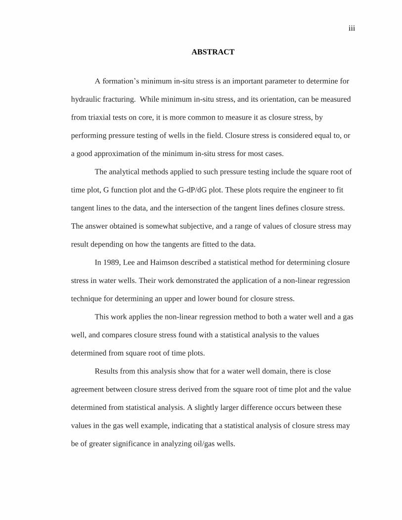
ABSTRACT

A formation‟s minimum in-situ stress is an important parameter to determine for

hydraulic fracturing. While minimum in-situ stress, and its orientation, can be measured

from triaxial tests on core, it is more common to measure it as closure stress, by

performing pressure testing of wells in the field. Closure stress is considered equal to, or

a good approximation of the minimum in-situ stress for most cases.

The analytical methods applied to such pressure testing include the square root of

time plot, G function plot and the G-dP/dG plot. These plots require the engineer to fit

tangent lines to the data, and the intersection of the tangent lines defines closure stress.

The answer obtained is somewhat subjective, and a range of values of closure stress may

result depending on how the tangents are fitted to the data.

In 1989, Lee and Haimson described a statistical method for determining closure

stress in water wells. Their work demonstrated the application of a non-linear regression

technique for determining an upper and lower bound for closure stress.

This work applies the non-linear regression method to both a water well and a gas

well, and compares closure stress found with a statistical analysis to the values

determined from square root of time plots.

Results from this analysis show that for a water well domain, there is close

agreement between closure stress derived from the square root of time plot and the value

determined from statistical analysis. A slightly larger difference occurs between these

values in the gas well example, indicating that a statistical analysis of closure stress may

be of greater significance in analyzing oil/gas wells.

iv

ACKNOWLEDGMENTS

This thesis would not have been possible without the guidance and the help of

several individuals who in one way or another contributed and extended their valuable

assistance in the preparation and completion of this study.

I would like to express my deep and sincere gratitude to my advisor, Dr. Shari

Dunn-Norman. Her wide knowledge and her logical way of thinking have been of great

value for me. Her understanding, encouraging and personal guidance have provided a

good basis for the present thesis.

I am deeply grateful to Dr. Samaranayake who introduced me to SAS and who

helped me with writing a program in SAS and performing statistical analysis on a data.

This work would not have been possible without his support.

I wish to express my warm and sincere thanks to Professor Larry K. Britt, for

providing the data, for a valuable advice and for friendly help. I also wish to thank City

Utilities for providing the data and for making this work possible.

My sincere thanks to my committee members, Dr. Ralph Flori, Dr. Samaranayake

and Professor Britt, for their constant support.

I owe my loving thanks to my family Aai, Baba and Dada, and my love Amruta.

Without their love, support and encouragement, this work was never possible. Thanks are

also due to my friends in Rolla and back in India. Thank You for always being there with

me.

Last but not the least, to the one above all of us, the omnipresent God, for

answering my prayers for giving me the strength to plod on despite my constitution

wanting to give up and throw in the towel, thank you so much Dear Lord.

v

TABLE OF CONTENTS

Page

ABSTRACT ....................................................................................................................... iii

ACKNOWLEDGMENTS..................................................................................................iv

LIST OF ILLUSTRATIONS ............................................................................................ vii

LIST OF TABLES ............................................................................................................. ix

NOMENCLATURE ........................................................................................................... x

SECTION

1. INTRODUCTION ................................................................................................ 1

2. LITERATURE REVIEW ..................................................................................... 4

3. SUBSURFACE STRESSES ................................................................................ 7

3.1.MOHR-COULOMB FAILURE ENVELOPE ........................................... 12

3.2. IN-SITU STRESS DETERMINATION ................................................... 14

3.3.IMPORTANCE OF MINIMUM IN-SITU STRESS IN TREATMENT

DESIGN.................................................................................................... 15

3.4. HYDRAULIC FRACTURING TREATMENT PRESSURE

PROFILE.……..........................................................................................17

4. HYDRAULIC FRACTURING PRESSURE TESTS AND THEIR

ANALYSES.......................................................................................................21

4.1.HYDRAULIC FRACTURING PRESSURE TESTS ................................ 21

4.2. FRACTURING PRESSURE ANALYSIS USING ANALYTICAL

TECHNIQUES………………………………………………………......29

4.3. SUBJECTIVITY ISSUES WITH ANALYTICAL METHODS.………..33

5. SQAURE ROOT OF TIME ANALYSIS FOR WATER WELL AND GAS

WELL.................................................................................................................37

vi

5.1. CU EXPLORATORY WELL # 1 (WATER WELL).…….......................37

5.2. CANADIAN GAS WELL # 2 .……...........................................................41

6. STATISTICAL APPROACH FOR CLOSURE STRESS CALCULATION.....45

6.1. NON LINEAR REGRESSION ANALYSIS.……....................................45

6.2. SAS.……....................................................................................................48

6.3. SAS PROGRAMMING……………………………………….................49

6.3.1. SAS Programming Statements...………………...…………….…..51

6.3.2. SAS Log File and Results File..……………………...……………52

7. STATISTICAL ANALYSIS OF THE DATA.......…..……………….………..55

7.1. THE 'NLIN' PROCEDURE....…....……………………….....……..........55

7.2. CU EXPLORATORY WELL # 1 (WATER WELL).…….......................57

7.3. CANADIAN GAS WELL # 2.……...........................................................62

8. RESULTS AND DISCUSSION.……................................................................66

9. CONCLUSION.……..........................................................................................68

APPENDICES

A. STIMPLAN ANALYSIS, DIGITALLY RECORDED CURVES AND

MODELED CURVES ....................................................................................... 70

B. OUTPUT TABLES FROM SAS.……..............................................................89

REFERENCES ............................................................................................................... 111

VITA .. ........................................................................................................................... 114

vii

LIST OF ILLUSTRATIONS

Figure Page

3.1. Force F acting on a plane at point P having an area A............................................8

3.2. Normal and Shear stresses acting in 2-D……………………………………………..9

3.3. General stress state in 3-D…………………………………………………………..11

3.4. Mohr's failure envelope..............................................................................................13

3.5. Stress gradients varying over depths………………………………………………..16

3.6. Surface pressure plot for fracturing treatment............................................................17

4.1. Idealized pump in/flowback test.……………………………………………….......22

4.2. Pump in/flowback test showing effects of different rates ………………………….22

4.3. Pump in/flowback test ……………………………………………………………...23

4.4. A typical pump in/decline test ………………………………………………….......25

4.5. Change of slope representing closure stress value for pump in/decline test….…….25

4.6. Rate v/s time plot for a typical step rate………...………...………………………...26

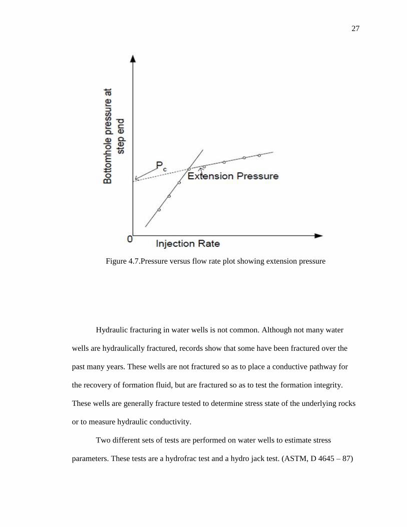
4.7. Pressure versus flow rate plot showing extension pressure…………………………27

4.8. A hydrofrac and hydrojack test..…………………………………………………….28

4.9. An example of square root of time plot analysis..…………………………………..31

4.10. An example of G-function plot analysis.…………………………………………..31

4.11. An example of G-dP/dG plot analysis..…………………………………………....32

4.12. Square root of time plot analysis showing Pc of 3428 psi.………………………..33

4.13. Square root of time plot analysis showing Pc of 2847 psi.………………………..34

4.14. Square root of time plot analysis showing Pc of 3003 psi.………………………..35

5.1. Hydrofrac test performed on test interval 9.………………………………………..38

viii

5.2. Hydrojack test performed on test interval 9.………………………………………..39

5.3. Square root time plot analysis for test interval 9.……………….…………………..40

5.4. Data plot for stress test in Canadian gas well # 2.…………………………………..42

5.5. Square root time analysis for stress test in Canadian gas well # 2.…………..……..43

5.6. Data plot for minifrac test in Canadian gas well # 2.…………………………….….44

5.7. Square root time analysis for minifrac test in Canadian gas well #2 .…………....…44

6.1. Curve fitting process and RMS graph using NLRA..………………………….……48

6.2. SAS enterprise guide showing program window..………………………………….50

6.3. A simple SAS program showing use of different statements.....…………………....52

6.4. SAS log file for the sample program..………………………………………………53

6.5. SAS output file showing results from a PROC statement.………………………….54

6.6. SAS results file..…………………………………………………………………….54

7.1. SAS program used for the study showing „nlin‟ procedure.………………………..56

7.2. Graph showing stabilized value of RMS for interval 9…………………………......60

7.3. Modeled curve (blue) extrapolated to Y axis for interval 9 …………………….…..61

7.4. RMS graph for stress test on Canadian gas well # 2 ………………………….…….63

7.5. Modeled curve (blue) extrapolated to Y axis for stress test …………………….…..64

7.6. Modeled curve extrapolated to Y axis for minifrac test ……………………………65

ix

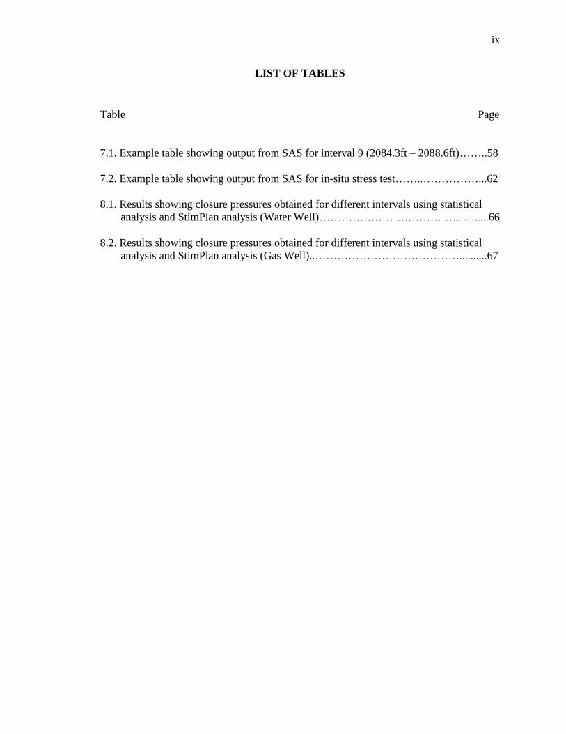
LIST OF TABLES

Table Page

7.1. Example table showing output from SAS for interval 9 (2084.3ft – 2088.6ft)……..58

7.2. Example table showing output from SAS for in-situ stress test……..……………...62

8.1. Results showing closure pressures obtained for different intervals using statistical

analysis and StimPlan analysis (Water Well)…………………………………….....66

8.2. Results showing closure pressures obtained for different intervals using statistical

analysis and StimPlan analysis (Gas Well)..…………………………………..........67

x

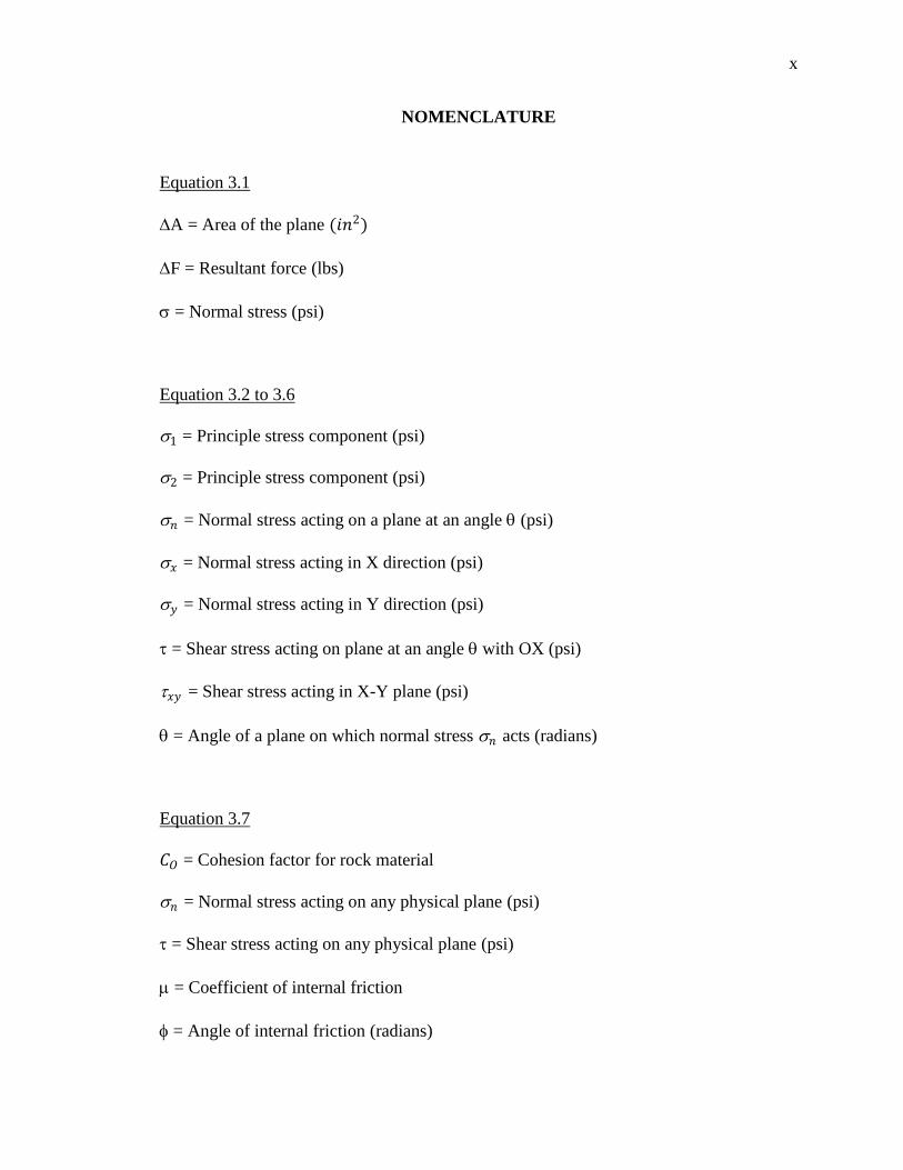
NOMENCLATURE

Equation 3.1

A = Area of the plane (𝑖𝑛2)

F = Resultant force (lbs)

= Normal stress (psi)

Equation 3.2 to 3.6

1 = Principle stress component (psi)

2 = Principle stress component (psi)

𝑛 = Normal stress acting on a plane at an angle (psi)

𝑥 = Normal stress acting in X direction (psi)

𝑦 = Normal stress acting in Y direction (psi)

= Shear stress acting on plane at an angle with OX (psi)

𝑥𝑦 = Shear stress acting in X-Y plane (psi)

= Angle of a plane on which normal stress 𝑛 acts (radians)

Equation 3.7

𝐶𝑂 = Cohesion factor for rock material

𝑛 = Normal stress acting on any physical plane (psi)

= Shear stress acting on any physical plane (psi)

= Coefficient of internal friction

= Angle of internal friction (radians)

xi

Equation 3.8

g = Acceleration due to gravity (ft/𝑠𝑒𝑐2)

h = Depth of the reservoir (ft)

𝑣 = Vertical stress acting on rock plane (psi)

= Density of the reservoir rock (pcf)

Equation 3.9

P = Pore pressure (psi)

= Poroelastic constant

2 = Intermediate principle stress (psi)

3 = Minimum principle stress (psi)

𝑣 = Vertical stress (psi)

= Poisson's ratio

Equation 6.1

𝑑1 = Pressure decay parameter

𝑑2 = Pressure decay parameter

𝑃𝑎𝑙 = Asymptotic pressure/ Reservoir pressure (psi)

𝑃𝑝𝑖 = Modeled pressure (psi)

t = Time since pumps have been shut down (minutes)

𝑡𝐿 = Time since fractures have been closed (minutes)

xii

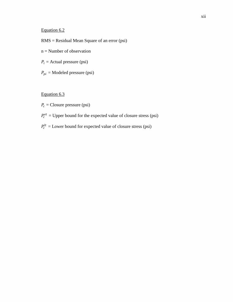
Equation 6.2

RMS = Residual Mean Square of an error (psi)

n = Number of observation

𝑃𝑖 = Actual pressure (psi)

𝑃𝑝𝑖 = Modeled pressure (psi)

Equation 6.3

𝑃𝑐 = Closure pressure (psi)

𝑃𝑐𝑒𝑡 = Upper bound for the expected value of closure stress (psi)

𝑃𝑐𝑙𝑡 = Lower bound for expected value of closure stress (psi)

1. INTRODUCTION

Since its introduction in 1947, hydraulic fracturing has had a significant impact on

well productivity and has become the primary means of increasing production. Over one

million oil and gas wells have been stimulated in the United States to date. Hydraulic

fracturing, combined with horizontal drilling, is the key technology enabling

development of unconventional reservoirs.

Hydraulic fracturing consists of initiating a fracture in the formation by pumping

fracturing fluid above the breakdown pressure of the formation, then propagating the

fracture by injecting fracturing fluid and proppant. When the treatment ends, pump

pressure is released, and the fluid in the fracture leaks off to the formation. The

formation gradually closes on the proppant, which acts to keep the fracture open. The

created fracture serves as a conductive pathway for the formation fluids to enter the well

bore.

Minimum in-situ stress is an important parameter as far as hydraulic fracturing is

considered. Minimum in-situ stress affects the pressures at which subsurface fractures

occur, and the orientation of the minimum in-situ stress affects fracture morphology.

Stress contrasts between adjacent formations control fracture height growth. Hence,

accurate determination of the minimum stress is very important in hydraulic fracturing

design.

If rock core samples are available, triaxial core testing may be conducted to

measure the magnitude and orientation of the principal stress. Either an analastic strain

2

recovery (ASR) technique or a differential strain curve method can be used. Both of these

are destructive testing methods and can only be used where core is available.

Minimum in-situ stress can also be determined from field methods, in particular

pressure testing. Pump in-fall off pressure testing is easier to apply and less expensive

than core analysis. Commonly applied pressure testing methods include step-rate tests

with shut in, micro frac or mini frac testing. Frequently, two or more of these tests may

be combined to verify the values obtained by pressure testing.

Closure stress, defined as the minimum fluid pressure inside the fracture required

to hold the fracture open, is equal to the minimum in-situ stress in most cases. Closure

stress is identified from the fall-off period following a pump-in, and is sometimes visible

as a point where the pressure fall off data changes slope. In most cases the closure stress

is not obvious from visual inspection of the recorded pressure fall-off data, and must be

determined with analytical methods.

Pressure transient methods are used to analyze the pressure versus time data

obtained from the pump in-fall off tests. These are square root of time plot, G-function

plot, G-dP/dG plot. In these methods a tangent is drawn to fall off period every time there

is a change in trend of decline. Change of slope indicates change in linear flow behavior

and taken to indicate that fracture is closing.

The difficulty with the analytical methods is that the closure pressure identified

may not be unique. It is possible to have the intersection of tangents over a range of

values. In some cases, there may be a hundred psi or more difference in the answers

obtained from different individual‟s analyses.

3

Regression analysis can be used to narrow down the range of uncertainty, and

identify the highest and lowest best values of the closure stress. A Non Linear Regression

Analysis (NLRA) has been identified and applied in this work. This method uses an

exponential pressure decay model to isolate the open fracture segment and provide a

small range over which a closure stress can be obtained.

This study presents a comparison of conventional analytical methods for

determining the closure stress with the NLRA. This study utilizes pressure testing data

from a water well and a gas well for comparison, demonstrating when regression is most

useful. City Utility project exploratory well # 1 is a water well at CU power plant located

in southwestern Missouri drilled for possible 𝐶𝑂2 sequestration. Lammote and Reagan

sandstones are pressure tested, for closure pressure, using water as the principal fluid.

The Canadian gas well # 2 is a new producing well in an existing major gas field and the

aim is to place optimum fracture stimulation treatment. The data contains an in-situ stress

test and a minifrac test which will be analyzed for closure pressure.

The regression method provided in this thesis may also be applied to other key

parameters of pressure analysis for hydraulic fracturing, such as fracture extension

pressure, instantaneous shut in pressure, and breakdown pressure. This thesis focuses on

closure stress because this is a key design parameter in hydraulic fracturing.

4

2. LITERATURE REVIEW

Many researchers have proposed methods to determine closure stress using

pressure fall off analysis. Many authors have suggested a variety of methods for the

determination of closure stress using different techniques.

Sigfried and Simmons (1978), Simmons and Richter (1976), Ren and Roegiers

(1983) conducted Differential Strain Curve Analysis (DSCA) on a core sample to

determine the magnitude of in-situ stresses. Van dam et al (2000) also conducted

laboratory experiments to determine the magnitude and direction of in-situ stresses. A.S.

Abou-Sayed presented a special laboratory technique to determine minimum in-situ stress

and in-situ stress contrast in absence of direct, field measured in-situ stress data. Holt et

al (2001) applied a discrete particle model to simulate coring and core reloading of a

cemented granular material formed under 3D state of stress.

Warpinski and Smith (1989) presented a good review of rock mechanics and

fracture geometry in which they state that in-situ stresses are clearly single most

important parameter controlling hydraulic fracturing. Different authors such as DeBree et

al (1978), Nolte K.G. (1988), Daneshy et al (1986), Warpinski et al (1985) proposed

various field testing procedures and novel analysis techniques that attempt to discern the

time (pressure) of fracture closure. There have been innovative approaches to determine

the closure stresses. Gu and Leung (1993) developed a 3-D numerical simulator model

for fracture closure analysis. They analyzed simulator generated pressure decline curves

for different cases such as high leak off, short fracture closure time and checked the

applicability of pressure versus square root time plot, pressure versus G function plot to

5

these cases. Lin and Ray (1994) developed a mathematical model to determine principle

stress direction and minimum in-situ stress magnitude. They calculated these parameters

using fracture width calculations and conventional microfilm technique. Branagan and

Holzhausen (1994) proposed a technique called Hydraulic Impedance Testing (HIT) for

determining the magnitude of fracture closure. Wright et al (1996) developed a flow

pulse technique which uses difference in pressure response observed when pumping flow

pulses, of short duration but high rate, into either an open fracture or closed fracture.

Upchurch et al (1999) proposed a pressure pulse technique for determination of fracture

closure pressure.

Some authors note that the post closure analysis methods do not always give

accurate determination of closure stress and that there is a necessity of other techniques

which can provide reliable estimation of closure stress when these techniques fail. Weng

et al (2002) have clearly stated that there is need to conduct “objective” pressure test to

correctly and consistently determine the fracture closure pressure, required for correctly

and consistently characterizing the fracture behavior. Branagan and Holzhausen (1994)

have stated that mechanical fracture closure does not always create an obvious change or

inflection in the fall off pressure response and more importantly does not guarantee that

fracture is hydraulically closed.

Lee and Haimson (1989) suggested the use of statistical methods to calculate the

various after closure parameters. They applied a regression analysis method called Non

Linear Regression Analysis (NLRA) to after closure data and determined the closure

pressures objectively. They used an exponential pressure decay model to fit the data that

belongs to closed fracture segment of the pressure time curve and to isolate the open

6

fracture segment of the pressure time curve. Their work utilized pressure data from a

water well. To the author‟s knowledge, the statistical approach has not been previously

applied to oil and gas well data.

7

3. SUBSURFACE STRESSES

In order to implement the most efficient and cost-effective hydraulic fracturing

stimulation treatment within a particular region, a thorough understanding of the in-situ

stress state and rock properties is paramount (Smith et al., 1978; Warpinski et al., 1982)

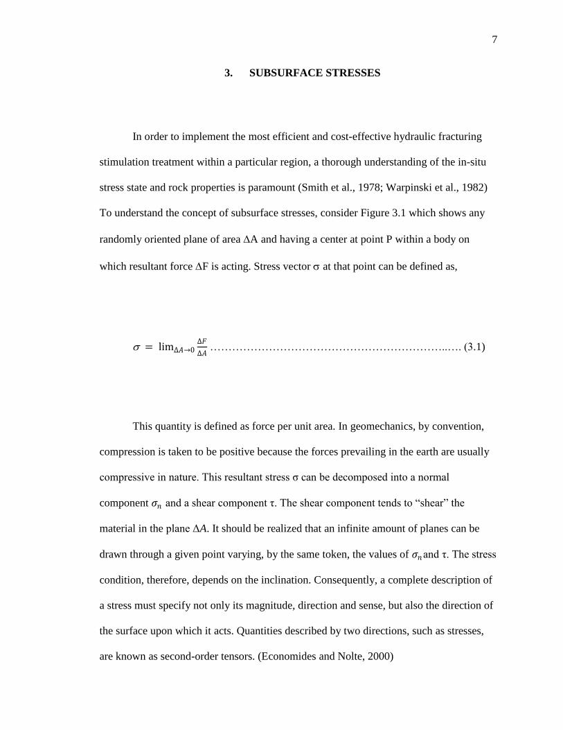
To understand the concept of subsurface stresses, consider Figure 3.1 which shows any

randomly oriented plane of area A and having a center at point P within a body on

which resultant force F is acting. Stress vector at that point can be defined as,

= lim∆𝐴→0∆𝐹

∆𝐴 ………………………………………………………..…. (3.1)

This quantity is defined as force per unit area. In geomechanics, by convention,

compression is taken to be positive because the forces prevailing in the earth are usually

compressive in nature. This resultant stress σ can be decomposed into a normal

component 𝜎𝑛 and a shear component τ. The shear component tends to “shear” the

material in the plane ΔA. It should be realized that an infinite amount of planes can be

drawn through a given point varying, by the same token, the values of 𝜎𝑛and τ. The stress

condition, therefore, depends on the inclination. Consequently, a complete description of

a stress must specify not only its magnitude, direction and sense, but also the direction of

the surface upon which it acts. Quantities described by two directions, such as stresses,

are known as second-order tensors. (Economides and Nolte, 2000)

8

Figure 3.1.Force F acting on a plane at point P having an area A (Economides and

Nolte, 2000)

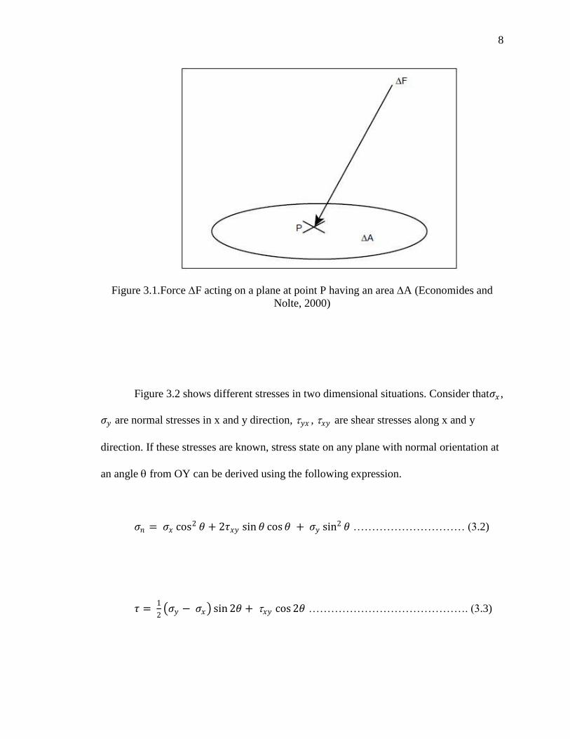
Figure 3.2 shows different stresses in two dimensional situations. Consider that𝜎𝑥 ,

𝜎𝑦 are normal stresses in x and y direction, 𝑦𝑥 , 𝑥𝑦 are shear stresses along x and y

direction. If these stresses are known, stress state on any plane with normal orientation at

an angle from OY can be derived using the following expression.

𝜎𝑛 = 𝜎𝑥 cos2 𝜃 + 2𝜏𝑥𝑦 sin 𝜃 cos 𝜃 + 𝜎𝑦 sin2 𝜃 ………………………… (3.2)

𝜏 = 1

2 𝜎𝑦 − 𝜎𝑥 sin 2𝜃 + 𝑥𝑦 cos 2𝜃 ……………………………………. (3.3)

9

Figure 3.2.Normal and Shear stresses acting in 2-D

(Economides and Nolte, 2000)

These expressions are obtained by writing equilibrium equations of the forces

along the 𝜎𝑛 and τ directions, respectively. The moment equilibrium implies that 𝑥𝑦 is

equal to𝑦𝑥 . There always exist two perpendicular orientations of ΔA for which the shear

stress components vanish; these are referred to as the principal planes. The normal

stresses associated with these planes are referred to as the principal stresses. In two

dimensions, expressions for these principal stresses can be found by setting τ = 0 in

Equation (3.3) or, because they are the minimum and maximum values of the normal

stresses, by taking the derivative of Equation (3.2) with respect to the angle θ and setting

10

it equal to zero. Either case obtains the following expression for the value of θ for which

the shear stress vanishes:

𝜃 = 1

2tan−1

2𝑥𝑦

𝜎𝑦− 𝜎𝑥 ………………………………………………………… (3.4)

And two principal stress components 𝜎1, 𝜎2 are,

𝜎1 = 1

2 𝜎𝑦 + 𝜎𝑥 + 𝜏2

𝑥𝑦 + 1

4 𝜎𝑦 − 𝜎𝑥

2

2

……………………………... (3.5)

𝜎2 = 1

2 𝜎𝑦 + 𝜎𝑥 − 𝜏2

𝑥𝑦 + 1

4 𝜎𝑦 − 𝜎𝑥

2

2

……………………………… (3.6)

If this concept is generalized to three dimensions, it can be shown that six

independent components of the stress (three normal and three shear components) are

needed to define the stress unambiguously. The stress vector for any direction of ΔA can

generally be found by writing equilibrium of force equations in various directions. Three

principal planes for which the shear stress components vanish and, therefore, the three

principal stresses exist. (Economides and Nolte, 2000)

11

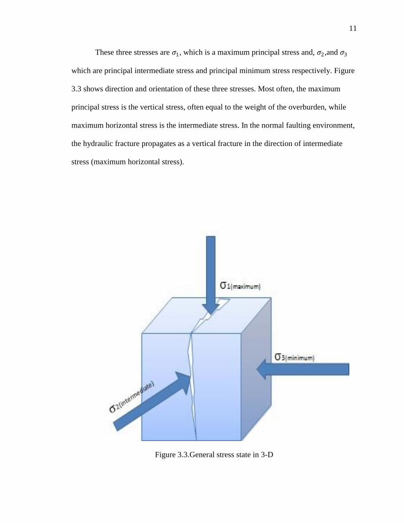
These three stresses are 𝜎1, which is a maximum principal stress and, 𝜎2,and 𝜎3

which are principal intermediate stress and principal minimum stress respectively. Figure

3.3 shows direction and orientation of these three stresses. Most often, the maximum

principal stress is the vertical stress, often equal to the weight of the overburden, while

maximum horizontal stress is the intermediate stress. In the normal faulting environment,

the hydraulic fracture propagates as a vertical fracture in the direction of intermediate

stress (maximum horizontal stress).

Figure 3.3.General stress state in 3-D

12

3.1 MOHR – COULOMB FAILURE ENVELOPE

After understanding the basics about the sub surface stresses, it is necessary to

understand their critical values at which rocks tend to fail. Failure criteria provide limits

to wellbore stresses and knowledge of rock strength is essential for accurate rock failure

analysis and to predict wellbore instability. They are derived from laboratory tests on

core samples, and can be typically divided into two broad categories: those that depend

on all three principal stresses, 𝜎1,𝜎2, 𝜎3 and those that neglect the effect of intermediate

principal stress 𝜎2 on failure. Two failure criteria are based on these categories: one

conventional triaxial criterion, the Mohr-Coulomb criterion, which ignores the influence

of the intermediate principal stress and is thus applicable to conventional triaxial test data

(𝜎1 > 𝜎2 = 𝜎3), and two “triaxial” criteria, i.e. the Modified Lade and the Drucker–

Prager, which consider the influence of the intermediate principal stress in polyaxial

strength tests (𝜎1 > 𝜎2 > 𝜎3). (Nawrocki, 2010)

The most commonly used technique is Mohr-Coulomb failure criterion. The

reason for its popularity include

1. Its rock failure parameters (cohesion, angle of internal friction, uniaxial

compressive strength) have physical meanings and the ranges of these parameters

have been established for many rocks.

2. It defines the failure plane orientation being the (𝜎1 − 𝜎3) plane, which has

always been observed in lab experiments.

3. It gives a quantitative measure of how far or how close a rock element is to shear

failure under a given applied loading condition. (Tran et al, 2010)

13

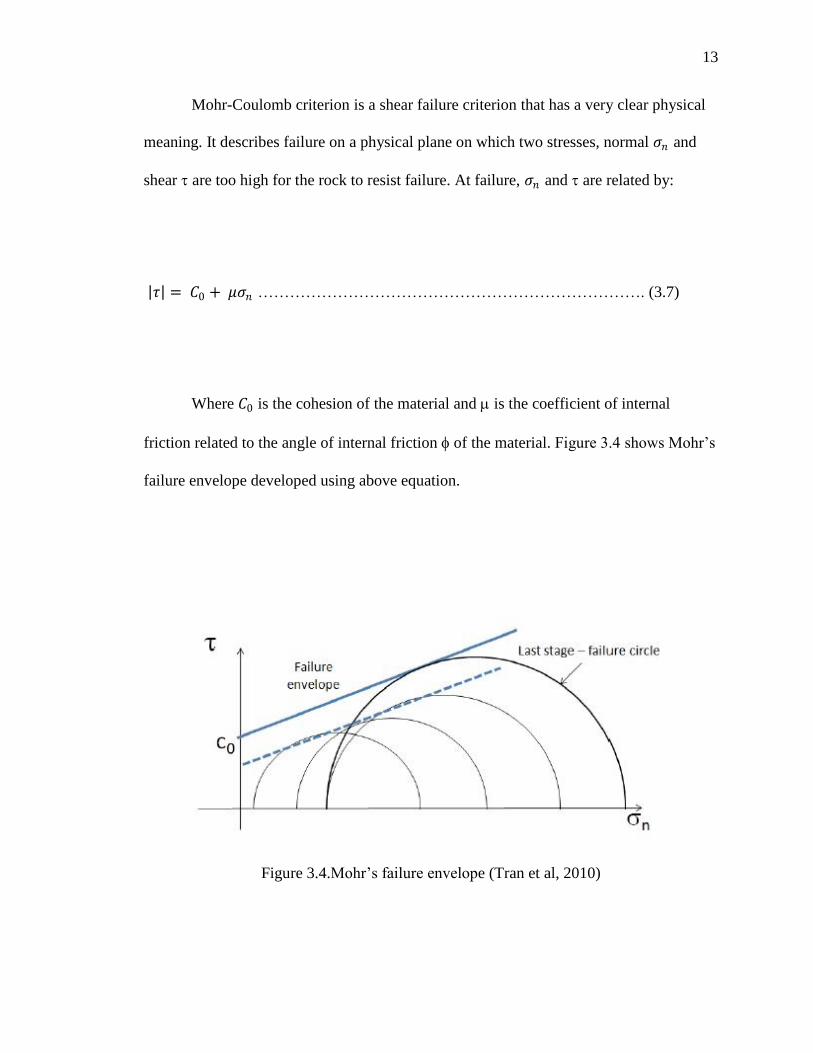
Mohr-Coulomb criterion is a shear failure criterion that has a very clear physical

meaning. It describes failure on a physical plane on which two stresses, normal 𝜎𝑛 and

shear are too high for the rock to resist failure. At failure, 𝜎𝑛 and are related by:

𝜏 = 𝐶0 + 𝜇𝜎𝑛 ………………………………………………………………. (3.7)

Where 𝐶0 is the cohesion of the material and is the coefficient of internal

friction related to the angle of internal friction of the material. Figure 3.4 shows Mohr‟s

failure envelope developed using above equation.

Figure 3.4.Mohr‟s failure envelope (Tran et al, 2010)

14

3.2 IN-SITU STRESS DETERMINATION

A reservoir rock, deposited in a sedimentary basin, is subjected to a certain

amount of pressure from the overlying rock layers. The vertical stress magnitude, at a

specific depth, H, is given by

𝜎𝑣 = 𝜌ℎ 𝑔 𝑑𝐻𝐻

0 ……………………………………………………….. (3.8)

Here 𝜌 is the density of the overlying rock masses and g is the acceleration due to

gravity. (Economides and Nolte, 1989)

The value of this stress component can be easily obtained from the integration of

a density log. If such a log is unavailable, a rule of thumb of 1.0 to 1.1 psi/ft is generally a

good approximation for this vertical stress component.

The prediction of the horizontal stress is based on two fundamentally different

premises. These two premises are commonly confused because, for tectonically relaxed

areas, they predict approximately the same ratio of 1 3 between the effective horizontal

and vertical stresses. The first premise is that the rock is in a state of incipient faulting

(Hubbert and Willis, 1957). For this condition, the state of stress is defined by the failure

envelope, and is independent of the elastic properties of the rock. Poroelastic constant,

describes the efficiency of the formation fluid pressure in counteracting the total applied

stress. For failure is equal to one.

The second, and fundamentally different premise, assumes the horizontal stress

depends only on the elastic behavior of the rock and is independent of the failure

15

envelope or any tectonic activity. In a basin not subjected to tectonic deformations, the

horizontal stress components, within a specific lithology, will be the same in every

direction. Because adjacent sections of a formation layer will tend to expand laterally,

their net interaction is zero lateral displacement. Using stress-strain relationship it can be

shown that (Hubbert and Willis, 1957)

𝜎2 = 𝜎3 = 𝜗

1−𝜗 𝜎𝑣 − 𝛼𝑃 + 𝛼𝑃 ………………………………………… (3.9)

Therefore, in tectonically inactive areas, the effective horizontal stress is

approximately equal to one-third of the effective vertical overburden, assuming that =

0.25.The variation of Poisson‟s ratio between different lithologies can lead to abrupt steps

in horizontal stress variations with depth.

.

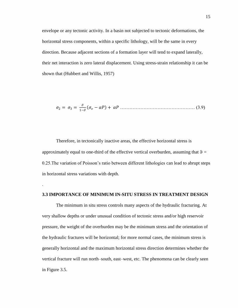
3.3 IMPORTANCE OF MINIMUM IN-SITU STRESS IN TREATMENT DESIGN

The minimum in situ stress controls many aspects of the hydraulic fracturing. At

very shallow depths or under unusual condition of tectonic stress and/or high reservoir

pressure, the weight of the overburden may be the minimum stress and the orientation of

the hydraulic fractures will be horizontal; for more normal cases, the minimum stress is

generally horizontal and the maximum horizontal stress direction determines whether the

vertical fracture will run north–south, east–west, etc. The phenomena can be clearly seen

in Figure 3.5.

16

Figure.3.5.Stress gradients varying over depths (Allen and Roberts, 1989)

Through its magnitude, the stress has a large bearing on material requirements,

pumping equipment, required for a treatment. Because the bottomhole pressure must

exceed the in-situ stress for fracture propagation, stress controls the required pumping

pressure that well tubulars must withstand and also controls the hydraulic horsepower

(hhp) required for the treatment. After fracturing, high stresses tend to crush the proppant

and reduce fracture conductivity; thus, the stress magnitude dominates the selection of

proppant type and largely controls post fracture conductivity. (Economides and Nolte,

2000)

17

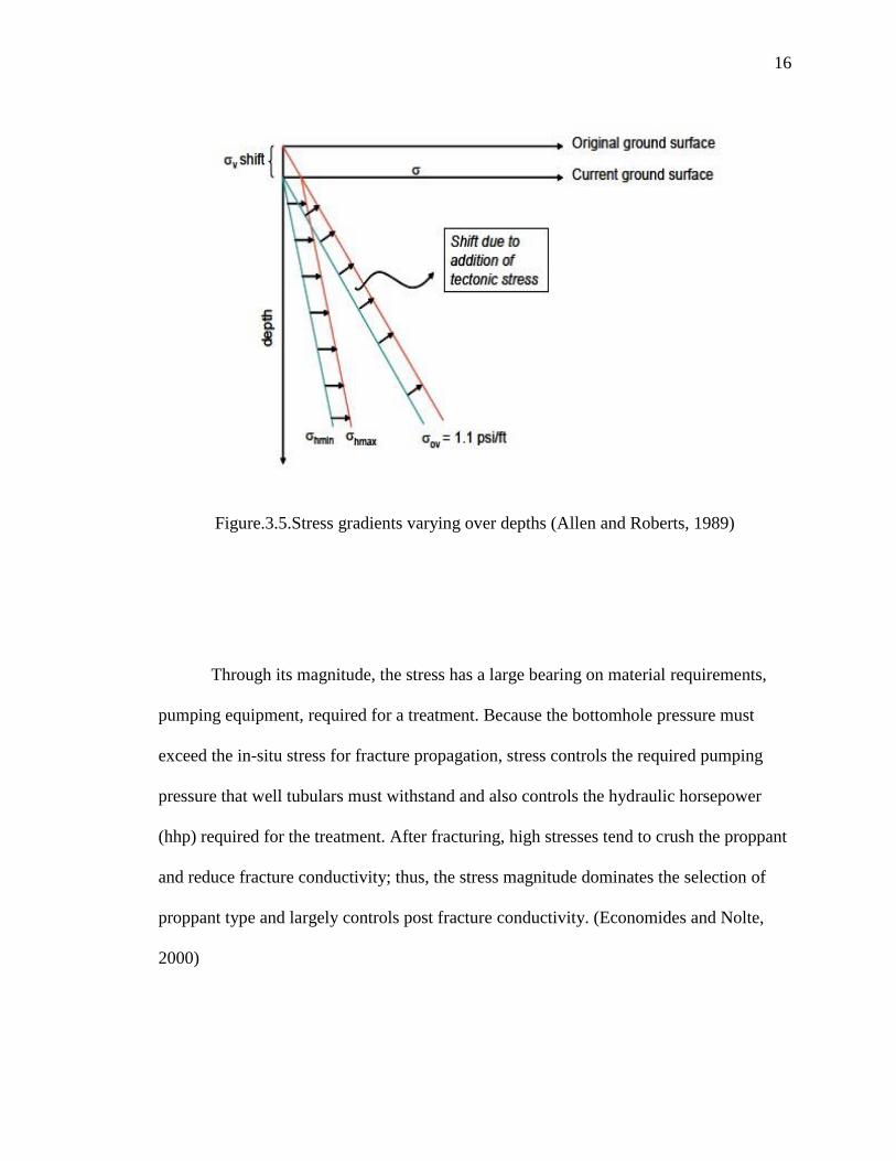
3.4 HYDRAULIC FRACTURING TREATMENT PRESSURE PROFILE

Figure 3.6 shows a generalized surface pressure plot for a hydraulic fracturing

treatment. This section discusses the various stages of the fracture treatment during

pumping and after shut-in, as shown in Figure 3.6.

Figure 3.6.Surface pressure plot for fracturing treatment (Allen and Roberts, 1989)

18

When fluid is pumped down the well bore at a pressure greater than regional

stresses, it results in formation break down. The fluid used for breaking down the

formation is called pad fluid and the entire stage is called pad stage. Because the fluid has

no space to escape, it exerts pressure on well bore walls. This results in pressure rise in

the beginning of the pad stage. The occurrence of breakdown is often seen on the surface

as a peak in the pressure plot. Breakdown occurs when hydraulic pressure exceeds the

compressive stresses at the borehole wall. Stress concentration results when a piece of

rock is removed from a rock matrix, while the regional rock matrix carries the same

matrix load and thus the rock at bore hole wall faces greater compressive stresses. After

the breakdown has occurred, pad fluid starts to leak off into the formation. If the injection

of pad fluid is continued further, the fracture tends to grow in width as well as length, as

the fluid pressure in the fracture works against the elasticity of the rock material.

After sufficient pad fluid is injected into the formation, pad stage ends and

proppant stage starts. In proppant stage, slurry consisting of a fluid blended with sand or

bauxite and some additives is injected down hole at a pressure sufficient to hold fracture

open. Here sand acts as a proppant. Slurry is injected into the formation with increasing

proppant concentration. Slurry stage is designed in such a way that, it will reach the

fracture tip as soon as all the pad fluid has leaked off in to the formation. Slurry gets

dehydrated gradually by leaking slurry fluid to the formation, as it moves forward

through the fracture and the stages are designed to have a uniform sand concentration

along the fracture at the end of pumping. Formation pore pressure gradually increases

during the treatment as more and more fluid is lost to the formation. This gradual increase

in pressure, referred to as an extension pressure can be seen during slurry stage in Figure

19

3.6. If the injection pressure is kept above extension pressure, fracture will tend to grow

in length and width. If the pressure inside the fracture is below extension pressure, but

above closure pressure, fracture will be held open but it will not propagate. Proppant

placement results in increase in fracture half length, width and height.

Pumps are shut down as soon as final stage of proppant is pumped down hole.

When pumping has stopped, there is a sudden in pressure versus time plot. The pumping

pressure at the instant of pump shut down is called an instantaneous shut-in pressure

(ISIP). Because fracture cannot close instantly upon pump shut-down, ISIP is generally

taken as an upper bound on the value for closure stress. (Jones and Britt, 2009) A Sudden

drop in pressure after pump shut down is a result of the fact that tubing friction losses

occur inside the tubing.

The pressure fall off after the ISIP, follows a gradual decline. The decline

continues until there is a break or an inflection point. This inflection point indicates a

change in linear flow behavior and is taken to indicate fracture closing. Generally this

value is taken to be value for closure stress.

Net pressure is the difference between fracture closure pressure and fracture

extension pressure. Net fracture pressure acts against the elasticity, or Young's modulus,

of the rock to open the fracture wider. During the fracture job, the net fracture pressure

can be used as an indicator of fracture extension. The Nolte – Smith plot is a log-log

representation of net pressure versus time or volume pumped which provides information

regarding fracture geometry and fracture propagation during a designing phase as well as

during actual treatment.

20

Accurate determination of closure stress is important because it is required in

calculation of net treating pressure. (Figure 3.6) Erroneous calculation of the closure

stress results in miscalculation of net pressure which leads to misinterpretation of critical

fracture design parameters such as fracture height, width, half length and fracture

geometry.

Additionally proppant conductivity depends largely upon the closure stress.

Different proppants show varying response as the closure stress increases. Fracture

roughness increases as the closure stress increases. Although fracture roughness is

neglected in many hydraulic fracturing models, there are situations where fracture

roughness is an important parameter. (van Dam et al. 1999)

There are different tests to calculate the closure stress. These tests will be

discussed in the next section.

21

4. HYDRAULIC FRACTURING PRESSURE TESTS AND THEIR

ANALYSES

4.1 HYDRAULIC FRACTURING PRESSURE TESTS

It is well established practice in oil and gas industry to determine different

fracturing parameters using different field pressure tests. These tests are carried out to

determine fracture closure pressure, fracture extension pressure, fluid leak off coefficient,

fracture geometry, efficiency, height and different elastic properties measured in-situ.

(Thompson and Church, 1993) These tests include;

1. Pump in/ flowback tests

2. Pump in/ decline tests

3. Step rate test

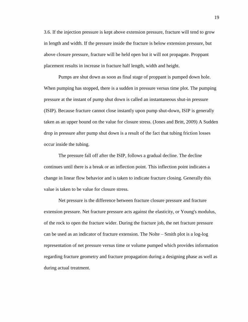
Figure 4.1 shows a pressure and flow rate behavior for an idealized pump in/

flowback test. Briefly, this procedure uses consists of injecting a volume of fluid at a

sufficient rate to initiate or open a fracture in the formation. After the injection, the well

is backflowed at an appropriate constant rate (e.g., through a surface choke) that varies

for different formations. In the desired range of flowback rates (e.g., one-quarter of the

injection rate), a plot of pressure vs. flowback time will exhibit a characteristic reversal of

curvature (i.e., increasing rate of decline) when the fracture closes. (Nolte and Smith,

1981)

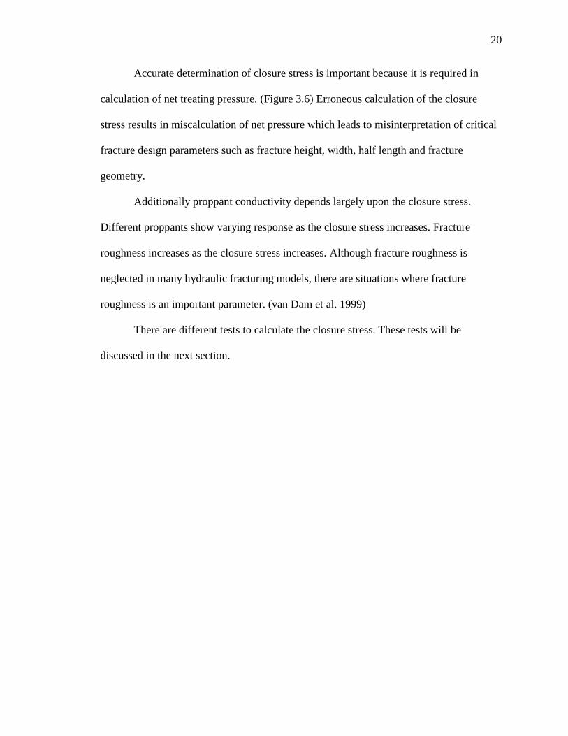
Figure 4.2 shows the influence of different flowback rates on a pump in flowback

test. Figure 4.3 shows a pump in/flowback test where closure stress is clearly evident

from the change of inflection during flowback.

22

Figure 4.1.Idealized pump in/flowback test (Soliman and Daneshi, 1991)

Figure 4.2.Pump in/flowback test showing effects of different rates

(Nolte, 1988)

23

The increasing rate of pressure decline, for the post closure period, results from

fluid flow through the pinched fracture width (i.e., induced fluid choking) in the near-

wellbore region induced by fluid flowback. The characteristic “lazy-S” signature

exhibited by the pressure during the flowback period is in contrast to the multiple

inflections commonly observed with the shut-in decline test. Therefore, the flowback test

provides a more objective indication of closure relative to the decline test. (Economides

and Nolte, 1989) however they are difficult to conduct because they are sensitive to how

flowback is conducted. (Figure 4.2)

Figure 4.3.Pump in/flowback test (Nolte, 1988)

24

Pump in decline pressure testing is commonly employed. In these tests a volume

of fluid is pumped into the formation at a constant rate and the well then shut in. Figure

4.4 shows pressure response for a typical pump in decline test. One example of pump in

test is a microfrac test. This test is usually conducted by perforating small interval (1 to 2

ft) in either permeable formation or in bounding shales to develop an in situ stress profile

with depth.

Small volume (0.5 to 1 bbl) of completion fluid is injected at 18 to 1 4 bbl/min. By

injecting such a small volume it is accepted that ISIP is a good approximation for closure

stress. For a better approximation of a closure stress, this test must be repeated several

times. Generally multiple tests tend to reduce any influence of wellbore and rock strength

because fracture is no longer being extended, but only reopened. ISIP is always an upper

bound on closure stress because fracture cannot close instantly as soon as pumping is

stopped. Therefore picking an ISIP value and making use of this value should be done

with care. A change in slope indicates that the fracture is closing. (Jones and Britt, 2009)

Figure 4.5 shows determination of closure stress from a decline part of the pressure

response shown in Figure 4.4. As can be seen from Figure 4.5, change of slope (inflection

point) is taken as the closure pressure. There are different possibilities as to how pressure

will respond after the fracture has been closed.

25

Figure 4.4.A typical pump in/decline test (Warpinski et al, 1985)

Figure 4.5.Change of slope representing closure stress value for pump in/decline test

(Nolte, 1988)

26

A step rate test (SRT) is always conducted to determine fracture extension

pressure. Fluid is pumped at constant incrementally increasing rates, and the final

injection pressure recorded for each rate is plotted vs. pump rate as shown in Figure 4.6.

A typical test may include injection rates ranging from 0.25 to10 bbl/min. The stabilized

final pressure for each step rate is plotted vs. pump rate, and the breakpoint is observed as

fracture extension pressure (Figure 4.7). For best results, each rate should be maintained

for a fixed period of time (typically 1 to 2 minutes). Also because of very slow rates at

the beginning of the test, proper pumping equipment is required. If bottomhole pressure

gauges are not used, a reliable SRT can be performed by shutting down well after each

rate step and obtaining an ISIP.

Figure 4.6.Rate v/s time plot for a typical step rate (Nolte, 1988)

27

Figure 4.7.Pressure versus flow rate plot showing extension pressure

Hydraulic fracturing in water wells is not common. Although not many water

wells are hydraulically fractured, records show that some have been fractured over the

past many years. These wells are not fractured so as to place a conductive pathway for

the recovery of formation fluid, but are fractured so as to test the formation integrity.

These wells are generally fracture tested to determine stress state of the underlying rocks

or to measure hydraulic conductivity.

Two different sets of tests are performed on water wells to estimate stress

parameters. These tests are a hydrofrac test and a hydro jack test. (ASTM, D 4645 – 87)

28

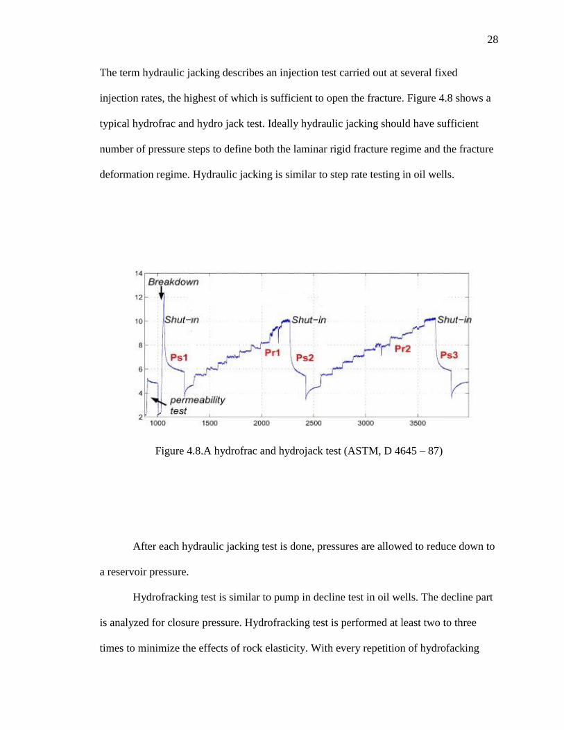
The term hydraulic jacking describes an injection test carried out at several fixed

injection rates, the highest of which is sufficient to open the fracture. Figure 4.8 shows a

typical hydrofrac and hydro jack test. Ideally hydraulic jacking should have sufficient

number of pressure steps to define both the laminar rigid fracture regime and the fracture

deformation regime. Hydraulic jacking is similar to step rate testing in oil wells.

Figure 4.8.A hydrofrac and hydrojack test (ASTM, D 4645 – 87)

After each hydraulic jacking test is done, pressures are allowed to reduce down to

a reservoir pressure.

Hydrofracking test is similar to pump in decline test in oil wells. The decline part

is analyzed for closure pressure. Hydrofracking test is performed at least two to three

times to minimize the effects of rock elasticity. With every repetition of hydrofacking

29

test, if closure pressure value is repeated, then it is taken as the final value. In Figure 4.8,

hydrofracking test can seen after the initial permeability test. The closure pressure value

𝑃𝑠1 is determined using the hydrofrac test.

Unlike oil domain, hydraulic fracturing in water wells is done using only water.

There are no proppant stages. The main intention to fracture the formation is to test

formation with respect to in situ stress state of stress and formation toughness and

integrity. In situ stresses can be measured directly by flatjack methods or indirectly using

strain rosette system, provided the location is at surface or in close proximity to an

opening. The flat jack method consists of making a slot in an exposed surface and

restoring measurement points to their initial position by applying pressures through flat

jacks. Pressures required are in correspondence with the normal stresses acting on the slot

surface. (C. Souza Martins, L. Ribiero E. Sousa, 1987). At distances less than 100 ft (30

m) or less from the access point, in situ stresses can be measured by a variety of borehole

methods incorporating instruments such as borehole deformation gauge, the „door-

stopper‟ or the inclusion stressmeter. However stress field must often be determined at

considerably greater distances. Hence water wells are typically tested with hydrofrac and

hydrojack test.

4.2 FRACTURING PRESSURE ANALYSIS USING ANALYTICAL

TECHNIQUES

The pressure data obtained after the conducting the fracturing treatment is

analyzed to obtain critical fracturing parameters. Various graphical techniques are more

commonly used to analyze the data. Some of these include,

30

1. Pressure versus square root of time analysis

2. G-Function plot analysis

3. G-dP/dG plot analysis

The Pressure versus square root of time plot is obtained by plotting bottomhole

pressure on Y- axis and square root of time on X- axis. The time here corresponds to time

since the pumps have been shut down. In this plot, a tangent is fitted to the early fall-off

period, and then to the later time after the fracture closes. Change slope indicates fracture

is closing. Therefore the intersection of the two lines approximates the formation closure

stress. Along with fracture closure pressure, square root of time plot also gives important

insights about exact closure time, fracture fluid efficiency and instantaneous shut in

pressure (ISIP). Figure 4.9 shows an example of pressure versus square root of time plot.

Here tangents are drawn whenever there is change in trend of curve and intersection of

tangents is taken as closure pressure value.

G- Function plot is somewhat superior to square root of time plot. G-Function plot

uses more precise relationship between pressure versus time compared to square root of

time plot. In G-Function plot, shown in Figure 4.10, derivative of G-Function is plotted

against the time. When derivative of G-Function is plotted against the time, it provides an

important information about fracture extension after shut-in, closure pressure and

pressure dependant leak-off. (Castillo, 1987) The G-Function plot finds its best

application in case of high permeability reservoirs where decline after pump shut off is

fast and it is difficult to observe sharp breaks in decline.

31

Figure 4.9.An example of square root of time plot analysis

Figure 4.10.An example of G-function plot analysis

32

G-dP/dG plot is generated by taking the derivative of pressure with respect to G-

Function (dp/dg) and plotting dp/dg as a function of the G-Function.(Baree and

Mukherjee, 1996) This method provides an accurate determination of magnitude of

pressure dependant leak off. As shown in Figure 4.11, second derivative pressure

response would exhibit a straight line and would be above or below the ideal line for non

ideal decline behavior like pressure dependent leakoff or height recession respectively.

Figure 4.11.An example of G-dP/dG plot analysis (Baree and Mukherjee, 1996)

33

4.3 SUBJECTIVITY ISSUES WITH ANALYTICAL METHODS

The analytical methods described in the previous section are widely used for the

determination of important fracturing parameters. However there may be a difficulty in

using these techniques because they are subjective to individual‟s interpretation. Here

closure stress is taken as the reference parameter to describe the subjectivity issues with

these techniques.

Consider Figure 4.12 which shows the square root of time plot for some pressure

fall-off data. The square root of time plot analysis was performed to obtain the closure

stress value. Tangents were drawn to the curve as shown in figure 4.12. The closure stress

obtained from this analysis was approximately 3428 psi.

Figure 4.12.Square root of time plot analysis showing Pc of 3428 psi

34

Now, the same set of data was analyzed second time using the same technique of

square root of time plot analysis. The only difference was that the tangents were fitted

differently compared to previous analysis, placing one tangent more along the late time

data. Figure 4.13 summarizes results for this analysis. In this case, closure stress obtained

for the same set of data was around 2847 psi, which was more than 500 psi smaller than

the previous analysis.

Figure 4.13.Square root of time plot analysis showing Pc of 2847 psi

As with the previous example one may also fit tangents with greater emphasis on

early time data. Figure 4.14 shows results obtained from this analysis. Here, for the same

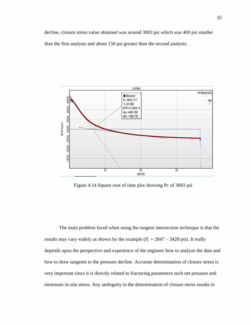
35

decline, closure stress value obtained was around 3003 psi which was 400 psi smaller

than the first analysis and about 150 psi greater than the second analysis.

Figure 4.14.Square root of time plot showing Pc of 3003 psi

The main problem faced when using the tangent intersection technique is that the

results may vary widely as shown by the example (𝑃𝑐 = 2847 – 3428 psi). It really

depends upon the perspective and experience of the engineer how to analyze the data and

how to draw tangents to the pressure decline. Accurate determination of closure stress is

very important since it is directly related to fracturing parameters such net pressure and

minimum in-situ stress. Any ambiguity in the determination of closure stress results in

36

erroneous calculations of net pressure and thus in wrong fracture geometry predictions

and fluid leak off coefficients. Closure stress is the single most important parameter for

the success of hydraulic fracturing treatment. Therefore above mentioned ambiguities in

the determination of closure stresses should be minimized by the introduction of more

definite method.

37

5. SQAURE ROOT OF TIME PLOT ANALYSIS FOR WATER WELL AND

GAS WELL

Two wells were used in this study, including a water well in southwestern

Missouri and gas well from Canadian gas formations. This section discusses the tests and

square root of time plot analysis for these tests.

5.1 CU PROJECT EXPLORATORY WELL # 1 (WATER WELL)

The data for this study is gathered from a city utilities project well # 1 which is a

𝐶𝑂2 sequestration project. When injecting 𝐶𝑂2 into a formation, it is mandatory to make

sure that the injected 𝐶𝑂2 does not break the formation. For this purpose it is important to

know critical reservoir parameters such as minimum in situ stress, formation break down

pressure. These parameters are estimated using hydraulic fracturing techniques.

Ten intervals from the bottom of the Reagan Sandstone through the Lamotte

formation were selected for pressure testing. These zones were tested according to ASTM

standards. The procedure uses two straddle packers set in an open hole to seal off the test

interval. With the packers anchored to the borehole wall, the formation test interval is

pressurized hydraulically by pumping at a constant flow rate. The general principle is to

affect hydrofracturing with a minute or so from the beginning of interval pressure rise.

Packer pressure must be maintained during testing to minimize leakoffs. As the rock

hydrofractures, a critical (or breakdown) pressure is reached. When pumping is stopped,

the pressure will drop to the instantaneous shut in pressure (ISIP). Repeated cycling of

38

the pressurization procedure using the same flow rate will yield the secondary breakdown

pressure (the pressure required to reopen a pre-existing fracture) and additional values of

the shut in pressure.

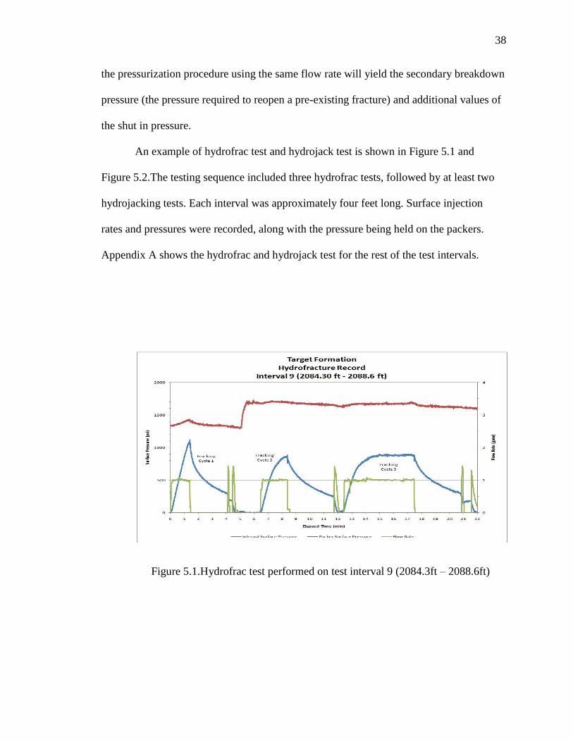
An example of hydrofrac test and hydrojack test is shown in Figure 5.1 and

Figure 5.2.The testing sequence included three hydrofrac tests, followed by at least two

hydrojacking tests. Each interval was approximately four feet long. Surface injection

rates and pressures were recorded, along with the pressure being held on the packers.

Appendix A shows the hydrofrac and hydrojack test for the rest of the test intervals.

Figure 5.1.Hydrofrac test performed on test interval 9 (2084.3ft – 2088.6ft)

39

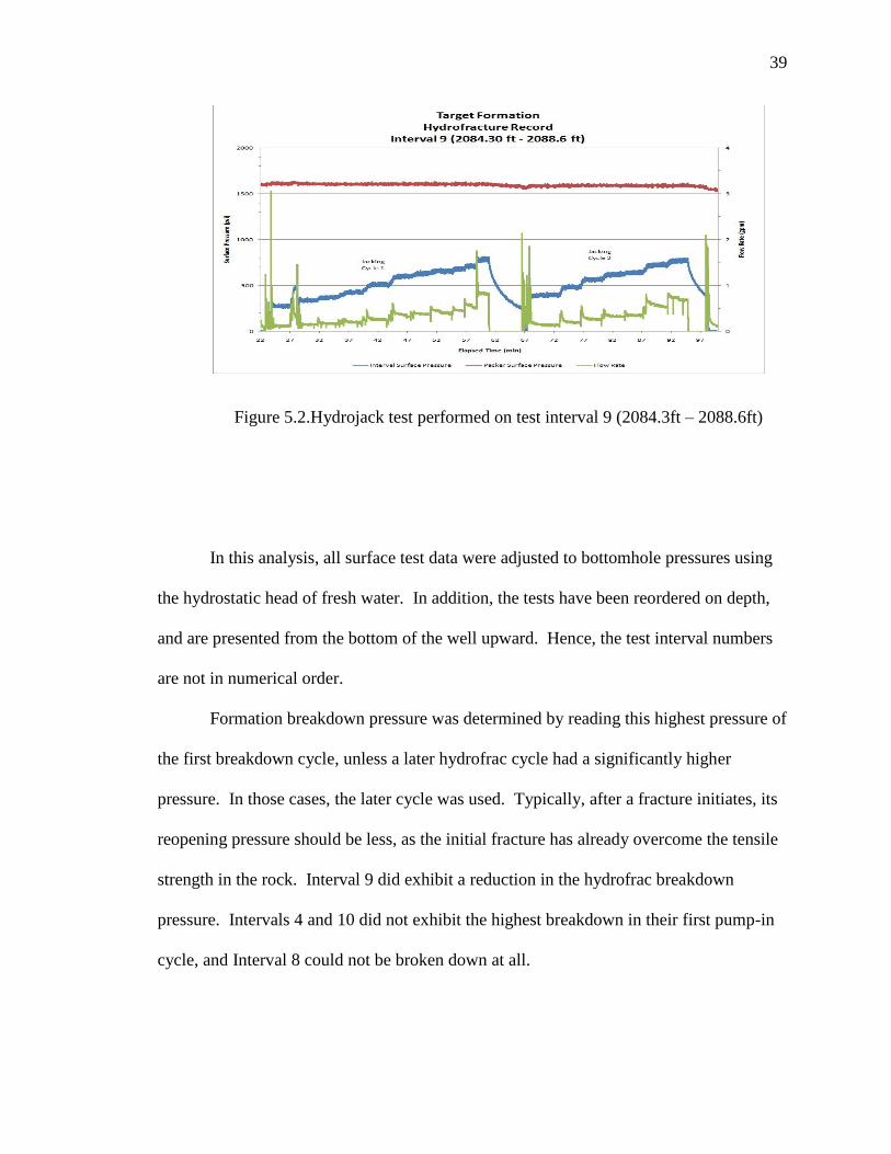
Figure 5.2.Hydrojack test performed on test interval 9 (2084.3ft – 2088.6ft)

In this analysis, all surface test data were adjusted to bottomhole pressures using

the hydrostatic head of fresh water. In addition, the tests have been reordered on depth,

and are presented from the bottom of the well upward. Hence, the test interval numbers

are not in numerical order.

Formation breakdown pressure was determined by reading this highest pressure of

the first breakdown cycle, unless a later hydrofrac cycle had a significantly higher

pressure. In those cases, the later cycle was used. Typically, after a fracture initiates, its

reopening pressure should be less, as the initial fracture has already overcome the tensile

strength in the rock. Interval 9 did exhibit a reduction in the hydrofrac breakdown

pressure. Intervals 4 and 10 did not exhibit the highest breakdown in their first pump-in

cycle, and Interval 8 could not be broken down at all.

40

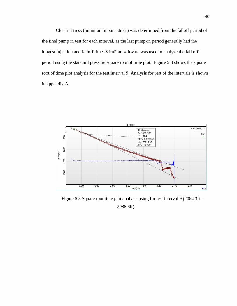
Closure stress (minimum in-situ stress) was determined from the falloff period of

the final pump in test for each interval, as the last pump-in period generally had the

longest injection and falloff time. StimPlan software was used to analyze the fall off

period using the standard pressure square root of time plot. Figure 5.3 shows the square

root of time plot analysis for the test interval 9. Analysis for rest of the intervals is shown

in appendix A.

Figure 5.3.Square root time plot analysis using for test interval 9 (2084.3ft –

2088.6ft)

41

5.2 CANADIAN GAS WELL # 2

Canadian gas well # 2 is a new producing well in an existing major gas field. The

well has been drilled and logged and preparations are being made to fracture stimulate the

well. This well is a planned Canadian formation completion with perforation at a depth of

1983 m – 1989 m. The objective is to design and place the optimum fracture stimulation

on this well to maximize both the initial potential and profitability of this new well.

Fracturing fluid planned for this job is water based cross linked gel and 20/40 Ottawa

sand. Prior to fracture stimulation job a series of pre fracture tests were conducted on the

well. Out of those, a stress test and a minifrac are taken for analysis purpose in this study.

Prior to mobilizing the fracture fleet, the well is perforated at 2020 meters and an in

situ stress and a step rate test were conducted to determine fracture closure pressure. For better

results, a stress test should be conducted with at least two step rate flow/flowback/decline tests

with very inefficient fluid. (Thompson and Church, 1993) Figure 5.4 shows a data plot for

stress test conducted on Canadian gas well # 2 at 2020 meters. It does not contain step rate

part as analysis is more focused on closure stress determination. As can be seen from the plot,

three successive pressurization cycles are carried out on the well, each followed by a pressure

decline part. The reason for conducting three pressurization cycles is to obtain repeated value

for closure stress and to minimize effect of elasticity of the rock. The second injection/decline

curve was taken for analysis to calculate the closure stress.

42

Figure 5.4.Data plot for stress test in Canadian gas well # 2

The decline part or pressure fall off period of the second pressurization cycle was

analyzed for closure stress calculation. The analysis was performed by constructing a square

root of time plot using StimPlan (Figure 5.5) Tangents were drawn to curves having different

slopes and intersection of tangents was taken as the value for closure stress.

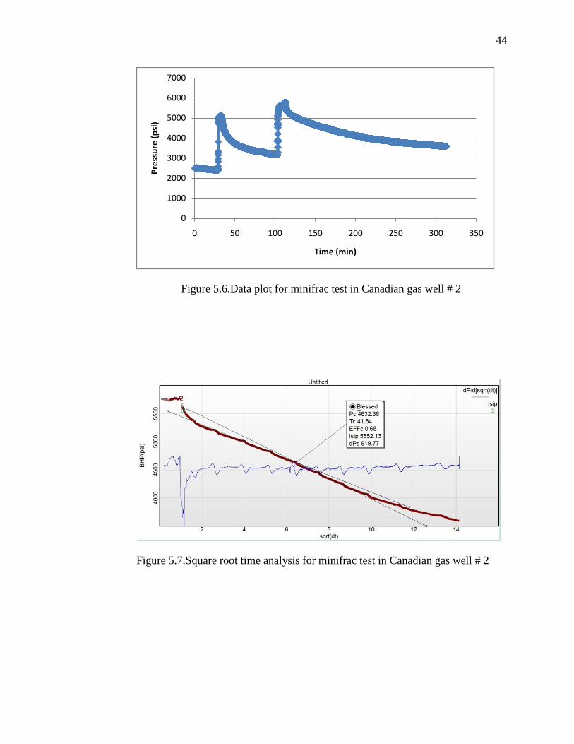
The gas well testing included a step rate test for fracture extension pressure, a

minifrac for fluid leak off coefficient, history matching, fracture closure pressures and for

redesigning the entire treatment. For the purpose of this study, only the minifrac was

considered and step rate for extension pressure was neglected. Figure 5.6 shows the data

plot for a minifrac conducted on well # 2.

0

1000

2000

3000

4000

5000

6000

7000

8000

0 20 40 60 80 100

Pre

ssu

re (

psi

)

Time (min)

43

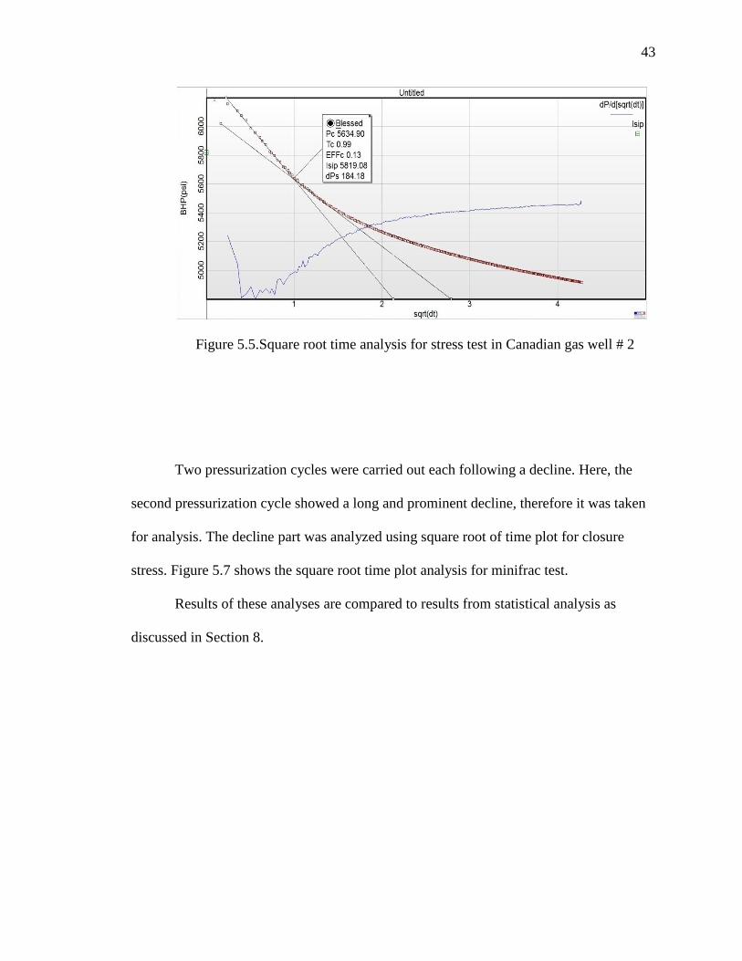
Figure 5.5.Square root time analysis for stress test in Canadian gas well # 2

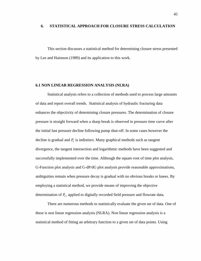
Two pressurization cycles were carried out each following a decline. Here, the

second pressurization cycle showed a long and prominent decline, therefore it was taken

for analysis. The decline part was analyzed using square root of time plot for closure

stress. Figure 5.7 shows the square root time plot analysis for minifrac test.

Results of these analyses are compared to results from statistical analysis as

discussed in Section 8.

44

Figure 5.6.Data plot for minifrac test in Canadian gas well # 2

Figure 5.7.Square root time analysis for minifrac test in Canadian gas well # 2

0

1000

2000

3000

4000

5000

6000

7000

0 50 100 150 200 250 300 350

Pre

ssu

re (

psi

)

Time (min)

45

6. STATISTICAL APPROACH FOR CLOSURE STRESS CALCULATION

This section discusses a statistical method for determining closure stress presented

by Lee and Haimson (1989) and its application to this work.

6.1 NON LINEAR REGRESSION ANALYSIS (NLRA)

Statistical analysis refers to a collection of methods used to process large amounts

of data and report overall trends. Statistical analysis of hydraulic fracturing data

enhances the objectivity of determining closure pressures. The determination of closure

pressure is straight forward when a sharp break is observed in pressure time curve after

the initial fast pressure decline following pump shut-off. In some cases however the

decline is gradual and 𝑃𝑐 is indistinct. Many graphical methods such as tangent

divergence, the tangent intersection and logarithmic methods have been suggested and

successfully implemented over the time. Although the square root of time plot analysis,

G-Function plot analysis and G-dP/dG plot analysis provide reasonable approximations,

ambiguities remain when pressure decay is gradual with no obvious breaks or knees. By

employing a statistical method, we provide means of improving the objective

determination of 𝑃𝑐 , applied to digitally recorded field pressure and flowrate data.

There are numerous methods to statistically evaluate the given set of data. One of

these is non linear regression analysis (NLRA). Non linear regression analysis is a

statistical method of fitting an arbitrary function to a given set of data points. Using

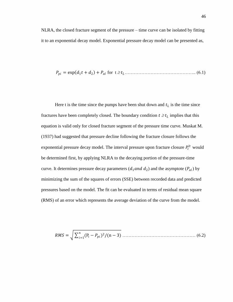
46

NLRA, the closed fracture segment of the pressure – time curve can be isolated by fitting

it to an exponential decay model. Exponential pressure decay model can be presented as,

𝑃𝑝𝑖 = exp 𝑑1𝑡 + 𝑑2 + 𝑃𝑎𝑙 for t 𝑡𝐿……………………………………….. (6.1)

Here t is the time since the pumps have been shut down and 𝑡𝐿 is the time since

fractures have been completely closed. The boundary condition 𝑡 𝑡𝐿 implies that this

equation is valid only for closed fracture segment of the pressure time curve. Muskat M.

(1937) had suggested that pressure decline following the fracture closure follows the

exponential pressure decay model. The interval pressure upon fracture closure 𝑃𝑐𝑙𝑡 would

be determined first, by applying NLRA to the decaying portion of the pressure-time

curve. It determines pressure decay parameters (𝑑1𝑎𝑛𝑑 𝑑2) and the asymptote (𝑃𝑎𝑙 ) by

minimizing the sum of the squares of errors (SSE) between recorded data and predicted

pressures based on the model. The fit can be evaluated in terms of residual mean square

(RMS) of an error which represents the average deviation of the curve from the model.

𝑅𝑀𝑆 = (Pi − 𝑃𝑝𝑖 )2/(n − 3)𝑛

𝑖=1 ………………………………………… (6.2)

47

In this equation, Pi is the actual pressure which is recorded on-field, 𝑃𝑝𝑖 is the

modeled pressure which is obtained using exponential pressure decay model and n is

simply number of the observation. This equation is known as RMS because it is square

root of mean of square of an error. Here error is simply the difference between observed

(actual) value for Pi and modeled value 𝑃𝑝𝑖 .

When these pressure decay parameters along with intial conditions and equations

for RMS and exponential pressure decay are fed to simulator, an iteration procedure is

invoked aimed at excluding the segment of the decaying pressure-time record before

fracture closure. Starting at the time of pump shut off (t = 0), data points will be removed

sequentially with each iteration. This fitting procedure would end when the decreasing

RMS value stabilizes. At this point it would be assumed all the pressure data belonging to

the open fracture time segment (t <𝑡𝑙) have been removed from the curve fitting process.

Figure 6.1 shows the process of curve fitting and determination closure stress using fitted

model over the actual data.

The largest pressure value of the fitted pressure-time curve (𝑃𝑐𝑙𝑡 ) is interpreted as

the level at which the induced fracture has completely closed, hence it is the lower limit

of the expected shut in pressure value. The extrapolated pressure level obtained by fitted

exponential curve at time t = 0 (𝑃𝑐𝑒𝑡 ) represents the pressure at which pure radial flow

would have commenced were the fracture to close instantaneously upon pump shut off. It

is thus the upper limit of the range of values within which 𝑃𝑐 is to be found. (Lee and

Haimson, 1989)

𝑃𝑐𝑙𝑡 <𝑃𝑐<𝑃𝑐

𝑒𝑡 ………………………………………………………………… (6.3)

48

Generally the value of 𝑃𝑐𝑒𝑡 yields more accurate approximation for the value of

closure stress (Lee and Haimson, 1989). Expected value of the closure stress should lie

within 100 psi of 𝑃𝑐𝑒𝑡 . Aamodt and Kuriyagawa have also recommended using 𝑃𝑐

𝑒𝑡 as

the closure pressure value.

Figure 6.1.Curve fitting process and RMS graph using NLRA (Lee and

Haimson, 1989)

6.2 SAS

All the statistical analysis of data for this study is done programmed a software

SAS. Before describing the actual work, this section provides basic information on SAS

and SAS programming.

49

SAS was developed in early 1970‟s at North Carolina State University. It was

originally intended for management and agricultural field experiments. It is now most

widely used statistical software. The name „SAS‟ used to be an abbreviation for

„Statistical Analysis System‟ however it is no longer an acronym for anything.

SAS system provides a powerful framework for statistical analysis. It has

extensive data manipulation capabilities to prepare for analytic and modeling work. It has

reporting tools for presenting results. Enterprise Guide (EG) enables to get answers

without having to write programs, through a point-and-click interface making selections

from a series of menus. As a benefit even for experienced SAS programmers, EG

provides a framework within which to organize the data, tasks, and results involved in

performing a statistical analysis, through the creation and maintenance of “projects”.

(Hallahan and Atkinson, USDA)

In SAS, we can create new projects, open existing projects, save projects, we can

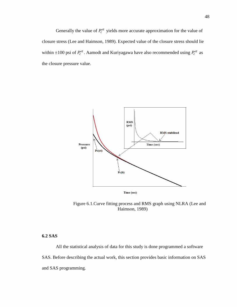
access data from outside. Enterprise Guide reads the data and brings it up in a data

viewer. Figure 6.2 shows a window that pops up after we create a new project. The empty

space in the middle is being provided for writing the program.

6.3 SAS PROGRAMMING

SAS as a programming language can be learned quickly and a user can begin

writing programs within hours of being introduced to SAS if there is the correct

information being taught.

50

Figure 6.2.SAS enterprise guide showing program window

SAS programming is easy to understand if the concept of „Step Boundaries‟ is

understood thoroughly. Step boundaries are denoted by „DATA‟ and „PROC‟ or

Procedure statements. SAS runs whatever code it finds within the step, processes the

data, then goes to the next step in the next DATA or PROC step, repeats the cycle within

the step, and so on until the end of the SAS job. When writing a SAS job, it should begin

with either DATA or PROC statement. (Clarence Jackson, CSQA)

A very important concept to understand is the computing cycle, which is simply „input

process - output‟.

Input is the start of any compute cycle. There must be something coming in to be

processed before any output can occur. Input for SAS programs can be from raw

data files, in stream cards or data lines, or SAS dataset/files. Input is what you

want to process.

51

Process is the part of the cycle that turns the input into something that can be

used, a very important part of the cycle.

Output is the part of the cycle that gives you what you need from the computer.

Every program requires input, processes the input, then returns the results as output.

SAS does that in so many different ways. It uses DATA step as an input and PROC step

as an output. (Clarence Jackson, CSQA)

6.3.1 SAS Programming Statements SAS programs are done by using SAS

statements that describe the action to be taken by SAS. SAS statements are delimited by

„;‟ or a semi-colon. This denotes then end of a statement segment. SAS is a free form

programming language, which means there are no rules regarding where on the line of

code statements need to be. Each statement contains a SAS keyword, at least one blank

between words, and a semi-colon. One can write SAS where one statement can span

multiple lines of code, which makes it possible to write code that is easy to read and

maintain.

SAS DATA steps usually create SAS datasets or datafiles from raw input data. SAS

uses the following keyword statements to perform the input process within the DATA

step:

INFILE statements defines the raw source file of data to be read into SAS

INPUT statements defines the location of fields on the record that will become

variables

CARDS/DATALINES tells SAS that data follows in the job stream. The „;‟ is

used to tell SAS to stop reading the data as data and start back to reading SAS

statements.

52

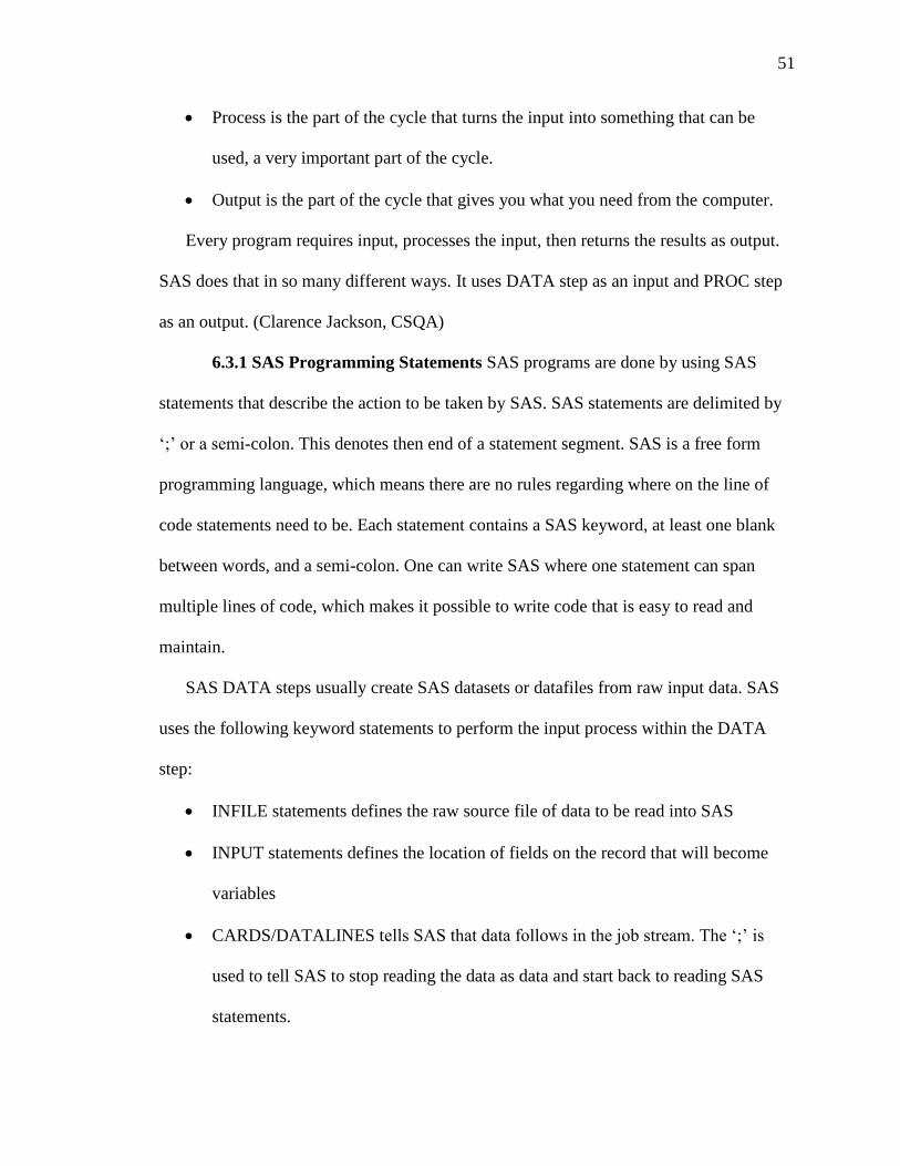
Figure 6.3 shows a simple program using all above defined statements. The first

step marked „A‟ consists of two statements; DATA and Input. The second step marked

„B‟ consists of one statement; Cards. Cards defines the input to the program. Step „C‟ is

Proc Print statement which is used to present output data in the tabular form or as a list.

Last step „C‟ is a Proc Corr statement. This statement is used when an output data needs

to be represented in some form of correlation.

Figure 6.3.A simple SAS program showing use of different statements

6.3.2 SAS Log File and Results File If SAS program stops running, SAS log

should be reviewed. The SAS Log report tells everything that SAS is doing, and will be a

source of feedback regarding the execution of the SAS program. It tells if an error is

being encountered, missed a record read, how many records were read and processed, and

other useful information. Figure 6.4 shows the log for the last program. If there were

53

errors, it would be „ERROR:‟ followed by the type of error encountered. One thing that

the log will not show you are logic errors. If the results are not what are intended, a log

file should be read to see what went on with your program, and should be compared with

what should be done with the program.

Figure 6.4.SAS log file for the sample program

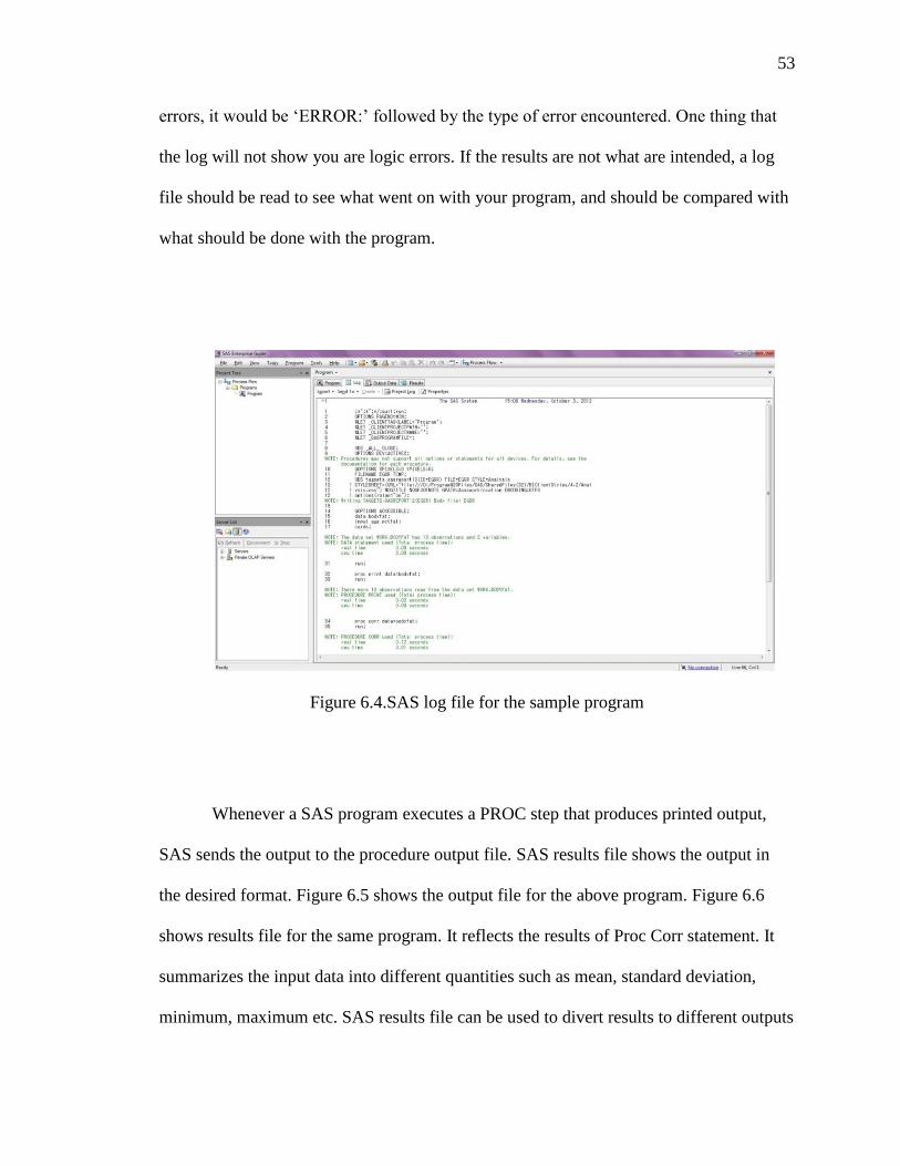
Whenever a SAS program executes a PROC step that produces printed output,

SAS sends the output to the procedure output file. SAS results file shows the output in

the desired format. Figure 6.5 shows the output file for the above program. Figure 6.6

shows results file for the same program. It reflects the results of Proc Corr statement. It

summarizes the input data into different quantities such as mean, standard deviation,

minimum, maximum etc. SAS results file can be used to divert results to different outputs

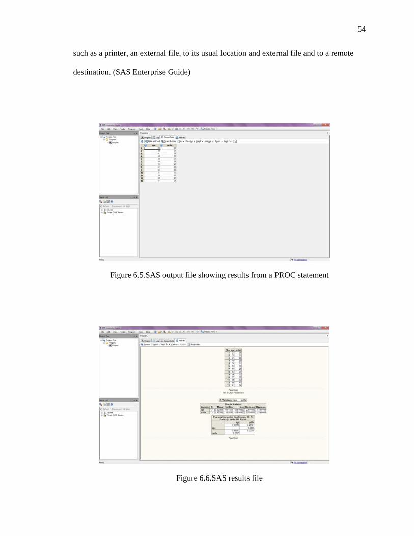
54

such as a printer, an external file, to its usual location and external file and to a remote

destination. (SAS Enterprise Guide)

Figure 6.5.SAS output file showing results from a PROC statement

Figure 6.6.SAS results file

55

7. STATISTICAL ANALYSIS OF THE DATA

7.1 THE ‘NLIN’ PROCEDURE

For statistical analysis of the non linear data used for this study, the „PROC

NLIN‟ procedure in SAS was extensively used. The NLIN procedure produces least

squares or weighted least squares estimates of the parameters of a nonlinear model.

Nonlinear models are more difficult to specify and estimate than linear models. Instead of

simply listing regressor (independent) variables, the regression expression must be

written, parameter names should be declared, and initial parameter values must be

supplied. Some models are difficult to fit, and there is no guarantee that the procedure

can fit the model successfully. For each nonlinear model to be analyzed, a model must be

specified (using a single dependent variable) and also, the names and starting values of

the parameters to be estimated must be specified.

Estimation of a nonlinear model is an iterative process. To begin this process the

NLIN procedure first examines the starting value specifications of the parameters. If a

grid of values is specified, PROC NLIN evaluates the residual sum of squares at each

combination of parameter values to determine the set of parameter values producing the

lowest residual sum of squares. These parameter values are used for the initial step of the

iteration. (SAS Online doc version)

Then PROC NLIN uses one of these five iterative methods:

1. steepest-descent or gradient method

2. Newton method

56

3. modified Gauss-Newton method

4. Marquardt method

5. multivariate secant or false position (DUD) method

These methods use derivatives or approximations to derivatives of the SSE (sum

of squares of the errors) with respect to the parameters to guide the search for the

parameters producing the smallest SSE.

Statistical analysis of the data used for this study used Gauss – Newton method

for non linear regression analysis. Figure 7.1 shows the program used for NLRA using

nlin procedure and Gauss – Newton method.

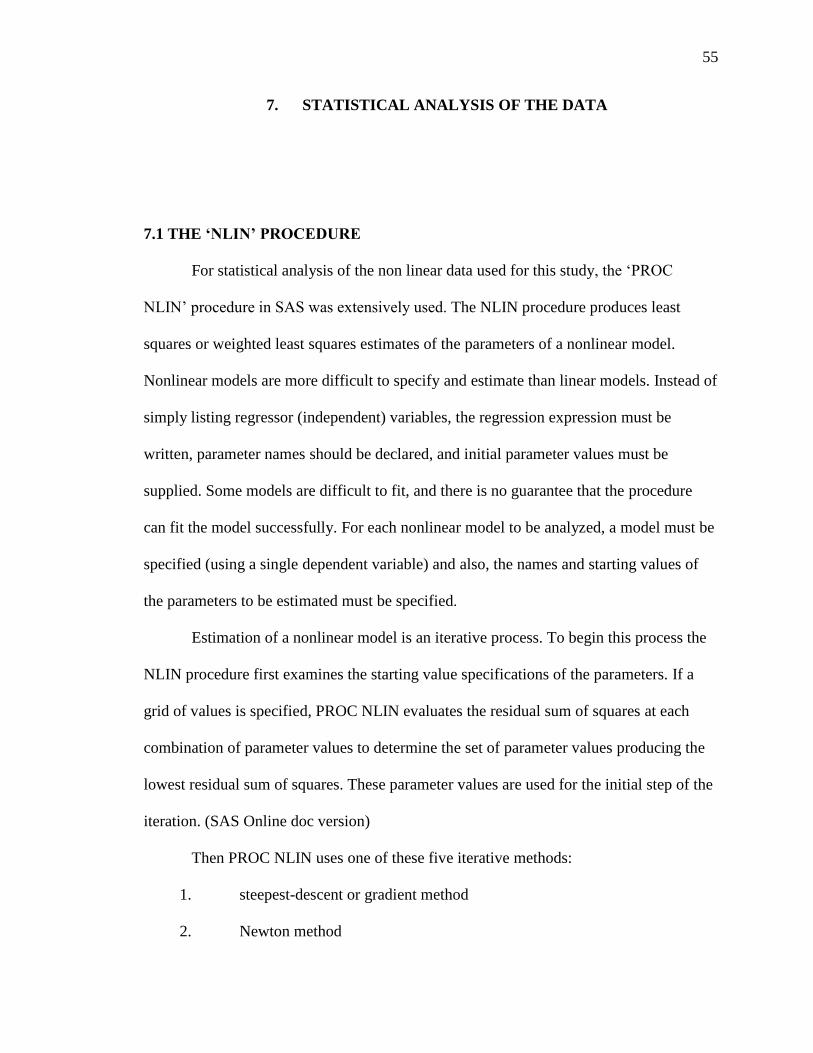
Figure 7.1.SAS program used for the study showing „nlin‟ procedure.

57

7.2. CU PROJECT EXPLORATORY WELL # 1 (WATER WELL)

A large amount of pressure data was collected when Lamotte and Reagan

sandstones were subjected to hydrofrac and hydrojack test cycles. As previously stated,

this zone of interest was divided into 10 intervals each approximately 4 feet tall and each

interval was pressure tested for breakdown pressures and extension pressures. For the

purpose of this study, each interval was analyzed statistically using NLRA for the closure

stress. Data corresponding to only the shut in part of the pressure – time curve was

selected. This is because closure stress can be calculated by analyzing only the decline

part of the pump in – fall off data. This data was then imported into SAS and proc nlin

procedure using Gauss – Newton method was implemented. Equation 6.1 was used to fit

exponential pressure decay model to the decline part of the data. As stated in section 7.1,

the proc nlin procedure requires initial parameters to start the iterative procedure.

Considering Equation 6.1, the initial parameters required to start iterations are 𝑑1, 𝑑2 and

C. Here 𝑑1, 𝑑2 are pressure decay constants. These parameters were calculated

independently for each test interval using sum of square of errors (SSE) between

recorded data and predicted pressures based on the model. The formation pressure was

selected as an asymptotic pressure for the calculation of initial parameters. The fit was

evaluated in terms of RMS using equation 6.2. An iteration procedure was invoked and

data points corresponding to open fracture segment were removed sequentially. The

fitting procedure ended when decreasing RMS values were stabilized. However, because

the program written to analyze the data was not so advanced that it would remove points

sequentially on its own, data points were remove manually and each time program was

run to do the iteration. Output from the simulator was analyzed each time to check if the

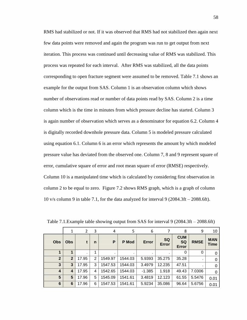
58

RMS had stabilized or not. If it was observed that RMS had not stabilized then again next

few data points were removed and again the program was run to get output from next

iteration. This process was continued until decreasing value of RMS was stabilized. This

process was repeated for each interval. After RMS was stabilized, all the data points

corresponding to open fracture segment were assumed to be removed. Table 7.1 shows an

example for the output from SAS. Column 1 is an observation column which shows

number of observations read or number of data points read by SAS. Column 2 is a time

column which is the time in minutes from which pressure decline has started. Column 3

is again number of observation which serves as a denominator for equation 6.2. Column 4

is digitally recorded downhole pressure data. Column 5 is modeled pressure calculated

using equation 6.1. Column 6 is an error which represents the amount by which modeled

pressure value has deviated from the observed one. Column 7, 8 and 9 represent square of

error, cumulative square of error and root mean square of error (RMSE) respectively.

Column 10 is a manipulated time which is calculated by considering first observation in

column 2 to be equal to zero. Figure 7.2 shows RMS graph, which is a graph of column

10 v/s column 9 in table 7.1, for the data analyzed for interval 9 (2084.3ft – 2088.6ft).

Table 7.1.Example table showing output from SAS for interval 9 (2084.3ft – 2088.6ft)

1 2 3 4 5 6 7 8 9 10

Obs Obs t n P P Mod Error SQ

Error

CUM SQ

Error RMSE

MAN Time

1 1 . 1 . . . . 0 0 0 2 2 17.95 2 1549.97 1544.03 5.9393 35.275 35.28 . 0 3 3 17.95 3 1547.53 1544.03 3.4979 12.235 47.51 . 0 4 4 17.95 4 1542.65 1544.03 -1.385 1.918 49.43 7.0306 0 5 5 17.96 5 1545.09 1541.61 3.4819 12.123 61.55 5.5476 0.01 6 6 17.96 6 1547.53 1541.61 5.9234 35.086 96.64 5.6756 0.01

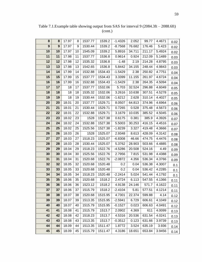
59

7

7 17.96 7 1542.65 1541.61 1.0405 1.083 97.72 4.9427

0.01 8 8 17.97 8 1537.77 1539.2 -1.4326 2.052 99.77 4.4671 0.02 9 9 17.97 9 1530.44 1539.2 -8.7568 76.682 176.46 5.423 0.02

10 10 17.97 10 1545.09 1539.2 5.8916 34.711 211.17 5.4924 0.02 11 11 17.98 11 1537.77 1536.8 0.9614 0.924 212.09 5.1489 0.03 12 12 17.98 12 1535.32 1536.8 -1.48 2.19 214.28 4.8795 0.03 13 13 17.98 13 1542.65 1536.8 5.8442 34.155 248.44 4.9843 0.03 14 14 17.99 14 1532.88 1534.43 -1.5429 2.38 250.82 4.7751 0.04 15 15 17.99 15 1537.77 1534.43 3.3399 11.155 261.97 4.6724 0.04 16 16 17.99 16 1532.88 1534.43 -1.5429 2.38 264.35 4.5094 0.04 17 17 18 17 1537.77 1532.06 5.703 32.524 296.88 4.6049 0.05 18 18 18 18 1535.32 1532.06 3.2616 10.638 307.51 4.5278 0.05 19 19 18 19 1530.44 1532.06 -1.6212 2.628 310.14 4.4027 0.05 20 20 18.01 20 1537.77 1529.71 8.0507 64.813 374.96 4.6964 0.06 21 21 18.01 21 1530.44 1529.71 0.7265 0.528 375.48 4.5673 0.06 22 22 18.01 22 1532.88 1529.71 3.1679 10.035 385.52 4.5045 0.06 23 23 18.02 23 1528 1527.38 0.6175 0.381 385.9 4.3926 0.07 24 24 18.02 24 1532.88 1527.38 5.5003 30.253 416.15 4.4516 0.07 25 25 18.02 25 1525.56 1527.38 -1.8239 3.327 419.48 4.3666 0.07 26 26 18.03 26 1528 1525.07 2.9348 8.613 428.09 4.3142 0.08 27 27 18.03 27 1518.23 1525.07 -6.8308 46.66 474.75 4.4476 0.08 28 28 18.03 28 1530.44 1525.07 5.3762 28.903 503.66 4.4885 0.08 29 29 18.04 29 1518.23 1522.76 -4.5286 20.508 524.16 4.49 0.09 30 30 18.04 30 1525.56 1522.76 2.7956 7.815 531.98 4.4388 0.09 31 31 18.04 31 1520.68 1522.76 -2.0872 4.356 536.34 4.3766 0.09 32 32 18.05 32 1520.68 1520.48 0.2 0.04 536.38 4.3007 0.1 33 33 18.05 33 1520.68 1520.48 0.2 0.04 536.42 4.2285 0.1 34 34 18.05 34 1518.23 1520.48 -2.2414 5.024 541.44 4.1792 0.1 35 35 18.06 35 1520.68 1518.2 2.4724 6.113 547.55 4.1366 0.11 36 36 18.06 36 1523.12 1518.2 4.9138 24.146 571.7 4.1622 0.11 37 37 18.06 37 1515.79 1518.2 -2.4104 5.81 577.51 4.1214 0.11 38 38 18.07 38 1520.68 1515.95 4.7301 22.374 599.88 4.14 0.12 39 39 18.07 39 1513.35 1515.95 -2.5941 6.729 606.61 4.1049 0.12 40 40 18.07 40 1515.79 1515.95 -0.1527 0.023 606.63 4.0491 0.12 41 41 18.08 41 1515.79 1513.7 2.0902 4.369 611 4.0099 0.13 42 42 18.08 42 1518.23 1513.7 4.5316 20.536 631.54 4.0241 0.13 43 43 18.08 43 1513.35 1513.7 -0.3512 0.123 631.66 3.9739 0.13 44 44 18.09 44 1513.35 1511.47 1.8772 3.524 635.19 3.936 0.14 45 45 18.09 45 1515.79 1511.47 4.3186 18.651 653.84 3.9456 0.14

Table 7.1.Example table showing output from SAS for interval 9 (2084.3ft – 2088.6ft)

(cont.)

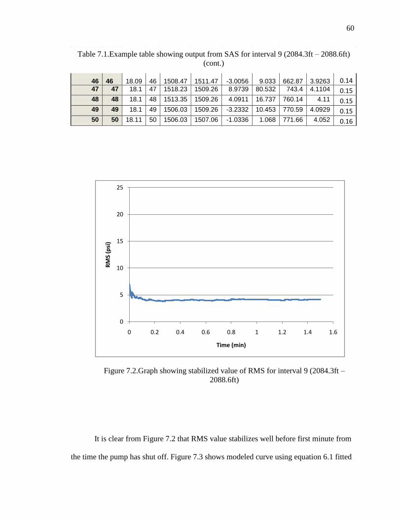
60

46

46

18.09

46

1508.47

1511.47

-3.0056

9.033

662.87

3.9263 0.14 47 47 18.1 47 1518.23 1509.26 8.9739 80.532 743.4 4.1104 0.15 48 48 18.1 48 1513.35 1509.26 4.0911 16.737 760.14 4.11 0.15 49 49 18.1 49 1506.03 1509.26 -3.2332 10.453 770.59 4.0929 0.15 50 50 18.11 50 1506.03 1507.06 -1.0336 1.068 771.66 4.052 0.16

Figure 7.2.Graph showing stabilized value of RMS for interval 9 (2084.3ft –

2088.6ft)

It is clear from Figure 7.2 that RMS value stabilizes well before first minute from

the time the pump has shut off. Figure 7.3 shows modeled curve using equation 6.1 fitted

0

5

10

15

20

25

0 0.2 0.4 0.6 0.8 1 1.2 1.4 1.6

RM

S (p

si)

Time (min)

Table 7.1.Example table showing output from SAS for interval 9 (2084.3ft – 2088.6ft)

(cont.)

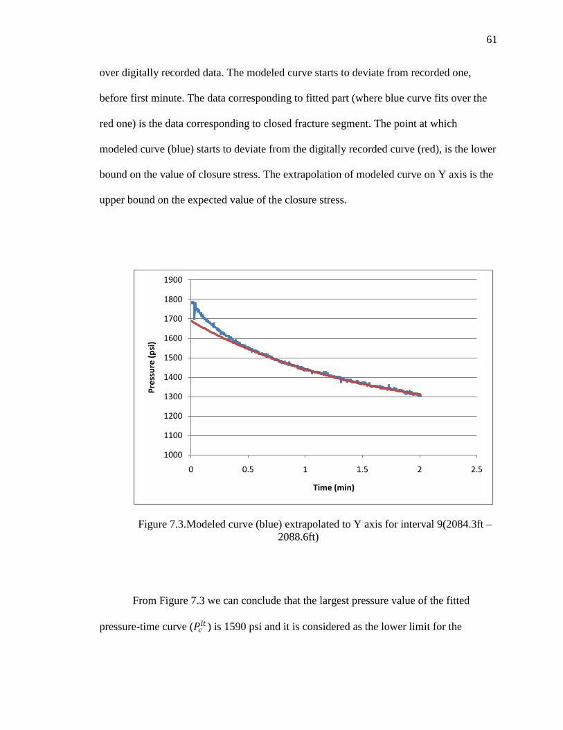
61

over digitally recorded data. The modeled curve starts to deviate from recorded one,

before first minute. The data corresponding to fitted part (where blue curve fits over the

red one) is the data corresponding to closed fracture segment. The point at which

modeled curve (blue) starts to deviate from the digitally recorded curve (red), is the lower

bound on the value of closure stress. The extrapolation of modeled curve on Y axis is the

upper bound on the expected value of the closure stress.

Figure 7.3.Modeled curve (blue) extrapolated to Y axis for interval 9(2084.3ft –

2088.6ft)

From Figure 7.3 we can conclude that the largest pressure value of the fitted

pressure-time curve (𝑃𝑐𝑙𝑡 ) is 1590 psi and it is considered as the lower limit for the

1000

1100

1200

1300

1400

1500

1600

1700

1800

1900

0 0.5 1 1.5 2 2.5

Pre

ssu

re (

psi

)

Time (min)

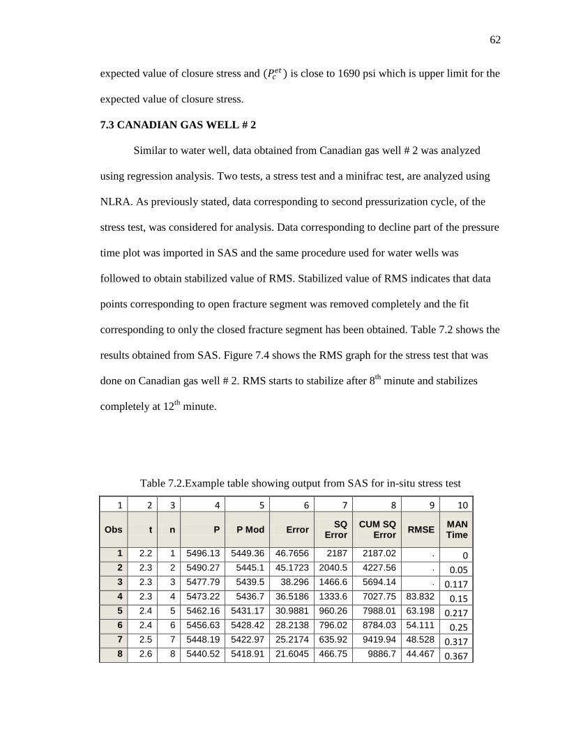
62

expected value of closure stress and (𝑃𝑐𝑒𝑡 ) is close to 1690 psi which is upper limit for the

expected value of closure stress.

7.3 CANADIAN GAS WELL # 2

Similar to water well, data obtained from Canadian gas well # 2 was analyzed

using regression analysis. Two tests, a stress test and a minifrac test, are analyzed using

NLRA. As previously stated, data corresponding to second pressurization cycle, of the

stress test, was considered for analysis. Data corresponding to decline part of the pressure

time plot was imported in SAS and the same procedure used for water wells was

followed to obtain stabilized value of RMS. Stabilized value of RMS indicates that data

points corresponding to open fracture segment was removed completely and the fit

corresponding to only the closed fracture segment has been obtained. Table 7.2 shows the

results obtained from SAS. Figure 7.4 shows the RMS graph for the stress test that was

done on Canadian gas well # 2. RMS starts to stabilize after 8th

minute and stabilizes

completely at 12th

minute.

Table 7.2.Example table showing output from SAS for in-situ stress test

1 2 3 4 5 6 7 8 9 10

Obs t n P P Mod Error SQ

Error CUM SQ

Error RMSE

MAN Time

1 2.2 1 5496.13 5449.36 46.7656 2187 2187.02 . 0 2 2.3 2 5490.27 5445.1 45.1723 2040.5 4227.56 . 0.05 3 2.3 3 5477.79 5439.5 38.296 1466.6 5694.14 . 0.117 4 2.3 4 5473.22 5436.7 36.5186 1333.6 7027.75 83.832 0.15 5 2.4 5 5462.16 5431.17 30.9881 960.26 7988.01 63.198 0.217 6 2.4 6 5456.63 5428.42 28.2138 796.02 8784.03 54.111 0.25 7 2.5 7 5448.19 5422.97 25.2174 635.92 9419.94 48.528 0.317 8 2.6 8 5440.52 5418.91 21.6045 466.75 9886.7 44.467 0.367

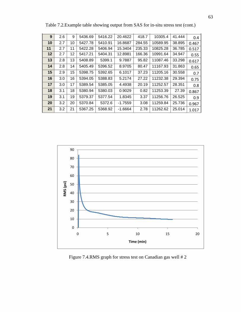
63

9 2.6 9 5436.69 5416.22 20.4622 418.7 10305.4 41.444 0.4 10 2.7 10 5427.78 5410.91 16.8687 284.55 10589.95 38.895 0.467

11 2.7 11 5422.28 5406.94 15.3404 235.33 10825.28 36.785 0.517 12 2.7 12 5417.21 5404.31 12.8981 166.36 10991.64 34.947 0.55 13 2.8 13 5408.89 5399.1 9.7887 95.82 11087.46 33.298 0.617 14 2.8 14 5405.49 5396.52 8.9705 80.47 11167.93 31.863 0.65 15 2.9 15 5398.75 5392.65 6.1017 37.23 11205.16 30.558 0.7 16 3.0 16 5394.05 5388.83 5.2174 27.22 11232.38 29.394 0.75 17 3.0 17 5389.54 5385.05 4.4938 20.19 11252.57 28.351 0.8 18 3.1 18 5380.94 5380.03 0.9029 0.82 11253.39 27.39 0.867 19 3.1 19 5379.37 5377.54 1.8345 3.37 11256.76 26.525 0.9 20 3.2 20 5370.84 5372.6 -1.7559 3.08 11259.84 25.736 0.967 21 3.2 21 5367.25 5368.92 -1.6664 2.78 11262.62 25.014 1.017

Figure 7.4.RMS graph for stress test on Canadian gas well # 2

0

10

20

30

40

50

60

70

80

90

0 5 10 15 20

RM

S (p

si)

Time (min)

Table 7.2.Example table showing output from SAS for in-situ stress test (cont.)

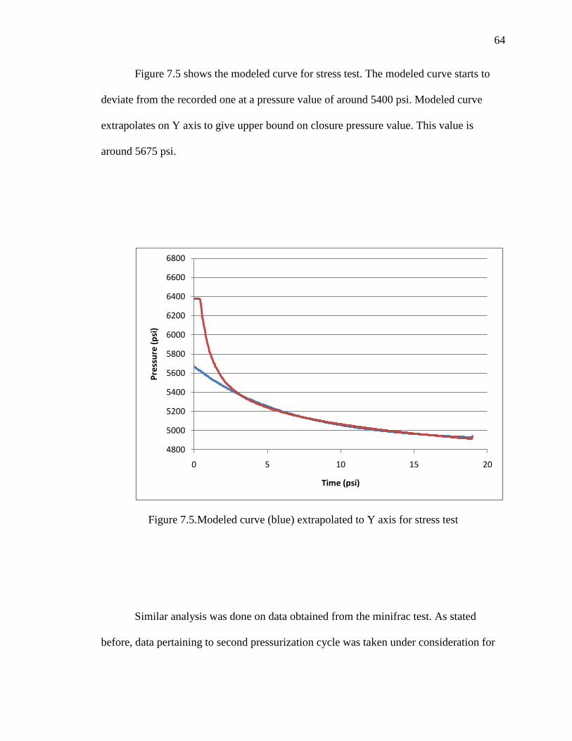
64

Figure 7.5 shows the modeled curve for stress test. The modeled curve starts to

deviate from the recorded one at a pressure value of around 5400 psi. Modeled curve

extrapolates on Y axis to give upper bound on closure pressure value. This value is

around 5675 psi.

Figure 7.5.Modeled curve (blue) extrapolated to Y axis for stress test

Similar analysis was done on data obtained from the minifrac test. As stated

before, data pertaining to second pressurization cycle was taken under consideration for

4800

5000

5200

5400

5600

5800

6000

6200

6400

6600

6800

0 5 10 15 20

Pre

ssu

re (

psi

)

Time (psi)

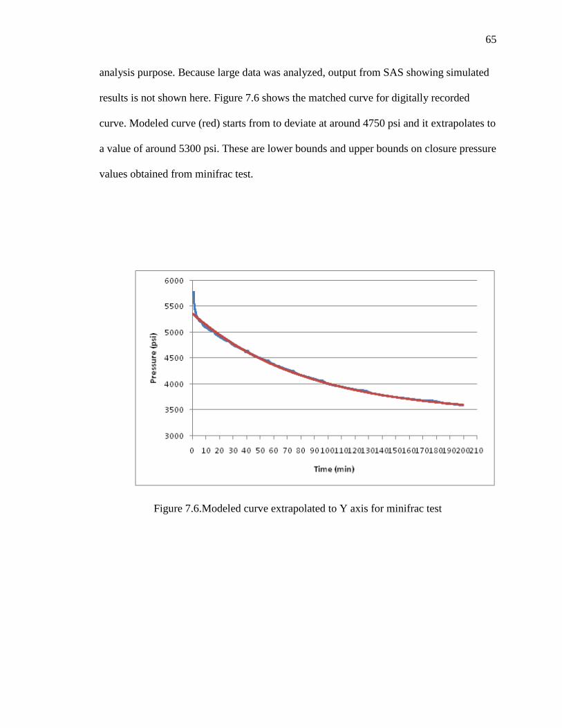
65

analysis purpose. Because large data was analyzed, output from SAS showing simulated

results is not shown here. Figure 7.6 shows the matched curve for digitally recorded

curve. Modeled curve (red) starts from to deviate at around 4750 psi and it extrapolates to

a value of around 5300 psi. These are lower bounds and upper bounds on closure pressure

values obtained from minifrac test.

Figure 7.6.Modeled curve extrapolated to Y axis for minifrac test

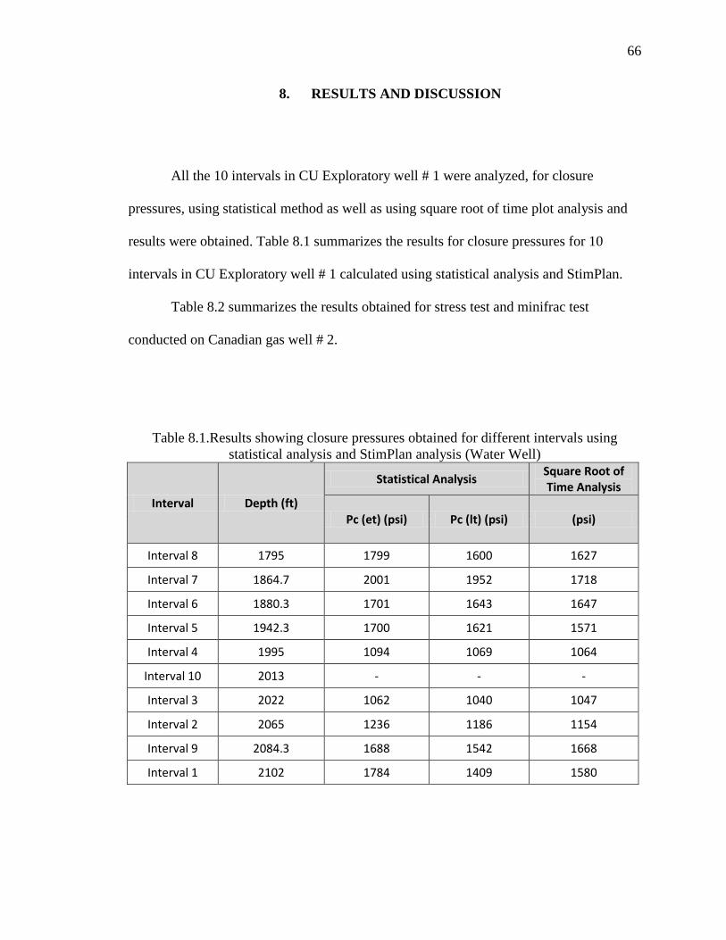
66

8. RESULTS AND DISCUSSION

All the 10 intervals in CU Exploratory well # 1 were analyzed, for closure

pressures, using statistical method as well as using square root of time plot analysis and

results were obtained. Table 8.1 summarizes the results for closure pressures for 10

intervals in CU Exploratory well # 1 calculated using statistical analysis and StimPlan.

Table 8.2 summarizes the results obtained for stress test and minifrac test

conducted on Canadian gas well # 2.

Table 8.1.Results showing closure pressures obtained for different intervals using

statistical analysis and StimPlan analysis (Water Well)

Interval Depth (ft)

Statistical Analysis Square Root of Time Analysis

Pc (et) (psi) Pc (lt) (psi) (psi)

Interval 8 1795 1799 1600 1627

Interval 7 1864.7 2001 1952 1718

Interval 6 1880.3 1701 1643 1647

Interval 5 1942.3 1700 1621 1571

Interval 4 1995 1094 1069 1064

Interval 10 2013 - - -

Interval 3 2022 1062 1040 1047

Interval 2 2065 1236 1186 1154

Interval 9 2084.3 1688 1542 1668

Interval 1 2102 1784 1409 1580

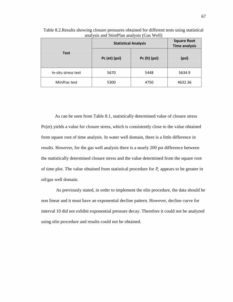
67

Table 8.2.Results showing closure pressures obtained for different tests using statistical

analysis and StimPlan analysis (Gas Well)

Test

Statistical Analysis Square Root

Time analysis

Pc (et) (psi) Pc (lt) (psi) (psi)

In-situ stress test 5670 5448 5634.9

Minifrac test 5300 4750 4632.36

As can be seen from Table 8.1, statistically determined value of closure stress

Pc(et) yields a value for closure stress, which is consistently close to the value obtained

from square root of time analysis. In water well domain, there is a little difference in

results. However, for the gas well analysis there is a nearly 200 psi difference between

the statistically determined closure stress and the value determined from the square root

of time plot. The value obtained from statistical procedure for 𝑃𝑐 appears to be greater in

oil/gas well domain.

As previously stated, in order to implement the nlin procedure, the data should be

non linear and it must have an exponential decline pattern. However, decline curve for

interval 10 did not exhibit exponential pressure decay. Therefore it could not be analyzed

using nlin procedure and results could not be obtained.

68

9. CONCLUSION

In this study, statistical analysis and it‟s applicability to determine closure stress

was studied. The study included a comparison of closure stress using a standard square

rot of time plot and a statistical approach in which Non Linear Regression Analysis was

carried out. The data used for this study was from the to CU project Exploratory Well #

1, which is a water well drilled in Lamotte and Reagan sandstone formations. The data

from Canadian gas well # 2 was also used for comparing the oil/ gas domain to the water

well domain.

In CU exploratory well, all the intervals showed good results using NLRA except

for interval 10, for which results could not be obtained because of non-exponential nature

of the decline. Closure pressures obtained for each interval was in a range of 100 psi of

the square root time analysis results. In Canadian gas well, NLRA results obtained for in-

situ stress test were in good agreement with the square root time analysis results,

indicating there is greater applicability for the statistical method in the oil/gas well

domain. For a minifrac test conducted in same formation, NLRA gave closure stress

value which was comparable with closure stress obtained from in-situ stress test.

However square root time analysis results for a minifrac test were ambiguous and were in

no close proximity of the results obtained from NLRA.

There are few limitations about the study. The program used for the analysis of

data was case specific. It was only built for an exponential pressure decay model. Also,

the method used here can be applied only for the determination of closure stress. Other

fracturing parameters such as fracture re-opening pressure, fracture extension pressure

69

could not be determined using this (exponential pressure decay) method. This does not

mean that statistical approach cannot be used for determining these parameters and

should be considered as a future work for this study. The approach taken in this study can

be taken as a reference and other methods can be applied to analyze the data statistically.

Further work is also recommended for developing the program which would do

successive iterations on its own for getting the best possible fit.

Statistical analysis is a handy tool for the objective determination of closure

stress. Along with all the graphical methods that are used in the industry today, statistical

analysis should be given an equal consideration as it can become a powerful method to

determine the closure stress objectively.

70

APPENDIX A

STIMPLAN ANALYSIS, DIGITALLY RECORDED CURVES AND MODELED

CURVES

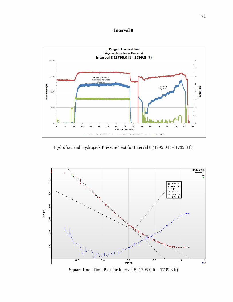
71

Interval 8

Hydrofrac and Hydrojack Pressure Test for Interval 8 (1795.0 ft – 1799.3 ft)

Square Root Time Plot for Interval 8 (1795.0 ft – 1799.3 ft)

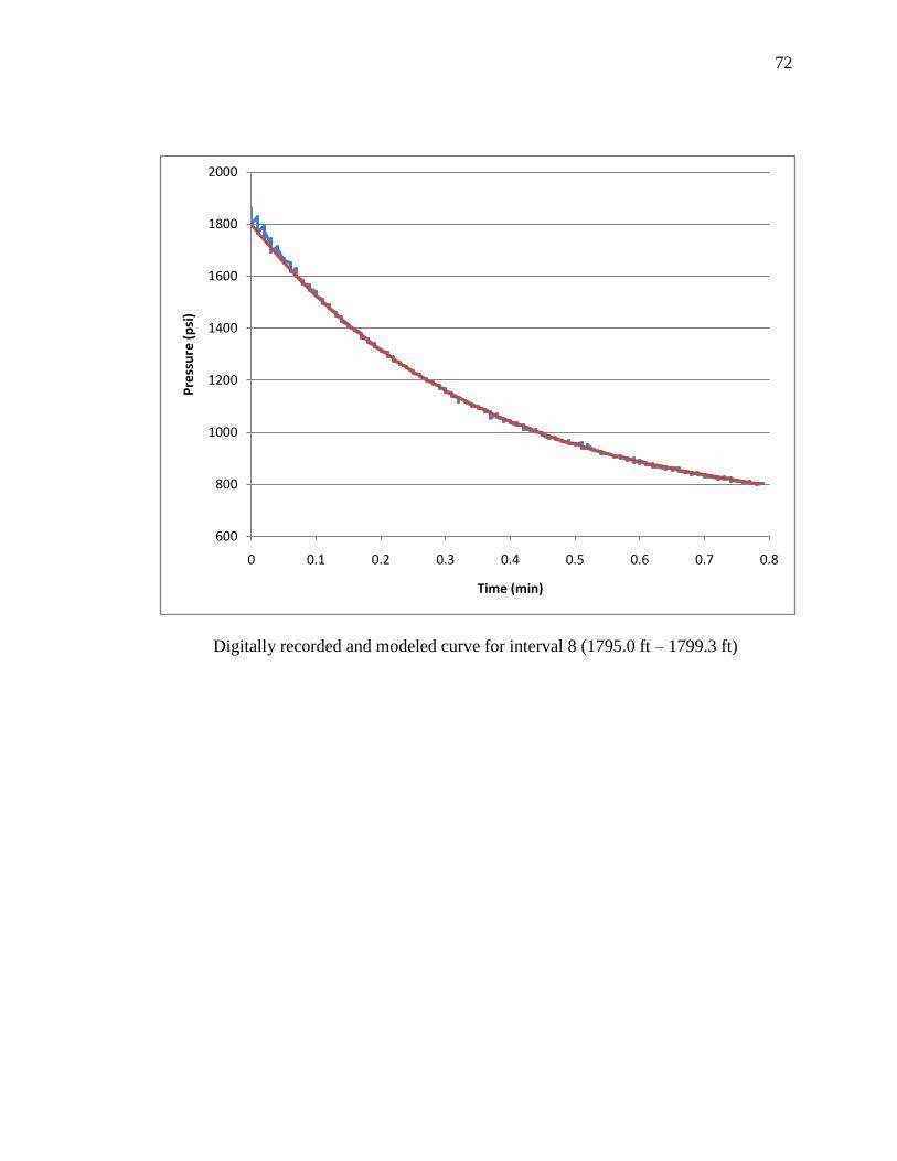
72

Digitally recorded and modeled curve for interval 8 (1795.0 ft – 1799.3 ft)

600

800

1000

1200

1400

1600

1800

2000

0 0.1 0.2 0.3 0.4 0.5 0.6 0.7 0.8

Pre

ssu

re (

psi

)

Time (min)

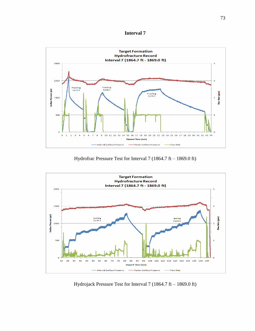
73

Interval 7

Hydrofrac Pressure Test for Interval 7 (1864.7 ft – 1869.0 ft)

Hydrojack Pressure Test for Interval 7 (1864.7 ft – 1869.0 ft)

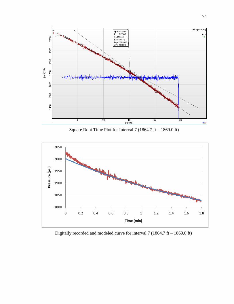
74

Square Root Time Plot for Interval 7 (1864.7 ft – 1869.0 ft)

Digitally recorded and modeled curve for interval 7 (1864.7 ft – 1869.0 ft)

1800

1850

1900

1950

2000

2050

0 0.2 0.4 0.6 0.8 1 1.2 1.4 1.6 1.8

Pre

ssu

re (

psi

)

Time (min)

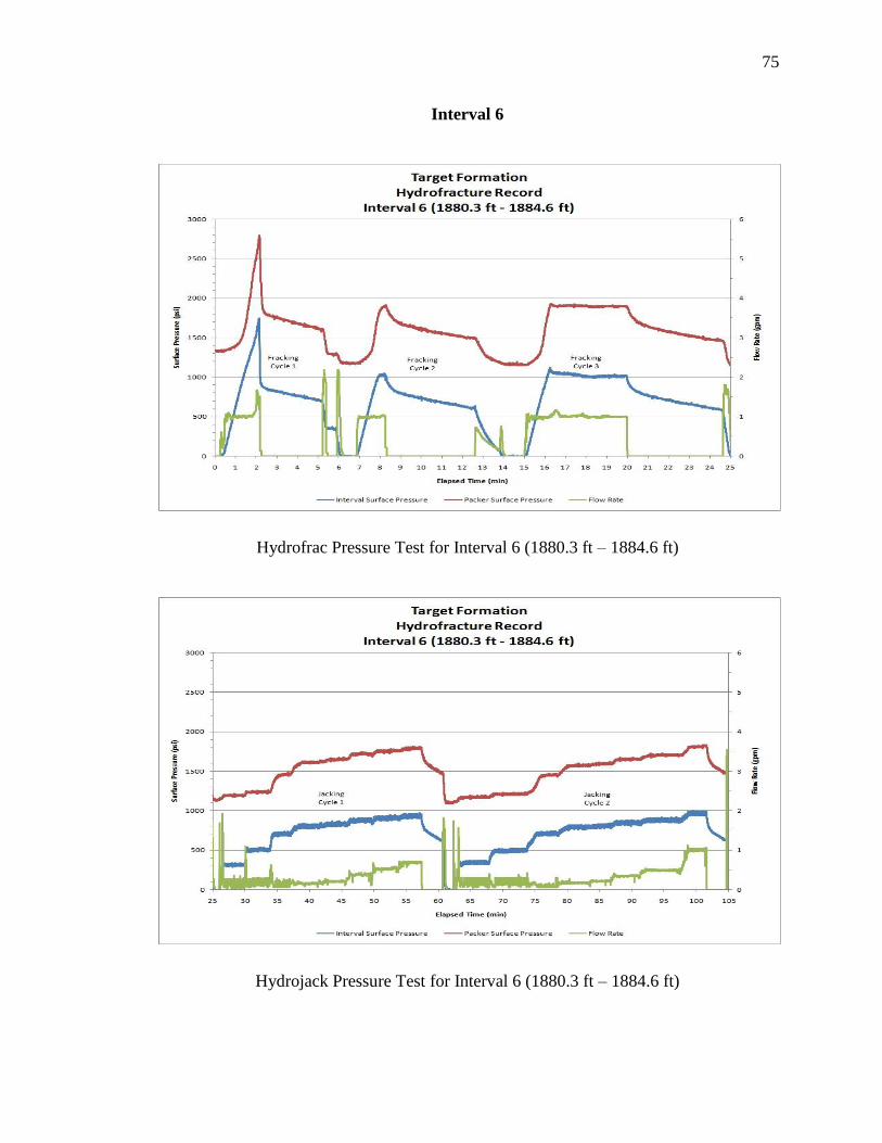
75

Interval 6

Hydrofrac Pressure Test for Interval 6 (1880.3 ft – 1884.6 ft)

Hydrojack Pressure Test for Interval 6 (1880.3 ft – 1884.6 ft)

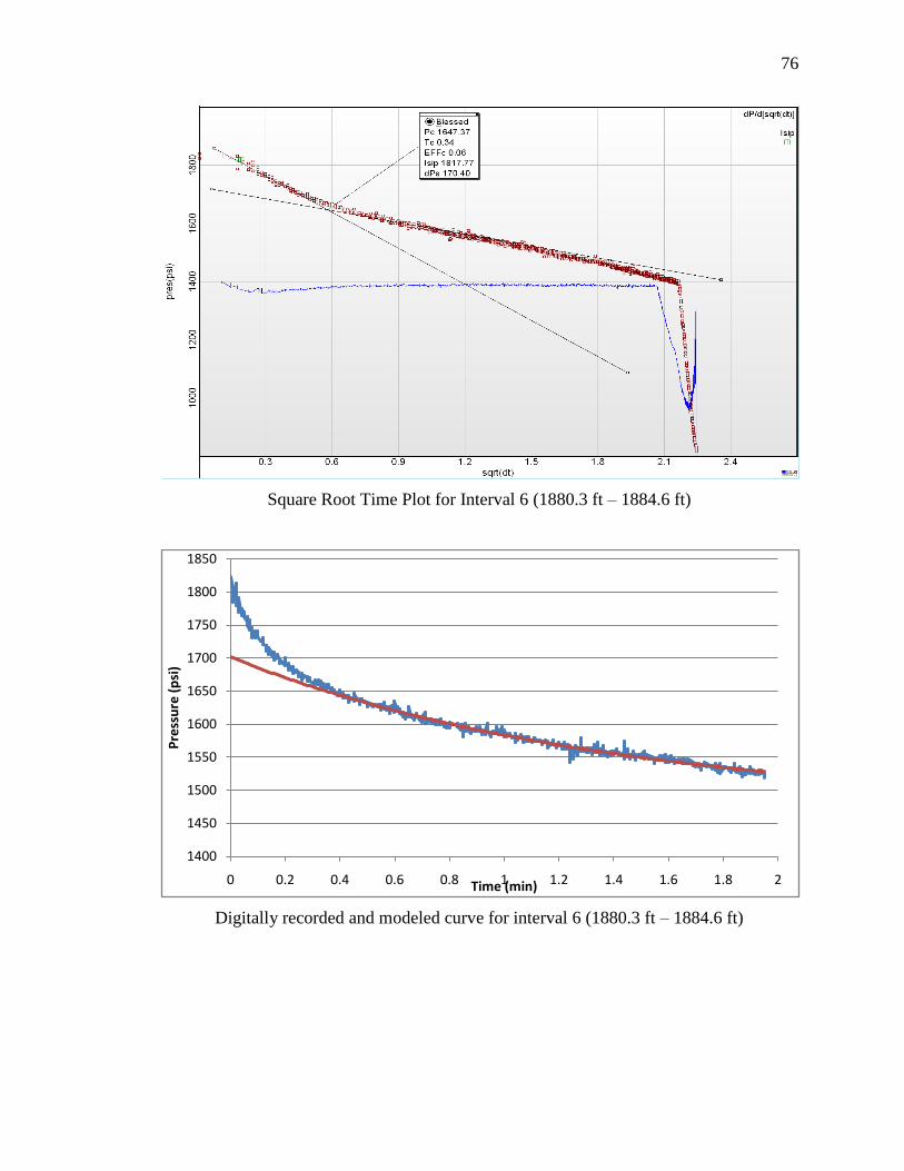
76

Square Root Time Plot for Interval 6 (1880.3 ft – 1884.6 ft)

Digitally recorded and modeled curve for interval 6 (1880.3 ft – 1884.6 ft)

1400

1450

1500

1550

1600

1650

1700

1750

1800

1850

0 0.2 0.4 0.6 0.8 1 1.2 1.4 1.6 1.8 2

Pre

ssu

re (

psi

)

Time (min)

77

Interval 5

Hydrofrac Pressure Test for Interval 5 (1942.3 ft – 1946.6 ft)

Hydrojack Pressure Test for Interval 5 (1942.3 ft – 1946.6 ft)

78

Square Root Time Plot for Interval 5 (1942.3 ft – 1946.6 ft)

Digitally recorded and modeled curve for interval 5

(1942.3 ft – 1946.6 ft)

1500

1550

1600

1650

1700

1750

1800

0 0.5 1 1.5 2 2.5

Pre

ssu

re (

psi

)

Time (min)

79

Interval 4

Hydrofrac Pressure Test for Interval 4 (1995.3 ft – 1996.3 ft)

Hydrojack Pressure Test for Interval 4 (1995.3 ft – 1996.3 ft)

80

Square Root Time Plot for Interval 4 (1995.3 ft – 1999.6 ft)

Digitally recorded and modeled curve for interval 4

(1995.3 ft – 1999.6 ft)

800

850

900

950

1000

1050

1100

1150

1200

1250

0 0.2 0.4 0.6 0.8 1 1.2 1.4 1.6 1.8

Pre

ssu

re (

psi

)

Time (min)

81

Interval 10

Hydrofrac Pressure Test for Interval 10 (2013.0 ft – 2017.3 ft)

Hydrojack Pressure Test for Interval 10 (2013.0 ft – 2017.3 ft)

82

Square Root Time Plot for Interval 10 (2013.0 ft – 2017.3 ft)

83

Interval 3

Hydrofrac Pressure Test for Interval 3 (2022.0 ft – 2026.3ft)

Hydrojack Pressure Test for Interval 3 (2022.0 ft – 2026.3ft)

84

Square Root Time Plot for Interval 3 (2022.0 ft – 2026.3 ft)

Digitally recorded and modeled curve for interval 3

(2022.0 ft – 2026.3 ft)

960

980

1000

1020

1040

1060

1080

1100

1120

1140

1160

1180

0 0.5 1 1.5 2 2.5

Pre

ssu

re (

psi

)

Time (min)

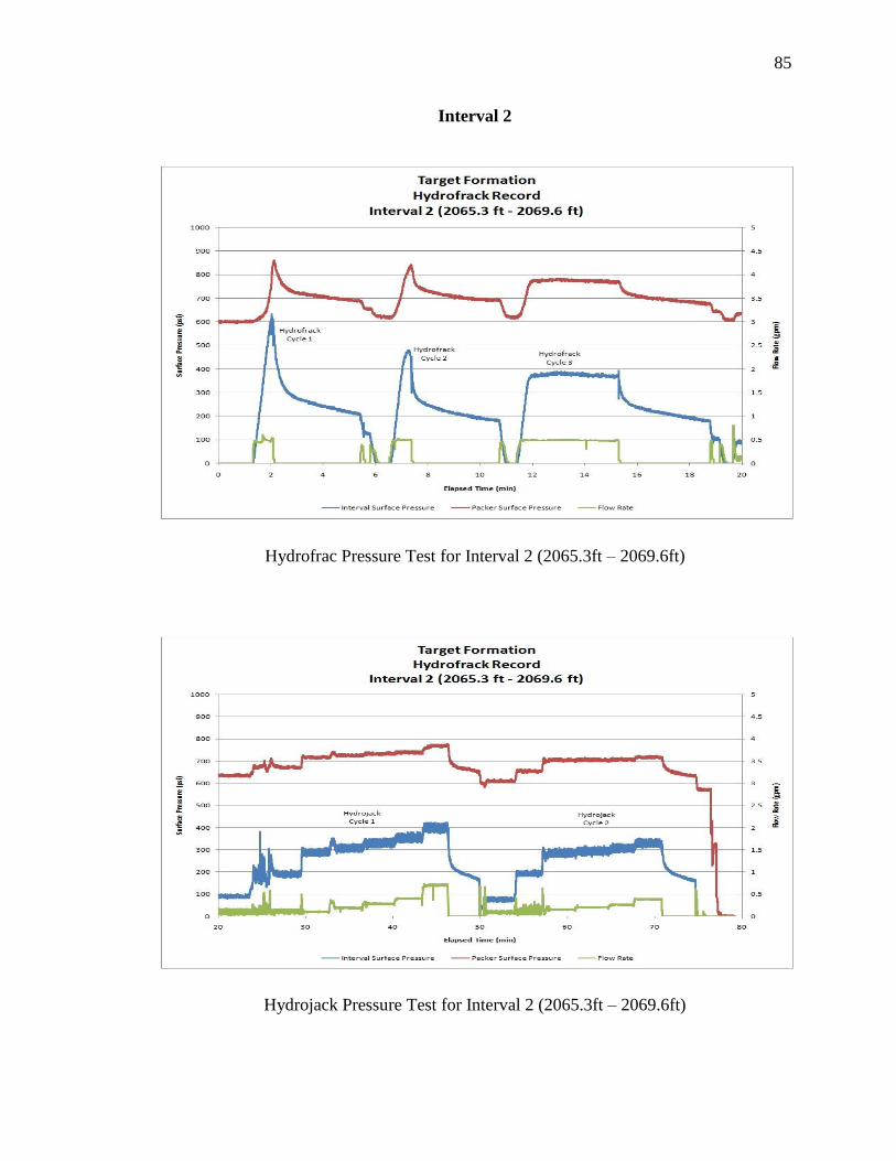
85

Interval 2

Hydrofrac Pressure Test for Interval 2 (2065.3ft – 2069.6ft)

Hydrojack Pressure Test for Interval 2 (2065.3ft – 2069.6ft)

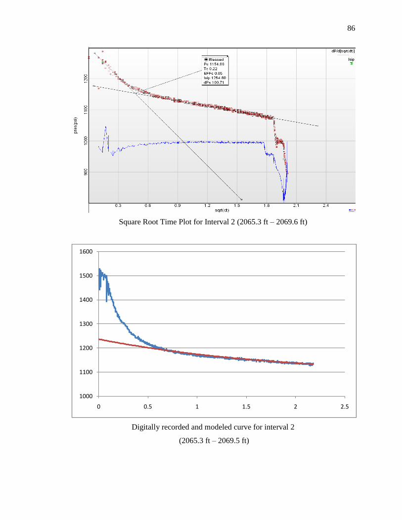
86

Square Root Time Plot for Interval 2 (2065.3 ft – 2069.6 ft)

Digitally recorded and modeled curve for interval 2

(2065.3 ft – 2069.5 ft)

1000

1100

1200

1300

1400

1500

1600

0 0.5 1 1.5 2 2.5

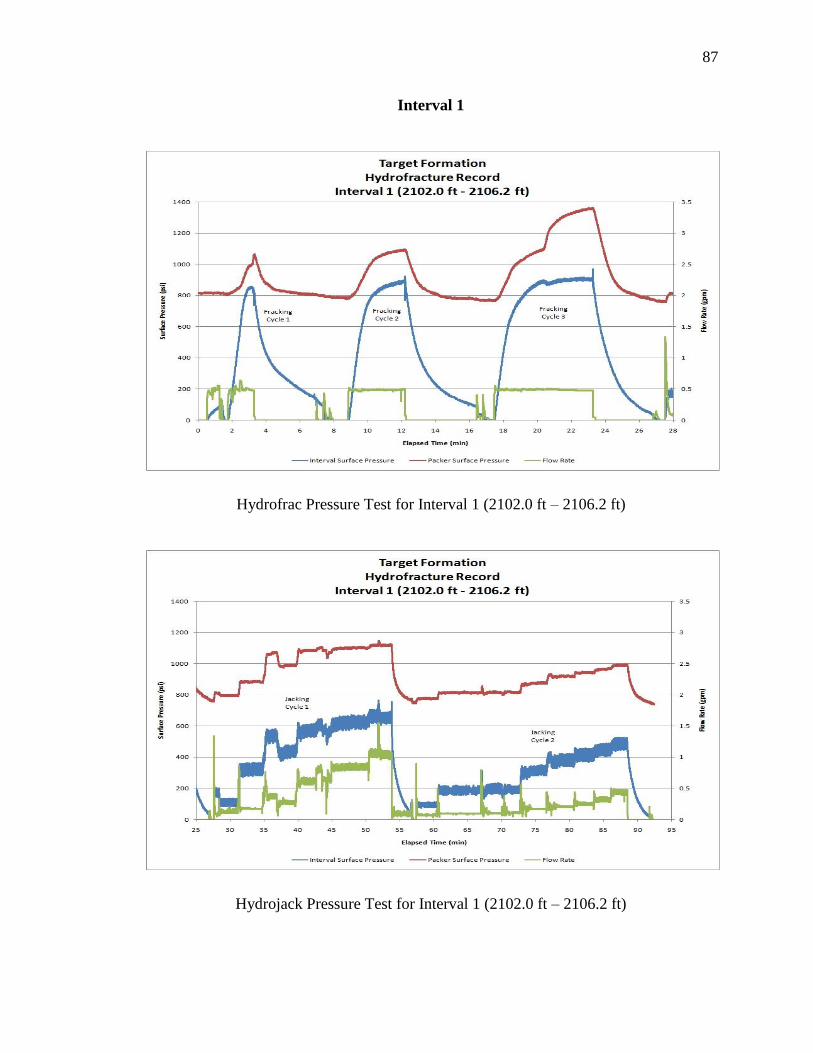
87

Interval 1

Hydrofrac Pressure Test for Interval 1 (2102.0 ft – 2106.2 ft)

Hydrojack Pressure Test for Interval 1 (2102.0 ft – 2106.2 ft)

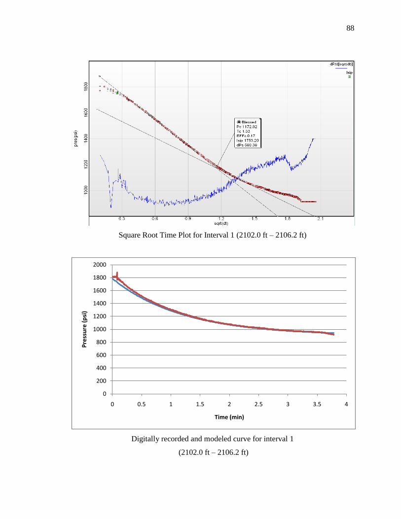
88

Square Root Time Plot for Interval 1 (2102.0 ft – 2106.2 ft)

Digitally recorded and modeled curve for interval 1

(2102.0 ft – 2106.2 ft)

0

200

400

600

800

1000

1200

1400

1600

1800

2000

0 0.5 1 1.5 2 2.5 3 3.5 4

Pre

ssu

re (

psi

)

Time (min)

89

APPENDIX B

OUTPUT TABLES FROM SAS

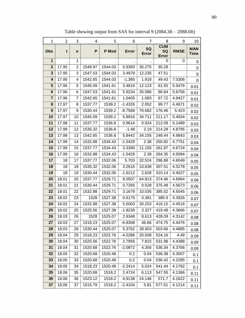
90

Table showing output from SAS for interval 9 (2084.3ft – 2088.6ft)

1 2 3 4 5 6 7 8 9 10

Obs t n P P Mod Error SQ

Error

CUM SQ

Error RMSE

MAN Time

1 . 1 . . . . 0 0 0 2 17.95 2 1549.97 1544.03 5.9393 35.275 35.28 . 0 3 17.95 3 1547.53 1544.03 3.4979 12.235 47.51 . 0 4 17.95 4 1542.65 1544.03 -1.385 1.918 49.43 7.0306 0 5 17.96 5 1545.09 1541.61 3.4819 12.123 61.55 5.5476 0.01 6 17.96 6 1547.53 1541.61 5.9234 35.086 96.64 5.6756 0.01 7 17.96 7 1542.65 1541.61 1.0405 1.083 97.72 4.9427 0.01 8 17.97 8 1537.77 1539.2 -1.4326 2.052 99.77 4.4671 0.02 9 17.97 9 1530.44 1539.2 -8.7568 76.682 176.46 5.423 0.02

10 17.97 10 1545.09 1539.2 5.8916 34.711 211.17 5.4924 0.02 11 17.98 11 1537.77 1536.8 0.9614 0.924 212.09 5.1489 0.03 12 17.98 12 1535.32 1536.8 -1.48 2.19 214.28 4.8795 0.03 13 17.98 13 1542.65 1536.8 5.8442 34.155 248.44 4.9843 0.03 14 17.99 14 1532.88 1534.43 -1.5429 2.38 250.82 4.7751 0.04 15 17.99 15 1537.77 1534.43 3.3399 11.155 261.97 4.6724 0.04 16 17.99 16 1532.88 1534.43 -1.5429 2.38 264.35 4.5094 0.04 17 18 17 1537.77 1532.06 5.703 32.524 296.88 4.6049 0.05 18 18 18 1535.32 1532.06 3.2616 10.638 307.51 4.5278 0.05 19 18 19 1530.44 1532.06 -1.6212 2.628 310.14 4.4027 0.05 20 18.01 20 1537.77 1529.71 8.0507 64.813 374.96 4.6964 0.06 21 18.01 21 1530.44 1529.71 0.7265 0.528 375.48 4.5673 0.06 22 18.01 22 1532.88 1529.71 3.1679 10.035 385.52 4.5045 0.06 23 18.02 23 1528 1527.38 0.6175 0.381 385.9 4.3926 0.07 24 18.02 24 1532.88 1527.38 5.5003 30.253 416.15 4.4516 0.07 25 18.02 25 1525.56 1527.38 -1.8239 3.327 419.48 4.3666 0.07 26 18.03 26 1528 1525.07 2.9348 8.613 428.09 4.3142 0.08 27 18.03 27 1518.23 1525.07 -6.8308 46.66 474.75 4.4476 0.08 28 18.03 28 1530.44 1525.07 5.3762 28.903 503.66 4.4885 0.08 29 18.04 29 1518.23 1522.76 -4.5286 20.508 524.16 4.49 0.09 30 18.04 30 1525.56 1522.76 2.7956 7.815 531.98 4.4388 0.09 31 18.04 31 1520.68 1522.76 -2.0872 4.356 536.34 4.3766 0.09 32 18.05 32 1520.68 1520.48 0.2 0.04 536.38 4.3007 0.1 33 18.05 33 1520.68 1520.48 0.2 0.04 536.42 4.2285 0.1 34 18.05 34 1518.23 1520.48 -2.2414 5.024 541.44 4.1792 0.1 35 18.06 35 1520.68 1518.2 2.4724 6.113 547.55 4.1366 0.11 36 18.06 36 1523.12 1518.2 4.9138 24.146 571.7 4.1622 0.11 37 18.06 37 1515.79 1518.2 -2.4104 5.81 577.51 4.1214 0.11

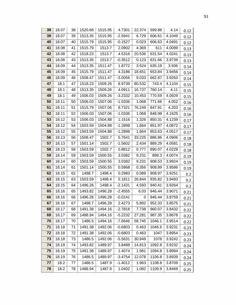
91

38 18.07 38 1520.68 1515.95 4.7301 22.374 599.88 4.14 0.12 39 18.07 39 1513.35 1515.95 -2.5941 6.729 606.61 4.1049 0.12 40 18.07 40 1515.79 1515.95 -0.1527 0.023 606.63 4.0491 0.12 41 18.08 41 1515.79 1513.7 2.0902 4.369 611 4.0099 0.13 42 18.08 42 1518.23 1513.7 4.5316 20.536 631.54 4.0241 0.13 43 18.08 43 1513.35 1513.7 -0.3512 0.123 631.66 3.9739 0.13 44 18.09 44 1513.35 1511.47 1.8772 3.524 635.19 3.936 0.14 45 18.09 45 1515.79 1511.47 4.3186 18.651 653.84 3.9456 0.14 46 18.09 46 1508.47 1511.47 -3.0056 9.033 662.87 3.9263 0.14 47 18.1 47 1518.23 1509.26 8.9739 80.532 743.4 4.1104 0.15 48 18.1 48 1513.35 1509.26 4.0911 16.737 760.14 4.11 0.15 49 18.1 49 1506.03 1509.26 -3.2332 10.453 770.59 4.0929 0.15 50 18.11 50 1506.03 1507.06 -1.0336 1.068 771.66 4.052 0.16 51 18.11 51 1515.79 1507.06 8.7321 76.249 847.91 4.203 0.16 52 18.11 52 1506.03 1507.06 -1.0336 1.068 848.98 4.1625 0.16 53 18.12 53 1506.03 1504.88 1.1516 1.326 850.31 4.1239 0.17 54 18.12 54 1503.59 1504.88 -1.2898 1.664 851.97 4.0872 0.17 55 18.12 55 1503.59 1504.88 -1.2898 1.664 853.63 4.0517 0.17 56 18.13 56 1508.47 1502.7 5.7641 33.225 886.86 4.0906 0.18 57 18.13 57 1501.14 1502.7 -1.5602 2.434 889.29 4.0581 0.18 58 18.13 58 1503.59 1502.7 0.8812 0.777 890.07 4.0228 0.18 59 18.14 59 1503.59 1500.55 3.0382 9.231 899.3 4.0074 0.19 60 18.14 60 1503.59 1500.55 3.0382 9.231 908.53 3.9924 0.19 61 18.14 61 1501.14 1500.55 0.5968 0.356 908.89 3.9586 0.19 62 18.15 62 1498.7 1498.4 0.2983 0.089 908.97 3.9251 0.2 63 18.15 63 1503.59 1498.4 5.1811 26.844 935.82 3.9493 0.2 64 18.15 64 1496.26 1498.4 -2.1431 4.593 940.41 3.9264 0.2 65 18.16 65 1493.82 1496.28 -2.4555 6.03 946.44 3.9071 0.21 66 18.16 66 1496.26 1496.28 -0.0141 0 946.44 3.8759 0.21 67 18.16 67 1498.7 1496.28 2.4273 5.892 952.33 3.8575 0.21 68 18.17 68 1491.38 1494.16 -2.7818 7.738 960.07 3.8432 0.22 69 18.17 69 1488.94 1494.16 -5.2232 27.281 987.35 3.8678 0.22 70 18.17 70 1486.5 1494.16 -7.6646 58.745 1046.1 3.9514 0.22 71 18.18 71 1491.38 1492.06 -0.6803 0.463 1046.6 3.9231 0.23 72 18.18 72 1491.38 1492.06 -0.6803 0.463 1047 3.8954 0.23 73 18.18 73 1486.5 1492.06 -5.5631 30.949 1078 3.9242 0.23 74 18.19 74 1493.82 1489.97 3.8488 14.813 1092.8 3.9232 0.24 75 18.19 75 1491.38 1489.97 1.4074 1.981 1094.8 3.8994 0.24 76 18.19 76 1486.5 1489.97 -3.4754 12.078 1106.8 3.8939 0.24 77 18.2 77 1486.5 1487.9 -1.4012 1.963 1108.8 3.8709 0.25 78 18.2 78 1488.94 1487.9 1.0402 1.082 1109.9 3.8469 0.25

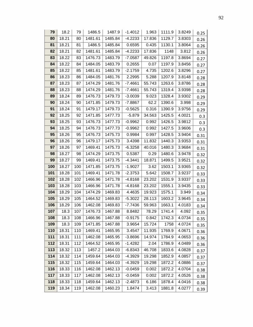
92

79 18.2 79 1486.5 1487.9 -1.4012 1.963 1111.9 3.8249 0.25 80 18.21 80 1481.61 1485.84 -4.2233 17.836 1129.7 3.8303 0.26 81 18.21 81 1486.5 1485.84 0.6595 0.435 1130.1 3.8064 0.26 82 18.21 82 1481.61 1485.84 -4.2233 17.836 1148 3.812 0.26 83 18.22 83 1476.73 1483.79 -7.0587 49.826 1197.8 3.8694 0.27 84 18.22 84 1484.05 1483.79 0.2655 0.07 1197.9 3.8456 0.27 85 18.22 85 1481.61 1483.79 -2.1759 4.735 1202.6 3.8296 0.27 86 18.23 86 1484.05 1481.76 2.2995 5.288 1207.9 3.8148 0.28 87 18.23 87 1474.29 1481.76 -7.4661 55.743 1263.6 3.8786 0.28 88 18.23 88 1474.29 1481.76 -7.4661 55.743 1319.4 3.9398 0.28 89 18.24 89 1476.73 1479.73 -3.0039 9.023 1328.4 3.9302 0.29 90 18.24 90 1471.85 1479.73 -7.8867 62.2 1390.6 3.998 0.29 91 18.24 91 1479.17 1479.73 -0.5625 0.316 1390.9 3.9756 0.29 92 18.25 92 1471.85 1477.73 -5.879 34.563 1425.5 4.0021 0.3 93 18.25 93 1476.73 1477.73 -0.9962 0.992 1426.5 3.9812 0.3 94 18.25 94 1476.73 1477.73 -0.9962 0.992 1427.5 3.9606 0.3 95 18.26 95 1476.73 1475.73 0.9984 0.997 1428.5 3.9404 0.31 96 18.26 96 1479.17 1475.73 3.4398 11.832 1440.3 3.9353 0.31 97 18.26 97 1469.41 1475.73 -6.3258 40.016 1480.3 3.9684 0.31 98 18.27 98 1474.29 1473.75 0.5387 0.29 1480.6 3.9478 0.32 99 18.27 99 1469.41 1473.75 -4.3441 18.871 1499.5 3.9521 0.32

100 18.27 100 1471.85 1473.75 -1.9027 3.62 1503.1 3.9365 0.32 101 18.28 101 1469.41 1471.78 -2.3753 5.642 1508.7 3.9237 0.33 102 18.28 102 1466.96 1471.78 -4.8168 23.202 1531.9 3.9337 0.33 103 18.28 103 1466.96 1471.78 -4.8168 23.202 1555.1 3.9435 0.33 104 18.29 104 1474.29 1469.83 4.4635 19.923 1575.1 3.949 0.34 105 18.29 105 1464.52 1469.83 -5.3022 28.113 1603.2 3.9645 0.34 106 18.29 106 1462.08 1469.83 -7.7436 59.963 1663.1 4.0183 0.34 107 18.3 107 1476.73 1467.88 8.8482 78.29 1741.4 4.092 0.35 108 18.3 108 1466.96 1467.88 -0.9175 0.842 1742.3 4.0734 0.35 109 18.3 109 1471.85 1467.88 3.9654 15.724 1758 4.0724 0.35 110 18.31 110 1469.41 1465.95 3.4547 11.935 1769.9 4.0671 0.36 111 18.31 111 1462.08 1465.95 -3.8696 14.974 1784.9 4.0653 0.36 112 18.31 112 1464.52 1465.95 -1.4282 2.04 1786.9 4.0489 0.36 113 18.32 113 1457.2 1464.03 -6.8343 46.708 1833.6 4.0828 0.37 114 18.32 114 1459.64 1464.03 -4.3929 19.298 1852.9 4.0857 0.37 115 18.32 115 1459.64 1464.03 -4.3929 19.298 1872.2 4.0886 0.37 116 18.33 116 1462.08 1462.13 -0.0459 0.002 1872.2 4.0704 0.38 117 18.33 117 1462.08 1462.13 -0.0459 0.002 1872.2 4.0526 0.38 118 18.33 118 1459.64 1462.13 -2.4873 6.186 1878.4 4.0416 0.38 119 18.34 119 1462.08 1460.23 1.8474 3.413 1881.8 4.0277 0.39

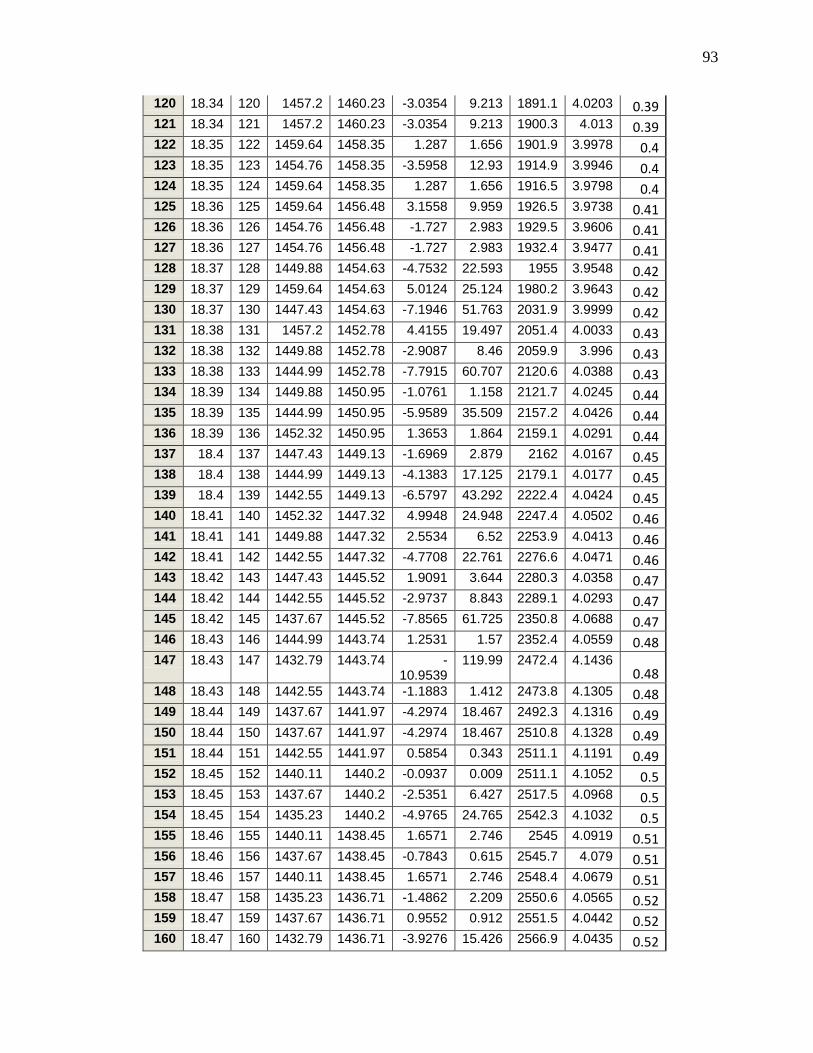
93

120 18.34 120 1457.2 1460.23 -3.0354 9.213 1891.1 4.0203 0.39 121 18.34 121 1457.2 1460.23 -3.0354 9.213 1900.3 4.013 0.39 122 18.35 122 1459.64 1458.35 1.287 1.656 1901.9 3.9978 0.4 123 18.35 123 1454.76 1458.35 -3.5958 12.93 1914.9 3.9946 0.4 124 18.35 124 1459.64 1458.35 1.287 1.656 1916.5 3.9798 0.4 125 18.36 125 1459.64 1456.48 3.1558 9.959 1926.5 3.9738 0.41 126 18.36 126 1454.76 1456.48 -1.727 2.983 1929.5 3.9606 0.41 127 18.36 127 1454.76 1456.48 -1.727 2.983 1932.4 3.9477 0.41 128 18.37 128 1449.88 1454.63 -4.7532 22.593 1955 3.9548 0.42 129 18.37 129 1459.64 1454.63 5.0124 25.124 1980.2 3.9643 0.42 130 18.37 130 1447.43 1454.63 -7.1946 51.763 2031.9 3.9999 0.42 131 18.38 131 1457.2 1452.78 4.4155 19.497 2051.4 4.0033 0.43 132 18.38 132 1449.88 1452.78 -2.9087 8.46 2059.9 3.996 0.43 133 18.38 133 1444.99 1452.78 -7.7915 60.707 2120.6 4.0388 0.43 134 18.39 134 1449.88 1450.95 -1.0761 1.158 2121.7 4.0245 0.44 135 18.39 135 1444.99 1450.95 -5.9589 35.509 2157.2 4.0426 0.44 136 18.39 136 1452.32 1450.95 1.3653 1.864 2159.1 4.0291 0.44 137 18.4 137 1447.43 1449.13 -1.6969 2.879 2162 4.0167 0.45 138 18.4 138 1444.99 1449.13 -4.1383 17.125 2179.1 4.0177 0.45 139 18.4 139 1442.55 1449.13 -6.5797 43.292 2222.4 4.0424 0.45 140 18.41 140 1452.32 1447.32 4.9948 24.948 2247.4 4.0502 0.46 141 18.41 141 1449.88 1447.32 2.5534 6.52 2253.9 4.0413 0.46 142 18.41 142 1442.55 1447.32 -4.7708 22.761 2276.6 4.0471 0.46 143 18.42 143 1447.43 1445.52 1.9091 3.644 2280.3 4.0358 0.47 144 18.42 144 1442.55 1445.52 -2.9737 8.843 2289.1 4.0293 0.47 145 18.42 145 1437.67 1445.52 -7.8565 61.725 2350.8 4.0688 0.47 146 18.43 146 1444.99 1443.74 1.2531 1.57 2352.4 4.0559 0.48 147 18.43 147 1432.79 1443.74 -

10.9539 119.99 2472.4 4.1436

0.48 148 18.43 148 1442.55 1443.74 -1.1883 1.412 2473.8 4.1305 0.48 149 18.44 149 1437.67 1441.97 -4.2974 18.467 2492.3 4.1316 0.49 150 18.44 150 1437.67 1441.97 -4.2974 18.467 2510.8 4.1328 0.49 151 18.44 151 1442.55 1441.97 0.5854 0.343 2511.1 4.1191 0.49 152 18.45 152 1440.11 1440.2 -0.0937 0.009 2511.1 4.1052 0.5 153 18.45 153 1437.67 1440.2 -2.5351 6.427 2517.5 4.0968 0.5 154 18.45 154 1435.23 1440.2 -4.9765 24.765 2542.3 4.1032 0.5 155 18.46 155 1440.11 1438.45 1.6571 2.746 2545 4.0919 0.51 156 18.46 156 1437.67 1438.45 -0.7843 0.615 2545.7 4.079 0.51 157 18.46 157 1440.11 1438.45 1.6571 2.746 2548.4 4.0679 0.51 158 18.47 158 1435.23 1436.71 -1.4862 2.209 2550.6 4.0565 0.52 159 18.47 159 1437.67 1436.71 0.9552 0.912 2551.5 4.0442 0.52 160 18.47 160 1432.79 1436.71 -3.9276 15.426 2566.9 4.0435 0.52

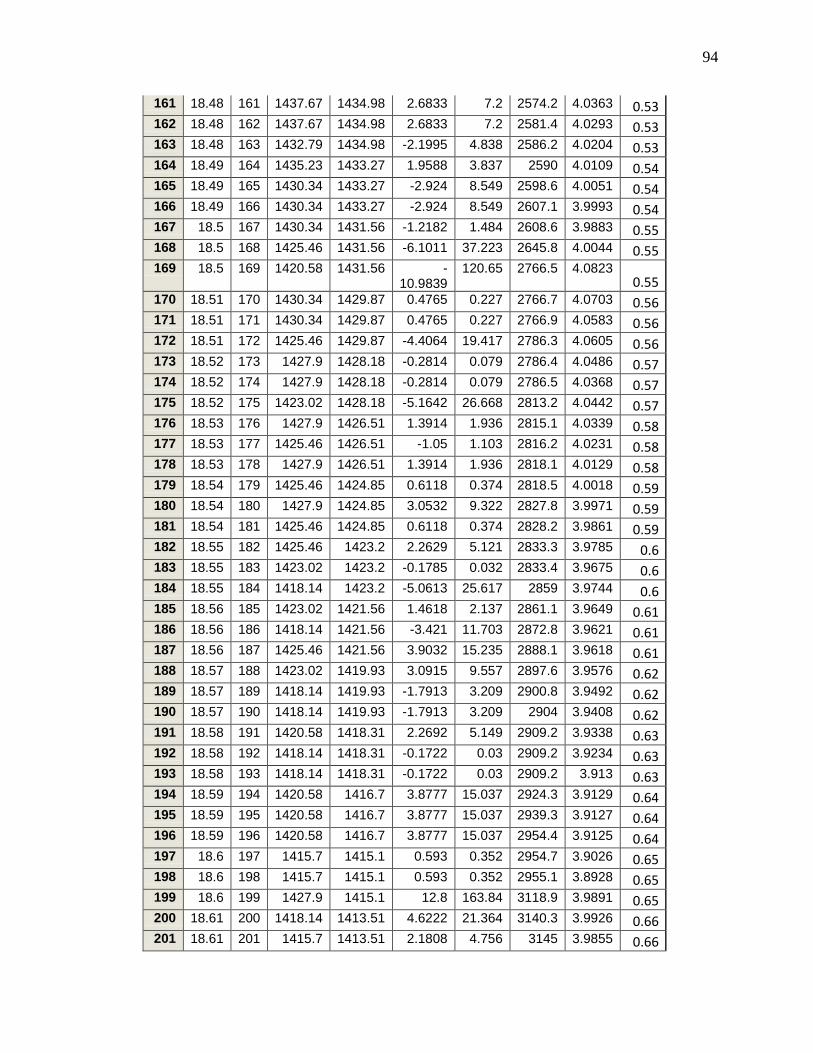
94

161 18.48 161 1437.67 1434.98 2.6833 7.2 2574.2 4.0363 0.53 162 18.48 162 1437.67 1434.98 2.6833 7.2 2581.4 4.0293 0.53 163 18.48 163 1432.79 1434.98 -2.1995 4.838 2586.2 4.0204 0.53 164 18.49 164 1435.23 1433.27 1.9588 3.837 2590 4.0109 0.54 165 18.49 165 1430.34 1433.27 -2.924 8.549 2598.6 4.0051 0.54 166 18.49 166 1430.34 1433.27 -2.924 8.549 2607.1 3.9993 0.54 167 18.5 167 1430.34 1431.56 -1.2182 1.484 2608.6 3.9883 0.55 168 18.5 168 1425.46 1431.56 -6.1011 37.223 2645.8 4.0044 0.55 169 18.5 169 1420.58 1431.56 -

10.9839 120.65 2766.5 4.0823

0.55 170 18.51 170 1430.34 1429.87 0.4765 0.227 2766.7 4.0703 0.56 171 18.51 171 1430.34 1429.87 0.4765 0.227 2766.9 4.0583 0.56 172 18.51 172 1425.46 1429.87 -4.4064 19.417 2786.3 4.0605 0.56 173 18.52 173 1427.9 1428.18 -0.2814 0.079 2786.4 4.0486 0.57 174 18.52 174 1427.9 1428.18 -0.2814 0.079 2786.5 4.0368 0.57 175 18.52 175 1423.02 1428.18 -5.1642 26.668 2813.2 4.0442 0.57 176 18.53 176 1427.9 1426.51 1.3914 1.936 2815.1 4.0339 0.58 177 18.53 177 1425.46 1426.51 -1.05 1.103 2816.2 4.0231 0.58 178 18.53 178 1427.9 1426.51 1.3914 1.936 2818.1 4.0129 0.58 179 18.54 179 1425.46 1424.85 0.6118 0.374 2818.5 4.0018 0.59 180 18.54 180 1427.9 1424.85 3.0532 9.322 2827.8 3.9971 0.59 181 18.54 181 1425.46 1424.85 0.6118 0.374 2828.2 3.9861 0.59 182 18.55 182 1425.46 1423.2 2.2629 5.121 2833.3 3.9785 0.6 183 18.55 183 1423.02 1423.2 -0.1785 0.032 2833.4 3.9675 0.6 184 18.55 184 1418.14 1423.2 -5.0613 25.617 2859 3.9744 0.6 185 18.56 185 1423.02 1421.56 1.4618 2.137 2861.1 3.9649 0.61 186 18.56 186 1418.14 1421.56 -3.421 11.703 2872.8 3.9621 0.61 187 18.56 187 1425.46 1421.56 3.9032 15.235 2888.1 3.9618 0.61 188 18.57 188 1423.02 1419.93 3.0915 9.557 2897.6 3.9576 0.62 189 18.57 189 1418.14 1419.93 -1.7913 3.209 2900.8 3.9492 0.62 190 18.57 190 1418.14 1419.93 -1.7913 3.209 2904 3.9408 0.62 191 18.58 191 1420.58 1418.31 2.2692 5.149 2909.2 3.9338 0.63 192 18.58 192 1418.14 1418.31 -0.1722 0.03 2909.2 3.9234 0.63 193 18.58 193 1418.14 1418.31 -0.1722 0.03 2909.2 3.913 0.63 194 18.59 194 1420.58 1416.7 3.8777 15.037 2924.3 3.9129 0.64 195 18.59 195 1420.58 1416.7 3.8777 15.037 2939.3 3.9127 0.64 196 18.59 196 1420.58 1416.7 3.8777 15.037 2954.4 3.9125 0.64 197 18.6 197 1415.7 1415.1 0.593 0.352 2954.7 3.9026 0.65 198 18.6 198 1415.7 1415.1 0.593 0.352 2955.1 3.8928 0.65 199 18.6 199 1427.9 1415.1 12.8 163.84 3118.9 3.9891 0.65 200 18.61 200 1418.14 1413.51 4.6222 21.364 3140.3 3.9926 0.66 201 18.61 201 1415.7 1413.51 2.1808 4.756 3145 3.9855 0.66

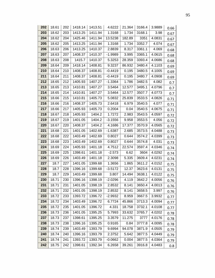
95

202 18.61 202 1418.14 1413.51 4.6222 21.364 3166.4 3.9889 0.66 203 18.62 203 1413.25 1411.94 1.3168 1.734 3168.1 3.98 0.67 204 18.62 204 1425.46 1411.94 13.5238 182.89 3351 4.0831 0.67 205 18.62 205 1413.25 1411.94 1.3168 1.734 3352.7 4.074 0.67 206 18.63 206 1413.25 1410.37 2.8839 8.317 3361.1 4.069 0.68 207 18.63 207 1408.37 1410.37 -1.9989 3.995 3365.1 4.0615 0.68 208 18.63 208 1415.7 1410.37 5.3253 28.359 3393.4 4.0686 0.68 209 18.64 209 1418.14 1408.81 9.3237 86.932 3480.4 4.1103 0.69 210 18.64 210 1408.37 1408.81 -0.4419 0.195 3480.5 4.1005 0.69 211 18.64 211 1408.37 1408.81 -0.4419 0.195 3480.7 4.0908 0.69 212 18.65 212 1405.93 1407.27 -1.3364 1.786 3482.5 4.082 0.7 213 18.65 213 1410.81 1407.27 3.5464 12.577 3495.1 4.0796 0.7 214 18.65 214 1410.81 1407.27 3.5464 12.577 3507.7 4.0773 0.7 215 18.66 215 1410.81 1405.73 5.0832 25.839 3533.5 4.0826 0.71 216 18.66 216 1408.37 1405.73 2.6418 6.979 3540.5 4.077 0.71 217 18.66 217 1405.93 1405.73 0.2004 0.04 3540.5 4.0675 0.71 218 18.67 218 1405.93 1404.2 1.7272 2.983 3543.5 4.0597 0.72 219 18.67 219 1401.05 1404.2 -3.1556 9.958 3553.5 4.056 0.72 220 18.67 220 1408.37 1404.2 4.1686 17.377 3570.9 4.0565 0.72 221 18.68 221 1401.05 1402.69 -1.6387 2.685 3573.5 4.0488 0.73 222 18.68 222 1403.49 1402.69 0.8027 0.644 3574.2 4.0399 0.73 223 18.68 223 1403.49 1402.69 0.8027 0.644 3574.8 4.031 0.73 224 18.69 224 1405.93 1401.18 4.7512 22.574 3597.4 4.0346 0.74 225 18.69 225 1398.61 1401.18 -2.573 6.62 3604 4.0292 0.74 226 18.69 226 1403.49 1401.18 2.3098 5.335 3609.4 4.0231 0.74 227 18.7 227 1401.05 1399.68 1.3656 1.865 3611.2 4.0152 0.75 228 18.7 228 1396.16 1399.68 -3.5172 12.37 3623.6 4.0131 0.75 229 18.7 229 1403.49 1399.68 3.807 14.494 3638.1 4.0122 0.75 230 18.71 230 1396.16 1398.19 -2.0296 4.119 3642.2 4.0056 0.76 231 18.71 231 1401.05 1398.19 2.8532 8.141 3650.4 4.0013 0.76 232 18.71 232 1401.05 1398.19 2.8532 8.141 3658.5 3.997 0.76 233 18.72 233 1393.72 1396.72 -2.9932 8.959 3667.5 3.9932 0.77 234 18.72 234 1403.49 1396.72 6.7724 45.866 3713.3 4.0094 0.77 235 18.72 235 1401.05 1396.72 4.331 18.758 3732.1 4.0108 0.77 236 18.73 236 1401.05 1395.25 5.7993 33.632 3765.7 4.0202 0.78 237 18.73 237 1398.61 1395.25 3.3579 11.275 3777 4.0176 0.78 238 18.73 238 1396.16 1395.25 0.9165 0.84 3777.8 4.0095 0.78 239 18.74 239 1403.49 1393.79 9.6994 94.078 3871.9 4.0505 0.79 240 18.74 240 1396.16 1393.79 2.3752 5.642 3877.5 4.0449 0.79 241 18.74 241 1393.72 1393.79 -0.0662 0.004 3877.5 4.0364 0.79 242 18.75 242 1398.61 1392.34 6.2658 39.261 3916.8 4.0483 0.8

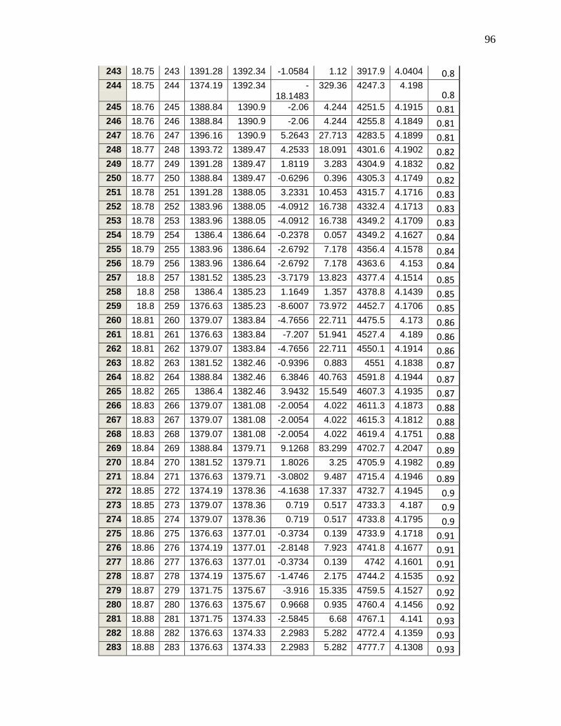
96

243 18.75 243 1391.28 1392.34 -1.0584 1.12 3917.9 4.0404 0.8 244 18.75 244 1374.19 1392.34 -

18.1483 329.36 4247.3 4.198

0.8 245 18.76 245 1388.84 1390.9 -2.06 4.244 4251.5 4.1915 0.81 246 18.76 246 1388.84 1390.9 -2.06 4.244 4255.8 4.1849 0.81 247 18.76 247 1396.16 1390.9 5.2643 27.713 4283.5 4.1899 0.81 248 18.77 248 1393.72 1389.47 4.2533 18.091 4301.6 4.1902 0.82 249 18.77 249 1391.28 1389.47 1.8119 3.283 4304.9 4.1832 0.82 250 18.77 250 1388.84 1389.47 -0.6296 0.396 4305.3 4.1749 0.82 251 18.78 251 1391.28 1388.05 3.2331 10.453 4315.7 4.1716 0.83 252 18.78 252 1383.96 1388.05 -4.0912 16.738 4332.4 4.1713 0.83 253 18.78 253 1383.96 1388.05 -4.0912 16.738 4349.2 4.1709 0.83 254 18.79 254 1386.4 1386.64 -0.2378 0.057 4349.2 4.1627 0.84 255 18.79 255 1383.96 1386.64 -2.6792 7.178 4356.4 4.1578 0.84 256 18.79 256 1383.96 1386.64 -2.6792 7.178 4363.6 4.153 0.84 257 18.8 257 1381.52 1385.23 -3.7179 13.823 4377.4 4.1514 0.85 258 18.8 258 1386.4 1385.23 1.1649 1.357 4378.8 4.1439 0.85 259 18.8 259 1376.63 1385.23 -8.6007 73.972 4452.7 4.1706 0.85 260 18.81 260 1379.07 1383.84 -4.7656 22.711 4475.5 4.173 0.86 261 18.81 261 1376.63 1383.84 -7.207 51.941 4527.4 4.189 0.86 262 18.81 262 1379.07 1383.84 -4.7656 22.711 4550.1 4.1914 0.86 263 18.82 263 1381.52 1382.46 -0.9396 0.883 4551 4.1838 0.87 264 18.82 264 1388.84 1382.46 6.3846 40.763 4591.8 4.1944 0.87 265 18.82 265 1386.4 1382.46 3.9432 15.549 4607.3 4.1935 0.87 266 18.83 266 1379.07 1381.08 -2.0054 4.022 4611.3 4.1873 0.88 267 18.83 267 1379.07 1381.08 -2.0054 4.022 4615.3 4.1812 0.88 268 18.83 268 1379.07 1381.08 -2.0054 4.022 4619.4 4.1751 0.88 269 18.84 269 1388.84 1379.71 9.1268 83.299 4702.7 4.2047 0.89 270 18.84 270 1381.52 1379.71 1.8026 3.25 4705.9 4.1982 0.89 271 18.84 271 1376.63 1379.71 -3.0802 9.487 4715.4 4.1946 0.89 272 18.85 272 1374.19 1378.36 -4.1638 17.337 4732.7 4.1945 0.9 273 18.85 273 1379.07 1378.36 0.719 0.517 4733.3 4.187 0.9 274 18.85 274 1379.07 1378.36 0.719 0.517 4733.8 4.1795 0.9 275 18.86 275 1376.63 1377.01 -0.3734 0.139 4733.9 4.1718 0.91 276 18.86 276 1374.19 1377.01 -2.8148 7.923 4741.8 4.1677 0.91 277 18.86 277 1376.63 1377.01 -0.3734 0.139 4742 4.1601 0.91 278 18.87 278 1374.19 1375.67 -1.4746 2.175 4744.2 4.1535 0.92 279 18.87 279 1371.75 1375.67 -3.916 15.335 4759.5 4.1527 0.92 280 18.87 280 1376.63 1375.67 0.9668 0.935 4760.4 4.1456 0.92 281 18.88 281 1371.75 1374.33 -2.5845 6.68 4767.1 4.141 0.93 282 18.88 282 1376.63 1374.33 2.2983 5.282 4772.4 4.1359 0.93 283 18.88 283 1376.63 1374.33 2.2983 5.282 4777.7 4.1308 0.93

97

284 18.89 284 1381.52 1373.01 8.5039 72.316 4850 4.1545 0.94 285 18.89 285 1376.63 1373.01 3.6211 13.112 4863.1 4.1527 0.94 286 18.89 286 1369.31 1373.01 -3.7031 13.713 4876.8 4.1512 0.94 287 18.9 287 1379.07 1371.7 7.3767 54.416 4931.2 4.167 0.95 288 18.9 288 1369.31 1371.7 -2.3889 5.707 4936.9 4.162 0.95 289 18.9 289 1374.19 1371.7 2.4939 6.22 4943.2 4.1574 0.95 290 18.91 290 1366.87 1370.39 -3.5246 12.422 4955.6 4.1553 0.96 291 18.91 291 1374.19 1370.39 3.7996 14.437 4970 4.1542 0.96 292 18.91 292 1364.43 1370.39 -5.966 35.593 5005.6 4.1618 0.96 293 18.92 293 1369.31 1369.09 0.2141 0.046 5005.7 4.1546 0.97 294 18.92 294 1369.31 1369.09 0.2141 0.046 5005.7 4.1475 0.97 295 18.92 295 1364.43 1369.09 -4.6687 21.797 5027.5 4.1494 0.97 296 18.93 296 1369.31 1367.81 1.5029 2.259 5029.8 4.1432 0.98 297 18.93 297 1361.98 1367.81 -5.8213 33.888 5063.6 4.1501 0.98 298 18.93 298 1369.31 1367.81 1.5029 2.259 5065.9 4.144 0.98 299 18.94 299 1371.75 1366.53 5.2247 27.297 5093.2 4.1481 0.99 300 18.94 300 1366.87 1366.53 0.3419 0.117 5093.3 4.1412 0.99 301 18.94 301 1366.87 1366.53 0.3419 0.117 5093.4 4.1343 0.99 302 18.95 302 1364.43 1365.25 -0.8274 0.685 5094.1 4.1276 1 303 18.95 303 1366.87 1365.25 1.614 2.605 5096.7 4.1218 1 304 18.95 304 1366.87 1365.25 1.614 2.605 5099.3 4.116 1 305 18.96 305 1366.87 1363.99 2.8778 8.282 5107.6 4.1125 1.01 306 18.96 306 1361.98 1363.99 -2.005 4.02 5111.6 4.1073 1.01 307 18.96 307 1371.75 1363.99 7.7606 60.227 5171.9 4.1246 1.01 308 18.97 308 1369.31 1362.73 6.5748 43.228 5215.1 4.1351 1.02 309 18.97 309 1369.31 1362.73 6.5748 43.228 5258.3 4.1454 1.02 310 18.97 310 1361.98 1362.73 -0.7494 0.562 5258.9 4.1388 1.02 311 18.98 311 1359.54 1361.49 -1.9433 3.777 5262.6 4.1336 1.03 312 18.98 312 1361.98 1361.49 0.4981 0.248 5262.9 4.127 1.03 313 18.98 313 1357.1 1361.49 -4.3847 19.226 5282.1 4.1278 1.03 314 18.99 314 1359.54 1360.25 -0.704 0.496 5282.6 4.1214 1.04 315 18.99 315 1361.98 1360.25 1.7374 3.019 5285.6 4.116 1.04 316 18.99 316 1359.54 1360.25 -0.704 0.496 5286.1 4.1096 1.04 317 19 317 1364.43 1359.02 5.4101 29.269 5315.4 4.1144 1.05 318 19 318 1359.54 1359.02 0.5273 0.278 5315.7 4.1079 1.05 319 19 319 1369.31 1359.02 10.2929 105.94 5421.6 4.1421 1.05 320 19.01 320 1357.1 1357.79 -0.6908 0.477 5422.1 4.1358 1.06 321 19.01 321 1357.1 1357.79 -0.6908 0.477 5422.6 4.1294 1.06 322 19.01 322 1354.66 1357.79 -3.1322 9.811 5432.4 4.1267 1.06 323 19.02 323 1357.1 1356.58 0.5246 0.275 5432.7 4.1203 1.07 324 19.02 324 1354.66 1356.58 -1.9168 3.674 5436.3 4.1153 1.07

98

325 19.02 325 1349.78 1356.58 -6.7997 46.236 5482.6 4.1263 1.07 326 19.03 326 1352.22 1355.37 -3.1508 9.927 5492.5 4.1237 1.08 327 19.03 327 1357.1 1355.37 1.732 3 5495.5 4.1184 1.08 328 19.03 328 1357.1 1355.37 1.732 3 5498.5 4.1132 1.08 329 19.04 329 1357.1 1354.17 2.9316 8.594 5507.1 4.1101 1.09 330 19.04 330 1354.66 1354.17 0.4902 0.24 5507.3 4.1039 1.09 331 19.04 331 1357.1 1354.17 2.9316 8.594 5515.9 4.1008 1.09 332 19.05 332 1354.66 1352.98 1.6821 2.829 5518.8 4.0957 1.1 333 19.05 333 1352.22 1352.98 -0.7593 0.577 5519.3 4.0897 1.1 334 19.05 334 1354.66 1352.98 1.6821 2.829 5522.2 4.0845 1.1 335 19.06 335 1349.78 1351.79 -2.0168 4.067 5526.2 4.0799 1.11 336 19.06 336 1352.22 1351.79 0.4247 0.18 5526.4 4.0738 1.11 337 19.06 337 1349.78 1351.79 -2.0168 4.067 5530.5 4.0692 1.11 338 19.07 338 1354.66 1350.62 4.0425 16.342 5546.8 4.0691 1.12 339 19.07 339 1352.22 1350.62 1.6011 2.564 5549.4 4.064 1.12 340 19.07 340 1352.22 1350.62 1.6011 2.564 5551.9 4.0589 1.12 341 19.08 341 1349.78 1349.45 0.3283 0.108 5552.1 4.0529 1.13 342 19.08 342 1349.78 1349.45 0.3283 0.108 5552.2 4.047 1.13 343 19.08 343 1352.22 1349.45 2.7698 7.672 5559.8 4.0438 1.13 344 19.09 344 1344.89 1348.29 -3.3933 11.515 5571.4 4.0421 1.14 345 19.09 345 1354.66 1348.29 6.3724 40.607 5612 4.0508 1.14 346 19.09 346 1347.34 1348.29 -0.9519 0.906 5612.9 4.0453 1.14 347 19.1 347 1349.78 1347.13 2.6431 6.986 5619.9 4.0419 1.15 348 19.1 348 1349.78 1347.13 2.6431 6.986 5626.8 4.0385 1.15 349 19.1 349 1342.45 1347.13 -4.6811 21.913 5648.8 4.0405 1.15 350 19.11 350 1349.78 1345.99 3.7892 14.358 5663.1 4.0398 1.16 351 19.11 351 1342.45 1345.99 -3.535 12.496 5675.6 4.0385 1.16 352 19.11 352 1352.22 1345.99 6.2307 38.821 5714.4 4.0464 1.16 353 19.12 353 1342.45 1344.85 -2.3964 5.743 5720.2 4.0427 1.17 354 19.12 354 1347.34 1344.85 2.4864 6.182 5726.4 4.0391 1.17 355 19.12 355 1342.45 1344.85 -2.3964 5.743 5732.1 4.0354 1.17 356 19.13 356 1342.45 1343.72 -1.2651 1.601 5733.7 4.0302 1.18 357 19.13 357 1342.45 1343.72 -1.2651 1.601 5735.3 4.0251 1.18 358 19.13 358 1344.89 1343.72 1.1763 1.384 5736.7 4.0199 1.18 359 19.14 359 1340.01 1342.59 -2.5826 6.67 5743.3 4.0166 1.19 360 19.14 360 1344.89 1342.59 2.3002 5.291 5748.6 4.0128 1.19 361 19.14 361 1340.01 1342.59 -2.5826 6.67 5755.3 4.0095 1.19 362 19.15 362 1342.45 1341.48 0.9754 0.951 5756.3 4.0043 1.2 363 19.15 363 1340.01 1341.48 -1.466 2.149 5758.4 3.9995 1.2 364 19.15 364 1342.45 1341.48 0.9754 0.951 5759.4 3.9942 1.2 365 19.16 365 1342.45 1340.37 2.0847 4.346 5763.7 3.9902 1.21

99

366 19.16 366 1344.89 1340.37 4.5261 20.486 5784.2 3.9918 1.21 367 19.16 367 1335.13 1340.37 -5.2395 27.452 5811.6 3.9958 1.21 368 19.17 368 1342.45 1339.27 3.1869 10.156 5821.8 3.9938 1.22 369 19.17 369 1359.54 1339.27 20.2768 411.15 6232.9 4.1267 1.22 370 19.17 370 1340.01 1339.27 0.7455 0.556 6233.5 4.1213 1.22 371 19.18 371 1344.89 1338.17 6.7232 45.202 6278.7 4.1306 1.23 372 19.18 372 1340.01 1338.17 1.8404 3.387 6282.1 4.1261 1.23 373 19.18 373 1337.57 1338.17 -0.601 0.361 6282.5 4.1206 1.23 374 19.19 374 1340.01 1337.08 2.9283 8.575 6291 4.1179 1.24 375 19.19 375 1335.13 1337.08 -1.9545 3.82 6294.8 4.1136 1.24 376 19.19 376 1335.13 1337.08 -1.9545 3.82 6298.7 4.1093 1.24 377 19.2 377 1337.57 1336 1.5677 2.458 6301.1 4.1046 1.25 378 19.2 378 1337.57 1336 1.5677 2.458 6303.6 4.0999 1.25 379 19.2 379 1332.69 1336 -3.3151 10.99 6314.6 4.0981 1.25 380 19.21 380 1337.57 1334.93 2.6415 6.977 6321.6 4.0949 1.26 381 19.21 381 1337.57 1334.93 2.6415 6.977 6328.5 4.0917 1.26 382 19.21 382 1337.57 1334.93 2.6415 6.977 6335.5 4.0886 1.26 383 19.22 383 1332.69 1333.86 -1.1745 1.38 6336.9 4.0836 1.27 384 19.22 384 1344.89 1333.86 11.0325 121.72 6458.6 4.1172 1.27 385 19.22 385 1337.57 1333.86 3.7083 13.751 6472.4 4.1162 1.27 386 19.23 386 1335.13 1332.8 2.3267 5.414 6477.8 4.1126 1.28 387 19.23 387 1337.57 1332.8 4.7681 22.735 6500.5 4.1144 1.28 388 19.23 388 1332.69 1332.8 -0.1147 0.013 6500.5 4.1091 1.28 389 19.24 389 1342.45 1331.75 10.7039 114.57 6615.1 4.1398 1.29 390 19.24 390 1332.69 1331.75 0.9383 0.88 6616 4.1347 1.29 391 19.24 391 1330.25 1331.75 -1.5031 2.259 6618.2 4.1301 1.29 392 19.25 392 1330.25 1330.7 -0.457 0.209 6618.4 4.1248 1.3 393 19.25 393 1327.8 1330.7 -2.8984 8.4 6626.8 4.1221 1.3 394 19.25 394 1325.36 1330.7 -5.3398 28.513 6655.3 4.1257 1.3 395 19.26 395 1332.69 1329.66 3.0238 9.143 6664.5 4.1233 1.31 396 19.26 396 1330.25 1329.66 0.5824 0.339 6664.8 4.1181 1.31 397 19.26 397 1327.8 1329.66 -1.859 3.456 6668.3 4.114 1.31 398 19.27 398 1327.8 1328.63 -0.8264 0.683 6669 4.109 1.32 399 19.27 399 1330.25 1328.63 1.615 2.608 6671.6 4.1046 1.32 400 19.27 400 1332.69 1328.63 4.0564 16.454 6688 4.1044 1.32 401 19.28 401 1330.25 1327.61 2.6408 6.974 6695 4.1014 1.33 402 19.28 402 1332.69 1327.61 5.0822 25.829 6720.8 4.1042 1.33 403 19.28 403 1327.8 1327.61 0.1994 0.04 6720.9 4.0991 1.33 404 19.29 404 1330.25 1326.59 3.66 13.396 6734.3 4.098 1.34 405 19.29 405 1325.36 1326.59 -1.2228 1.495 6735.8 4.0934 1.34 406 19.29 406 1327.8 1326.59 1.2186 1.485 6737.3 4.0887 1.34

100

407 19.3 407 1322.92 1325.57 -2.6516 7.031 6744.3 4.0858 1.35 408 19.3 408 1327.8 1325.57 2.2312 4.978 6749.3 4.0823 1.35 409 19.3 409 1330.25 1325.57 4.6726 21.833 6771.1 4.0838 1.35 410 19.31 410 1322.92 1324.57 -1.6456 2.708 6773.8 4.0796 1.36 411 19.31 411 1318.04 1324.57 -6.5284 42.62 6816.4 4.0874 1.36 412 19.31 412 1320.48 1324.57 -4.087 16.703 6833.1 4.0874 1.36 413 19.32 413 1320.48 1323.57 -3.0875 9.533 6842.7 4.0853 1.37 414 19.32 414 1313.16 1323.57 -

10.4117 108.4 6951.1 4.1125

1.37 415 19.32 415 1322.92 1323.57 -0.6461 0.417 6951.5 4.1076 1.37 416 19.33 416 1318.04 1322.58 -4.5359 20.575 6972.1 4.1087 1.38 417 19.33 417 1322.92 1322.58 0.3469 0.12 6972.2 4.1038 1.38 418 19.33 418 1325.36 1322.58 2.7883 7.775 6979.9 4.1011 1.38 419 19.34 419 1318.04 1321.59 -3.5494 12.598 6992.5 4.0999 1.39 420 19.34 420 1322.92 1321.59 1.3334 1.778 6994.3 4.0955 1.39 421 19.34 421 1318.04 1321.59 -3.5494 12.598 7006.9 4.0943 1.39 422 19.35 422 1318.04 1320.61 -2.5693 6.601 7013.5 4.0913 1.4 423 19.35 423 1322.92 1320.61 2.3135 5.352 7018.9 4.088 1.4 424 19.35 424 1330.25 1320.61 9.6377 92.886 7111.8 4.1101 1.4 425 19.36 425 1315.6 1319.63 -4.0369 16.297 7128.1 4.1099 1.41 426 19.36 426 1313.16 1319.63 -6.4783 41.969 7170 4.1171 1.41 427 19.36 427 1322.92 1319.63 3.2873 10.806 7180.8 4.1153 1.41 428 19.37 428 1313.16 1318.67 -5.5109 30.37 7211.2 4.1192 1.42 429 19.37 429 1322.92 1318.67 4.2547 18.102 7229.3 4.1195 1.42 430 19.37 430 1318.04 1318.67 -0.6281 0.395 7229.7 4.1148 1.42 431 19.38 431 1315.6 1317.71 -2.1084 4.445 7234.1 4.1112 1.43 432 19.38 432 1318.04 1317.71 0.333 0.111 7234.3 4.1065 1.43 433 19.38 433 1310.71 1317.71 -6.9913 48.878 7283.1 4.1155 1.43 434 19.39 434 1308.27 1316.75 -8.4778 71.873 7355 4.131 1.44 435 19.39 435 1308.27 1316.75 -8.4778 71.873 7426.9 4.1463 1.44 436 19.39 436 1313.16 1316.75 -3.5949 12.923 7439.8 4.1451 1.44 437 19.4 437 1313.16 1315.8 -2.6462 7.002 7446.8 4.1423 1.45 438 19.4 438 1318.04 1315.8 2.2366 5.002 7451.8 4.1389 1.45 439 19.4 439 1318.04 1315.8 2.2366 5.002 7456.8 4.1356 1.45 440 19.41 440 1308.27 1314.86 -6.5866 43.383 7500.2 4.1428 1.46 441 19.41 441 1313.16 1314.86 -1.7037 2.903 7503.1 4.1389 1.46 442 19.41 442 1313.16 1314.86 -1.7037 2.903 7506 4.135 1.46 443 19.42 443 1310.71 1313.92 -3.2088 10.296 7516.3 4.1331 1.47 444 19.42 444 1313.16 1313.92 -0.7673 0.589 7516.9 4.1286 1.47 445 19.42 445 1315.6 1313.92 1.6741 2.803 7519.7 4.1247 1.47 446 19.43 446 1305.83 1312.99 -7.1613 51.284 7571 4.134 1.48 447 19.43 447 1310.71 1312.99 -2.2785 5.191 7576.2 4.1308 1.48

101

448 19.43 448 1305.83 1312.99 -7.1613 51.284 7627.4 4.1401 1.48 449 19.44 449 1310.71 1312.07 -1.3542 1.834 7629.3 4.1359 1.49 450 19.44 450 1310.71 1312.07 -1.3542 1.834 7631.1 4.1318 1.49 451 19.44 451 1310.71 1312.07 -1.3542 1.834 7632.9 4.1277 1.49 452 19.45 452 1303.39 1311.15 -7.7602 60.22 7693.2 4.1393 1.5

102

Table showing output from SAS for in-situ stress test

1 2 3 4 5 6 7 8 9 10

Obs t n P P Mod Error SQ

Error CUM SQ

Error RMSE

MAN Time

1 2.2 1 5496.1 5449.36 46.7656 2187.02 2187.02 . 0 2 2.3 2 5490.3 5445.1 45.1723 2040.53 4227.56 . 0.0501 3 2.3 3 5477.8 5439.5 38.296 1466.59 5694.14 . 0.1166 4 2.3 4 5473.2 5436.7 36.5186 1333.61 7027.75 83.832 0.15 5 2.4 5 5462.2 5431.17 30.9881 960.26 7988.01 63.198 0.2166 6 2.4 6 5456.6 5428.42 28.2138 796.02 8784.03 54.111 0.25 7 2.5 7 5448.2 5422.97 25.2174 635.92 9419.94 48.528 0.3166 8 2.6 8 5440.5 5418.91 21.6045 466.75 9886.7 44.467 0.3667 9 2.6 9 5436.7 5416.22 20.4622 418.7 10305.4 41.444 0.4001

10 2.7 10 5427.8 5410.91 16.8687 284.55 10589.95 38.895 0.4665 11 2.7 11 5422.3 5406.94 15.3404 235.33 10825.28 36.785 0.5166 12 2.7 12 5417.2 5404.31 12.8981 166.36 10991.64 34.947 0.55 13 2.8 13 5408.9 5399.1 9.7887 95.82 11087.46 33.298 0.6167 14 2.8 14 5405.5 5396.52 8.9705 80.47 11167.93 31.863 0.65 15 2.9 15 5398.8 5392.65 6.1017 37.23 11205.16 30.558 0.7002 16 3.0 16 5394.1 5388.83 5.2174 27.22 11232.38 29.394 0.7501 17 3.0 17 5389.5 5385.05 4.4938 20.19 11252.57 28.351 0.8 18 3.1 18 5380.9 5380.03 0.9029 0.82 11253.39 27.39 0.8666 19 3.1 19 5379.4 5377.54 1.8345 3.37 11256.76 26.525 0.9 20 3.2 20 5370.8 5372.6 -1.7559 3.08 11259.84 25.736 0.9666 21 3.2 21 5367.3 5368.92 -1.6664 2.78 11262.62 25.014 1.0167 22 3.3 22 5361.6 5365.28 -3.7077 13.75 11276.36 24.362 1.0666 23 3.3 23 5358.4 5362.86 -4.4437 19.75 11296.11 23.766 1.1 24 3.4 24 5355.2 5359.25 -4.0366 16.29 11312.4 23.21 1.1502 25 3.4 25 5348.6 5355.69 -7.123 50.74 11363.14 22.727 1.2 26 3.5 26 5345.4 5352.13 -6.7558 45.64 11408.78 22.272 1.2501 27 3.5 27 5340.8 5348.62 -7.8098 60.99 11469.77 21.861 1.3 28 3.6 28 5335.9 5345.12 -9.2033 84.7 11554.47 21.498 1.3501 29 3.6 29 5332.3 5341.66 -9.346 87.35 11641.82 21.16 1.4 30 3.6 30 5327.4 5338.22 -10.812 116.89 11758.71 20.869 1.45 31 3.7 31 5323.5 5334.81 -11.309 127.89 11886.61 20.604 1.5 32 3.8 32 5318.2 5330.3 -12.081 145.95 12032.56 20.37 1.5666 33 3.8 33 5314.3 5326.95 -12.632 159.56 12192.12 20.16 1.6166 34 3.8 34 5313.4 5324.72 -11.294 127.56 12319.68 19.935 1.65 35 3.9 35 5307.3 5320.3 -13.004 169.1 12488.78 19.755 1.7168 36 3.9 36 5305.5 5318.12 -12.667 160.45 12649.23 19.578 1.75 37 4.0 37 5301.7 5313.75 -12.039 144.93 12794.16 19.398 1.817

103

38 4.0 38 5298.3 5311.62 -13.321 177.45 12971.62 19.251 1.85 39 4.1 39 5295.6 5308.39 -12.747 162.49 13134.11 19.101 1.9002 40 4.2 40 5290 5304.15 -14.17 200.79 13334.9 18.984 1.9668 41 4.2 41 5286.3 5301 -14.656 214.81 13549.72 18.883 2.0166 42 4.2 42 5284.5 5298.91 -14.42 207.92 13757.64 18.782 2.05 43 4.3 43 5281.4 5295.77 -14.369 206.48 13964.12 18.684 2.1002 44 4.4 44 5278 5291.66 -13.709 187.94 14152.06 18.579 2.1667 45 4.4 45 5272.7 5287.59 -14.844 220.34 14372.4 18.499 2.2333 46 4.5 46 5271 5285.56 -14.514 210.67 14583.07 18.416 2.2667 47 4.5 47 5268.7 5282.53 -13.869 192.35 14775.43 18.325 2.3169 48 4.6 48 5265 5279.55 -14.574 212.39 14987.82 18.25 2.3666 49 4.6 49 5263.5 5277.55 -14.035 196.99 15184.81 18.169 2.4002 50 4.7 50 5258.4 5273.63 -15.274 233.3 15418.11 18.112 2.4666 51 4.7 51 5256.2 5270.69 -14.516 210.72 15628.83 18.044 2.5167 52 4.8 52 5253.6 5267.8 -14.236 202.67 15831.5 17.975 2.5666 53 4.8 53 5250.1 5264.9 -14.837 220.13 16051.64 17.917 2.6168 54 4.9 54 5247.9 5262.04 -14.118 199.31 16250.94 17.851 2.6668 55 4.9 55 5244.2 5259.2 -15.03 225.91 16476.85 17.801 2.7167 56 5.0 56 5241.9 5256.38 -14.47 209.38 16686.23 17.744 2.7668 57 5.0 57 5238.9 5253.58 -14.735 217.13 16903.36 17.693 2.8167 58 5.1 58 5236.9 5250.81 -13.882 192.72 17096.09 17.631 2.8666 59 5.1 59 5235 5248.05 -13.023 169.59 17265.67 17.559 2.9167 60 5.2 60 5231.2 5245.32 -14.107 199 17464.67 17.504 2.9667 61 5.2 61 5230.3 5243.5 -13.161 173.21 17637.88 17.439 3.0001 62 5.3 62 5226.3 5239.9 -13.583 184.49 17822.37 17.38 3.0669 63 5.3 63 5224.4 5237.24 -12.816 164.25 17986.62 17.314 3.1166 64 5.4 64 5221.8 5234.58 -12.767 163 18149.62 17.249 3.1667 65 5.4 65 5219.8 5232.82 -12.991 168.77 18318.39 17.189 3.2001 66 5.5 66 5216.9 5229.33 -12.39 153.52 18471.91 17.123 3.2667 67 5.5 67 5215.4 5227.6 -12.228 149.51 18621.42 17.058 3.3001 68 5.6 68 5213 5225.02 -12.054 145.3 18766.72 16.992 3.3501 69 5.6 69 5211 5222.45 -11.464 131.42 18898.14 16.921 3.4001 70 5.7 70 5206.7 5219.07 -12.336 152.16 19050.3 16.862 3.4667 71 5.7 71 5204.8 5216.55 -11.733 137.66 19187.96 16.798 3.5168 72 5.8 72 5202.4 5213.22 -10.849 117.7 19305.66 16.727 3.5835 73 5.8 73 5201.3 5211.58 -10.315 106.4 19412.06 16.653 3.6166 74 5.9 74 5199.3 5209.12 -9.7926 95.89 19507.95 16.576 3.6667 75 5.9 75 5196.1 5205.86 -9.7195 94.47 19602.42 16.5 3.7334 76 6.0 76 5195 5204.25 -9.2244 85.09 19687.51 16.422 3.7668 77 6.0 77 5193.3 5202.64 -9.3591 87.59 19775.1 16.347 3.8002 78 6.1 78 5189.8 5198.66 -8.8565 78.44 19853.54 16.27 3.8836

104

79 6.1 79 5188.7 5197.09 -8.3724 70.1 19923.64 16.191 3.9167 80 6.2 80 5187 5195.51 -8.4653 71.66 19995.3 16.115 3.9503 81 6.2 81 5184.5 5192.4 -7.9126 62.61 20057.91 16.036 4.0167 82 6.3 82 5182.4 5190.09 -7.735 59.83 20117.74 15.958 4.0666 83 6.3 83 5179.9 5187.79 -7.9359 62.98 20180.72 15.883 4.1167 84 6.4 84 5177.3 5184.76 -7.4834 56 20236.72 15.806 4.1833 85 6.4 85 5175.6 5183.25 -7.6643 58.74 20295.46 15.732 4.2167 86 6.5 86 5173 5180.25 -7.2458 52.5 20347.96 15.658 4.2834 87 6.5 87 5171.2 5178.76 -7.6117 57.94 20405.9 15.586 4.3168 88 6.6 88 5169.7 5176.56 -6.8726 47.23 20453.13 15.512 4.3666 89 6.6 89 5167.8 5173.63 -5.8558 34.29 20487.42 15.435 4.4333 90 6.7 90 5166 5172.18 -6.1786 38.17 20525.6 15.36 4.4667 91 6.7 91 5164.5 5170.02 -5.4882 30.12 20555.72 15.284 4.5166 92 6.8 92 5161.2 5167.15 -5.9218 35.07 20590.79 15.21 4.5834 93 6.8 93 5160.4 5165.73 -5.3507 28.63 20619.42 15.136 4.6168 94 6.9 94 5159.1 5163.62 -4.5449 20.66 20640.07 15.06 4.6667 95 6.9 95 5156.6 5161.52 -4.8859 23.87 20663.95 14.987 4.7166 96 7.0 96 5154.7 5159.43 -4.6891 21.99 20685.93 14.914 4.7668 97 7.0 97 5152.1 5156.68 -4.6229 21.37 20707.3 14.842 4.8333 98 7.1 98 5151 5155.32 -4.3202 18.66 20725.97 14.771 4.8667 99 7.1 99 5149.6 5153.27 -3.6601 13.4 20739.37 14.698 4.9168

100 7.2 100 5146.7 5150.59 -3.8726 15 20754.36 14.628 4.9833 101 7.2 101 5146.2 5149.91 -3.7308 13.92 20768.28 14.558 5.0002 102 7.3 102 5143.7 5146.6 -2.9018 8.42 20776.7 14.487 5.0833 103 7.3 103 5142.4 5144.63 -2.1906 4.8 20781.5 14.416 5.1333 104 7.4 104 5141.4 5143.33 -1.9162 3.67 20785.17 14.346 5.1666 105 7.4 105 5139 5141.37 -2.3269 5.41 20790.59 14.277 5.2169 106 7.5 106 5137.7 5139.45 -1.7615 3.1 20793.69 14.209 5.2666 107 7.5 107 5135.7 5137.53 -1.8302 3.35 20797.04 14.141 5.3167 108 7.6 108 5134.5 5135.62 -1.1363 1.29 20798.33 14.074 5.3669 109 7.6 109 5133.3 5133.74 -0.4749 0.23 20798.56 14.008 5.4167 110 7.7 110 5130.8 5131.87 -1.0671 1.14 20799.69 13.942 5.4666 111 7.7 111 5129.5 5130 -0.4917 0.24 20799.94 13.878 5.5167 112 7.8 112 5127.2 5127.55 -0.3771 0.14 20800.08 13.814 5.5833 113 7.8 113 5126.3 5126.32 -0.033 0 20800.08 13.751 5.6167 114 7.9 114 5124.6 5123.9 0.6875 0.47 20800.55 13.689 5.6834 115 7.9 115 5123.6 5122.7 0.8909 0.79 20801.35 13.628 5.7166 116 8.0 116 5122 5120.91 1.0532 1.11 20802.45 13.568 5.7666 117 8.0 117 5119.6 5118.54 1.0247 1.05 20803.5 13.509 5.8333 118 8.1 118 5118.7 5117.37 1.3511 1.83 20805.33 13.451 5.8667 119 8.1 119 5116.7 5115.62 1.1208 1.26 20806.59 13.393 5.9166

105

120 8.2 120 5115.7 5114.45 1.2627 1.59 20808.18 13.336 5.9504 121 8.2 121 5114.1 5112.16 1.9627 3.85 20812.03 13.281 6.0166 122 8.3 122 5112.6 5110.44 2.136 4.56 20816.6 13.226 6.0667 123 8.3 123 5111.5 5108.74 2.7646 7.64 20824.24 13.173 6.1169 124 8.4 124 5110 5107.06 2.904 8.43 20832.67 13.121 6.1667 125 8.4 125 5108.4 5105.39 3.0144 9.09 20841.76 13.07 6.2167 126 8.5 126 5107.5 5104.27 3.2686 10.68 20852.44 13.02 6.2503 127 8.5 127 5105.4 5102.08 3.3113 10.96 20863.41 12.971 6.3166 128 8.6 128 5103.9 5099.9 3.9942 15.95 20879.36 12.924 6.3834 129 8.6 129 5102.6 5098.82 3.7465 14.04 20893.4 12.877 6.4167 130 8.7 130 5101.3 5097.21 4.124 17.01 20910.4 12.832 6.4666 131 8.7 131 5100.1 5095.61 4.5357 20.57 20930.98 12.788 6.5167 132 8.8 132 5098 5093.5 4.4525 19.83 20950.8 12.744 6.5831 133 8.8 133 5097.4 5092.45 4.9944 24.94 20975.75 12.702 6.6167 134 8.9 134 5095.5 5090.88 4.5728 20.91 20996.66 12.66 6.6666 135 8.9 135 5094.4 5089.33 5.0819 25.83 21022.48 12.62 6.7167 136 9.0 136 5093 5087.79 5.1619 26.65 21049.13 12.58 6.7666 137 9.0 137 5091.3 5086.26 5.0582 25.59 21074.71 12.541 6.8167 138 9.1 138 5090.3 5084.75 5.5591 30.9 21105.62 12.504 6.8666 139 9.1 139 5088.5 5083.24 5.25 27.56 21133.18 12.466 6.9167 140 9.2 140 5087.4 5081.75 5.6178 31.56 21164.74 12.429 6.9666 141 9.2 141 5086 5080.26 5.7241 32.77 21197.5 12.394 7.0167 142 9.3 142 5084.3 5078.8 5.5078 30.34 21227.84 12.358 7.0666 143 9.3 143 5083.1 5077.34 5.7492 33.05 21260.89 12.323 7.1166 144 9.4 144 5081.3 5075.89 5.4549 29.76 21290.65 12.288 7.1666 145 9.4 145 5080.5 5073.97 6.4805 42 21332.65 12.257 7.2333 146 9.5 146 5079.5 5072.54 6.9274 47.99 21380.64 12.228 7.2834 147 9.5 147 5078.5 5071.6 6.8588 47.04 21427.68 12.199 7.3166 148 9.6 148 5077.3 5070.19 7.1116 50.57 21478.25 12.171 7.3669 149 9.6 149 5075.4 5068.8 6.632 43.98 21522.24 12.141 7.4168 150 9.7 150 5074.4 5067.42 6.9742 48.64 21570.88 12.114 7.4667 151 9.7 151 5073 5066.04 6.918 47.86 21618.73 12.086 7.5168 152 9.8 152 5071.4 5064.68 6.7359 45.37 21664.11 12.058 7.5667 153 9.8 153 5070.5 5063.32 7.1531 51.17 21715.27 12.032 7.6167 154 9.9 154 5069.6 5061.98 7.5684 57.28 21772.55 12.008 7.6667 155 9.9 155 5068.7 5060.65 8.0567 64.91 21837.46 11.986 7.7166 156 10.0 156 5067.1 5059.32 7.7531 60.11 21897.57 11.963 7.7667 157 10.0 157 5065.2 5057.57 7.6683 58.8 21956.38 11.94 7.8333 158 10.1 158 5064.4 5056.7 7.7389 59.89 22016.27 11.918 7.8668 159 10.1 159 5062.5 5055.41 7.0619 49.87 22066.14 11.893 7.9167 160 10.2 160 5062 5054.13 7.858 61.75 22127.89 11.872 7.9666

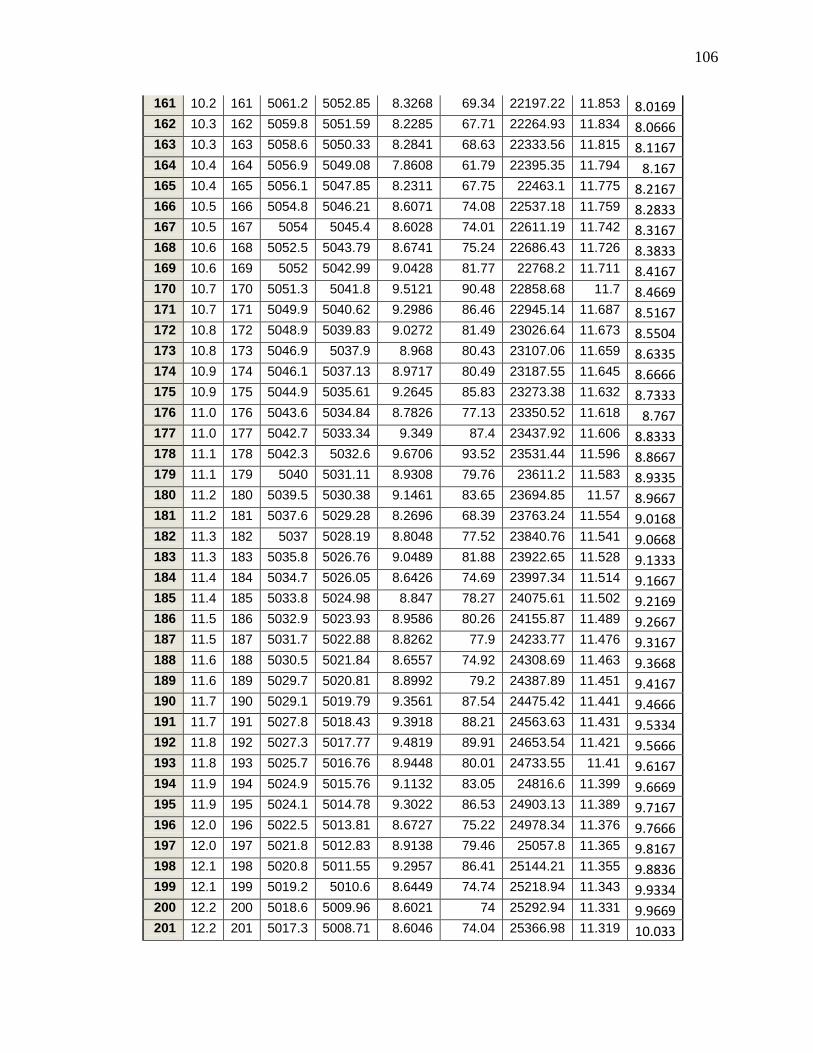
106

161 10.2 161 5061.2 5052.85 8.3268 69.34 22197.22 11.853 8.0169 162 10.3 162 5059.8 5051.59 8.2285 67.71 22264.93 11.834 8.0666 163 10.3 163 5058.6 5050.33 8.2841 68.63 22333.56 11.815 8.1167 164 10.4 164 5056.9 5049.08 7.8608 61.79 22395.35 11.794 8.167 165 10.4 165 5056.1 5047.85 8.2311 67.75 22463.1 11.775 8.2167 166 10.5 166 5054.8 5046.21 8.6071 74.08 22537.18 11.759 8.2833 167 10.5 167 5054 5045.4 8.6028 74.01 22611.19 11.742 8.3167 168 10.6 168 5052.5 5043.79 8.6741 75.24 22686.43 11.726 8.3833 169 10.6 169 5052 5042.99 9.0428 81.77 22768.2 11.711 8.4167 170 10.7 170 5051.3 5041.8 9.5121 90.48 22858.68 11.7 8.4669 171 10.7 171 5049.9 5040.62 9.2986 86.46 22945.14 11.687 8.5167 172 10.8 172 5048.9 5039.83 9.0272 81.49 23026.64 11.673 8.5504 173 10.8 173 5046.9 5037.9 8.968 80.43 23107.06 11.659 8.6335 174 10.9 174 5046.1 5037.13 8.9717 80.49 23187.55 11.645 8.6666 175 10.9 175 5044.9 5035.61 9.2645 85.83 23273.38 11.632 8.7333 176 11.0 176 5043.6 5034.84 8.7826 77.13 23350.52 11.618 8.767 177 11.0 177 5042.7 5033.34 9.349 87.4 23437.92 11.606 8.8333 178 11.1 178 5042.3 5032.6 9.6706 93.52 23531.44 11.596 8.8667 179 11.1 179 5040 5031.11 8.9308 79.76 23611.2 11.583 8.9335 180 11.2 180 5039.5 5030.38 9.1461 83.65 23694.85 11.57 8.9667 181 11.2 181 5037.6 5029.28 8.2696 68.39 23763.24 11.554 9.0168 182 11.3 182 5037 5028.19 8.8048 77.52 23840.76 11.541 9.0668 183 11.3 183 5035.8 5026.76 9.0489 81.88 23922.65 11.528 9.1333 184 11.4 184 5034.7 5026.05 8.6426 74.69 23997.34 11.514 9.1667 185 11.4 185 5033.8 5024.98 8.847 78.27 24075.61 11.502 9.2169 186 11.5 186 5032.9 5023.93 8.9586 80.26 24155.87 11.489 9.2667 187 11.5 187 5031.7 5022.88 8.8262 77.9 24233.77 11.476 9.3167 188 11.6 188 5030.5 5021.84 8.6557 74.92 24308.69 11.463 9.3668 189 11.6 189 5029.7 5020.81 8.8992 79.2 24387.89 11.451 9.4167 190 11.7 190 5029.1 5019.79 9.3561 87.54 24475.42 11.441 9.4666 191 11.7 191 5027.8 5018.43 9.3918 88.21 24563.63 11.431 9.5334 192 11.8 192 5027.3 5017.77 9.4819 89.91 24653.54 11.421 9.5666 193 11.8 193 5025.7 5016.76 8.9448 80.01 24733.55 11.41 9.6167 194 11.9 194 5024.9 5015.76 9.1132 83.05 24816.6 11.399 9.6669 195 11.9 195 5024.1 5014.78 9.3022 86.53 24903.13 11.389 9.7167 196 12.0 196 5022.5 5013.81 8.6727 75.22 24978.34 11.376 9.7666 197 12.0 197 5021.8 5012.83 8.9138 79.46 25057.8 11.365 9.8167 198 12.1 198 5020.8 5011.55 9.2957 86.41 25144.21 11.355 9.8836 199 12.1 199 5019.2 5010.6 8.6449 74.74 25218.94 11.343 9.9334 200 12.2 200 5018.6 5009.96 8.6021 74 25292.94 11.331 9.9669 201 12.2 201 5017.3 5008.71 8.6046 74.04 25366.98 11.319 10.033

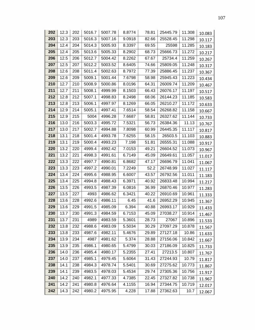
107

202 12.3 202 5016.7 5007.78 8.8774 78.81 25445.79 11.308 10.083 203 12.3 203 5016.3 5007.16 9.0918 82.66 25528.45 11.298 10.117 204 12.4 204 5014.3 5005.93 8.3397 69.55 25598 11.285 10.183 205 12.4 205 5013.6 5005.33 8.2902 68.73 25666.73 11.272 10.217 206 12.5 206 5012.7 5004.42 8.2262 67.67 25734.4 11.259 10.267 207 12.5 207 5012.2 5003.52 8.6405 74.66 25809.05 11.248 10.317 208 12.6 208 5011.4 5002.63 8.7972 77.39 25886.45 11.237 10.367 209 12.6 209 5009.1 5001.44 7.6798 58.98 25945.43 11.223 10.434 210 12.7 210 5008.9 5000.86 8.0196 64.31 26009.74 11.209 10.467 211 12.7 211 5008.1 4999.99 8.1503 66.43 26076.17 11.197 10.517 212 12.8 212 5007.1 4998.83 8.2498 68.06 26144.23 11.185 10.583 213 12.8 213 5006.1 4997.97 8.1269 66.05 26210.27 11.172 10.633 214 12.9 214 5005.1 4997.41 7.6514 58.54 26268.82 11.158 10.667 215 12.9 215 5004 4996.28 7.6687 58.81 26327.62 11.144 10.733 216 13.0 216 5003.3 4995.72 7.5321 56.73 26384.36 11.13 10.767 217 13.0 217 5002.7 4994.88 7.8098 60.99 26445.35 11.117 10.817 218 13.1 218 5001.4 4993.78 7.6255 58.15 26503.5 11.103 10.883 219 13.1 219 5000.4 4993.23 7.198 51.81 26555.31 11.088 10.917 220 13.2 220 4999.4 4992.42 7.0153 49.21 26604.52 11.073 10.967 221 13.2 221 4998.3 4991.61 6.7149 45.09 26649.61 11.057 11.017 222 13.3 222 4997.7 4990.81 6.8682 47.17 26696.79 11.041 11.067 223 13.3 223 4997.2 4990.01 7.2249 52.2 26748.99 11.027 11.117 224 13.4 224 4995.6 4988.95 6.6007 43.57 26792.56 11.011 11.183 225 13.4 225 4994.8 4988.43 6.3971 40.92 26833.48 10.994 11.217 226 13.5 226 4993.5 4987.39 6.0816 36.99 26870.46 10.977 11.283 227 13.5 227 4993 4986.62 6.3421 40.22 26910.69 10.961 11.333 228 13.6 228 4992.6 4986.11 6.45 41.6 26952.29 10.945 11.367 229 13.6 229 4991.5 4985.09 6.394 40.88 26993.17 10.929 11.433 230 13.7 230 4991.3 4984.59 6.7153 45.09 27038.27 10.914 11.467 231 13.7 231 4989 4983.59 5.3601 28.73 27067 10.896 11.533 232 13.8 232 4988.6 4983.09 5.5034 30.29 27097.29 10.878 11.567 233 13.8 233 4987.6 4982.11 5.4676 29.89 27127.18 10.86 11.633 234 13.9 234 4987 4981.62 5.374 28.88 27156.06 10.842 11.667 235 13.9 235 4986.1 4980.65 5.4799 30.03 27186.09 10.825 11.733 236 14.0 236 4985.4 4980.17 5.2355 27.41 27213.5 10.807 11.767 237 14.0 237 4985.1 4979.45 5.6064 31.43 27244.93 10.79 11.817 238 14.1 238 4984.3 4978.74 5.5401 30.69 27275.62 10.773 11.867 239 14.1 239 4983.5 4978.03 5.4534 29.74 27305.36 10.756 11.917 240 14.2 240 4982.1 4977.33 4.7385 22.45 27327.82 10.738 11.967 241 14.2 241 4980.8 4976.64 4.1155 16.94 27344.75 10.719 12.017 242 14.3 242 4980.2 4975.95 4.228 17.88 27362.63 10.7 12.067

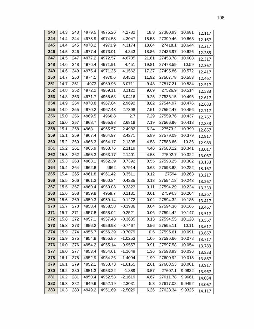
108

243 14.3 243 4979.5 4975.26 4.2782 18.3 27380.93 10.681 12.117 244 14.4 244 4978.9 4974.58 4.3047 18.53 27399.46 10.663 12.167 245 14.4 245 4978.2 4973.9 4.3174 18.64 27418.1 10.644 12.217 246 14.5 246 4977.4 4973.01 4.343 18.86 27436.97 10.626 12.283 247 14.5 247 4977.2 4972.57 4.6705 21.81 27458.78 10.608 12.317 248 14.6 248 4976.4 4971.91 4.451 19.81 27478.59 10.59 12.367 249 14.6 249 4975.4 4971.25 4.1562 17.27 27495.86 10.572 12.417 250 14.7 250 4974.1 4970.6 3.4523 11.92 27507.78 10.553 12.467 251 14.7 251 4973 4969.96 3.0711 9.43 27517.21 10.534 12.517 252 14.8 252 4972.2 4969.11 3.1122 9.69 27526.9 10.514 12.583 253 14.8 253 4971.7 4968.68 3.0416 9.25 27536.15 10.495 12.617 254 14.9 254 4970.8 4967.84 2.9692 8.82 27544.97 10.476 12.683 255 14.9 255 4970.2 4967.43 2.7398 7.51 27552.47 10.456 12.717 256 15.0 256 4969.5 4966.8 2.7 7.29 27559.76 10.437 12.767 257 15.0 257 4968.7 4965.98 2.6818 7.19 27566.96 10.418 12.833 258 15.1 258 4968.1 4965.57 2.4982 6.24 27573.2 10.399 12.867 259 15.1 259 4967.4 4964.97 2.4271 5.89 27579.09 10.379 12.917 260 15.2 260 4966.3 4964.17 2.1395 4.58 27583.66 10.36 12.983 261 15.2 261 4965.9 4963.76 2.1119 4.46 27588.12 10.341 13.017 262 15.3 262 4965.3 4963.17 2.1401 4.58 27592.7 10.322 13.067 263 15.3 263 4963.1 4962.39 0.7392 0.55 27593.25 10.302 13.133 264 15.4 264 4962.8 4962 0.7914 0.63 27593.88 10.282 13.167 265 15.4 265 4961.8 4961.42 0.3511 0.12 27594 10.263 13.217 266 15.5 266 4961.3 4960.84 0.4235 0.18 27594.18 10.243 13.267 267 15.5 267 4960.4 4960.08 0.3323 0.11 27594.29 10.224 13.333 268 15.6 268 4959.8 4959.7 0.1181 0.01 27594.3 10.204 13.367 269 15.6 269 4959.3 4959.14 0.1272 0.02 27594.32 10.185 13.417 270 15.7 270 4958.4 4958.58 -0.1936 0.04 27594.36 10.166 13.467 271 15.7 271 4957.8 4958.02 -0.2521 0.06 27594.42 10.147 13.517 272 15.8 272 4957.1 4957.48 -0.3635 0.13 27594.55 10.128 13.567 273 15.8 273 4956.2 4956.93 -0.7467 0.56 27595.11 10.11 13.617 274 15.9 274 4955.7 4956.39 -0.7079 0.5 27595.61 10.091 13.667 275 15.9 275 4954.8 4955.85 -1.0253 1.05 27596.66 10.073 13.717 276 16.0 276 4954.2 4955.14 -0.9557 0.91 27597.58 10.054 13.783 277 16.0 277 4953.4 4954.61 -1.1649 1.36 27598.93 10.036 13.833 278 16.1 278 4952.9 4954.26 -1.4094 1.99 27600.92 10.018 13.867 279 16.1 279 4952.1 4953.73 -1.6165 2.61 27603.53 10.001 13.917 280 16.2 280 4951.3 4953.22 -1.889 3.57 27607.1 9.9832 13.967 281 16.2 281 4950.4 4952.53 -2.1619 4.67 27611.78 9.9661 14.034 282 16.3 282 4949.9 4952.19 -2.3031 5.3 27617.08 9.9492 14.067 283 16.3 283 4949.2 4951.69 -2.5029 6.26 27623.34 9.9325 14.117

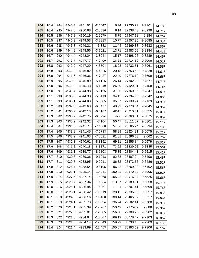
109

284 16.4 284 4948.4 4951.01 -2.6347 6.94 27630.29 9.9161 14.183 285 16.4 285 4947.8 4950.68 -2.8536 8.14 27638.43 9.8999 14.217 286 16.5 286 4947.2 4950.19 -2.9579 8.75 27647.18 9.884 14.267 287 16.5 287 4946.3 4949.53 -3.2813 10.77 27657.95 9.8685 14.334 288 16.6 288 4945.8 4949.21 -3.382 11.44 27669.38 9.8532 14.367 289 16.6 289 4944.9 4948.56 -3.7021 13.71 27683.09 9.8384 14.433 290 16.7 290 4944.4 4948.24 -3.8944 15.17 27698.26 9.8239 14.467 291 16.7 291 4943.7 4947.77 -4.0409 16.33 27714.59 9.8098 14.517 292 16.8 292 4942.9 4947.29 -4.3504 18.93 27733.51 9.7961 14.567 293 16.8 293 4942.3 4946.82 -4.4925 20.18 27753.69 9.7828 14.617 294 16.9 294 4941.6 4946.36 -4.7427 22.49 27776.19 9.7699 14.667 295 16.9 295 4940.8 4945.89 -5.1125 26.14 27802.33 9.7577 14.717 296 17.0 296 4940.2 4945.43 -5.1949 26.99 27829.31 9.7458 14.767 297 17.0 297 4939.4 4944.98 -5.6165 31.55 27860.86 9.7347 14.817 298 17.1 298 4938.5 4944.38 -5.8413 34.12 27894.98 9.7242 14.883 299 17.1 299 4938.1 4944.08 -5.9385 35.27 27930.24 9.7139 14.917 300 17.2 300 4937.3 4943.63 -6.3477 40.29 27970.54 9.7045 14.967 301 17.2 301 4936.7 4943.19 -6.5167 42.47 28013.01 9.6955 15.017 302 17.3 302 4935.9 4942.75 -6.8994 47.6 28060.61 9.6875 15.067 303 17.3 303 4935.2 4942.32 -7.104 50.47 28111.07 9.6801 15.117 304 17.4 304 4934.3 4941.74 -7.4068 54.86 28165.94 9.6734 15.183 305 17.4 305 4933.8 4941.45 -7.6733 58.88 28224.81 9.6675 15.217 306 17.5 306 4933.2 4941.03 -7.8621 61.81 28286.63 9.662 15.267 307 17.5 307 4932.3 4940.61 -8.3192 69.21 28355.84 9.6579 15.317 308 17.6 308 4931.6 4940.18 -8.5571 73.22 28429.06 9.6545 15.367 309 17.6 309 4931.1 4939.77 -8.6803 75.35 28504.41 9.6515 15.417 310 17.7 310 4930.3 4939.36 -9.1013 82.83 28587.24 9.6498 15.467 311 17.7 311 4929.7 4938.95 -9.2911 86.32 28673.56 9.6486 15.517 312 17.8 312 4928.7 4938.54 -9.8195 96.42 28769.99 9.6492 15.567 313 17.8 313 4928.1 4938.14 -10.041 100.83 28870.82 9.6505 15.617 314 17.9 314 4927.5 4937.74 -10.268 105.42 28976.24 9.6525 15.667 315 17.9 315 4926.7 4937.34 -10.634 113.07 29089.31 9.6558 15.717 316 18.0 316 4926.1 4936.94 -10.867 118.1 29207.41 9.6599 15.767 317 18.0 317 4925.1 4936.42 -11.319 128.12 29335.53 9.6657 15.833 318 18.1 318 4924.8 4936.16 -11.408 130.14 29465.67 9.6717 15.867 319 18.1 319 4924.1 4935.78 -11.694 136.74 29602.41 9.6788 15.917 320 18.2 320 4923.1 4935.39 -12.267 150.49 29752.9 9.688 15.967 321 18.2 321 4922.5 4935.01 -12.505 156.38 29909.28 9.6982 16.017 322 18.3 322 4921.6 4934.64 -13.007 169.19 30078.47 9.7103 16.067 323 18.3 323 4921.5 4934.14 -12.649 159.99 30238.45 9.7209 16.133 324 18.4 324 4921.4 4933.89 -12.453 155.07 30393.52 9.7306 16.167

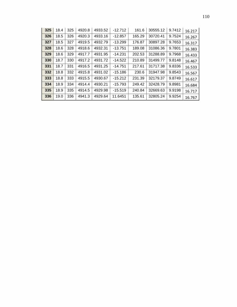
110

325 18.4 325 4920.8 4933.52 -12.712 161.6 30555.12 9.7412 16.217 326 18.5 326 4920.3 4933.16 -12.857 165.29 30720.41 9.7524 16.267 327 18.5 327 4919.5 4932.79 -13.299 176.87 30897.28 9.7653 16.317 328 18.6 328 4918.6 4932.31 -13.751 189.08 31086.36 9.7801 16.383 329 18.6 329 4917.7 4931.95 -14.231 202.53 31288.89 9.7968 16.433 330 18.7 330 4917.2 4931.72 -14.522 210.89 31499.77 9.8148 16.467 331 18.7 331 4916.5 4931.25 -14.751 217.61 31717.38 9.8336 16.533 332 18.8 332 4915.8 4931.02 -15.186 230.6 31947.98 9.8543 16.567 333 18.8 333 4915.5 4930.67 -15.212 231.39 32179.37 9.8749 16.617 334 18.9 334 4914.4 4930.21 -15.793 249.42 32428.79 9.8981 16.684 335 18.9 335 4914.5 4929.98 -15.519 240.84 32669.63 9.9198 16.717 336 19.0 336 4941.3 4929.64 11.6451 135.61 32805.24 9.9254 16.767

111

REFERENCES

Allen T. and Roberts A. (1982),”Production Operations: Well Completion, Workover and

Stimulation,” vol 2 3rd

ed. Oil and Gas Consultants International, Inc. Tulsa

ASTM ,”Standard test method for the determination of the in situ stress in rock using the

hydraulic fracturing method,” Designation D 4645 – 87 (Reapproved 1997)

Antoci, J. C. and Anaya, L. A. (2001),” First Massive Hydraulic Fracturing Treatment in

Argentina,” SPE 69581.

Baree, R.D.,and Mukherjee, H. (1996),”Determination of Pressure Dependent Leak-off

and Its Effect on Fracture Geometry,” SPE 36424.

Branagan, P.T. and Holzhausen, G.R. (1994),”Applied Geomechanics Inc. Improvements

in Defining the Magnitude of the Minimum In-Situ Stress Using Hydraulic

Impedance Testing and Pressure Derivative Analysis,” SPE 27898

Castillo, J.L. (1987),”Modified Fracture Pressure Decline Analysis Including Pressure-

Dependent Leakoff,” SPE 16417

Daneshy, A.A., Slusher,G.L.,Chilholm, P.T. and Magee, D.A. (1986),”In-Situ Stress

Measurements During Drilling,” JPT, Vol 38, No. 9.

deBree, P. and Walters, J.V. (1989),”Micro/Mini-frac Test Procedures and Interpretation

for In-situ Stress Determination,” international Journal of Rock Mechanics and

Mining Sciences, Pergamon Press, Vol. 26 No.6.

Doe, T.W. and Korbin, G.E. (1987),”A comparison of hydraulic fracturing and hydraulic

jacking stress measurements,” ARMA 87-0283.

Economides, M.J. and Nolte, K.G. (2000),”Reservoir Stimulation,” 3rd

edition ISBN 0

471 49192 6, Schlumberger Dowell, Sugar Land, Texas.

Gu, H. and Leung, K.H. (1993),”3D Numerical Simulation of Hydraulic Fracture Closure

With Application to Minifracture Analysis,” SPE 20657-PA.

Haimson, B.C. (1974),”A simple method for estimating in-situ stresses at greater depths,”

Field Testing and Instrumentation of Rock, ASTM STP 554, American Society

for Testing of Materials, pp 156-182.

Hallahan, C. and Atkinson, L.,”Introduction to using SAS EG for Statistical analysis,”

Paper 117-29.

112

Holt, R.M., Pestman, B.J. and Kenter, J. (2001),”Use of a discrete particle model to

assess feasibility of core based stress determination,” ISBN 90 2651 827 7.

Hubbert, M.K. and Willis, D. G. (1957),” Mechanics of Hydraulic Fracturing,” Trans,

AIME, Vol . No. 210.

Jackson, C.W.,”SAS Programming basics,” CSQA.

Jones, J. and Britt, L. (2009).”Design and Appraisal of Hydraulic Fractures,” ISBN 978-

1-5563-143-7, Society of Petroleum Engineers, Richardson, TX.

Lee, M.Y. and Haimson, B.C. (1989),”Statistical Evaluation of Hydraulic Fracturing

Stress Measurement Parameters,” International Journal of Rock Mechanics, Min.

Sci. And Geomech. Abstr., Vol. 26, No. 6 pp. 447-456.

Lin, P. and Ray, T.G. (1996),”A New Method for Direct Measurement of In-Situ Stress

Directions and Formation Rock Properties” SPE 26600 – PA.

Martins, C. S., Ribiero, L. and Sousa, E. (1987),”Recent advances in the interpretation of

the small flat jack method,” ISRM 6CONGRESS-1987-230.

McLennan, J. D. and Roegiers, J.C. (1982),”How instantaneous are instantaneous

pressures,” SPE 11064.

Mohamed, I.M., Nasralla, R.A., Sayed, M.A., Marongiu-Porcu, M., and Ehlig, C.A. –

Economides (2011),”Evaluation of After Closure Analysis for Tight and Shell

Gas Formations,” SPE 140136.

Nawrocki, P. A. (2010),”Critical Wellbore Pressures Using Different Rock Failure

Criteria.”

Nolte, K.G. (1988),”Application of Fracture Design Based on Pressure Analysis” SPE

Production Engineering.

Nolte, K.G. amd Smith, M.B. (1981),”Interpretation of Fracturing Pressures,” SPE 8297

SAS Institute Inc.,”SAS enterprise guide 4.2.”

“SAS Online Doc Version 8,”

http://ciser.cornell.edu/sasdoc/saspdf/common/mainpdf.htm, Sept 2012

Smith, M.B., Holman, G.B., Fast, C.R., and Covlin, R.J. (1978),”The Azimuth of Deep,

Penetrating Fractures in The Wattenberg Field ,” SPE 6092 – PA

Siegfried, R. W., and Simmons, G. (1978), "Characterization of Oriented Cracks with

Differential Strain Analysis," J. Geoph. Res 83.(B3), 1269-1278.

113

Soliman, M.Y., and Daneshy, A.A. (1991),”Determination of Fracture Volume and

Closure Pressure From Pump ln/Flowback Tests,” SPE 21400.

Simmons, G., and Richter, D., (1976), "Microcracks in Rocks," The Physics and

Chemistry of Minerals and Rocks (R.G.J Strens, ed.), Interscience, New York, pp

105-137.

Thompson, J.W. and Church, D.C. (1993),”Design, Execution, and Evaluation of

Minifracs in the Field: A Practical Approach and Case Study,” SPE 26034.

Upchurch, E.R. (1993),”Determining Fracture Closure Pressure In Soft Formations Using

Postclosure Pulse Testing” SPE 56723.

van Dam, D.B. and de Pater, C.J. (1996),”Roughness of Hydraulic Fractures: The

Importance of In-Situ Stress and Tip Processes” SPE 56596.

van Dam, D.B., de Pater, C.J. and Romijn, R. (1998),”Analysis of Hydraulic Fracture

Closure in Laboratory Experiments” SPE/ISRM 47380.

Warpinski, N. R., and Smith, M.B. (1982),“Rock Mechanics and Fracture Geometry,” in

Recent Advances in Hydraulic Fracturing, SPE Monograph, 12, p. 57-80.

Warpinski, N. R., Branagan, P.T. and Wilmer, R. (1983),”In-situ Stress Measurements at

DOE‟s Multiwell Equipment Site,” SPE 12142 - 58.

Warpinski, N.R., Clark, J.A., Schmidt, R.A., Huddle, C.W. (1982),”Laboratory

Investigation on the Effect of In Situ Stresses on Hydraulic Fracturing

Containment,” SPE 9834 – PA.

Weng, X., Pandey, V., and Nolte, K.G. (2002), “Equilibrium Test – A Method for

Closure Pressure Determination” SPE/ISRM 78173.

Wright, C.A., Weigers, L., and Minner, W.A. (1996),”Robust Technique For Real-Time

Closure Stress Determination” SPE Production and Facilities.

114

VITA

Soumitra Bhaskar Nande was born in Pune, Maharashtra, India. He received his

primary and secondary education in Pune, India graduating from Bharat English School

and Junior College in 2006. Soumitra received a Bachelor of Engineering degree in

Petroleum Engineering from Maharashtra Institute of Technology, affiliated to University

of Pune in May 2010. He received a Master of Science degree in Petroleum Engineering

from Missouri University of Science and Technology, Rolla, Missouri in May 2013.