COMPARISON OF RAY TRACING THROUGH IONOSPHERIC · PDF filecomparison of ray tracing through...
94
COMPARISON OF RAY TRACING THROUGH IONOSPHERIC MODELS THESIS Shayne C. Aune, Second Lieutenant, USAF AFIT/GE/ENG/06-04 DEPARTMENT OF THE AIR FORCE AIR UNIVERSITY AIR FORCE INSTITUTE OF TECHNOLOGY Wright-Patterson Air Force Base, Ohio APPROVED FOR PUBLIC RELEASE; DISTRIBUTION UNLIMITED
Transcript of COMPARISON OF RAY TRACING THROUGH IONOSPHERIC · PDF filecomparison of ray tracing through...

COMPARISON OF RAY TRACING
THROUGH IONOSPHERIC MODELS
THESIS
Shayne C. Aune, Second Lieutenant, USAF
AFIT/GE/ENG/06-04
DEPARTMENT OF THE AIR FORCE AIR UNIVERSITY
AIR FORCE INSTITUTE OF TECHNOLOGY
Wright-Patterson Air Force Base, Ohio
APPROVED FOR PUBLIC RELEASE; DISTRIBUTION UNLIMITED

The views expressed in this thesis are those of the author and do not reflect the official policy or position of the United States Air Force, Department of Defense, or the United States Government.
ii

AFIT/GE/ENG/06-04
COMPARISON OF RAY TRACING THROUGH IONOSPHERIC MODELS
THESIS
Presented to the Faculty
Department of Systems and Engineering Management
Graduate School of Engineering and Management
Air Force Institute of Technology
Air University
Air Education and Training Command
In Partial Fulfillment of the Requirements for the
Degree of Master of Science in Electrical Engineering
Shayne C. Aune, B.S.E.E.
Second Lieutenant, USAF
March 2006
APPROVED FOR PUBLIC RELEASE; DISTRIBUTION UNLIMITED.
iii

AFIT/GE/ENG/06-04
COMPARISON OF RAY TRACING THROUGH IONOSPHERIC MODELS
Shayne C. Aune, B.S.E.E. Second Lieutenant, USAF
Approved: ______________/signed/________________ 3 Mar 06 Lt Col Matthew E. Goda, PhD (Chairman) date ______________/signed/________________ 3 Mar 06 Dr. William S. Borer (Member) date ______________/signed/________________ 6 Mar 06 Dr. Ronald F. Tuttle (Member) date ______________/signed/________________ 6 Mar 06 Maj Christopher G. Smithtro, PhD (Member) date
iv

AFIT/GE/ENG/06-04 Abstract
A comparison of ray tracing predictions for transionospheric electromagnetic wave refraction
and group delays through ionospheric models is presented. Impacted applications include over-
the-horizon RADAR, high frequency communications, direction finding, and satellite
communications. The ionospheric models used are version 2.1 of Utah State University's Global
Assimilation of Ionospheric Measurements (USU GAIM) model and the 2001 version of the
International Reference Ionosphere (IRI) model. In order to provide ray tracing results
applicable to satellite communications for satellites at geosynchronous orbit (GEO), a third
ionospheric model is used to extend the sub-2000-km USU GAIM and IRI ionospheric
specifications to 36540 km in altitude. The third model is based on an assumption of diffusive
equilibrium for ion species above 2000 km. The ray-tracing code used is an updated
implementation of the Jones-Stephenson ray-tracing algorithm provided by L. J. Nickisch and
Mark A. Hausman. Ray-tracing predictions of signal refraction and group delay are given for
paths between Goldstone Deep Space Observatory near Barstow, California, and the PanAmSat
Galaxy 1R satellite. Results are given for varying frequency between 11MHz to 1GHz, varying
time of day between 0600 and 1700 Pacific Standard Time on 1 November 2004, and varying
signal transmission elevation angle. Ray tracing predicts minimal ionospheric effects on signals
at or above approximately 100 MHz. Ray-tracing predictions of signal refraction and group
delay differ dependent upon the model used for ray-tracing. Ray tracing in diffusive equilibrium
extended (DEE) USU GAIM (DEE GAIM) predicts as much as 500 km less group path length
than DEE IRI. This is most likely due to the DEE model propagating high electron densities
found in the upper altitudes of IRI-2001 specifications. USU GAIM ray tracing predicts higher
frequencies are necessary to penetrate the F2 region during the period of interest than IRI-2001.
v

AFIT/GE/ENG/06-04
To My True Love
vi

Acknowledgments
GOD REIGNS. I stand beside the believers who acknowledge a thesis is accomplished
by love, persistence, and sacrifice, not only from self, but by all those whom love the author
most dearly. This work is first and foremost accomplished by GOD’s intervention. FATHER, I
pray YOUR hands continue to lift up all who seek YOUR enlightenment through lifelong study
and devotion to understanding YOUR creation.
Second only to God is my family. To my True Love, to our Lord’s most wonderful gifts,
our children, and to my mother, father, brothers, and sisters: I devote this work to all of you.
There are no words to express my gratitude for the love you have given and sacrifices you have
made allowing me to become a Master. I will always love you and seek to empower you as you
have empowered me to achieve this milestone.
I would also like to express my deep appreciation to the many people who went out of
their way to assist in my development, guiding this research. To my advisor and sponsor, Dr.
William Borer, for your patience and support from afar; it is no easy task taking on a master’s
student with an already completely full schedule. I have no idea how you did it, but I realize you
went way out on a limb to help me achieve beyond my own wildest research expectations.
Thank You. To my AFIT advisor, Lt Col Matt Goda, thank you, sir, for your enduring support,
for your MATLAB coding expertise, and for keeping the pressure to a minimum while keeping
me on task to accomplish something rarely (if ever) done here before: a “stand-alone” AND an
addendum. Thank you, Dr. Ronald Tuttle, for agreeing at practically the last minute to help with
this effort, and for always being the first to read and provide feedback on my many thesis drafts.
And, Thank you, Maj Christopher Smithtro, for your ionospheric expertise and always being
ready to provide immediate feedback and recommendations on how to proceed into this
churning, mysterious, and amazing medium!
vii
I am also indebted to the many professionals who spent their valuable time carefully
instructing me in the science of ionospheric modeling and ray tracing. Thank you, Dr. L. J.
Nickisch, for introducing me to the theory and history of ray tracing. Thank you, Dr. Mark
Hausman, for your expertise and recommendations in implementing and displaying ray tracing
results using numerous computer applications. Thank you, Maj Herbert Keyser and Capt Craig
Baker for providing the multitude of USU GAIM specifications required. Thank you, Dr. Don
Thompson, for your USU GAIM model expertise, and thank you, Dr. Dieter Bilitza, for your IRI
model expertise.
Thank you, Craig Miller, Don Soulliere, Anthony Virgilio, and Pat Dolan, for getting
operations going on both sides of the wall so I could explore a new frontier! Your good humor
and patience kept me sane when it came down to the wire. Thank you, my fellow AFIT masters
students, especially Lt Jared Herweg, Capt Drew Hyatt, Capt Evan James, Maj Chris Lemanski,
Lt John MacDonald, Lt Becky Eckert, Capt Neil Paris, Lt Steve Mawhorter, Lt Willie Mims, and
all the rest. We made it together! May God continue to bless us!
Thank you, John Hando, Dr. Tom Brehm, Lt Col Kevin Allen, Capt William Sacovitch,
Capt Michael Pratt, Dr. William Frix, and Will Sturgis for your support from NASIC. Thank
you also, Dr. Andrew Terzuoli, Dr. John Raquet, and Lt Col Stewart DeVilbiss at AFIT, for your
help and guidance along this winding path. Thank you, Mr. Al Gifford and Lt Col James Bolles,
for your approval and support of this research effort. And, finally, THANK YOU, Lt Col Eric
Claunch, for leading, mentoring, and providing me with the network to help pave the road for
future students at AFIT. You passed the torch and ensured my success from the beginning.
MISSION ACCOMPLISHED, SIR!
/signed/ Shayne Christopher Aune
viii

Table of Contents
Page Abstract ................................................................................................................................... v Dedication ................................................................................................................................ vi Acknowledgements ................................................................................................................. vii Table of Contents ................................................................................................................... ix List of Figures ........................................................................................................................ xi List of Tables ........................................................................................................................ xii
I. Introduction ........................................................................................................................ 1 General Issue ...................................................................................................................... 1 Overview ............................................................................................................................ 2 Results Preview .................................................................................................................. 4 II. Background........................................................................................................................ 5 The Ionosphere .................................................................................................................. 5 Signal Propagation in the Ionosphere................................................................................ 9 Raytracing ....................................................................................................................... 16 Ionospheric Models ......................................................................................................... 20 III. Methodology ................................................................................................................... 25 Overview ........................................................................................................................ 25 The Models...................................................................................................................... 27 The Raytracing Algorithm............................................................................................... 33 MATLAB®..................................................................................................................... 34 IV. Results............................................................................................................................. 35 Overview ......................................................................................................................... 35 TEC Maps ....................................................................................................................... 36 Ray Refraction................................................................................................................. 45 Angular Deviation ........................................................................................................... 49 Signal Group Path ........................................................................................................... 56 V. Conclusion........................................................................................................................ 59 Summary ......................................................................................................................... 59 Future Research............................................................................................................... 61 Appendix A. IRI Model Specification Input and Output Example ....................................... 63 Appendix B. MATLAB m-Files............................................................................................ 64 FullTECPlot.m ................................................................................................................ 64
ix
GAIM4mat_extend.m...................................................................................................... 66 RayOutput.m ................................................................................................................... 68 RaytraceOut.m................................................................................................................. 70 Appendix C. Ray Tracing Algorithm Input and Output Examples ....................................... 72 Appendix D. Variable DEE IRI Grid-Spacing Effects on Ray-Tracing Predictions ............. 76 Appendix E. Attempted USU GAIM Model Specification Extrapolation............................. 78 Bibliography.......................................................................................................................... 79 Vita........................................................................................................................................ 81
x
List of Figures
Figure Page 2.1. Ionospheric Electron Density Profile Showing Regions ................................................. 6 2.2. Ionospheric TEC Variability ........................................................................................... 8 2.3. Snell’s Law.................................................................................................................... 11 2.4. Frequency- and Electron Density-Dependence of Index of Refraction......................... 11 2.5. A Real-Time Ionogram ................................................................................................. 13 2.6. Comparison of Ray-Traced Ionospheric Path versus Straight-Line Path ...................... 14 2.7. 10_MHz Signal Ionospheric Refaction as a Function of Angle of Incidence ............... 15 2.8. Spherical Polar Coordinates Relative to Cartesian Coordinates.................................... 19 3.1. Methodology Process .................................................................................................... 26 3.2. Diffusive Equilibrium Extended (DEE) IRI Ionospheric Profile .................................. 29 3.3. DEE GAIM Ionospheric Profile .................................................................................... 31 3.4. Comparison of DEE IRI and DEE GAIM Ionospheric Profiles .................................... 32 4.1. IRI-2001 TEC Map at 0600 PST................................................................................... 38 4.2. USU GAIM 2.1 TEC Map at 0600 PST........................................................................ 38 4.3. IRI-2001 TEC Map at 1400 PST................................................................................... 40 4.4. USU GAIM 2.1 TEC Map at 1400 PST........................................................................ 40 4.5. IRI-GAIM TEC Difference Map at 1400 PST .............................................................. 41 4.6. DEE IRI TEC Map at 1400 PST ................................................................................... 43 4.7. DEE GAIM TEC Map at 1400 PST .............................................................................. 43 4.8. DEE IRI-DEE GAIM TEC Difference Map at 1400 PST............................................. 44 4.9. Varying Elevation Ray Refraction for 11-14 MHz thru DEE IRI at 1400 PST ............ 46 4.10. Varying Elevation Ray Refraction for 11-14 MHz thru DEE GAIM at 1400 PST ....... 46 4.11. Varying Elevation 11-14 MHz Crossrange Ray Refraction thru DEE IRI at 1400 PST............................................................................................ 48 4.12. Varying Elevation 11-14 MHz Crossrange Ray Refraction thru DEE IRI at 1400 PST............................................................................................ 48 4.13. Elevation Deviation vs Time of Day for 15-1000 MHz thru DEE IRI.......................... 50
xi
4.14. Elevation Deviation vs Time of Day for 15-1000 MHz thru DEE GAIM .................... 50 4.15. Target Miss Distance for Angle Deviation.................................................................... 51 4.16. Azimuth Deviation vs Time of Day for 15-1000 MHz thru DEE IRI ........................... 54 4.17. Azimuth Deviation vs Time of Day for 15-1000 MHz thru DEE GAIM...................... 54 4.18. Azimuth Deviation from LOS Zero Crossing as a Function of Time of Day................ 55 4.19. Group Path vs Time of Day for 15-1000 MHz thru DEE IRI ....................................... 57 4.20. Group Path vs Time of Day for 15-1000 MHz thru DEE GAIM .................................. 57 D.1. Ray-Tracing Predicted Azimuth Deviation for Varying DEE IRI Grid Spacing.......... 76 D.2. Ray-Tracing Predicted Elevation Deviation for Varying DEE IRI Grid Spacing ........ 77 D.3. Ray-Tracing Predicted Group Path Deviation for Varying DEE IRI Grid Spacing ..... 77 E.1. Extrapolated GAIM TEC Map at 0600 PST ................................................................. 78
List of Tables
Table Page 1. Ray-Tracing Equation Symbols ....................................................................................... 18
xii

COMPARISON OF RAY TRACING THROUGH IONOSPHERIC MODELS
I. Introduction
General Issue
Various United States national defense activities are affected by the ionosphere in the
accomplishment of their missions. Satellite communications (SATCOMM) relies on signals
which must propagate through the ionosphere, while over-the-horizon RADAR (OTHR), high
frequency (HF) communications, and target direction finding (DF) require predictable signal
reflection from the ionosphere for effective operations. These activities use signal frequencies
below 1 gigahertz (GHz) and they all benefit by knowledge of the ionospheric state and its
impacts on their signals. Predictions of the ionosphere’s state are typically made using
ionospheric models, which sometimes provide inaccurate estimates resulting in errors to the
above activities. Two of the ionospheric signal effects that cause errors in these activities are
refraction and group path delay (increases to signal group path length). Unpredicted ionospheric
refraction results in deficient antenna aim in SATCOMM and HF leading to sub-optimal
communications. Poor compensation for refraction and group path delays may result in
erroneous target identification and coordinate estimation by OTHR and DF, placing friendly
forces at greater risk of failure to identify, locate, and engage adversaries.
Signal propagation prediction methods, such as three-dimensional ray-tracing algorithms
applied to ionospheric models are used by some national defense activities to estimate and
1

mitigate ionospheric effects on signals. Advancing ionospheric modeling technology may hold
the potential to further reduce errors in activities by providing for more accurate ray-tracing
predictions. However, there are numerous models available, many being updated as technology
improves, and each may be based on differing assumptions, inputs, calculations, and result in
differing outputs.
Very little research has been done to compare ionospheric models and their
appropriateness for obtaining ray-tracing predictions in order to mitigate effects on various
activities’ signals. For instance, ray-tracing prediction for SATCOMM requires the use of
ionospheric model specifications up to geosynchronous orbit (GEO) altitude: where many
communications satellites reside. This thesis will focus on the SATCOMM application and seek
to compare two ionospheric models, extended to GEO by a third ionospheric model, to highlight
the differences in refraction and group path predictions obtained by ray tracing through the
models for transionospheric signals below 1 GHz. The results of this thesis examine some
differences between the models and the differences in predictions obtained by ray tracing
through the models.
Overview
This thesis includes a comparison of vertical total electron content (TEC) maps created
using Utah State University’s Global Assimilation of Ionospheric Measurements (USU GAIM or
GAIM) model, version 2.1, and the 2001 version of the International Reference Ionosphere (IRI-
2001 or IRI) model. This thesis also presents ray-tracing predictions of ionospheric effects on
2

signals below 1 GHz. However, it is critical to highlight before continuing that many of the
results obtained in this thesis are not solely due to IRI and GAIM ionospheric specifications.
Because IRI and GAIM model specifications only extend to 2000 km and 1380 km in altitude
respectively and this thesis seeks to include ray-tracing predictions to GEO in order to be useful
to SATCOMM, most of the model specifications used for ray-tracing in this thesis include a
third ionospheric model, referred to as the diffusive equilibrium extension (DEE) model.
Therefore, many of the ray-tracing predictions shown in this thesis are accomplished by ray
tracing signal paths through DEE IRI and DEE GAIM specifications. DEE IRI and DEE GAIM
ray-tracing predictions are not the results of ray tracing through the IRI and GAIM models.
Only the results obtained by ray tracing through the specifications to altitudes less than the IRI
and GAIM maximum altitudes can be attributed to those models.
Chapter two of this thesis discusses background: the ionosphere, how it theoretically
affects signal propagation, the Jones-Stephenson ray-tracing algorithm, and finally, the
ionospheric models used. Chapter three covers methodology, which is primarily the process of
integrating the major components of this research: the models, the ray-tracing algorithm, and
MATLAB®. Chapter four presents results to include a comparison of model-predicted TEC
maps and ray-tracing predictions of ionospheric signal refraction, angular deviation from line of
sight (LOS) to a target, and group path. Finally, chapter five gives a summary and
recommendations for future research. The next section provides a preview of the results
obtained by this research.
3

Results Preview
GAIM results show more concentrated ionospheric electron density layers during the
period of interest, while IRI predicts lower electron densities, spread over greater volume.
GAIM and IRI TEC maps are on the same order of magnitude, with GAIM maps showing more
intense gradients than IRI. GAIM ray-tracing predictions show higher frequencies are necessary
to penetrate the lower ionosphere than frequencies predicted by ray tracing in IRI. However, IRI
typically predicts higher electron densities than GAIM in the upper altitudes of corresponding
specifications. As a consequence of this and due to the DEE model and extension method used,
the resulting DEE IRI TEC map is an order of magnitude higher than the DEE GAIM TEC map.
Ray tracing through DEE IRI predicts higher angular deviation from the LOS elevation and
azimuth to a satellite receiver from the ground, and longer group path lengths than DEE GAIM.
DEE IRI ray-tracing predictions also appear smoothly varying during the day of 1 November
2004, whereas DEE GAIM results have steeper gradients, i.e. a more “jagged” appearance in the
results than DEE IRI. The differences seen in predictions from ray tracing through DEE IRI and
DEE GAIM indicate an accurate topside ionospheric specification extension is critical to ray-
tracing predictions. Yet, one important similarity found is ray tracing through both extended
model specifications predicts the ionosphere causes minimal refraction and group path effects on
signals at frequencies above approximately 100 MHz. Refer to chapter four for the details of
these results.
4

II. Background
The Ionosphere
The ionosphere is an ionized, highly non-linear, and dynamic medium, formed mainly by
solar energy. It is affected by space and terrestrial weather, and by the Earth’s magnetosphere.
The “boundaries” of the ionosphere depend on the reference consulted, but most seem to agree it
begins at no less than 50 kilometers (km) in altitude and extends into the plasmasphere, the edge
of which is 4-8 Earth radii distance (depending on solar activity). The ionosphere is primarily
formed by the Sun’s extreme ultraviolet (EUV) and soft x-ray radiation breaking atmospheric
molecules into ions and free electrons, known as the photoionization process. This thesis will
focus on the daytime, mid-latitude ionosphere. This segment of the ionosphere may be
subdivided into several regions, or layers: D, E, F1, F2, the topside ionosphere, and the
protonosphere (Schunk, 2000). An illustration of these regions is provided in figure 2.1, which
is generated using a combination of ionospheric models. A detailed description for each region
is beyond the scope of this report, but a summary of each will be given next.
Each ionospheric region is characterized by a peak density typically in a certain altitude
range, each corresponds to a different dominating ion composition, and each is subject to
different processes and rates of ion production and loss. The D region (60 to 100 km) is the most
difficult to observe and describe. It is a complex mixture of both positive and negative ions,
5

102 103 104 105 106101
102
103
104
105
Electron Density, cm-3
Alti
tude
, km
Ionospheric Electron Density Profile Showing Regions
F2
F1ED
TOPSIDE
PROTONOSPHERE
Figure 2.1. A log-log ionospheric electron density versus altitude profile displaying the main regions of the ionosphere, D, E, F1, F2, topside, and the protonosphere. The peak densities will vary in altitude. This figure was generated using the International Reference Ionosphere (IRI) ionospheric model, and extended above 2000 km using a diffusive equilibrium model. numerous neutral species, and water cluster ions. The E region (100 to 150 km) provides the
first ion density peak, and was the first region detected. The major ion species in the E region
are NO+, O2+, and N2+. The F1 region (150 to 250 km) is primarily another transition region, in
which O+ becomes the major ion. O+ remains the major ion throughout the F2 region (250 to
400 km) and in the topside ionosphere (300 to 1000 km). Ion-atom interchange and transport
processes start to become important in F1, and the ionosphere’s peak ion density, which occurs in
6

F2, is the result of a balance between plasma transport and chemical loss processes. The peak
density in F2 is approximately an order of magnitude greater than the peak in the E region.
Beyond this peak is the region called the topside ionosphere, in which the density decays with
increasing altitude. The protonosphere (above 1000 km) is the region where H+ and He+
replace O+ as the dominant ion. In these last two regions, plasma transport is the dominating
process (Schunk and Nagy, 2000). This summary has revealed some of the complexities a
physical description of the ionosphere requires. Further complicating this description are the
cyclical and unpredictable variations described next.
Figure 2.2 displays one measure of the ionosphere’s variability in the form of TEC. The
figure shows TEC (1 TEC = 1016 electrons per square meter) measured on a daily basis over
Hamilton, Massachusetts, for the year of 1989. It provides the observer with a somewhat
predictable pattern. Just before sunrise, TEC begins to increase and peaks between noon and
1400 local time. It then decreases as loss processes, such as chemical recombination, dominate
over production processes, such as photoionization. During the night, ion and free electron
losses continue versus minimal photoionization such that minimum TEC occurs a few hours
before sunrise. Figure 2.2 also alludes to the ionosphere’s seasonal variation, showing TEC
peaks higher in winter than in summer. There are notable day-to-day differences, most likely
due to solar and geomagnetic disturbances, or short-term effects and localized anomalies, such as
traveling ionospheric disturbances (TID). Not apparent here is how the ionosphere also varies
according to the 11-year long solar cycle (from solar maximum to minimum and back to
maximum). All of these ongoing variations hold important consequences for transionospheric
electromagnetic (EM) waves (Misra, 2001).
7

Figure 2.2. Ionospheric TEC variability provides a measure of how the ionosphere varies over Hamilton, Massachusetts during 1989. (One TEC is 1016 electrons per square meter.) Note the day-to-day and seasonal variation (Borer, 2005).
8

Signal Propagation in the Ionosphere
The most well-established ionospheric effects on transionospheric EM signals include
absorption, refraction, phase and group delay, frequency shift, polarization shift, and Faraday
rotation. This thesis focuses on characterizing and analyzing two of these effects: 1) signal
refraction and 2) signal group delay. Both of these effects are related to the ionosphere’s varying
index of refraction which can be directly linked to the free electron content. A simple case is
shown by an EM signal traveling in the vertical direction through a nonmagnetic, ionized
medium. The waves’ phase velocity, u, is related to the speed of light in a vacuum, c, by
2
e2
e
cu = n q1-m fπ
(2.1)
where ne is the electron density in units of electron count per cubic centimeter, q is the
magnitude of the electron charge, me is the mass of the electron in grams, and ƒ is the frequency
of the EM wave (Tascione, p. 113). The refractive index of the medium, μ, is defined as
2
e2
e
n q1-m
cu f
μπ
= = (2.2)
Therefore, as a wave passes from lower to higher electron density regions, the refractive index
affecting the wave decreases, and the wave phase accelerates. Alternatively, as the wave passes
9

from higher to lower electron density, the refractive index affecting the wave increases, and the
wave phase decelerates.
Snell’s Law is given mathematically as
1 1 2sin sin 2μ θ μ θ= (2.3)
where subscripts refer to two adjacent mediums through which an EM wave propagates, and θ is
the angle of propagation in the relevant medium. This law indicates that, as shown in Figure 2.3,
a wave exiting a medium with index of refraction, μ1, at angle θ1 relative to the boundary normal,
is refracted upon entering a medium with index of refraction, μ2, at angle θ2, where θ2 > θ1 when
μ2 < μ1. According to equation 2.2, the index of refraction approaches unity (the point at which
no refraction occurs) when either the wave frequency approaches infinity or when the medium’s
electron density goes to zero, since all other quantities in the relationship are constants. Figure
2.4 provides a visual representation of higher frequencies refracting less in the ionosphere. It
further shows that as electron density decreases, signals also refract less. For the purposes of
this thesis, signals above 1GHz are considered to have no appreciable signal refraction.
Additionally, the group delays of signals above 1GHz will not be studied here because, although
the ionospheric-added group delays are not negligible for the purposes of SATCOMM, plenty of
applicable research is already well-documented and compensation techniques are in common use
by the Global Positioning Satellite (GPS) system (Misra, 2001). This thesis focuses on
ionospheric refraction and group delay on signals at frequencies below 1GHz.
10

Figure 2.3. Snell’s Law indicates that because the ionospheric index of refraction is greater than that of the neutral atmosphere, the signal direction will change to make a greater angle with the normal to the boundary, θ2 > θ1.
Neutral Atmosphere, μ1
Ionosphere, μ2
θ1
θ2
Figure 2.4. The index of refraction is frequency and/or electron density dependent such that as the signal frequency increases and/or electron density decreases, the signal is less refracted.
Neutral Atmosphere
Ionosphere
ƒ1, ne,1
ƒ2, ne,2
ƒ3, ne,3
ƒ1 >ƒ2 >ƒ3 ne,1< ne,2< ne,3
11

Another important relationship can be derived from equation 2.1 by noting that as neq2
approaches πmeƒ2, the phase velocity, u, approaches infinity, at which point the signal’s forward
progression is reversed and the signal is reflected. Substituting in for π, the electron charge
magnitude, and the electron mass provides an equation for when reflection occurs, at the critical
frequency for a known electron density:
39 10r ef n−= × Hz (2.4)
This relationship makes it possible to map the reflective or “bottomside” ionosphere from the
ground, as shown in the ionogram in Figure 2.5.
An ionogram is generated by an ionosonde, which transmits and records the echoes from
vertically-aimed, high frequency radio pulses reflected by the ionosphere. The ionosonde
sweeps the pulses over a range of frequencies to detect varying electron densities, and
determines their corresponding altitudes based upon the time difference between transmission
and echo return. Equation 2.4 relates each frequency to the electron density that reflects it.
Initially, altitudes are calculated by multiplying the assumed signal velocity (free-space
propagation) by the time of signal propagation and dividing by two since the signal propagates
up and back. However, because the signal velocity is not constant (not free-space propagation),
it is necessary to rescale the real-time “virtual” altitude calculation. Computers handle true
height scaling, correcting for lower atmospheric and ionospheric composition, which affects
signal velocity prior to reflection (NGDC/STP, 2004). The scaled, “true” altitude versus
12

frequency is shown in figure 2.5 as the lowest curve spanning the ionogram and increasing from
left to right.
Frequency, MHz
Altitud
e, k
m
Figure 2.5. A real-time ionogram shows a bottomside ionospheric profile of altitude versus frequency. Ionograms are generated by ionosondes, which transmit varying-frequency, vertically aimed radio pulses and record the pulse echoes reflected by the ionosphere. Each echoed frequency identifies an electron density in the ionosphere; higher frequencies penetrate further before being reflected. The upper black curve is at “virtual” altitudes, determined by time difference between each pulse transmission and reception, and the lower black curve is the computer-scaled, true altitude, which takes into account non-linear pulse velocities. Note the highest-altitude returns are assumed to be secondary pulse echoes (NGDC/STP, 2004).
It is important to keep in mind the ionosphere is not a mirror-like shell enclosing the
Earth. It is a dynamic medium through which signals are delayed and refracted prior to being
13

either reflected back towards the Earth, or propagating through the peak electron density into
space. It is also important to remember that whether or not a signal is reflected or penetrates
depends on the angle at which it strikes the ionosphere and the electron content in its path.
Figure 2.6 shows a signal path through an electron density model of the ionosphere versus a
straight-line path. (Note: the LOS path is curved due to flattening of the Earth’s surface to be the
horizontal axis.) The raytraced signal refracts away from vertical propagation as the signal
enters increasingly higher electron density layers, and then refracts back towards vertical
propagation as the signal moves past the maximum density region.
Figure 2.6. Comparison of a ray-traced ionospheric signal path versus a straight-line path. The straight-line path appears curved because it is relative to a flattened Earth (horizontal axis). The electron density refracts the transionospheric signal from what would otherwise be a straight path; first refracting it more towards the Earth’s surface as the electron density increases, and then away as the signal moves into decreasing density (Borer, 2005).
Figure 2.7 shows a 10-MHz signal entering the ionosphere at increasing angles of
incidence. The signal is initially propagated vertical linearly, but as the angle increases it is
increasingly refracted, and then completed reflected by the ionosphere. Further, note that as the
incident angle continues to increase beyond reflection, the signal penetrates to lesser altitudes.
14

Figure 2.7. A 10-MHz signal transmitted from a single ground location at increasing angles of incidence is increasingly refracted, to the point of reflection by the ionosphere. As the incident angle increases further, the signal penetrates to lesser altitudes before being reflected. Also note the signal stays in the ionosphere over longer paths at medium transmission angles (Borer, 2005).
A first order approximation between a signal’s group path length and the total electron
content in the signal’s path is given by
2
40.3Group Path Length TECf×
≈ Hz (2.5)
This relationship indicates that signal path length is directly proportional to the path TEC (Misra,
2001). With this in mind and recalling the ionospheric TEC variability seen in figure 2.2, it is
clearly not easy to predict precisely when and where transionospheric signals will end up. One
approach to predicting a signal’s refracted path and group delay through the ionosphere is signal
ray tracing, the background of which is the focus of the following section.
15

Ray Tracing
As shown in the previous section, signals in the frequency range of interest for this thesis,
below 1GHz, are highly susceptible to ionospheric refraction and group delays versus free space
paths due to the ionosphere’s fluctuating index of refraction. Moreover, the induced refraction
causes signals to remain in the ionosphere and subject to its delaying effects longer than if they
traveled straight-line paths. The true transionospheric group delay a signal experiences can only
be found after determining the actual three-dimensional path throughout which the signal is
refracted, and the signal’s velocity at every point in the path. Yet, due to the typical path length
being on the order of thousands of kilometers, and considering the fluctuation of the ionospheric
refractive index throughout the path, an exact determination of the signal path and hence, its
group delay, is beyond existing capabilities. However, the potential does exist to estimate the
most likely signal path and the corresponding delay using EM wave ray tracing theory.
Ray tracing theory is founded on geometrical optics, and provides a reliable method to
estimate the dominant path of energy flow in propagating EM waves. In 1837, in the Third
Supplement to his treatise on geometrical optics, William Rowan Hamilton introduced a system
of differential equations describing ray paths through general anisotropic media (Hamilton,
1931). In 1954, Jenifer Haselgrove proposed Hamilton’s equations were “suitable for numerical
integration on a high-speed electronic computer,” and “a new method for calculating ray paths in
the ionosphere…,” (Haselgrove, 1954). And then, in 1960, Haselgrove and Haselgrove
implemented a ray tracing program to calculate “twisted ray paths” through a model ionosphere
using Cartesian coordinates (Haselgrove and Haselgrove, 1960). Further notable work in the
16

field includes Radio Waves in the Ionosphere by K. G. Budden, in which the author shows
amilton’s equations correspond to the path of stationary phase of a propagating EM wave
(Budde
l, 2000).
The Jones-Stephenson paper references other papers for the derivation of the equations it
implem
y
H
n, 1961). Building upon these foundations, Michael Jones and Judith J. Stephenson, in
1975, documented “an accurate, versatile FORTRAN computer program for tracing rays through
an anisotropic medium whose index of refraction varies continuously in three dimensions,”
(Jones and Stephenson, 1975). For this thesis, a significantly improved and updated
implementation of the Jones-Stephenson ray tracing algorithm is used, as provided by Mark A.
Hausman and L. J. Nickisch.
There are many derivations in the literature leading to Hamiltonian systems of equations
for ray tracing, with varying motivations. For example, several papers have derived
computationally efficient two-dimensional and three-dimensional ionospheric ray tracing
equations and algorithms for use in OTHR applications (Coleman, 1998; and McDonnel
ents. A full derivation may also be found in L. J. Nickisch’s “Focusing in the Stationary
Phase Approximation,” (Nickisch, 1987). The Jones-Stephenson algorithm numerically
integrates the Hamiltonian system of equations given in equations 2.6-2.11, to calculate the
location and propagation vector of an electromagnetic signal wavefront approximated as a ra
point in three-dimensional space using the spherical-polar coordinate system. The ray-tracing
equation symbols are defined in Table 1 and the spherical-polar coordinate system is shown with
respect to the Cartesian coordinate system in figure 2.8.
17

Table 1. Ray-Tracing Equation Symbols
ƒ Frequency of electromagnetic wave H Hamiltonian kr, kθ, kφ Components of the propagation vector in r, θ, φ spherical polar coordinates -- a
vector perpendicular to the wave front having magnitude 2π / λ = ω / u P’ Group path, P’ = ct r, θ, φ Spherical polar spatial coordinates π 3.14159265 ω Angular wave frequency, 2πƒ
/1' /
rH kdrdP c H ω
∂ ∂= −
∂ ∂ (2.6)
/1' /
H kddP rc H
θθω
∂ ∂= −
∂ ∂
(2.7)
/1
' sin /H kd
dP rc Hϕϕ
θ ω∂ ∂
(2.8) = −∂ ∂
1 / sin' / ' '
rdk H r d dk kdP c H dP dPθ ϕ
θ ϕθω
∂ ∂= − + +
∂ ∂
(2.9)
1 1 /' / ' '
dk H dr ddP r c H dP dP
θ cosk k rθ ϕθ ϕω
∂ ∂⎛ ⎞θ= − +⎜ ⎟∂ ∂ (2.10)
⎝ ⎠
1 1 / sin' sin /
dk H dkdP r c H d
ϕϕ cos
' 'r dk rP dPϕ
ϕ θθ ⎞−θθ ω
∂ ∂⎛= −⎜ ⎟⎝ ⎠
(2.11)
∂ ∂
18

z
rθ
igure 2.8. Spherical polar coordinates relative to Cartesian coordinates, r is radial distance from e origin (Earth’s center), θ is the angle measured in radians down from the z-axis (North-South ole axis), and φ is the angle measured in radians counter-clockwise from the x-axis in the x-y lane (around the Earth eastward from the Prime Meridian).
Equations 2.6-2.11 provide the mathematical relationship between the Hamiltonian, which is a
ric index of refraction, and an EM wave
propagating through the ionosphere. The selection of the most appropriate Hamiltonian is very
omplex and will not be introduced here, but it is discussed in detail in the Jones-Stephenson
φ-coordinate position, and the components of the propagation vector, kr, kθ, and kφ at points
ovides the normalized wave normal direction,
such that in free space:
y
x φ
FthPp
function requiring a specification of the ionosphe
c
paper. Integrating equations 2.6-2.11 with respect to the group path, P’, provides a ray’s r-, θ-,
and
throughout its path. The propagation vector pr
22 2 2
2rk k kcθ ϕω
+ + = (2.12)
where ω = 2πƒ, is the angular frequency of the wave, and c is the speed of light in free space.
The Hamiltonian system of equations is useless without a sufficient s
nosphere’s refractive index as a function of position. For this, equation 2.2 provides the
pecification of the
io
19

connection between electron density, which can be measured at various points over the Earth,
and the index of refraction. However, to objectively estimate a signal path using ray tracing, it is
desirable to minimize assump its of the signal path. In order to provide as
much room as possible for the ray tracing estim aneuver,” it is desirable to be able to
not yet and ma easure the ionosphere at any given instant to
Ionospheric Models
Accurate ray tracing through the ionosphere requires an accurate three-dimensional
specification of the ionospheric refractive index as an input. As noted previously, this provides
the index of refraction component of the Hamiltonian, essential to calculating a signal path
through the ionosphere. A true specification of the ionosphere’s refractive index in three
dimensions requires near constant measurements of the ionosphere’s electron content and
distribution. Updated specifications would be required about every fifteen to thirty minutes due
to solar, weather-related, and geomagnetic-field impacts on the ionosphere. This presents a
challenge beyond current technological capabilities. For
To ensure ray tracing is able to trace a signal anywhere within the ground site’s field of view, a
horizon
14
tions about the lim
ate to “m
specify an extensive region of the ionosphere’s electron density. The next section explains it is
y never be possible to sufficiently m
perform effective ray tracing, which leads to the use of ionospheric electron density models.
instance, this thesis examines paths
between a point on the ground and geosynchronous orbits (approximately 35,800 km altitude).
-to-horizon (close to hemispherical) ionospheric specification is warranted. This results
in a specification of ionospheric volume on the order of 10 cubic kilometers. Currently,
20
computer-generated ionospheric specifications, or models, are the best alternative meeting this
challenge.
One website maintained by the National Aeronautics and Space Administration (NASA
contains a list of 30 different ionospheric models (NASA/STP, 2005). Discussing and
comparing the numerous ionospheric models in and of itself would easily consume an entire
thesis, much less attempting to compare signal propagation through each. Two models are
)
hosen for ray tracing comparison in this thesis. The first, the 2001 update of the International
(IRI-2001) model was selected because it is the primary model used by the
y tracing algorithm implementation examined in this thesis. The second is the Utah State
d
thly
average for each ionospheric quantity under magnetically quiet conditions. The averages are
c
Reference Ionosphere
ra
University (USU) Global Assimilation of Ionospheric Measurements (GAIM) model, selecte
because it represents the state of the art in ionospheric modeling, and it is currently transitioning
to operational employment by the Air Force Weather Agency (AFWA). The following
paragraphs will discuss these two models.
The IRI model is an empirical standard ionospheric model internationally sponsored by
the Committee on Space Research (COSPAR) and the International Union of Radio Science
(URSI). It was initially introduced in 1978 and updated periodically; the latest version was
released in 2001. Given inputs of location, time and date, the model predicts electron density,
electron content, ion and electron temperatures, and ion composition from about 50 km up to
2000 km. Predictions are based on historical databases of experimental evidence from “all
available ground and space data sources,” which are used to establish the non-auroral, mon
21

updated each year during IRI Workshops, during which the reliability of new data is discussed
and established. Currently, the primary data sources contributing to IRI are the worldwide
etwork of ionosondes, the incoherent scatter RADARs at Jicamarca, Arecibo, Millstone Hill,
, 2000;
l-
S,
al
gical
n
Malvern, and St. Santin, the International Satellites for Ionospheric Studies and Alouette topside
sounders, and in situ instruments on various satellites and rockets (Bilitza, 1990; Bilitza
Bilitza, 2005). The next update to IRI is expected to extend to higher altitudes and possibly to
geosynchronous orbit (Bilitza, 2006).
The USU GAIM model was commissioned by the U.S. Department of Defense as a
Multi-Disciplinary University Research Initiative (MURI) with the goal of creating a global,
ionospheric data assimilation model capable of specifying and forecasting the ionosphere in rea
time. The consortium of universities involved in its development includes USU, the University
of Colorado, the University of Texas at Dallas, and the University of Washington (CIRE
2004).
USU GAIM Version 2.1, delivered to AFWA by USU on 15 July 2004, is used for this
thesis. It is a Gauss-Markov Kalman Filter (GMKF) model based on the Ionosphere Forecast
Model (IFM) covering the E, F, and topside ionosphere regions up to 1500 km, taking into
account six ion species: NO+, O2+, N2+, O+, He+, and H+ (Schunk, 2005). According to USU
GAIM 2.1 User’s Guide, this model assimilates slant TEC measurements from up to 400 Glob
Positioning System (GPS) sites, electron density measurements from the Defense Meteorolo
Satellites Program (DMSP) satellites, ionograms, and nighttime 1356 Å radiances from the Air
Force’s Advanced Research and Global Observation Satellite (ARGOS) Low Resolution
22

Airglow and Aurora Spectrograph (LORASS) instrument. The primary output is a time-
dependent, three-dimensional electron density distribution (User’s Guide, 2004). This relea
GAIM is the most mature implementation, having undergone extensive testing and validation
efforts to ensure its stability. Additionally, although it is possible to optimize the configuration
of GAIM for specific scientific research (Thompson, 2006), the default operational configuratio
is used for this effort.
se of
n
A future update of GAIM is known as the Full-Physics Kalman Filter model and is
b-
ere-
heric
ations to geosynchronous orbits (Thompson, 2006). This new version should definitely
be taken into consideration for future research efforts.
nor as
currently undergoing testing and development by USU. This version is composed of two su
models, an Ionosphere-Plasmasphere Model (IPM) for low and mid-latitudes, and an Ionosph
Polar Wind Model (IPWM) for high latitudes. The resulting model is much more rigorous in its
approach and is expected to be useful in regions where measurements are sparse or during severe
conditions (Schunk, 2005). Additionally, this updated version will be able to extend ionosp
specific
It would seem from the standpoint of military applications, GAIM has the advantage.
The major difference between the two models is their real-time employment. While IRI is
founded on historical databases of the monthly averages of data to predict the conditions
expected during magnetically quiet conditions, GAIM predicts conditions using the most current
data available. IRI’s tables are only updated annually, while GAIM specifications and forecasts
require input measurements taken no greater than 3 hours in the past for real-time ionospheric
specification. IRI was created when real-time measurements were not as readily available
23

numerous as they now are, while GAIM was created to take advantage of real-time
measurements using the techniques validated by modern weather forecast models. However, IRI
has international acceptance; it is recommended by COSPAR and recognized by URSI as “the
standard for the ionosphere.” It has an established track record of reliability, whereas GAIM
does not (Schunk, 2005; Bilitza, 2000). It is hoped the results of this thesis will help guide
future researchers in their determination of which model may be more appropriate to use for ray-
tracing predictions in order to improve national defense applications.
24

III. Methodology
Overview
The objectives of this thesis are 1) to illustrate how the ionosphere distorts signal
propagation in terms of refraction and group path versus the ideal case of free space propagation,
as a function of varying frequency and time of day, and 2) to compare results obtained using
plasma frequency specifications from two ionospheric models, IRI-2001 and USU GAIM
Version 2.1. These models are extended using a diffusive equilibrium model beyond GEO. The
results for the comparison include the following:
1) Predicted TEC maps from extended and un-extended versions of each model
2) Predicted signal refraction versus frequency and elevation angle
3) Predicted signal angle to target versus LOS versus time of day and frequency
4) Signal group delay versus time of day and frequency
Accomplishing each of these results requires the integration of various components and the
establishment of a process, discussed in the next paragraph.
The major components for this research effort are software-implemented applications
enabling the computational burden of determining three-dimensional signal paths over distances
passing through the ionosphere (tens of thousands of kilometers). These components include
ionospheric modeling programs, IRI-2001 and USU GAIM Version 2.1, the Hausman-Nickisch
25

update of the Jones-Stephenson ray trac LAB® to process inputs and display
utputs of these components. For this research, these applications are run on a Pentium Xeon
ith Microsoft Windows 2000 Professional as the operating system. Figure 3.1
lustrates a simplified version of the flow of data between the user and the components. The
uts
e
y to accomplish the research
objectives. The user directs all components to read inputs, process data, and output results in quired formats, with the end goal being to display the ionospheric ray tracing results in an
easy-to-understand format, showing comparisons and impacts of varying inputs.
ing code, and MAT
o
computer w
il
user provides inputs to all components to ensure desired outputs. IRI specifications are
immediately ready for ray tracing, while GAIM specifications require MATLAB® processing
before ray tracing. The ray tracing algorithm reads the specifications, and calculates and outp
signal path descriptions. MATLAB® processes ray tracing outputs and display results. Th
next few sections provide a more complete description of the process components.
Figure 3.1 shows a simplified version of the process necessar
re
MATLAB RAYTRACE
IRI GAIM
USER
RESULTS
26

The Models
The first two components of the process consist of ionospheric modeling software b
on IRI-2001 and USU GAIM 2.1, hereafter IRI and GAIM respectively. As mentioned
throughout this thesis, neither of these models alone is sufficient for this research effort.
research investigates ionospheric impacts on signals between the ground site, Goldstone Deep
Space Observatory in southern California, and GEO. However, IRI only models the ionosphere
up to 2000 km altitude, and GAIM only up to 1380 km altitude. Therefore, it is necessary to
extend each model to estimate ionospheric content out to geosynchronous orbit. Th
ased
This
e following
aragraphs will discuss how each model is extended and describe each model’s interface, inputs,
and outputs.
The IRI im
algorithm, odel
imme frequency is
input: Line 1, minimum and maximum of geographic latitude range, and number of latitude grid
divisions; Line 2, minimum and maximum of geographic longitude range, and number of
longitude grid divisions; Line 3, the 12-month-running-mean sunspot number (Rz12), specific to
the month and year of interest; and Line 4, the date and coordinated uniform time (UTC) of
p
plementation used for this thesis is provided, in addition to the ray tracing
by Mark A. Hausman and L. J. Nickisch. They implemented this ionospheric m
for ease of use with their code, such that its output plasma frequency specification is
diately ready for use by their ray tracing program. (Note: A grid of plasma
required as input for the ray tracing algorithm. Plasma frequency is calculated as the square root
of electron density multiplied by a constant.) This model comes as a Microsoft Windows
executable file, based on FORTRAN source code. Upon execution, it requires four lines of
27

interest. IRI then accesses its records of historical data to determine the average ionospheric
rofile expected for the given date, time, and Rz12 inputs, and outputs an ionospheric plasma
frequen
portion of their ionospheric specification up to 1500 km, and then extends it by
interpolating to a diffusive equilibrium ionospheric model, devised by Sergey Fridman, which
begins ed
ture and
The
ations
p
cy grid with the specified number of divisions over the geographic region specified by
the latitude and longitude inputs. Hausman and Nickisch’s IRI model also automatically
provides an altitude dimension of 221 nodes, covering from 80 km to 36540 km.
As noted previously, the actual IRI-2001 model is only capable of providing
specifications up to 2000 km. Further, Hausman and Nickisch find that on average, the IRI
model’s electron density predictions above approximately 1500 km are higher than what is
actually encountered in the ionosphere. Therefore, their IRI implementation only uses IRI-2001
for the lower
at 2000 km (Nickisch, 2006). The diffusive equilibrium extension (DEE) model is bas
upon the simplifying assumption that the ionosphere’s electron content, which is approximately
equivalent to the ion content, drops off exponentially as a function of plasma tempera
ion-specific scale height. (A full explanation of diffusive equilibrium can be found in Schunk
and Nagy, 2000.) To provide the DEE IRI specification above 2000 km, Fridman’s model relies
on IRI-2001’s outputs of ionospheric ion species content and ion temperature at 2000 km.
resulting extended plasma frequency grid is output in the format required by the ray-tracing
algorithm. Figure 3.2 provides an DEE IRI specification altitude profile over a single location.
Examples of the input and output used to create Hausman and Nickisch’s DEE IRI specific
are provided in Appendix A.
28

100101
102
103
104
105DEE IRI Altitude Plasma Frequency Profile
IRI-2001InterpolationDiffusive Equilibrium Extension
ltitu
de, k
m
Plasma Frequency, MHz
A
The lower black portion represents the IRI-2001 portion of the model, the blue represents
GAIM ionospheric specifications are provided for this thesis by the Air Force Weather
Agency (AFWA). To create the specifications, AFWA requires minimum and maximum
latitudes and longitudes, and date/UTC inputs the same as for IRI. However, unlike IRI, GAIM
does not just use a single measure of solar activity, such as Rz12. Instead, it bases its
ionospheric specifications on a multitude of ionospheric activity measurements for a given date
and time. Because the measurements come from a wide array of resources available to AFWA,
and they maintain the GAIM e
Figure 3.2 shows a log-log plot of IRI ionospheric plasma frequency (MHz) versus altitude (km).
interpolation between models, and the red represents the diffusive equilibrium model portion.
xpertise, AFWA establishes the appropriate data for assimilation
29

into GAIM. For this research, the assimilated data includes measurements of TEC from GPS,
ionograms from Digital Ionospheric Sounding System (DISS), and from the Topside Ionospheric
Plasma Monitor (SSIES) on DMSP. Additionally, unlike IRI, GAIM does not allow the user to
specify the geographic grid spacing. It automatically assumes an effective grid spacing
determined by the extent of the region modeled (Keyser, 2006). Appendix D demonstrates that,
at least in IRI’s case, ray-tracing results are affected by varying the model’s grid spacing, and
therefore the grid spacing is an important subject for future research efforts.
Two critical issues encountered in using GAIM for this research are: 1) its output must be
reformatted for ray tracing, and 2) similar to IRI, its specification must be extended to reach
GEO. First, none of GAIM’s available output formats are the specific format required by the
Hausman-Nickisch ray tracing code. This issue is solved using MATLAB® processing via the
NetCDF toolbox, found at: http://mexcdf.sourceforge.net/netcdf_toolbox.html. A MATLAB®
formats them as required for ray tracing. To address the second issue, extending GAIM
specifi
cation is
DEE GAIM profile expanded using diffusive equilibrium and figure 3.4 shows the DEE GAIM
script is attached (Appendix B, GAIM4mat_xtend.m), which imports GAIM outputs and
re
cations, the MATLAB® script includes code to extend the specifications from 1,380 km
(USU GAIM 2.1’s limit) to 36,540 km using the same DEE model as for IRI, but with one
significant difference versus IRI. GAIM does not provide outputs of plasma temperature nor ion
composition of the ionosphere. Therefore, a scaled version of DEE IRI’s upper specifi
used for DEE GAIM, at the same date and time, over the same region, and with the same grid
spacing for both. The extension is scaled proportional to the output plasma frequency of GAIM
at 1,380 km, divided by the output of IRI at the same altitude. Figure 3.3 illustrates a resulting
30

profile and the corresponding DEE IRI profile in the same plot. Although both model
expansions show notable discontinuities in terms of the rate of change of the plasma frequency,
for this research it is deemed more appropriate to leave these discontinuities versus continuing to
alter the model (attempt to smooth the discontinuities), which has as much likelihood of
accuracy as it does of improving accuracy with respect to the unknown, true ionosphere. These
assumptions were necessary for creating ionospheric specifications enabling ray tracing to GEO
reducing
.
10
100101
102
103
104
5DEE GAIM Altitude Plasma Frequency Profile
USU GAIMIRI-Derived Extension
Plasma Frequency, MHz
Alti
tue,
km
d
Figure 3.3 shows a log-log plot of GAIM ionospheric plasma frequency (MHz) versus altitude (km). The lower black portion represents the USU GAIM 2.1 portion, and the upper red represents IRI-derived diffusive equilibrium model extension.
31

100101
102
103
104
105DEE IRI and DEE GAIM Altitude Plasma Frequency Profiles
USU GAIMIRI-Derived ExtensionIRI-2001InterpolationDiffusive Equilibrium Extension
Plasma Frequency, MHz
Alti
tude
, km
Figure 3.4 shows a log-log plot comparing the DEE IRI and DEE GAIM ionospheric plasma frequency (MHz) profiles versus altitude (km).
32

The Ray-Tracing Algorithm
The Hausman-Nickisch ray-tracing algorithm chosen for this thesis is a vastly updated,
executable version of the Jones-Stephenson ray-tracing algorithm. This executable provides the
capability to adjust a wide range of ray properties and other parameters including all those
discussed in the original Jones-Stephenson paper (1975). The code requires two specifically
formatted files: 1) a parameter specification file and 2) the ionospheric model specification file
discussed in the previous section. The parameters set by the parameter file include the signal
frequency (or frequency range), geographic locations of transmitter and receiver in latitude,
longitude, and altitude, signal homing selection, ray plotting options, and the name of the
ionospheric specification file. A more complete description of the parameter specification file
and an example are included in Appendix C. The code is executed via a MS Windows command
prompt using the command, “runrt <filename.dat>,” where <filename> is the name of the
parameter specification file. The ray tracing code outputs binary and ascii files similar to those
e the data of primary interest to this research:
azimuth, elevation, and group path of the signal. They also make possible plotting the projection
of the completed three-dimensional signal raytrace in various two-dimensional and three-
dimensional plots using a MATLAB® script provided by Hausman and Nickisch. As discussed
in the next section, MATLAB® is also used to extract the data of interest from many ray tracing
output files quickly in order to explore a sufficient range of variation in the inputs and achieve
greater value in the final results.
found in Appendix C. These output files provid
33

MATLAB®
MATLAB® Version 7.0.0.19920, Release 14, provides all inter-component data
processing and display capabilities necessary for implementing the ray tracing and ionospheric
model comparison in this research. Some of the MATLAB® tools used for this thesis are
proprietary and not available for public release. For instance, results in Chapter 4 illustrating
refraction through the ionospheric plasma background and cross-range ray refraction are made
possible using the Rayplot2D.m routine provided by Hausman and Nickisch. They additionall
provided another m-file that allowed MATLAB® to read model plasma frequency specificati
transform them to electron density specifications, and enabled the plotting of the TEC maps in
the results. However, the m-files found in Appendix B represent the majority of the code create
by the thesis author necessary to achieve the desired results. The GAIM4mat_extend.m
subroutine reformats GAIM data, and adds the geosynchronous Fridman diffusive equilibri
extension to the GAIM model specifications. The FullTECPlot.m is the main routine that calls
the Hausman-Nickisch routine to read in the model specifications for plotting TEC maps. The
RayOut.m subroutine extracts data from the ray tracing output files from the Hausman-Nickisch
ray tracing code. Both of the subroutines or “functions,” as written in MATLAB®,
GAIM4mat_extend.m and RayOut.m, are called by main routines, such as RaytraceOut.m to
quickly modify and extract data from numerous files. The main routines specify the file paths
for files each subroutine must access. The main routines then perform any needed calculations
on the data provided by the subro
ray
y
ons,
d
um
utines, and direct MATLAB® to plot the results, which are
discussed next.
34

IV. Results
al
EC maps.
Overview
The desired results of this thesis are: 1) to illustrate how the ionosphere distorts sign
propagation in terms of signal refraction and group delay versus the ideal case of free space
propagation, as a function of varying frequency, time of day, and signal launch angle, and 2) to
compare results obtained using plasma frequency specifications of IRI-2001 and USU GAIM
2.1, extended to GEO using Fridman’s diffusive equilibrium model. The results for the
comparison include the following:
1) Predicted TEC maps from extended and un-extended versions for each model
2) Predicted vertical and crossrange ray refraction versus frequency and elevation angle
3) Predicted ray angle deviation from LOS to target versus time of day and frequency
4) Predicted signal group delay versus time of day and frequency
These results are presented and discussed in the following sections, beginning with T
35

TEC Maps
spheric vertical total electron content, referred to as TEC in the following results, is
ne of the primary characteristics predicted by ionospheric models such as IRI and GAIM. It is
reasona es
IM
m
electron density between adjacent vertical altitude grids,
ultiplying the mean by the vertical altitude distance (step size), and summing up the results
through all the altitude steps. The specification grids are centered due south of the ground site
chosen
and con s
between 157.75 and 330.25 degrees East Lon. The white line is the LOS from the Goldstone to
the PanAmSat Galaxy 1R GEO satellite at 227 East Lon. TEC maps are given for 1 November
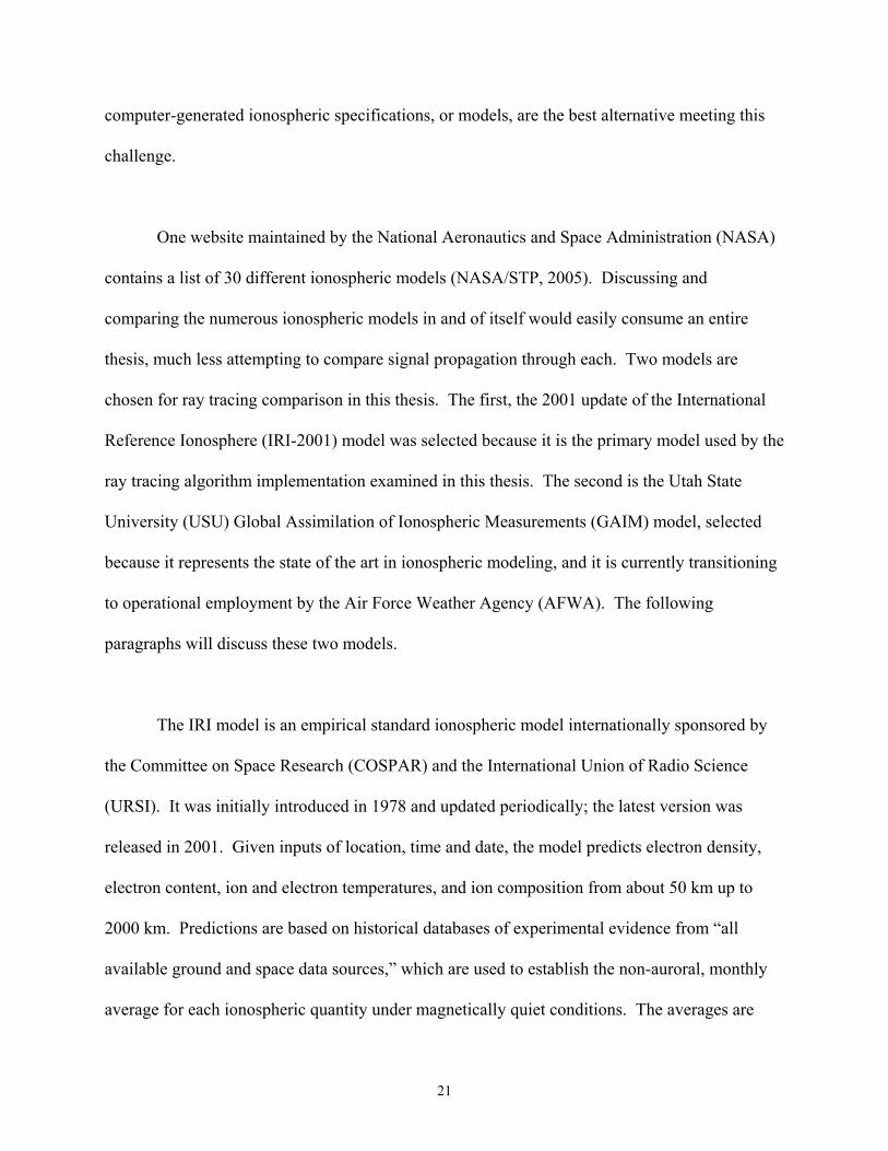
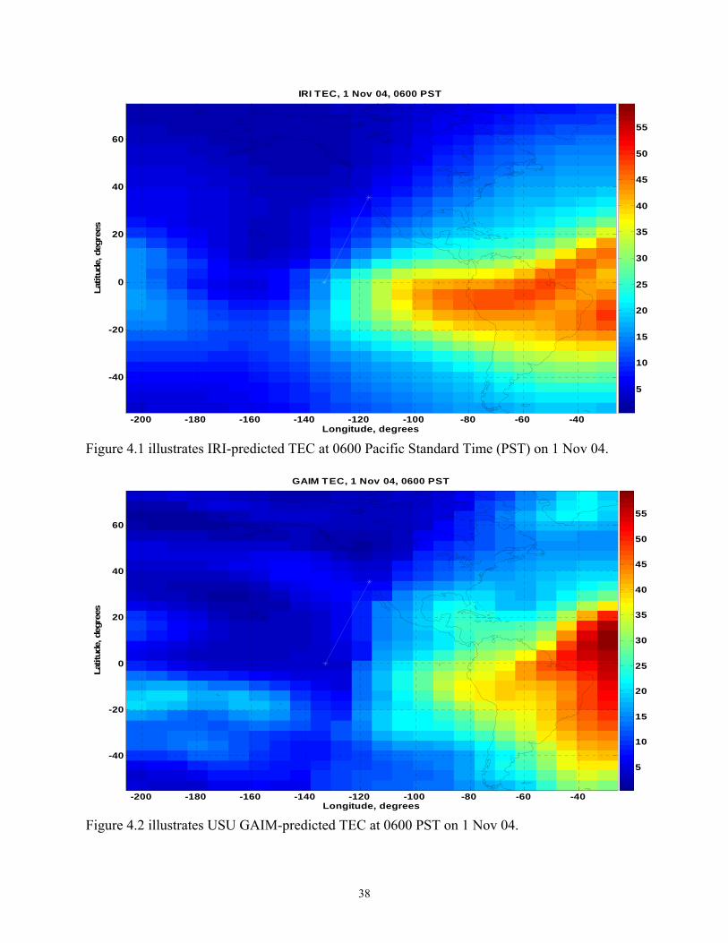
pproximate time the ionosphere’s peak density is expected over Goldstone. Figures 4.1 through
4.4 are TEC maps of IRI-2001 and USU GAIM specifications without the diffusive equilibrium
extension (DEE) model (TEC summed across altitudes 90 km to 1340 km). Figures 4.6 and 4.7
show TEC for DEE IRI and DEE GAIM, and figures 4.5 and 4.8 provide difference TEC maps
to help compare corresponding results. Each is discussed in the following paragraphs.
Iono
o
ble to expect the predicted TEC from these two models to be different because IRI mak
predictions based on historical average, magnetically-quiet ionospheric conditions, while GA
makes predictions based on actual conditions. These TEC (1 TEC = 1016 electrons per square
meter) maps are calculated from model plasma frequency specifications by first converting the
to electron density specifications, then obtaining the TEC within each latitude-longitude
(Lat/Lon) grid by finding the mean
m
for this thesis, Goldstone Deep Space Observatory (Goldstone), in southern California,
sists of 30 divisions between -52.8333 and 72.8333 degrees North Lat, and 24 division
2004 at 0600 Pacific Standard Time (PST), near sunrise at Goldstone; and at 1400 PST, the
a
36

Figures 4.1 and 4.2 show TEC values predicted by IRI-2001 and USU GAIM at 0600
cal Goldstone time (Pacific Standard Time, PST). The most immediately notable difference is
ever,
n
lo
the distribution of the electron content predicted by each model, illustrated by the varying colors
(dark blue corresponding to the minimum TEC and dark red to the maximum TEC). According
to IRI at this time, the densest region is already extending over South America, past its west
coast, and well into the Pacific Ocean, with two separate peaks of approximately 48 TEC
between 10 and -20 degrees Lat. GAIM predicts lesser densities over most of South America,
with the densest ionospheric region still off the east coast. GAIM predicts higher peak densities
than IRI, at nearly 60 TEC, north of the Equator, while IRI’s peaks are in the south. How
both models predict the peaks are within 20 degrees of the equatorial region as expected give
the Sun’s energy is directed just south of the equator at this time of year. Both models predict
higher densities to the east in the figures, as one would expect given the sun’s position over the
Earth. Neither model predicts high electron densities affecting the ground-satellite LOS, which
would suggest less frequency-dependent refraction will occur at this time. It is reasonable to
expect that as the sun progresses westward, the higher densities will enter the signal path
resulting in increased refraction. And, if the current trend holds, GAIM’s higher densities
suggest its model will result in more signal refraction and greater signal delay, at least to the
altitude these TEC maps include (1,340 km). The next figures show the progression of the
ionosphere into the peak time of day, 1400 PST, when the maximum densities are expected over
the ground site, affecting signal propagation.
37
Longitude, degrees
Lat
de, d
eee
sIRI TEC, 1 Nov 04, 0600 PST
itugr
-200 -180 -160 -140 -120 -100 -80 -60 -40
-40
-20
0
20
40
6050
55
5
10
15
20
25
30
35
40
45
Figure 4.1 illustrates IRI-predicted TEC at 0600 Pacific Standard Time (PST) on 1 Nov 04.
Longitude, degrees
Latit
ude
deg
re
GAIM TEC, 1 Nov 04, 0600 PST
,es
-200 -180 -160 -140 -120 -100 -80 -60 -40
-40
-20
0
20
40
60
5
10
15
20
25
30
35
40
45
50
55
Figure 4.2 illustrates USU GAIM-predicted TEC at 0600 PST on 1 Nov 04.
38

Figures 4.3 and 4.4 show TEC values predicted by IRI-2001 and USU GAIM 2.1 at 1400
PST. Similar to figures 4.1 and 4.2, the most immediately notable difference again is the
distribution of the ionospheric electron content predicted by each model. According to IRI at
this time, the densest region of more than 35 TEC, is well-spread on both sides of the Equator
between approximately -25 and 20 degrees Lon, and running the length of the figure. The two
peak-density regions predicted by IRI of over 50 TEC run nearly parallel, one peak close to the
equator and the other near the -20 degree Lat line. GAIM, on the other hand, predicts two much
more focused high density peaks up to nearly 70 TEC. The separation between the high density
regions is more defined in the GAIM result in which the differential between the highest peak
and the “valley” between the peak densities is approximately 25 TEC, whereas IRI’s peak-valley
differential is closer to 10 TEC. The densest regions predicted by GAIM also cover a smaller
approximately -20 to -180 degrees Lon, and sharply drop off above 20 Lat and below -26 Lat.
Common to model results is the appearance of density tails which stretch back to the
approximate location of the higher densities seen in the previous TEC plots at 0600. The
following map, figure 4.5, shows the TEC difference between the IRI and GAIM TEC maps at
1400. It is created by subtracting the GAIM TEC from the IRI TEC at each Lat-Lon grid point.
area of the map than IRI’s predictions, such that densities above 40 TEC extend from
39

Longitude, degrees
Latu
de,
gree
sIRI TEC, 1 Nov 04, 1400 PST
ti d
e
-200 -180 -160 -140 -120 -100 -80 -60 -40
-40
-20
0
20
40
60
10
20
30
40
50
60
Figure 4.3 illustrates IRI-predicted TEC at 1400 PST on 1 Nov 04.
Longitude, degrees
Latit
ude,
deg
rs
GAIM TEC, 1 Nov 04, 1400 PST
ee
-200 -180 -160 -140 -120 -100 -80 -60 -40
-40
-20
0
20
40
60
10
20
30
40
50
60
Figure 4.4 illustrates GAIM-predicted TEC at 1400 PST on 1 Nov 04.
40

Figure 4.5 assists in highlighting the major differences between the GAIM and IRI
predictions at 1400 PST. Overall, the magnitude of the average difference between the models is
just under 1 TEC at 0.91. However, the dark red indicates the regions where IRI predicts about
15 TEC more than GAIM, and the dark blue regions show GAIM at 20 TEC more than IRI.
These greatest differences correspond to different properties of each model’s TEC output.
Whereas GAIM’s peak differences clearly correlate to the peak TEC locations it predicts and the
tails stretching back across the map, IRI’s greatest differences correlate to its TEC
concentrations being spread over a larger area than GAIM. The final figures of this section will
explore if these differences translate to the DEE model specifications used for ray tracing.
Longitude, degrees
Latit
ude,
deg
rees
IRI - GAIM TEC Difference, 1 Nov 04, 1400 PST
-200 -180 -160 -140 -120 -100 -80 -60 -40
-40
-20
0
20
40
15
60
-20
-15
-10
-5
0
5
10
Figure 4.5 illustrates the predicted TEC difference between IRI and GAIM at 1400 PST on 1 Nov 04. This map is created by subtracting GAIM TEC from IRI TEC at every lat/lon grid point.
41

Figures 4.6 and 4.7 show TEC maps for DEE IRI and DEE GAIM at 1400 PST on 1
04, the same time as for figures 4.3-4.4. The difference plot in figure 4.8 of DEE IRI minus DEE
GAIM highlights the high DEE IRI bias in these results; the DEE IRI-predicted TEC map is
hundreds of TEC units greater than that of DEE GAIM. Although the magnitude of the
difference is surprising, this outcome is not completely unexpected considering the DEE IR
profile versus the DEE GAIM profile seen in chapter three, figure 3.4, shows IRI plasma
frequencies (proportional to electron densities) are significantly higher than GAIM’
models’ upper altitudes (at approximately 1380 km). Because the IRI-derived extension added
to GAIM is simply the portion of DEE IRI above 1380 km, scaled by the ratio of the upper
Nov
I
s in both
altitude plasma frequencies of GAIM versus IRI, and because IRI plasma frequency is
apparently greater than GAIM plasma frequency at 1380 km in figure 3.4, DEE IRI remains
greater than DEE GAIM above 1380 km for this single case. However, there is wide acceptance
in the ionospheric community that IRI’s topside ionospheric predictions for electron density are
higher than truth (Nickisch, 2006). Therefore, if USU GAIM’s upper altitude electron densities
are closer to truth than IRI’s, or if they are at least always less than IRI’s, it can be expected that
DEE IRI-predicted TEC maps will typically dominate the corresponding DEE GAIM-predicted
TEC maps. Moreover, given the basic relationships found in equations 2.1 through 2.5
explaining how signal refraction and group path rely on ionospheric electron density and TEC, if
large differences between DEE IRI and DEE GAIM TEC maps persist, there should be notable
differences in ray-tracing through these specifications. The next section compares some ray-
DEE IRI and DEE GAIM.
tracing refraction predictions based on un-extended IRI and GAIM specifications, and the last
two sections confirm there are significant differences in results based on ray tracing through
42

Longitude, degrees
Latu
de,
gree
sDEE IRI TEC, 1 Nov 04, 1400 PST
ti d
e
-200 -180 -160 -140 -120 -100 -80 -60 -40
-40
-20
0
20
40
60
50
100
150
200
250
300
350
400
Figure 4.6 illustrates diffusive equilibrium extended IRI at 1400 PST on 1 Nov 04.
Longitude, degrees
Latit
ude
deg
ree
DEE GAIM TEC, 1 Nov 04, 1400 PST
,s
-200 -180 -160 -140 -120 -100 -80 -60 -40
-40
-20
0
20
40
60
10
20
30
40
50
60
70
80
90
ive equilibrium extended GAIM at 1400 PST on 1 Nov 04. Figure 4.7 illustrates diffus
43

Longitude, degrees
Latit
ude,
deg
rees
DEE IRI - DEE GAIM TEC Difference, 1 Nov 04, 1400 PST
-200 -180 -160 -140 -120 -100 -80 -60 -40
-40
-20
0
20
40
60
50
100
150
200
250
300
350
Figure 4.8 illustrates the predicted TEC difference between diffusive equilibrium extended
ersions of IRI and GAIM at 1400 PST on 1 Nov 04. This map is created by subtracting GAIM TEC from IRI TEC at every lat/lon grid point. v
44

Ray Refraction
The following figures illustrate how ray tracing through un-extended IRI and GAIM
specifications predicts frequencies of 11, 12, 13, and 14 MHz will refract through the ionosphere
above Goldstone on 1 Nov 04, at 1400 PST. The results illustrated in figures 4.9 through 4.12
provide insight into how changing the transmitted signals’ elevation angles between 20, 45, and
70 degrees causes variation in the amount of refraction below 1,000 km altitude for each model.
One major difference found in figures 4.9 and 4.10, and important to applications such as OTHR,
HF, and DF is that a 12-MHz ray, launched at 45 degrees, penetrates the ionosphere predicted by
IRI but not by GAIM. The explanation, not well illustrated in these figures, is GAIM predicts a
higher electron density in the F2 region (at 250 km altitude) than IRI, resulting in the 12-MHz
e contained in a more compact layer (yellow-to-
yellow between approximately 200 and 350 km) than IRI (yellow-to-yellow at less than 200 up
to nearly 400 km). These differences in the peak densities and their distributions result in
differences in the predicted ray paths. GAIM shows more spread in the 45- and 70-degree rays
than IRI, but less spread in the 20-degree rays. Differences in ray spreading for each model are
also seen from directly above the ground site looking down at the ray paths projected onto the
Earth’s surface, herein called the “crossrange.” For instance, if the figures shown in figures 4.9
and 4.10 are in the x-z plane of the Cartesian coordinate system the crossrange view is looking
straight down the z-axis at the x-y plane. The crossrange results corresponding to figures 4.9 and
4.10 are shown in figures 4.11 and 4.12 and discussed next.
ray’s reflection. Another important difference is each model’s cross-sectional peak density
thickness. GAIM’s peak altitudinal densities ar
45

0 100 200 300 400 500 600 700 800 900 1000
1000
0
100
200
300
400
500
600
700
800
900
V (
icted Refraction, 11-14 MHz, 20-, 45-, and 70-deg, 1 Nov 04, 1400 PST
IRI-Preder
tical
km)
Dow nrange (km)
Figure 4.9 illustrates ray refraction for signals at 11, 12, 13, and 14 MHz, launched at 20, 45, and 70 degrees elevation through IRI-2001 at 1400 PST on 1 Nov 04.
0 100 200 300 400 500 600 700 800 900 1000
700
300
400
500
600
200
100
0
800
900
1000
Vical (k
Dow nrange (km)
GAIM-Predicted Refraction, 11-14 MHz, 20-, 45-, and 70-deg, 1 Nov 04, 1400 PST
Figure 4.10 illustrates ray refraction for signals at 11, 12, 13,
ert
m)
and 14 MHz, launched at 20, 45,
and 70 degrees elevation through USU GAIM at 1400 PST on 1 Nov 04.
46

Figures 4.11 and 4.12 correspond to figures 4.9 and 4.10, this time displaying crossrange
ray paths for signal frequencies of 11-14 MHz transmitted at angles of 20, 45, and 70 degrees
elevation. The rays diverge more quickly at higher transmission elevation angles. These figures
provide a key perspective on why a fully three-dimensional ray tracing algorithm is essential to
this research effort versus two-dimensional ray tracing methods, such as that discussed by
Coleman for OTHR (Coleman, 1998). Noting the difference in the figures y-axes’ scales, GAIM
predicts a 13-MHz ray launched at 45 degrees elevation diverges from the same signal launched
at 20 degrees elevation by more than 20 km crossrange in its first 1000 km of altitudinal
propagation, while IRI only predicts an approximately 8-km divergence for this signal. IRI
predicts a maximum divergence for the 12-MHz signal launched at 45 degrees of almost 12 km,
I does not clearly show any
initial negative crossrange tendency. Divergence is frequency dependent in both models,
wherein lower-frequency, non-reflected rays diverge more and high-frequency rays diverge less
for a given elevation angle. Of key interest to OTHR is the difference in IRI- versus GAIM-
predicted ray reflection. All frequencies are reflected for 20-degree elevation angles and both
models predict a tendency for all frequencies to propagate back towards zero crossrange, which
suggests a two-dimensional ray tracing algorithm would be sufficient. However, the 45-degree
elevation case shows no return to zero crossrange for the IRI 11-MHz and GAIM 11- and 12-
MHz reflections. The next section provides insight into the variation of transionospheric signal
elevation and azimuth angles as a function of frequency and time of day, which is of interest to
while GAIM predicts this signal is reflected. GAIM also predict all rays are initially being
refracted more towards the negative crossrange direction, while IR
applications such as OTHR, HF, DF, and SATCOMM.
47

0 200 400 600 800 1000 1200-2
12
0
2
4
6
8
10
Cro
ssr
ge (k
m
Dow nrange (km)
IRI-Predicted Crossrange Refraction, 11-14 MHz, 20-, 45-, and 70-deg, 1 Nov 04, 1400 PST
Figure 4.11 shows signal refraction projected on the Earth’s surface for 11, 12, 13, and 14 MHz, launched at 20, 45, and 70 degrees elevation through IRI-2001 at 1400 PST on 1 Nov 04.
an)
0 200 400 600 800 1000 1200
25
-5
0
5
10
15
20
Css
ran
(km
)
Dow nrange (k
GAIM-Predicted Crossrange Refraction, 11-14 MHz, 20-, 45-, and 70-deg, 1 Nov 04, 1400 PST
Figure 4.12 shows signal refraction projected on the Ear
roge
m)
th’s surface for 11, 12, 13, and 14 MHz, launched at 20, 45, and 70 degrees elevation through USU GAIM at 1400 PST on 1 Nov 04.
48

Angular Deviation
The LOS elevation and azimuth angles to a arbitrarily chosen satellite at geosynchronous
orbit (PanAmSat’s Galaxy 1R at 0°N Lat, 133°W Lon) from the Goldstone ground site in
southern California (35.424707°N Lat, 116.88982°W Lon) are different from the elevation and
azimuth at which the ground station antenna should be aimed to ensure the best signal reception
at frequencies below 1 GHz. The following ray-tracing results provide predictions for the best
signal elevation and azimuth transmission angles for transionospheric communications at
frequencies in this range. These angles result from ray tracing through DEE IRI and DEE GAIM
as a function of frequency, 15-50 MHz in steps of 5 MHz and 100-1000 MHz in steps of 100
penetrate the ionosphere as modeled by IRI and GAIM. The lower bound of 15 MHz is chosen
because this portion of the studied frequency range increases in increments of 5 MHz and
frequencies at or below approximately 11 MHz are already shown to be reflected by IRI and
GAIM. The times of this study are chosen somewhat arbitrarily with the intent to characterize
the majority of one ionospheric day. However, it should be noted that a full investigation would
incorporate multiple days, varying season, and solar cycle, and include nighttime studies as well.
This limited study begins with figures 4.13 and 4.14 illustrating elevation angular deviation from
LOS predicted by ray tracing through DEE IRI and DEE GAIM specifications.
MHz, and time of day, every 30 minutes between 0600 and 1700 PST, on 1 Nov 04. This
section specifically seeks to investigate the angular behavior of signals that consistently
49

6 7 8 9 10 11 12 13 14 15 16 17-2.5
-2
1
-1.5
-1
-0.5
0
0.5
Time of Day, Local Hours
ioat
ir
DEE IRI Ray-Tracing PredictionElevation versus T ime of Day and Frequency
15MHz20MHz25MHz30MHz35MHz40MHz45MHz50MHz100MHz
Elev
atn
Dev
ion
, deg
ees
200MHz300MHz400MHz500MHz600MHz700MHz800MHz900MHz1GHz
S for
signals from 15 MHz to 1 GHz, and every half hour from 0600 to 1700 PST on 1 Nov 04. Figure 4.13 illustrates DEE IRI ray-tracing-predicted deviation of elevation angle from LO
6 7 8 9 10 11 12 13 14 15 16 17-2.5
-2
-1.5
-1
-0.5
0
0.5
1
Time of Day, Local Hours
eve
d
DEE GAIM Ray-Tracing Prediction
Elat
ion
Dvi
atio
n,eg
rees
Elevation versus T ime of Day and Frequency
15MHz20MHz25MHz30MHz35MHz40MHz45MHz50MHz100MHz200MHz300MHz400MHz500MHz600MHz700MHz800MHz900MHz1GHz
Figure 4.14 illustrates DEE GAIM ray-tracing-predicted deviation of elevation angle from LOS for signals from 15 MHz to 1 GHz, and every half hour from 0600 to 1700 PST on 1 Nov 04.
50
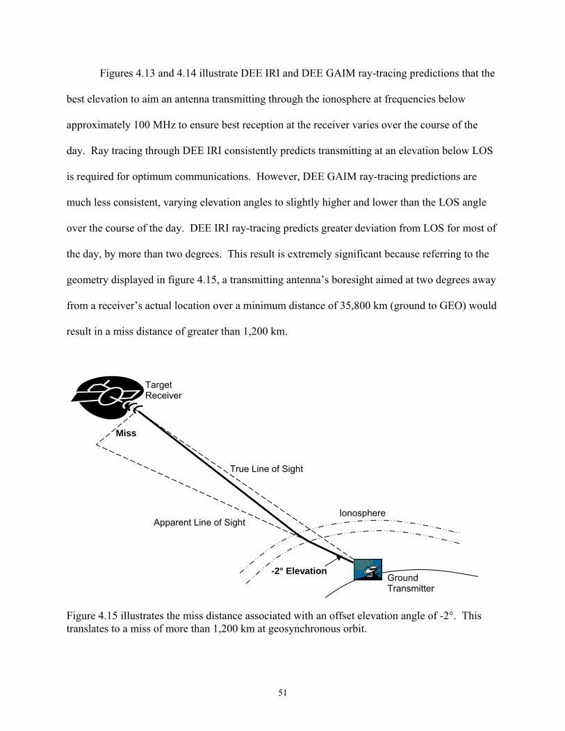
Figures 4.13 and 4.14 illustrate DEE IRI and DEE GAIM ray-tracing predictions that the
best elevation to aim an antenna transmitting through the ionosphere at frequencies below
approximately 100 MHz to ensure best reception at the receiver varies over the course of the
day. Ray tracing through DEE IRI consistently predicts transmitting at an elevation below LOS
is required for optimum communications. However, DEE GAIM ray-tracing predictions are
much less consistent, varying elevation angles to slightly higher and lower than the LOS angle
over the course of the day. DEE IRI ray-tracing predicts greater deviation from LOS for most of
the day, by more than two degrees. This result is extremely significant because referring to the
geometry displayed in figure 4.15, a transmitting antenna’s boresight aimed at two degrees away
from a receiver’s actual location over a minimum distance of 35,800 km (ground to GEO) would
Figure 4.15 illustrates the miss distance associated with an offset elevation angle of -2°. This
result in a miss distance of greater than 1,200 km.
translates to a miss of more than 1,200 km at geosynchronous orbit.
Ionosphere
Ground Transmitter
-2° Elevation
Miss
True Line of Sight
Apparent Line of Sight
Target Receiver
51

The objective of optimizing the transmitting antenna’s aim is to ensure the most efficient
communications by using the best signal path. If the transmitting antenna is aimed at the L
the satellite receiver, there is an associated miss distance similar to that shown in figure 4.15,
caused by ionospheric refraction. While DEE IRI ray tracing predicts as much as a two degree
adjustment, DEE GAIM results indicate much smaller elevation angle adjustments are necess
The DEE GAIM ray-tracing predictions also suggest that this adjustment will approach and pass
through the LOS elevation angle several times over the course of the day. Both results show that
as the frequency increases, the best transmission elevation collapses to the LOS, which agrees
with the expectation shown in figure 2.4 where increasing frequency signals are less refracted.
Also notable in the predictions from ray tracing through both DEE IRI and DEE GAIM, all
higher frequencies are contained under the “envelo
OS to
ary.
pe” of the lower frequencies, i.e. no higher
equency deviates more from the LOS than a lower frequency for any time of day. Moreover,
r
frequencies, and frequencies above approximately 100 MHz do not visibly deviate from the LOS
fr
frequencies above 100 MHz show no visible deviations from LOS during the period of interest.
A final difference between these apparent elevation angle predictions is there is no clear
correlation between the deviation predictions from ray tracing DEE IRI versus DEE GAIM. It
seems impossible to estimate the predictions of one given the predictions of the other. On the
other hand, the results shown in figures 4.16 and 4.17 displaying deviation of apparent azimuth
angles from LOS are much more similar.
Figures 4.16 and 4.17 show the DEE IRI and DEE GAIM ray-tracing predicted degree of
azimuth deviation from LOS as a function of frequency and time of day. As seen in the
elevation deviation results, higher frequencies are contained under the “envelopes” of the lowe
52

azimuth
after
s tends
ensate may cause signals transmitted from the ground
be refracted by the ionosphere to thousands of kilometers off target. The next section
. These results again concur with expectations of refraction as a function of frequency.
The DEE IRI result again predicts a maximum angular deviation for 15 MHz of approximately
negative two degrees from LOS. However, this is where the similarities between these results
and the previous elevations results end. The DEE GAIM result is much more similar to the DEE
IRI result. Before 1130 PST, DEE GAIM ray tracing predicts negative peak deviations from
LOS within one half hour and within 0.5 degrees of those predicted by ray tracing DEE IRI.
Both results predict a single zero deviation crossing of the LOS azimuth axis and both models
progress from negative to positive deviation in the afternoon. However, the DEE GAIM result
again appears jagged versus the DEE IRI result’s smooth progression during the day and DEE
GAIM’s result crosses the zero at 1330, while DEE IRI’s does so just before 1600. Further,
the zero crossing, DEE GAIM shows higher deviation than DEE IRI. Figure 4.18 helps clarify
why these zero crossing predictions occur. As the ionosphere’s peak electron density passes
from east to west with the sun’s progression, through the signal path, the best antenna azimuth
for optimal communications passes through the LOS azimuth, such that the antenna alway
to point into higher electron densities to compensate for ionospheric refraction of the signal to
the target receiver. In concluding this section, referring back to figure 4.15, it is clear that
compensating for transionospheric signal azimuth and elevation deviations is vital to improving
satellite communications. Failure to comp
to
provides another important consequence of the ionosphere’s impact on the signal path: varying
group path length.
53

6 7 8 9 10 11 12 13 14 15 16 17-2
-1.5
0
-1
-0.5
0.5
Time of Day, Local Hours
zim
uth,
egre
esDEE IRI Ray-Tracing Prediction
Azimuth versus Time of Day and Frequency
15MHz20MHz25MHz30MHz
A d 35MHz
40MHz45MHz50MHz100MHz200MHz300MHz400MHz500MHz600MHz700MHz800MHz900MHz1GHz
Figure 4.16 illustrates DEE IRI ray-tracing-predicted deviation of azimuth angle from LOS for signals from 15 MHz to 1 GHz, and every half hour from 0600 to 1700 PST on 1 Nov 04.
6 7 8 9 10 11 12 13 14 15 16 17-2
-1.5
-1
-0.5
0
0.5
Time of Day, Local Hours
mgr
Azimuth versus Time of Day and Frequency
Azi
uth,
de
ees
DEE GAIM Ray-Tracing Prediction
15MHz20MHz25MHz30MHz35MHz40MHz45MHz50MHz100MHz200MHz300MHz400MHz500MHz600MHz700MHz800MHz900MHz1GHz
Figure 4.17 illustrates DEE GAIM ray-tracing-predicted deviation of azimuth angle from LOS for signals from 15 MHz to 1 GHz, and every half hour from 0600 to 1700 PST on 1 Nov 04.
54

Figure 4.18 illustrates why the signal path azimuth deviation from LOS passes through the LOS azimuth (deviation passes through zero from negative to positive) as the ionospheric peak density (red) progresses from east to west over the course of the day. In order to maintain optimal communications between a transmitter and target receiver, the transmitter must aim into the higher density region to account for refraction of the signal.
transmitter
target
morninafternoonevenin
higher densit
higher densithigher
densit
North
Negative Azimuth Deviation
Zero Azimuth Deviation
Positive Azimuth Deviation
55

Signal Group Path
frequency and Goldstone local
time of day. Again, as seen in the angular deviation section, higher-frequency ray-tracing
predictions are contained within the envelopes provided by the lower frequencies. Frequencies
above approximately 100MHz again show almost no deviation from a minimum group path,
which is the LOS, or free space path distance between the Goldstone and the Galaxy 1R,
approximately equal to 37,394.029 km (determined by ray tracing through both models with a
frequency of 1000 GHz). The most notable differences include the deviation of the DEE IRI
ray-tracing-predicted ground path length from the LOS path length is typically on the order of
hundreds of kilometers higher than the DEE GAIM ray-tracing-predicted group paths for
The length of signal propagation paths between the Galaxy 1R satellite and Goldstone are
a function of the ionospheric index of refraction and TEC. The varying refractive index non-
uniformly alters the phase velocity of signals causing their associated EM wavefront or phase
group to change direction as it propagates through the medium. In effect, the signal phase group
travels longer paths and takes more time to propagate between the transmitter and receiver than
would be the case in free space, where the refractive index equals one. Additionally, equation
2.5 provides the approximate relationship between TEC and group path length. The difference
between the free space path length and the actual signal path length is critical to applications that
rely on signals to calculate distance to targets, such as various methods of DF and OTHR do for
target coordinate registration.
Figures 4.19 and 4.20 illustrate the signal group path lengths predicted by ray tracing
through DEE IRI and DEE GAIM respectively, as a function of
56

4
6 7 8 9 10 11 12 13 14 15 16 17
3.74
3.75
3.76
3.77
3.78
3.79
3.8x 10
Local Time of Day (hours)
Gro
upat
h (k
Pm
)DEE IRI Ionospheric Ray-Tracing Predicted
Group Path versus T ime of Day and Frequency
15MHz20MHz25MHz30MHz35MHz40MHz45MHz50MHz100MHz200MHz300MHz400MHz500MHz600MHz700MHz800MHz900MHz1GHz
ray-tracing-predicted group path length for signals from 15 MHz
0600 to 1700 PST on 1 Nov 04. Figure 4.19 illustrates DEE IRIto 1 GHz, and every half hour from
6 7 8 9 10 11 12 13 14 15 16 17
3.74
3.75
3.76
3.77
3.78
3.79
3.8x 10⁴
Local Time of Day (hours)
rh
(
DEE GAIM Ionospheric Ray-Tracing PredictedGroup Path versus T ime of Day and Frequency
Gou
p Pa
tkm
)
15MHz20MHz25MHz30MHz35MHz40MHz45MHz50MHz100MHz200MHz300MHz400MHz500MHz600MHz700MHz800MHz900MHz1GHz
15
MHz to 1 GHz, and every half hour from 0600 to 1700 PST on 1 Nov 04. Figure 4.20 illustrates DEE GAIM ray-tracing-predicted group path length for signals from
57

frequencies less than approximately 35MHz. Further, the DEE IRI result appears to have one
true maximum while the DEE GAIM result displays a dual-peak structure over the course of the
day. It is interesting to note that the peak group paths through each model arise hours before the
time peak electron densities are expected to be over the ground site (1400 Local). The predicted
peak group paths occur close to local noon. What makes this result even more unexpected is that
the LOS, shown in figures 4.1-4.8, points to the southwest from the ground site up through the
ionosphere. This would seem to suggest higher electron densities should not cause peak group
paths until sometime after the expected 1400 peak overhead electron density time. This odd
timing of peak group path lengths certainly demands future research, but is beyond the scope of
this thesis. The next chapter summarizes and concludes the findings of this thesis. It will
include suggested alternatives for future research to provide better insight into oddities such as
the timing of the peak group path.
58

V. Conclusion
Summary
The results of this thesis provided basic insights into the predictions of transionospheric
signal refraction and group paths obtained using ray-tracing theory interfacing with ionospheric
model specifications. Of the primary two models compared, IRI is a well-established,
climatological model considered by many in the international ionospheric community as the
standard of ionospheric models, and USU GAIM is a data assimilation model just recently
becoming operational through the Air Force Weather Agency for use by U.S. national defe
activities. The Hausman-Nickisch updated Jones-Stephenson Ray-Tracing Algorithm was used
to ray trace through un-extended IR
nse
I and GAIM ionospheric specifications, and to ray trace
through the same specifications extended to above geosynchronous orbits using Fridman’s
diffusive equilibrium ionospheric model. The results included the following outputs from the
two primary models and from ray tracing through the various ionospheric specifications:
1) Predicted total electron content ionospheric maps
2) Predictions of ionospheric signal refraction versus frequency versus signal launch angle
3) Predictions of ionospheric signal refraction leading to angular deviation from the line of sight
to a target versus frequency and time of day
4) Predictions of signal group path length versus frequency and time of day
59

This thesis included ray-tracing predictio c refraction and group delay effects on
gnals in the frequency range of 11 MHz to 1 GHz; the range in which applications such as
HF, and SATCOMM depend on transionospheric signals. The results contained
erein were intended to help users of applications such as the above to determine if ray-tracing
predict
further
hich
on
than a
w interesting questions for future research. Some of the questions raised and ideas for future
f this thesis: Future Research.
ns of ionospheri
si
OTHR, DF,
h
ions might assist them in reducing errors caused by ionospheric effects. Users may be
able to compare errors they are seeing in their applications to the results shown in this thesis or
they may wish to fund their own studies and provide “ground truth” data to compare to
ray-tracing predictions. These results might also help application users determine which
ionospheric model, IRI or GAIM, might be more appropriate to their needs depending on w
set of results more closely match any recorded signal angular deviations or path delays they are
able to compare against. Additionally, these results provide insight into the frequencies for
which there is a need to compensate for ionospheric refraction and path distortion; depending
the amount of error an application can tolerate, ionospheric affects on signals at frequencies
above approximately 100 MHz are much less significant than the effects seen in signals whose
frequencies are below 100 MHz. Finally, the results from this thesis certainly raise more
fe
research are discussed in the following, final section o
60

Future Research
Some of the more interesting results and areas recommended for further research inclu
1) Determining more accurate methods versus using a diffusive equilibrium model to extend
ionospheric specifications to GEO from lower altitude models such as IRI and GAIM in order
provide better ray-tracing predictions to assist in optimizing applications such as SATCOMM.
Appendix E discusses an attempt to extend GAIM specifications using an extrapolation method
2) A study on why the elevation angle ray-tracing predictions through DEE IRI were so
dissimilar from the predictions through DEE GAIM, while the azimuth predictions from the two
models were much more similar.
3) A comparison study of IRI, USU GAIM, and other models’ TEC map predictions (or othe
predictions from models) for a similar range of altitudes, which includes plots of the locations
and types of measurements included in the GAIM and other model specifications.
4) A study of ionospheric model ray-tracing predictions signal refraction and group path delays
over a longer period of time (days and nights), for varying season and/or solar cycle, or
comparing geomagnetic storm-time predictions versus non-storm-time results.
5) A study on why the group path distortions seen included peak distortion hours befo
de:
to
.
r
re the
expected time of peak ionospheric densities. This study could be accomplished beginning with
the relationship between signal group path length and the TEC in the signal group path given in
equation 2.5. The Hausman-Nickisch ray-tracing algorithm provides estimates of the signal path
TEC. A good thesis topic would be a comparison of ray-tracing signal path TEC predictions
versus TEC measured by GPS.
61

All of the future research ideas discussed here are graduate research opportunities and
ould be easily accomplished using the various process components already used in this thesis.
eric
g the
c
Continuing research in this area has the potential to provide highly valuable results to the
ionospheric community and to national defense activities. As the technology driving ionosph
modeling accuracy advances allowing for more accurate ray-tracing predictions of various
ionospheric signal effects, applications such as OTHR, HF, DF, and SATCOMM could benefit
by significant improvements to their operational accuracy. All that is needed is a voice to keep
the effort moving forward by highlighting the results being achieved and by demonstratin
future potential ray-tracing through ionospheric models holds for critical national defense
applications.
62

Appendix A: IRI Model Specification Input and Output Example
MakeIRITable.exe provided by L. J. Nickisch and Mark A. Hausman; example of inputs used for creating DiffusiveEquilibrium Extended (DEE) IRI specifications:
MakeIRITable.exe outputs a DEE IRI specification as a .TBL file that begins as follows, best viewed in Microsoft Wordpad: 221 nodes of altitudinal grid 80.000 81.000 82.000 … 36540.000 3 nodes of latitudinal grid -1.0000 0.0000 1.0000 3 nodes of longitudinal grid -1.0000 0.0000 1.0000 0.1707 0.1746 0.1779 … The last line shown here are the plasma frequencies (MHz) corresponding to the first altitude, first latitude, and first three longitudes specified (alt = 80.000; Lat = -1.0000; Lon = -1.0000, 0.0000, 1.0000). This DEE IRI specification continues with one plasma frequency output per altitude, latitude, and longitude, taking up hundreds of pages. USU GAIM 2.1 specifications of electron density are also hundreds of pages long, but are output in a very different format than this IRI .TBL file. A MATLAB m-file (GAIM4mat_xtend.m contained in Appendix B) was written to reformat the USU GAIM 2.1 specifications so they are in the same format (.TBL file and plasma frequencies) as the above DEE IRI specification, which is required for use by Nickisch-Hausman ray tracing algorithm. Additionally, the MATLAB file creates DEE GAIM specifications by combining the reformatted USU GAIM 2.1 specification with a scaled version of the high altitudes plasma frequencies from the DEE IRI specification for the same time, date, latitudes and longitudes.
63

Appendix B: MATLAB m-Files
%%%%%%%%%%%%%%%%%%%%%%%%%%%%%%%% % % Title: FullTECPlot.m % Description: Program to plot TEC maps from provided electron density % grids, and a TEC difference map for an IRI TEC map vs a GAIM TEC map. % Outputs: (file_name).TBL % Authors: Dr. Mark A. Hausman and Lt Shayne Aune % Organization/Office: AFIT/ENG % Last Updated: 18 Feb 06 % IMPORTANT NOTES: % (1) Requires another MATLAB script (I used a proprietary file % owned by NorthWest Research Associates) to read in electron density grids % (Negrids), altitudes, and latitudes and longitudes for the grid into % the MATLAB workspace prior to being able to plot any desired TEC maps. % (2) Requires geoshow toolbox for plots. % %%%%%%%%%%%%%%%%%%%%%%%%%%%%%%%%%%%%%%%%%%%%%%%%%%%%%%%% %%%%%%%%%%%%%%%%%%%%%%%%%%%%%%%%%%%%%%%%%%%%%%%%%%%%%%%% % Create first TEC grid % Find mean Ne between alt grid locations (cm^-3) Nemean1 = (Negrid1(2:end,:,:)+Negrid1(1:end-1,:,:))/2;
alt1 = (altgrid1(2:end)-altgrid1(1:end-1)); % altitude separation (km)
hape(TEC1,nlatgrid1,nlongrid1)./(10^12); ectrons/m^-2)
model density grid rid2(1:end-1,:,:))/2;
end-1)); rid2-1,nlatgrid2*nlongrid2);
ad coast
%%%%%%%%%%%%%%%%%%%%%%%% FullTECPlot.m %%%%%%%%%%%%%%%%%%%%% %%%%%%%%%%%%%%%%%%%%%%%%
dNemean1 = reshape(Nemean1,naltgrid1-1,nlatgrid1*nlongrid1); TEC1 = (Nemean1' * dalt1) * 1.e5; % 1.e5 converts km to cm
EC1 = resT% vertical in TEC units (10^16 el % Create second TEC grid % Repeat above process for second
,:)+NegNemean2 = (Negrid2(2:end,:dalt2 = (altgrid2(2:end)-altgrid2(1:
emean2 = reshape(Nemean2,naltgNTEC2 = (Nemean2' * dalt2) * 1.e5; TEC2 = reshape(TEC2,nlatgrid2,nlongrid2)./(10^12); %Plots % Difference TEC Map figure(1), imagesc(longrid1-360,latgrid1,(TEC1-TEC2)) colorbar hold on
rid on glo
64

geoshow(lat,long) xlabel('Longitude, degrees','FontSize',16,'FontWeight','bol ) ylabel('Latitude, degrees','FontSize',16,'FontWeight','bold'
gca,'FontSize',16,'FontWeight','bold')
layType','point','Marker','*','Color', 'w','MarkerSize',10) ,'Color', 'w','MarkerSize',10)
show(lat,long)
tle('Diffusive Equilibrium GAIM TEC, 1 Nov 04, 1400 PST','FontSize',16,'FontWeight','bold') t(gca,'FontSize',16,'FontWeight','bold')
pts=[-116.88982; -133.0];
,'Color','w','MarkerSize',10) eoshow(ypts(2),xpts(2),'DisplayType','point','Marker','*','Color','w','MarkerSize',10)
old on
ad coast
ld') Weight','bold')
,'FontWeight','bold') old')
pts=[-116.88982; -133.0]; pts=[35.424707; 0.0];
(ypts(1),xpts(1),'DisplayType','point','Marker','*','Color','w','MarkerSize',10) eoshow(ypts(2),xpts(2),'DisplayType','point','Marker','*','Color','w','MarkerSize',10)
','w')
%%%%%%%%%%%%%%%%%%%%%%%%%%%%%%%%%%%%%%%%%%%%%%%%%%% %%%%%%%%%%%%%%%%%%%%%%%%%%%%%%%%%%%%%%%%%%%%%%%%%%%
%%%%%%%%%%%%%%%%%%% End of FullTECPlot.m %%%%%%%%%%%%%%%%%%%%
d')
title({'Diffusive Equilibrium GAIM1 - GAIM2 TEC Difference'; '1 Nov 04, 1400 PST'},'FontSize',16,'FontWeight','bold') set(set(gca,'YDir','normal') xpts=[-116.88982; -133.0]; ypts=[35.424707; 0.0]; geoshow(ypts(1),xpts(1),'Dispgeoshow(ypts(2),xpts(2),'DisplayType','point','Marker','*'geoshow(ypts,xpts,'Color','w') % First model TEC map figure(2),imagesc(longrid1-360,latgrid1,TEC1) colorbar hold on grid on load coast geoxlabel('Longitude, degrees','FontSize',16,'FontWeight','bold') ylabel('Latitude, degrees','FontSize',16,'FontWeight','bold') tiseset(gca,'YDir','normal') xypts=[35.424707; 0.0]; geoshow(ypts(1),xpts(1),'DisplayType','point','Marker','*'ggeoshow(ypts,xpts,'Color','w') % Second model TEC map figure(3),imagesc(longrid1-360,latgrid1,TEC2) colorbar hgrid on logeoshow(lat,long) xlabel('Longitude, degrees','FontSize',16,'FontWeight','boylabel('Latitude, degrees','FontSize',16,'Fonttitle('Extrapolated GAIM TEC, 1 Nov 04, 1400 PST','FontSize',16set(gca,'FontSize',16,'FontWeight','bset(gca,'YDir','normal') xygeoshowggeoshow(ypts,xpts,'Color %%%%%%%%%%%%%%
65

%%%%%%%%%%%%%%%%%%%%%%% GAIM4mat_xtend.m %%%%%%%%%%%%%%%%%%%%% %%%%%%%%%%%%%%%%%%%%%%%%%%
ile, new_GAIM) %%%%%%%%%%%%%%%%
t GAIM netcdf file to .tbl file in format required ing IRI based diffusive equilibrium model
d IRI_file are the file paths and new_GAIM is the
da and Lt Shayne Aune Organization/Office: AFIT/ENG
6 a .nc file and MATLAB netCDF toolbox.
%%%%%%%%%%%%%%%%%%%%%%%%%%%%%%%%%%%%%%%%%%%%%%%%%%% %%%%%%%%%%%%%%%%%%%%%%%%%%%%%%%%%%%%%%%%%%%%%%%%%%%%
sion Diffusive Equilibrium data
in .TBL file
r i = 4088:999+1213:length(d),
indx+1;
AIM data using MATLAB netCDF toolbox etCDF file')
ens = den(:);
plsm = [];
%%%%%%%%%%%%%%%%%%%%%%%%%%%%%%function gaim_table = GAIM4mat_xtend(GAIM_file, IRI_f%%%%%%%%%%%%%%%%%%%%%%%%%%%%%%%%%%%%%%%%% % Title: GAIM4mat_xtend.m % Description: Reforma% for raytrace and extend us% Inputs: GAIM_file an% desired output file name % Outputs: (file_name).TBL % Authors: Lt Col Matthew Go%% Last Updated: 18 Feb 0% Notes: Requires GAIM ionospheric model as % %%%%%%%%% % Read in IRI extendisp('Read Diffusive Equilibrium Extension') % IRI_file = 'IRI3dLL_25Oct04-1400.TBL'; fid=fopen(IRI_file); d=fscanf(fid,'%c'); fclose(fid); % Set data for inclusionDE_alt=str2num(d(1251:2250)); indx = 1; DE_EC = zeros(720,100); fo EC=str2num(d(i:i+999)); DE_EC(indx,:)=EC; indx = end % Extract Gdisp('Read GAIM n% GAIM_file = 'GMF20042991400.NC'; gaim = netcdf(GAIM_file); alt = gaim{'Altitudes'}; lat = gaim{'Latitudes'}; lon = gaim{'Longitudes'};den = gaim{'Edensity'}; alts = alt(:); alt2 = [alts' DE_alt]; lats = lat(:); lons = lon(:); ddens = sqrt(dens).*8.9785282*10^-3; % Assemble GAIM into 2D matrix
66
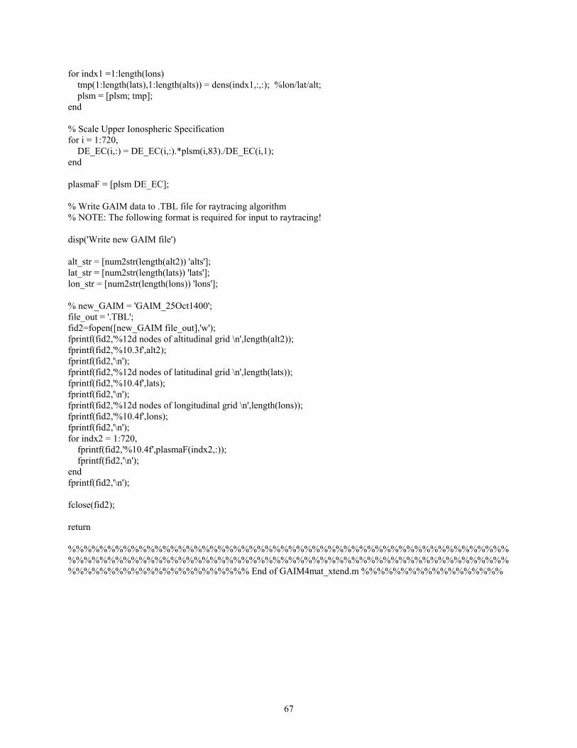
for indx1 =1:length(lons) tmp(1:length(lats),1:length(alts)) = dens(indx1,:,:); %lon/lat/alt; plsm = [plsm; tmp]; end % Scale Upper Ionospheric Specification
raytracing algorithm mat is required for input to raytracing!
('Write new GAIM file')
t_str = [num2str(length(lats)) 'lats'];
AIM file_out],'w'); %12d nodes of altitudinal grid \n',length(alt2));
rintf(fid2,'%10.3f',alt2);
inal grid \n',length(lats)); 2,'%10.4f',lats);
nal grid \n',length(lons));
intf(fid2,'%10.4f',plasmaF(indx2,:)); fprintf(fid2,'\n');
%%%%%%%%%%%%%%%%%%%%%%%%%%%%%%%%%%%%%%%%%%%% %%%%%%%%%%%%%%%%%%%%%%%%%%%%%%%%%%%%%%%%%%%%%%%%%
%%%%%%%%%%%% End of GAIM4mat_xtend.m %%%%%%%%%%%%%%%%%%
for i = 1:720, DE_EC(i,:) = DE_EC(i,:).*plsm(i,83)./DE_EC(i,1); end plasmaF = [plsm DE_EC]; % Write GAIM data to .TBL file for % NOTE: The following for disp alt_str = [num2str(length(alt2)) 'alts']; lalon_str = [num2str(length(lons)) 'lons']; % new_GAIM = 'GAIM_25Oct1400'; file_out = '.TBL'; fid2=fopen([new_Gfprintf(fid2,'fpfprintf(fid2,'\n'); fprintf(fid2,'%12d nodes of latitudfprintf(fidfprintf(fid2,'\n'); fprintf(fid2,'%12d nodes of longitudifprintf(fid2,'%10.4f',lons); fprintf(fid2,'\n'); for indx2 = 1:720, fpr end fprintf(fid2,'\n'); fclose(fid2); return %%%%%%%%%%%%%%%%%%%%%%%%%%%%%%
67

%%%%%%%%%%%%%%%%%%%%%% RayOutput.m %%%%%%%%%%%%%%%%%%%%%%%%%% %%%%%%%%%%%%%%%%%%%%%%%
tle: RayOutput.m Description: Program to get data from several raytracing .OUT files using the
sults. hayne Aune
te Last Updated: 18 Feb 06
%%%%%%%%%%%%%%%%%%%%%%%%%%%%%%%%%%%%%%%%%% %%%%%%%%%%%%%%%%%%%%%%%%%%%%%%%%%%%%%%%%%%%%%%%%%%%%%%%
ncatenated with file path in function RaytraceOut.m
_50.out'; _50.out';
leb(1,:) = 'IRI\Time_of_Day\1400_100_1000.out'; 0_1000.out';
ut(filea(i,:))]; aytraceOut(fileb(i,:))];
d Plots
e signal propagation in km/sec 9; % Range in km estimated by raytracing 1000 GHz signal
zi = -153.513186; % Azimuth in degrees estimated by raytracing 1000 GHz signal 650; % Elevation in degrees estimated by raytracing 1000 GHz signal
f Day Data imes = Data(1,:)-800;
Get Frequencies
for i = 1:2 GP(i,:) = Data(5,18*i-17:18*i); end % Calculate group delays Delays = (GP-TruRng)/c;
%%%%%%%%%%%%%%%%%%%%%%%%%%%%%%%%%% % Ti%% RaytraceOut function and plot desired re% Author: Lt S% Organization/Office: AFIT/ENG % Da%%%%%%%%%%%%%%%% clear; % Specify file path(s) to be co filea(1,:) = 'IRI\Time_of_Day\1400_15filea(2,:) = 'IRI\Time_of_Day\1430_15 fifileb(2,:) = 'IRI\Time_of_Day\1430_10 % Get data from files Data = []; for i = 1:2, Data = [Data RaytraceO Data = [Data Rend % Calculations an c = 299792.458; % Speed of free spacTruRng = 37394.02TruATruElev = 45.439 % Get Time oT %Freqs = Data(2,:); % Create Group Path Surface
68

% Plot 3D Delays versus Frequency versus Time of Day surf(Freqs,Times',Delays)
ours')
Signal Delays versus Time of Day and Frequency'})
%%%%%%%%%%%%%%%%%%%%% End of RayOutput.m %%%%%%%%%%%%%%%%%%%%%%
hold on grid on xlabel('Frequency, MHz') ylabel('Time of Day, Local Hzlabel('Delays, seconds') title({'IRI Predicted'; 'Ionospheric %%%%%%%%%%%%%%%%%%%%%%%%%%%%%%%%%%%%%%%%%%%%%%%%%%%%%%%% %%%%%%%%%%%%%%%%%%%%%%%%%%%%%%%%%%%%%%%%%%%%%%%%%%%%%%%% %
69

%%%%%%%%%%%%%%%%%%%%%% RaytraceOut.m %%%%%%%%%%%%%%%%%%%%%%%%% %%%%%%%%%%%%%%%%%%%%%%%%%%%%%%%%%%%%%%%%%%%%%%%%%%%%%%%
eOut(file_str) %%%%%%%%%%%%%%%%%%%%%%%%%%%%%%%%%%%%%%%%%%%%%%%%%%%
, azimuth, elevation, Group nd LOG TEC from ray tracing .OUT file.
Organization/Office: AFIT/ENG
% .OUT files. Additionally, it depends on the type of ray tracing being done, % i.e. this program may not work for non-homing ray trace output files. % %%%%%%%%%%%%%%%%%%%%%%%%%%%%%%%%%%%%%%%%%%%%%%%%%%%%%%%% %%%%%%%%%%%%%%%%%%%%%%%%%%%%%%%%%%%%%%%%%%%%%%%%%%%%%%%% disp('Read Raytrace Output File') % Open Output File path_dir = 'C:\WINDOWS\UnzipRaytrace\Results\'; %file_str = 'IRI\Baseline5\Baseline5_11_15.out'; fid=fopen([path_dir file_str]); % Read Data d = fscanf(fid,'%c'); fclose(fid); % Find and return Time, Frequency, Azimuth, Elevation, Group Path, Geometric Path indx = 1; tt = strfind(d,'@IRI3dLL_'); tim = str2num(d(tt+17:tt+21)); if tim<0200, tim = tim+2400; end k = strfind(d,'*** USING HOMER: RAY HOMING ALGORITHM ***'); k(end+1)=length(d); data_out = zeros(7,length(k)-1); for ii = 2:length(k) rng = k(ii-1):k(ii); d2 = d(rng); k2 = strfind(d2,'ITERATION'); klast = k2(length(k2)); d3 = d2(klast:end); frqf = strfind(d3,'FREQUENCY ='); freq = str2num(d3(frqf+12:frqf+18)); flg = strfind(d3,'PENETRATION FAILURE:');
%function data_out = Raytrac%%%%%% % Title: RaytraceOut.m % Description: Function to read time, frequency% Path, Geometric Path, a% Authors: Lt Col Matthew Goda and Lt Shayne Aune %% Last Updated: 22 Jan 06 % Note: This file specifically reads outputs from the Nickisch-Hausman % ray-tracing algorithm and is unlikely to be compatible with any other
70

bad = length(flg); % There is no output if penetration failure occurs flg2 = strfind(d3,'Off Grid'); bad2 = length(flg2); if(bad2)
az = str2num(d3(frqf+61:frqf+71));
pathf = strfind(d3,'RCVR'); 1:pathf+90));
gePath = str2num(d3(pathf+101:pathf+110)); num(d3(pathf+113:pathf+120));
z elev gpPath gePath LOGTEC]'; indx = indx+1;
turn %%%%%%%%%%%%%%
%%%%%%%%%%%%%%%%%%%%%%%%%%%%%%%%%%%%%%%%%%%%%%%%%%% %%%%%%%%%%%%%%%%%%%%% End of RaytraceOut.m %%%%%%%%%%%%%%%%%%%%%
disp('OFF GRID') end if (bad) az = NaN; elev = NaN; gpPath = inf; gePath = inf; LOGTEC = NaN; else elef = strfind(d3,'ELEVATION ANGLE OF TRANSMISSION ='); elev = str2num(d3(elef+35:elef+45)); gpPath = str2num(d3(pathf+8 LOGTEC = str2 end data_out(:,indx) = [tim freq a end re%%%%%%%%%%%%%%%%%%%%%%%%%%%%%%%%%%%%%%%%%%%%%%%%
71

72
Input and Output Examples
mple Input .DAT File for Nickisch-Hausman Ray Tracing Algorithm:
207.0 'DEG' / FINAL AZIMUTH ANGLE / STEP IN AZIMUTH ANGLE
GLE FINAL ELEVATION ANGLE
G' / STEP IN ELEVATION ANGLE
ver altitude (km) OF HOPS NUMBER OF STEPS PER HOP
89.9999 'DEG' / LATITUDE OF GEOMAGNETIC POLE (RAD) EOMAGNETIC POLE (RAD)
/ STOPRAY (use STOPCHK routine)
2. / PHASE PATH ! =1 TO INTEGRATE
2 1 / GENERATE PUNCHED OUTPUT FILE 81 5 / PLOT FLAG 83 -52. 'DEG' / LATITUDE OF BOTTOM EDGE OF PLOT 84 -205. 'DEG' / LONGITUDE OF LEFT EDGE OF PLOT 85 72. 'DEG' / LATITUDE OF TOP EDGE OF PLOT 86 -27. 'DEG' / LONGITUDE OF RIGHT EDGE OF PLOT 100 1 / READ TABLEX DATA 320 0. / POWER FLAG (1 = on, REQUIRED for ray homing) 321 1. / Do not use REACH 330 0.0 / Latitude for HOMING 331 -133. / Longitude for HOMING 332 0.001 / Accuracy // / End of input parameters !*********************************************************************** @IRI3dLL_01Nov04-2200.tbl / The .TBL model specification file used for trace !-----------------------------------------------------------------------
Appendix C: Nickisch-Hausman Ray Tracing Algorithm Exa 'AHWFNC' 'T3DLLLOG' 'NOELECT1' 'HARMONY' 'NOCOLFRZ' !----------------------------------------------------------------------- Homing Rays of a 11-14 MHz / Description of ray trace 1 1 / ORDINARY RAY 4 35.424707 'DEG' / NORTH GEOGRAPHIC LATITUDE OF TRANSMITTER 5 -116.88982 'DEG' / EAST GEOGRAPHIC LONGITUDE OF TRANSMITTER 7 11.0 / INITIAL FREQUENCY (MHZ) 8 14.0 / FINAL FREQUENCY (MHZ) 9 1.0 / STEP IN FREQUENCY (MHZ) 11 207.0 'DEG' / INITIAL AZIMUTH ANGLE 12 13 0. 'DEG' 15 15. 'DEG' / INITIAL ELEVATION AN16 15. 'DEG' / 17 0. 'DE19 0. / 3=HOMER one freq, 7=HOMER multiple freq 20 35800. / Recei22 1 / NUMBER
1.E4 / MAXIMUM23 24 25 0.00 'DEG' / LONGITUDE OF G26 1 / Number of ground reflections 29 1 30 50000. / Stop at group path of 50000 km 42 1.E-9 / MAXIMUM RELATIVE SINGLE STEP ERROR 45 100. / MAXIMUM INTEGRATION STEP LENGTH (KM) 57 60 2. / PATH LENGTH ! =2 TO INTEGRATE AND PRINT 62 2. / TEC 63 1. / TEC**2 1 0 / NUMBER OF STEPS BETWEEN PERIODIC PRINTOUTS 77

Example Outpu C:\WINDOWS\Un 'AHW !--- Rays 1 4 5 'D 7 8 9 11 'D 12 'D 13 15 16 17 19 20 22 23 24 25 26 un 29 TO 30 pa 42 VE 45 AT 57 60 62 63 71 S 72 ED 81 83 'DEG' TT 84 'DEG' EF 85 'DEG' P
100 1 / READ TABLEX DATA 320 0. / POWER FLAG (1 to turn on - REQUIRED for 321 / do not use REACH 330 331 332 01 // !********************************************************************* @IRI v04-2200. * 221 nodes of altitudinal grid * 80.000 81.000 82.000 83.000 84.000 85.000 86.000
t .O
zipR
FNC'---- of -1 2 2
35 50
-
-
3dLL
UT
ay
'--a 35161114 10707 1 1 80 8 00 10 -520 7
13
_0
Fi
tra
T3D---var1 .42.88.0 .0 .0 .0 .0 0. 5. 5. 0. 0. 0. 1 1.9.0.1 1 0. 1.0. 2. 2. 2. 1. 0 1 5 2. 5. 2.
1. 0.03. 0.0
1No
le
E4 99900
E-9
fro
ce\f
LLLO----ying
4707 982
9
m
or
G'-- f
Ni
t.
'--re
'D
' ' ' ' ' '
cki
9
NOE---que
DDEGDEGDEG
DEGDEG
sc
LE--nc
EG' EG'
EG' EG' EG'
' ' ' ' '
/ / /
tbl
h-H
CT--y
au
1' --
/ / / / / / / / / / / / / / / / / / / / / / / / /
/ / / / / / / /
86 -27. 'DEG' / LONGITUDE OF RIGHT EDGE OF PLOT
sm
'--
ORNOEAINFISTINFISTINFIST3=reNUMALALOn
STStMAMAPHPATETENUGEPLLALOLA
an
HAR---
DINRTHST ITINALEP ITINALEP ITINALEP HOMceiMBEXIMTITNGIumbOPRop XIMXIMASETH C C**MBENEROT TITNGITIT
R
MO--
AR GGEAL FINAL AINAL EINERveR UMUDTUerAYat UM UM PLE 2 R ATFLUDTUUD
ay
NY--
Y EOOG FRE F AZI A ELE E ar OF NE DE o (
Tr
' --
RAGRARAPREQQUREQZIMMUTZILEVALEt alH
UMOF O
f us
groRELINT
ATH NGTH OF SE PUAG E OF DE OE OF
aci
'NO---
Y
ENC
MVATTIOVATonetitOPSBERGE
F Ggroe Sup ATIEGR TEPNCH
BOF LTO
ng
CO--
PHICHIC UENC
Y UENCUTH H ANUTH
ION IO fud OOMEO
A
LF--
LLOY (MY ANGLANN ANN ree
F
lgo
RZ--
ATNG(MHZ(MGLE GLANGLANq, (k
STAGNEMAGNd rePCHK th oSIN
ION BETWOUT
OM ET EDEDGE
rit
' ---
ITUITUHZ)) HZ)E
E GLEE GLE7=
m)
EPSTICETIflero
f 5GLESTE ! ! ! !EENPUT
DGEGE OF
hm
--
DEDE
HO
P PC ctut00 SP P F
OOF P
:
--
O O
ME
EROLPOioin0 TELE=1=2
ERIL
F PLO
--
F F
R
HE LE ns e) km P NG T T
IOE
PLLOT
---
TRATRA
at
OP (RA(R
ERRTH O IO I
DIC
OT T
--
mu
D)AD
OR(KNTNT
P
--
NSMINSMI
lt
()
M)EGEG
RI
--
TTTT
ip
us
RARA
NT
--
ER ER
l
e
TE TE
OUTS
73

* 30 nodes of latitudinal grid * -52.8333 -48.5000 -44.1666 -39.8333 -35.5000 -31.1666 -26.8333 * 24 nodes of longitudinal grid
02/07/ 6 MULA ORDINARY NO COLLISIONS
INTED
* 157.7500 165.2500 172.7500 180.2500 187.7500 195.2500 202.7500 0.2383 0.2618 0.3086 0.3975 * 0.2156 0.2211 0.2271
File too long to echo every line... !--------------------------------------------------------------------- 1Rays of a varying frequency launched at approximately 45 degrees
APPLETON-HARTREE FOR T3DLLLOG NOELECT1 HARMONY NOCOLFRZ INITIAL VALUES FOR THE W ARRAY -- ALL ANGLES IN RADIANS, ONLY NONZERO VALUES PR 1 1.00000000000E+00 2 6.37120000000E+03 4 6.18277773704E-01 5 -2.04011222106E+00 7 1.10000000000E+01 8 1.40000000000E+01 9 1.00000000000E+00 11 3.61283155163E+00 12 3.61283155163E+00 15 2.61799387799E-01 16 2.61799387799E-01 20 1.00000000000E+03 22 1.00000000000E+00 23 1.00000000000E+04 24 1.57079458147E+00 26 1.00000000000E+00 29 1.00000000000E+00 30 5.00000000000E+04 41 3.00000000000E+00 42 1.00000000000E-09 43 5.00000000000E+01 44 1.00000000000E+00 45 1.00000000000E+02 46 1.00000000000E-08 47 5.00000000000E-01 48 1.00000000000E+02 57 2.00000000000E+00 60 2.00000000000E+00 62 2.00000000000E+00 63 1.00000000000E+00 71 1.00000000000E+04 72 -1.00000000000E+00 81 5.00000000000E+00
21 83 -9.07571 1037E-01 84 -3.57792496659E+00 85 1.25663706144E+00 86 -4.71238898038E-01 100 1.00000000000E+00 321 1.00000000000E+00 331 -1.33000000000E+02 332 1.00000000000E-03 Beginning one-time computation of SJ coefficients
74

75
5 6 G G N N
0.000000 0.000000 0.000000 0.000000
00091 0.000000 00393 0.000607
1 2 3 4 5 6 H H H H H N N N N N N
000000 0.000000 0.000000 0.000000 0.000000 0.000000 051861 0.000000 0.000000 0.000000 0.000000 0.000000 042983 0.003966 0.000000 0.000000 0.000000 0.000000 006969 -0.005682 0.003882 0.000000 0.000000 0.000000 015086 0.009075 -0.002506 0.002247 0.000000 0.000000 004453 -0.013211 0.006264 0.000872 -0.000746 0.000000 003289 -0.009519 -0.006486 0.003340 -0.000016 -0.000294 ncy launched at approximately 45 degrees 02/07/ 6 Y NOCOLFRZ APPLETON-HARTREE FORMULA ORDINARY NO COLLISIONS
CY = 11.000000 MHZ, AZIMUTH ANGLE OF TRANSMISSION = 207.000000 DEG ELEVATION ANGLE OF TRANSMISSION = 15.000000 DEG
AZIMUTH DEVIATION ELEVATION RANGE XMTR LOCAL XMTR LOCAL POLARIZATION GROUP PATH PHAS PATH GEOM PATH LOG TEC KM DEG DEG DEG DEG REAL IMAG KM KM KM CM-2 00 0.0000 15.000 0.000 -0.951 0.000 0.000 0.000 -10.000
Finished computation of SJ coefficients 1 0 1 2 3 4
G G G G G N N N N N
0.000000 0.000000 0.000000 0.000000 0.000000 0.296194 0.017282 0.000000 0.000000 0.000000 0.034016 -0.053146 -0.014470 0.000000 0.000000 0.000000 0.000000 -0.033490 0.070055 -0.024247 -0.005649 0.000000 0.000000 0.000000 -0.040788 -0.043541 -0.009783 0.008429 -0.000823 0.000000 0.000000
0.017231 -0.035725 -0.017084 0.006137 0.003740 0.0 -0.010438 -0.012892 -0.011089 0.016030 0.000322 -0.0
0 H H N 0.000000 0. 0.000000 -0. 0.000000 0. 0.000000 0. 0.000000 -0. 0.000000 -0. 0.000000 0.1Rays of a varying freque T3DLLLOG NOELECT1 HARMON FREQUEN HEIGHT KM -2.E-16 XMTR 0.00
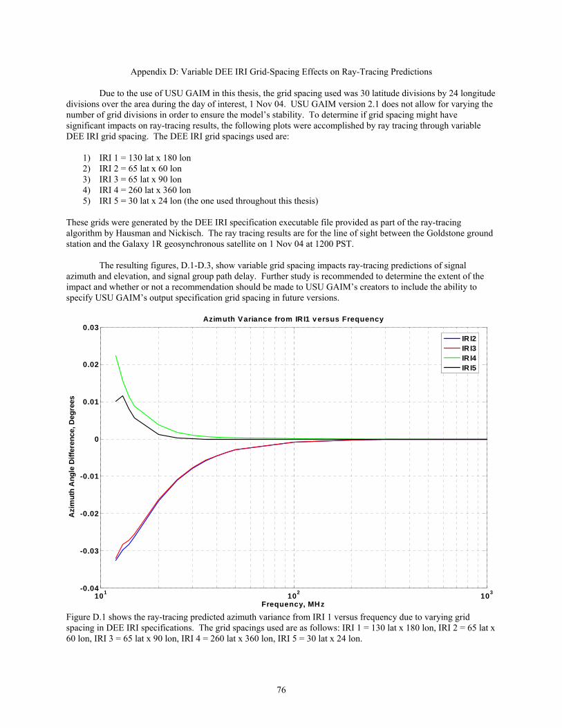
76
Appendix D: Variable DEE IRI Grid-Spacing Effects on R ng Predictions
Due to the use of USU GAIM in this thesis, the grid spacing used was 30 latitude divisions by 24 longitude divisions over the area during the day of interest, 1 Nov 04. USU GAIM 2.1 does not allow for varying the number of grid divisions in order to ensure the model’s stability. To de f grid spacing might have significant impacts on ray-tracing results, the following plots were acco by ray tracing through variable DEE IRI grid spacing. The DEE IRI grid spacings used are:
1) IRI 1 = 130 lat x 180 lon 2) IRI 2 = 65 lat x 60 lon 3) I lon
I 60 l is thesis)
T b ecutable file d as part of the ray-tracing al N ts he ight between the Goldstone ground s e v t 1200
e sp mp tracing predictions of signal a si r is rec ed to determine the extent of the im r de U Gs ut ut sion
a e requency due to varying grid
cat ar = 130 lat x 180 lon, IRI 2 = 65 lat x o I
ay-Traci
sione i
hed
videof s.
ray-end’s creators to include the ability to
us fI 1
lon.
vtermp
p lin P
acomAs.
ves: 2
erminlis
roe
ST
ts m
IM
rs IR4
RIRIRI
s by t
hendd w
U
s DI 3
3 4 5
we Hhe
r elh G
hoEE =
===
rea
G
esevetA
w
6
65 26 30
gusal
ultatheIM
s tIR5
l0 la
enmaax
inior o
’
heI slat
at lat
erny
g n,r s o
rpe x
x 90t x 3x 24
ated and1R g
figur andnot autp
ay-trcifi
90 l
4)
hego
tati
zimp
pec
iguac
0 l
lon on
y icos
s, Dgnec sp
cinio
n,
5
serion
uacif
rein
on
) I
gridthm and
Tth at any US
D.1g in, IR
(t
thekisyn
.alomec
g nsIR
he o
DEch. chro
1-D. grou
meifica
pred. ThI 4 =
ne
E Tno
3,p
ndtio
ice 2
u
IRheu
sh patn
tedgr60
sed
I ras s
owathion g
aid l
t
spy tate
d s
rid
zi spat
hr
ecrll
vaelho s
ma
x
ou
ifiaciite
riaayu
pa
uthcin36
gh
cang o
b. ldci
vg0
o
tio rn
le Fu beng
ars ulon
ut th
n exesul1 No
gridrthe ma in f
iancsed, IR
are for t 04 a
acing istudy to Uur
froe a5 =
Se ver
m Is fo 30
Fsp6
RIllo la
1wt x
101 102 103-0.04
-0.03
-0.02
-0.01
0
0.01
0.02
0.03
Fr
ce
equ
fro
en
Diff
eren
ce, D
egre
es
m ers encyAzimuth Varian
cy
IR
, MH
I1 v us Frequ
IRI2IRI3IRI4IRI5
Azi
mut
h A
ngle
z

E le v a tio n V a r ia n c e fro m IR I1 v e rs u s F re q u e n c y0 .0 6
Figure D.2 shows the ray-tracing predicted elevation variance from IRI 1 versus frequency due to varying grid spacing in DEE IRI specifications. The grid spacings used are as follows: IRI 1 = 130 lat x 180 lon, IRI 2 = 65 lat x 60 lon, IRI 3 = 65 lat x 90 lon, IRI 4 = 260 lat x 360 lon, IRI 5 = 30 lat x 24 lon.
rid Figure D.3 shows the ray-tracing predicted group delay variance from IRI 1 versus frequency due to varying g
spacing in DEE IRI specifications. The grid spacings used are as follows: IRI 1 = 130 lat x 180 lon, IRI 2 = 65 lat x 60 lon, IRI 3 = 65 lat x 90 lon, IRI 4 = 260 lat x 360 lon, IRI 5 = 30 lat x 24 lon.
1 0 1 1 0 2 1 0 3-6
-5
-4
-3
-2
-1
0
1
F r e q u e n c y , M H z
Gro
up D
elay
, mic
rose
cond
s
G r o u p D e la y V a r ia n c e f r o m IR I1 v s F r e q u e n c y
IR I2IR I3IR I4IR I5
1 0 1 1 0 2 1 0 3-0 .0 8
-0 .0 6
-0 .0 4
-0 .0 2
0
0 .0 2
0 .0 4
IR I2IR I3IR I4IR I5
ees
F re q u e n c y , M H z
Ang
le D
iffer
ence
, Deg
rEl
evat
ion
77

Appendix E: Attempted USU GAIM Model Specification Extrapolation
Figure E.1 illustrates an alternate attempt to provide USU GAIM ionospheric specifications up to geosynchronous orbits versus the diffusive equilibrium model extension method used in this thesis (resulting in DEE GAIM). Essentially, this extrapolation method intended to extrapolate GAIM specifications using a linear fit of the logarithm of the electron densities at GAIM highest three altitudes for each latitude-longitude grid point. It was assumed that the electron densities would be decreasing exponentially at the high altitudes of GAIM. However, the resulting extrapolated GAIM specifications were thrown out as an alternative due to results such as that shown in figure E.1, in which one of GAIM’s grid points had a positive slope for its highest three altitudes resulting in a logarithmically increasing electron density with altitude. This leads to in an inordinately high relative TEC value for the corresponding grid location. Note that the grid points close to the specific “bad” grid location have a similar tendency, although not as “bad,” and one of the affected grid points appears in the signal path. Therefore ray-tracing predictions along this path could be subject to the inaccuracies of the extrapolated specification. All of the ionospheric experts consulted for this research agreed this method was not appropriate for use in this thesis.
Extrapolated GAIM TEC, 1 Nov 04, 0600 PST
Longitude, degrees
Latit
ude,
deg
rees
-200 -180 -160 -140 -120 -100 -80 -60 -40
-40
-20
0
20
40
60
20
40
60
80
100
120
140
Figure E.1 illustrates extrapolated GAIM at 0600 PST on 1 Nov 04.
78

Bibliography
Bilitza, Dieter. International Reference Ionosphere 1990. National Space Science Data Center / World Data Center
A for Rockets and Satellites. Lanham: Science Applications Research, 1990. Bilitza, Dieter K. “International Reference Ionosphere 2000.” Radio Science, Vol. 36, Num 2 (2001): 261-275. Bilitza, Dieter K. “International Reference Ionosphere.” International Reference Ionosphere. 2005. National
Aeronautics and Space Administration, Goddard Space Flight Center, National Space Science Data Center. 14 Feb 2006 http://modelweb.gsfc.nasa.gov/ionos/iri.html.
Bilitza, Dieter K. Various e-mails to author. NASA/GSFC, NSSDC. 2006. Borer, William S. Presentations, personal interview, and by various e-mails to author. Air Force Research Lab Space
Vehicles Directorate. 2005-2006.
Budden, K. G. Radio Waves in the Ionosphere; the Mathematical Theory of the Reflection of Radio Waves from
Stratified Ionised Layers. Cambridge: Cambridge UP, 1961. CIRES, Webpage: http://cires.colorado.edu/science/projects/aoms-andersonD03.html. 2004. Coleman, C. J. “A Ray Tracing Formulation and its Application to Some Problems in Over-The-Horizon RADAR.”
Radio Science. Vol. 33, Num 4 (1994): 1187-1197. Hamilton, W.R. Third Supplement to treatise on geometrical optics. 1931. Hausman, Mark A. Various e-mails to author. NorthWest Research Associates. 2005-2006. Haselgrove, Jenifer. “Ray Theory and a New Method for Ray Tracing.” Report of Conference on the Physics of the
Ionosphere. London: London Physical Society, 355-364, 1954. Haselgrove, C. B., and Jenifer Haselgrove. “Twisted Ray Paths in the Ionosphere.” The University, Manchester.
Proc. Phys. Soc. London, Vol. 75, 357-361, 1960. Jones, R. Michael, and Judith J. Stephenson. A Versatile Three-Dimensional Ray Tracing Computer
Program for Radio Waves in the Ionosphere. Institute for Telecommunication Sciences, Office of Telecommunications, US Dept. of Commerce. Springfield: National Technical Information Service, 1975.
79

Keyser, Herbert L. VacDonnell, M. D. “A Fast Three-Dimensional Ray Tracing Formulation, with Applications to HF Communications
laide,
rious e-mails to author. Air Force Weather Agency. 2006. M
and RADAR Prediction.” 27 Apr. 2000. Dept. of Electrical and Electronic Eng., The Univ. of AdeSouth Australia. 14 Feb. 2006 http://www.ips.gov.au/IPSHosted/NCRS/wars/wars2000/commg/mcdonnell.pdf.
Misra. Global Positioning System, Signals, Measurements, and Performance. Lincoln: Ganga-Jamuna P, 2001. 137-138. NASA, Ionospheric Modeling Webpage: http://modelweb.gsfc.nasa.gov/models_home.html. 2006. NASA/JPL/California Institute of Technology, Deep Space Network Webpage: http://deepspace.jpl.nasa.gov/dsn/.
2006. NGDC/STP. Webpage: http://www.ngdc.noaa.gov/stp/IONO/grams.html. 2006. NetCDF Toolbox, MATLAB®, Webpage: http://mexcdf.sourceforge.net/netcdf_toolbox.html. 2006. Nickisch, L. J. “Focusing in the Stationary Phase Approximation.” Radio Science. Vol. 23, Num 2 (1988): 171-182. Nickisch, L. J. Various e-mails to author. NorthWest Research Associates. 2005-2006. Schunk, Robert W., and Andrew F. Nagy. Ionospheres, Physics, Plasma Physics, and Chemistry. New York:
Cambridge UP, 2000. 25-31. Schunk, Robert W., L. Scherliess, J. J. Sojka, and Don C. Thompson. Global Assimilation of Ionospheric
Measurements (GAIM): An Operational Space Weather Model. Second Symposium on Space Weather, 11 Jan. 2005, American Meteorological Society (AMS). 14 Feb 2006 http://ams.confex.com/ams/Annual2005/techprogram/paper_86412.htm.
Tascione, Thomas F. Introduction to the Space Environment. 2nd Ed. Malabar: Krieger Company, 1994. 113-114. Thompson, Don C. Various e-mails to author. Utah State University Center for Atmospheric and Space Sciences.
2006.
User’s Guide Version 2.1, Global Assimilation of Ionospheric Measurements model. 2004.
80

Vita
Clarksville, Tennessee;
owever, as a youth he attended schools across the country and abroad as part of a military family. He completed
ndergraduate studies at Virginia Polytechnic Institute and State University (Virginia Tech) and graduated with a
’s
Educatio 5, AFROTC at Virginia Tech. He received
e Society of American Military Engineer’s Outstanding Senior ROTC Engineering Student award, and he was
cognized as the AFROTC Blue Chip recipient, third in his class.
st
tour was Foreign Language Center at the Presidio of Monterey, California, with
llow-on training at Goodfellow AFB in San Angelo, Texas, to complete initial career training as a Spanish
Cryptolo
enter (MRSOC) on Kelly AFB in San Antonia, Texas, initially assigned to the 93rd Intelligence Squadron. In
996, he was selected for promotion to senior airman below-the-zone and moved to the 543 Intelligence Group
lectronic Intelligence (ELINT) career field, from which he graduated as the Top Graduate. He was then assigned
rformed routine duties maintaining the
onstant Web intelligence database, while also serving as a squad leader on the Air Intelligence Agency’s all-
olunteer Honor Guard. In 1998, he completed Airman Leadership School receiving the John L. Levitow award for
san AB, Republic of South Korea, where he performed duties as a Foreign Instrumentation Signals Intelligence
is unit’s NCO of the Year for 2000. In May 2004, he entered the Air Force Institute of Technology (AFIT). At
ificate in
Measure
ffice.
Second Lieutenant Shayne C. Aune graduated from Northwest High School in
h
u
Bachelor of Science degree in Electrical Engineering in May 2004. He was commissioned through the Airman
n and Commission Program (AECP) through Detachment 87
th
re
Lieutenant Aune has had an extensive Air Force career since his enlistment in December 1993. His fir
to the Defense Language Institute-
fo
gic Linguist. His second tour was to the Medina Regional Signals Intelligence (SIGINT) Operations
C
rd1
Commander’s office as a protocol specialist. He returned to Goodfellow AFB in 1997 for cross-training into the
E
to the Air Force Information Warfare Center (AFIWC), Kelly AFB, and pe
C
v
leadership. He was then selected as the AFIWC Junior Enlisted Member of the Year for 1998. His next tour was to
O
(FISINT) analyst. There he was selected for AECP, promoted to SSgt, selected for promotion to TSgt, and named
h
AFIT he finished the online Basic Acquisitions Officer course (ACQ101) and received a graduate cert
ments and Signatures Intelligence (MASINT). His follow-on assignment is to the National Reconnaissance
O
81

Form Approved REPORT DOCUMENTATION PAGE OMB No. 074-0188
The public reporting burden for this collection of information is estimated to average 1 hour per response, including the time for reviewing instructions, searching existing data sources, gathering and maintaining the data needed, and completing and reviewing the collection of information. Send comments regarding this burden estimate or any other aspect of the collection of information, including suggestions for reducing this burden to Department of Defense, Washington Headquarters Services, Directorate for Information Operations and Reports (0704-0188), 1215 Jefferson Davis Highway, Suite 1204, Arlington, VA 22202-4302. Respondents should be aware that notwithstanding any other provision of law, no person shall be subject to an penalty for failing to comply with a collection of information if it does not display a currently valid OMB control number. PLEASE DO NOT RETURN YOUR FORM TO THE ABOVE ADDRESS. 1. REPORT DATE (DD-MM-YYYY) 23-03-2006
2. REPORT TYPE Master’s Thesis
3. DATES COVERED (From – To) Aug 04 – Mar 06
5a. CONTRACT NUMBER
5b. GRANT NUMBER
4. TITLE AND SUBTITLE Comparison of Ray Tracing through Ionospheric Models 5c. PROGRAM ELEMENT NUMBER
5d. PROJECT NUMBER
5e. TASK NUMBER
6. AUTHOR(S) Aune, Shayne C., 2d Lt, USAF
5f. WORK UNIT NUMBER
7. PERFORMING ORGANIZATION NAMES(S) AND ADDRESS(S) Air Force Institute of Technology
8. PERFORMING ORGANIZATION REPORT NUMBER Graduate School of Engineering and Management (AFIT/EN)
2950 Hobson Way WPAFB OH 45433-7765
AFIT/GE/ENG/06-04
10. SPONSOR/MONITOR’S ACRONYM(S)
9. SPONSORING/MONITORING AGENCY NAME(S) AND ADDRESS(ES) AFRL/VSBXP NRO/SIGINT/GSO Attn: Dr. William Borer, GS-15 Attn: James Bolles, Lt Col, USAF 29 Randolph RD 14675 Lee Road Hanscom AFB, MA 01731 Chantilly, VA 20151-1715 DSN: 478-3039 Comm: 703-808-2681
11. SPONSOR/MONITOR’S REPORT NUMBER(S)
12. DISTRIBUTION/AVAILABILITY STATEMENT APPROVED FOR PUBLIC RELEASE; DISTRIBUTION UNLIMITED.
13. SUPPLEMENTARY NOTES
14. ABSTRACT A comparison of ray tracing predictions for transionospheric electromagnetic wave refraction and group delays through ionospheric models is presented. Impacted applications include over-the-horizon RADAR, high frequency communications, direction finding, and satellite communications. The ionospheric models used are version 2.1 of Utah State University's Global Assimilation of Ionospheric Measurements (USU GAIM) model and the 2001 version of the International Reference Ionosphere (IRI) model. In order to provide ray tracing results applicable to satellite communications for satellites at geosynchronous orbit (GEO), a third ionospheric model is used to extend the sub-2000-km USU GAIM and IRI ionospheric specifications to 36540 km in altitude. The third model is based on an assumption of diffusive equilibrium for ion species above 2000 km. The ray-tracing code used is an updated implementation of the Jones-Stephenson ray tracing algorithm provided by L. J. Nickisch and Mark A. Hausman. Ray tracing predictions of signal refraction and group delay are given for paths between Goldstone Deep Space Observatory near Barstow, California, and the PanAmSat Galaxy 1R satellite. Results are given for varying frequency between 11MHz to 1GHz, varying time of day between 0600 and 1700 Pacific Standard Time on 1 November 2004, and varying signal transmission elevation angle. Ray tracing predicts minimal ionospheric effects on signals at or above approximately 100 MHz. Signals below 100 MHz are predicted to refract on different paths by each model. Ray tracing in diffusive equilibrium extended (DEE) specifications of USU GAIM predicts as much as 500 km less group delay than in DEE IRI. This appears to be due to the diffusive equilibrium extension from typically higher electron densities predicted in the upper altitudes of IRI’s specifications. USU GAIM also indicates higher frequencies will not penetrate the ionosphere’s F2 region versus IRI-2001 during the period of interest. 15. SUBJECT TERMS ray tracing, raytracing, ionospheric models, Global Assimilation of Ionospheric Measurements model, USU GAIM, GAIM, International Reference Ionosphere model, IRI, ionospheric ray tracing, ionospheric raytracing
16. SECURITY CLASSIFICATION OF:
Standard Form 298 (Rev: 8-98) Prescribed by ANSI Std. Z39-18
19a. NAME OF RESPONSIBLE PERSON Matthew E. Goda, Lt Col, USAF
REPORT
U ABSTRACT
U c. THIS PAGE
U
17. LIMITATION OF ABSTRACT UU
18. NUMBER OF PAGES 19b. TELEPHONE NUMBER (Include area code) 94 (937) 255-3636 ext 4614; e-mail: