COMPARISON OF PLATE MODELS FOR ANALYSIS OF LAMINATED ...home.iitk.ac.in/~mohite/ictacem04.pdf ·...

COMPARISON OF PLATE MODELS FOR ANALYSIS OF LAMINATED COMPOSITES

P. M. Mohite and C. S. Upadhyay**

Department of Aerospace Engineering, IIT Kanpur 208016, INDIA, e-mail: [email protected] Assistant Professor, Department of Aerospace Engineering, IIT Kanpur 208016, INDIA e-mail:

[email protected]

ABSTRACT In the present study a family of plate models available for the analysis of laminated structures is compared for the point-wise data like transverse deflection and local state of stress. Here, the plate models compared are Higher-order-Shear-Deformable (HSDT) model, Hierarchic model and Layerwise model. It is seen that all the models predict the deflections accurately. The local state of stress is computed using direct finite element data and equilibrium approach of post processing as well. It is seen for HSDT and hierarchic models that the state of stress computed using direct finite element data is significantly different from exact one, whereas for the layerwise model it is accurately predicted. With equilibrium approach of post processing the local state of stress is accurately predicted by all the models. Further, the effect on first-ply failure load using Tsai-Wu failure criterion by these approaches for the extraction of stresses is studies. Further, the effect of discretisation error control by one shot adaptive approach developed by authors have been studied for the first-ply failure loads. It is seen that the control of discretisation error together with equilibrium approach of post processing leads to significant reduction in failure loads. NOTATION x, y, z Global coordinates u(x,y,z) General displacement field pxy In-plane approximation order pz Transverse approximation order a,b Plate dimensions t Thickness of laminate S Aspect ratio q0 Intensity of transverse loading INTRODUCTION Thin structures made of composite laminates are increasingly used in the manufacture of structural components. The enhanced strength to weight ratio makes composites especially attractive for aerospace applications. There is always demand to maximize the payload. All the problems posed in this context are constrained approximation problems with constraints on maximum transverse deflection, buckling load, failure load, natural frequency etc. It is imperative to estimate the constraint quantities accurately for an acceptable optimal design.

Onset of laminate failure is an important aspect for a designer. Onset of failure in composite laminated plates requires the local stress state to be known in the structure, particularly near structural details; at interlamina interface and in the individual lamina. Accurate prediction of the local stress state becomes important for a reliable estimate of the failure load, which may be crucial for a safe design of the component.

Several plate theories have been proposed in the literature (see Reddy ,1984-Ahmed and Basu 1994). The goal is generally to give a higher order representation of the

transverse shear terms, as in (Reddy, 1984) or to design families of plate theories with guaranteed convergence to the three-dimensional solutions in some norm (see Szabó et al. 1988-Actis et al. 1999). However, not much can be said about the accuracy of the local stress state and displacements. In the third type of plate models the individual lamina have continuous through thickness representation of displacements (see Ahmed and Basu, 1994). The goal of this study is to determine the quality of the local state of stress, obtained using various families of plate models commonly used in engineering practice. A detailed comparison will be done with respect to the exact three-dimensional elasticity solutions given in [Pagano and Hatfield, 1971-Pagano, 1970]. for both symmetric and anti-symmetric stacking of the laminae. The values of the in-plane stresses obtained directly from the finite element computations will be compared to the three-dimensional elasticity solution. The effect of model order and in-plane approximation order, on the accuracy of these stresses will be demonstrated. For the transverse stress components, the values obtained from the finite element solution directly, and those obtained using the equilibrium approach of post-processing, will be compared to the exact ones. Further, the study aims at clearly demonstrating the need for proper mesh design in the computation of critical failure loads. Another important goal of this study is to obtain reliable values of the first-ply failure load, using the available models, and compare them with those given in (Reddy and Reddy, 1992). It will be demonstrated that depending on the applied boundary conditions, stacking sequence and ply orientation, the reliable values of the first-ply failure load can be significantly lower than those obtained using the commonly used meshes and polynomial approximations. PLATE MODELS The system of partial differential equations of three dimensional elasticity is generally intractable analytically, especially for a layered medium. The development of classical theories was motivated to alleviate these problems by reducing the dimension for analysis. For example, in case of plates and shells reduction from three to two dimension reduces the computational cost and enables the handling of a large class of problems. Traditionally, for the plate and shell like thin structures, several plate theories have been proposed. These can be broadly classified as:

(1) Shear deformable theories (HSDT); (2) Hierarchic plate theories and (3) Layerwise theories

Shear Deformable Theory Here, one such theory due to (Reddy, 1984) is taken as representative theory from this group. It is a third order shear deformable theory. And imposes the condition of parabolic distribution of transverse shear strains through thickness of of the plate to satisfy the zero transverse shear stress on the top and bottom face of the plate. Hierarchic Plate Theory In these, the displacement components have a zig-zag or hierarchic representation through the thickness. The hierarchic plate models are a sequence of mathematical

models, the exact solutions of which constitute a converging sequence of functions in the norm or norms appropriate for the formulation and objectives of analysis. The construction of hierarchic models for homogeneous isotropic plates and shells was given by Szabó and Sharmann, 1988 and later for laminated plates by Babuška et al., 1992 and Actis et al., 1999. The solutions of the lower order models are embedded in the highest order model and these models can be adapted according to the requirement.

In these models the displacement field is given as product of functions that depend upon the variables associated with the plate, shell middle surface, and functions of the transverse variable. The transverse functions are derived on the basis of the degree to which the equilibrium equations of three-dimensional elasticity are satisfied. Layerwise Theory In these theories, the individual lamina has continuous through thickness representation of displacements. In the present study, the layer-by layer model proposed by Ahmed and Basu, 1994 is adapted. In this model, all the displacement components are represented as product of in-plane functions of same order and out-of-plane approximating functions of different order for ( )),vu and w . MATHEMATICAL FORMULATION OF PLATE MODELS The generic representation of the displacement field for the plate models is given as:

( )[ ] ( )yxzzyxwzyxvzyxu

zyx ,U),,(),,(),,(

),,u( φ=⎪⎭

⎪⎬

⎫

⎪⎩

⎪⎨

⎧= (1)

where

( )[ ]( ) ( ) ( )

( ) ( ) ( )( ) ( ) ⎥

⎥⎥

⎦

⎤

⎢⎢⎢

⎣

⎡=

L

L

L

zzzzz

zzzz

85

742

631

0000000000000000

φφφφφ

φφφφ (2)

and

( ){ } ( ) ( ) ( ) ( ) ( ){ }TyxUyxUyxUyxUyxUyxU ,,,,,, 84321 L= (3)

Note that ( ) ( ) ( )LyxUyxUyxU ,,,,, 631 , ……are the in-plane components of displacement terms ),,( zyxu . Similarly, ( ) ( ) ( )LyxUyxUyxU ,,,,, 742 are the in-plane components of displacement terms ),,( zyxv . The in-plane components of transverse displacement ),,( zyxw are given by ( ) ( )LyxUyxU ,,, 85 .The transverse functions are given in terms of the normalized transverse coordinate ztz )/2(ˆ = (where t is the thickness of the laminate). For the higher order shear deformable model the functions ( )zφ are given as:

( ) ( ) ( ) ,1521 === zzz φφφ ( ) ( ) ,43 zzz == φφ

( ) ( ) ( ) ( ) ,011876 ==== zzzz φφφφ ( ) ( ) 3109 zzz == φφ

Remark: The in-plane displacement components have cubic representation and transverse component is constant in laminate thickness. The quadratic term of in-plane displacement components drop out when the zero shear condition on the top and bottom face of the plate is enforced. For the hierarchic family of the plate models the transverse functions ( )zφ are given as:

{ } { } { };

)ˆ()ˆ();ˆ()ˆ();ˆ()ˆ(

)()ˆ()(;)()ˆ()ˆ(;)()ˆ()ˆ(

;ˆ)ˆ()ˆ(;)ˆ()ˆ()ˆ(

z4t

zz4t

zz4t

z

0-z2t

z0-z2t

z0-z2t

z2t

zzz1zzz

2

2

113

2

103

2

9

118227226

43521

ρφψφφφ

ρρφψψφϕϕφ

φφφφφ

===

===

=====

where

∫∫∫ −−−===

zzzzd

Qzzd

QQQQQ

zzdQQQ

QQz

ˆ

1 131

ˆ

1 2455544

45552

ˆ

1 2455544

45442 ˆ1)ˆ(;ˆ

--

)ˆ(;ˆ-

-)ˆ( ρψϕ

Where Qij are the coefficients of the global constitutive relation, in the global xyz -coordinate system. For other transverse functions see Actis et al., 1999.

The present layerwise plate model is an improvement over the model given In Ahmed and Basu, 1994, as the original layerwise model had same order transverse representation for all three displacement components, whereas the present layerwise model can have different approximation in transverse direction for individual displacement components. The different approximation for displacement components is used as suggested by Schwab, 1996, for a single lamina, to take into account the bending and membrane actions. The displacement component lu , for a prismatic element (i.e. triangular in-plane projection) in the thl layer, is given as

∑ ∑++

=

+

=)2)(1(

1

1

)(),(),,(xyxy

uzpp

j

p

k

lk

ljjk

l zMyxNuzyxu

where xyp and u

zp are the in-plane and transverse approximation order (for component lu ) and ( )yxN j , and ( )yxM k , are in-plane and transverse approximation functions,

respectively. Similarly the other components lv and lw can be expressed. The transverse approximation orders for u and v displacement components will be the same, while that for the component w can be different. Hierarchic basis functions will be used for in-plane and transverse representations of the solution components. The transverse

approximation functions are shown in fig. 1. In this study, 2=xyp or 3; uzp , 1=v

zp , 2, 3;

,0=wzp 1, 2, 3 will be used.

FINITE ELEMENT FORMULATION For a given lth lamina, the constitutive relationship in principal material directions is given as: { } [ ]{ })l()l()l( C ε=σ (4) where { }Tllllll

l)(

12)(

13)(

23)(

33)(

22)(

11)( σσσσσσσ = are the stress components for the layer, and

{ } { }Tlllllll

)(12

)(13

)(23

)(33

)(22

)(11)( γγγεεεε = are the components of strain. The subscripts 1, 2

and 3 denotes the three principal material directions. The constitutive relationship in global xyz coordinates can be obtained by usual transformations. The potential energy, Π, for the laminate is given by

{ }{ } ∫∫ −+=Π

RRdswqdv

U-

21

Vεσ (5)

Where V is the volume enclosed by the plate domain, R+ and R- are the top and bottom faces of plate and q(x,y) is the transverse applied load. The solution to this problem uex is the minimizer of the potential energy Π.

Fig. 1 Transverse approximation functions for single lamina in layerwise model

ERROR ESTIMATOR FOR LOCAL QUANTITY OF INTEREST In the analysis of laminates for first-ply failure the accurate computation of state of stress at a point is essential. When the finite element analysis is employed, the issue of control of modeling error (error due to model employed in the analysis of laminate, as compared to three dimensional elasticity) and discretization error becomes important. Adaptive methods for the control of discretization error are available in literature (see Verfürth, 1996). These are based on the control of energy norm of the error, ( )eue 2|||| =Ω (where

∪(e) is the strain energy norm of the error). This does not guarantee that the pointwise quantity of interest is also accurate. Various smoothening based a-posteriori error estimation techniques for laminated composites have been proposed by the authors for the local quantity of interest (see Mohite and Upadhyay, 2002). Further, estimation and control of the error in the quantity of interest and “one shot” adaptive approach for the control of discretization error was proposed in (Mohite and Upadhyay, 2003). Further, this approach is used for accurate computation of critical local quantities in (Mohite and Upadhyay, 2004). In the present study the issue of adaptive control of modeling error will not be addressed. The procedure given in (Mohite and Upadhyay, 2003) is used here. The quantity of interest is the stress component, which contributes maximum to the Tsai-Wu first ply failure index (Tsai and Wu, 1971). TSAI-WU FAILURE CRITERION It is a complete polynomial criterion and is an extension of the criterion used for anisotropic materials (see Tsai and Wu, 1971). The Tsai-Wu criterion is given by

1≥+= jiijiiTW FFFI σσσ (6) where iji FF , are the strength tensor terms and iσ are the stress components. NUMERICAL RESULTS One of the major goals of this paper is to do a critical analysis of various families of plate models, with respect to the quality of the point-wise stresses obtained using the models. The effect of in-plane approximation order, model order and type will also be investigated here. All the models are subjected to rigorous numerical studies to compare the transverse deflection and stress profiles for numerous ply orientations, stacking sequences and boundary conditions under transverse loadings. In the present study, three types of transverse loadings are considered, namely, uniform pressure, sinusoidal and cylindrical bending.

The numerical results are arranged in two sections. In the first section, the effect of the plate models on the accuracy of point-wise data, i.e. transverse deflection and all the stress components at a point, is addressed. The stress components are either computed directly using the constitutive equations, or the equilibrium equations are used to obtain the transverse normal and shear stresses. In the second section, the effect of the analysis models on the accuracy of first-ply failure load is addressed. Effect of Model on Accuracy of Point-wise Data Comparison of Transverse Deflections The goal of this numerical experiment is to compare the value of transverse displacement components obtained using various models, and in-plane discretization, with the exact three-dimensional elasticity results reported in (Pagano and Hatfield, 1972), for cross-ply laminate sequence with material properties given in table 1. The plate has dimension a along x -axis and b along y -axis, and is subjected to sinusoidal loading of the form ( ) ( ) ⎟

⎠⎞

⎜⎝⎛

⎟⎠⎞

⎜⎝⎛=

by

axyxqyxq ππ sinsin,, 0 (7)

All edges of the plate are simply supported (see table 2 for all BC’s used). The transverse deflection at ⎟

⎠⎞

⎜⎝⎛ 0,

2,

2ba is reported in tables 3 and 4. Note that in all the computations the

layerwise model uses (3,3,2) model (unless specified), that is, transverse approximation for u and v is cubic and quadratic for w . For the hierarchic family 11 field model is used, while for the HSDT model (3,3,0) approximation is used. Table 1 Material Properties for (Pagano, 1972-Pagano, 1970). Property E1 E2 G12 G23 υ 12=υ 23

Value 25×106 psi 106 psi 0.5×106 psi 0.2×106 psi 0.25 Table 2 Boundary conditions

Boundary Condition At y=0 and y=b At x=0 and x=a Soft Simple Support v=w=0 u=w=0

Clamped u=v=w=0 u=v=w=0 Free u, v, w≠0 u, v, w≠0

In this study following case has been studied: Square plate with cross ply laminae, such that outer laminae with orientation o0 and total thickness of o0 laminae is equal to total thickness of o90 laminae. Also laminae with

same orientation have equal thickness. In this study, 7 and 9 layered laminate is used. The

transverse deflection is nondimensionalised as tSq

Qww 40

4*

12π

= , where

( )[ ] ( )211223221112 1/214 ννν −+++= EEGQ . Here, 3=xyp is used for all models. Numbers in parenthesis show the % error with respect to exact solution.

Table 3:Non-dimensional transverse deflection ( )*w for 7 layered cross-ply laminate.

S Exact [12] Layer-wise HSDT Hierarchic 2 12.342 12.341 (0.00) 10.918 (11.54) 10.358 (16.07) 4 4.153 4.153 (0.00) 3.594 (13.46) 3.575 (13.92) 10 1.529 1.529 (0.00) 1.417 (7.33) 1.444 (5.56) 20 1.133 1.133 (0.00) 1.096 (3.26) 1.113 (1.76) 50 1.021 1.021 (0.00) 1.005 (1.56) 1.017 (0.39) 100 1.005 1.005 (0.00) 0.993 (1.19) 1.004 (0.09)

From these tables we observe that:

1. The layerwise model predicts the transverse deflection accurately for all the aspect ratios.

2. The HSDT and hierarchic model are far from the exact one for the aspect ratios upto 10=S . The error for this aspect ratios ranges from 5-16 %.

3. For the HSDT and hierarchic model with aspect ratios 10>S the displacement is close to exact. The error is 0.1-3 %.

Table 4:Non-dimensional transverse deflection ( )*w for 9 layered cross-ply laminate.

S Exact [12] Layer-wise HSDT Hierarchic 2 12.288 12.306 (-0.15) 10.703 (12.89) 11.632 (5.34) 4 4.079 4.079 (0.00) 3.530 (13.46) 3.664 (10.17) 10 1.512 1.512 (0.00) 1.406 (7.01) 1.438 (4.89) 20 1.129 1.129 (0.00) 1.093 (3.18) 1.110 (1.68) 50 1.021 1.020 (0.09) 1.001 (1.96) 1.017 (0.39) 100 1.005 1.005 (0.00) 1.004 (0.09) 0.993 (1.19)

Comparison of Stresses Here, various stress components for symmetric and antisymmetric laminates, under cylindrical bending, are compared with the exact values given in (Pagano,1972-Pagano, 1970). Case 1: In this case [0/90/0], square laminate with all edges simple supported is considered. All the laminae are of equal thickness. The sinusoidal loading is of the form as in above subsection. The in-plane stresses are nondimensionalised as

( ) ( )⎟⎟⎠

⎞⎜⎜⎝

⎛⎟⎠⎞

⎜⎝⎛= zzba

Sq xyxxxyxx ,0,0,,2

,2

1, 20

τστσ and the transverse stresses as

( ) ⎟⎟⎠

⎞⎜⎜⎝

⎛⎟⎠⎞

⎜⎝⎛= zb

Sq xzxz ,2

,01

0ττ . The in-plane stress components are shown in fig. 2 and transverse

stress component is shown in fig. 3. Case 2: In this case, [165/-165] laminate under cylindrical loading is considered. The loading is of the form ( ) ⎟

⎠⎞

⎜⎝⎛=

axqyxq πsin, 0 . The plate is infinite along y -direction. All the

laminae are of equal thickness. The stress components are nondimensionalised as

Fig. 2 [0/90/0] laminate; all edges simply supported, in-plane stresses.

Fig. 3 [0/90/0] laminate; all edges simply supported, transverse stresses. Equilibrium stressesDirect stresses

( ) ⎟⎟⎠

⎞⎜⎜⎝

⎛⎟⎠⎞

⎜⎝⎛

⎟⎠⎞

⎜⎝⎛= zaza

Sq xyxxxyxx ,2

,,2

1, 20

τστσ and ( ) ( ) ( )( )zzSq yzxzyzxz ,0,,01,

0ττττ = . The in-plane

stress components are shown in fig. 4 and transverse stress components are shown in fig. 5.

Fig. 4 [165/-165] laminate under cylindrical bending, in-plane stresses.

Direct stresses

Equilibrium stressesFig. 5 [165/-165] laminate under cylindrical bending, transverse stresses.

Case 3: The problem description is same as previous sub-subsection. The stress components are nondimensionalised as case 1 above. The point-wise stress values are given for layerwise model in tables 5 and 6. In these tables the first row gives the value at

0=z while in the second maximum values and in the third row their location quoted in parenthesis is reported for the components xzτ and yzτ . From the results it is observed that:

1. The in-plane stress components are accurately predicted by all higher order models.

2. The transverse shear stress components computed directly from finite element solution is accurate for the layerwise model whereas, those obtained by HSDT and hierarchic models are significantly different both qualitatively and quantitatively.

3. Using the equilibrium approach of post-processing leads to more accurate transverse stress components for all the models.

The layerwise model predicts accurately the point-wise values of the stress components for all the values of S . Effect of Models on Accuracy of Predicted Failure Load The laminates considered are [0/90]S and [-45/45/-45/45]. The plate is either clamped on all edges or simple supported. The top face of the plate is subjected to uniform transverse load ( ) 0, qyxq = . The plate dimensions are )9(9.228 inmma = and )5(127 inmmb = . The material properties are given in table 7. The first-ply failure load is nondimensionalised as 4

22

0 SEq

FLD = . The results obtained from the present analysis are compared with those

reported in (Reddy and Reddy, 1992. Table 5:Comparison of non-dimensional stresses for 7 layered cross-ply laminate.

S )21,

2,

2( ±

aaxxσ )

83,

2,

2( ±

aayyσ )0,

2,0( a

xzτ )0,0,2

(ayzτ )

21,0,0( ±xyτ

Exact Layer Exact Layer Exact Layer Exact Layer Exact Layer

2 1.284 1.287 1.039 1.040 0.178 0.177 0.238 0.238 -0.0775 -0.0776

-0.880 -0.882 -0.838 -0.839 0.229 0.229 0.239 0.240 0.0579 0.0580 (0.16) (0.16) (0.02) (0.02)

4 0.679 0.678 0.623 0.623 0.219 0.219

0.236 0.237 -0.0356 -0.0357

-0.645 -0.646 -0.610 -0.610 0.223 0.223 0.0347 0.0347 (0.12) (0.12)

10 0.548 0.548 0.457 0.457 0.255 0.255

0.219 0.220 -0.0237 -0.0237

-0.548 -0.549 -0.458 -0.458 0.255 0.255 0.0238 0.0239 (-0.02) (-0.02)

20 0.539 0.540 0.419 0.420 0.267 0.267 0.210 0.214 -0.0219 -0.0219 -0.539 -0.541 -0.420 -0.420 0.0219 0.0220

50 0.539 0.541 0.407 0.408 0.271 0.277 0.206 0.0225 -0.0214 -0.0215 -0.539 -0.541 -0.407 -0.408 0.0214 0.0215

100 0.539 0.545 0.405 0.409 0.272 0.291 0.205 0.262 -0.0213 -0.0216 -0.539 -0.545 -0.405 -0.409 0.0213 0.0216

Table 6:Comparison of non-dimensional stresses for 9 layered cross-ply laminate.

S )21,

2,

2( ±

aaxxσ )

83,

2,

2( ±

aayyσ )0,

2,0( a

xzτ )0,0,2

(ayzτ )

21,0,0( ±xyτ

Exact Layer Exact Layer Exact Layer Exact Layer Exact Layer

2 1.260 1.263 1.051 1.052 0.204 0.204 0.194 0.194 -0.0722 -0.0723

-0.866 -0.868 -0.824 -0.825 0.224 0.224 0.211 0.229 0.0534 0.0535 (0.23) (0.235) (-0.1) (0.1)

4 0.684 0.685 0.628 0.628 0.223 0.223 0.223 0.223 -0.0337 -0.0338

-0.649 -0.650 -0.612 -0.612 0.223 0.223 0.225 0.226 0.0328 0.0329 (0.01) (0.01) (-0.06) (±0.08)

10 0.551 0.552 0.477 0.477

0.247 0.247 0.226 0.226 -0.0233 -0.0234

-0.551 -0.552 -0.477 -0.477 0.226 0.227 0.0235 0.0235 (-0.01) (±0.05)

20 0.541 0.542 0.444 0.444

0.255 0.255 0.221 0.223 -0.0218 -0.0219

-0.541 -0.542 -0.444 -0.444 0.224 0.0218 0.0219 (±0.05)

50 0.539 0.542 0.433 0.435

0.258 0.262 0.219 0.232 -0.0214 -0.0215

-0.539 -0.542 -0.433 -0.433 0.237 0.0214 0.0215 (±0.05)

100 0.539 0.546 0.431 0.436

0.256 0.266 0.219 0.258 -0.0213 -0.0216

-0.539 -0.546 -0.431 -0.436 0.273 0.275 0.0213 0.0216 (±0.05) (0.05) Table 7: Material properties for T300/5208 Graphite/Epoxy (Pre-preg) (Reddy and Reddy, 1992). Property Value Property Value

11E 132.5 GPa TX 1515 MPa3322 EE = 10.8 GPa CX 1697 MPa1312 GG = 5.7 GPa CTCT ZZYY === 43.8 MPa

23G 3.4 GPa R 67.6 MPa1312 νν = 0.24 TS = 86.9 MPa

23ν 0.49 Ply thickness, it 0.127 mm The computed failure load depends on the accuracy of the lamina level stress. In general, there is no a-priori information about the local stress. Hence, an adaptive approach with the capability to estimate error in the local stresses and refine mesh accordingly to bring the error down to acceptable tolerance, is devised. For the fixed model, the focussed adaptive approach (as discussed in earlier section) is employed to recompute the failure load. Here, the stress component contributing maximum to the Tsai-Wu first-ply failure criterion is used as the quantity of interest. In tables 8-15 the first-ply failure loads are given. In these tables,

1. The superscript a shows all the values of failure loads and corresponding failure index obtained using mesh shown in fig.6a.

2. The superscript b shows the value of the failure index obtained with the same load as in a and the adapted mesh. (e.g. see fig.6b).

3. The superscript c shows the first-ply failure load for the adapted mesh. The initial mesh and final adapted mesh for HSDT and hierarchic models for a representative problem are shown in fig. 6b,c,d.

Note that the first-ply failure load for layerwise model is computed using only the initial mesh. In the present study, the stress components obtained directly from the finite element computation, as well as the transverse components obtained from the equilibrium approach, have been used in computing the failure load. The results are given in tables 8-15. When direct stresses are used, we observe that:

1. For the initial mesh with the direct stresses computed from finite element analysis (shown with superscript a ) the failure loads computed are very close to those obtained by [14] for all models.

2. The locations predicted by all the models are either close to one obtained by [14] or are corresponding symmetric points.

3. The failure loads obtained by HSDT and hierarchic models are close. 4. For the same mesh the failure loads obtained by layerwise model is higher, in

general, than the values obtained by HSDT and hierarchic models. 5. When the discretization error is controlled (using focussed adaptivity) for HSDT

and hierarchic models, with the same initial load and adapted mesh the failure index goes above 1 (rows with superscript b ). The increase in the values ranges between 1% to 98%.

6. With the adapted mesh, the failure loads reduce drastically compared to that obtained without control over discretization error (rows with superscript c . The error in the failure load can be close to 20%.

7. The failure locations for the HSDT and hierarchic models are in the same region before and after the use of discretization error control.

Fig. 6 Adapted meshes for [-45/45/-45/45]

(a) Initial Mesh (b) HSDT

(c) 8-field (d) 11-field

Table 8: First-ply failure loads; all edges clamped, [0/90]S laminate under uniform transverse loading, (direct stresses) 2=xyp . Model FLD Xco Yco Layer Location TWFI Max. σ Ref. 14 19050.9 ≈5.00 ≈65.00 1 bottom - HSDTa 20265.4 112.04 0.67 1 bottom 1.00 yyσ

HSDTb 20265.4 113.85 0.16 1 bottom 1.82 HSDTc 15032.5 113.85 0.16 1 bottom 1.00 5-fielda 20277.8 112.04 0.66 1 bottom 1.00 yyσ

5-fieldb 20277.8 113.85 0.16 1 bottom 1.82 5-fieldc 15047.6 113.85 0.16 1 bottom 1.00 8-fielda 20269.1 112.04 0.66 1 bottom 1.00 yyσ

8-fieldb 20269.1 113.85 0.16 1 bottom 1.82 8-fieldc 15034.5 113.85 0.16 1 bottom 1.00 11-fielda 19533.4 112.04 0.66 4 top 1.00 yyσ

11-filedb 19533.4 112.04 0.66 4 top 1.98 11-fieldc 14539.0 112.04 0.66 4 top 1.00 Layer 19791.7 107.52 0.56 4 top 1.00 yyσ

Table 9: First-ply failure loads; all edges clamped, [0/90]S laminate under uniform transverse loading, (equilibrium stresses) 2=xyp . Model FLD Xco Yco Layer Location TWFI Max. σ Ref. 14 19050.9 ≈5.00 ≈65.00 1 top - HSDTa 17172.8 107.51 0.56 4 top 1.00 yyσ

HSDTb 17172.8 112.71 0.14 4 top 1.85 HSDTc 12612.9 112.71 0.14 4 top 1.00 5-fielda 17180.3 107.51 0.56 4 top 1.00 yyσ

5-fieldb 17180.3 112.71 0.14 4 top 1.85 5-fieldc 12612.7 112.71 0.14 4 top 1.00 8-fielda 17175.3 107.51 0.56 4 top 1.00 yyσ



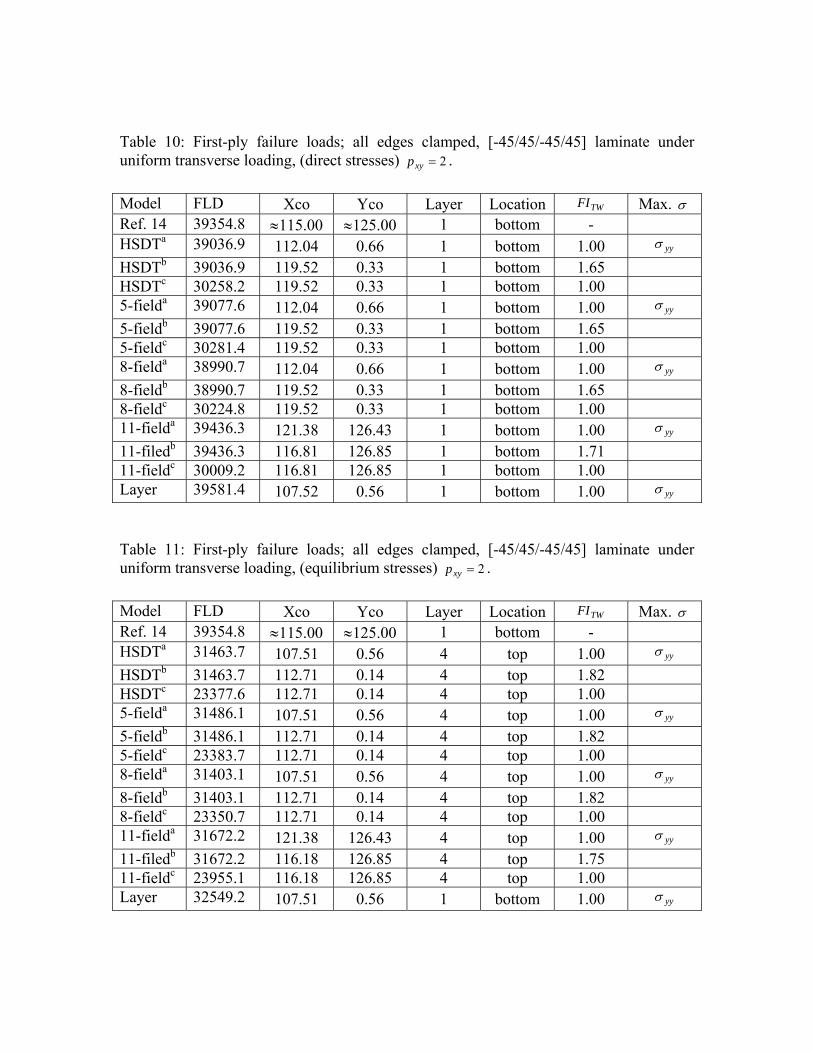
Table 10: First-ply failure loads; all edges clamped, [-45/45/-45/45] laminate under uniform transverse loading, (direct stresses) 2=xyp . Model FLD Xco Yco Layer Location TWFI Max. σ Ref. 14 39354.8 ≈115.00 ≈125.00 1 bottom - HSDTa 39036.9 112.04 0.66 1 bottom 1.00 yyσ

HSDTb 39036.9 119.52 0.33 1 bottom 1.65 HSDTc 30258.2 119.52 0.33 1 bottom 1.00 5-fielda 39077.6 112.04 0.66 1 bottom 1.00 yyσ



11-filedb 39436.3 116.81 126.85 1 bottom 1.71 11-fieldc 30009.2 116.81 126.85 1 bottom 1.00 Layer 39581.4 107.52 0.56 1 bottom 1.00 yyσ

Table 11: First-ply failure loads; all edges clamped, [-45/45/-45/45] laminate under uniform transverse loading, (equilibrium stresses) 2=xyp . Model FLD Xco Yco Layer Location TWFI Max. σ Ref. 14 39354.8 ≈115.00 ≈125.00 1 bottom - HSDTa 31463.7 107.51 0.56 4 top 1.00 yyσ




11-filedb 31672.2 116.18 126.85 4 top 1.75 11-fieldc 23955.1 116.18 126.85 4 top 1.00 Layer 32549.2 107.51 0.56 1 bottom 1.00 yyσ

Table 12: First-ply failure loads; all edges simple supported, [0/90]S laminate under uniform transverse loading, (direct stresses) 2=xyp . Model FLD Xco Yco Layer Location TWFI Max. σ Ref. 14 11646.5 ≈5.00 ≈5.00 4 top - HSDTa 11951.7 115.65 43.66 4 top 1.00 yyσ





Table 13: First-ply failure loads; all edges simple supported, [0/90]S laminate under uniform transverse loading, (equilibrium stresses) 2=xyp . Model FLD Xco Yco Layer Location TWFI Max. σ Ref. 14 11646.5 ≈5.00 ≈5.00 4 top - HSDTa 9948.9 115.46 46.18 4 top 1.00 yyσ




11-filedb 10055.6 117.91 62.67 4 top 1.05 11-fieldc 9786.7 117.91 62.67 4 top 1.00 Layer 11954.4 115.65 43.66 1 bottom 1.00 yyσ

Table 14: First-ply failure loads; all edges simple supported, [-45/45/-45/45] laminate under uniform transverse loading, (direct stresses) 2=xyp . Model FLD Xco Yco Layer Location TWFI Max. σ Ref. 14 32513.5 ≈115.00 ≈65.00 4 top - HSDTa 32367.0 75.09 83.33 4 top 1.00 yyσ





Table 15: First-ply failure loads; all edges simple supported, [-45/45/-45/45] laminate under uniform transverse loading, (equilibrium stresses) 2=xyp . Model FLD Xco Yco Layer Location TWFI Max. σ Ref. 14 32513.5 ≈115.00 ≈65.00 4 top - HSDTa 25802.4 138.28 66.13 4 top 1.00 yyσ



8-fieldb 25687.1 91.91 53.73 4 top 1.08 8-fieldc 24727.7 91.91 53.73 4 top 1.00 11-fielda 30791.5 31.22 0.56 4 bottom 1.00 yyσ


With equilibrium stresses we observe that:

1. For the initial mesh, the failure loads predicted by all the models are lower than those obtained by (Reddy and Reddy, 1992) (shown with superscript a ) and those obtained by using direct stresses.

2. The locations predicted by all the models are either close to one obtained by (Reddy and Reddy, 1992) or are corresponding symmetric points. The locations for both direct stresses and equilibrium stresses are same (or corresponding symmetry points).

3. Failure loads predicted by the HSDT and hierarchic models are close while those predicted by layerwise are slightly higher than these.

4. When the discretization error control is used the failure index, for the failure load obtained using adapted mesh, increases upto 85%. This is due to the increased flexibility of the numerical solution for the adapted mesh.

5. With the adapted mesh the error in the failure load computations can be close to 25%.

6. The failure locations for the HSDT and hierarchic models are in the same region before and after the use of discretization error control.

It is obvious that a suitably refined mesh, along with proper post-processed values of the transverse stresses, is necessary to obtain reliable values of the first-ply failure load. CONCLUSION

1. With respect to pointwise values of transverse deflection and stress, the HSDT and hierarchic models are more reliable for thin plates while for thicker plates these models can lead to erroneous results.

2. The layerwise model accurately captures the local state of stress for all laminated composite plates, for different plate thickness.

3. The in-plane stress components computed by all the models are accurate, for almost all the cases.

4. The in-plane stress components computed by direct use of finite element data for layerwise model are in good agreement with exact one.

5. The transverse stress components computed by direct use of finite element data for HSDT and hierarchic models are significantly different both qualitatively and quantitatively.

6. The equilibrium approach for computing transverse stresses is accurate for all the models.

7. Computed failure load is sensitive to the mesh, order of approximation and model used.

8. When the equilibrium approach for computing transverse stresses is used the

failure load computations can show reduction upto 20%.

9. When the discretisation error is controlled (using focused adaptivity) failure load

computed using direct stresses can go down by more than 23%.

10. When proper discretisation error control is used, failure load computed using

equilibrium approach for transverse stresses the failure load can go down by 25%.

11. From design point of view, proper mesh design is essential, as the actual failure

load can be significantly smaller than the computed one.

12. In general, for symmetric and antisymmetric laminates, the HSDT and hierarchic

models are effective, when equilibrium approach is used to obtain the transverse

stresses.

REFERENCES [1] Reddy, J. N. (1984), A simple Higher order Theory for laminated composite plates, Jl. Appl. Mech,. 51, 745-752. [2] Szabó, B. A. and Sharmann, G. J. (1988), Hierarchic plate and shell models based on p-extension, Int. J. Numer. Methods. Engrg., 26,1855-1881. [3] Babuška, I.,. Szabó, B. A. and Actis, R. L, (1992), Hierarchic models for laminated composites, Int. J. Numer Methods Engrg. ,33, 503-535. [4] Actis, R. L, Szabó, B. A. and Schwab, C. (1999), Hierarchic Models for laminated plates and Shells, Comput. Methods Appl. Mech. Engrg,. 172, 79-107. [5] Ahmed, N. U., and Basu, P. K. (1994), Higher-order finite element modeling of laminated composite plates, Int. J. Numer Methods Engrg., 37, 123-129. [6] Schwab, C. (1996), A-Posteriori Modeling Error Estimation for Hierarchic Plate Model, Numer. Math., 74, 221-259. [7] Verfürth, R. (1996), A review of a-posteriori error estimation and adaptive mesh refinement, New York, Wiley Tuebner. [8] Mohite, P. M. and Upadhyay, C. S. (2002), Local quality of smoothening based a-posteriori error estimators for laminated plates under transverse loading. Computers and Structures, 80(18-19),1477-1488. [9] Mohite, P. M. and Upadhyay, C. S. (2003), Focussed adaptivity for laminated plates. Computers and Structures, 81,287-293. [10] Mohite, P. M. and Upadhyay, C. S. (2004), Accurate computation of critical local quantities in composite laminated plates under transverse loading. Communicated to Computers and Structures. [11] Tsai, S. W. and Wu, E. M.(1971), A general theory of strength for anisotropic materials. Journal of Composite Materials,5,55-80. [12] Pagano, N. J. and Hatfield, S. J. (1972), Elastic behavior of multilayered bidirectional composites. AIAA Journal, 10(7), 931-933. [13] Pagano, N. J. (1970), Exact solutions for rectangular bi-directional composites and sandwich plates, Jl. Composite Materials, 4, 20-35. [14] Pagano, N. J.(1970), Influence of shear coupling in cylindrical bending of anisotropic laminates. Journal of Composite Materials, 4, 330-343. [15] Reddy, Y. S. N., and Reddy, J. N. (1992), Linear and non-linear failure analysis of composite laminates with transverse shear. Composite Science and Technology, 44, 227-255.

COMPARISON OF PLATE MODELS FOR ANALYSIS OF LAMINATED ...home.iitk.ac.in/~mohite/ictacem04.pdf ·...

Documents

Transcript of COMPARISON OF PLATE MODELS FOR ANALYSIS OF LAMINATED ...home.iitk.ac.in/~mohite/ictacem04.pdf ·...