Paper AAS 03-165

COMPARISON OF MSIS AND JACCHIAATMOSPHERIC DENSITY MODELS

FOR ORBIT DETERMINATIONAND PROPAGATION

Keith Akins, Liam Healy, Shannon Coffey, Mike PiconeNaval Research Laboratory

13th AAS/AIAA Space FlightMechanics Meeting

Ponce, Puerto Rico 9-13 February 2003

AAS Publications Office, P.O. Box 28130, San Diego, CA 92198

AAS 03–165

Comparison of MSIS and Jacchia atmospheric

density models for orbit determination and

propagation

Keith A. Akins∗ Liam M. Healy† Shannon L. Coffey‡

J. Michael Picone§

Abstract

Two atmospheric density model families that are commonly chosen for orbit determinationand propagation, Jacchia and MSIS, are compared for accuracy. The Jacchia 70 model, theMSISE-90 model, and the NRLMSISE-00 model may each be used to determine orbits overfitspans of several days and then to propagate forward. With observations kept over the prop-agation period, residuals may be computed and the accuracy of each model evaluated. Wehave performed this analysis for over 4000 cataloged satellites with perigee below 1000km forSeptember–October 1999, and the 60 HASDM calibration satellites with a large observation setfor February 2001. The purpose of this study is to form a picture of the relative merits of thedrag models in a comprehensive view, using all satellites in a manner consistent with the oper-ational practice of US space surveillance centers. A further goal is to refine this knowledge tounderstand the orbital parameter regions where one of the models may be consistently superior.

INTRODUCTION

Precise prediction of satellite motion in low-earth orbits requires significant knowledge of the effectsof the atmospheric drag force. This force has two components which are usually difficult to ascertain:the ballistic coefficient of the satellite, and the atmospheric density at a particular point in its orbit.The problem of atmospheric density has been studied for decades, and two of the most widely-usedatmospheric density models are Jacchia 70 and MSIS.

This paper presents a comparison of orbit determination and propagation results between threeatmospheric density models for over 4000 satellites in low-earth orbit. These satellites represent allthe unclassified satellites with perigees below 1000 km tracked by Naval Network and Space Oper-ations Command (NNSOC, formerly Naval Space Command) in the period of September-October1999. Further analysis is conducted using the HASDM satellite and observation data sets. Thisdata includes 60 primary, or calibration, objects for which a very large number of observations wereaccumulated starting in early 2001.

∗Pennsylvania State University, Aerospace Engineering, University Park, PA 16802, and Naval Research Labora-tory, Code 8233, Washington, DC 20375–5355, E-mail: Keith.Akins@nrl.navy.mil.

†Naval Research Laboratory, Code 8233, Washington, DC 20375–5355. E-mail: Liam.Healy@nrl.navy.mil.‡Naval Research Laboratory, Code 8233, Washington, DC 20375–5355.§Naval Research Laboratory, Code 7643, Washington, DC 20375–5355.

1

DRAG MODELS

An important component of low-earth motion is atmospheric drag, and an important part of de-termining this force is knowledge of the atmospheric density. There are two major families ofatmospheric density models based on empirical data collection in the 1960s, 70s, and 80s. Thesemodels provide estimates of the statistical mean temperature, total mass density, and number den-sity of each species as a function of position, local time, universal time, and solar and geomagneticindices. Of greatest interest to the astrodynamics community is the total mass density.

The two most widely used families of density models are Jacchia, based on the work of LuigiJacchia, and MSIS (Mass Spectrometer — Incoherent Scatter), based on the work of Alan Hedin andcollaborators (Ref. 1). The operational orbit determination community primarily uses the Jacchia 70(J70) model (Ref. 2) while the atmospheric physics community has preferred the MSIS-class models,of which the latest is NRLMSISE-00 (N00) (Ref. 3). To compare the performance of J70 modeland N00 for drag estimation, a discussion of the respective underlying observational data and themethods of generating the models is necessary. For a complete comparison, one must include thepreceding MSIS-class model, MSISE-90 (M90) (Ref. 4). The two MSIS-class models extend fromthe ground (z = 0km) to beyond the exosphere (z ≈ 500 km) while the Jacchia models apply onlyabove 90 km, unless the programmer has augmented the model at lower altitude with either the U.S. Standard Atmosphere (Ref. 5), as is done in the present analysis, or an MSIS representation, asis done in many space surveillance centers.

At thermospheric altitudes (z > 90 km), all three models primarily represent parameterizedsolutions of the equations of diffusive equilibrium for the individual chemical constituents of theatmosphere, such as molecular nitrogen (N2), molecular oxygen (O2), and atomic oxygen (O). Thekey altitude profile parameters for thermospheric variables are the temperature and the temperaturegradient near the inflection point of temperature as a function of altitude (120 − 125 km), theexospheric temperature, and the total mass density and individual species densities at prescribedlower altitudes. In J70, the important parameters are temperature at 90 km and the mixing ratio90 km < z < 105 km; for the MSIS models they are composition and temperature at 120 km. Theseprofile parameters are, in turn, decomposed into harmonic, spherical harmonic, and other termssuch as the dependence of the 10.7 cm solar flux index, F10.7, on density, each with a coefficientto be determined from data. These terms capture dependencies on characteristic temporal andspatial scales, e.g., local time (diurnal-scale tides), UT, day of year (annual-scale cycles), latitude,longitude (not explicit in J70), solar declination (not explicit in M90, N00). The generation of amodel consists of computing the atmospheric densities from observations over a range of the model’sparameters and then doing a nonlinear least squares fit to this density data to derive the coefficients.These coefficients then become the core of the model; they allow the estimation of density givenappropriate input parameters. For a realistic model, the number of coefficients can be quite large;N00, for example, has over 2000 nonzero coefficients.

The oldest of the three models, Jacchia 70, is a fit to a set of density values derived fromorbit observations of satellites covering the time period 1961–1970, falling short of a complete solarcycle. The characteristic fitspans for retrieving density were 1–4 days. Because the region of theperigee dominates the integrated drag over an orbit, Jacchia was able to assign local geophysicaland temporal variables (e.g., solar zenith angle) to the density values. Jacchia then inferred thevarious coefficients in his analytic density model to evaluate the temperature and density profilesas functions of the subroutine arguments (time and location variables, solar index, geomagneticindex). Based on our reading of Jacchia’s reports, his inferences were not the result of a formalmultivariate fitting procedure, but were instead based on a filtering or separation of the individualterms (semiannual variation, diurnal variation, etc.) from the data. It has been found (Ref. 3) thatJ70 does not produce an acceptable representation of his set of data for particular subsets of themodel arguments. Given the computing capability during the 1960s, this is neither an indictment ofJacchia’s work nor a surprise. Rather, one respectfully notes the utility of J70 in operational orbitaldrag estimation.

In the thermosphere, 90 km < z < 500 km, the MSISE-90 model is a Levenberg-Marquardt

2

(nonlinear least-squares) fit to a data set consisting primarily of individual species density valuesand temperature data, as measured by ground-based and satellite-borne systems. The vast majorityof the data covers the two decades prior to 1983, but the fit excluded the total mass density derivedfrom satellite-borne accelerometer data, and orbit determination that Jacchia used. The explicit fitto temperature and individual species density observations has rendered the MSIS-class temperatureand composition estimates demonstrably superior in agreement with direct atmospheric observationsto those of the Jacchia models. An important contributing factor is the use of optimal multivariateassimilation techniques in generating the model; Jacchia apparently did not do this. The atmosphericphysics community has validated the model by direct measurement of the density, for exampleby rocket flights with mass spectrometers, primarily against short time-scale, local measurements,but has not performed similar studies of orbital drag data. These data usually resolve timescalesno shorter than a day and have similarly broader spatial scales, as compared to the N00 inputparameters temperature and number density. We hope that this paper will provide the first step inthat process.

The primary M90 deficiency is the exclusion of data on thermospheric total mass density. TheNRLMSISE-00 model now removes this deficiency by adding extensive data from orbit determination(including Jacchia’s data set) and from accelerometers (Ref. 3). From the standpoint of the modelgeneration data, the N00 model therefore represents an improvement over both M90 (total massdensity) and J70 (composition and temperature). In addition, the superior representation of thetemperature function should translate to superior extrapolation or interpolation of the N00 totalmass density measurements to the conditions of orbital observations. On the other hand, strongtemporal and spatial filtering of density estimates by the orbit determination process could mitigateany potential advantage of N00 to the operational user, depending on the orbit sampling rate andaccuracy.

Our motivation in undertaking this study is primarily to see if the MSIS atmospheric model,with its better representation of the atmosphere, can improve orbit propagation over Jacchia modelstill widely used in the astrodynamics community. Our intent is to examine a broad spectrum ofsatellites, in fact all relevant satellites, and not just a few specially selected ones.

Furthermore, we anticipate, in the net few years, the capability of real-time revision of atmo-spheric density. Research is presently underway examining the effectiveness of modifying the N00model with near real-time, location-specific constituent data to provide a more accurate model.Both the former LORAAS instrument, onboard the ARGOS spacecraft, and the future SSULI in-strument, planned for launch on the the next DMSP spacecraft, gather UV data from limb scansof the atmosphere to determine its composition at the time and location of the scan (Ref. 6). Thiscomposition data is then applied to the base N00 model to produce a better representation of theatmosphere near where the scan was taken. The present study will provide a baseline for evaluatingthe effectiveness of the real-time modified MSIS models.

TEST PROCEDURE

The comparison of atmospheric drag models in the context of satellite orbits makes use of thedetermination of a satellite’s orbit using observations, and the propagation to a time later thanthe range over which observations were taken. Our focus in these studies is not the initial orbitdetermination process (Ref. 7), but rather the orbit estimation, or differential correction, that startswith some state estimate, and provides a new estimate at some later epoch based on a new set ofobservations. As such, it inherently involves propagation, because these observations, the originalepoch, and the new epoch, will be at varied times. As part of this propagation an accurate forcemodel must be used, and hence the need for good knowledge of atmospheric density.

The tests conducted are designed to compare atmospheric density models by looking at howthey affect orbit determination. While we do not have an absolute truth with which to compare ourcomputed result, we can compare one model to the others and identify which is better. For each ofthe satellite sets used, we have a database of observations, initial elements, and the appropriate solar

3

indices, such as F10.7 and the geomagnetic index ap, for the time period in question. Other necessarydata for the functioning of the orbit determination and propagation is present as well. It is importantto note that the solar indices used are the retrospective final values. These are usually not availableuntil some time after the time in question, and have been generated by Air Force Weather Agencyand NOAA after extensive processing of observational data. An orbit determination on current datais different in that the value of these variables are projected into the future and therefore estimated;the final values may differ somewhat. As a result, these tests would be different from a present-timetest because of the use of final values.

Abbreviation NameRST Requested Stop TimeLOBST Last Observation Before Stop TimeGPCD General Pert Catalog DateESC Epoch of Satellite in Catalog

Table 1: Important times in for orbit determination.

Before describing the test procedure, some time terminology must be introduced. The orbitdetermination process requires the use of several different times, and we have given each a name andan abbreviation. These are given in Table 1. First, the user must specify a final time for the orbitdetermination, the requested stop time (RST). This means that no observation after that time willbe used for the orbit determination. Together with a fitspan, this determines the complete range oftimes over which observations may be used. The epoch of the determined vector will not be RST,but rather the time of the last observation before this time, which we call LOBST. Finally, to startthe orbit determination we will need to use an element set from the NNSOC catalog; for conveniencewe give a date to this catalog, general perturbations catalog date (GPCD). More importantly, eachsatellite in this catalog has an epoch, which we call the epoch of satellite in catalog (ESC).

There are two sets of data on which the tests have been performed: all unclassified catalogedsatellites with perigee below 1000 km drawn from a the set of all unclassified observations in theNNSOC (then Naval Space Command) catalog as of October 1999, which we call lowsats, and theHASDM calibration satellites from February 2001. The HASDM satellites were used because of thehigh number of available observations. The disadvantage is that these orbits, while selected to berepresentative of all applicable orbits, still are only a small fraction of the possible orbits affected bydrag. The full catalog of objects with perigees below 1000 km was selected because these were allknown satellites passing through the high drag region and therefore will show how the drag modelaffects operational analysis.

Both the differential correction and the propagation for this project were conducted using theNaval Research Laboratory’s SPeCIAL-K orbit determination software suite (Ref. 8). This software,which is used at NNSOC, uses Special Perturbations (SP) for accurate integration and force mod-eling. The integration for this study was performed using an 8th-order Gauss-Jackson integrator,a 24 × 24 geopotential, and lunar and solar perturbations. Standard observational weighting andbiasing was used, and, for the differential correction, the fitspan was defined, using standard opera-tional algorithms, to be between 1.5 and 10 days based on the mean motion and the rate of changeof mean motion of each object. SPeCIAL-K’s automatic parallel processing capabilities allowed thelarge differential corrections to finish in approximately 4 hours. These runs were completed using13 workers on a variety of computer platforms, including SGI, AIX and Linux.

There are several ways one might consider comparing the validity of an orbit determinationprocess, including, of course, the atmospheric density model. The purpose in doing an orbit deter-mination is to predict the orbit of a satellite, and as such models can be compared by their predictivepower. This process is illustrated in Fig. 1. Additionally, the propagation capabilities of a modelcan be determined by using observations after the initial RST. With these new observations, onecan predict forward and compute residuals, as is shown in Fig. 2. Finally, one can determine a neworbit one day advanced from the first correction and compare the final position with the position

4

Figure 1: A schematic illustration of differential correction test.

Figure 2: A schematic illustration of orbit propagation test.

Figure 3: A schematic illustration of day-to-day test.

5

propagated from the first orbit determination, such as in Fig. 3. Either way, we have a referencetruth based on the observations held in reserve.

INITIAL VECTOR QUALITY

When doing orbit determination by performing a differential correction, one needs an initial vectorupon which to start the correction process. In the case of the tests described here, that comes froma general perturbations element set containing known orbital parameters of the satellite. It may befelt that such an element set is too inaccurate to provide convergence to the correct orbit directly,and so one may consider a process called smoothing. This process consists of the application of orbitdetermination on the initial state vector derived from the element set. By using a force model moreaccurate than general perturbations, including drag, it is hoped that the initial conditions will becloser to the true solution.

An important point is that smoothing will use an atmospheric density model as part of the dragforce calculation. Prior to performing tests of the atmospheric model, we wish to assess the effectof smoothing. Specifically, we were concerned that we might introduce a bias in favor of the dragmodel used for smoothing, assuming all tests were smoothed the same way.

In principle a Newton-Raphson process, which is the essence of differential correction, shouldconverge to the same value regardless of the starting vector, provided the starting point is in thebasin of convergence (Ref. 9) for the solution. Therefore, one might assume that smoothing is anunnecessary step, and further, would not introduce any bias, presuming the basin boundaries didnot change. To test this hypothesis, we performed a test we call “roughing,” which is to take thevector converted from GP elements, add a random vector, and then do a differential correction. Ifthe resulting vectors were the same or similar, one could assume this hypothesis true, and assumesmoothing unnecessary but also non-biasing. The random vector would be chosen from a Gaussiandistribution with a mean of zero and a standard deviation equal to the amount the vector changedin the smoothing calculation.

We chose as the test set the fifty satellites with perigee altitude below 1000 km that had thegreatest number of available observations in the database from September–October 1999. Initially,the corresponding fifty element sets distributed by Naval Space Command on September 29, 1999were converted to state vectors and these vectors were used as the starting points for the differentialcorrection. In this test, GPCD is the day prior to RST; therefore ESC is at least 24 hours beforeLOBST.

Figure 4: Roughing schematic. Once the smoothed vector has been determined, the differencebetween it and the GP vector is used as the standard deviation for the random generation of theroughed vector. The orbit is determined for both that and the original vector, and the ratio of thedifferences of the results formed.

We performed the roughing test on these satellites with the following procedure; see Fig. 4.

6

First, we retrieved catalog elements with a GPCD of 1999-09-29. These were converted to vectorsat ESC. Alternatively, we create the “smoothed” vectors by fitting with observations prior to ESCand using a Jacchia 70 model, propagate the fit vectors to ESC. RST is 1999-09-30 00:00:00.000.Therefore, for each satellite we have two vectors at their ESC, one from the general perturbationspropagation of the element set, and one from a differential correction on the observations using theelement set as the initial vector, the smoothed vector. The important quantity derived from thesmoothed vector is its difference from the general perturbations propagated one. This difference isused as the standard deviation in the generation of a Gaussian noise term to add to the generalperturbations vector.

Orbit determination is performed on each of these two sets of vectors, with the final epoch beingat LOBST with RST being 1999-10-01 00:00:00. For the position and velocity, the vector magnitudeof the difference at this time between these two vectors may be computed, and a ratio formed withthe corresponding vector magnitude of the difference of the roughed initial and the initial GP vector.This ratio is a figure of merit for the roughing test.

We have taken measures to make the differential correction consistent between the baseline andperturbed vector cases. First, we performed the differential correction normally on the baselinecase. During such a run, there are observations that are rejected for a variety of reasons. Theseobservations were then removed from the database for future runs, and the ability for the programto reject observations disabled. This has the effect of insuring that each baseline and perturbed casehas an identical set of reasonable observations. Furthermore, we decreased the convergence toleranceof fractional weighted RMS change from the default 0.01 to 0.001. This means that solving the sameorbit with different input vectors will result in more consistent results because the program quitsiteration on RMS increase as well as decrease, and a decrease of tolerance makes it more likely toget through a “hump” that is often experienced where the RMS increases and then decreases beforeconverging.

The results of this test are given in Figure 5. The bars indicate the range of ratios, and diamondindicates the mean. The results indicate that generally the ratio is quite small, less than 0.1,indicating that the baseline and the perturbed vectors all converge to essentially the same point.There are a few exceptions; notably satellite 25680, for which the ratios are rather large. This isbecause for the baseline case, the differential correction iteration was terminated for reasons otherthan convergence.

Therefore, we conclude that, within reason, perturbations of the initial vector do not affect theresult of the differential correction and therefore smoothing is unnecessary. There are two caveats.First, this assumes the differential correction terminates at convergence. Second, in some cases, ifobservation rejection is not controlled, the set of accepted observations may be different and if so,there could be detectable differences in the resulting fit. There is no reason to believe this biasesthe result towards a particular drag model, however, it therefore also seems unnecessary to performa smoothing operation in the first place.

RMS TEST

Comparing atmospheric models is difficult for a variety of reasons: there is usually no direct mea-surement of density, only the indirect measure from the satellite motion which involves additionalunknowns; models vary in their accuracy over regions of the atmosphere and solar conditions, lead-ing to mixed results depending on the orbit studied; and it is difficult to find a good measure ofaccuracy of orbits.

One way of testing the models’ value to orbit propagation is to examine the residuals. Compar-isons are done by examining the residual errors of both the differential correction and propagationbetween the models. A one-day differential correction is performed with each atmospheric model,and the epoch moved forward by the one day. The final root-mean-squared residual errors are thencompared to evaluate the relative effectiveness of the particular model in a differential correction.The predictive effectiveness of the drag models is then calculated by predicting forward for three

7

Figure 5: Ratios of final position difference to initial position difference.

days and computing the root-mean-squared residual errors at each of the known observations. In ourtest, we included only those satellites that updated in all cases. For the lowsats, the total numberof such satellites included is 4587; for HASDM, all 60 satellites updated.

M90 N00lowsats DC mean −0.00189 −0.00298lowsats DC std. dev. 0.0913 0.0848lowsats Prop. mean −0.0451 −0.0325lowsats Prop. std. dev. 0.271 0.328HASDM DC mean 0.0170 0.0139HASDM DC std. dev. 0.0754 0.169HASDM Prop. mean 0.282 0.142HASDM Prop. std. dev. 0.584 0.456

Table 2: RMS fractional change from J70 to the MSIS models.

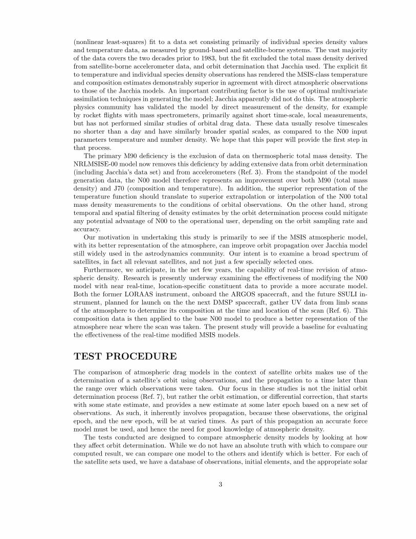
In order to see the effect on differential correction and orbit propagation in changing the modelfrom Jacchia 70 to both MSIS models, we have plotted the fractional change in unweighted RMS thatis computed for each satellite. In Fig. 6 for differential correction and Fig. 8 for orbit propagation,these fractional changes are plotted by satellite in increasing order. With a scatter plot (Fig. 7 fordifferential correction and Fig. 9 for propagation) of the RMS with respect to various fit values, onemay attempt to isolate certain orbits for which one or the other atmosphere model is superior. Nosuch correlation is apparent, although some trends are discernible. The plots for the HASDM set(Figures 10– 13) are qualitatively similar. The RMS fractional change results are summarized inTable 2.

8

Figure 6: Fractional change in unweighted RMS for differential correction by satellite for the lowsatsset, sorted by satellite in order of fractional change.

9

(a) Perigee altitude (b) Eccentricity

(c) Inclination (d) Ballistic coefficient

Figure 7: Fractional change in unweighted RMS in lowsats differential correction plotted againstvarious satellite parameters.

10

Figure 8: Fractional change in unweighted RMS for orbit propagation by satellite for the lowsatsset, sorted by satellite in order of fractional change.

11

(a) Perigee altitude (b) Eccentricity

(c) Inclination (d) B term

Figure 9: Fractional change in unweighted RMS for orbit propagation by satellite for the lowsatsset, plotted against various satellite parameters.

12

Figure 10: Fractional change in unweighted RMS in differential correction by satellite for the HASDMset, sorted in order of fractional change.

13

(a) Perigee altitude (b) Eccentricity

(c) Inclination (d) B term

Figure 11: Fractional change in unweighted RMS in HASDM differential correction plotted againstvarious satellite parameters.

14

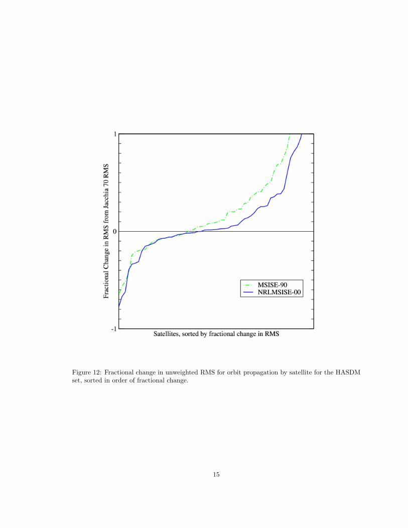
Figure 12: Fractional change in unweighted RMS for orbit propagation by satellite for the HASDMset, sorted in order of fractional change.

15

(a) Perigee altitude (b) Eccentricity

(c) Inclination (d) B term

Figure 13: Fractional change in unweighted RMS for orbit propagation by satellite for the HASDMset plotted against various satellite parameters.

16

ONE DAY ORBIT-TO-ORBIT COMPARISON TEST

The atmospheric models may be compared by the relative predictive power of orbits determinedwith each. Specifically, we determined the orbits using each of three models and observations over aperiod of time ending (RST) at 1999-10-01 00:00:00 for the lowsats set and at 2001-02-15 00:00:00for the HASDM set. Then, we redetermined the orbits 24 hours later, including new observationsduring that additional day. Finally, we propagated each of these determined orbits to the later RSTand compared those positions. Thus, we have an orbit-to-orbit comparison. In our test, we includedonly those satellites that updated in all cases. For the lowsats, the total number of such satellitesincluded is 4423; for HASDM, all 60 satellites updated.

This relative position vector is best presented in the normal, in-track, cross-track coordinatesystem (NTW) (Ref. 7). As one might suspect, most of the error is to be found in the in-trackdirection (Fig. 14(a)), though there can be significant error in the other directions (Figs. 14(b),14(c)) as well. The figures show the distribution of displacement errors for each of the three axesfor each of the three density models. The latter two are almost identically distributed for all threedensity models, and are very symmetric around zero. The distribution is computed by steppingevery two meters, finding how many satellites were within a 10 meters of that value (5 meters forcross track and normal), and dividing by the total population times 10 (5) meters. It thus representsan approximate probability distribution.

To summarize, the means and standard deviations of each component for each drag model inthe lowsats tests are given in Table 3. The distance between the two predicted values gives a scalar

Normal In-track Cross-trackJ70 mean 29.8 493.5 −0.8

J70 std. dev. 1902.4 16592.0 748.8M90 mean 34.1 166.9 −11.8

M90 std. dev. 1941.1 16588.2 820.0N00 mean 40.5 172.1 −11.8

N00 std. dev. 1950.5 16534.3 814.4

Table 3: Mean and standard deviation from orbit-to-orbit test for each drag model in the lowsatsset. Units are meters.

summary of the error for each satellite in each density model.Approximately 0.25% of the lowsats set had very high errors, over 10 km, for each of the density

models. The most prominent among these, for J70 and M90, was satellite 25228, a Russian rocketbody. This was because it decayed in mid-October 1999, shortly after the period that we studied.At the time of study, it was on a reentry trajectory, and its predictability was poor. One couldreasonably expect that this would present a severe test of the drag modeling, and indeed, the resultsobtained showed the one day propagation error to be 2231 km for both J70 and M90. In contrast,the N00 value is 568 km. While too large to be useful, this gives some indication that N00 is betterable to handle reentering satellites. In any case, it has been excluded from all the results above.

Other satellites which had large errors were not in obvious difficult trajectories, but still someerrors were over 100 km. While these were small in number, the large magnitude significantly skewsthe mean and standard deviation position error.

The same test was performed on the HASDM set. Because there are so few satellites in this set,it does not lend itself to a probability density or histogram plot, so we simply summarize the resultsnumerically in Table 4.

CONCLUSIONS

In this paper, we examined the relative accuracy for orbit determination and propagation of threeatmospheric density models, using two sets of data: all the cataloged satellites with perigee below

17

(a) In-track error

(b) Cross-track error (c) Normal error

Figure 14: Distribution of errors in NTW frame of propagated day-old solution relative to newersolution for lowsats (1999) set.

18

Normal In-track Cross-trackJ70 mean −16.4 1365.8 −0.2

J70 std. dev. 34.2 2552.1 21.6M90 mean −7.4 −7.4 8.3

M90 std. dev. 37.8 2224.4 59.0N00 mean −12.6 393.1 3.9

N00 std. dev. 42.4 2128.4 42.0

Table 4: Mean and standard deviation from orbit-to-orbit test for each drag model in the HASDMset. Units are meters.

1000 km, approximately 4500 satellites, and the HASDM calibration set of 60 satellites. In themajority of the tests performed, the MSIS-class models, led by NRLMSISE-00, demonstrate animprovement over the Jacchia model. However, it should be noted that this improvement overall isgenerally very small in light of the variations of the data and that, for the test where Jacchia provedbetter, the differences were also very small. In addition, individual satellites can show markeddifferences, with any of the three models showing the best results. Also, there was no evidencefound to show that one model is better for any subset of the orbital regime, though this deservesmore investigation. In the end, there is no single model which stands out as demonstrably superiorover any other. There is hope, however, that the work currently underway on the implementationof the dynamic NRLMSISE-00 model will change this picture.

ACKNOWLEDGEMENTS

We thank Stefan Thonnard and Andy Nicholas for help with the MSIS model and suggestions ondesign and interpretation of the tests described. MSIS 90 was previously incorporated into SPeCIAL-K by Alan Segerman and Harold Neal.

REFERENCES

[1] Alan E. Hedin. MSIS-86 thermospheric model. J. Geophys. Res., 92:4649–4662, 1987.

[2] L. G. Jacchia. New static models of the thermosphere and exosphere with empirical temperaturemodels. Technical Report 313, Smithsonian Astrophysical Observatory, 1970.

[3] J. M. Picone, A. E. Hedin, D. P. Drob, and A. C. Aikin. NRLMSISE-00 empirical model ofthe atmosphere: Statistical comparisons and scientific issues. J. Geophys. Res., 107(A12):1468,2002.

[4] Alan E. Hedin. Extension of the MSIS thermosphere model into the middle and lower atmosphere.J. Geophys. Res., 96:1159–1172, 1991.

[5] National Technical Information Service, Springfield, Virginia. U.S. Standard Atmosphere, 1976.(Product Number: ADA-035-6000); http://nssdc.gsfc.nasa.gov/space/model/atmos/us_standard.html.

[6] S. Knowles, M. Picone, S. Thonnard, A. Nicholas, K. Dymond, and S. Coffey. Applying newand improved atmospheric density determination techniques to resident space obect prositionprediction. In Advances in Astronautics, San Diego, CA, August 2001. American AstronauticalSociety, Univelt, Inc. AAS 01–426.

[7] David A. Vallado. Fundamentals of Astrodynamics and Applications. McGraw-Hill, New York,1997.

19

[8] Harold L. Neal, Shannon L. Coffey, and Steve Knowles. Maintaining the space object catalogwith special perturbations. In F. Hoots, B. Kaufman, P. Cefola, and D. Spencer, editors, Astro-dynamics 1997 Part II, volume 97 of Advances in the Astronautical Sciences, pages 1349–1360,San Diego, CA, August 1997. American Astronautical Society. AAS 97–687.

[9] William H. Press, Brian P. Flannery, Saul A. Teukolsky, and William T. Vetterling. NumericalRecipes in FORTRAN: The Art of Scientific Computing. Cambridge University Press, 1992.

20