Comparison of Kalman filters in combining panel data from the

1

Research Note RMRS-RN-52. 2013

Rocky Mountain Research Station

Research NoteUnited States Department of Agriculture

Forest ServiceRocky Mountain Research Station

Research Note RMRS-RN-52

June 2013

Comparison of Kalman Filters in Combining Panel Data From the Annual Inventory System of the South Korea

National Forest Inventory

Tzeng Yih Lam, Raymond L. Czaplewski, Jong Su Yim, Kyeong Hak Lee, Sung Ho Kim, Rae Hyun Kim

Citation:

Tzeng Yih Lam, Raymond L. Czaplewski, Jong Su Yim, Kyeong Hak Lee, Sung Ho Kim, and Rae Hyun Kim. 2013. Comparison of Kalman filters in combining panel data from the annual inventory system of the South Korea National Forest Inventory. Res. Note RMRS-RN-52. Fort Collins, CO: U.S. Department of Agriculture, Forest Service, Rocky Mountain Research Station. 15 p.

Authors:

Tzeng Yih Lam (corresponding author)a, Division of Forest Management, Korea Forest Research Institute, Seoul, South Korea.

Raymond L. Czaplewski, Forest Inventory and Analysis Program, Rocky Mountain Research Station, Fort Collins, Colorado.

Jong Su Yim, Kyeong Hak Lee, Sung Ho Kim, Rae Hyun Kim, Division of Forest Management, Korea Forest Research Institute, Seoul, South Korea.aPresent Address: 18, Jalan Sibu 12, Taman Wahyu, Jalan Ipoh, 68100 Kuala Lumpur, Malaysia.

IntroductionNational Forest Inventories (NFIs) serve a primary purpose of providing crucial infor-

mation for formulating national forest policy, environmental planning and reporting to international processes (Tomppo and others 2010). Pressure for timely and reliable forestry statistics urges countries to put a NFI in place or to consider alternative designs. Some countries, for example, USA and Finland, moved from a periodic inventory design to an annual inventory design (Lawrence and others 2010) with the Swedish NFI being one of the earliest examples of the transition (Matérn 1960, Ranneby and others 1987). An annual inventory systematically subdivides a plot network, with equal proportion, into a number of panels equal to the length of measurement cycle (Reams and others 2005). A measure-ment cycle is typically five or ten years. Panels are measured successively on an annual basis. Remeasurement starts in the next cycle once all panels are visited. Thus, an annual inven-tory is expected to meet the demand for continually updated information.

An analytical challenge with annual inventory is deriving accurate and precise estimates of forest statistics for a single year. An unbiased estimate of population mean is the de-sign-based mean estimate from panel data (Van Deusen 2002). However, McRoberts and Hansen (1999) found that the precision of the estimate was unacceptable due to reduced

2


sample size from subdividing total samples into panels. The latter has motivated research in combining time-series of multiple panels to achieve desirable precision. There are a mul-titude of approaches for combining panel data including moving average and temporally different methods (Patterson and Reams 2005), growth models (Lessard and others 2001), time series models (Johnson and others 2003), and mixed estimator (Van Deusen 2002).

Recent development has seen a proliferation of imputation methods for combining panel data (Eskelson and others 2009). The drawback is the requirement for auxiliary informa-tion such as remotely sensed land use classification or climatic variables. With the advent of satellite imagery and airborne sensors, this information could be obtained easily (Czaplewski 1999). However, not all countries—especially developing countries—with the intention of adopting an annual inventory system have the resources to invest in remotely sensed auxiliary information or human resources to process the information. Thus, alternative methods that do not rely on auxiliary information may be more appropriate under such circumstances.

One alternative is the Kalman filter, which is well known in many fields of study, such as aerospace engineering, and economics (Petris and others 2009), but the experience in forest inventory is limited (exception see Dixon and Howitt 1979, Czaplewski 2010). The Kalman filter is a recursive statistical estimator that combines a model prediction and an ob-servation into a weighted average at each calculation step or time increment (Czaplewski and Thompson 2009). In the context of annual inventory, the model describes how a population is expected to change over time, and the observation comes from a panel estimate. Hence, the combination of model- and design-based estimates is expected to reduce risk from model bias and preserve gain in precision from the modeling process (Czaplewski and others 2012). With this advantage, the Kalman filter is potentially an effective method in combining panel data.

The goal of this study was to explore the Kalman filter as an alternative method for com-bining panel data when auxiliary information is not readily available. The study does not attempt to identify a universally best model that applies across any annual inventory. Instead, the objective was to study advantages, disadvantages and application of three specifications of the Kalman filter in contrast to conventional methods of moving average and weight-ed moving average under three populations with different characteristics of change. Each method assumes different rates of change in a population, and therefore, each is a separate hypothesis (Czaplewski and others 2012). This study could be viewed from a perspective of test-of-hypothesis: which model best predicts the trends in population change. Based on these observations, a recommendation is made on possible choice of model for a given set of panel data.

Materials and Methods

DataThis study used the panel data from the 5th South Korea NFI (NFI-5) as a means for mak-

ing comparisons. The NFI program in South Korea was initiated in the early 1960s based on periodic inventory design, but was later enhanced in the fifth session to an annual inventory with new features such as new plot design (Kim 2009). The annual inventory had a measure-ment cycle of five years with the first cycle completed during years 2006 to 2010. A systematic grid of 4 km spacing was overlaid over the whole country, yielding about 4,000 grid points covered by forest. A forest was defined as having a minimum area of 0.5 ha, minimum width of 30 m, crown cover >10% and tree height >5 m (KFRI 2009). The grid points were sys-tematically subdivided into five non-overlapping panels with each panel covering the whole country.

3


A permanent sample plot (PSP) was installed at each grid point. A PSP consisted of four subplots with one at the center and three at 50 m away from the center and at azimuths of 0º, 120º and 240º, respectively (KFRI 2009). Each subplot was a tri-areal plot consisting of three nested circular plots: (1) 0.08-ha plot for trees with diameter at breast height (DBH) ≥30 cm, (2) 0.04-ha plot for trees with 6 <DBH <30 cm, and (3) 0.003-ha plot for saplings and shrubs (KFRI 2009). Observed variables included species, DBH, height, damage, and soil condition, and so on.

This study compared the following provinces in South Korea: Gyeongsangbuk-do, Gyeonggi-do, and Jeju-do. They were chosen for differences in geographical coverage, size, anthropogenic influence, and forest ecosystem. Gyeongsangbuk-do is the largest and the most mountainous province located in the east covering an area of 19,400 km2

and is dominated by Korean red pine (Pinus densiflora S. et Z.). Gyeonggi-do is located in the northwest and ranks fifth in size, but the province has the highest population density. Thus, its dominant coniferous and deciduous forests are influenced by anthropogenic factors. Jeju-do is a volcanic island and the smallest province in the country (1,850 km2) located in the south. Because of distinct parent material and humid subtropical climate, Jeju-do has mostly intact deciduous forest. Due to its small area, a systematic grid of 2 × 2 km was installed to achieve sufficient sampling intensity. The total number of subplots for Gyeongsangbuk-do, Gyeonggi-do and Jeju-do were 3236, 1001, and 536, respectively, of which 20% were measured during any single year.

For each province, the studied variable was mean annual growing stock, that is, volume per hectare (m3/ha). Volume of an individual tree was estimated from volume equations in Kwon and others (2001) and then expanded to per ha by appropriate expansion factors. For each subplot, total volume and volumes of coniferous and deciduous groups were calculated by summing expanded individual tree volume accordingly. Based on the estimated volumes per hectare of the two groups, the subplot was classified into three general forest types: coniferous, deciduous, and mixed forests.

Let ytjk be volume/ha (growing stock) for k-th subplot of j-th forest type in t-th panel, ntj be number of subplots of j-th forest type in t-th panel, and nt be number of subplots in t-th panel, where j = 1,…,3 and t = 1,…,5 (year 2006 to 2010). Estimated mean and variance of growing stock for j-th forest type in t-th panel were

/y y nk

n

1=

= tjktj tjtj/ and

var (( ) ( ) /( ))y y y n n 1tj2= - -tj tjk

k

ntj tj

1=

tj/ ,

respectively. Due to different number of subplots between forest types, the mean and its variance of annual growing stock for t-th panel using methods in Yim and others (2011) were, respectively,

( / )y n n yj 1

3

==

t tj t tj/ (1)

var 2

2 2

( )( )

yn

nvar y

n

n

n

y y

j 1

3

= +-

=t

t

tjtj

t

tj

t

tj t^ h> H/ (2)

where, 3n n=t tj

j 1=/ .

4


The variance estimator assumed each subplot was an independent Primary Sampling Unit, following the procedure in Yim and others (2011). This estimator simplified the cal-culation of mean annual growing stock in this study. Regardless of its statistical properties, this variance estimator was sufficient for comparisons of relative performances among meth-ods and test-of-hypothesis on population. It was not the intention of this study to draw any significant inferences for decision making. Lastly, this estimator reflects the current practice in South Korea while development of variance estimators is in progress. Lastly, yt (Eq. 1) and var yt^ h (Eq. 2) were denoted as single panel estimates at t-th panel (SINGLE), and were inputs to the methods described below.

Moving Average and Weighted Moving AverageThe moving average (MA) is a basic method for combining panel data to increase preci-

sion of current estimate (Roesch and Reams 1999). Due to its simplicity, the method is adopted by several countries implementing annual inventory systems, for example, Sweden NFI program (Axelsson and others 2010). However, MA has often been criticized for lag bias (Johnson and others 2003). Nonetheless, it served as a benchmark comparison in this study. Roesch and Reams (1999) argued that MA might have the tendency to mask tem-poral trends, and they proposed weighted moving average (WMA) whereby more recent panels would receive heavier weights. On this basis, a priori weights were assigned according to Table 1. The rules behind the weight assignment were: (1) the most recent panel received half of the total weight, and (2) weights diminished at a rate of 50% successively. The rules were relaxed for some cases to meet the constraint that total weight summed to one.

First, let y ,WMA t be the WMA estimate of mean annual growing stock for t-th panel,

y w yT

t

1

==

T,WMA t T/ (3)

where wT was the weight assigned to corresponding T-th single panel estimate of mean annual growing stock, and the estimated variance of y ,WMA t was,

var 2vary w y

T

t

1

==

,WMA t T T^ ^h h/ (4)

The MA was a special case of WMA, where for T-th panel, wT = 1/t. Finally, let y ,MA t and var y ,MA t^ h be the MA estimate of mean annual growing stock for t-th panel and its estimated variance, respectively.

Table 1. The a priori weights for weighted moving average (WMA).

t-th Panel

Weights (wT)

w1 w2 w3 w4 w5

1 1.00 – – – –

2 0.40 0.60 – – –

3 0.10 0.30 0.60 – –

4 0.10 0.15 0.25 0.50 –

5 0.03 0.07 0.15 0.25 0.50

5


Kalman FiltersThe Kalman filter resembles a recursive predictor-corrector algorithm for solving a nu-

merical problem, which is analogous to the method of recursive estimation (Pollock 2002, Welch and Bishop 2006). It consists of two sets of equations—prediction equations and correction equations. The prediction equations predict the mean annual growing stock and its error covariance for the time step based on a model of changes in the variable during a single year. The best estimate of mean annual growing stock during the preceding year serves as initial conditions in the model. When a panel estimate of mean annual growing stock and its error covariance are obtained at the next time step, the correction equations are a weighted average of the observed and predicted estimates and error covariances. The more precise estimate receives more weight, and the less precise estimate receives proportion-ally less weight. The correction equations are a generalization of the composite estimator (Gregoire and Walters 1988). Thus, the final estimates consist of a weighted average esti-mate and error covariance for the variable of interest. This procedure is repeated for any number of time steps. For additional information, refer to Maybeck (1979) and Czaplewski and Thompson (2013).

Three Gaussian linear state-space models were studied, that is, random walk plus noise model (WALK), linear growth plus noise model (LINEAR), and exponential growth plus noise model (EXP). A state-space model is a mathematical model representing the underly-ing stochastic process of a system (Czaplewski 2010). A Gaussian linear state-space model is a special case such that the model is a linear function of variables and is built on the normality assumption (Petris and others 2009). Under this assumption, the Kalman filter is a maximum likelihood estimator (Maybeck 1979). The actual computation of a state-space model is complex, but application of the Kalman filter coupled with the normality assumption simplifies the computation significantly (Petris and others 2009). The WALK, LINEAR and EXP were laid out in the state-space model representation.

The state-space model for WALK was (Petris and others 2009),

2

2

, ,

, ,y

w w N

v v N

0

0

+

+

n n v

n v

= +

= +

,

,

t t t w t

t t t t v t

t 1-

^^

hh (5)

where μt and μt–1 were state variables for t- and (t–1)-th panels, vt and wt were normally dis-tributed random errors and assumed uncorrelated, and the estimator of 2

v ,v t was ( )var yt .The second equation of WALK (Eq. 5) specified the stochastic model that the change in

mean annual growing stock was a random process with mean zero over panels (Petris and others 2009). The ratio between the two variances 2 2

/v v, ,w t v t was called signal-to-noise

ratio (SNRWALK), which influenced the performance of WALK (Petris and others 2009). Increasing SNRWALK would weigh the observation heavier in the correction equations of the Kalman filter (Johnson and others 2003). There is no strict rule of assigning a value to SNRWALK; so, it was assumed 0.1 for this study implying that 2

v ,w t was 10% of 2v ,v t .

The state-space model for LINEAR, elaborated from WALK, was (Petris and others 2009),

2

2

2

, ,

, ,

, ,y

w w N

w w N

v v N

0

0

0

+

+

+

n n b v

b b v

n v

= + +

= +

= +

, , ,

, , ,

,

t t t t w t

t t t t w t

t t t t v t

1 1 1 1

1 2 2 2

-

-

t 1-

^``

hjj (6)

where the random errors vt, w1,t and w2,t were assumed normally distributed and uncorrelated.The parameter bt was interpreted as growth rate (Petris and others 2009). Hence,

the stochastic model of LINEAR (last two equations in Eq. 6) implied that current panel

w1,tw2,t

6


population mean annual growing stock nt depended on the previous panel mean an-nual growing stock nt 1- and a rate of change. The latter might change over panels if 2

02vw ,t2. For LINEAR, there were two signal-to-noise ratios, that is, 2 2

/v v ,w v t,t1

(SNRLINEAR1) and 2 2/v v ,w v t,t2

(SNRLINEAR2) (Johnson and others 2003). Both ratios behaved in similar fashion to SNRWALK. For this study, SNRLINEAR1 and SNRLINEAR2 were assumed 0.1 and 0.01, respectively. We assumed a small ratio for SNRLINEAR2 because the data for this study had only five panels and might not be long term enough to detect obvious change in the growth rate bt .

The state-space model for EXP (Czaplewski and Thompson 2013) was specified as,

2

2, ,

, ,y

w w N

v v N

CV0

0

:+

+

n {n

n v

n= +

= + ,

t t t t

t t t t v t

t1 1- -

^^

hh6 @ (7)

where { was exponential growth factor and CV was coefficient of variation.The EXP (where { ≠ 1) resembled WALK (where { = 1) with two exceptions. The pa-

rameter { implied that mean annual growing stock at t-th panel increased by a factor of { from that of (t–1)-th panel. Because of the reforestation effort in the 1950s, forest site con-dition has recuperated and growing stock has increased recently (Lee 2010). Therefore, the assumption of exponential growth was consistent with the past history and anthropogenic influence on the country forests. The { was estimated from the published growing stock statistics from 1981 to 2005 (Korea Forest Service 2010). It was the average of the first dif-ference of the growing stock series; thus, the average { values were 1.058, 1.077, and 1.039 for Gyeongsangbuk-do, Gyeonggi-do and Jeju-do, respectively. Lastly, the variance of the stochastic model implied that underlying stochastic process was assumed heteroscedastic, which is common in many natural systems. For practicality, CV was assumed 0.01.

The results of fitting WALK, LINEAR, and EXP were filtered mean annual growing stock for each method ,y y yand, , ,WALK t LINEAR t EXP t^ h and its associated estimated vari-ance var ( ), var ( and ( ))vary y y, , ,WALK t LINEAR t EXP t^ h for t-th panel.

Bootstrap MethodBootstrap method was used to compare performances of MA, WMA, WALK, LINEAR

and EXP relative to SINGLE for each province. The procedure in the following was de-scribed for a province, but was repeated for all three provinces. At t-th panel, bootstrapping was independently carried out for each of the three forest types, that is, coniferous, decidu-ous and mixed forests. In other words, a sample of ntj subplots was randomly selected with replacement for j-th forest type in the t-th panel. On average, ntj was approximately 216, 67 and 36 subplots for a forest type in one panel for Gyeongsangbuk-do, Gyeonggi-do, and Jeju-do, respectively. Then, Eq. 1 and Eq. 2 were applied to estimate SINGLE for the t-th panel. After that, the five methods (MA, WMA, WALK, LINEAR, and EXP) were fitted with the SINGLE estimates. The sampling and estimation steps were repeated 1000 times for the t-th panel resulting in 1000 estimates of SINGLE, MA, WMA, WALK, LINEAR and EXP. With the bootstrapped estimates, bootstrap average

+yMETHOD t^ h and bootstrap

variance ( )var y+

,METHOD t^ h of mean annual growing stock for a method at the t-th panel

were calculated as

+ +1000 1000 2/ ( ) /andy y var y y y1000 999= = -

+

, , , , , ,m METHOD t m METHOD t METHOD t m METHOD tm1 1= =,METHOD t^ h/ / ,

respectively. Lastly, the above procedure was repeated for each of the five panels.

7


The statistics for evaluating relative performances between methods were mean and standard deviation of errors. For a method and t-th panel, error was defined as the difference between m-th bootstrapped estimate of mean annual growing stock of the method y , ,METHOD t m^ h and the m-th bootstrapped SINGLE estimate y ,t m^ h, that

is, e y y= -, , , ,t m METHOD t m t m for m = 1,…,1000. Thus, mean (ME) and standard deviation (SDE) of the error were 1000

/ME e 1000= ,t t mm 1=/ and

1000 /SDE e ME 999,t m2

= -t tm 1=

^ h/ , respectively. The distribution of et,m for t-th panel and a method was tested for normality with the Shapiro-Wilk test (Shapiro and Wilk 1965). The analysis was done in R open source statistical software (R Development Core Team 2011).

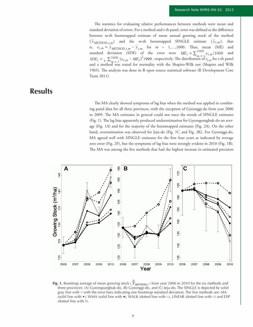
ResultsThe MA clearly showed symptoms of lag bias when the method was applied in combin-

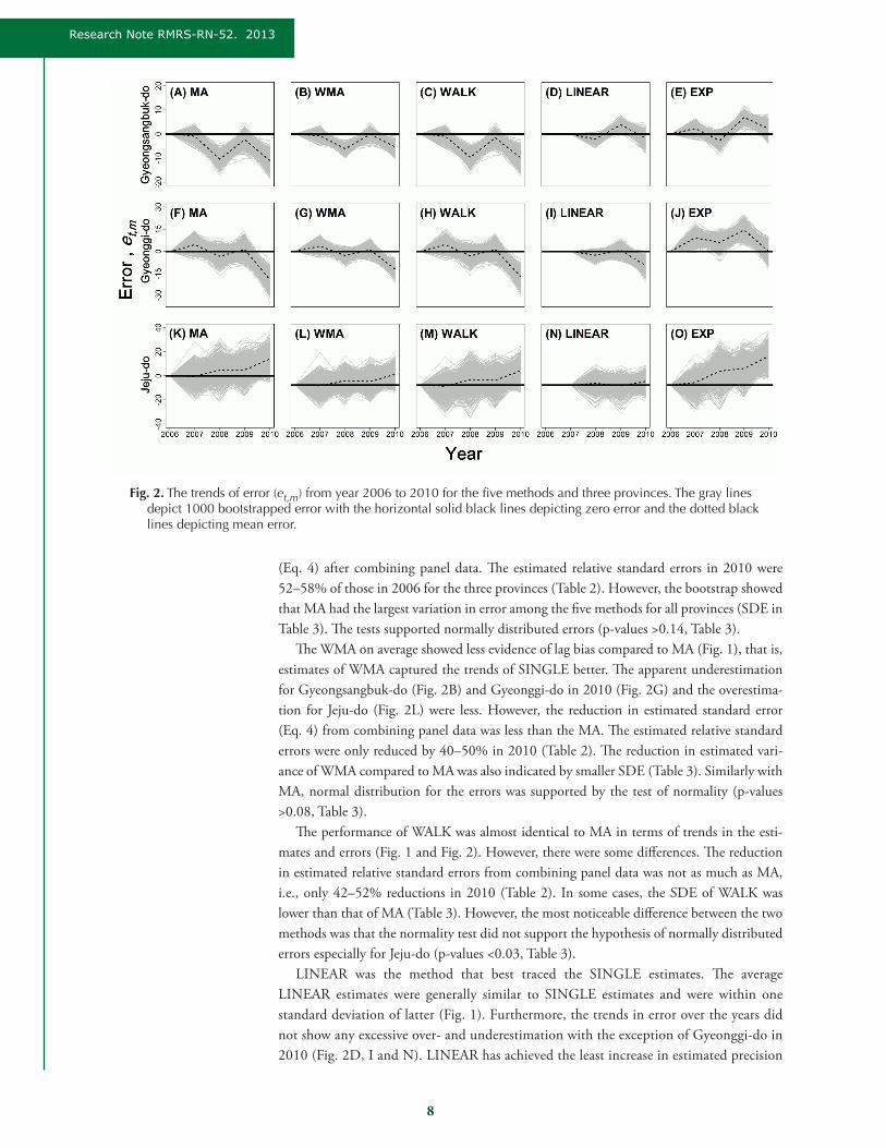
ing panel data for all three provinces, with the exception of Gyeonggi-do from year 2006 to 2009. The MA estimates in general could not trace the trends of SINGLE estimates (Fig. 1). The lag bias apparently produced underestimation for Gyeongsangbuk-do on aver-age (Fig. 1A) and for the majority of the bootstrapped estimates (Fig. 2A). On the other hand, overestimation was observed for Jeju-do (Fig. 1C and Fig. 2K). For Gyeonggi-do, MA agreed well with SINGLE estimates for the first four years as indicated by average zero error (Fig. 2F), but the symptoms of lag bias were strongly evident in 2010 (Fig. 1B). The MA was among the five methods that had the highest increase in estimated precision

Fig. 1. Bootstrap average of mean growing stock ( ,METHOD ty ) from year 2006 to 2010 for the six methods and three provinces: (A) Gyeongsangbuk-do, (B) Gyeonggi-do, and (C) Jeju-do. The SINGLE is depicted by solid gray line with ○ with the error bars indicating one bootstrap standard deviation. The five methods are: MA (solid line with •), WMA (solid line with ■), WALK (dotted line with ○), LINEAR (dotted line with □) and EXP (dotted line with ◊).

8


(Eq. 4) after combining panel data. The estimated relative standard errors in 2010 were 52–58% of those in 2006 for the three provinces (Table 2). However, the bootstrap showed that MA had the largest variation in error among the five methods for all provinces (SDE in Table 3). The tests supported normally distributed errors (p-values >0.14, Table 3).

The WMA on average showed less evidence of lag bias compared to MA (Fig. 1), that is, estimates of WMA captured the trends of SINGLE better. The apparent underestimation for Gyeongsangbuk-do (Fig. 2B) and Gyeonggi-do in 2010 (Fig. 2G) and the overestima-tion for Jeju-do (Fig. 2L) were less. However, the reduction in estimated standard error (Eq. 4) from combining panel data was less than the MA. The estimated relative standard errors were only reduced by 40–50% in 2010 (Table 2). The reduction in estimated vari-ance of WMA compared to MA was also indicated by smaller SDE (Table 3). Similarly with MA, normal distribution for the errors was supported by the test of normality (p-values >0.08, Table 3).

The performance of WALK was almost identical to MA in terms of trends in the esti-mates and errors (Fig. 1 and Fig. 2). However, there were some differences. The reduction in estimated relative standard errors from combining panel data was not as much as MA, i.e., only 42–52% reductions in 2010 (Table 2). In some cases, the SDE of WALK was lower than that of MA (Table 3). However, the most noticeable difference between the two methods was that the normality test did not support the hypothesis of normally distributed errors especially for Jeju-do (p-values <0.03, Table 3).

LINEAR was the method that best traced the SINGLE estimates. The average LINEAR estimates were generally similar to SINGLE estimates and were within one standard deviation of latter (Fig. 1). Furthermore, the trends in error over the years did not show any excessive over- and underestimation with the exception of Gyeonggi-do in 2010 (Fig. 2D, I and N). LINEAR has achieved the least increase in estimated precision

Fig. 2. The trends of error (et,m) from year 2006 to 2010 for the five methods and three provinces. The gray lines depict 1000 bootstrapped error with the horizontal solid black lines depicting zero error and the dotted black lines depicting mean error.

9


Table 2. Average estimated relative standard error (%) of the three provinces for the five panels and the six methods. Relative standard error is estimated as var( ) /y y100 # METHOD, METHOD,t tand is then averaged from 1000 bootstrapped estimates.

Estimation Methods 2006 2007 2008 2009 2010

Gyeongsangbuk-doSINGLE 2.04 2.03 1.79 1.90 2.11MA 2.04 1.44 1.12 0.97 0.88WMA 2.04 1.47 1.27 1.12 1.22WALK 2.04 1.47 1.20 1.10 1.12LINEAR 2.04 2.03 1.67 1.56 1.57EXP 2.04 1.50 1.26 1.21 1.24

Gyeonggi-doSINGLE 3.42 4.05 3.54 4.04 3.29MA 3.42 2.64 2.12 1.88 1.63WMA 3.42 2.76 2.49 2.30 2.09WALK 3.42 2.70 2.26 2.18 2.00LINEAR 3.42 4.05 3.33 3.29 2.76EXP 3.42 2.67 2.21 2.06 1.86

Jeju-doSINGLE 6.27 5.42 6.31 5.58 5.41MA 6.27 4.15 3.48 2.97 2.62WMA 6.27 4.12 4.13 3.34 3.15WALK 6.27 4.15 3.70 3.28 3.01LINEAR 6.27 5.42 5.64 4.87 4.41EXP 6.27 4.11 3.50 3.04 2.75

Table 3. The SDE and p-value from the Shapiro-Wilk test of normality in parenthesis of the three provinces for the five panels and the six methods. Significant p-value (α = 0.05) is in bold and italic.

Estimation Methods 2006 2007 2008 2009 2010

Gyeongsangbuk-doMA 0.00 (–) 1.73 (0.67) 2.05 (0.51) 2.10 (0.14) 2.61 (0.71)WMA 0.00 (–) 1.39 (0.67) 1.28 (0.28) 1.44 (0.15) 1.69 (0.08)

WALK 0.00 (–) 1.68 (0.54) 1.99 (0.39) 1.92 (0.06) 2.54 (0.23)

LINEAR 0.00 (–) 0.00 (–) 1.03 (0.00) 1.26 (0.96) 2.02 (0.06)

EXP 0.00 (–) 1.47 (0.64) 1.70 (0.14) 1.51 (0.06) 2.17 (0.01)

Gyeonggi-doMA 0.00 (–) 3.22 (0.54) 3.71 (0.96) 4.02 (0.67) 4.35 (0.51)WMA 0.00 (–) 2.58 (0.54) 2.35 (0.49) 2.72 (0.20) 2.83 (0.51)

WALK 0.00 (–) 3.23 (0.75) 3.42 (0.59) 3.77 (0.63) 4.07 (0.05)

LINEAR 0.00 (–) 0.00 (–) 1.84 (0.00) 2.69 (0.66) 3.15 (0.02)

EXP 0.00 (–) 3.03 (0.50) 3.28 (0.26) 3.61 (0.31) 3.90 (0.03)

Jeju-doMA 0.00 (–) 6.59 (0.29) 8.09 (0.80) 7.58 (0.89) 7.33 (0.34)WMA 0.00 (–) 5.28 (0.24) 4.93 (0.85) 5.23 (0.45) 4.73 (0.20)

WALK 0.00 (–) 5.57 (0.00) 7.51 (0.00) 6.34 (0.03) 5.64 (0.02)

LINEAR 0.00 (–) 0.00 (–) 4.17 (0.00) 4.44 (0.00) 4.01 (0.02)

EXP 0.00 (–) 5.42 (0.00) 7.49 (0.00) 6.47 (0.07) 5.77 (0.02)

10


from combining panel data; the reduction in estimated relative standard error was merely 20–30% in 2010 (Table 2). When comparing to other methods, LINEAR generally had the smallest SDE. However, the test of normality strongly suggested that errors were not normally distributed for many panels across the three provinces (p-values <0.02, Table 3). However, in absence of normality, the Kalman filter remains a minimum-variance estimator (Maybeck 1979).

The results from EXP fitting were mixed. On average, it adequately captured the trend of SINGLE estimates for Gyeongsangbuk-do but not so for Gyeonggi-do and Jeju-do (Fig. 1). The former was supported by the trends of error for Gyeongsangbuk-do over the years (Fig. 2E). On the other hand, the errors were mostly positive for the other two provinces, especially Jeju-do (Fig. 2J and O), which is an indicator of possible estimation bias. The reduction in estimated relative standard error by EXP covered a wide range, that is, 39–56% in 2010 (Table 2). The SDE of EXP was moderate in most cases and was generally between those of MA and WMA (Table 3). However, there was significant indication of non-normally distributed errors for year 2010 for all three provinces (p-values <0.03, Table 3).

Lastly, estimated relative standard error (Table 2) was compared to bootstrap relative standard deviation (Table 4) to assess the variance estimators of SINGLE, MA, WMA, WALK, LINEAR and EXP var( )y ,METHOD t^ h . In general, the estimated relative standard error of the six methods was similar to or was higher than the corresponding bootstrap relative standard deviation for Gyeongsangbuk-do and Gyeonggi-do for all panels. The former was on average 2-11% higher than the latter. This is evidence for bias in the variance estimators. On the other hand, the estimated relative standard error of the six methods was smaller than the corresponding bootstrap relative standard deviation for Jeju-do with the exception of year 2006 and 2010.

Table 4. Average bootstrap relative standard deviation (%) of the three provinces for the five panels and the six

methods. Bootstrap relative standard deviation is calculated as ,METHOD t

+( ) /var y y100 #

+,METHOD t .

Estimation Methods 2006 2007 2008 2009 2010Gyeongsangbuk-do

SINGLE 1.94 1.95 1.84 1.82 2.10MA 1.94 1.36 1.10 0.95 0.88WMA 1.94 1.39 1.30 1.09 1.22WALK 1.94 1.36 1.13 0.97 0.91LINEAR 1.94 1.95 1.70 1.54 1.50EXP 1.94 1.39 1.15 1.07 1.02

Gyeonggi-doSINGLE 3.18 3.92 3.32 3.73 3.13MA 3.18 2.53 2.00 1.81 1.56WMA 3.18 2.66 2.35 2.20 1.98WALK 3.18 2.51 2.02 1.85 1.64LINEAR 3.18 3.92 3.18 3.11 2.59EXP 3.18 2.55 1.98 1.92 1.63

Jeju-doSINGLE 6.15 5.42 6.67 5.44 5.35MA 6.15 4.16 3.63 3.08 2.67WMA 6.15 4.14 4.41 3.38 3.10WALK 6.15 4.19 3.71 3.13 2.75LINEAR 6.15 5.42 6.03 4.79 4.36EXP 6.15 4.19 3.75 3.18 2.75

11


DiscussionThe MA has been criticized for lag bias especially when a population is changing rap-

idly over time, that is, producing biased estimate of current year’s population parameter (Johnson and others 2003) and underestimation of the variance. Having the largest SDE indicates that accuracy of the method could be very low, suggesting that the method could be unreliable in some instances. On the other hand, Johnson and others (2003) found that MA performed satisfactorily for simulated populations with small to moderate temporal change, which was supported in our study. Hence for a population that remains stable over time, MA could actually be the most suitable method. However, the demand for more current estimates with annual surveys is driven by concern that forest populations are not stable.

Incorporating weights into estimation has evidently allowed WMA to reduce lag bias, at least in this study. Eskelson and others (2009) found that WMA provided improved esti-mates in terms of bias and root mean square error (RMSE) compared to MA. Furthermore, a smaller SDE suggests that WMA could accommodate more variety of trends. Another issue is assigning appropriate weights to panels. Weights are ideally selected based on knowledge of trend inherent in data, but this is generally unknown (Eskelson and others 2009). The choice of weights would affect WMA performance. Arner and others (2004) found that RMSE for mean volume and volume change increased with heavier weighting on recent year rotating panel data from eight states in eastern USA.

The WALK and LINEAR are asymptotically time series autoregressive integrated mov-ing average (ARIMA) models, specifically ARIMA(0,1,1) and ARIMA(0,2,2), respectively (Petris and others 2009). The similar results, especially lag bias, between WALK and MA are supported by the simulation study from Johnson and others (2003). Johnson and others (2003) also found that LINEAR fitted their data too closely and warned that such flexibility might result in the method merely tracking noise rather than any underlying trend. As with selecting weights for WMA, selecting a value for the SNRs of WALK and LINEAR could be as arbitrary (Johnson and others 2003). It depends on the degree of trend smoothing desired. By increasing the SNR, even WALK could match the observed data closely, but with an increase in estimated variances. Lastly, the observed non-normality in error suggests that further study is needed to determine fully the properties of both models.

The EXP takes advantage of state-space model by purposely injecting a priori knowl-edge about underlying process into modeling. It accurately captured the general trend of mean annual growing stock for Gyeongsangbuk-do. Also, it is not surprising that the model performed poorly when the assumed process differed from the observed from year 2006 to 2010 for Jeju-do. This might suggest that historical rate of growth for the province has changed in that period. However, EXP eventually adapted to the observed decreasing trend in mean annual growing stock of Jeju-do in spite of model-misspecification. This illustrates the robust nature of the Kalman filter, where prediction and observation sequentially influ-ence the final estimate. Czaplewski and Thompson (2013) found that a simple Kalman filter model could produce more accurate estimate than MA for rapidly changing popula-tion with detailed residual analysis. Such analysis could detect symptoms of poor model or inaccurate model parameters, and should be studied in future research. Lastly, non-normally distributed errors could affect inference of confidence interval, which is calculated assuming that mean is normally distributed.

This study assumed subplots to be independent and ignored the cluster structure of the 5th NFI inventory design, which was in-line with the current institutional practice.

12


This would likely deflate standard error, which in turn, would inflate precision. In other words, estimated variance var y ,METHOD t^^ hh would be smaller than expected, and boot-strap variance var y+

,METHOD t^^ hh was used as the basis for this comparison. Contrary to the expectation, this was not observed for Gyeongsangbuk-do, Gyeonggi-do and only partially for Jeju-do. This might suggest that the current variance estimator for mean annual growing stock (var yt^ h, Eq. 2) is positively biased for certain populations; however, the cause for the bias is obscure. This highlights the immediate need for further research into variance estimators conforming to the inventory design of the 5th NFI, and to view this study with caution. A proposed future analysis is developing mean and its variance estimators for an-nual growing stock on the cluster level and evaluating the five methods of combining panel data on that level.

Any comparisons of estimated relative standard errors among the methods are con-founded by bias in the variance estimators. MA and WMA are known to suffer from lag bias (Johnson and others 2003), which is also a source of bias in the variance estimators of both methods because the squared error of lag bias is ignored in the estimators. WALK, LINEAR and EXP are model-unbiased (Maybeck 1979), that is, they are unbiased if, and only if, the model predictions are unbiased. However, in the best case, only one of these different model specifications is model-unbiased, and it maybe that they all suffer from model-prediction bias. Hence, even though the estimated relative standard errors for MA were less than the other methods, this does not imply that MA is more precise due to its variance estima-tor not accounting for lag bias. Similarly for WMA, comparisons are confounded by the unknown magnitude of bias in the variance estimators. Comparison in precision between moving average methods and the Kalman filter is tricky because it is confounded by differ-ent types of bias in the variance estimators. Bias is a property of a sample-survey estimator over all possible samples. The true magnitude of bias in any of the methods considered here is unknown because we have only one sample out of very large number of possible samples. Therefore, caution is prudent when comparing estimated relative standard errors among the different methods. All of these estimated relative standard errors are likely biased, and we have no definitive method to determine magnitudes of any of these biases.

The choice of a method for combining a set of panel data from an annualized inventory should consider several criteria: (1) ability to increase precision from combining panel data, (2) inherent number of assumptions, (3) capturing the population underlying process, (4) forecasting, and (5) incorporating data from remeasured panels. All methods in this study produce lower estimated variance. The gain in estimated precision for the Kalman filter depends on model specifications and populations with EXP performing the best for two provinces. The MA and WMA require one assumption in model specification, that is, as-signing weights to panel data, whereas the three Kalman filter methods require at least two assumptions in model specification. Having more assumptions does not necessarily imply a method to be inferior as long as they are justifiable. However, it does require more thought-fulness and defensible arguments. The EXP is the single method that explicitly incorporates knowledge of the underlying process of a population into modeling. Thus, interpretation of the estimates between panels could be directly related to growth. However, the results of Gyeonggi-do and Jeju-do highlighted the need to carefully consider the underlying process. If the underlying process is poorly represented, the resulted model fit will be poor. In con-trast, estimates from the moving average method do not carry such interpretation because measurements between panels are not strictly remeasurements (Czaplewski and Thompson 2013). The ability of the Kalman filter for forecasting has been demonstrated in Petris and others (2009), and one could specify the state-space model to properly take in remeasure-ment data. Specification of the moving average methods do not offer a direct forecasting, and

13


to best of our knowledge, such issue has not been addressed in the literature. Lastly, attempts have been made to modify MA to incorporate remeasured panels (see Van Deusen 2002).

The results did not offer a clear picture on the choice of a method for the 5th South Korea NFI as each method has its advantages and disadvantages. Unless a population is unchanged over time, MA and WMA, and their variance estimators, are known to be bi-ased by design whenever they are used to estimate population variables at one point in time. WALK, LINEAR and EXP are model-unbiased, but only on the condition that the prediction model produces unbiased predictions, and there is little basis for asserting this assumption. Only circumstantial evidence is available to assess the relative degrees of bias among methods, and this evidence is discussed above. Nonetheless, we recommend the Kalman filter over the moving average. This study has demonstrated that the Kalman filter could be specified either as a conventional time series model or a model with hypothesized processes. Because of this flexibility, considerable thought is required to formulate an appro-priate model specification. Furthermore, one has to contend with assumptions associated with the Kalman filter models, for example, values of signal-to-noise ratios (WALK and LINEAR) and a model representing underlying population change (EXP). It is necessary to understand how different ratios and accuracy in representing underlying processes impact model fit for different populations. Estimation of SNR might be possible through analy-sis of residual differences between model predictions and observed estimates (Czaplewski and Thompson 2009), but requires further investigation that is outside the scope of this study. Among the three Kalman filter models, EXP incorporates knowledge of the underly-ing population process, and is beneficial for interpreting results as growth. From another perspective, different model specifications of the Kalman filter can be viewed as test-of-hypothesis regarding characteristics of change in a population; thus, further substantiating our recommendation of the Kalman filter.

More broadly speaking, moving average methods could be a standard method for ana-lyzing a country annual national forest inventory. If the methods fail to provide adequate model fit, it is an indication that the underlying population changes at a drastic rate beyond which could be captured by the methods. Thus, one could then refer to the Kalman filter with different model specifications representing different degrees of change as a test-of-hypothesis on the population underlying rate of change.

AcknowledgmentsWe sincerely thank the Korea Forest Research Institute for the funding to conduct this

research, and the staff of the Division of Forest Resources Information and many oth-ers who have contributed to the 5th National Forest Inventory. The NFI is collaboration among Korea Forest Service, Korea Forest Research Institute, and Forest Inventory Center of National Forestry Cooperatives Federation. We thank Dr. David Turner, Loa Collins and three anonymous reviewers for review of the manuscript.

ReferenceArner, S.L., Westfall, J.A., and Scott, C.T. 2004. Comparison of annual inventory designs

using Forest Inventory and Analysis Data. Forest Science 50(2): 188–203.Axelsson, A.-L., Ståhl, G., Söderberg, U., Peterson, H., Fridman, J., and Lundström, A. 2010.

Sweden. In: Tomppo, E., Gschwantner, T., Lawrence, M., and McRoberts, R.E. (ed.).

14


National forest inventory: pathways for common reporting. Springer Science+Business Media, Heidelberg-Dordrecht-London-New York. p. 541–554.

Czaplewski, R.L. 1999. Multistage remote sensing: toward an annual national inventory. Journal of Forestry 97(12): 44–48.

Czaplewski, R.L. 2010. Complex sample survey estimation in static state-space. Gen. Tech. Rep. RMRS-GTR-239. Fort Collins, CO: U.S. Department of Agriculture, Forest Service, Rocky Mountain Research Station. 124 p.

Czaplewski, R.L., and Thompson, M.T. 2009. Opportunities to improve monitoring of temporal trends with FIA panel data. In: McWilliams, W., Moisen, G., and Czaplewski, R.L. (ed.). Forest Inventory and Analysis (FIA) symposium 2008; October 21-23, 2008; Park City, UT. Proc. RMRS-P-56CD. Fort Collins, CO: U.S. Department of Agriculture, Forest Service, Rocky Mountain Research Station. 58 p.

Czaplewski, R.L., Thompson, M.T., and Moisen, G.G. 2012. An efficient estimator to moni-tor rapidly changing forest conditions. In: Morin, R.S., and Liknes, G.C. (ed.). Moving from status to trends: Forest Inventory and Analysis (FIA) symposium 2012; December 4-6, 2012; Baltimore, MD. p. 416-420. Gen. Tech. Rep. NRS-P-105. Newtown Square, PA: U.S. Department of Agriculture, Forest Service, Northern Research Station. [CD-ROM]. 478 p.

Czaplewski, R.L., and Thompson, M.T. 2013. Model-based time-series analysis of FIA panel data absent re-measurements. Res. Pap. RMRS-RP-102WWW. Fort Collins, CO: U.S. Department of Agriculture, Forest Service, Rocky Mountain Research Station. 13 p.

Dixon, B.L., and Howitt, R.E. 1979. Continuous forest inventory using a linear filter. Forest Science 25(4): 675–689.

Eskelson, B.N.I., Temesgen, H., and Barrett, T.M. 2009. Estimating current forest attri-butes from paneled inventory data using plot-level information: a study from the Pacific Northwest. Forest Science 55(1): 64–71.

Gregoire, T.G., and Walters, D.K. 1988. Composite vector estimators derived by weighting inversely proportional to variance. Canadian Journal of Forest Research 18(2): 282–284.

Johnson, D.S., Williams, M.S., and Czaplewski, R.L. 2003. Comparison of estimators for rolling samples using Forest Inventory and Analysis data. Forest Science 49(1): 50–63.

KFRI. 2009. Field manual of the 5th National Forest Inventory in Korea ver 1.3. Korea Forest Research Institute, Seoul, Republic of Korea. 37 p.

Kim, S.H. 2009. The National Forest Inventory program of Korea: findings and lessons. XIII World Forestry Congress, Buenos Aires, Argentina, 18–23 October 2009.

Korea Forest Service. 2010. Statistical yearbook of forestry. Korea Forest Service, Daejeon, Republic of Korea. 491 p.

Kwon, S.D., Rho, D.K., Lee, K.H., and Son, Y.M. 2001. Timber resources evaluation pro-gram for major species in Korea. KFRI Journal of Forest Science 64: 78–86.

Lawrence, M., McRoberts, R.E., Tomppo, E., Gschwantner, T., and Gabler, K. 2010. Comparisons of national forest inventories. In: Tomppo, E., Gschwantner, T., Lawrence, M., and McRoberts, R.E. (ed.). National forest inventory: pathways for common report-ing. Springer Science+Business Media, Heidelberg-Dordrecht-London-New York. p. 19–32.

Lee, D.K. 2010. Korean forests: lessons learned from stories of success and failure. Korea Forest Research Institute, Seoul, Republic of Korea. 74 p.

Lessard, V.C., McRoberts, R.E., and Holdaway, M.R. 2001. Diameter growth models using Minnesota Forest Inventory and Analysis data. Forest Science 47(3): 301–310.

15


Matérn, B. 1960. Spatial variation—Stochastic models and their application to some problems in forest surveys and other sampling investigations. Meddelanden Statens Skogsforskningsinstitut 49(5): 144.

Maybeck, P.S. 1979. Stochastic models, estimation, and control. Volume 1. Academic Press, New York. 423 p.

McRoberts, R.E., and Hansen, M.H. 1999. Annual forest inventories for the north central re-gion of the United States. Journal of Agricultural, Biological, and Environmental Statistics 4(4): 361–371.

Patterson, P.L., and Reams, G.A. 2005. Combining panels for forest inventory and analysis es-timation. In: Bechtold, W.A., and Patterson, P.L. Gen. Tech. Rep. SRS-80. Asheville, NC: U.S. Department of Agriculture, Forest Service, Southern Research Station. p. 69–74.

Petris, G., Petrone, S., and Campagnoli, P. 2009. Dynamic linear models with R (Use R). Springer Science+Business Media, Heidelberg-Dordrecht-London-New York. 265 p.

Pollock, D.S.G. 2002. Recursive estimation in econometrics. Working Paper No. 462. Department of Economics at Queen Mary, University of London, London. 41 p.

R Development Core Team. 2011. R: A language and environment for statistical computing. R Foundation for Statistical Computing, Vienna, Austria. ISBN 3-900051-07-0. Available at: http://www.R-project.org. [Cited 9 May 2011].

Ranneby, B., Cruse, T., Hägglund, B., Jonasson, H., and Swärd, J. 1987. Designing a new national forest survey for Sweden. Studia Forestalia Suecica 177. Swedish University of Agricultural Sciences, Uppsala, Sweden. 29 p.

Reams, G.A., Smith, W.D., Hansen, M.H., Bechtold, W.A., Roesch, F.A., and Moisen, G.G. 2005. The Forest Inventory and Analysis sampling frame. In: Bechtold, W.A., and Patterson, P.L. Gen. Tech. Rep. SRS-80. Asheville, NC: U.S. Department of Agriculture, Forest Service, Southern Research Station. p. 11–26.

Roesch, F.A., and Reams, G.A. 1999. Analytical alternatives for an annual inventory system. Journal of Forestry 97(12): 33–37.

Shapiro, S.S., and Wilk, M.B. 1965. An analysis of variance test for normality (complete samples). Biometrika 52(3–4): 591–611.

Tomppo, E., Schadauer, K., McRoberts, R.E., Gschwantner, T., Gabler, K., and Ståhl, G. 2010. Introduction. In: Tomppo, E., Gschwantner, T., Lawrence, M., and McRoberts, R.E. (ed.) National forest inventory: pathways for common reporting. Springer Science+Business Media, Heidelberg-Dordrecht-London-New York. p. 1–18.

Van Deusen, P.C. 2002. Comparison of some annual forest inventory estimators. Canadian Journal of Forest Research 32(11): 1992–1995.

Welch, G., and Bishop, G. 2006. An introduction to the Kalman filter. Report TR 95-041. Chapel Hill, NC, Department of Computer Science, University of North Carolina, USA. Available at: http://www.cs.unc.edu/~welch/kalman/. [Cited 9 May 2011].

Yim, J.S., Kim, Y.H., Kim, S.H., Jeong, J.H., and Shin, M.Y. 2011. Comparison of the k-nearest neighbor technique with geographical calibration for estimating forest growing stock volume. Canadian Journal of Forest Research 41(1): 73–82.

The Rocky Mountain Research Station develops scientific information and technology to improve management, protection, and use of the forests and rangelands. Research is designed to meet the needs of the National Forest managers, Federal and State agencies, public and private organizations, academic institutions, industry, and individuals. Studies accelerate solutions to problems involving ecosystems, range, forests, water, recreation, fire, resource inventory, land reclamation, community sustainability, forest engineering technology, multiple use economics, wildlife and fish habitat, and forest insects and diseases. Studies are conducted cooperatively, and applications may be found worldwide. For more information, please visit the RMRS web site at: www.fs.fed.us/rmrs.

Station Headquarters Rocky Mountain Research Station

240 W Prospect RoadFort Collins, CO 80526

(970) 498-1100

Research Locations

The U.S. Department of Agriculture (USDA) prohibits discrimination against its customers, employees, and applicants for employment on the bases of race, color, national origin, age, disability, sex, gender identity, religion, reprisal, and where applicable, political beliefs, marital status, familial or parental status, sexual orientation, or all or part of an individual’s income is derived from any public assistance program, or protected genetic information in employment or in any program or activity conducted or funded by the Department. (Not all prohibited bases will apply to all programs and/or employment activities.) For more information, please visit the USDA web site at: www.usda.gov and click on the Non-Discrimination Statement link at the bottom of the page.

Reno, NevadaAlbuquerque, New MexicoRapid City, South Dakota

Logan, UtahOgden, UtahProvo, Utah

Flagstaff, ArizonaFort Collins, Colorado

Boise, IdahoMoscow, Idaho

Bozeman, MontanaMissoula, Montana

To learn more about RMRS publications or search our online titles:

www.fs.fed.us/rm/publications

www.treesearch.fs.fed.us

Federal Recycling Program Printed on Recycled Paper

You may order additional copies of this publication by send-ing your mailing information in label form through one of the following media. Please specify the publication title and series number.

Publishing Services:Telephone: (970) 498-1392 / FAX: (970) 498-1122E-mail: [email protected] / Web site: http://www.fs.fed.us/rm/

publicationsMailing address: Publications Distribution, Rocky Mountain

Research Station, 240 West Prospect Road, Fort Collins, CO 80526

Comparison of Kalman filters in combining panel data from the

Documents

Transcript of Comparison of Kalman filters in combining panel data from the