Comparison of GRAPE/LBFGS and Krotov in a High … · Grape and LBFGS Krotov Coherent Transfer...

Grape and LBFGSKrotov

Coherent Transfer between Vibrational States in Rb2

Comparison of GRAPE/LBFGS and Krotovin a High-Dimensional Hilbert Space

Michael GoerzFU Berlin

C. Koch Group

OCT Comparison WorkshopCambridge, UK

November 26, 2010

Michael Goerz GRAPE/LBFGS vs. Krotov in a high-dimensional Hilbert Space




9000

12000

15000

18000

21000

24000

ener

gy [

cm-1

]

87 Rb

1Σu

+ (5s + 5p)

# 55, -3642.03 cm-1

5 6 7 8 9 10 11 12 13 14 15 16 17 18 19 20 21 22 23 24 25internuclear seperation [bohr]

0

5000

10000

15000

20000

87Rb X

1Σg

+ (5s + 5s)

# 0, -3814.59 cm-1

# 10, -3252.62 cm-1

# 70, -641.75 cm-1




Outline

1 Grape and LBFGS

2 Krotov

3 Coherent Transfer between Vibrational States in Rb2




Grape and LBFGS




Grape

Acronym

GRAPE: Gradient Ascent Pulse Engineering

optimizations, where the performance can be expressedin terms of the eigenvalues and eigenfunctions of the to-tal propagator.

The paper is organized as follows. In Section 2, wepresent the basic theoretical ideas and numerical optimi-zation algorithms directly applicable to the problem ofpulse design. To illustrate the method, we present threesimple but non-trivial applications to coupled spin sys-tems both in the presence and in the absence of relaxa-tion. In Section 3.1, we look at the problem of findingmaximum coherence transfer achievable in a given timeand the design of pulse sequences that achieve this trans-fer. In Section 3.2, the algorithm is used to find relaxa-tion optimized pulse sequences that perform desiredcoherence transfer operations with minimum losses. InSection 3.3, we design pulse sequences that produce adesired unitary propagator in a network of coupledspins in minimal time. In all examples, we compare theresults obtained by the numerical optimization algo-rithm with optimal solutions obtained by analyticalarguments based on geometric optimal control theory.In the conclusion section, we discuss the convergenceproperties of the proposed algorithm and possibleextensions.

2. Theory

2.1. Transfer between Hermitian operators in the absenceof relaxation

To fix ideas, we first consider the problem of pulse de-sign for polarization or coherence transfer in the absenceof relaxation. The state of the spin system is character-ized by the density operator q (t), and its equation ofmotion is the Liouville–von Neuman equation [15]

_q!t" # $i H0 %Xm

k#1

uk!t"Hk

!

; q!t"

" #

; !1"

where H0 is the free evolution Hamiltonian, Hk are theradiofrequency (rf) Hamiltonians corresponding to theavailable control fields and u (t) = (u1 (t), u2 (t), . . .,um (t))represents the vector of amplitudes that can be changedand which is referred to as control vector. The problemis to find the optimal amplitudes uk (t) of the rf fields thatsteer a given initial density operator q (0) = q0 in a spec-ified time T to a density operator q (T) with maximumoverlap to some desired target operator C. For Hermi-tian operators q0 and C, this overlap may be measuredby the standard inner product

hCjq!T "i # tr Cyq!T "! "

: !2"

(For the more general case of non-Hermitian operators,see Section 2.2). Hence, the performance index U0 of thetransfer process can be defined as

U0 # hCjq!T "i: !3"

In the following, we will assume for simplicity thatthe chosen transfer time T is discretized in N equal stepsof duration Dt = T/N and during each step, the controlamplitudes uk are constant, i.e., during the jth step theamplitude uk (t) of the kth control Hamiltonian is givenby uk (j) (cf. Fig. 1). The time-evolution of the spin sys-tem during a time step j is given by the propagator

Uj # exp $iDt H0 %Xm

k#1

uk!j"Hk

!( )

: !4"

The final density operator at time t = T is

q!T " # UN & & &U 1q0Uy1 & & &U

yN ; !5"

and the performance function U0 (Eq. (3)) to be maxi-mized can be expressed as

U0 # hCjUN & & &U 1q0Uy1 & & &U

yN i: !6"

Using the definition of the inner product (cf. Eq. (2))and the fact that the trace of a product is invariant un-der cyclic permutations of the factors, this can be rewrit-ten as

U0 # hU yj%1 & & &U

yNCUN & & &Uj%1|#####################z#####################kj

j Uj & & &U 1q0Uy1 & & &U

yj|#################z#################

qj

i;

!7"

where qj is the density operator q (t) at time t = jDt andkj is the backward propagated target operator C at thesame time t = jDt. Let us see how the performance U0

changes when we perturb the control amplitude uk (j)at time step j to uk (j) + duk (j). From Eq. (4), the changein Uj to first order in duk (j) is given by

dUj # $iDtduk!j"HkUj !8"

with

HkDt #Z Dt

0

Uj!s"HkUj!$s"ds !9"

Fig. 1. Schematic representation of a control amplitude uk (t),consisting of N steps of duration Dt = T/N. During each step j, thecontrol amplitude uk (j) is constant. The vertical arrows representgradients dU0=duk!j", indicating how each amplitude uk (j) should bemodified in the next iteration to improve the performance function U0.

N. Khaneja et al. / Journal of Magnetic Resonance 172 (2005) 296–305 297

uk (j)

Φ0

original value

at time index j : go in direction of gradient

Pulse Update

uk (j) −→ uk (j)− ε∂Φ0

∂uk (j)




Second Derivative: Newton’s Method

Newton’s method (one-dimensional case)

f (x0 + ∆x) = f (x0) + f ′ (x0) ·∆x +1

2f ′′ (x0) · (∆x)2

df (x0 + ∆x)

d(∆x)= 0 ⇒ xn+1 = xn −

f ′ (xn)

f ′′ (xn)

Newton’s method (multi-dimensional case)

Sequence~xn+1 = ~xn − H−1

f (~xn) · ~∇f (~x0)

converges towards extremum.




Gradient Descent and Newton’s Method

Optimization towards an extremal point by gradient descent (green) and Newton’smethod (red)




Quasi-Newton

Newton’s method (multi-dimensional case)

Sequence~xn+1 = ~xn − H−1

f (~xn) · ~∇f (~x0)

converges towards extremum.

Find matrix B as approximation to H−1 so that B fulfills the secant equation.

Secant Equation

f ′ (x0 + ∆x)− f ′ (x0)

(x0 + ∆x)− x0= B

Underdetermined in higher dimensions! LBFGS is one option to construct B.




Quasi-Newton Algorithms

Quasi-Newton method (general)

Given a ~x0 ∈ RN chosen sufficiently close to a local extremum ~xE of f and an initialguess for the Hessian B0 (for example B0 = I ) repeat the following steps to obtain ~xE :

1 Calculate the step ∆~xk using the current approximated Hessian Bk by:∆~xk = −B−1

k · ~∇f (~xk ).

2 Calculate the new ~xk+1: ~xk+1 = ~xk + ∆~xk .

3 Use the gradient at the new point ~∇f (~xk+1) and the difference in gradients

between new and old point: ~yk = ~∇f (~xk+1)− ~∇f (~xk ) to find a newapproximation for the Hessian Bk+1.

Linesearch

Introduce parameter αk ∈ [0, 1] to modify step size:

∆~xk = −αk · B−1k · ~∇f (~xk )




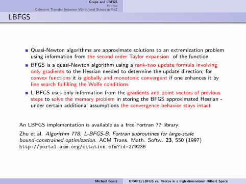
LBFGS

Quasi-Newton algorithms are approximate solutions to an extremization problemusing information from the second order Taylor expansion of the function

BFGS is a quasi-Newton algorithm using a rank-two update formula involvingonly gradients to the Hessian needed to determine the update direction; forconvex functions it is globally and monotonic convergent if one enhances it byline search fulfilling the Wolfe conditions

L-BFGS uses only information from the gradients and point vectors of previoussteps to solve the memory problem in storing the BFGS approximated Hessian -under certain additional assumptions the convergence behavior stays intact

An LBFGS implementation is available as a free Fortran 77 library:

Zhu et al. Algorithm 778: L-BFGS-B: Fortran subroutines for large-scalebound-constrained optimization. ACM Trans. Math. Softw. 23, 550 (1997)http://portal.acm.org/citation.cfm?id=279236


http://portal.acm.org/citation.cfm?id=279236



Calculating the Gradient

Ψin

ε1 ε2 ε3 ε4 ε5

Ψtg

J = −F (Ψ(T )) +

∫ T

t=0ga(ε(t)) dt+

∫ T

t=0gb(Ψ, ε)) dt

F =1

N< tr

O†U(T , 0)

=

1

N<

N∑k=1

⟨Ψtg

∣∣∣U(T , 0)∣∣∣Ψin

⟩ga =

α

S(t)

(ε− εold

)2

Gradient for every pulse value

Gi =∂J

∂εi= −

∂F

∂εi+

∂

∂εi

∑i

α

Si

(εi − εold

i

)2∆t




Calculating the Gradient

Ψin

ε1 ε2 ε3 ε4 ε5

Ψtg

∂

∂ε2F = <

⟨Ψtg

∣∣∣∣∣U5U4U3∂U2

∂ε2U1

∣∣∣∣∣Ψin

⟩; Ui = e−i H(εi )∆t

= <⟨

Ψbw

∣∣∣∣∣∂U2

∂ε2

∣∣∣∣∣Ψfw

⟩

∂Ui

∂εi=

∂

∂εie−i H(εi )∆t

=∞∑

n=1

(−i∆t)n

n!

n−1∑k=0

Hk ∂H(εi )

∂εiHn−k−1




The Basic Idea of Krotov: Convergence by Construction

Ingredients:

final-time target JT [ϕT , ϕ∗T ]

time-dep. targets / costs ga[ε] + gb[ϕ(t), ϕ∗(t)]

equations of motion i~ ∂∂t|ϕ(t)〉 = H(t)|ϕ(t)〉 |ϕ(t0)〉 = |ϕ0〉

Construction of auxiliary functional L

L[ϕ,ϕ∗, ε,Φ] = J[ϕ,ϕ∗, ε]

choose arbitrary scalar potential Φ[ϕ,ϕ∗, t] such that

L[ϕi , ϕ∗,i , εi ,Φ] ≥ L[ϕi+1, ϕ∗,i+1, εi+1,Φ]

building in monotonic convergence




Auxiliary functional L

L[ϕ,ϕ∗, ε,Φ] = G [ϕ(T ), ϕ∗(T )]− Φ[ϕ(0), ϕ∗(0), 0]

−∫ T

0R[ϕ(t), ϕ∗(t), ε(t), t]dt

final-time contribution:

G [ϕ(T ), ϕ∗(T )] = JT [ϕ(T ), ϕ∗(T )] + Φ[ϕ(T ), ϕ∗(T ),T ]

intermediate-time contribution:

R [ϕ(t), ϕ∗(t), ε(t), t] = −(

ga[ε(t)] + gb[ϕ(t), ϕ∗(t)]

)

+∂Φ

∂t+

N∑k=1

[∇ϕk Φ · fk [ϕ,ϕ∗, ε, t]

+∇ϕ∗k

Φ · f ∗k [ϕ,ϕ∗, ε, t]

]




Central Idea of Krotov’s Method

We want a minimum of L, i.e. minimum of G & maximum of Rbut L is changed by both changes in ~ϕ and changes in ε

Krotov’s Solution

(i) choose Φ at the extremum, ~ϕi , such that it is the worst possible choice withrespect to any change in the states y maximize L when going from ~ϕi to ~ϕi+1

for fixed εi

(ii) then any change in the field from εi to εi+1 will lead to a minimization of L

ε(i+1)(t) = arg maxε(t)

R(~ϕ(t)(i+1), ε(t), t

)or

∂R

∂ε

(~ϕ(i+1), ε(i+1), t

)= 0 ,

∂2R

∂ε2

(~ϕ(i+1), ε(i+1), t

)< 0




Pulse Update by Krotov

Krotov Update Formula

∆ε(t) =S(t)

α=[

N∑k=1

ak

⟨Ψin,k

∣∣∣O†U†(T → t, ε(i))µU(0→ t, ε(i+1))∣∣∣Ψin,k

⟩]

interference between past andfuture events

0 t T

fϕ0ε

ϕiε1

∆ε(t)




Second Order Krotov

Second Order Krotov Update Formula

∆ε(t) =S(t)

α=[

N∑k=1

⟨χ

(i)k (t)

∣∣∣∣∣∂H

∂ε

∣∣∣∣∣φ(i+1)k (t)

⟩← first order

second order→ +σ(t)

2

N∑k=1

⟨∆φ

(i+1)k (t)

∣∣∣∣∣∂H

∂ε

∣∣∣∣∣φ(i+1)k (t)

⟩]

Second Order σ(t)

σ(t) =

eB(T−t)

(CB− A

)CB

for B 6= 0

C(T − t)− A for B = 0

Daniel Reich, Mamadou Ndong and Christiane P. KochMonotonically convergent optimization in quantum control using Krotov’s method.

arXiv:1008.5126




Coherent Transfer between VibrationalStates in Rb2





9000

12000

15000

18000

21000

24000

ener

gy [

cm-1

]

87 Rb

1Σu

+ (5s + 5p)

# 55, -3642.03 cm-1

5 6 7 8 9 10 11 12 13 14 15 16 17 18 19 20 21 22 23 24 25internuclear seperation [bohr]

0

5000

10000

15000

20000

87Rb X

1Σg

+ (5s + 5s)

# 0, -3814.59 cm-1

# 10, -3252.62 cm-1

# 70, -641.75 cm-1




Questions for LBFGS

Cost Functional

J = −⟨

Ψtg

∣∣∣U(T , 0)∣∣∣Ψin

⟩+

∫ T

t=0ga(ε(t)) dt

Can I include the running cost?

Which order of the gradient do I need?

How much does LBFGS improve on Grape?

How does LBFGS compare to Krotov?




Simple Problem: v = 10 → v = 0




Running cost with LBFGS (v = 10 → v = 0)

0

0.2

0.4

0.6

0.8

1

0 100 200 300 400 500

1−

J

iteration

α = 0

α = 0.01

α = 12




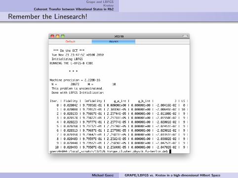
Remember the Linesearch!





0

0.2

0.4

0.6

0.8

1

0 100 200 300 400 500

1−

J

iteration

α = 0

α = 0.01

α = 12

adjusted for LS, α = 0

adjusted for LS, α = 0.01





Order of the Gradient in LBFGS (v = 10 → v = 0)

0

0.2

0.4

0.6

0.8

1

0 100 200 300 400 500

1−

J

iteration

3rd order grad

2nd order grad

1st order grad

0.98

0.985

0.99

0.995

1

0 100 200 300 400 500




LBFGS vs Grape (v = 10 → v = 0)

0

0.2

0.4

0.6

0.8

1

0 100 200 300 400 500

1−

J

iteration

LBFGS 3rd order grad

Grape 3rd order grad




Krotov vs LBFGS (v = 10 → v = 0)

0

0.2

0.4

0.6

0.8

1

0 100 200 300 400 500

1−

J

iteration

Kotov 1

LBFGS (3rd order grad)

LBFGS adjusted for LS (3rd order grad)

0.98

0.985

0.99

0.995

1

0 100 200 300 400 500




Can I include the running cost? — No

Which order of the gradient do I need? — At least second order

How much does LBFGS improve on Grape? — A lot. (Forget about Grape)

How does LBFGS compare to Krotov? — Not too shabby




More Advanced Problem: v = 70 → v = 0





0

0.2

0.4

0.6

0.8

1

0 100 200 300 400 500

1−

J

iteration

α = 0

α = 0.01

α = 12





0

0.2

0.4

0.6

0.8

1

0 100 200 300 400 500

1−

J

iteration

α = 0

α = 0.01

α = 12


adjusted for LS, α = 0.01





LBFGS vs Grape (v = 70 → v = 0)

0

0.2

0.4

0.6

0.8

1

0 100 200 300 400 500

1−

J

iteration

LBFGS 3rd order

Grape 3rd order




Order of the Gradient in LBFGS (v = 70 → v = 0)

0

0.2

0.4

0.6

0.8

1

0 100 200 300 400 500

1−

J

iteration

3rd order grad

2nd order grad

1st order grad

0.98

0.985

0.99

0.995

1

0 100 200 300 400 500




Krotov vs LBFGS (v = 70 → v = 0)

0

0.2

0.4

0.6

0.8

1

0 100 200 300 400 500

1−

J

iteration

Krotov 1

LBFGS (3rd order grad)

LBFGS adjusted for LS (3rd order grad)

0.98

0.985

0.99

0.995

1

0 100 200 300 400 500




Krotov Second Order

20

0 50 100 150 200 250iteration

0.0

0.2

0.4

0.6

0.8

1.0

-JT

first orderA = 0.001A = 0.01A = 0.1A = 0.2 A = 2 A(!")

50 100 150 200 250

0.99

1.00

0 1 2 3 40.00

0.10

FIG. 2: (color online) Convergence of the first order and sec-ond order constructions of the optimization algorithm as mea-sured by the final-time objective, JT , for state-to-state trans-fer from vibrational level v = 10 to v = 0.

investigate the optimization of a state-to-state transfer,i.e. we have N = 1. The vibrational eigenstates v =10 and v = 0 of X1Σ+

g (5s + 5s) are chosen as initialand target states, respectively. The vibrational periodof the initial state is about 614 fs; we therefore fix theoptimization time to T = 1 ps. The central frequencyis taken to be Ω = ωv=10→v=0, and the maximum fieldamplitude is set to 0 = 1 · 10−2 a.u.

The convergence of the final-time objective JT is shownin Fig. 2, comparing first order (black circles) and sec-ond order constructions of the algorithm. A numberof choices for the second order construction is possible.Since the supremum estimation of A yields zero for bi-linear final-time costs, A can be taken to be equal tosome small positive number, εA, cf. Eq. (79) (dottedand dashed lines in Fig. 2). Alternatively, A(∆ϕ) canbe calculated according to Eq. (80a), cf. solid red linein Fig. 2. The latter choice might speed up convergence,but is more risky: Since A = 2A(∆ϕ) can become neg-ative, the condition for monotonic convergence may beviolated. This is clearly seen in Fig. 2. In the lower in-set, monotonic convergence is lost for one step after thefirst iteration step. We find in this case, that the statechange is almost maximal, |∆ϕ| = 1.95 ≤ 2, i.e. theworst possible case that the optimization algorithm mustdeal with is reached. While the first order constructionconverges faster initially, the upper inset shows that allsecond order constructions supersede the first order oneas the optimum is reached. This is readily understoodby inspection of Eq. (81): The first order contributionto the change in the field is closely related to the gra-dient of the functional which vanishes close to the opti-mum. Variation of the small positive number, εA, showsthat an optimal choice of εA exists. However, this opti-mal choice cannot be determined a priori. In terms ofconvergence speed close to the optimum, it is thereforerecommendable to choose A in terms of A(∆ϕ). Sucha choice effectively makes use of the history of the opti-

0 100 200 300 400 500iteration

0.0

0.2

0.4

0.6

0.8

1.0

-JT

first orderA = 0.001A = 0.01A = 0.1A = 0.2A = 2A(!")

100 200 300 400 500

0.97

0.98

0.99

1.00

FIG. 3: (color online) Convergence of the first order and sec-ond order constructions of the optimization algorithm for aHadamard gate of the lowest two vibrational levels of the elec-tronic ground state.

mization through ∆ϕ.Second, we investigate the optimization of a unitary

transformation. Our target is taken to be the Hadamardgate on the lowest two vibrational eigenstates of the elec-tronic ground state potential,

O =1√2

1 11 −1

,

hence N = 2, and the trace in Eq. (2) is evaluatedover |e = 1, v = 0 and |e = 1, v = 1. The conver-gence behavior for this final-time cost is shown in Fig. 3.The same values for the parameter A as in Fig. 2 aretested. Optimizing a unitary transformation representsa more difficult control problem than state-to-state opti-mization. Therefore the fidelities after 500 iteration stepsin Fig. 3 are smaller than those after 250 steps in Fig. 2.There also exists an optimal choice for εA, cf. Eq. (79),but this choice differs for the two optimization problems.This suggests that different optimal εA may be foundfor each specific optimization problem. However, in bothcases the most efficient optimization strategy is given byA = 2A(∆ϕ), i.e. the solid red lines in Figs. 2 and 3,cf. Eqs. (79) and (80a). We therefore conclude that thisrepresents the recommended choice of A.

C. Bilinear final-time cost and state-dependentintermediate-time cost

We now turn to optimizing the state-to-state trans-fer from v = 0 to v = 1 and the Hadamard gate ofthe previous section taking into account an additionalstate-dependent cost, gb. If both a state-dependent costand a final-time target are present, the algorithm seeksto optimize a compromise between the two goals. Theparameters λ0 and λb determine the relative weight ofeach target. Monotonic convergence always refers to thevalue that the total functional, J of Eq. (1), takes; and

21

each separate contribution to J does not need to con-verge monotonically. Below we will discuss convergenceof both J and JT . In order to render the optimal valueof J independent of the choice of the weights λ0, λb, wedefine a normalized functional,

Jnorm =J

λb − λ0, λb ≤ 0 , (84a)

Jnorm = 1 − J − λ0

λb − λ0, λb ≥ 0 , (84b)

that converges toward one.The cost gb is employed to avoid any population trans-

fer to a forbidden subspace, taken to be the 1Πg(5s+4d)state [35]. In other words, throughout the complete timeinterval, [0, T ], the population shall evolve in the allowedsubspace formed by the X1Σ+

g (5s+5s) and 1Σ+u (5s+5p)

states. This can be expressed by taking the operator Din Eq.(4) to be one of the two choices,

D = Pallow = |e1e1| + |e2e2|, λb ≤ 0 (85a)

D = Pforbid = |e3e3|, λb ≥ 0 , (85b)

where Pallow and Pforbid denote the projectors onto theallowed and forbidden subspaces, respectively. The dif-ferent signs of the weight λb indicate maximization forPallow and minimization for Pforbid.

Choosing gb as expectation value of a projection oper-ator, the analytical estimate for the parameter C of thesecond order contribution is given by Eq. (57). However,let us write explicitly ∆2 of Eq. (15) for the case that theoptimization algorithm is constructed only to first order,

∆2 = −λb1

T

T

0

1

N

N

k=1

∆ϕk|D|∆ϕk dt .

For D = Pallow, the necessary condition for monotonicconvergence, ∆2 ≥ 0, is always fulfilled. A second orderconstruction is therefore not required [35], correspond-ing to C = 0. This is in accordance with Eq. (57) whichyields a large positive number and C in this case is deter-mined by −εC , cf. Eq. (79), where εC is a small positivenumber. Of course, one can employ a second order con-struction for D = Pallow and check whether this improvesconvergence. If, on the other hand, the projector onto theforbidden subspace is assumed in gb, ∆2 ≥ 0 is not neces-sarily fulfilled and a second order construction is requiredto ensure monotonic convergence. Eq. (57) now yields alarge negative number for C since λb is negative, and Cis determined by C.

In the calculations presented below, the final time isset to T = 2 ps, the central frequency of the guess fieldis chosen to be Ω = ωv=0→v=10 and 0 = 2 · 10−4 a.u.Since the emphasis is on the choice of the parameter C,A is taken to be zero.

As in the previous subsection, we first investigateoptimization of a state-to-state transfer. The resultsare shown in Fig. 4 for D = Pallow and in Fig. 5 for

0 200 400 600 800 1000 1200iteration

0.0

0.2

0.4

0.6

0.8

1.0

-JT

first orderC = -0.02C = -0.2 C = -2C = 2C(!")

800 1000 1200

0.990

0.995#b = -20

FIG. 4: (color online) Convergence of the first order and sec-ond order constructions for state-to-state transfer with state-dependent cost. The operator D is taken to be the projectoronto an allowed subspace, i.e. the second order constructionis not required.

1500 2000

0.99

1

0

0.2

0.4

0.6

0.8

1

-JT

first order, !b = 1first order, !b = 20C = -0.5 !b/NT, !b = 20C = - !b/NT, !b = 20C = 2C("#), !b = 20

0 500 1000 1500 2000iteration

00.20.40.60.8

1

J norm

0 50 100 150

0.9

0.95

1

J norm

0 50 100 1500

0.20.40.60.8

1

-JT

FIG. 5: (color online) Convergence of the first order and sec-ond order constructions for state-to-state transfer with state-dependent cost. The operator D is taken to be the projectoronto a forbidden subspace, i.e. the second order constructionis required.

D = Pforbid. While a second order contribution is notrequired in Fig. 4, it can be included by taking C to beequal to −εC , where εC is a small positive number, cf.Eq. (79) (dotted and dashed lines in Fig. 4). This choiceof C does not affect monotonicity. However, it also doesnot yield a faster convergence than the first order algo-rithm. Alternatively, we can take C = 2C(∆ϕ) whereC(∆ϕ) is calculated according to Eq. (80c). NeglectingεC in Eq. (79) is somewhat risky and this choice of Cdoes not guarantee monotonic convergence since C(∆ϕ)can become positive. Indeed, the small ripples in the redsolid line in Fig. 4 illustrate some violation of monotonic-ity. However, this is more than compensated for by theimproved speed of convergence as compared to the firstorder and the conservative choices of C in terms of εC .

Daniel Reich, Mamadou Ndong and Christiane P. KochMonotonically convergent optimization in quantum control using Krotov’s method.arXiv:1008.5126




Conclusions

Use LBFGS if gradient can be calculated easily. Watch the number oflinesearches if propagation is expensive.

Make sure the gradient is exact enough (at least second order)

Use Krotov second order when cost functional requires it, e.g. withstate-dependent costs.

Combine Krotov with LBFGS?




Thank You!

AG Koch — Moving from Berlin to Kassel!

Christiane Koch, already at Kassel

Daniel Reich

Mamadou Ndong, now at Laboratoire de Chimie Physique d’Orsay

Ruzin Aganoglu

Anton Haase


Comparison of GRAPE/LBFGS and Krotov in a High … · Grape and LBFGS Krotov Coherent Transfer...

Documents

Transcript of Comparison of GRAPE/LBFGS and Krotov in a High … · Grape and LBFGS Krotov Coherent Transfer...