COMPARISON OF FLOYD-WARSHALL AND MILLS ALGORITHMS … · the Floyd-Warshall and Mills are 1057.22...

International Journal of Physical Sciences Research

Vol.3, No.1, pp.35- 52, February 2019

___Published by European Centre for Research Training and Development UK (www.eajournals.org)

35 ISSN: Print ISSN 2515-0391, Online ISSN 2515-0405

COMPARISON OF FLOYD-WARSHALL AND MILLS ALGORITHMS FOR

SOLVING ALL PAIRS SHORTEST PATH PROBLEM: CASE STUDY OF SUNYANI

MUNICIPALITY

a Daniel Ashong, b K. F. Darkwah, c Helena Naa Kokor Tetteh,

a. Tutor, Department of Mathematics and ICT, Berekum College of Education, Ghana.

b. Senior Lecturer, Department of Mathematics, Kwame Nkrumah University of Science

and Technology, Ghana.

c. Tutor, Department of Mathematics and ICT, Berekum College of Education, Ghana.

ABSTRACT: The Floyd-Warshall and Mill algorithm were used to determine the all pair

shortest paths within the Sunyani Municipality so as to compare which of the algorithms runs

faster on the computer. The two algorithms were used on a network of 80 nodes with respective

edge distances in matrix format as inputs. Matlab codes were generated to run the algorithms.

All the two algorithms were able to compute the all pair shortest paths. The running time for

the Floyd-Warshall and Mills are 1057.22 and 444.53 ( in seconds ) respectively. The two

algorithms computed the shortest path from node 1 (Ohunukurom) to node 80 (Addae Boreso)

to be 17.3000 km. Based on this study, it is convenient to conclude that Mills decomposition

algorithm runs more faster on a computer than the Floyd-Warshall algorithm.

KEYWORDS: Node, Algorithm, Shortest path, running time, Infinite, Computations

INTRODUCTION

In recent times the world has become a global village and for that matter information can

quickly be shared throughout the world. It has become important to provide information which

will make travelling in our communities easier. Individuals from different fields of academia

have contributed to this development. More importantly, mathematicians have come out with

different algorithms to address this problem. The mathematical algorithms serve as the tools

for mathematicians. The mathematician needs efficient tools to work with, that is the tool

should be able to execute the task in the required or reduced time frame. This means the

mathematician should be time conscious when developing or choosing an algorithm to solve a

problem. Time management is important in all fields of work, especially in the mathematical

world.

According to Kleinschmith (2010), ‘if you want to succeed, if you want to live a life to be

proud of, then you need to make the most of your time’. This means to make it to the top,

today’s mathematician needs outstanding time management skills.

Time management is the act or process of exercising conscious control over the amount of time

spent on specific activities, especially to increase efficiency or productivity. Time management

may be aided by a range of skills, tools, and techniques used to manage time when

accomplishing specific tasks, projects and goals. This set encompasses a wide scope of

activities, and these include planning, allocating, setting goals, delegation, analysis of time

spent, monitoring, organizing, scheduling, and prioritizing. Initially, time management referred

to just business or work activities, but eventually the term broadened to include personal

http://www.eajournals.org/

http://en.wikipedia.org/wiki/Management

http://en.wikipedia.org/wiki/Planning

http://en.wikipedia.org/wiki/Allocating

http://en.wikipedia.org/wiki/Goal_setting

http://en.wikipedia.org/wiki/Monitoring





activities as well. A time management system is a designed combination of processes, tools,

techniques, and methods. Usually time management is a necessity in any project development

as it determines the project completion time and scope. (Wikipedia, 2011). This means the time

factor is very important in choosing a tool and technique or an algorithm to work with.

According to (Mills, 1966), the methods of solving shortest path problems are classified into

two groups: the tree method and the matrix method. The objective of this study is to investigate

two of the matrix methods (Floyd-Warshall algorithm and Mills decomposition algorithm) to

establish which method has the fastest running time on the computer.

LITERATURE REVIEW

Introduction to Mathematical Networks

According to Hillier and Lieberman (2000), network arises in numerous settings and in a

variety of guises. Transportation, electrical, and communication networks pervade our daily

lives. Networks representations are widely used for problems in such diverse areas as

production, distribution, project planning, facility location, resource management and financial

planning to name just a few examples. It is also important to note that, a network representation

provides such a powerful visual and conceptual aid for portraying the relationships between

the components of systems that is used in virtually every field of Scientific, Social, and

Economic endeavour. One of the most exciting developments in Operation Research (OR) in

recent years has been the unusually rapid advance in both the methodology and application of

network optimization models. A number of algorithmic breakthroughs have had a major

impact, as have ideas from computer science concerning data structures and efficient data

manipulation. Consequently algorithms and software now are available and are being used to

solve huge problems on a routine basis that would have been completely intractable two or

three decades ago.

Hiller and Lieberman again in the same year gave brief description about networks. According

to them, a network consists of points and a set of lines connecting certain pairs of the points.

The points are called nodes (or vertices) while the lines are called arcs (or links or edges or

branches). In a network the arcs corresponds to the roads in the system. Arcs are labelled by

naming the nodes at the either end. Let the distance between two nodes 𝑖 and 𝑗 be 𝑑𝑖𝑗. where 𝑖

is the starting or source node and 𝑗 is the end or destination node. Comparing with this study

for example, the villages and towns are the nodes, whiles the roads are the arcs. They also

pointed out that, basically there are two types of networks.

(a) The directed arcs network: when the flow or movement through an arc is allowed in only

one direction. The direction is indicated by adding an arrow head at the end of the line

representing the arc.

(b) The undirected arcs network: when the flow through an arc is allowed in either direction. It

is important to note that undirected network can be converted to directed network and vice

versa. When two nodes are not connected by an arc, it means there is no direct connection

between those two nodes and it is represented as very large or infinite (∞) distance.

Rabbani (2008), presented a distribution network design problem in a multi-product supply

chain system that involves locating production plants and distribution warehouses as well as

determining the best strategy for distributing the product from plants to warehouses and from

the warehouses to customers. The goal is to select the optimum numbers, locations and






capacities of plants and warehouses to open, so that all customer demands of all product types

are satisfied at minimum total costs of the distribution network. Unlike most of the previous

researches, the study considered a multi-product supply chain system. A mixed-integer

mathematical programming model for designing a supply chain distribution network was

developed. Finally, the study presented a real-case study to investigate designing a

pharmaceutical supply chain distribution network.

Takahashi (2002), also presented a study which develops a mathematical framework for

solving dynamic optimization problems with adaptive networks (AN's) based on Hopfield

networks. The dynamic optimization problem (DOP) includes a dynamic travelling salesman

problem (TSP), in which the distance between any pair of cities in the conventional TSP is

extended into a time variable. Compared to previous deterministic networks, such as the

Hopfield network, the adaptive network has the most distinguished feature: it can change its

states, continually reacting to inputs from the outside environment. From the scientific

viewpoint, the framework demonstrates mathematically rigorously that the adaptive network

produces as final states locally minimum solutions to the DOP. From the engineering

viewpoint, it provides a mathematical basis for developing engineering devices, such as very

large scale integration (VLSI), that can solve real world DOP's efficiently.

According to Wu (1974),the continuous dynamic network loading problem aims to find, on a

congested network, temporal arc volumes, arc travel times, and path travel times given time-

dependent path flow rates for a given time period. This problem may be considered as a sub-

problem of a temporal (dynamic) traffic assignment problem. These problems were studied and

formulated as a system of functional equations. Based on the system, the FIFO (First In, First

Out) condition is respected under a reasonable assumption. For computational purposes, a

polynomial approximation was developed, which is almost equivalent to the original

formulation on a set of finite discrete points. The approximation formulation is a finite

dimensional system of equations which is solved as an optimization problem. The optimization

problem may or may not be smooth depending on the structure of arc travel times.

Solving Shortest Path Problem Algorithms

Dijkstra (1956; 1959), published a graph search algorithm that solves the single-source

shortest path problem for graph with non-negative edge path cost, producing a shortest path

tree. The algorithm is often used in routing. An equivalent algorithm was also developed by

Moore (1957). For a given source vertex (node) in the graph, the algorithm finds the path with

lowest cost (the shortest path) between that vertex and every other vertex. It can also be used

for finding cost of shortest path from a single vertex to a single destination vertex by stopping

the algorithm once the shortest path to the destination has been determined. For example, if the

vertices of the graph represent cities and edge path costs represent driving distances between

pairs of cities connected by a direct road, Dijkstra’s algorithm can be used to find the shortest

route between one city and all other cities. As a result, the shortest path algorithm is widely

used in network routing protocols, most notably IS-IS and OSPF (Open Shortest Path First).

The all-pairs shortest path problem is an important problem in graph theory and has

applications in communications, transportation, and electronic problems.

Drefus (1968), treated five discrete shortest-path problems as follows: 1. Determining the

shortest path between two specified nodes of a network; 2. Determining the shortest paths

between all pairs of nodes of a network; 3. Determining the second, third, etc., shortest path;

4. Determining the fastest path through a network with travelling times depending on the






departure time; 5. Finding the shortest path between specified endpoints that passes through

specified intermediate nodes. Existing good algorithms are identified while some others are

modified to yield efficient procedures. Also, certain misrepresentations and errors in the

literature are demonstrated. Drefus in the same year, stated that corresponding to almost any

shortest-path algorithm, some special network structures exists for which the algorithm is

efficient and one procedure is considered significantly superior to another when these bounds

differ by a multiplicative factor involving N, the number of nodes. When the resulting formulas

differ by only a multiplicative constant, the user’s choice of algorithm should be determined

by problem structure, computer configuration, and programming language.

According to Algorithmist (2005), the Floyd-Warshall algorithm is an efficient algorithm for

finding all-pairs shortest paths on a graph. That is, it is guaranteed to find the shortest path

between every pair of vertices in a graph. The graph may have negative weight edges, but no

negative weight cycles (for then the shortest path is undefined). The algorithm can also be used

to detect the presence of negative cycles. The graph have negative cycles if at the end of the

algorithm, the distance from a vertex (v) to itself is negative. Also the Floyd-Warshall

algorithm is an application of dynamic programming.

From Roy (1959), in computer science the Floyd-Warshall algorithm is a graph analysis

algorithm for finding shortest paths in a weighted graph (with positive or negative edge

weights). A single execution of the algorithm will find the lengths of the shortest path between

all pairs of vertices though it does not return details of the paths themselves.

Sung-Chul et al. (2006), focused on the All-Pairs Shortest Path problem (APSP), which finds

the length of the shortest path for all source- destination pairs in a (positively) weighted graph.

It belongs to the most fundamental problems in graph theory and almost all dynamic

programming problems can be equivalently viewed as problems seeking the shortest path in a

directed graph. The All-Pairs Shortest Path (APSP) is solved by the well-known Floyd-

Warshall (FW) algorithm, which computes the solution in place from the weight matrix of the

graph using triple loop similar to matrix-matrix multiplication (MMM).

To optimize cache performance, Venkataraman et al. (2003), introduced a tiled version of the

Floyd-Warshall algorithm. Further improvements were also made by Park et al., (2004), which

showed that tiling can be done recursively up to some chosen base case and combined with a

Z-Morton data layout to increase performance. The degree of tiling and the base case size were

found by search using adaptive library framework.

Hu (1968), presented the decomposition algorithm for solving the shortest path in a network.

According to him, given an n-node network with lengths associated with arcs: the problem is

to find the shortest paths between every pairs of nodes in the network. If the network has less

than 𝑛(𝑛 − 1) arcs, then it is possible to treat parts of the network at a time and then get the

shortest paths between every pair of nodes. This decomposition algorithm saves the amount of

computations as well as the storage requirement of a computer.

There are a number of methods for finding the shortest routes between all pairs of points in a

network. However, it is difficult to apply these methods to large networks, partly because such

an application requires a very large amount of fast-access storage capacity. The decomposition

algorithm is designed to facilitate the analysis of such network; the basic idea is to decompose

the network into parts, apply one of the existing (matrix) methods to each part separately, and

then to reunite the parts. In addition to reducing greatly the required amount of fast-access






storage that is required, the algorithm generally appreciably reduces the required computer

time, provided the network is not too small ( Mills, 1966).

It is also important to consider the space required for the computations of the algorithms on the

computer as presented by Munro and Ramirez (1981). Let 𝑘 be the number of levels and

assumes each level contains m nodes. To find the shortest route from source to a sink may be

found in a complete level graph using the number of (𝑚 + 𝑘) storage locations and a factor of

only (log 𝑘) basic operations than space inefficient methods. In this case the run time of the

algorithm is at most half of conventional approaches.

Wang (1990), also stated that multiple pairs shortest path problem (MPSP) arises in many

applications where the shortest paths and distances between only some specific pairs of origin-

destination (OD) nodes in a network are desired. The traditional repeated single-source shortest

path (SSSP) and all pairs shortest paths (APSP) algorithms often do unnecessary computation

to solve the MPSP problem. The study proposed a new shortest path algorithm to save

computational work when solving the MPSP problem. This method is especially suitable for

applications with fixed network topology but changeable arc lengths and desired OD pairs.

Preliminary computational experiments demonstrate our algorithm’s superiority on airline

network problems over other APSP and SSSP algorithms.

Bellman and Ford (1958), presented another method which is in its basic structure very similar

to Dijkstra's algorithm, but instead of greedily selecting the minimum-weight node not yet

processed to relax, it simply relaxes all the edges, and does this |V| − 1 times, where |V| is the

number of vertices in the graph. The repetitions allow minimum distances to accurately

propagate throughout the graph, since, in the absence of negative cycles, the shortest path can

only visit each node at most once. Unlike the greedy approach, which depends on certain

structural assumptions derived from positive weights, this straightforward approach extends to

the general case.

Bellman–Ford runs in O(|V|·|E|) time, where |V| and |E| are the number of vertices and edges

respectively.

Andreas and Weisstein (1999), stated that the problem of finding the shortest path (a.k.a. graph

geodesic) connecting two specific vertices (u, v) of a directed or undirected graph. The length

of the graph geodesic between these points d (u, v) is called the graph distance between u and

v. Common algorithms for solving the shortest path problem include the Bellman-Ford

algorithm and Dijkstra's algorithm.

The so-called reaching algorithm can solve the shortest path problem on an m-edge graph in

O(m) steps for a cyclic digraph although it allows edges to be traversed opposite their direction

and given a negative length.

According to Johnson (2005), the shortest capacitated path problem is a well known problem

in the networking area, having a wide range of applications. In the shortest capacitated path

problem, a traffic flow occurs from a source node to a destination node in a certain direction

subject to a cost constraint. In this paper, a new approach for dealing with this problem is

proposed. The proposed algorithm uses a special way to build valid solutions and an

improvement technique to adjust the path. Some numerical experiments are performed using

randomly generated networks having 25-200 nodes. Empirical results are compared with the


http://en.wikipedia.org/wiki/Dijkstra%27s_algorithm

http://en.wikipedia.org/wiki/Big_O_notation

http://mathworld.wolfram.com/GraphGeodesic.html



http://mathworld.wolfram.com/GraphDistance.html

http://mathworld.wolfram.com/Bellman-FordAlgorithm.html

http://mathworld.wolfram.com/Bellman-FordAlgorithm.html

http://mathworld.wolfram.com/DijkstrasAlgorithm.html

http://mathworld.wolfram.com/ReachingAlgorithm.html

http://mathworld.wolfram.com/AcyclicDigraph.html





results obtained using genetic algorithms which is an established technique for solving

networking problems.

Li et al., (1996), also introduce the neural networks for solving fuzzy shortest path problems.

The penalization of the neural networks is realized after transforming into crisp shortest path

model. The procedure and efficiency of the approach were numerically simulated.

Smith and Boland (2010), tackled a generalization of the weight constrained shortest path

problem in a directed network (WCSPP) in which replenishment arcs, that reset the

accumulated weight along the path to zero, appear in the network. Such situations arise, for

example, in airline crew pairing applications, where the weight represents duty hours, and

replenishment arcs represent crew overnight rests, and also in aircraft routing, where the weight

represents time elapsed, or flight time, and replenishment arcs represent maintenance events.

In the study, they introduce the weight constrained shortest path problem with replenishment

(WCSPP-R), develop pre-processing methods, extend existing WCSPP algorithms, and present

new algorithms that exploit the inter-replenishment path structure. They provided the results

of computational experiments investigating the benefits of pre-processing and comparing

several variants of each algorithm, on both randomly generated data, and data derived from

airline crew scheduling applications.

Mohemmed (2008), presented a paper which investigates the application of particle swarm

optimization (PSO) to solve shortest path (SP) routing problems. A modified priority-based

encoding and incorporating a heuristic operator for reducing the possibility of loop-formation

in the path construction process is proposed for particle representation in PSO. Simulation

experiments have been carried out on different network topologies for networks

consisting of 15 - 70 nodes. It is noted that the proposed PSO-based approach can find the

optimal path with good success rates and also can find closer sub-optimal paths with high

certainty for all the tested networks. It is observed that the performance of the proposed

algorithm surpasses those of recently reported genetic algorithm based approaches for this

problem.

Pires (2008), stated that Dynamic programming has provided a powerful approach to

optimization problems, but its applicability has been somehow limited because of the large

computational requirements of the standard computational algorithm. In recent years a number

of new procedures with reduced computational requirements have been developed. The study

presents a association of a modified Hopfield neural network, which is a computing model

capable of solving a large class of optimization problems, with a Genetic Algorithm, that to

make possible cover nonlinear and extensive search spaces, which guarantees the convergence

of the system to the equilibrium points that represent solutions for the optimization problems.

Experimental results are presented and discussed.

Modal (2003), in his paper presented an optimal algorithm to solve the all-pairs shortest path

problem on permutation graphs with n vertices and m edges which runs in O(n 2) time. Using

this algorithm, the average distance of a permutation graph can also be computed in O(n 2)

time.

Frederickson (2001), studied an algorithm for generating a succinct encoding of all-pairs

shortest path information in an n-vertex directed planar G with O(n) edges is presented. The

edges have real-valued costs, but the graph contains no negative cycles. The time complexity

is given in terms of a topological embedding measure defined in the paper. The algorithm uses






a decomposition of the graph into outer-planar sub-graphs satisfying certain separator

properties, and a linear-time algorithm is presented to find this decomposition.

Erden and Coskun (2006), also performed a few tests for determining optimum and faster path

in the networks. Determining the shortest or least cost route is one of the essential tasks that

most organizations must perform. Necessary software based on CAD has been developed to

help transportation planning and rescue examinations in the scope of this research. Two

analyses have been performed by using Dijkstra algorithm. The first one is the shortest path

which only takes into account the length between any two nodes. The second is the fastest path

by introducing certain speeds into the paths between the nodes in certain times. A case study

has been carried out for a selected region in Istanbul to check the performance of the software.

After checking the performance of the software, running time of used algorithm was examined.

According to the established networks, which have different nodes, the behaviors of algorithm

running time were determined separately. Finally, the most appropriate curve was fitted by

using Curve experiments.

Awasthi et al.,(2007), Estimated fastest paths on large network is a crucial problem for dynamic

route guidance systems. This presents a data mining based approach for approximating fastest

paths on urban road networks. The traffic data consists of input flows at the entry nodes, system

state of the network or the number of cars present in various roads of the networks, and the

paths joining the various origins and the destinations of the network. To find out the

relationship between the input flows, arc states and the fastest paths of the network, they

developed a data mining approach called hybrid clustering. The objective of hybrid clustering

is to develop IF-THEN based decision rules for determining fastest paths. Whenever a driver

wants to know the fastest path between a given origin-destination pair, he/she sends a query

into the path database indicating his/her current position and the destination. The database then

matches the query data against the database parameters. If matching is found, then the database

provides the fastest path to the driver using the corresponding decision rule, otherwise, the

shortest path is provided as the fastest path.

Xiao (2009), stated that shortest path queries (SPQ) are essential in many graph analysis and

mining tasks. However, answering shortest path queries on-the-fly on large graphs is costly.

To online answer shortest path queries, we may materialize and index shortest paths. However,

a straightforward index of all shortest paths in a graph of N vertices takes O(N2) space. In the

study, they tackled the problem of indexing shortest paths and online answering shortest path

queries. As many large real graphs are shown richly symmetric, the central idea of our approach

is to use graph symmetry to reduce the index size while retaining the correctness and the

efficiency of shortest path query answering. Technically, the study developed a framework to

index a large graph at the orbit level instead of the vertex level so that the number of breadth-

first search trees materialized is reduced from O(N) to O(|Δ|), where |Δ| ≤ N is the number of

orbits in the graph. They explore orbit adjacency and local symmetry to obtain compact

breadth-first-search trees (compact BFS-trees). An extensive empirical study using both

synthetic data and real data shows that compact BFS-trees can be built efficiently and the space

cost can be reduced substantially. Moreover, online shortest path query answering can be

achieved using compact BFS-trees.

Problem Statements

According to Hu (1968) and Mills (1966), when the number of nodes in a network is

too large the computer find it difficult to handle it effectively using some of the well-






known algorithms such as Floyd-Warshall algorithm. According to them, the

decomposition algorithm is faster and saves the amount of computations as well as the

storage requirement of a computer. However the Floyd-Warshall has continued to enjoy

popularity in application. It is necessary, therefore to verify which of the two algorithms

for all pairs shortest path is more efficient.

There is no known existing software for providing the shortest routes or paths in the

Sunyani Municipality. It is also important to provide software to solve the road traffic

problem in the Sunyani Municipality

Objectives of the Study

The objective of the study is:

To compare Floyd-Warshall and Mills algorithms to determine which of the two

matrix algorithms has the fastest running time for its computation on the

computer.

The specific objectives are to:

Generate a network matrix from the Sunyani Municipality road network map.

Develop Matlab software programme for both algorithms to compute the all

pairs shortest paths in the Sunyani Municipality.

Run the programme to determine the running time for computing shortest path

using the two algorithms.

METHODS/ALGORITHMS

Floyd-Warshall Algorithm

The Floyd-Warshall algorithm is an application of Dynamic Programming.

Let dist(𝑘, 𝑖, 𝑗) be the length of the shortest path from 𝑖 and 𝑗 that uses only the vertices

1,2,3,..........,𝑘 as intermediate vertices in N x N graph matrix . The following recurrence:

Step 1; 𝑘 = 0 is our base case, thus 𝑑𝑖𝑠𝑡(0, 𝑖, 𝑗 ) is the length of the edge from vertex 𝑖 to vertex

𝑗 if it exists and infinite (∞) otherwise.

Step 2; using 𝑑𝑖𝑠𝑡(0, 𝑖, 𝑗),it then computes 𝑑𝑖𝑠𝑡(1, 𝑖, 𝑗) for all pairs of nodes 𝑖 and 𝑗.

Step 3; using 𝑑𝑖𝑠𝑡(1, 𝑖, 𝑗), it then computes 𝑑𝑖𝑠𝑡(2, 𝑖, 𝑗), for all pairs of nodes 𝑖 and 𝑗. it then

repeats the process until it obtains 𝑑𝑖𝑠𝑡(𝑘, 𝑖, 𝑗) for all node pairs 𝑖 and 𝑗 when it terminates. The

algorithm computes;

𝑑𝑖𝑠𝑡(𝑘, 𝑖, 𝑗) = min(𝑑𝑖𝑠𝑡(𝑘 − 1, 𝑖, 𝑘) + 𝑑𝑖𝑠𝑡(𝑘 − 1, 𝑘, 𝑗), 𝑑𝑖𝑠𝑡(𝑘 − 1, 𝑖, 𝑗)) ; for any vertex 𝑖

and vertex 𝑗.

MILLS DECOMPOSITION ALGORITHM






The Algorithm has the following five steps:

Step 1: Form networks V and W from the initial network

Step 2: For V, find all the (local) shortest routes and their lengths ( by applying a matrix

method).

Step 3: For W, find all the (local) shortest routes and their lengths.

Step 4: Test the construction of V and W by checking whether 𝑑𝑥v = 𝑑𝑥w for all pairs of

nodes in 𝑋. Universal equality implies that the test is satisfied, in which case go on to step

(5) If the test is not satisfied, reconstruct enlarged networks V and W and start again at

step (2).

Step 5: Find the lengths of the shortest routes from each node 𝑦 to each node 𝑧 (and vice

versa) by using the following formulas:

𝑑𝑦𝑧 = minx (𝑑vyx + 𝑑w

xz),

𝑑𝑧𝑦 = minx (𝑑wzx + 𝑑v

xy)

Data

Matrix formation

The data of inter-towns and suburbs were entered manually into an edge distance matrix of size

eighty by eighty using Microsoft excel. The edge distances of the nodes (suburbs) which are

directly connected were allocated from the measurements obtained from the map. The nodes

which were not directly connected have the edge distance entered as ‘inf’, representing infinite

(∞) distance.

Two square matrices were further formed out of the (80 x 80) matrix. The resultant matrices

generated were of sizes (37 X 37) and (54 X 54) respectively. The two matrices have overlap

of eleven (11) nodes.

The three matrices used for the Floyd-Warshall and Mills algorithms were:

(i) 80 x 80 matrix named DA

(ii) 37 x 37 matrix named DV

(iii) 54 x 54 matrix named DW.

Portions of the three matrices are shown below in table 1, table 2, table 3 respectively.






Table 1; 80 x 80 Matrix DA serves as input data for the Floyd-Warshall algorithm

Table 2; 37 x 37 Matrix DV serves as input data for Mills algorithm (node 1 to 37)

Node(DV) 1 2 3 4 ... ... ... 34 35 36 37

1 0 inf 2.5 3 ... ... ... inf inf inf inf

2 inf 0 0.8 inf ... ... ... inf inf inf inf

3 2.5 0.8 0 1.0 ... ... ... inf inf inf inf

4 3.0 inf 1.0 0 ... ... ... inf inf inf inf

. . . . . ... ... ... . . . .

. . . . . ... ... ... . . . .

. . . . . ... ... ... . . . .

. . . . . ... ... ... . . . .

. . . . . ... ... ... . . . .

34 inf inf inf inf ... ... ... 0 inf inf inf

35 inf inf inf inf ... ... ... inf 0 1.6 inf

Nodes(DA) 1 2 3 4 ... ... ... 77 78 79 80

1 0 inf 2.5 3 ... ... ... inf inf inf inf

2 inf 0 0.8 inf ... ... ... inf inf inf inf

3 2.5 0.8 0 1.0 ... ... ... inf inf inf inf

4 3.0 inf 1.0 0 ... ... ... inf inf inf inf

. . . . . ... ... ... . . . .

. . . . . ... ... ... . . . .

. . . . . ... ... ... . . . .

. . . . . ... ... ... . . . .

. . . . . ... ... ... . . . .

77 inf inf inf inf ... ... ... 0 2.2 3.2 inf

78 inf inf inf inf ... ... ... 2.2 0 1.6 inf

79 inf inf inf inf ... ... ... 3.2 1.6 0 inf

80 inf inf inf inf ... ... ... inf inf inf 0






36 inf inf inf inf ... ... ... inf 1.6 0 1.6

37 inf inf inf inf ... ... ... inf inf 1.6 0

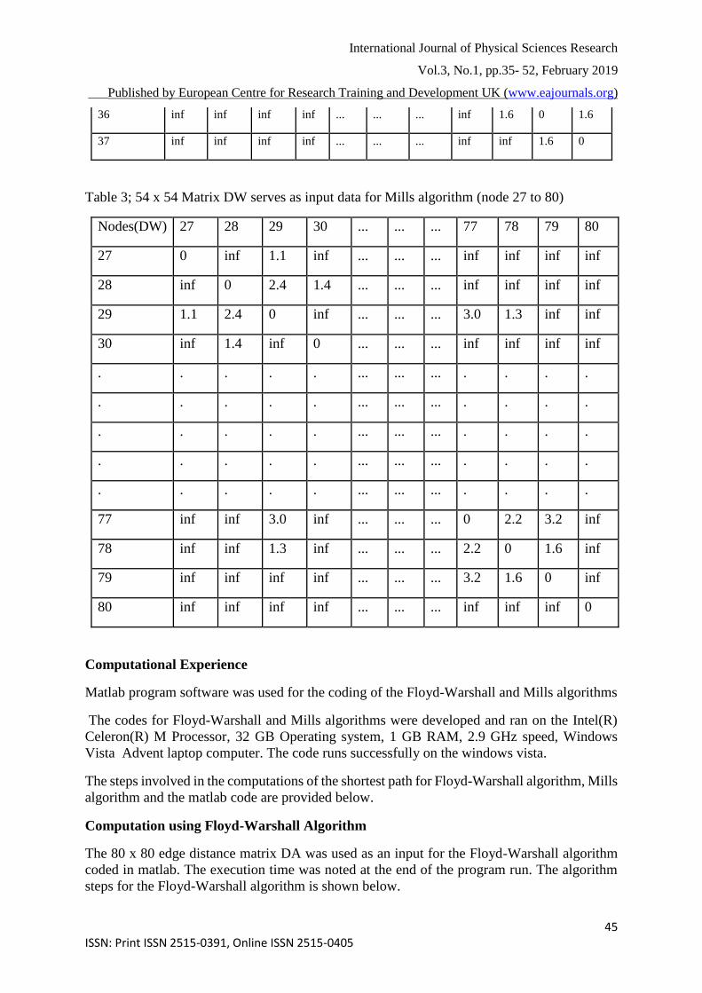
Table 3; 54 x 54 Matrix DW serves as input data for Mills algorithm (node 27 to 80)

Nodes(DW) 27 28 29 30 ... ... ... 77 78 79 80

27 0 inf 1.1 inf ... ... ... inf inf inf inf

28 inf 0 2.4 1.4 ... ... ... inf inf inf inf

29 1.1 2.4 0 inf ... ... ... 3.0 1.3 inf inf

30 inf 1.4 inf 0 ... ... ... inf inf inf inf

. . . . . ... ... ... . . . .

. . . . . ... ... ... . . . .

. . . . . ... ... ... . . . .

. . . . . ... ... ... . . . .

. . . . . ... ... ... . . . .

77 inf inf 3.0 inf ... ... ... 0 2.2 3.2 inf

78 inf inf 1.3 inf ... ... ... 2.2 0 1.6 inf

79 inf inf inf inf ... ... ... 3.2 1.6 0 inf

80 inf inf inf inf ... ... ... inf inf inf 0

Computational Experience

Matlab program software was used for the coding of the Floyd-Warshall and Mills algorithms

The codes for Floyd-Warshall and Mills algorithms were developed and ran on the Intel(R)

Celeron(R) M Processor, 32 GB Operating system, 1 GB RAM, 2.9 GHz speed, Windows

Vista Advent laptop computer. The code runs successfully on the windows vista.

The steps involved in the computations of the shortest path for Floyd-Warshall algorithm, Mills

algorithm and the matlab code are provided below.

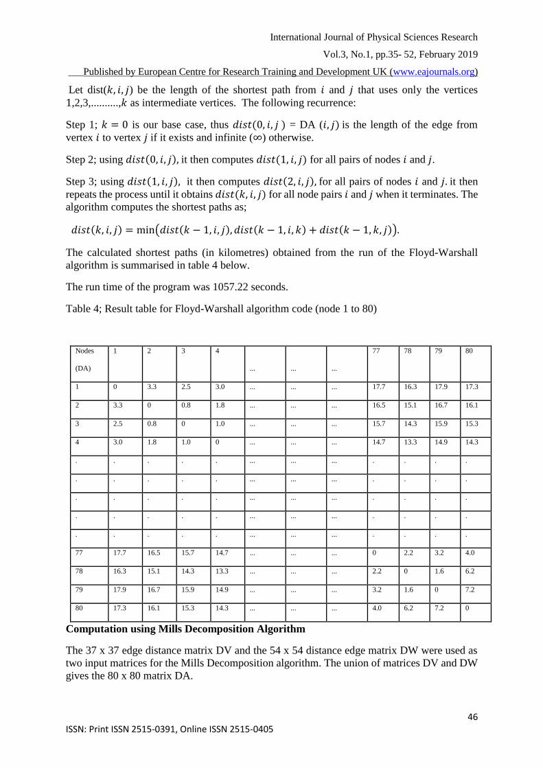
Computation using Floyd-Warshall Algorithm

The 80 x 80 edge distance matrix DA was used as an input for the Floyd-Warshall algorithm

coded in matlab. The execution time was noted at the end of the program run. The algorithm

steps for the Floyd-Warshall algorithm is shown below.






Let dist(𝑘, 𝑖, 𝑗) be the length of the shortest path from 𝑖 and 𝑗 that uses only the vertices

1,2,3,..........,𝑘 as intermediate vertices. The following recurrence:

Step 1; 𝑘 = 0 is our base case, thus 𝑑𝑖𝑠𝑡(0, 𝑖, 𝑗 ) = DA (𝑖, 𝑗) is the length of the edge from

vertex 𝑖 to vertex 𝑗 if it exists and infinite (∞) otherwise.

Step 2; using 𝑑𝑖𝑠𝑡(0, 𝑖, 𝑗), it then computes 𝑑𝑖𝑠𝑡(1, 𝑖, 𝑗) for all pairs of nodes 𝑖 and 𝑗.

Step 3; using 𝑑𝑖𝑠𝑡(1, 𝑖, 𝑗), it then computes 𝑑𝑖𝑠𝑡(2, 𝑖, 𝑗), for all pairs of nodes 𝑖 and 𝑗. it then

repeats the process until it obtains 𝑑𝑖𝑠𝑡(𝑘, 𝑖, 𝑗) for all node pairs 𝑖 and 𝑗 when it terminates. The

algorithm computes the shortest paths as;

𝑑𝑖𝑠𝑡(𝑘, 𝑖, 𝑗) = min(𝑑𝑖𝑠𝑡(𝑘 − 1, 𝑖, 𝑗), 𝑑𝑖𝑠𝑡(𝑘 − 1, 𝑖, 𝑘) + 𝑑𝑖𝑠𝑡(𝑘 − 1, 𝑘, 𝑗)).

The calculated shortest paths (in kilometres) obtained from the run of the Floyd-Warshall

algorithm is summarised in table 4 below.

The run time of the program was 1057.22 seconds.

Table 4; Result table for Floyd-Warshall algorithm code (node 1 to 80)

Nodes

(DA)

1 2 3 4

... ... ...

77 78 79 80

1 0 3.3 2.5 3.0 ... ... ... 17.7 16.3 17.9 17.3

2 3.3 0 0.8 1.8 ... ... ... 16.5 15.1 16.7 16.1

3 2.5 0.8 0 1.0 ... ... ... 15.7 14.3 15.9 15.3

4 3.0 1.8 1.0 0 ... ... ... 14.7 13.3 14.9 14.3

. . . . . ... ... ... . . . .

. . . . . ... ... ... . . . .

. . . . . ... ... ... . . . .

. . . . . ... ... ... . . . .

. . . . . ... ... ... . . . .

77 17.7 16.5 15.7 14.7 ... ... ... 0 2.2 3.2 4.0

78 16.3 15.1 14.3 13.3 ... ... ... 2.2 0 1.6 6.2

79 17.9 16.7 15.9 14.9 ... ... ... 3.2 1.6 0 7.2

80 17.3 16.1 15.3 14.3 ... ... ... 4.0 6.2 7.2 0

Computation using Mills Decomposition Algorithm

The 37 x 37 edge distance matrix DV and the 54 x 54 distance edge matrix DW were used as

two input matrices for the Mills Decomposition algorithm. The union of matrices DV and DW

gives the 80 x 80 matrix DA.






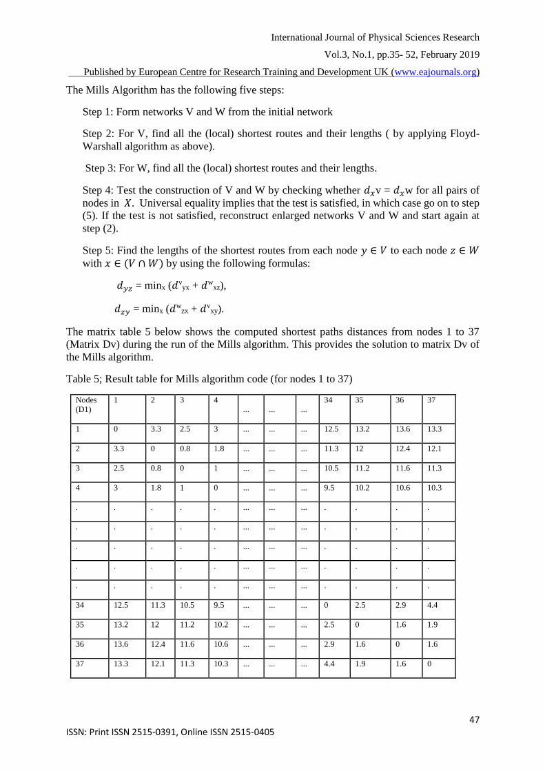
The Mills Algorithm has the following five steps:

Step 1: Form networks V and W from the initial network

Step 2: For V, find all the (local) shortest routes and their lengths ( by applying Floyd-

Warshall algorithm as above).

Step 3: For W, find all the (local) shortest routes and their lengths.

Step 4: Test the construction of V and W by checking whether 𝑑𝑥v = 𝑑𝑥w for all pairs of

nodes in 𝑋. Universal equality implies that the test is satisfied, in which case go on to step

(5). If the test is not satisfied, reconstruct enlarged networks V and W and start again at

step (2).

Step 5: Find the lengths of the shortest routes from each node 𝑦 ∈ 𝑉 to each node 𝑧 ∈ 𝑊

with 𝑥 ∈ (𝑉 ∩ 𝑊) by using the following formulas:

𝑑𝑦𝑧 = minx (𝑑vyx + 𝑑w

xz),

𝑑𝑧𝑦 = minx (𝑑wzx + 𝑑v

xy).

The matrix table 5 below shows the computed shortest paths distances from nodes 1 to 37

(Matrix Dv) during the run of the Mills algorithm. This provides the solution to matrix Dv of

the Mills algorithm.

Table 5; Result table for Mills algorithm code (for nodes 1 to 37)

Nodes

(D1)

1 2 3 4

... ... ...

34 35 36 37

1 0 3.3 2.5 3 ... ... ... 12.5 13.2 13.6 13.3

2 3.3 0 0.8 1.8 ... ... ... 11.3 12 12.4 12.1

3 2.5 0.8 0 1 ... ... ... 10.5 11.2 11.6 11.3

4 3 1.8 1 0 ... ... ... 9.5 10.2 10.6 10.3

. . . . . ... ... ... . . . .

. . . . . ... ... ... . . . .

. . . . . ... ... ... . . . .

. . . . . ... ... ... . . . .

. . . . . ... ... ... . . . .

34 12.5 11.3 10.5 9.5 ... ... ... 0 2.5 2.9 4.4

35 13.2 12 11.2 10.2 ... ... ... 2.5 0 1.6 1.9

36 13.6 12.4 11.6 10.6 ... ... ... 2.9 1.6 0 1.6

37 13.3 12.1 11.3 10.3 ... ... ... 4.4 1.9 1.6 0






The summary results table 6 below gives the computed shortest paths for the second matrix

(Dw) of the Mills algorithm. This shows the shortest paths from node 27 to 80 (Matrix Dw)

during the run of the Mills algorithm.

Table 6; Results table for Mills algorithm code (node 27 to 80)

Nodes

(R1)

27 28 29 30

... ... ...

77 78 79 80

27 0 3.5 1.1 4.9 ... ... ... 4.1 2.4 4.0 8.1

28 3.5 0 2.4 1.4 ... ... ... 5.4 3.7 5.3 5.7

29 1.1 2.4 0 3.8 ... ... ... 3.0 1.3 2.9 7.0

30 4.9 1.4 3.8 0 ... ... ... 5.6 5.1 6.7 5.2

. . . . . ... ... ... . . . .

. . . . . ... ... ... . . . .

. . . . . ... ... ... . . . .

. . . . . ... ... ... . . . .

. . . . . ... ... ... . . . .

77 4.1 5.4 3.0 5.6 ... ... ... 0 2.2 3.2 4.0

78 2.4 3.7 1.3 5.1 ... ... ... 2.2 0 1.6 6.2

79 4.0 5.3 2.9 6.7 ... ... ... 3.2 1.6 0 7.2

80 8.1 5.7 7.0 5.2 ... ... ... 4.0 6.2 7.2 0

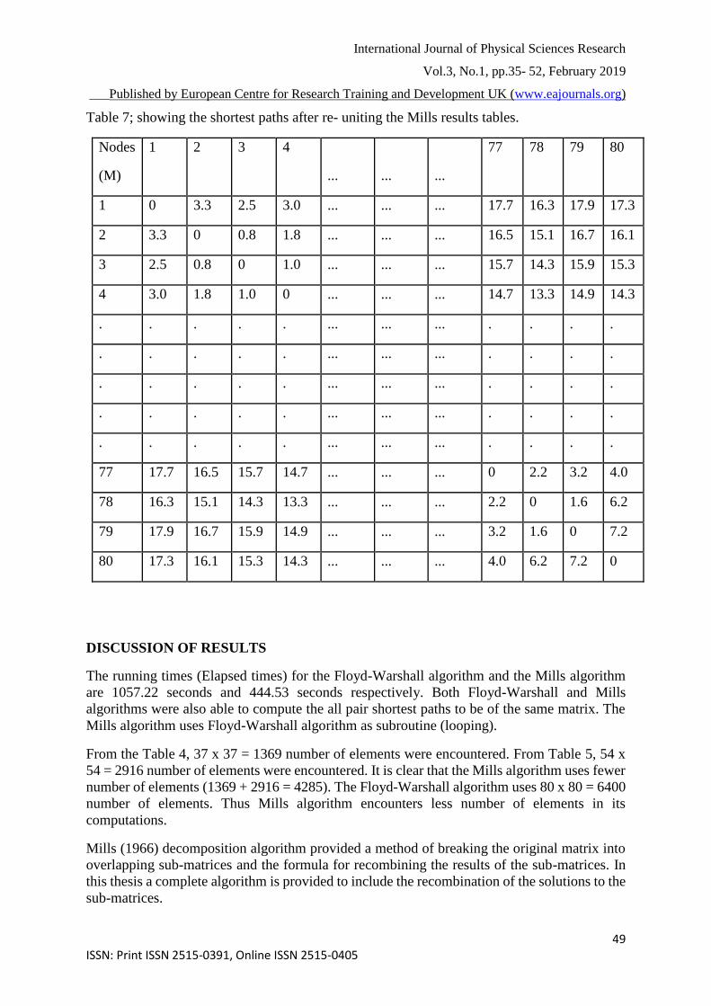
The summary results table 7 below provide the shortest paths after reuniting the results tables

5 and table 6. The final results obtained from the run of Mills algorithm was the same as that

of the Floyd-Warshall algorithm. The run time for Mills algorithm was 444.53 seconds.






Table 7; showing the shortest paths after reuniting the Mills results tables.

Nodes

(M)

1 2 3 4

... ... ...

77 78 79 80

1 0 3.3 2.5 3.0 ... ... ... 17.7 16.3 17.9 17.3

2 3.3 0 0.8 1.8 ... ... ... 16.5 15.1 16.7 16.1

3 2.5 0.8 0 1.0 ... ... ... 15.7 14.3 15.9 15.3

4 3.0 1.8 1.0 0 ... ... ... 14.7 13.3 14.9 14.3

. . . . . ... ... ... . . . .

. . . . . ... ... ... . . . .

. . . . . ... ... ... . . . .

. . . . . ... ... ... . . . .

. . . . . ... ... ... . . . .

77 17.7 16.5 15.7 14.7 ... ... ... 0 2.2 3.2 4.0

78 16.3 15.1 14.3 13.3 ... ... ... 2.2 0 1.6 6.2

79 17.9 16.7 15.9 14.9 ... ... ... 3.2 1.6 0 7.2

80 17.3 16.1 15.3 14.3 ... ... ... 4.0 6.2 7.2 0

DISCUSSION OF RESULTS

The running times (Elapsed times) for the Floyd-Warshall algorithm and the Mills algorithm

are 1057.22 seconds and 444.53 seconds respectively. Both Floyd-Warshall and Mills

algorithms were also able to compute the all pair shortest paths to be of the same matrix. The

Mills algorithm uses Floyd-Warshall algorithm as subroutine (looping).

From the Table 4, 37 x 37 = 1369 number of elements were encountered. From Table 5, 54 x

54 = 2916 number of elements were encountered. It is clear that the Mills algorithm uses fewer

number of elements (1369 + 2916 = 4285). The Floyd-Warshall algorithm uses 80 x 80 = 6400

number of elements. Thus Mills algorithm encounters less number of elements in its

computations.

Mills (1966) decomposition algorithm provided a method of breaking the original matrix into

overlapping sub-matrices and the formula for recombining the results of the sub-matrices. In

this thesis a complete algorithm is provided to include the recombination of the solutions to the

sub-matrices.






The algorithms also provide precedence table accompanying the calculated shortest paths for

navigation.

From the above results, it is more convenient and efficient in terms of time to use the Mills

decomposition algorithm when solving network problems with large number of nodes.

CONCLUSION

The Floyd-Warshall and Mills algorithms for solving all pairs shortest paths problem have been

successfully applied to the Sunyani Municipality road network. Matlab codes were written to

determine the running time for the two algorithms. When the network was solved using the

Floyd-Warshall algorithm the running time was 1057.22 seconds; when the network was solved

by the Mills algorithm the total running time was 444.53 seconds. The network was further

partitioned into two equal halves and the running time was 417.27 seconds. When the network

was partitioned into three equal parts the running time was found to be 51.81 seconds and four

partitions also gave the running time to be 24.94 seconds. This means as the number of

partitions increases, the running time also decreases. Base on the results of this study the

assertion made by Hu (1968) and Mills (1966) that the decomposition algorithm runs faster

than solving the whole network is confirmed.

RECOMMENDATIONS

Base on the study, the following recommendations are made.

This work should serve as basis for further research in shortest path.

Finally, since Sunyani Municipality was used as case study, the researcher recommend that the

Municipal Assembly, feeder and urban roads , contractors and others should make use of this

study and the project code in their operations; such as road constructions and expansion of

electricity in the Municipality.

REFERENCES

1. Algorithmist (2005). Floyd-Warshall Algorithm. GNU. http://www.algorithmist.com.

(Accessed on 22/12/2010)

2. Amponsah, S. K. and Darkwa, F. K. (2008). Lecture notes. Operations Research.

Kwame Nkrumah University of Science and Technology. Kumasi pp. 16 – 22.

3. Andreas, L. and Weintein, E. W. (2010). Graph algorithms with applications. Reese.

http//www.bruce-shapiro.com/math382/projects/reese. (Accessed on 14/02/2011)

4. Arendts, D. (2009). Vectorized Floyd-Warshall. file Exchange.

http://www.mathwork.com/matlabcentral/fileexchange. (Accessed on 21/01/2010).

5. Awasthi, A., lechevallier, Y., Parent, M. and Proth, J. M. (2007). ACM.

http/www.portal.acm.org/citation.cfm. (Accessed on 02/10/2010)


http://www.algorithmist.com/

http://www.mathwork.com/matlabcentral/fileexchange





6. Bellman, R. and Ford, H. (1958). On a Routing Problem in Quarterly of Applied

Mathematics. Vol. 16. No. 1. pp. 87-90.

7. Dijkstra, E. (1956). Dijskstra’s algorithm. Wikipedia.

http://en.wikipedia.org/wiki/Dijkstra’s_algorithm. (Accessed on 20/08/2010).

8. Dreyfus, S. E. (1968). An Appraisal of Some Shortest-Path Algorithms. Informs. Vol.

17. No.3. pp.395-412. http://www.jstor.org/stable/168375. (Accessed on 02/06/2010).

9. Erden, T. and Coskun M. Z. (2006). Analyzing shortest and fastest paths with GIS and

determing algorithm running time. ITU. http//www.spingerlink.com/index. (Accessed

on 15/09/2010).

10. Frederickson, G. N. (2001). Fast algorithms for shortest paths in planar graph, with

applications. ACM. http//www.portal.acm.org. (Accessed on 05/02/2011)

11. Hahn, B. and Valentine, D. T. (2007). Essential Matlab for Engineers and Scientists. 3rd

Edition. Elsevier. Oxford.

12. Hiller, F. S. and Lieberman, G. J. (2000). Advance Praise for Introduction to Operation

Research. 7th Edition. McGraw Hill. New York. pp. 5-43.

13. Hu, T. C. (1968). A Decomposition Algorithm for Shortest Paths in a Network.

Informs, Vol. 16. No.1. pp. 91-102. http://www.jstor.org/stable/168405. (Accessed on

02/06/2010).

14. Johnson, L. E. (2005). A Multiple Pairs Shortest Path Algorithm. Georgia Institute of

Technology. Atlanta. Georgia

15. Kleinschmith, L. (2010). Speed Up, your shortcut to productivity and success. German

Efficiency. Huamburg.

16. Lee, Y. (2007). Shortest Path in a Grid. A life on the web.

http//www.sougatasantra.wordpress.com. (Accessed on 17/01/2011)

17. Li, Y., Gen, M. and Ida, K. (1996). Solving fuzzy shortest path problems by neural

networks. Department of Industrial and Systems Engineering. Institute of Technology.

Ashikaga. Japan.

18. Mill, G. (1966). A Decomposition Algorithm for the Shortest-Route Problem. Informs.

Vol. 14 No.2. pp. 279-291. http://www.jstor.org/stble/168255. (Accessed on

02/06/2010).

19. Mohemmed, A. W. (2008). A new particle swarm optimization base for solving shortest

paths tree problem algorithm. Scholar. http://www.ieeexplore.ieee.org. (Accessed on

15/09/2010).

20. Mondal, S., Madhumangal, P. and Tapan, K. (2003). An Optimal Algorithm to Solve

the All-Pairs Shortest Paths Problem on Permutation Graphs. Department of Applied

Mathematics with Oenology and Computer Programming. Vidyasagar University.

Midnapore. India.

21. Mondou, J. F., Crainic, T. G., and Nguyen, S. (1991). Shortest Path Algorithms: A

Computational Study with the C Programming Language. Vol. 18. 767-786.

22. Noon, C. E., Daly, M. and Zhan. F. B. (1996). Beyond Assessment of Resources:

Procurement of Woody Biomass Fuels. Nashville University. Tennessee. pp.565-569.

23. Pires M. G. (2008). Solving shortest path problem using Hopfield Networks and

Genetic algorithm. IEEE xplore. http://www.ieeexplore.ieee.org. (Accessed on

15/09/2010)

24. Rabbani, S. (2008). Maximum mutual links-Kth Shortest Path Restoration Protocol.

ECE. http//www.ece.queensu.ca/people. (Accessed on 15/09/2010).

25. Roy, B. (1959). Floyd-Warshall Algorithm. Wikipedia.

http//en.wikipedia.org/wik/Floyd-warshall. (Accessed on 22/12/2010).


http://en.wikipedia.org/wiki/Dijkstra's_algorithm

http://www.jstor.org/stable/168375

http://www.jstor.org/stable/168405

http://www.jstor.org/stble/168255





26. Sung-Chul, H., Franchetti, F. and Puschel, M.(2006). Program Generation for the All-

Pairs Shortest Path Problem. Electrical and Computer Engineering. Carnegie Mellon

University. Pittsburgh.

27. Wang, Z. (1990). A Shortest Augmenting Path Algorithm for the Semi-Assignment

Problem. Southern Methodist University. Dallas. Texas.

28. Warshall, S.(1962). Floyd-Warshall algorithm. Wikipedia.

http://en.wikipedia.org/wiki/Floyd-Warshall_algorithm. (Accessed on 15/9/2010).

29. Wu, Q. (1974). Using K-Shortest paths algorithm. http://www.ist.psu.edu/viewdoc.

(Accessed on 15/09/2010)

30. Xiao, X. (2009). Hierarchic Genetic Algorithm for Designated Multi-nodes Routing.

Second international symposium. Scholar. http://www.computer.org. (Accessed on

15/09/2010)

31. Yen, J. Y. (1970). On Hu’s Decomposition Algorithm for shortest Paths in a Network.

University of Santa Clara. California.

32. Zhan, F. B. (1996).Three Fastest Shortest Path Algorithms on Real Road Networks:

Data Structures and Procedures. Department of Geography and Planning. Southwest

Texas State University. San Marcos.

33. Zuubier, E. (2004). Solving All Pairs Shortest Path Problem. Bing.

http://www.mathb.com.uwe. (Accessed on 21/01/2011).


http://www.ist.psu.edu/viewdoc

http://www.computer.org/

http://www.mathb.com.uwe/

COMPARISON OF FLOYD-WARSHALL AND MILLS ALGORITHMS … · the Floyd-Warshall and Mills are 1057.22...

Documents

Transcript of COMPARISON OF FLOYD-WARSHALL AND MILLS ALGORITHMS … · the Floyd-Warshall and Mills are 1057.22...