ii

Civil Engineering Studies Transportation Engineering Series No. 113 Traffic Operations Lab Series No. 1

UILU-ENG-2001-2005

ISSN-0917-9191

Comparison of Delays from HCM, Synchro, PASSER II,

PASSER IV and CORSIM for an Urban Arterial

By Rahim F. Benekohal Yoassry M. Elzohairy Joshua E. Saak A study conducted by the Traffic Operations Laboratory Department of Civil and Environmental Engineering University of Illinois at Urbana-Champaign Urbana, Illinois Prepared for The Illinois Department of Transportation August 2001

ii

Technical Report Documentation Page 1.. Report No,

FHWA-IL/UI-TOL-1 2. Government Accession No.

3. Recipient's Catalog No

5. Report Date

August 30, 2001 6. Performing Organization Code

4. Title and Subtitle

Comparison of Delays from HCM, Synchro, PASSER II, PASSER IV and CORSIM for an Urban Arterial

7.Author(s)

Rahim F. Benekohal, Yoassry M. Elzohairy, and Joshua Saak

8. Performing Organization Report No.

UILU-ENG-2001-2005

9. Performing Organization Name and Address

10. Work Unit (TRAIS) 11. Contract or Grant No.

Department of Civil and Environmental EngineeringUniversity of Illinois at Urbana-Champaign 205 N. Mathews Ave. Urbana, Illinois 6180

13. Type of Report and Period Covered

Project Report 1999-2001

12. Sponsoring Agency Name and Address

The Illinois Department of Transportation

14. Sponsoring Agency Code

15. Supplementary

16. Abstract This study compared control delays computed by HCM (using HCS software), Synchro, PASSER II, PASSER IV, and CORSIM for an urban arterial. Base and optimized conditions were studied. In the base condition, the existing signal settings and traffic volumes were modeled in HCS and Synchro under three scenarios: actuated-coordinated, actuated-uncoordinated and pre-timed traffic controller. For the base condition, delays from HCM shouldn’t be directly compared to Synchro unless the precautions discussed in this report are taken. For pre-timed and actuated signals when simultaneous phases exist and one terminates ahead of the others, the results of HCM and Synchro are not comparable. For pre-timed and actuated signals where the phases terminate simultaneously, the condition analyzed won’t be comparable unless the precautions are taken. Once these precautions were taken, control delays from Synchro and HCM were not significantly different for only pre-timed uncoordinated signals. For actuated-uncoordinated and for actuated-coordinated, the software are modeling different conditions. For the optimized condition, the software optimized signal settings for actuated coordinated signal controllers and calculated the delays. The delays for optimized conditions from PASSER II and PASSER IV were not significantly different than the delays for the base conditions. However, the delays from Synchro for optimized conditions were significantly lower than the delays for the base conditions. CORSIM was used to verify whether the optimized signal settings would produce lower delay if implemented in the field. The results indicated that delays for optimized conditions would not be significantly lower than the delays for the base conditions, and the lower delays given by Synchro for the optimized conditions could not be verified.

17. Key Words Intersection Delay, Delay Models, Highway Capacity Manual (HCM), HCS, Synchro, PASSER, CORSIM, Simulation Models, Urban Arterial

18. Distribution Statement

19. Security Classif. (of this report)

Unclassified

20. Security Classif. (of this page)

Unclassified

21. No. of Pages

48

22. Price

`Form DOT F 1700.7 (8-72) Reproduction of completed page authorized

iii

Acknowledgment and Disclaimer

This study was conducted by the Traffic Operations Laboratory (TOL) at the University of Illinois at Urbana-Champaign. The Illinois Department of Transportation sponsored the study. The contents of this report reflect the views of the authors who are responsible for the facts and accuracy of the data presented herein. The contents do not necessarily reflect the official views or policies of the Illinois Department of Transportation. This report does not constitute a standard, specification, or regulation.

iv

TABLE OF CONTENTS

TABLE OF CONTENTS ........................................................................................................................... IV

INTRODUCTION ........................................................................................................................................ 1

STUDY OBJECTIVES ................................................................................................................................ 3

OVERVIEW OF THE SOFTWARE USED IN THIS STUDY................................................................ 3

HIGHWAY CAPACITY SOFTWARE – 1997 (HCS-97) ................................................................................... 3 SYNCHRO.................................................................................................................................................... 5 PASSER II-90............................................................................................................................................ 5 PASSER IV-96 .......................................................................................................................................... 5 CORSIM.................................................................................................................................................... 6

STUDY APPROACH................................................................................................................................... 6

DELAY CALCULATIONS .............................................................................................................................. 7 Delay Calculations in HCS ................................................................................................................... 7 Delay Calculations in Synchro.............................................................................................................. 8 Delay Calculations in PASSER............................................................................................................. 9 Delay Calculation in CORSIM............................................................................................................ 10

LOS DETERMINATION.............................................................................................................................. 11 BASE CONDITION...................................................................................................................................... 12 OPTIMIZED CONDITION............................................................................................................................. 13 SIMULATION OF OPTIMIZED CONDITION IN CORSIM................................................................................ 13

Methods of handling overlapping phase in CORSIM.......................................................................... 14

STATISTICAL ANALYSIS OF RESULTS............................................................................................. 16

COMPARISONS OF THE RESULTS ..................................................................................................... 17

BASE CONDITION...................................................................................................................................... 17 OPTIMIZED CONDITION............................................................................................................................. 19 OPTIMIZED CONDITIONS SIMULATED IN CORSIM.................................................................................... 21

ISSUES IN COMPARING HCM AND SYNCHRO ............................................................................... 26

CONCLUSIONS AND RECOMMENDATIONS.................................................................................... 27

APPENDIX A: BASE CONDITION......................................................................................................... 33

APPENDIX B: SUMMARIZED DATA, OPTIMIZED CONDITION.................................................. 43

APPENDIX C: SUMMARIZED DATA, CORSIM OPTIMIZED CONDITION ................................ 45

REFERENCES ........................................................................................................................................... 48

1

INTRODUCTION

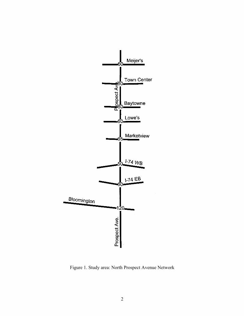
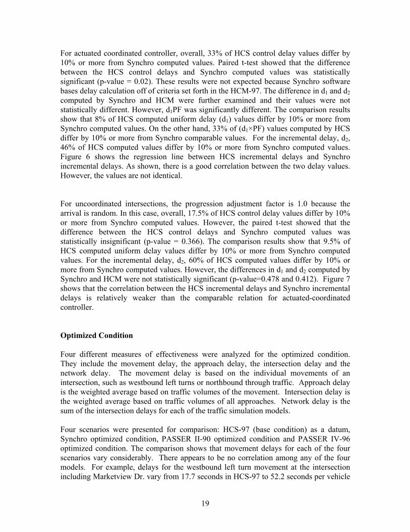
Improving traffic signal timing and coordination is one of the most widely used strategies for relieving congestion and enhancing mobility. Illinois Department of Transportation (IDOT) annually retains consultants to review traffic signal control systems through SCAT (signal coordination and timing) program. The consultants usually use one of the popular traffic software packages for the evaluation and may suggest modifications to signal settings to minimize network delay. This study compares a number of traffic software packages, including Highway Capacity Software (HCS-97), PASSER II-90, PASSER IV-96, Synchro (Ver. 3.2 and Ver. 4.0), and CORSIM. The objective of the comparison is to determine which software quantifies delays more accurately. It also compares how each software optimizes the signal setting to reduce delays. Finally, the study answers the question whether the claim of delay reduction does materialize when the optimized signal settings are implemented in field. Simulation models are useful tools that enable the traffic engineer to model real-life traffic conditions without disrupting everyday operations. Simulation models are also a low cost alternative to actual field implementation of traffic improvement measures. Theoretical improvements can be modeled before they are introduced in highway applications to obtain the best course of action in a given scenario. In a sense, they enable the traffic engineer to improve driving conditions by a trial and error method that will reduce delay to a minimum. One of the issues that can arise from using traffic modeling packages is how well does the package model a given traffic condition. Some users may prefer a specific modeling program in all cases, others may use a different program because it has a user-friendly interface. In either case, the results obtained from the simulation may not be what actually occurs in the field. It may be true that software previously accepted as able to provide accurate modeling may in truth not be applicable to a particular traffic situation. The purpose of this study is to compare various traffic modeling programs using an actual network with existing peak hour traffic. The programs are capable of performing different functions, and our objective is to provide guidance on which simulation is applicable to a given situation. The network modeled is the North Prospect Avenue arterial in Champaign, Illinois from Bloomington Road in the south to Meijer Drive in the north. Development in the North Prospect Avenue area in Champaign has increased substantially in the past decade. Much of the development has consisted of retail stores, restaurants, and large discount superstores. This arterial was chosen due to the proximity of numerous signals, relatively heavy traffic conditions, and lack of access and egress to Prospect Avenue without encountering a traffic signal. A map of the network configuration is shown in Figure 1.

2

Figure 1. Study area: North Prospect Avenue Network

3

STUDY OBJECTIVES The objectives of this study include: 1. Compare the output from the software in the base condition (using the existing

signal timings of the peak traffic period) to each other using predetermined measures of effectiveness (MOEs).

2. Compare the output from the software in the optimized condition to each other.

In the optimized condition, the program decides a signal timing that it thinks will minimize delay and maximize flow.

3. Evaluate the optimized solutions obtained from Synchro, PASSER II and

PASSER IV using CORSIM. For this objective, each optimized set of timings will be input into the same traffic simulator (CORSIM) and results will be compared.

4. Discuss items of confusion that may result from the use of the programs and

discrepancies between what the software can and cannot do. 5. Provide a guideline on the selection of appropriate signal coordination models. OVERVIEW OF THE SOFTWARE USED IN THIS STUDY It is important to elaborate on the traffic models used in this study in relation to what each of them are capable of. It is also important to note what each simulation is not equipped to model, which is important when comparing simulated results to actual field conditions. The following will expound on the abilities of the software we used in this study and help to clarify some possible items of confusion regarding situations applicable to each. Table 1 provides a summary of key features of each software. Highway Capacity Software – 1997 (HCS-97) The Highway Capacity Manual (HCM), from which HCS-97 is derived, is considered the “bible” of roadway capacity analysis. The first HCM was published in 1950 as a joint venture between the Highway Research Board’s Committee on Highway Capacity and the Bureau of Public Roads. Materials in the HCM are a collection of techniques for estimating capacity and level of service for many transportation facilities and modes. These techniques were developed by funded research and research results by the Committee on Highway Capacity and Quality of Service (1). It has been updated several

4

times since, most recently in 2000. In 1985, computer software was created as an extension of the manual (HCS-85). The Windows™ based software that was used for this study is based directly off of the HCM-97 update. It incorporates the capacity and level of service calculations present in the 1997 HCM. It does not have the ability to automatically determine optimal phase plans. The 2000 Highway Capacity Manual (HCM 2000) basically uses the same procedure that was in HCM 97.

DO

S ba

sed

Win

dow

s ba

sed

Mul

tiple

Arte

rials

Ba

sed

off H

CM

O

ptim

izes

Tim

ings

M

axim

izes

Ban

dwid

th

Exis

ting

Phas

e Pl

an

Gra

phic

al

Rep

rese

ntat

ion

Mod

els

Excl

usiv

e LT

La

neM

odel

s Ex

clus

ive

RT

Lane

Rep

orts

Sto

pped

del

ay

Rep

orts

Con

trol

dela

y C

apac

ity A

naly

sis

Mul

tiple

C

ycle

le

ngth

Ba

ndw

idth

Dia

gram

HCS-97 X X X X X X X

Synchro 3.2 X X X X X X X X X X X

Synchro 4.0 X X X X X X X X X X X X

PASSER II-90 X X X X X X X

PASSER IV-96 X X X X X X X X X

CORSIM 4.0 X X X X X X X X

Table 1 - Capabilities and Characteristics of Traffic Software

5

Synchro Synchro, developed by Trafficware Inc., is a software package able to model and optimize traffic signal timings. Synchro Ver.3.2 implements the method of the HCM-94, Chapter 9, signalized intersections. Synchro 4 implements the new methods of the 1997 Highway Capacity Manual's chapter on signals. HCM 1997 Chapter 9, includes methods for analyzing actuated and congested signals. The delays used by the new HCM are "Control Delay" and are 30% higher than the "Stopped Delay" used in HCM 1994 and Synchro 3.2. Synchro is Windows™ based and can be used for intersection capacity and/or timing optimization. Synchro also has the ability to compute optimum intersection timings for intersection offsets as well as cycle lengths and phase splits. Unlike HCS-97, Synchro can optimize phase splits, cycle lengths and timing offsets. Synchro uses an optimization process that minimizes delay for a given intersection, as opposed to arterial software (PASSER II-90) that maximizes the ability for a vehicle to pass through a given network with minimal stopping. Like HCS, Synchro has the ability to model actuated signals. The software needs additional information from the user in order to analyze an actuated network. Detector location, signal timings, and observed range of green times are all necessary items that need to be included for an actuated network. It also creates time-space diagrams to show vehicle progression through a network, as do PASSER II-90, and PASSER IV-96. PASSER II-90 The Progression Analysis and Signal System Evaluation Routine (PASSER II-90) is a traffic software program that is used to optimize and coordinate signalized arterial streets. It was developed by the Texas Transportation Institute in the early 1980s. It is a DOS based program that has the ability to handle left turns as protected, permitted, or a combination of left turn phases. In addition, PASSER II-90 can select multiple phase plans, one-way streets, vary cycle length and maximize arterial progression. It has the capability to analyze one arterial street at a time. PASSER IV-96 PASSER IV-96 was developed by the Texas Transportation Institute in the early 1990s and is based on the MAXBAND program. It is a DOS based program used to optimize a network of traffic signals based on maximum bandwidth. Maximum bandwidth is obtained by maximizing the time period that a car can potentially pass through a given network with minimal stopping at signalized intersections. It is able to optimize signal timings for arterials as well as closed-loop networks, such as a downtown area or central

6

business district (CBD). Unlike PASSER II-90, PASSER IV-96 can handle multiple arterials as well as one-way and two-way arterials in a network. CORSIM CORSIM, developed by Federal Highway Administration, is a simulation program that is part of the Traffic Software Integrated System (TSIS). It is a Windows™ based program that can be used in conjunction with other programs that were created by outside parties to facilitate its use. TSIS is an integrated traffic simulation model that can be used to input traffic data, provide a common user interface, perform microscopic simulation, and animate a given network. ITRAF, part of the TSIS software, is a program used to input data in a CORSIM file. TRAFVU is also part of the TSIS package; it is able to provide a graphical representation of a CORSIM network that can give the user an idea of how given phase plans would work in real world conditions. CORSIM performs the simulation and returns to the user the efficiency of the network in predetermined MOEs.

CORSIM is able to simulate existing or proposed conditions on a network, but is unable to optimize phase plans. Very large networks can be modeled. It is capable of modeling actuated signals and offsets. CORSIM is a rather complicated program that can take time to debug. Unlike other simulations, CORSIM models varied driver behavior and figures different driver characteristics into each separate run. As a result, numerous runs may need to be performed to obtain an accurate representation of a network.

STUDY APPROACH Field data was collected in the summer of 1997 for the North Prospect Avenue network. The peak hour period was assumed to be from 3pm to 5pm. Traffic data from the heaviest traveled hour was used for this study. The same traffic volumes were used for all software. Two conditions were evaluated in this study: Base condition and Optimized condition. In the base condition, the existing signal timing and traffic data collected from 8 intersections of North Prospect Ave were used as input to the following models to compute MOEs and LOS:

- HCS-97 - Synchro Ver. 4.0 - CORSIM

7

In the optimized condition, the network was first optimized using - Synchro Ver. 3.2 - PASSER-II - PASSER-IV

The optimized signal settings produced by each of the three software were used as input into CORSIM. For each setting, we ran CORSIM fifteen times; 5 runs (5 random seeds) for each of the three options outlined later under the paragraph titled “Methods of handling overlapping phase in CORSIM.” The MOEs used in this study include average control delay per approach, average control delay per intersection, and level of service (LOS). Average control delay per approach is the amount of time the average vehicle spends at an intersection. It includes stopped delay, acceleration and deceleration delay. Average control delay per intersection is the weighted average of the control delay for each individual approach at an intersection based on the volume of traffic for each approach. LOS is a measure of delay designated by a letter A through F. LOS A represents nearly ideal traffic conditions while LOS F represents breakdown conditions and large delays. LOS criteria are based off of the Highway Capacity Manual (HCM) 1997. Delay Calculations

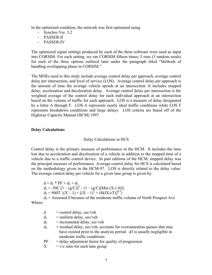
Delay Calculations in HCS Control delay is the primary measure of performance in the HCM. It includes the time lost due to acceleration and deceleration of a vehicle in addition to the stopped time of a vehicle due to a traffic control device. In past editions of the HCM, stopped delay was the principal measure of performance. Average control delay for HCS is calculated based on the methodology given in the HCM-97. LOS is directly related to the delay value. The average control delay per vehicle for a given lane group is given by: d = d1 * PF + d2 + d3

d1 = .50C [1 – (g/C)]2 / {1 – (g/C)[Min (X,1.0)]} d2 = 900T {(X – 1) + [(X – 1)2 + (8kIX/cT)]0.5} d3 = Assumed 0 because of the moderate traffic volume of North Prospect Ave Where: d = control delay, sec/veh d1 = uniform delay, sec/veh d2 = incremental delay, sec/veh d3 = residual delay, sec/veh, accounts for oversaturation queues that may

have existed prior to the analysis period. d3 is usually negligible in moderate traffic conditions.

PF = delay adjustment factor for quality of progression X = v/c ratio for each lane group

8

C = cycle length, sec T = length of analysis period, hours

k = incremental delay factor, dependant on control settings I = upstream filtering/metering adjustment factor c = capacity of lane group, vph

g = effective green time for lane group, sec Qb = initial queue at the start of period T,veh, t = duration of unmet demand in T, h, and u = delay parameter. Approach delay is computed as the weighted average of the individual lane groups. Approach delay is calculated as:

dA = Σ(di * vi) / Σ(vi) Where: dA = average delay per vehicle on the approach, sec/veh dI = average delay per vehicle on lane group i, sec/veh vi = adjusted flow for lane group i, vph The adjusted flow considers the percentage of heavy vehicles in the traffic stream as well as the peak hour factor (PHF) for each lane group. Intersection delay is computed in a similar fashion to approach delay. Instead of individual lane groups, a weighted average is used with the approach volumes and delays. Intersection delay is calculated as:

dI = Σ(dA * vA) / Σ(vA) Where: dI = average delay per vehicle on the intersection, sec/veh dA = average delay per vehicle for approach A, sec/veh vA = adjusted flow for approach A, vph

Delay Calculations in Synchro Synchro uses similar methodology in calculating intersection delay. Both versions used in this study (Ver. 3.2 and Ver 4.0) allows the user to choose which delay method he/she prefers to use. The two methods used in Synchro are Webster’s formula and Percentile delay method. In this study, we selected Webster’s formula, which is comparable to HCM delay. What Synchro calls Webster’s formula is the delay model in 1994 HCM. Synchro actually uses the HCM delay model and not the Webster’s formula that is found in literature. The 1994 HCM formula is defined as

9

d = d1 * PF + d2

Where: d = stopped delay (sec/veh) d1 = uniform delay (sec/veh) d2 = incremental delay (sec/veh) PF = delay adjustment factor for quality of progression To convert stopped delay to control delay, multiply stopped delay by 1.3.

Delay Calculations in PASSER PASSER II-90 and PASSER IV-96 use a slightly modified version of the HCM delay equation. The equation used is:

D = dU + dRS D is defined as the approach delay while dU is the uniform delay component and dRS is the random plus saturated delay. All delays are measured in sec/veh. The equations for uniform and random plus saturated delay are as follows: dU = [CVr * (1 – g/C)2] / [2V * {1 + Vr / (S – Vg)] Where: C = cycle time, sec g = effective green time, sec V = volume, veh/sec Vr, Vg = volume arriving on red and green, respectively, veh/sec S = saturation flow rate, veh/hr green time And: dRS = 225 * X2 * [(X – 1) + {(X – 1)2 + (16X / c)}0.5] Where: X = degree of saturation, or v/c ratio c = capacity, veh/hr The uniform delay component is the same used in Webster’s uniform delay model adopted in the HCM. The equation, however, has been modified to account for the progression effect on through movements. The difference in delay calculations is that

10

PASSER and HCS-97 predict approach delay while Synchro Ver 3.2 and HCS 94 only reports stopped delay. The difference is a factor of 1.3 for both terms.

Delay Calculation in CORSIM The CORSIM statistics provide a large number of variables for network analysis purposes. The table itself can be very confusing, due to the large amount of information that is presented. There are two parts to the output, the link-specific statistics (displayed one link per line) and the network wide statistics (displayed at the bottom of the sheet). Since this paper is concerned with approach and intersection delays, the link-specific statistics were used, most notably the delay time for each link on the network. Delay time is defined as the average delay on a link by a single vehicle. CORSIM calculates delay in a different manner than other simulation models. At any given time during a simulation run, there exist a specific number of vehicles on a road segment. The number of vehicles is specified by the input parameters. CORSIM can calculate the average delay for a vehicle on a given link because of the microscopic nature of the simulation. Microscopic analysis is best thought of as the ability to see each vehicle as an individual entity, as opposed to macroscopic simulation that only sees traffic flow as a stream of vehicles. The default value is a simulation time of 15 minutes, which is what was used in this case. For each link, delay time per vehicle in a network is calculated by CORSIM in the following manner (2): Delay time = Σ (T TL) – (Σ (VT) * L L) / FFS Σ (VT) Where: TTL = Total link travel time, veh-min VT = Completed vehicle trips LL = Link length, feet FFS = Free flow speed, mph Total link travel time – CORSIM accumulates link travel time only after a vehicle is released from the link. Travel time for vehicles still on that link are collected and added on to this figure. Completed vehicle trips – This is the number of vehicles discharged from the link since the beginning of the simulation. Trips are expressed in full trips, while partial trips are converted to full trips as appropriate. Partial trips are calculated from the number of vehicles still on the link at the beginning and the end of each simulation period.

11

Link length – It is defined to begin at the stop line and include the distance across an intersection at the beginning of each link. The intersection width of each node pair is subtracted for every vehicle entering the link by a right-turn maneuver, as these vehicles travel a shorter distance than left or through movements. Free flow speed – This is the speed that vehicles are supposed to travel under free flow conditions. It is usually near the speed limit for a given network. LOS Determination Due to the differences in the release dates of the software used, LOS varies slightly for delay values obtained through various trials. The most recent criteria for LOS were used, which is included in the HCM-97. LOS for signalized intersections is defined to represent reasonable ranges in control delay. LOS A details traffic flow through an intersection with a very low control delay, up to 10 sec/veh. Many vehicles may not even stop at all and short cycle lengths may contribute to low delay values. LOS B details traffic flow through an intersection with a control delay greater than 10 and up to 20 sec/veh. This usually occurs with good progression and short cycle length. LOS C details traffic flow through an intersection with a control delay greater than 20 and up to 35 sec/veh. Higher delays may occur from adequate progression or longer cycle lengths. The number of stopping vehicles is significant, but many still pass through the intersection without stopping. LOS D details traffic flow through an intersection with a control delay greater than 35 and up to 55 sec/veh. The influence of congestion becomes more noticeable at LOS D. Long cycle lengths, poor progression, or high v/c rations may result in the longer delays. Cycle failures are noticeable. LOS E details traffic flow through an intersection with a control delay greater than 55 and up to 80 sec/veh. LOS E usually indicates bad progression, long cycle lengths, or high v/c ratios. Cycle failures are frequent occurrences. LOS F details traffic flow through an intersection with a control delay greater than 80 sec/veh. This is usually considered to be unacceptable for most drivers. It often occurs with oversaturation, when arrival rates are greater than the capacity of the individual lane groups.

12

Base Condition Since North Prospect arterial has actuated-coordinated traffic control devices, the peak hour traffic volumes were modeled under this condition in Synchro 4. Synchro calculates delay based on actuated green times, not the maximum green times. Therefore, the input files for each of the eight intersections were exported from Synchro to the HCS-97 so that they will have the actuated green times. In addition, we modeled the network under actuated-uncoordinated and fixed-time for the peak hour traffic conditions. This enabled us to cover the different possible scenarios for controller types that may have been used in a similar network. For the North Prospect network, cycle length was not the same for every intersection. Therefore, PASSER II-90 and PASSER IV-96 were excluded from the comparison in the base condition because they are not able to simulate existing conditions for a network with intersections that have multiple cycle lengths. HCS-97 has the ability to calculate delay for an intersection based on given traffic volumes and existing phase timings. HCS-97 returns delay values for individual approach movements (e.g.: westbound, left turn movements) as well as approach delay (e.g.: northbound traffic) and overall intersection delay (e.g.: the intersection of Meijer Dr. and Prospect Ave. Synchro has the ability to model both existing conditions as well as optimize traffic signal timings. Synchro 3.2 bases delay calculations on methods from the HCM-94, Chapter 9. This is slightly different from the 1997 HCM method, which uses control delay as an MOE. Synchro 3.2 reports stopped delay only. To get control delay, stopped delay should be multiplied by a factor of 1.3. However, in this study we used Synchro 4.0, which implements the capacity methods of the 1997 Highway Capacity Manual (HCM). Hence, all delay values for both Synchro and HCS are control delays. The progression factor (PF) gives an indication of the signal progression through a network. The progression adjustment factor, PF, applies to all coordinated lane groups, including both pretimed control and non-actuated lane groups in semi-actuated control systems. In circumstances where coordinated control is explicitly provided for actuated lane groups, PF may also be applied to these lane groups. Progression primarily affects uniform delay, and for this reason, the adjustment is applied only to d1. The PF values given in Table 9-13 of HCM97 were used. Progression factor is assigned a value of 1 when random arrivals for all uncoordinated lane movements are assumed. Synchro’s developer claims to automatically calculate the progression factor based on information from adjacent intersections without the need to guess at the arrival type. Progression Factors in Synchro are calculated explicitly by looking at the arrivals from the upstream intersections and routing them through the analyzed intersection. A progression factor of 1 indicates random arrivals. A Progression Factor of less then 1

13

indicates favorable progression while a progression factor greater than 1 indicates bad progression. The progression factor is influenced by the offset. Synchro 3.2 and the HCM 1994 used a control factor of 0.85 to account for actuated controllers. This value was discontinued in Synchro 4.0. Actuated controllers are then modeled by explicitly calculating the actuated green times. PASSER II-90 allows the user to evaluate offsets of a network, assuming all signals have the same cycle length. In this study, it is not possible to enter a base condition in PASSER II-90 because the arterial has multiple cycle lengths. PASSER IV-96 is similar to PASSER II-90 in that it is an optimization program that uses a given minimum green time and creates an optimal phase plan that minimizes delay for each intersection. Optimized Condition HCS-97 does not have the ability to automatically optimize an intersection. To minimize control delay, the user must find the lowest delay by a trial and error process. However, this was not the intention of the software. Hence, HCS-97 was not used under this condition for comparison with other software equipped to handle an optimization procedure. Optimization routines were performed for Synchro, PASSER II-90 and PASSER IV-96. A minimum cycle length of 60 sec. and a maximum cycle length of 120 sec. were used for all three software. Minimum phase times were also kept constant for each optimization run. Other optimization choices were left to the software to minimize delay for each individual intersection. Simulation of optimized condition in CORSIM CORSIM is a traffic simulation model that allows the user to create a network, both surface street and freeway, and predict the network’s operational performance. A graphical interface program called ITRAF was used to create CORSIM files. For optimized conditions from Synchro, PASSER II-90 and PASSER IV-96, the optimal timings suggested by each program were used. CORSIM takes driver characteristics and behavior into account when traffic behavior is modeled. Because of these random characteristics, the output from CORSIM can be different for one trial than that of another. CORSIM defines what they call a random seed number. The random seed number is a number that can be changed within a series of simulation runs. For each run, it is possible to receive different delay times for the same link. In reality, not every driver in a network is the same. Some drivers are more aggressive and some have slower reaction times. CORSIM takes these differences into account when a simulation is run.

14

To even out any discrepancies that occur in a CORSIM simulation, we chose five different random seed numbers for each of the three optimized conditions. The base condition was also simulated in CORSIM. The same five random seed numbers were used for each of the four simulation programs and all simulations were performed in the same order. The results for each approach were noted and the average and standard deviation were calculated. See Appendix C for a summary of the scenarios simulated in CORSIM.

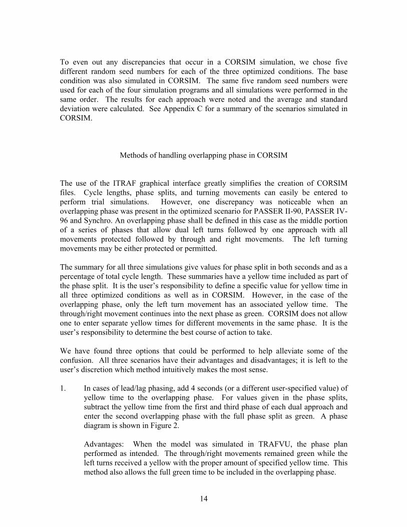
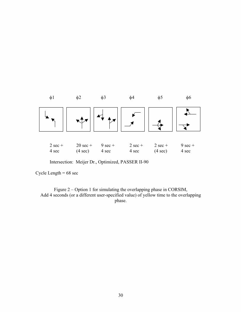
Methods of handling overlapping phase in CORSIM The use of the ITRAF graphical interface greatly simplifies the creation of CORSIM files. Cycle lengths, phase splits, and turning movements can easily be entered to perform trial simulations. However, one discrepancy was noticeable when an overlapping phase was present in the optimized scenario for PASSER II-90, PASSER IV-96 and Synchro. An overlapping phase shall be defined in this case as the middle portion of a series of phases that allow dual left turns followed by one approach with all movements protected followed by through and right movements. The left turning movements may be either protected or permitted. The summary for all three simulations give values for phase split in both seconds and as a percentage of total cycle length. These summaries have a yellow time included as part of the phase split. It is the user’s responsibility to define a specific value for yellow time in all three optimized conditions as well as in CORSIM. However, in the case of the overlapping phase, only the left turn movement has an associated yellow time. The through/right movement continues into the next phase as green. CORSIM does not allow one to enter separate yellow times for different movements in the same phase. It is the user’s responsibility to determine the best course of action to take. We have found three options that could be performed to help alleviate some of the confusion. All three scenarios have their advantages and disadvantages; it is left to the user’s discretion which method intuitively makes the most sense. 1. In cases of lead/lag phasing, add 4 seconds (or a different user-specified value) of

yellow time to the overlapping phase. For values given in the phase splits, subtract the yellow time from the first and third phase of each dual approach and enter the second overlapping phase with the full phase split as green. A phase diagram is shown in Figure 2.

Advantages: When the model was simulated in TRAFVU, the phase plan performed as intended. The through/right movements remained green while the left turns received a yellow with the proper amount of specified yellow time. This method also allows the full green time to be included in the overlapping phase.

15

Disadvantages: While the TRAFVU model is an accurate representation of the CORSIM file, it may not be an exact representation. TRAFVU was developed after CORSIM, not as part of the actual model. As a result, what appears in TRAFVU may not actually be what is modeled in CORSIM. In addition, the cycle length is increased by the yellow time multiplied by the number of overlapping phases. It is possible that this increase in cycle length changes the MOEs in the simulation.

2. CORSIM does not allow a user to input a value of zero for any phase or yellow

time. Therefore, to limit the disruption to the simulated condition obtained from other programs, the overlapping phase’s yellow time is reduced to one second (the minimum value) and the following phase’s yellow time is reduced by one second. A phase diagram is shown in Figure 3.

Advantages: Because of the reduction in the yellow time of the phase following the overlap, cycle length is kept constant. It also limits differences between the CORSIM runs and the optimized condition from other simulation programs. Disadvantages: While the cycle length is kept constant, the actual green time is not quite the same as that given in the optimized condition. Sometimes under high traffic volumes, even a slight difference in green time and phase split can increase delay time substantially. Thus, it may not give an accurate representation of an optimal condition.

3. Treat the overlapping phase the same as the other phases, reduce the phase split

by the yellow time and proceed accordingly. A phase diagram is shown in Figure 4.

Advantages: The major advantage of this scenario is that all phases are treated the same. In addition, there is no change in cycle length from what is obtained in each of the trial runs. Disadvantages: Some overlapping phases have a length less than the yellow time. If yellow time were to be subtracted from the phase length, the phase would be negative, an impossible task. If green time for a phase were to become negative, it would be easiest to eliminate the phase altogether and subtract the remaining time from the preceding and following phases. Hence, the progression would most likely not be the same as the plan from the optimized condition.

For this analysis, we chose the first method of yellow split and overlapping phases. There is no simple way to determine if this is actually correct, but the method was employed consistently for all CORSIM runs. It is left to the user’s discretion to decide which method is most logical. However, if cycle length continuity and representing each phase the same is most important, method 3

16

should be adopted. If cycle length continuity and an adherence to TRAFVU output with limitations on disturbing optimized scenarios is most important, method 2 should be adopted. If green time continuity and conformance with the output in TRAFVU is most important, method 1 should be adopted.

STATISTICAL ANALYSIS OF RESULTS Because of the different phase timings in each condition, it was necessary to devise a method of quantifying the results given for each simulation. First, HCS-97 base condition MOEs were compared to Synchro base condition MOEs. Second, the optimized timings obtained through Synchro were modeled in CORSIM using the three methods of yellow timing stated previously. Five runs for each method were performed using the same random seed numbers for each trial. These results were compared to each other. The process was repeated for both PASSER II-90 and PASSER IV-96 timings. Third, the results for all three optimized timings were compared to each other, Synchro vs. PASSER II-90, Synchro vs. PASSER IV-96, and PASSER II-90 vs. PASSER IV-96 as well as to the CORSIM-run for the base condition. Approach, intersection and network control delays were determined for each condition. These conditions were compared to the base condition delays (HCS-97) as well as to each other. A paired t-test and a regression analysis were used to compare base conditions of HCS-97 and Synchro. Similarly, a paired t-test was used to make the comparison between CORSIM optimized runs of Synchro, PASSER II-90, and PASSER IV-96. For the regression analysis comparing base condition data, movement delays for each intersection were compared between HCS-97 and Synchro Ver.4.0. Three conditions were compared: HCS-97 vs. Synchro (Actuated-Coordinated) and HCS-97 vs. Synchro (Actuated-Uncoordinated) and HCS-97 vs. Synchro (Pretimed). Ideally, if both simulations were to compute identical results, a 45-degree line starting at (0,0) could be fit to the data. In this case, the coefficient of determination (R2) is a measure of linearity. The closer R2 gets to 1, the better the line fits the data. A paired t-test was also used to compare movement delay between HCS-97 and Synchro. The paired t-test allows one to compare each individual movement in one simulation to the same movement in a different simulation. The difference in individual movements was found then summed together and averaged. The equation for the paired t-test can then be used as follows: t = (∆ - 0) / (S / (N).5) Where:

17

∆ = average difference between movement delays S = standard deviation of the differences N = number of traffic movement in the network The t value can then be compared to a table value and a probability can be ascertained on the compatibility of the two simulations. In addition to comparing simulations to each other, it is also necessary to make comparisons within simulation runs. Because of the discrepancies that exist in CORSIM, determining whether the method of yellow time splits makes a significant difference in approach delay is helpful. If there were no significant difference, any method could be used and results could be inferred to be the same no matter which course of action were taken. If the difference were noticeable, how noticeable would it be and should one method be used over another? The equation used in CORSIM comparisons is as follows: t = (XCOR1 – XCOR2) / [(((n1 – 1)S1

2 + (n2 – 1)S22) / (n1 + n2 –2)) * (n1

-1 + n2-1)].5

Where: XCOR1 = average approach delay value for method 1 XCOR2 = average approach delay value for method 2 n1 = number of trial runs for method 1 n2 = number of trial runs for method 2 S1 = standard deviation for method 1 S2 = standard deviation for method 2 COMPARISONS OF THE RESULTS Base Condition In the base condition, three scenarios were used:

1. The existing signal settings and traffic volume assuming actuated-coordinated controller

2. The existing signal settings and traffic volume assuming actuated-uncoordinated controller

3. The existing signal settings and traffic volume assuming Pretimed traffic controller

Each scenario was modeled in HCS-97 and Synchro 4.0. PASSER II-90 and PASSER IV-96 were not included in the base condition comparison because they are not able to simulate the existing conditions due to different cycle lengths.

18

Synchro calculations with right turn on red (RTOR) enabled will not be compatible with HCM results. This is because the HCM does not utilize RTOR in its calculations. Therefore, to eliminate the discrepancies in results due to this difference, we modeled the eight selected intersections with “No Right Turn on Red”. The RTOR calculations in Synchro are based on an internally developed model based on the HCM gap acceptance formula for right turns. Lost time in Synchro and HCS is defined in the same way when there is not a protected left turn movement proceeding to the next time interval as permitted left turn. When there exists such a phasing plan, Synchro assumes 0.5 sec all red time between protected and permitted phase. This causes some discrepancies between lost time calculated in Synchro and HCS. This directly affects the delay calculations. To avoid entering data differently for each model, data entered in Synchro were exported to HCS. HCS, unlike Synchro, is not capable of modeling a situation where there are two simultaneous phases with one of them terminating ahead of the other. The phase plans used in this study were all terminated simultaneously. Synchro, unlike HCS, does not require Arrival Type as input item. Instead of using Arrival Type to determine progression adjustment factor, Synchro calculates the progression factor by looking at the arrivals from the upstream intersections and routing them through the subject intersection. If we take the Synchro PF and the corresponding g/C and determine the Arrival Type based on the definition of Chapter 9 of HCM, the result will be different than the Arrival Type that appears in HCS after exporting the data from Synchro. The net effect of thes discrepancies is that different progression factors are used in Synchro and HCS. PF directly affects delay calculations. Tables 2-A through 4-B presented in Appendix A show comparison between the three base condition scenarios. For Pretimed scenario, overall, 1.6% of HCS control delay values differ by 10% or more from Synchro computed values. Once again, the paired t-test showed that the difference between the HCS control delays and Synchro computed values was statistically insignificant (p-value = 0.293). Only 3.2% of HCS computed uniform delay values differ by 10% or more from Synchro computed values. For the incremental delay, d2, 9.5% of HCS computed values differ by 10% or more from Synchro computed values. The differences in d1 and d2 computed by both software were not statistically significant (p-value=0.075 and 0.112). Figure 5 shows that the correlation between the HCS incremental delays and Synchro incremental delays is the strongest among the three considered scenarios for traffic controller. For actuated coordinated and actuated uncoordinated, Synchro and HCS are modeling different traffic conditions, even though data is imported to HCS. However, in this study we compared the output for the sake of completeness. The following two paragraphs should be read with this in mind.

19

For actuated coordinated controller, overall, 33% of HCS control delay values differ by 10% or more from Synchro computed values. Paired t-test showed that the difference between the HCS control delays and Synchro computed values was statistically significant (p-value = 0.02). These results were not expected because Synchro software bases delay calculation off of criteria set forth in the HCM-97. The difference in d1 and d2 computed by Synchro and HCM were further examined and their values were not statistically different. However, d1PF was significantly different. The comparison results show that 8% of HCS computed uniform delay (d1) values differ by 10% or more from Synchro computed values. On the other hand, 33% of (d1×PF) values computed by HCS differ by 10% or more from Synchro comparable values. For the incremental delay, d2, 46% of HCS computed values differ by 10% or more from Synchro computed values. Figure 6 shows the regression line between HCS incremental delays and Synchro incremental delays. As shown, there is a good correlation between the two delay values. However, the values are not identical. For uncoordinated intersections, the progression adjustment factor is 1.0 because the arrival is random. In this case, overall, 17.5% of HCS control delay values differ by 10% or more from Synchro computed values. However, the paired t-test showed that the difference between the HCS control delays and Synchro computed values was statistically insignificant (p-value = 0.366). The comparison results show that 9.5% of HCS computed uniform delay values differ by 10% or more from Synchro computed values. For the incremental delay, d2, 60% of HCS computed values differ by 10% or more from Synchro computed values. However, the differences in d1 and d2 computed by Synchro and HCM were not statistically significant (p-value=0.478 and 0.412). Figure 7 shows that the correlation between the HCS incremental delays and Synchro incremental delays is relatively weaker than the comparable relation for actuated-coordinated controller. Optimized Condition Four different measures of effectiveness were analyzed for the optimized condition. They include the movement delay, the approach delay, the intersection delay and the network delay. The movement delay is based on the individual movements of an intersection, such as westbound left turns or northbound through traffic. Approach delay is the weighted average based on traffic volumes of the movement. Intersection delay is the weighted average based on traffic volumes of all approaches. Network delay is the sum of the intersection delays for each of the traffic simulation models. Four scenarios were presented for comparison: HCS-97 (base condition) as a datum, Synchro optimized condition, PASSER II-90 optimized condition and PASSER IV-96 optimized condition. The comparison shows that movement delays for each of the four scenarios vary considerably. There appears to be no correlation among any of the four models. For example, delays for the westbound left turn movement at the intersection including Marketview Dr. vary from 17.7 seconds in HCS-97 to 52.2 seconds per vehicle

20

in PASSER II. This ranges from a LOS B to LOS D. There does appear, however, to be a slightly better correlation for lightly traveled intersections than those that are more heavily traveled. The approach delays for the four scenarios vary as well, though not as considerably as for the movement delays. Again, there appears to be more agreement among intersections that have less traffic, such as Baytowne Drive and Town Center Drive. Table 5 shows the results of paired t-test to determine whether the approach delays in the optimized condition any better than those in the base condition. The results showed that the optimized condition in PASSER II and PASSER IV are not significantly different from the base condition (p-value =0.344, 0.169 respectively). Approach delays for the optimized condition in Synchro were significantly lower than the delays in the base condition (p-value = 0.000).

Table 5. t-Test for Approach Delay: Paired Two Sample for Means (Is the optimized condition any better than the base condition?)

Approach Delay Model

Mean Variance t Statistic p-value

HCS-97 (base) 24.4 173.14 -

Synchro 15.4 27.28 4.13 0.000 PASSER II 25.6 148.19 -0.41 0.344 PASSER IV 22.3 40.01 0.97 0.169

t Critical one-tail = 1.699, n = 30

Table 6. t-Test for Intersection Delay: Paired Two Sample for Means (Is the optimized condition any better than the base condition?)

Intersection Delay Model

Mean Variance t Statistic p-value

HCS-97 (base) 23.8 153.67 -

Synchro 15.4 15.22 2.28 0.028 PASSER II 20.4 38.43 0.97 0.182 PASSER IV 20.4 23.66 0.99 0.178

t Critical one-tail = 1.895, n = 8

The intersection delays for Synchro were significantly less than the intersection delays obtained for the base condition. Optimized conditions suggested by PASSER II and PASSER IV produced intersection delays that were not, however, significantly different

21

from intersection delays for the base conditions (p-value = 0.178 and 0.182 respectively) as shown in Table 6. The network delay for the four scenarios varied, though the delay for PASSER II-90 and PASSER IV-96 are nearly identical (163.5 and 163.0 sec/veh respectively). The delay for Synchro is appreciably less (123.2 sec/veh). The base condition gives the highest network delay (190.6 sec/veh), which is expected, since the other three software attempt to improve on a given condition provided the base condition is not already improved. Optimized Conditions simulated in CORSIM In this study, CORSIM was used as a control to obtain prescribed MOEs for the base conditions and each of the three optimized scenarios. Through the use of CORSIM, we were able to make a second comparison using a controlled simulation and detect similarities and differences between the various traffic models. One of the major differences between CORSIM and the other traffic simulation programs in this study is that CORSIM does not calculate individual movement delays. The smallest unit of comparison is approach delays. Hence, only approach delay, intersection delay, and network delay comparison can be made using CORSIM results. Again, four scenarios were presented for comparison: base condition simulated in CORSIM and the three optimized conditions (Synchro, PASSER II and PASSER IV) simulated in CORSIM. The approach delay for the four scenarios are varied, but less than the approach delay for the optimized condition previously stated. For example, the intersection containing Lowe’s Dr with southbound traffic had delays ranging from 12.7 seconds to 14.6 seconds per vehicle as shown in Figure 8. The four values fall within a very small range. However, there appears to be a greater difference in delay times between models when traffic through the intersection increases as opposed to lightly traveled intersections. Overall, the differences in approach delays resulted from simulating the optimized conditions suggested by Synchro and PASSER IV in CORSIM were not significantly different from approach delays for the base conditions when simulated in CORSIM (p-value = 0.513 and 0.386) as shown in Table 7. However, the differences in approach delays resulted from simulating the optimized conditions suggested by PASSER II were not significantly higher than the delay for base conditions with 95% confidence, but were significantly higher with 90% confidence (p-value = 0.076).

22

0

5

10

15

20

25

30

35

EB WB NB SB Intersection

Con

trol D

elay

, sec

/veh

CORSIM

Synchro (1)

PASSER IV-96 (1)

PASSER II-90 (1)

Meijer Dr.

0

5

10

15

20

25

30

35

40

EB WB NB SB Intersection

Con

trol D

elay

, sec

/veh

CORSIM

Synchro (1)

PASSER IV-96 (1)

PASSER II-90 (1)

Town Center Dr.

0

5

10

15

20

25

30

35

40

EB WB NB SB Intersection

Con

trol D

elay

, sec

/veh

CORSIM

Synchro (1)

PASSER IV-96 (1)

PASSER II-90 (1)

Baytowne Dr.

0

5

10

15

20

25

30

35

40

EB WB NB SB Intersection

Con

trol D

elay

, sec

/veh

CORSIM

Synchro (1)

PASSER IV-96 (1)

PASSER II-90 (1)

Lowe's Dr.

Figure 8. Comparison of delays computed by CORSIM, Synchro and PASSER for 8 intersections for optimized conditions

23

0

10

20

30

40

50

60

Con

trol D

elay

, sec

/veh

CORSIM

Synchro (1)

PASSER IV-96 (1)

PASSER II-90 (1)

Marketview Dr.

0

5

10

15

20

25

30

Con

trol D

elay

, sec

/veh

CORSIM

Synchro (1)

PASSER IV-96 (1)

PASSER II-90 (1)

I-74 WB ramps

0

5

10

15

20

25

30

35

Con

trol D

elay

, sec

/veh

CORSIM

Synchro (1)

PASSER IV-96 (1)

PASSER II-90 (1)

I-74 EB ramps

0

10

20

30

40

50

60

70

Con

trol D

elay

, sec

/veh

CORSIM

Synchro (1)

PASSER IV-96 (1)

PASSER II-90 (1)

Bloomington Rd.

Figure 8 (cont). Comparison of delays computed by CORSIM, Synchro and PASSER for 8 intersections for optimized conditions

24

Table 7. t-Test for Approach Delay: Paired Two Sample for Means (Is the optimized condition obtained by a specific software any different than the

optimized condition simulated in CORSIM?)

Approach Delay Model Mean Variance

t Statistic p-value

CORSIM (base) 18.5 88.71 -

Synchro 17.9 50.58 0.663 0.513 PASSER II 23.1 130.62 -1.839 0.076 PASSER IV 19.9 120.28 -0.880 0.386

t Critical two-tail = 2.045, n = 30

The intersection delay for the four scenarios is noticeably close for the majority of the intersections. The optimized conditions of Synchro, PASSER II and PASSER IV when simulated in CORSIM yielded intersection delays that were not significantly different from intersection delays for the base conditions when simulated in CORSIM (p-value = 0.678, 0.879 and 0.704 respectively) as shown in Table 8.

Table 8. t-Test for Intersection Delay: Paired Two Sample for Means (Is the optimized condition obtained by a specific software any different than the

optimized condition simulated in CORSIM?)

Intersection Delay Model Mean Variance

t Statistic p-value

CORSIM (base) 19.1 59.33 -

Synchro 18.4 20.22 0.433 0.678 PASSER II 19.4 37.00 -0.158 0.879 PASSER IV 19.7 55.59 -0.395 0.704

t Critical two-tail = 2.365, n = 8

As shown in Figure 9, the network delay for the four scenarios are very similar, though delay for Synchro is slightly less than the delay for the other three simulated conditions. One would expect to encounter a situation similar to the optimized results, that delay for the optimization programs would be less than that for the base condition. This was not the case. In two of the scenarios the opposite was the outcome, though by just a slight margin.

25

Figure 9. Comparison of Network delays computed by CORSIM, Synchro and PASSER

For optimized conditions

140

142

144

146

148

150

152

154

156

158

160

Con

trol D

elay

, sec

/veh

CORSIM Synchro (1) PASSER_IV-96(1) PASSER II-90(1)

26

ISSUES IN COMPARING HCM AND SYNCHRO To avoid entering data differently for each model, data entered in Synchro should be imported to HCS. HCS is not capable of modeling a situation where two simultaneous phases exist with one of them terminates ahead of the other, but Synchro is. For such situations, these two software can not be compared. For phases that terminate simultaneously, the user must take the following precautions before comparing Synchro and HCM outputs. Even with these precautions, the user will be modeling different traffic conditions, except for pretimed uncoordinated traffic condition. Pretimed uncoordinated Controllers 1. Disable RTOR in Synchro for the calculations to be compatible with HCM. The

HCM does not utilize right turn on red calculations. 2. Eliminate all red time in Synchro when a protected left turn movement proceeds to

the next time interval as permitted left turn to make the total lost time in Synchro and the HCS the same

Pretimed coordinated Controller 1. Step 1 and 2 described under pretimed uncoordinated controllers. 2. PF values used in Synchro and HCM are different. There is no easy solution to fix

this discrepancy. Actuated uncoordinated 1. The signal split imported to HCS are different than those used by Synchro Actuated coordinated 1. Same as number 1 in actuated uncoordinated. 2. Same as number 2 in pretimed coordinated.

27

CONCLUSIONS AND RECOMMENDATIONS This study compared control delays computed by HCM (using HCS software), Synchro, PASSER and CORSIM to highlight the similarities and differences. The software were evaluated under two conditions: base condition and optimized condition. In the base condition, the existing signal settings and traffic volumes were modeled in HCS-97 and Synchro 4.0 under three scenarios: actuated-coordinated, actuated-uncoordinated and pretimed traffic controller. PASSER II-90 and PASSER IV-96 were not included in the base condition comparison because they could not simulate the existing signal timings with different cycle lengths. Base Condition User should be aware that HCS shouldn’t be directly compared to Synchro unless certain precautions are taken in running Synchro. These precautions are outlined in the section entitled “ISSUES IN COMPARING HCM AND SYNCHRO”. For both pretimed and actuated, if simultaneous phases exist with one of them terminates ahead of the others, the results of HCS and Synchro are not comparable. For both pretimed and actuated signals where the phases terminate simultaneously, whether the data is imported from Synchro or manually entered in HCS, the condition analyzed won’t be comparable unless the precautions described previously are taken. We took these precautions to make the conditions analyzed in Synchro comparable to those analyzed in HCS. Once these precautions were taken, control delays from Synchro and HCM were not significantly different for pretimed uncoordinated signals. For actuated-uncoordinated and for actuated-coordinated, the software are modeling different conditions, though they may appear similar, the comparison are not meaningful. Optimized Condition For actuated coordinated signal controllers, the software optimized signal settings and calculated the delays. The delays for optimized conditions for PASSER II and PASSER IV were not significantly different than the delays before optimization. However, for Synchro, the delays for optimized conditions were significantly lower than the delays before optimization. To verify if the optimized conditions will produce lower delay if implemented in the field, the new signal settings were used to simulate the optimized conditions in CORSIM. If optimized signal settings suggested by PASSER II, PASSER IV or Synchro implemented, the delays for optimized condition would not be significantly lower than the delays before optimization. Even though Synchro gives the impression that delays were significantly different than the delays before optimization, the lower delays calculated by Synchro for optimized condition were not verified.

28

All five programs possess distinct advantages and disadvantages, which shall be outlined below. HCS Advantages: The Highway Capacity Software is used by many agencies in determining capacity and LOS. The newest version, HCS-97 and HCS 2000, are Windows based and much easier to use than the older HCS-94. HCS-97 also calculates delay values as soon as input parameters are changed, as opposed to the old HCS software that had to be run every time inputs were altered. Disadvantages: HCS does the calculation for existing conditions. It doesn’t optimize signal setting. Signal timings must be altered manually and be compared to previous entries. For this study, optimization for HCS was not used because it varies from user to user. Synchro Advantages: The advantage of Synchro is its interface. One creates a network by drawing links on a given pallet, a good visualization tool none of the other programs possess. Synchro can model existing conditions and determines optimal signal settings Disadvantages: Synchro is a fairly new program and is not used as widespread as some of the other programs in this study. In addition, Synchro tended to return delay values that were lower than the other programs, sometimes substantially lower. Further analysis might be necessary to validate the results. There is a new version of Synchro (5.0) that is based on the 2000 Highway Capacity Manual. PASSER II-90 Advantages: PASSER II-90 is still used by some agencies. It is fairly easy to use, once one gets acclimated to the DOS shell. PASSER II-90 also calculates the optimal offset between signal timings on a network. Disadvantages: PASSER II-90 is DOS-based and not especially user friendly. It does not model exclusive right turn lanes and cannot account for right turns on red. The DOS shell is difficult to navigate and it is cumbersome to load existing networks. The separate input and output files are confusing. Only one arterial can be analyzed at a time. PASSER II-90 cannot model existing conditions and can only return optimal conditions with identical cycle lengths for a multiple intersection network.

29

PASSER IV-96 Advantages: PASSER IV-96 is also a DOS based program that is easy to understand. PASSER IV-96 is able to optimize networks in a similar fashion to that of PASSER II-90. Unlike PASSER II-90, PASSER IV-96 can model multiple arterials and up to 40 intersections. Disadvantages: PASSER IV-96 is more user friendly than PASSER II-90, but the DOS shell can be a bit confusing. The program can not easily model existing conditions and may return an error message if specified cycle lengths are too long even though they may be reasonable. PASSER IV-96 can not model exclusive right turn lanes and will not give a delay calculation for right turn movements. CORSIM Advantages: With the ITRAF graphical input method and the TRAFVU graphical output, CORSIM is easier to use and understand now. It is regarded as a key tool in traffic simulation. CORSIM takes driver characteristics, such as reaction time, acceleration/deceleration, and driver aggressiveness into account in simulation runs, the other software does not. In this case, CORSIM was considered a standard of comparison between the other analyzed software. Disadvantages: Coding CORSIM is not straightforward and the user has to have a fair knowledge of traffic simulation issues. MOE calculations can be long, complicated, and sometimes difficult to understand. Though they are not perfect, the availability of traffic simulation models greatly expands opportunities for development of new and innovative transportation systems management (TSM) concepts. These models can provide the transportation planner with information to identify weaknesses in concepts and design for traffic flow analysis. They can facilitate the identification of an optimal solution among many choices.

30

φ1 φ2 φ3 φ4 φ5 φ6

2 sec + 20 sec + 9 sec + 2 sec + 2 sec + 9 sec + 4 sec (4 sec) 4 sec 4 sec (4 sec) 4 sec Intersection: Meijer Dr., Optimized, PASSER II-90 Cycle Length = 68 sec

Figure 2 – Option 1 for simulating the overlapping phase in CORSIM, Add 4 seconds (or a different user-specified value) of yellow time to the overlapping

phase.

31

φ1 φ2 φ3 φ4 φ5 φ6

2 sec + 20 sec + 9 sec + 2 sec + 2 sec + 9 sec + 4 sec (1 sec) 3 sec 4 sec (1 sec) 3 sec Intersection: Meijer Dr., Optimized, PASSER II-90 Cycle Length = 60 sec Figure 3 – Option 2 for simulating the overlapping phase in CORSIM assume the yellow

time for the overlapping phase to be one second (the minimum value) and deduct this second from the following phase’s yellow time.

32

+- φ1 φ2 φ3 φ4 φ5

2 sec + 16 sec + 9 sec + 2 sec + 11 sec + 4 sec (4 sec) 4 sec 4 sec 4 sec Intersection: Meijer Dr., Optimized, PASSER II-90 Cycle Length = 60 sec Figure 4 – Option 3 for simulating the overlapping phase in CORSIM reduce the phase split by the yellow time and proceed accordingly

33

APPENDIX A: BASE CONDITION

34

Table 2.A. HCS-97 vs Synchro 4.0 (Actuated-Coordinated)

35

Table 2.B. HCS-97 vs Synchro 4.0 (Actuated-Coordinated)

36

Table 3.A. HCS-97 vs Synchro 4.0 (Actuated-Uncoordinated)

37

Table 3.B. HCS-97 vs Synchro 4.0 (Actuated-Uncoordinated)

38

Table 4.A. HCS-97 vs Synchro 4.0 (Pretimed)

39

Table 4.B. HCS-97 vs Synchro 4.0 (Pretimed)

40

Figure 5. Comparison of incremental delay values (d2) computed by both HCS-97 and Synchro 4.0 for

8 pretimed intersections

41

Figure 6. Comparison of incremental delay values (d2) computed by both HCS-97 and Synchro 4.0 for

8 actuated-coordinated intersections

42

Figure 7. Comparison of incremental delay values (d2) computed by both HCS-97 and Synchro 4.0 for

8 actuated-uncoordinated intersections

43

APPENDIX B: SUMMARIZED DATA, OPTIMIZED CONDITION

44

45

APPENDIX C: SUMMARIZED DATA, CORSIM OPTIMIZED CONDITION

46

47

48

REFERENCES 1. Highway Capacity Manual, 3rd Edition, 1998. 2. Thor, Carl and Chen, Hobih, “Understanding the Cumulative Statistics from TRAF-NETSIM”, PC-

TRANSmission, University of Kansas Transportation Center, 1989 Oct: 1-2. 3. Traffic Analysis Software. TRB Circular Number E-CO14, National Research Council,

Washington, D.C, September 2000.