Comparison of Biclustering Methods: A

Systematic Comparison and Evaluation of

Biclustering Methods for Gene Expression Data

Amela Prelic,a Stefan Bleuler a, Philip Zimmermann b,Anja Wille c,d, Peter Buhlmann d, Wilhelm Gruissem b,

Lars Hennig b, Lothar Thiele a, and Eckart Zitzler a

Reverse Engineering Group:aComputer Engineering and Networks Laboratory

bInstitute for Plant Sciences and Functional Genomics Center ZurichcColab

dSeminar for Statistics, ETH Zurich, Switzerland

TIK-Report No. 227Computer Engineering and Networks Laboratory

ETH ZurichGloriastrasse 35, ETH-Zentrum, 8092 Zurich, Switzerland

Revised VersionFebruary 2006

(First Version: July 2005)

Abstract

Motivation: In recent years, there have been various efforts to over-come the limitations of standard clustering approaches for the analysisof gene expression data by grouping genes and samples simultaneously.The underlying concept, which is often referred to as biclustering, allowsto identify sets of genes sharing compatible expression patterns acrosssubsets of samples, and its usefulness has been demonstrated for differentorganisms and data sets. Several biclustering methods have been proposedin the literature; however, it is not clear how the different techniques com-pare to each other with respect to the biological relevance of the clustersas well as to other characteristics such as robustness and sensitivity tonoise. Accordingly, no guidelines concerning the choice of the biclusteringmethod are currently available.

1

Results: First, this paper provides a methodology for comparing andvalidating biclustering methods that includes a simple binary referencemodel. Although this model captures the essential features of most bi-clustering approaches, it is still simple enough to exactly determine alloptimal groupings; to this end, we propose a fast divide-and-conquer al-gorithm (Bimax). Second, we evaluate the performance of five salientbiclustering algorithms together with the reference model and a hierar-chical clustering method on various synthetic and real data sets for Sac-

charomyces cerevisiae and Arabidopsis thaliana. The comparison revealsthat (i) biclustering in general has advantages over a conventional hier-archical clustering approach, that (ii) there are considerable performancedifferences between the tested methods, and that (iii) already the simplereference model delivers relevant patterns within all considered settings.

Availability: The data sets used, the outcomes of the biclusteringalgorithms under consideration, and the Bimax implementation for thereference model are available at http://www.tik.ee.ethz.ch/sop/bimax

Contact: bleuler@tik.ee.ethz.ch, zitzler@tik.ee.ethz.ch

1 Introduction

In recent years, several biclustering methods have been suggested to identifylocal patterns in gene expression data. In contrast to classical clustering tech-niques such as hierarchical clustering (Sokal and Michener, 1958), and k-meansclustering (Hartigan and Wong, 1979), biclustering does not require genes inthe same cluster to behave similarly over all experimental conditions. Instead,a bicluster is defined as a subset of genes that exhibit compatible expressionpatterns over a subset of conditions. This modified clustering concept can beuseful to uncover processes that are active only over some but not all samplesas has been demonstrated in several studies (Cheng and Church, 2000; Ihmelset al., 2002; Ben-Dor et al., 2002; Tanay et al., 2002; Murali and Kasif, 2003),see (Madeira and Oliveira, 2004) for a survey.

Comparing clustering methods in general is difficult as the formalization interms of an optimization problem strongly depends on the scenario under con-sideration and accordingly varies for different approaches. In the end, biologicalmerit is the main criterion for validation, though it can be intricate to quantifythis objective. In the literature, there are several comparative studies on tradi-tional clustering techniques (Yeung et al., 2001; Azuaje, 2002; Datta and Datta,2003); however, for biclustering no such extensive empirical comparisons existas pointed out by (Madeira and Oliveira, 2004). Although first steps in thisdirections have been made (Tanay et al., 2002; Yang et al., 2003; Ihmels et al.,2004), the corresponding studies focus on validating a new algorithm with re-gard to one or two existing biclustering methods and usually consider a specificobjective function.

The main goal of this paper is to provide a systematic comparison andevaluation of prominent biclustering methods in the light of gene classification.In particular, we address the following questions:

2

• What comparison and validation methodology is adequate for the biclus-tering context?

• How meaningful are the biclusters selected by existing methods?

• How do different methods compare to each other: do some techniques haveadvantages over others or are there common properties that all approachesshare?

In order to answer these questions, we have selected a number of salientbiclustering methods, implemented them, and tested them on both syntheticand real gene expression data sets. An in silico scenario has been chosen to (i)investigate the capability of the algorithms to recover implanted transcriptionmodules (Ihmels et al., 2002), i.e., sets of co-regulated genes together with theirregulating conditions, and to (ii) study the influence of regulatory complexityand noise on the performance of the algorithms. To assess the biological rel-evance of biclusters on gene expression data for Saccharomyces cerevisiae andArabidopsis thaliana, multiple quantitative measures are introduced that relatethe biclustering outcomes to annotations by (The Gene Ontology Consortium,2000), metabolic pathway maps, and protein-interaction data.

Moreover, we propose a simple biclustering model, which retains commonfeatures of most biclustering methods, in combination with a fast and exactalgorithm (Bimax)—in contrast, existing biclustering algorithms usually do notguarantee to find global optima. Although restricted from a biological point ofview, this model allows to study the validity of the biclustering idea independentof the interfering effects due to approximate algorithms. As such, Bimax hasbeen considered as a reference method in our study. As will be shown in the re-mainder of this paper, even such a simple approach delivers biologically relevantresults and compares well with more sophisticated biclustering methods.

2 Related Work

There exist several studies that address the issue of comparing and validatingone-dimensional clustering methods (Kerr and Churchill, 2001; Yeung et al.,2001; Azuaje, 2002; Datta and Datta, 2003; Gat-Viks et al., 2003; Handl et al.,2005). All of them make use of different quantitative measures or validity in-dices, which can be divided into three categories (Halkidi et al., 2001): internal,external, and relative indices. Internal indices solely rely on the input data—examples are the two measures of homogeneity and separation (Gat-Viks et al.,2003). In contrast, external criteria are based on additional data in order tovalidate the obtained results. In the context of gene expression data, thesewould correspond to prior biological knowledge of the systems being studied;alternatively, a validation can be done by referring to other types of genomicdata representing similar aspects of the regulation mechanisms being investi-gated. The third category of relative indices measures the influence of the inputparameter settings on the clustering outcome. As discussed in (Handl et al.,

3

2005), external indices are preferable in order to assess the performance of analgorithm on a given data set, while internal indices can be used to investigatewhy a particular method does not perform well.

In the context of biclustering, mainly external validation has been used.Biological analyses and interpretations by human experts are most commonfor the evaluation of a single, newly proposed biclustering algorithm (Chengand Church, 2000; Getz et al., 2000; Ben-Dor et al., 2002; Murali and Kasif,2003; Bergmann et al., 2003; Getz et al., 2003; Ihmels et al., 2004); they areusually descriptive and qualitative only, and therefore not suited for comparingmultiple methods. In terms of quantitative measures, many papers rely onknown classifications and categorizations given by tumor types (Tanay et al.,2002; Kluger et al., 2003; Murali and Kasif, 2003), GO annotations (Tanayet al., 2002; Tanay et al., 2004), metabolic pathways (Ihmels et al., 2002), orpromoter motifs (Ihmels et al., 2004), which are closely related to the specificdata sets under consideration. Some authors also investigate in silico datasets with implanted biclusters where the optimal outcome is known beforehand(Ihmels et al., 2002; Ben-Dor et al., 2002; Bergmann et al., 2003; Yang et al.,2002).

Most biclustering papers are concerned with the introduction and valida-tion of a new approach, while only a few contain quantitative comparisons toexisting methods. (Cheng and Church, 2000), and (Kluger et al., 2003), val-idate the biclustering results in comparison to hierarchical clustering and sin-gular value decomposition respectively. (Tanay et al., 2002), and (Yang et al.,2002; Yang et al., 2003), provide a comparison to the algorithm by (Cheng andChurch, 2000), regarding synthetic data respectively the problem formulationintroduced in (Cheng and Church, 2000). In (Ihmels et al., 2004), two biclus-tering techniques (Cheng and Church, 2000; Getz et al., 2000) as well as fiveclassical clustering methods are tested with respect to the problem formulationused by the iterative signature algorithm proposed in (Ihmels et al., 2002). Inmost of the studies, the comparison has been carried out with regard to thegene dimension.

3 Biclustering Methods

3.1 Selected Algorithms

Five prominent biclustering methods have been chosen for this comparativestudy according to three criteria: (i) to what extent the methods have beenused or referenced in the community, (ii) whether their algorithmic strategies aresimilar and therefore better comparable, and (iii) whether an implementationwas available or could be easily reconstructed based on the original publications.The selected algorithms are briefly described in the following; they are all basedon greedy search strategies.

4

Cheng and Church’s Algorithm (CC) (Cheng and Church, 2000) definea bicluster to be a submatrix for which the mean squared residue score is belowa user-defined threshold δ, where 0 represents the minimum possible value.In order to identify the largest δ-bicluster in the data, they propose a two-phase strategy: first, rows and columns are removed from the orginal expressionmatrix until the above constraint is fulfilled; later, previously deleted rows andcolumns are added to the resulting submatrix as along as the bicluster scoredoes not exceed δ. This procedure is iterated several times where previouslyfound biclusters are masked with random values. Recently, (Yang et al., 2003)proposed an improved version of this algorithm which avoids the problem ofrandom interference caused by masked biclusters.

Samba (Tanay et al., 2002) presented a graph-theoretic approach to biclus-tering in combination with a statistical data model. In this framework, theexpression matrix is modelled as a bipartite graph, a bicluster is defined as asubgraph, and a likelihood score is used in order to assess the significance ofobserved subgraphs. A corresponding heuristic algorithm called Samba aimsat finding highly significant and distinct biclusters. In a recent study (Tanayet al., 2004), this approach has been extended to integrate multiple types ofexperimental data.

Order Preserving Submatrix Algorithm (OPSM) In (Ben-Dor et al.,2002), a bicluster is defined as a submatrix that preserves the order of theselected columns for all of the selected rows. In other words, the expressionvalues of the genes within a bicluster induce an identical linear ordering acrossthe selected samples. Based on a stochastical model, the authors developed adeterministic algorithm to find large and statistically significant biclusters. Thisconcept has been taken up in a recent study by (Liu and Wang, 2003).

Iterative Signature Algorithm (ISA) The authors of (Ihmels et al., 2002;Ihmels et al., 2004) consider a bicluster to be a transcription module, i.e., a setof co-regulated genes together with the associated set of regulating conditions.Starting with an initial set of genes, all samples are scored with respect to thisgene set and those samples are chosen for which the score exceeds a predefinedthreshold. In the same way, all genes are scored regarding the selected samplesand a new set of genes is selected based on another user-defined threshold.The entire procedure is repeated until the set of genes and the set of samplesconverge, i.e., do not change anymore. Multiple biclusters can be identified byrunning the iterative signature algorithm on several initial gene sets.

xMotif In the framework proposed by (Murali and Kasif, 2003), biclustersare sought for which the included genes are nearly constantly expressed—acrossthe selection of samples. In a first step, the input matrix is preprocessed byassigning each gene a set of statistically significant states. These states definethe set of valid biclusters: a bicluster is a submatrix where each gene is exactly

5

in the same state for all selected samples. To identify the largest valid biclusters,an iterative search method is proposed that is run on different random seeds,similarly to ISA.

3.2 Reference Method (Bimax)

The above methods use different models which are all too complex to be solvedexactly; most of the corresponding optimization problems have shown to beNP-hard. Therefore, advantages of one method over another can be due to amore appropriate optimization criterion or a better algorithm.

To decouple these two aspects, we propose a reference method, namely Bi-max, that uses a simple data model reflecting the fundamental idea of bicluster-ing, while allowing to determine all optimal biclusters in reasonable time. Thismethod has the benefit of providing a basis to investigate

1. The usefulness of the biclustering concept in general, independently ofinterfering effects caused by approximate algorithms; and

2. The effectiveness of more complex scoring schemes and biclustering meth-ods in comparison to a plain approach.

Note that the underlying binary data model, which is described below, is onlyused by Bimax and does not represent the platform on the basis of which the dif-ferent algorithms are compared. All methods under consideration are employedusing their specific data models.

3.2.1 Model

The model assumes two possible expression levels per gene: no change andchange with respect to a control experiment.1 Accordingly, a set of m microarrayexperiments for n genes can be represented by a binary matrix En×m, wherea cell eij is 1 whenever gene i responds in the condition j and otherwise itis 0. A bicluster (G,C) corresponds to a subset of genes G ⊆ 1, .., n thatjointly respond across a subset of samples C ⊆ 1, ..,m. In other words, thepair (G,C) defines a submatrix of E for which all elements equal 1. Notethat, by definition, every cell eij having value 1 represents a bicluster by itself.However, such a pattern is not interesting per se; instead, we would like to findall biclusters that are inclusion-maximal, i.e., that are not entirely contained inany other bicluster.

Definition 1 The pair (G,C) ∈ 21,..,n×21,..,m is called an inclusion-maximalbicluster if and only if (1) ∀ i ∈ G, j ∈ C : eij = 1 and (2) 6 ∃(G′, C ′) ∈21,..,n × 21,..,m with (i) ∀ i′ ∈ G′, j′ ∈ C ′ : ei′j′ = 1 and (ii) G ⊆ G′ ∧ C ⊆C ′ ∧ (G′, C ′) 6= (G,C).

1To this end, a preprocessing step normalizes log expression values and then transformsmatrix cells into discrete values. To obtain binary values, for instance a commonly applieddiscretization procedure based on a cutoff threshold representing a twofold change can beemployed.

6

This model is similar to the one presented by (Tanay et al., 2002) whoconsider a more realistic definition of optimality where a bicluster can alsocontain 0-cells.

3.2.2 Algorithm

Since the size of the search space is exponential in n and m, an enumerativeapproach is infeasible in order to determine the set of inclusion-maximal biclus-ters. (Alexe et al., 2002) proposed an algorithm in a graph-theoretic frameworkthat can be employed in this context, if the matrix E is regarded as an adja-cency matrix of a graph. By exploiting the fact that the graph induced by E isbipartite, their incremental algorithm can be tailored to this application whichreduces the running-time complexity from Θ(n2 m2β) to Θ(nmβ log β), where βis the number of all inclusion-maximal biclusters in En×m (see supplementarymaterial). However, the memory requirements of this algorithm are of orderΩ(nmβ) which causes practical problems, especially for larger matrices.

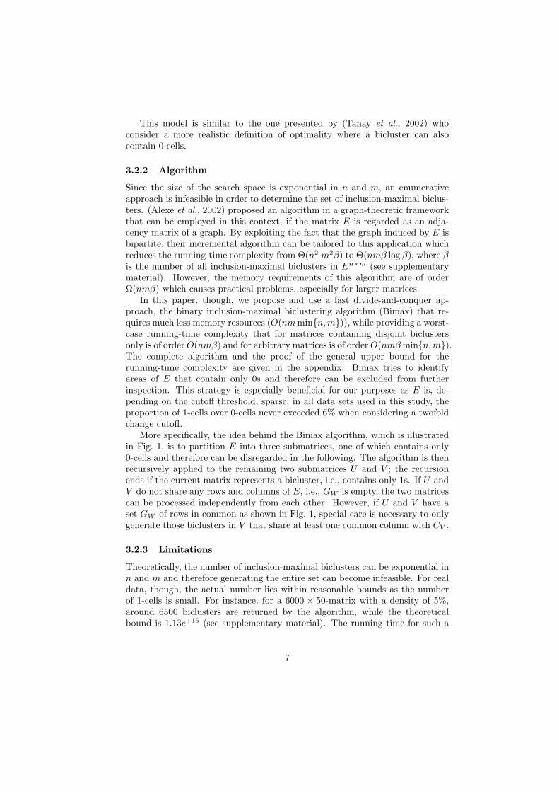
In this paper, though, we propose and use a fast divide-and-conquer ap-proach, the binary inclusion-maximal biclustering algorithm (Bimax) that re-quires much less memory resources (O(nm minn,m)), while providing a worst-case running-time complexity that for matrices containing disjoint biclustersonly is of order O(nmβ) and for arbitrary matrices is of order O(nmβ minn,m).The complete algorithm and the proof of the general upper bound for therunning-time complexity are given in the appendix. Bimax tries to identifyareas of E that contain only 0s and therefore can be excluded from furtherinspection. This strategy is especially beneficial for our purposes as E is, de-pending on the cutoff threshold, sparse; in all data sets used in this study, theproportion of 1-cells over 0-cells never exceeded 6% when considering a twofoldchange cutoff.

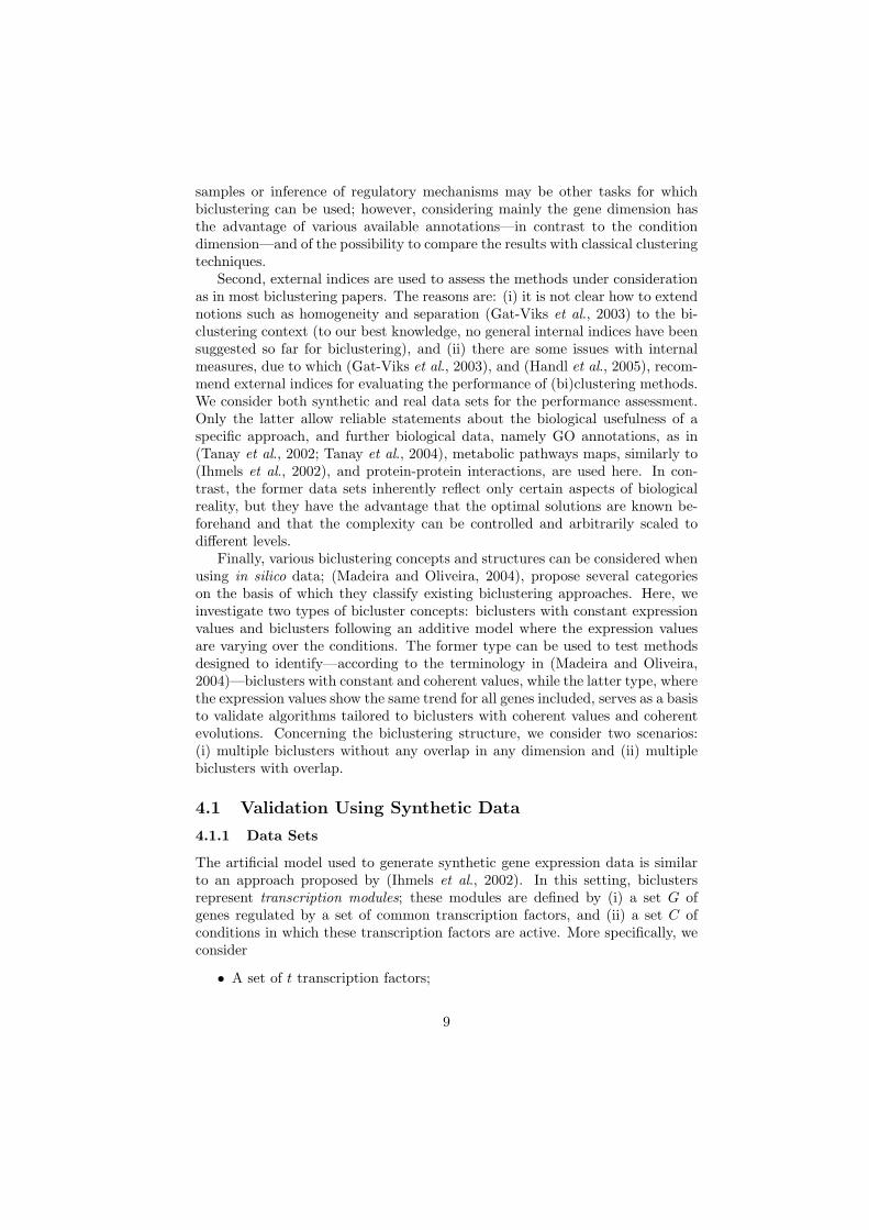
More specifically, the idea behind the Bimax algorithm, which is illustratedin Fig. 1, is to partition E into three submatrices, one of which contains only0-cells and therefore can be disregarded in the following. The algorithm is thenrecursively applied to the remaining two submatrices U and V ; the recursionends if the current matrix represents a bicluster, i.e., contains only 1s. If U andV do not share any rows and columns of E, i.e., GW is empty, the two matricescan be processed independently from each other. However, if U and V have aset GW of rows in common as shown in Fig. 1, special care is necessary to onlygenerate those biclusters in V that share at least one common column with CV .

3.2.3 Limitations

Theoretically, the number of inclusion-maximal biclusters can be exponential inn and m and therefore generating the entire set can become infeasible. For realdata, though, the actual number lies within reasonable bounds as the numberof 1-cells is small. For instance, for a 6000 × 50-matrix with a density of 5%,around 6500 biclusters are returned by the algorithm, while the theoreticalbound is 1.13e+15 (see supplementary material). The running time for such a

7

V

U

rearrange rows

WG

VG

UG

VCUC

Figure 1: Illustration of the Bimax algorithm. To divide the input matrixinto two smaller, possibly overlapping submatrices U and V , first the set ofcolumns is divided into two subsets CU and CV , here by taking the first rowas a template. Afterwards, the rows of E are resorted: first come all genesthat respond only in conditions given by CU , then those genes that respond toconditions in CU and in CV , and finally the genes that respond to conditionsin CV only. The corresponding sets of genes GU , GW , and GV then define incombination with CU and CV the resulting submatrices U and V which aredecomposed recursively.

matrix is below 1 second on a 3 GHz Intel Xeon machine, and about 10 minutesfor corresponding 6000× 450-matrices.

Furthermore, a secondary filtering procedure, similarly to other biclusteringapproaches such as (Tanay et al., 2002; Ihmels et al., 2004), can be applied toreduce the number of biclusters to the desired size; this issue will be discussedin the next section. Another possibility is to constrain the size of the biclustersduring the search process. The advantage of the Bimax algorithm over theincremental procedure is that such size constraints can be naturally integrated—thereby, further speed-ups are achievable.

4 Comparison Methodology

In general, a fair comparison of clustering and biclustering approaches is inher-ently a difficult task because every method uses a different problem formulationand algorithm which may work well in certain scenarios and fail in others. Here,the main goal is to define a common setting that reflects the general basis ofthe majority of the biclustering studies available and in particular of those tech-niques considered in this paper.

First, the comparison focuses on the identification of (locally) co-expressedgenes as in (Cheng and Church, 2000; Tanay et al., 2002; Ben-Dor et al., 2002;Ihmels et al., 2002; Ihmels et al., 2004; Tanay et al., 2004). Classification of

8

samples or inference of regulatory mechanisms may be other tasks for whichbiclustering can be used; however, considering mainly the gene dimension hasthe advantage of various available annotations—in contrast to the conditiondimension—and of the possibility to compare the results with classical clusteringtechniques.

Second, external indices are used to assess the methods under considerationas in most biclustering papers. The reasons are: (i) it is not clear how to extendnotions such as homogeneity and separation (Gat-Viks et al., 2003) to the bi-clustering context (to our best knowledge, no general internal indices have beensuggested so far for biclustering), and (ii) there are some issues with internalmeasures, due to which (Gat-Viks et al., 2003), and (Handl et al., 2005), recom-mend external indices for evaluating the performance of (bi)clustering methods.We consider both synthetic and real data sets for the performance assessment.Only the latter allow reliable statements about the biological usefulness of aspecific approach, and further biological data, namely GO annotations, as in(Tanay et al., 2002; Tanay et al., 2004), metabolic pathways maps, similarly to(Ihmels et al., 2002), and protein-protein interactions, are used here. In con-trast, the former data sets inherently reflect only certain aspects of biologicalreality, but they have the advantage that the optimal solutions are known be-forehand and that the complexity can be controlled and arbitrarily scaled todifferent levels.

Finally, various biclustering concepts and structures can be considered whenusing in silico data; (Madeira and Oliveira, 2004), propose several categorieson the basis of which they classify existing biclustering approaches. Here, weinvestigate two types of bicluster concepts: biclusters with constant expressionvalues and biclusters following an additive model where the expression valuesare varying over the conditions. The former type can be used to test methodsdesigned to identify—according to the terminology in (Madeira and Oliveira,2004)—biclusters with constant and coherent values, while the latter type, wherethe expression values show the same trend for all genes included, serves as a basisto validate algorithms tailored to biclusters with coherent values and coherentevolutions. Concerning the biclustering structure, we consider two scenarios:(i) multiple biclusters without any overlap in any dimension and (ii) multiplebiclusters with overlap.

4.1 Validation Using Synthetic Data

4.1.1 Data Sets

The artificial model used to generate synthetic gene expression data is similarto an approach proposed by (Ihmels et al., 2002). In this setting, biclustersrepresent transcription modules; these modules are defined by (i) a set G ofgenes regulated by a set of common transcription factors, and (ii) a set C ofconditions in which these transcription factors are active. More specifically, weconsider

• A set of t transcription factors;

9

• A binary activation matrix At×m where aij = 1 iff transcription factor iis active in condition j;

• A binary regulation matrix Rt×n where rij = 1 iff transcription factor iregulates gene j;

on the basis of which two scenarios have been created.In the first scenario, 10 non-overlapping transcription modules, each extend-

ing over 10 genes and 5 conditions, emerge. Each gene is regulated by exactlyone transcription factor and in each condition only one transcription factor isactive. The corresponding data sets contain 10 implanted biclusters and havebeen used to study the effects of noise on the performance of the biclusteringmethods. For the second scenario, the regulatory complexity has been system-atically varied: here, each gene can be regulated by d transcription factors andin each condition up to d transcription factors can be active. As a consequence,the original 10 biclusters overlap where d is an indicator for the overlap degree;overall, nine different levels have been considered with d = 0, 1, . . . , 8.2

Moreover, we have investigated for each scenario two types of biclusters: (i)constant biclusters and (ii) additive biclusters. In the first case, the correspond-ing gene expression matrix E is defined by setting the expression value eij ofgene i at condition j to eij = max1≤k≤t rki ·akj ; E is a binary matrix where thecells contained in biclusters are set to 1. In the second case, E is constructedas follows

eij =

m + (j − 1) if max1≤k≤t rki · akj 6= 0U [0,m− 1] else

where U [l, u] is a uniformly randomly chosen integer in the interval [l, u]. Inthe resulting matrix, all cells belonging to an implanted bicluster have a valuegreater than or equal to m, while the background contains random numbers inthe range of 0 to m− 1. Within each bicluster, the values increase column-wiseby one.

4.1.2 Match Scores

In order to assess the performance of the selected biclustering approaches, wewill use a score that describes the degree of similarity between the computedbiclusters and the transcription modules implanted in the synthetic data sets.

The following score is designed to compare two biclusters.

2In detail, activation and regulation matrices were created as follows:

rij =

1 if (i − 1)n′/t + 1 ≤ j ≤ in′/t + d0 else

for 1 ≤ i ≤ t, 1 ≤ j ≤ n′ + d, and

aij =

1 if (i − 1)m′/t + 1 ≤ j ≤ im′/t + d0 else

for 1 ≤ i ≤ t, 1 ≤ j ≤ m′ + d. For scenario 1, the parameters were n′ = 100, m′ = 50, t = 10,and d = 0. For scenario 2, the parameter setting was n′ = 100, m′ = 100, t = 10 in combinationwith different overlap degrees d ∈ 0, . . . , 8.

10

Definition 2 Let G1, G2 ⊆ 1, . . . , n be two sets of genes. The match scoreof G1 and G2 is given by the function

SG(G1, G2) =|G1 ∩G2|

|G1 ∪G2|

which characterizes the correspondence between the two gene sets.

This match score, which resembles the Jaccard coefficient, cf. (Halkidi et al.,2001), is symmetric, i.e., SG(G1, G2) = SG(G2, G1), and its value ranges from0 (the two sets are disjoint) to 1 (the two sets are identical). A match score SC

for sample sets can defined by analogy.On this basis, a score for comparing two sets of biclusters can be introduced

as follows.

Definition 3 Let M1,M2 be two sets of biclusters. The gene match score ofM1 with respect to M2 is given by the function

S∗G(M1,M2) =

∑

(G1,C1)∈M1max(G2,C2)∈M2

SG(G1, G2)

|M1|

which reflects the average of the maximum match scores for all biclusters in M1

with respect to the biclusters in M2.

The gene match score is not symmetric and usually yields different values whenM1 and M2 are exchanged; accordingly, both S∗

G(M1,M2) and S∗G(M2,M1)

need to be considered. Although, this comparative study takes only the genedimension into account, an overall match score can be defined as S∗(M1,M2) =√

S∗G(M1,M2) · S∗

C(M1,M2) where S∗C is the corresponding condition match

score.Now, let Mopt denote the set of implanted biclusters and M the output of a

biclustering method. The average bicluster relevance is defined as S∗G(M,Mopt)

and reflects to what extent the generated biclusters represent true biclustersin the gene dimension. In contrast, the average module recovery, given byS∗

G(Mopt,M), quantifies how well each of the true biclusters is recovered bythe biclustering algorithm under consideration. Both scores take the maximumvalue of 1, if Mopt = M .

4.2 Validation Using Prior Knowledge

Prior biological knowledge in the form of natural language descriptions of func-tions and processes that genes are related to has become widely available. Oneof the largest organized collection of gene annotations is currently provided by(The Gene Ontology Consortium, 2000). Similarly to the idea pursued in (Tanayet al., 2002), we here investigate whether the groups of genes delivered by thedifferent algorithms show significant enrichment with respect to a specific GeneOntology (GO) annotation. In detail, biclusters are evaluated by computingthe hypergeometric functional enrichment score, cf. (Berriz et al., 2003), based

11

on Molecular Function and Biological Process annotations; the resulting scoresare adjusted for multiple testing by using the Westfall and Young procedure(Westfall and Young, 1993; Berriz et al., 2003). This analysis is performed forthe model organism Saccharomyces cerevisiae, since the yeast GO annotationsare more extensive compared to other organisms. The gene expression data setused is the one provided by (Gasch et al., 2000), which contains a collection of173 different stress conditions and a selection of 2993 genes.

In addition to GO annotations, we consider specific biological networks,namely metabolic and protein-protein interaction networks, that have been de-rived from other types of data than gene expression data. Although each typeof data reveals other aspects of the underlying biological system, one can expectto a certain degree that genes that participate in the same pathway respectivelyform a protein complex also show similar expression patterns as discussed in(Zien et al., 2000; Ideker et al., 2002; Ihmels et al., 2002). The question here iswhether the computed biclusters reflect this correspondence.

To this end, we model both pathway information as well as protein interac-tions in terms of an undirected graph where a node stands for a protein and anedge represents a common reaction in that the two connected proteins partic-ipate respectively a measured interaction between the two connected proteins.In order to verify whether a given bicluster (G,C) is plausible with respect tothe metabolic respectively protein interaction graph, we consider two scores: (i)the proportion of pairs of genes in G for which there exists no connecting path inthe graph, and (ii) the average path length of pairs of genes in G for which sucha path exists. One may expect that both the number of disconnected gene pairsand the average distance between two connected genes is significantly smallerfor genes in G than for randomly chosen genes. For both scores, a resamplingmethod is applied where 1000 random gene groups of the same size as G areconsidered; a Z-test is used to check whether the scores for the bicluster (G,C)are significantly smaller or larger than the average score for the random genegroups.

As to the metabolic level, we use a pathway map that describes the mainbio-synthetic pathways at the level of enzymatic reactions for the model or-ganism Arabidopsis thaliana (Wille et al., 2004). As this map has been man-ually assembled at the Institute for Plant Science at ETH Zurich by an ex-tensive literature search, the resulting graph represents a high level of confi-dence. The gene expression data set used in this context are publicly availableat http://nasc.nott.ac.uk/ and comprise 69 experimental conditions and aselection of 734 genes.

To investigate the correspondence of biclusters and protein-protein interac-tion networks, again Saccharomyces cerevisiae is considered because the amountof interaction data available is substantially larger than for Arabidopsis thaliana.Here, we combine the aforementioned gene expression data set for yeast (Gaschet al., 2000) with corresponding protein interactions stored in the DIP database(Salwinski et al., 2004), resulting in 11498 interactions for 3665 genes overall.

12

4.3 Implementation Issues

All of the selected methods have been re-implemented according to the spec-ifications in the corresponding papers, except of Samba for which a publiclyavailable software tool, Expander (Sharan et al., 2003), has been used. TheOPSM algorithm has been slightly extended to return not only a single biclus-ter but the q largest biclusters among those that achieve the optimal score; qhas been set to 100. Furthermore, the standard hierarchical clustering method(HCL) in MATLAB has been included in the comparison, which uses singlelinkage in combination with Euclidean distance. The parameter settings for thevarious algorithms correspond to the values that the authors have recommendedin their publications (supplementary material). For the reference method, Bi-max, the discretization threshold has been set to e + (e − e)/2 where e ande represent the minimum respectively maximum expression values in the datamatrix.

As the number of generated biclusters varies strongly among the consideredmethods, a filtering procedure, similarly to (Tanay et al., 2002; Ihmels et al.,2002), has been applied to the output of the algorithms to provide a commonbasis for the comparison. The filtering procedure adopted here follows a greedyapproach: in each step, the largest of the remaining biclusters is chosen thathas less than o percent of its cells in common with any previously selectedbicluster; the algorithm stops if either q biclusters have been selected or noneof the remaining ones fulfills the selection criterion. For the synthetic data sets,q equals the number of optimal biclusters, which is known beforehand, and forthe real data sets, q is set to 100; in both cases, a maximum overlap of o = 0.25is considered.

5 Results

5.1 Synthetic Data

The data derived from the aforementioned artificial model enables us to investi-gate the capability of the methods to recover known groupings, while at the sametime further aspects like noise and regulatory complexity can be systematicallystudied. The data sets used in this context are kept small, i.e., n = 100,m = 50for scenario 1 and n = 100,m = 100, . . . , 108 for scenario 2, in order to allow alarge number of numerical experiments to be performed—for a 100×100-matrix,the running-times of the selected algorithms varied between 1 and 120 seconds.The size of the considered data sets, though, does not restrict the generality ofthe results presented in the following, since the inherent structure of the datamatrix, i.e., the overlap degree, is the main focus of our study.

Note that the input matrices have not been discretized beforehand, e.g.,converted into binary matrices as required by the reference method Bimax.Instead, for each algorithm the corresponding preprocessing procedures havebeen employed as described in the relevant papers.

13

0 0.05 0.10 0.15 0.20 0.250

0.1

0.2

0.3

0.4

0.5

0.6

0.7

0.8

0.9

1

Effect of Noise: Relevance of BCs

noise width σ

avg

mat

ch s

core

Bimax

ISA

Samba

CC

OPSM

xMotif

HCL

(a)

0 0.05 0.10 0.15 0.20 0.250

0.1

0.2

0.3

0.4

0.5

0.6

0.7

0.8

0.9

1

Effect of Noise: Recovery of Modules

noise width σ

avg

mat

ch s

core

Bimax

ISA

Samba

CC

OPSM

xMotif

HCL

(b)

0 2 4 6 80

0.1

0.2

0.3

0.4

0.5

0.6

0.7

0.8

0.9

1

Regulatory Complexity: Relevance of BCs

overlap degree

avg

mat

ch s

core

Bimax

ISA

Samba

CC

xMotif

HCL

(c)

0 2 4 6 80

0.1

0.2

0.3

0.4

0.5

0.6

0.7

0.8

0.9

1

Regulatory Complexity: Recovery of Modules

overlap degree

avg

mat

ch s

core

Bimax

ISA

Samba

CC

xMotif

HCL

(d)

Figure 2: Results for the artificial scenarios where the implanted biclusters arecharacterized by constant expression values: (a), (b) non-overlapping moduleswith increasing noise levels; (c), (d) overlapping modules with increasing overlapdegree and no noise. Note that OPSM is excluded in the lower two figures asexplained in the results section.

5.1.1 Effects of Noise

The first artificial scenario, where all biclusters are non-overlapping, serves asa basis to assess the sensitivity of the methods to noise in the data. It is tobe expected that hierarchical clustering works well in such a scenario as theimplanted gene groups are clearly separated in the condition dimension.

Noise is imitated by adding random values drawn from a normal distributionto each cell of the original gene expression matrix. The noise level, i.e., thestandard deviation σ, is systematically increased, and for each noise value, 10different data matrices have been generated from the original gene expressionmatrix E. The performance of each algorithm is averaged over these 10 inputmatrices. Fig. 2(a) and 2(b) summarize the performances of the consideredmethods with respect to constant biclusters, while Fig. 3(a) and 3(b) depict theresults for the matrices where the implanted biclusters represent trends over the

14

0 0.02 0.04 0.06 0.08 0.10

0.2

0.4

0.6

0.8

1

Effect of Noise: Relevance of BCs

noise level

avg

mat

ch s

core

BiMaxISASambaCCOPSMxMotifHCL

(a)

0 0.02 0.04 0.06 0.08 0.10

0.2

0.4

0.6

0.8

1

Effect of Noise: Recovery of Modules

noise level

avg

mat

ch s

core

BiMaxISASambaCCOPSMxMotifHCL

(b)

0 1 2 3 4 5 6 7 80

0.2

0.4

0.6

0.8

1

Regulatory Complexity: Relevance of BCs

overlap degree

avg

mat

ch s

core

BiMaxISASambaCCOPSMxMotifHCL

(c)

0 1 2 3 4 5 6 7 80

0.2

0.4

0.6

0.8

1

Regulatory Complexity: Recovery of Modules

overlap degree

avg

mat

ch s

core

BiMaxISASambaCCOPSMxMotifHCL

(d)

Figure 3: Results for the artificial scenarios where the biclusters follow an addi-tive model: (a), (b) non-overlapping modules with increasing noise levels; (c),(d) overlapping modules with increasing overlap degree and no noise.

conditions.In the absence of noise, ISA, Samba, and Bimax are able to identify a high

percentage (> 90%) of implanted transcription modules; as expected, the sameholds for the hierarchical clustering approach, if the number k of clusters tobe generated corresponds to the actual number of implanted modules. In con-trast, the scores obtained by CC and xMotif are substantially lower. In thecase of constant biclusters, this phenomenon can be explained by the fact thatthe largest biclusters found by these two methods mainly contain 0-cells, i.e.,the algorithms do not focus on changes in gene expression, but consider thesimilarity of the selected cells as the only clustering criterion. This problem hasbeen discussed in detail in ((Cheng and Church, 2000). For the specific sce-nario with the particular type of additive biclusters considered here, CC tendsto find large groups of genes extending over a few columns only, which is dueto the used greedy heuristic; theoretically, the implanted biclusters achieve theoptimal mean residue score. Since xMotif is mainly designed to find biclusterswith coherent row values, the underlying bicluster problem formulation is not

15

well suited for the second bicluster type. A similar argument applies to OPSMwhich seeks clear trends of up- or down-regulation and cannot be expected toperform well in the scenarios with constant biclusters. The high average bi-cluster relevance in Fig. 2(a) is rather an artifact of the implementation usedin this paper which keeps the order of the columns when identical expressionvalues are present; however, as soon as noise is added, this artificial order isdestroyed, which in turn leads to considerably lower gene match scores. Incontrast, biclusters following an additive model with respect to the conditiondimension represent optimal order-preserving submatrices. In this setting, thecorrespondence between the implanted biclusters and those found by OPSM isabout 50%, cf. Fig. 3(a) and 3(b). A potential reason for the unexpectedly lowscores is the way the heuristic algorithm works: per number of columns, only asingle bicluster is considered—however, the implanted biclusters all extend overthe same number of columns.

Concerning the influence of noise, ISA is only marginally affected by eithertype of noise and still recovers more than 90% of all implanted modules evenfor high noise levels. The same holds for Bimax in the constant bicluster case,but for the other bicluster type a substantial decrease in the relevance score canbe observed in Fig. 3(a). This reveals a potential problem with discretizationapproaches: as noise blurs the differences between background and biclusters,many small submatrices emerge that not necessarily are meaningful. With HCL,noise has no observable effects in the constant bicluster scenarios, while for thesecond bicluster type increasing noise leads to a decrease in performance. Thelatter observation is due to the fact that background and biclusters are notthat clearly separated in the data sets with biclusters exhibiting trends. Sambaseems to be sensitive to noise in the constant bicluster case as the averagegene match scores decrease by 40% to 50% for a medium noise level; still, thescores are significantly larger than for CC and xMotif. In the case of additivebiclusters, noise has only little effect on the performance of Samba. ConcerningOPSM, noise affects the outcome; the scores slightly decrease. Remarkably, theperformance of CC on the constant bicluster matrices appears to improve withincreasing noise. This phenomenon, though, is again a result of the adoptedalgorithmic strategy, cf. (Cheng and Church, 2000): the largest biclusters maymainly cover the background, i.e., 0-cells. With noise, the biclusters found inthe matrix background tend to be smaller, and this results in an improved genematch score; further evidence is provided in the supplementary material.

5.1.2 Regulatory Complexity

The focus of the second artificial scenario is to study the behavior of the cho-sen algorithms with respect to increased regulatory complexity. Here, a singlegene may be activated by a set of transcription factors, and accordingly the im-planted transcription modules may overlap. This setting is expected to revealthe advantages of the biclustering approach over traditional clustering methodssuch as hierarchical clustering.

Fig. 2(c) and 2(d) (constant biclusters) as well as Fig. 3(c) and 3(d) (ad-

16

ditive biclusters) depict the results for different overlap degrees in the absenceof noise, cf. the description of the data sets on Page 9. The only method thatfully recovers all hidden modules in the data matrix is—by design—the refer-ence method, Bimax. Among the remaining methods, Samba provides the bestperformance: most of the biclusters found (> 90%) represent hidden modules3;however, not all implanted modules are recovered. While OPSM is not sig-nificantly affected by the overlap degree (only the non-constant bicluster datasets have been considered as OPSM cannot handle identical expression values),ISA appears to be more sensitive to increased regulatory complexity, especiallywith the second bicluster type. An explanation for this is the normalizationstep in the first preprocessing step of the algorithm. With increasing overlap,the expression value range after normalization becomes narrower. As a result,the differences between unchanged and up- or down-regulated expression valuesblur and are more difficult to separate based on the gene and chip thresholdparameters tg, tc. These parameters have a strong impact on the performanceas shown in the supplementary material. As to CC, the performance increaseswith larger overlaps degrees, but the gene match scores are still lower thanthe ones by Bimax, Samba, and ISA; again, this is due to the fact that thenumber of background cells diminishes with larger overlaps. xMotif shows thesame behavior on the data matrices with constant biclusters. Comparing thebiclustering methods with HCL, one can observe that already a minimal overlapcauses a large decrease in the performance of HCL—even if the optimal numberof clusters is used. The reason is that clusters obtained by HCL form a parti-tion of genes, i.e., are non-overlapping, and this implies that not every plantedtranscription module can be possibly recovered.

5.2 Real Data

Any artificial scenario inevitably is biased regarding the underlying model andonly reflects certain aspects of biological reality. Therefore, the algorithms aretested in the following on real data sets4 and the biological relevance of the ob-tained biclusters is evaluated with respect to GO annotations, metabolic path-way maps, and protein-protein interaction data.

5.2.1 Functional Enrichment

The histogram in Fig. 4 reflects for each method the proportion of biclustersfor which one or several GO categories are overrepresented—at different levelsof significance. Best results are obtained by OPSM. Given that this approachonly returns a small number of biclusters, here 12 in comparison to 100 withthe other methods, it delivers gene groups that are highly enriched with the GOBiological Process category. This result is insofar interesting as the effect of the

3The outlier in Fig. 3(c) at overlap degree 7 may be explained by random effects withinthe Samba algorithm. Repeated applications of Samba on the same matrix, though, yieldedsimilar scores.

4The gene expression matrices have been normalized using mean centering.

17

OPSM BiMax ISA Samba CC xMotif k=15 k=30 k=50 k=1000

10

20

30

40

50

60

70

80

90

100

Biclustering algorithms and HCL

Pro

port

ion

of b

iclu

ster

s pe

r si

gnif.

leve

l, α

(%)

Enrichment with GO Biological Process Category

α = 0.001 %α = 0.1 %α = 0.5 %α = 1 %α = 5 %

Figure 4: Proportion of biclusters significantly enriched by any GO BiologicalProcess category (Saccharomyces cerevisiae) for the six selected biclusteringmethods as well as for hierarchical clustering with k ∈ 15, 30, 50, 100. Thecolumns are grouped method-wise, and different bars within a group representthe results obtained for five different significance levels α.noise observed in the artificial setting does not seem to be a problem with theconsidered real data set. Bimax, ISA, and Samba also provide a high portion offunctionally enriched biclusters, with a slight advantage of Bimax and ISA (over90% at a significance level of 5%) over Samba (over 80% at a significance levelof 5%). In contrast, the scores for CC are considerably lower (around 30%) dueto the same problem as discussed in the previous section. (Cheng and Church,2000) mention that the first few biclusters should probably be discarded, butthe practical issue remains that it is not clear which biclusters are meaningfuland should be considered for further analysis.

Except for xMotif, though, all biclustering methods achieve higher scoresthan HCL with different values for k, the number of clusters to be sought. Thiscan be explained in terms of the data set used: Since it refers to different typesof stresses, it is likely that local, stress-dependent expression patterns emergethat are hard to find by traditional clustering techniques. This hypothesis is alsosupported by the fact that most functionally enriched biclusters only containone or two overrepresented GO categories and that there is no clear tendencytowards any of the categories.

5.2.2 Comparison to Metabolic and Protein Networks

Under the assumption that the structure of a metabolic pathway map respec-tively a protein-protein interaction network is somehow reflected in the geneexpression data, the degree of connectedness of the genes associated with a bi-cluster can be used to assess its biological relevance. In particular, one may

18

Method proportion of average shortest distancedisconnected gene pairs in the graph

smaller greater smaller greater

MPM PPI MPM PPI MPM PPI MPM PPIBimax 58.9 14.0 19.5 64.0 85.3 58.0 3.4 16.0CC 70.0 52.0 15.0 26.0 70.0 42.0 15.0 34.0OPSM 42.8 18.8 28.6 50.0 92.9 56.3 0.0 43.8Samba 41.6 0.0 37.5 100.0 75.6 25.6 13.1 46.2xMotif 49.0 2.0 17.0 92.0 84.0 4.0 3.0 72.0ISA 25.0 58.0 25.0 22.0 50.0 70.0 25.0 22.0

Table 1: Biological relevance of biclusters with respect to a metabolic pathwaymap (MPM) for Arabidopsis thaliana and a protein-protein interaction network(PPI) for Saccharomyces cerevisiae. For each bicluster, a Z-test is carried outto check whether its score is significantly smaller or greater than the expectedvalue for random gene groups; the table gives for each method the proportion ofbiclusters with statistically significant scores (significance level α = 10−3). Theresults for HCL are omitted as all scores equal 0%.

expect that both the number of disconnected gene pairs and the average short-est distance between connected gene pairs tend to be smaller for the biclustersfound than for random gene groups.

Table 1 shows that this holds for the data set and the metabolic pathwaymap used for Arabidopsis thaliana. If there exists a path between two genesof a bicluster in the metabolic graph, then with high probability the distancebetween these genes is significantly smaller than the average shortest distancebetween randomly chosen gene pairs. Although for most methods, the biclustersare better connected than random gene groups, the differences to the randomcase are not as striking as for the average gene pair distance. This indicatesthat combining gene expression data with pathway maps within a bicluster-ing framework can be useful to focus on specific gene groups. Note that alsohierarchical clustering with k ∈ 15, 30, 50, 100 has been applied to these ex-pression data; however, a single cluster usually contains almost all the genes ofthe data set, while the remaining clusters comprise only few genes. Accordingly,no significant differences to random clusters can be observed.

The results for the corresponding comparison for the protein-protein interac-tion, though, are ambiguous, cf. Table 1. As to the degree of disconnectedness,there is no clear tendency in the data which can be attributed to the fact thatnot all possible protein pairs have been tested for interaction. Focusing on con-nected gene pairs only, ISA and Bimax seem to mostly generate gene groupsthat have a low average distance within the protein network in comparison torandom gene sets; for xMotif, the numbers suggest the opposite. Overall, thedifferences between the biclustering methods demonstrate that special care is

19

necessary when integrating gene expression and protein interaction data: notonly the incompleteness of the data needs to be taken into consideration, but alsothe confidence in the measurements has to be accounted for, see, e.g., (Gilchristet al., 2004).

6 Conclusions

The present study compares five prominent biclusterings methods with respectto their capability of identifying groups of (locally) co-expressed genes; hierar-chical clustering and a baseline biclustering algorithm, Bimax, proposed in thispaper serve as a reference. To this end, different synthetic gene expression datasets corresponding to different notions of biclusters as well as real transcriptionprofiling data are considered. The key results are:

• In general, the biclustering concept allows to identify groups of genes thatcannot be found by a classical clustering approach that always operateson all experimental conditions. On the one hand side, this is supportedby the observation that with increased regulatory complexity the abilityof hierarchical clustering to recover the implanted transcription modulesin an artificial scenario decreases substantially. On the other hand side,on real data the groups outputted by hierarchical clustering for differentsimilarity measures and parameters do not exhibit any significant enrich-ment according to GO annotations and metabolic pathway information.In contrast, most biclustering methods under consideration are capable ofdealing with overlapping transcription modules and generate functionallyenriched clusters.

• There are significant performance differences among the five biclusteringmethods. On the real data sets, ISA, Samba, and OPSM provide similarlygood results: a large portion of the resulting biclusters is functionally en-riched and indicates a strong correspondence with known pathways. Inthe context of the synthetic scenarios, Samba is slightly more robust re-garding increased regulatory complexity, but also more sensitive regardingnoise than ISA. While Samba and ISA can be used to find multiple biclus-ters with both constant and coherently increasing values, OPSM is mainlytailored to identify a single bicluster of the latter type. Proposed exten-sions of the OPSM approach such as (Liu and Wang, 2003) may resolvethese issues. The remaining two algorithms, CC and xMotif, both tend togenerate large biclusters that often represent gene groups with unchangedexpression levels and therefore not necessarily contain interesting patternsin terms of, e.g., co-regulation. Accordingly, the scores for CC and xMo-tif are significantly lower than for the other biclustering methods underconsideration.

• The Bimax baseline algorithm presented in this paper achieves similarscores as the best performing biclustering techniques in this study. This

20

may be explained by the rather global evaluation approach pursued here,and a more specific analysis may lead to different results. Nevertheless,the reference method can be useful as a preprocessing step by which po-tentially relevant biclusters may be identified; later, the chosen biclusterscan be used, e.g., as an input for more accurate biclustering methods inorder to speed up the processing time and to increase the bicluster qual-ity. An advantage of Bimax is that it is capable of generating all optimalbiclusters, given the underlying binary data model.

Acknowledgment

Amela Prelic, Stefan Bleuler, Philip Zimmermann, and Anja Wille have beensupported by the SEP program at ETH Zurich under the Poly Project TH-8/02-2.

References

Alexe, G., Alexe, S., Crama, Y., Foldes, S., L.Hammer, P., Simeone, B.,(2002) Consensus Algorithms for the Generation of All Maximal Bicliques,Technical Report TF-DIMACS-2002-52

Azuaje, F., (2002) A Cluster Validity Framework for Genome ExpressionData. Bioinformatics, 18, 319-320.

Ben-Dor, A., Chor, B., Karp, R., Yakhini, Z., (2002) Discovering Local Struc-ture in Gene Expression Data: The Order-Preserving Sub-Matrix Prob-lem, Proceedings of the 6th Annual International Conference on Compu-tational Biology, 1-58113-498-3, 49-57.

Bergmann, S., Ihmels, J., Barkai, N., (2003) Iterative Signature Algorithmfor the Analysis of Large-scale Gene Expression Data, Phys Rev E StatNonlin Soft Matter Phys, 67(3), 031902.

Berriz, G.F., King, O.D., Bryant, B., Sander, C., Roth, F.P., (2003) Charac-terizing Gene Sets with FuncAssociate, BioInformatics, 19(18), 2502-4.

Bezdek, J.C., (1981) Pattern Recognition with Fuzzy Objective Function Al-gorithms, Plenum Press, New York.

Cheng,Y., Church,G., (2000) Biclustering of Expression Data, ISMB, 93-103.

Datta, S., Datta, S., (2003) Comparisons and Validation of Statistical Clus-tering Techniques for Microarray Gene Expression Data, Bioinformatics,19, 459-466.

Getz, G., Levine, E., Domany, E., (2000) Coupled Two-way Clustering Anal-ysis of Gene Microarray Data, PNAS, 97(22), 12079–12804.

Getz, G., Gal, H, Kela, I., Notterman, D. A., Domany, E., (2003) CoupledTwo-way Clustering Analysis of Breast Cancer and Colon Cancer GeneExpression Data, Bioinformatics, 19(9), 1079–1089.

21

Gilchrist, M.A., Salter, L.A., Wagner, A. (2004) A statistical framework forcombining and interpreting proteomic datasets, Bioinformatics, 20(5),689–700.

Gasch, A.P., Spellman, P.T., Kao, C.M., Carmel-Harel, O., Eisen, M.B.,Storz, G., Botstein, D., Brown, P.O., (2000) Genomic Expression Pro-grams in the Response of Yeast Cells to Environmental Changes, Mol.Biol. Cell, 11, 4241-4257.

Gat-Viks, I., Sharan, R., Shamir, R., (2003) Scoring Clustering Solutions byTheir Biological Relevance, Bioinformatics, 19, 2381-2389.

Halkidi, M., Batistakis, Y., Vazirgiannis, M., (2001) On Clustering ValidationTechniques, Journal of Intelligent Information Systems, 17:2/3, 107-145.

Hartigan, J.A. and Wong, M.A. (1979) A k-means Clustering Algorithm.Applied Statistics, 28, 100-108.

Hartigan, J.A., (1972) Direct Clustering of a Data Matrix. Journal of theAmerican Statistical Organization, 67, 123-129.

Hartigan, J.A., (1975) Clustering Algorithms, New York: John Willey andSons, Inc.

Ideker, T., Ozier, O, Schwikowski, B., Siegel, Andrew F., (2002) Discover-ing Regulatory and Signaling Circuits in Molecular Interaction Networks,Bioinformatics, 18, S233-40

Ihmels, J., Bergmann, Barkai, N., (2004) Defining Transcription ModulesUsing Large-Scale Gene Expression Data, Bioinformatics, 20, 1993–2003.

Ihmels, J., Friedlander, G., Bergmann, S., Sarig, O., Ziv, Y., Barkai, N.,(2002) Revealing Modular Organization in the Yeast Transcriptional Net-work, Nature Genetics, 31, 370–377.

Handl, J., Knowles, J., Kell, D.B., (2005) Computational Cluster Validationin Post-Genomic Data Analysis, Bioinformatics, 21/15, 3201–3212.

Kerr, M. K., Churchill, G. A., (2001) Bootstrapping Cluster Analysis: Assess-ing the Reliability of Conclusions From Microarray Experiments, PNAS,98/16, 8961–8965.

Kluger, Y., Basri, R., Chang, J. T., Gerstein, M., (2003) Spectral Biclusteringof Microarray Cancer Data: Co-clustering Genes and Conditions, GenomeResearch, 13, 703–716.

Liu, J., Wang, W., (2003) OP-Clusters: Clustering by tendency in high di-mensional space, Proceedings of the 3rd IEEE International Conferenceon Data Mining (ICDM), 187-194.

Madeira, S.C., Oliveira, A.L., (2004) Biclustering Algorithms for BiologicalData Analysis: A Survey, IEEE/ACM Transactions on ComputationalBiology and Bioinformatics , 1, 24-45.

Murali, T.M., Kasif, S., (2003) Extracting Conserved Gene Expression Motifsfrom Gene Expression Data, Pacific Symposium on Biocomputing, 8, 77-88.

22

Sharan, R., Maron-Katz, A., Shamir, R., (2003) CLICK and EXPANDER:A System for Clustering and Visualizing Gene Expression Data, Bioinfor-matics, 14, 1787-1799.

Sharan, R., Shamir, R., (2000) CLICK: A Clustering Algorithm with Appli-cations to Gene Expression Analysis, Proceedings ISMB’00, 307 - 316.

Sokal, R.R., Michener, C.D. (1958), A Statistical Method for Evaluating Sys-tematic Relationships, University of Kansas Science Bulletin, 38, 1409-1438.

Salwinski, Lukasz, Miller, C. S., Smith, A. J., Pettit, F. K., Bowie, J. U.,Eisenberg, D. (2004), The Database of Interacting Proteins: 2004 update.Nucl. Acids Res., 32, D449-451.

Tanay, A., Sharan, R., Shamir, R., (2002) Discovering Statistically SignificantBiclusters in Gene Expression Data, Bioinformatics, 18, 136S-144.

Tanay, A., Sharan, R., Kupiec, M., Shamir, R., (2004) Revealing Modularityand Organization in the Yeast Molecular Network by Integrated Analysisof Highly Heterogeneous Genomewide Data, PNAS, 101-9, 2981-2986.

The Gene Ontology Consortium, (2000) Gene Ontology: Tool for the Unifi-cation of Biology, Nature Genetics, 25, 93-103.

Westfall, P.H., Young, S.S. (1993) Resampling-Based Multiple Testing, Wiley,New York.

Wille, A., Zimmermann, P., Vranova, E. Furholz, A., Laule O, Bleuler,S., Prelic, A., von Rohr, P., Thiele, L., Zitzler, E., Gruissem, W., andBuhlmann, P. (2004) Sparse graphical Gaussian modeling of the isoprenoidgene network in Arabidopsis thaliana, Genome Biology, 5(11), R92.

Xenarios, I., Salwinski, L., Duan, X.J., Higney, P., Kim, S.M., Eisenberg,D., (2002) DIP, the Database of Interacting Proteins: a Research Tool forStudying Cellular Networks of Protein Interactions, Nucleic Acids Res. ,30(1), 303-5.

Yang, J., Wang, W., Wang, H., Yu, P.S., (2002) Delta-Clusters: CapturingSubspace Correlation in a Large Data Set, IEEE International Conferenceon Data Engineering (ICDE), 517–528.

Yang, J., Wang, H., Wang, W., Yu, P.S., (2003) Enhanced Biclustering onExpression Data. BIBE 2003, 321-327.

Yeung,. K.Y., Haynor, D.R., Ruzzo, W.L., (2001) Validating Clustering forGene Expression Data, Bioinformatics, 17, 309-318.

Zien, A., Kuffner, R., Zimmer, R., Lengauer T., (2000), Analysis of gene ex-pression data with pathway scores, International Conference on IntelligentSystems for Molecular Biology (ISMB 2000), 407–417.

23

A Appendix

A.1 Bimax Algorithm

The following algorithm realizes the divide-and-conquer strategy as illustratedin Fig. 1. Note that special operations are required for processing the V sub-matrices. As mentioned in the discussion of the reference model, the algorithmneeds to guarantee that only optimal, i.e., inclusion-maximal biclusters are gen-erated. The problem arises because V contains parts of the biclusters found inU , and as a consequence we need to ensure that the algorithm only considersthose biclusters in V that extend over CV . The parameter Z serves this goal.It contains sets of columns that restricts the number of admissible biclusters. Abicluster (G,C) is admissible, if (G,C) shares one or more columns with eachcolumn set C+ in Z, i.e., ∀C+ ∈ Z : C ∩ C+ 6= ∅.

1: procedure Bimax (E)2: Z ← ∅3: M ← conquer(E, (1, . . . , n, 1, . . . ,m), Z)4: return M5: end procedure

6: procedure conquer(E, (G,C), Z)7: if ∀i ∈ G, j ∈ C : eij = 1 then8: return (G,C)9: end if

10: (GU , GV , GW , CU , CV ) = divide(E, (G,C), Z)11: MU ← ∅,MV ← ∅12: if GU 6= ∅ then13: MU ← conquer(E, (GU ∪GW , CU ), Z)14: end if15: if GV 6= ∅ ∧GW = ∅ then16: MV ← conquer(E, (GV , CV ), Z)17: else if GW 6= ∅ then18: Z ′ ← Z ∪ CV 19: MV ← conquer(E, (GW ∪GV , CU ∪ CV ), Z ′)20: end if21: return MU ∪MV

22: end procedure

23: procedure divide(E, (G,C), Z)24: G′ ← reduce(E, (G,C), Z)25: choose i ∈ G′ with 0 <

∑

j∈C eij < |C|26: if such an i ∈ G′ exists then27: CU ← j | j ∈ C ∧ eij = 128: else29: CU = C

24

30: end if31: CV ← C \ CU

32: GU ← ∅, GV ← ∅, GW ← ∅33: for each i ∈ G′ do34: C⋆ ← j | j ∈ C ∧ eij = 135: if C⋆ ⊆ CU then36: GU ← GU ∪ i37: else if C⋆ ⊆ CV then38: GV ← GV ∪ i39: else40: GW ← GW ∪ i41: end if42: end for43: return (GU , GV , GW , CU , CV )44: end procedure

45: procedure reduce(E, (G,C), Z)46: G′ ← ∅47: for each i ∈ G do48: C⋆ ← j | j ∈ C ∧ eij = 149: if C⋆ 6= ∅ ∧ ∀C+ ∈ Z : C+ ∩ C⋆ 6= ∅ then50: G′ = G′ ∪ i51: end if52: end for53: return G′

54: end procedure

A.2 Bimax Running-Time Analysis

Theorem 1 The running-time complexity of the Bimax algorithm is of orderO(nmβ minn,m), where β is the number of all inclusion-maximal biclustersin En×m.

Proof of Theorem 1. To derive an upper bound for the running-time complex-ity, we will first calculate the number of steps required to execute the procedureconquer once, disregarding the recursive procedure calls. Afterwards, the max-imum number of invokations of conquer will be determined, which then leadsto the overall running-time complexity.

As to the procedure reduce, one can observe that the number of column setsstored in Z is bounded by the number of rows, n, and each column set containsat most m elements. If Z is implemented as a list and C∗ is represented by anarray, the if statement in line 49 can be executed in O(nm) time. Accordingly,one call to reduce takes O(n2m) steps resp. O(m2n) steps, if n > m and thetransposed matrix is considered. Overall, the running time complexity is oforder O(nm minn,m).

25

The partitioning of a submatrix is accomplished by the procedure divide.We assume that all sets except of C∗ are implemented using list structures,while C∗ is stored in an array. Thereby, the inclusion-tests can be performed intime O(m), and the entire loop takes O(nm) steps. Overall, the running timeof the procedure amounts to O(nm).

The main procedure conquer requires O(nm) steps to check whether (G,C)represents a valid bicluster (lines 7 to 9), and O(1) steps to perform the unionoperations at lined 18 and 21, again assuming a list implementation. Altogether,one invokation of conquer takes O(nm) time.

The question now is how many times conquer is executed. Taking intoaccount that every invokation of conquer returns at least one inclusion-maximalbicluster, there are at maximum β procedure calls that do not perform anyfurther recursive calls. In other words, the corresponding recursion tree, whereeach node represents one instance of conquer and every directed edge stands fora recursive invokation, has at most β leafs. Each inner node of the recursion treehas an outdegree of 1 or 2, on whether GW and GV are empty (GU is alwaysnon-empty except of the special case that E contains only 0-cells). Suppose aninstance of conquer in the tree that only has one child to which the submatrixU is passed. U has at least one row that contains a 1 in all columns of U ;this is the row according to which the partitioning in the parent is performed.Now, either there is another row in U that contains both 0s and 1s (line 25) orall remaining rows only contain 1s. In the former case, the partitioning of Uproduces a non-empty set GW and therefore the outdegree of the child is two.In the latter case, the submatrix resulting from the partitioning contains only1s, which in turn, means that the following invokation of conquer is a leaf in therecursion tree. Therefore, at least one half of all inner nodes have an outdegreegreater than 1.

We first give an upper bound for the number of inner nodes with more thanone child, and for this purpose disregard all nodes with outdegree 1. Considera tree where all inner nodes have an outdegree of 2 and the number of leafsequals β. Then the number of inner nodes is less than 2(log

2β)+1 = 2β. For the

recursion tree, this means that there are at maximum 2 · 2β inner nodes, andas a consequence the overall number of nodes and invokations of conquer is oforder O(β).

By combining the two main results, (i) one conquer call needs O(nm min n,m)steps and (ii) there are at maximum O(β) invokations of conquer , we obtain theupper bound for the running-time of the Bimax algorithm. 2

B Supplementary Material

B.1 Incremental Algorithm

The incremental procedure, see below, is based on work by (Alexe et al., 2002),who propose a method to find all inclusion-maximal cliques in general graphs.Shortly summarized, each node in the input graph is visited, and all maximal

26

cliques are found that contain that node. A visit-to-a-node operation comprisesan iteration through all other nodes of the graph as well, and each newly foundbicluster is globally extended to its maximality. For the special class of bipartitegraphs we are dealing with, it is important to notice that several steps of theabove method are redundant: it suffices to iterate through only one partitionof the graph nodes—in matrix terminology this means we will have to iterateeither through the set of rows or columns, but not both. Moreover, extendingnew biclusters can be avoided with a guarantee that no bicluster will be missedthis way.

1: procedure IncrementalAlgorithm(E)2: M ← ∅3: for i← 1 to n do4: C⋆ ← j | eij = 1 ∧ 1 ≤ j ≤ m5: for each (G,C) ∈M do6: C ′ ← C ∩ C⋆

7: if ∃ (G′′, C ′′) ∈M with C ′′ = C ′ then8: M ←M \ (G′′, C ′′) ∪ (G′′ ∪ i, C ′′)9: else

10: M ←M ∪ (G′′ ∪ i, C ′)11: end if12: end for13: if 6 ∃ (G′′, C ′′) ∈M with C ′′ = C⋆ then14: M ←M ∪ (i, C⋆)15: end if16: end for17: return M18: end procedure

B.2 Incremental Algorithm Running-Time Analysis

Theorem 2 The running-time complexity of the Incremental Algorithm is oforder Θ(nmβ log β), where β is the number of all inclusion-maximal biclustersin En×m.

Lemma 1 Given the binary matrix En×m, a duplicate row or column in E doesnot contribute to the total number of all inclusion-maximal biclusters in E.

Lemma 2 Given the binary matrix En×m, the upper bound on the number ofall inclusion-maximal biclusters in E is (2min(n,m) − 1).

Proof of Theorem 2. The incremental algorithm proceeds in stages: at stagei, a row/gene i of the matrix is considered and the steps within the outer forinstruction are performed. The set of instructions within steps 5 to 12 amountsto: i) computing an intersection of the sets of samples (having value 1) corre-sponding to gene i and a currently considered bicluster, which takes Θ(m), and

27

ii) the search through the list M , followed by a set equality comparison oper-ations, which costs further Θ(m log2 β), assuming that binary search throughthe list M is made. This inner cycle (steps 5 - 12) is performed β times, andthe outer one n times, where n is the number of rows of the matrix E. We thenobtain Θ(n β (m + m log2β)) = Θ(n m β log2 β). Note that the worst-caserunning time complexity amounts to O(n m2β) in the case that m ≤ n, becausethe upper bound on β is then exponential in m, hence, log2 β ≤ m.

In the algorithm proposed by (Alexe et al., 2002), the main differences to ourincremental approach is an additional step that is performed within the steps7 to 11 of globally extending newly created biclusters to their maximality, andan additional ”absorption check” operation is made which costs Θ(n m log2 β).Hence, the difference in the running-time complexities. 2

B.3 Additional Tables and Figures

density number of samples mD6000×... 50 150 250 350 450

1 % 530.0 3475.5 7594.2 12405.5 17919.92 % 1468.7 11829.2 28938.8 53438.2 86657.33 % 2490.1 21693.7 62005.3 132435.8 238598.54 % 3933.7 44463.7 155929.8 367228.8 6942025 % 6554.9 100213.8 390835 956255 1838979.7

1.13e+15 1.43e+45 1.81e+75 2.29e+105 2.91e+135

Table 2: Average number of inclusion-maximal biclusters for random matriceswith 6000 genes and varying number of columns and densities, i.e., proportionof 1 cells to 0-cells. Each number gives the average over 100 matrices. The lastrow comprises the theoretical upper bounds for the number of inclusion-maximalbiclusters.

28

0 0.05 0.10 0.15 0.20 0.250

0.1

0.2

0.3

0.4

0.5

0.6

0.7

0.8

0.9

1

Coverage of planted modules

noise width σ

Pro

port

ion

of e

xpre

ssed

cel

ls w

ithin

bic

lust

ers

Bimax

ISA

Samba

CC

OPSM

xMotif

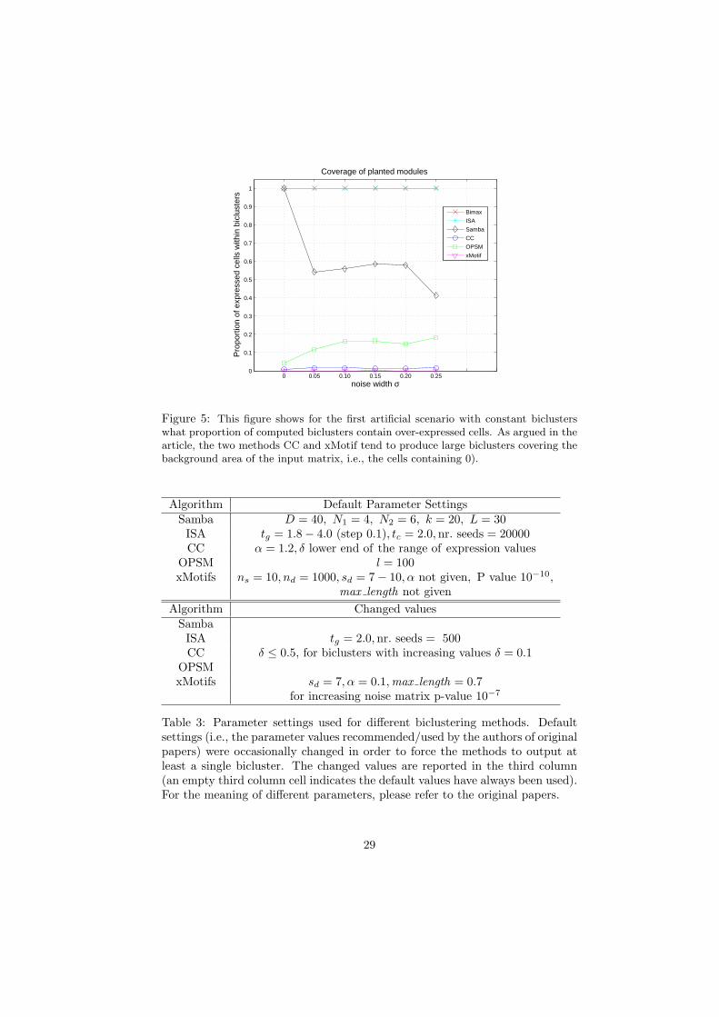
Figure 5: This figure shows for the first artificial scenario with constant biclusterswhat proportion of computed biclusters contain over-expressed cells. As argued in thearticle, the two methods CC and xMotif tend to produce large biclusters covering thebackground area of the input matrix, i.e., the cells containing 0).

Algorithm Default Parameter SettingsSamba D = 40, N1 = 4, N2 = 6, k = 20, L = 30ISA tg = 1.8− 4.0 (step 0.1), tc = 2.0,nr. seeds = 20000CC α = 1.2, δ lower end of the range of expression values

OPSM l = 100xMotifs ns = 10, nd = 1000, sd = 7− 10, α not given, P value 10−10,

max length not given

Algorithm Changed valuesSambaISA tg = 2.0,nr. seeds = 500CC δ ≤ 0.5, for biclusters with increasing values δ = 0.1

OPSMxMotifs sd = 7, α = 0.1,max length = 0.7

for increasing noise matrix p-value 10−7

Table 3: Parameter settings used for different biclustering methods. Defaultsettings (i.e., the parameter values recommended/used by the authors of originalpapers) were occasionally changed in order to force the methods to output atleast a single bicluster. The changed values are reported in the third column(an empty third column cell indicates the default values have always been used).For the meaning of different parameters, please refer to the original papers.

29

0 1 2 3 4 5 6 7 8 90

0.1

0.2

0.3

0.4

0.5

0.6

0.7

0.8

0.9

1

1.0

1.0

1.01.0

1.0

1.0

1.0

1.0

1.2

1.2 1.2

1.2

1.21.2 1.2 1.2

1.4

1.4 1.4 1.4

1.4

1.4 1.4

1.4

1.6

1.6

1.6 1.6 1.6 1.61.6 1.6

1.8

1.8

1.81.8

1.81.8

1.81.8

2.02.0

2.0

2.0

2.0

2.0

2.0

2.0

2.2

2.2

2.2

2.2

2.2

2.2

2.2

2.2

2.4

2.4

2.4

2.4

2.4

2.42.4

2.4

Variability of ISA results; (tc, t

g) parameters

regulatory complexity

avg

mat

ch s

core

(a)

0 1 2 3 4 5 6 7 8 90

0.1

0.2

0.3

0.4

0.5

0.6

0.7

0.8

0.9

1

Variability of ISA results; (tc, t

g) parameters

regulatory complexity

avg

mat

ch s

core

(b)

0 1 2 3 4 5 6 7 8 90

0.1

0.2

0.3

0.4

0.5

0.6

0.7

0.8

0.9

1

1

1 1 1 1 1 1 1

2

22

2 22 2 2

3

33

33

3 3 3

9

99

99

9 99

10

10

1010

1010

10 10

20

20

20 2020

2020

2030

30

30

30

30

30

30

30

40

40

40

40

40

40

40

40

50

50

50

50

Variability of MK results; seed parameter

regulatory complexity

avg

mat

ch s

core

(c)

0 1 2 3 4 5 6 7 8 90

0.1

0.2

0.3

0.4

0.5

0.6

0.7

0.8

0.9

1

Variability of MK results; seed parameter

regulatory complexity

avg

mat

ch s

core

10

10

1010

1010

10 10

40

40

40

40

40

40

40

40

(d)

0 1 2 3 4 5 6 7 8 90

0.1

0.2

0.3

0.4

0.5

0.6

0.7

0.8

0.9

1

0

00

0

0

0

0

0

1.0

1.0 1.0 1.0 1.0 1.0 1.0 1.0

0.1

0.1 0.1 0.1 0.1 0.1

0.1 0.1

0.01

0.010.01

0.01

0.01

0.01

0.01

0.01

e−03

e−03

e−03

e−03

e−03

e−03

e−03

e−03

e−04

e−04 e−04

e−04

e−04

e−04

e−04

e−04

e−05

e−05 e−05

e−05

e−05

e−05

e−05e−05

e−06

e−06 e−06

e−06

e−06

e−06

e−06

e−06

e−07

e−07

e−07

e−07

e−07

e−07

e−07

e−07

e−08

e−08e−08

e−08

e−08

e−08

e−08

e−08

Variability of CC results; δ parameter

regulatory complexity

avg

mat

ch s

core

(e)

0 1 2 3 4 5 6 7 8 90

0.1

0.2

0.3

0.4

0.5

0.6

0.7

0.8

0.9

1

Variability of CC results; δ parameter

regulatory complexity

avg

mat

ch s

core

(f)

Figure 6: Variability of the average bicluster relevance score depending on the pa-rameter settings (constant biclusters). The plotted values represent averages over thebiclusters obtained by ISA, xMotif and CC. (a), (b): For ISA, we varied the (tg, tc)parameters, in all cases, tg = tc, with 1.0 ≤ tg ≤ 2.4; the value recommended byauthors is (2.0, 2.0). (c), (d): As to xMotif, the size of the random seeds was changedin the range 1 − 50; values recommended by the authors are in the range 7 − 10. (e),(f): For CC, the homogeneity threshold, δ, has been systematically varied; the redbold line in (e) shows the results obtained for δ = 0, i.e., when only perfect biclustersare sought.

30