Comparison Between Stress Analysis in a Siemens SolidEdge/Nx-Nastran and p-adaptive Analysis using

StressRefineTM

Richard B KingFounder & Principal

StressRefine, Inc

Executive Summary

Accurate and adaptive stress analysis, with minimal user intervention, is crucial for engineers who are not specialists in analysis. These users represent a large potential market for structural simulation products.

Siemens SolidEdge/Nx-Nastran (NX) provides easy to use stress analysis capability targeted for design engineers. But to obtain accurate stress results, it is often necessary for considerable user intervention, in adjusting mesh settings, defining local mesh controls, etc. This makes it difficult for the target users to get good results.

StressRefine (SR) is a new technology which uses adaptive-p finite element analysis for accurate stress analysis. StressRefine is the result of man-years of development by one of the original founders of the Rasna Mechanica simulation products who undertook to extend current simulation analysis approaches into new areas upon leaving PTC.

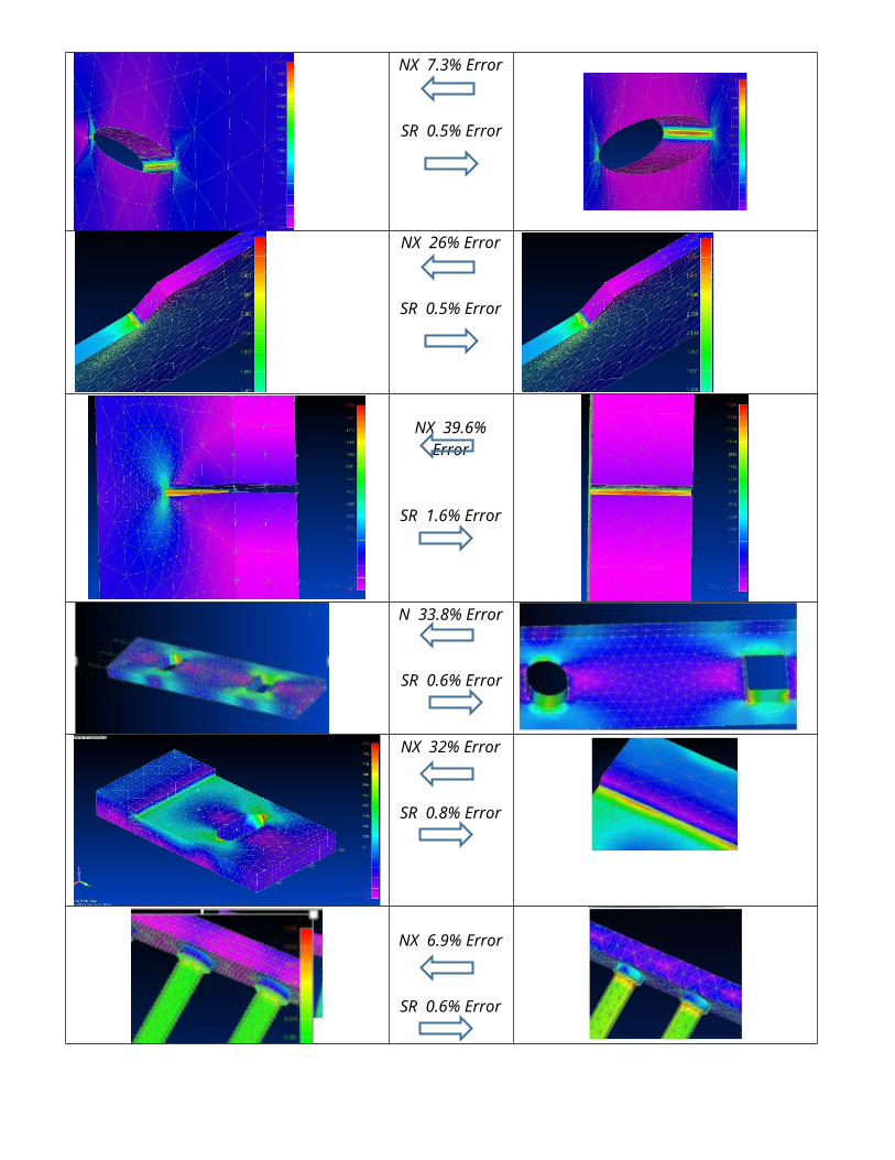
In the study described below and summarized in Fig. 1, in multiple cases with stress concentrations, the NX results were inaccurate with FEMAP default mesh settings. In almost all cases these results look qualitatively reasonable so would be likely to be accepted by design engineers as correct. Running the same models in FEMAP with adaptive meshing also led to inaccurate stresses in several of the cases. SR achieved accurate results on all these cases using the default meshes from FEMAP. The run times for SR were comparable to the adaptive run times in FEMAP.

This study shows that p-adaptive analysis with quadratic mapping works well on typical default meshes from NX. SR is a useful addition to Solidedge/NX for use by design engineers, providing fast and accurate results automatically

NX 7.3% Error

SR 0.5% Error

NX 26% Error

SR 0.5% Error

NX 39.6% Error

SR 1.6% Error

N 33.8% Error

SR 0.6% Error

NX 32% Error

SR 0.8% Error

NX 6.9% Error

SR 0.6% Error

NX 45% Error

SR 2.2% Error

NX 32.6% Error

SR 2.4% Error

Figure 1. Summary of Comparison of results with default mesh in NX (left) with StressRefine adaptive results on the same mesh (right) for various models.

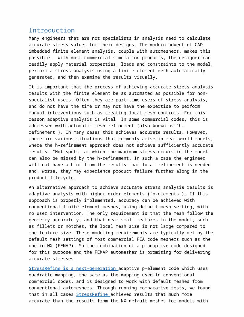
IntroductionMany engineers that are not specialists in analysis need to calculate accurate stress values for their designs. The modern advent of CAD imbedded finite element analysis, couple with automeshers, makes this possible. With most commercial simulation products, the designer can readily apply material properties, loads and constraints to the model, perform a stress analysis using a finite element mesh automatically generated, and then examine the results visually.

It is important that the process of achieving accurate stress analysis results with the finite element be as automated as possible for non-specialist users. Often they are part-time users of stress analysis, and do not have the time or may not have the expertise to perform manual interventions such as creating local mesh controls. For this reason adaptive analysis is vital. In some commercial codes, this is addressed with automatic mesh refinement (also known as “h-refinement”). In many cases this achieves accurate results. However, there are various situations that commonly arise in real-world models, where the h-refinement approach does not achieve sufficiently accurate results. “Hot spots” at which the maximum stress occurs in the model can also be missed by the h-refinement. In such a case the engineer will not have a hint from the results that local refinement is needed and, worse, they may experience product failure further along in the product lifecycle.

An alternative approach to achieve accurate stress analysis results is adaptive analysis with higher order elements (“p-elements”). If this approach is properly implemented, accuracy can be achieved with conventional finite element meshes, using default mesh setting, with no user intervention. The only requirement is that the mesh follow the geometry accurately, and that near small features in the model, such as fillets or notches, the local mesh size is not large compared to the feature size. These modeling requirements are typically met by the default mesh settings of most commercial FEA code meshers such as the one in NX (FEMAP). So the combination of a p-adaptive code designed for this purpose and the FEMAP automesher is promising for delivering accurate stresses.

StressRefine is a next-generation adaptive p-element code which uses quadratic mapping, the same as the mapping used in conventional commercial codes, and is designed to work with default meshes from conventional automeshers. Through running comparative tests, we found that in all cases StressRefine achieved results that much more accurate than the results from the NX default meshes for models with stress concentrations that are typical of real-world scenarios. StressRefine also achieved significantly more accurate results even compared to meshes that had been refined the amount one could reasonably expect from a non-expert user. The only prerequisite for accuracy using the technology in StressRefine is that the mesh follow curved geometry correctly, and that the elements not be large in comparison to the size of small features where stress concentrations occur. This criterion was typically met by the FEMAP mesher with default settings.

Detailed Investigation of Stress Accuracy with conventional FEA using NX, and p-adaptivity using SR

A variety of models were analyzed with NX using default mesh settings (but with “midside nodes on surfaces” and “curvature-based mesh refinement” always checked). It was found that with the default mesh settings, the automesher typically did a poor job of following the geometry, as shown in appendix 3. The stress results for these meshes were alos very inaccurate. If the same models were imported in FEMAP and meshed with the same default settings, a much better mesh resulted. For this reason the results from the FEMAP default meshes were used in this study. For comparison, the exact same mesh was run in StressRefine. Where theoretical results were available these were used to judge the accuracy of results. Otherwise the model was manually remeshed with successively fine mesh settings in FEMAP and the result from this very fine mesh control was used for the correct solution. There is adaptivity available in the custom tools menu in FEMAP, so I also compared the adaptive mesh results from FEMAP with the StressRefine results.

The results from SR were imported back into FEMAP in Nastran format for display. The FEMAP postprocessor linear interpolates between stress values at the corners of elements. This loses accuracy for higher order elements. For this reason SR overlays a finer grid on the actual mesh before exporting results so that stresses can be sampled more precisely. This finer grid is what appears in the figures, the actual mesh used was identical to the default mesh from FEMAP. This is discussed and illustrated with a figure in appendix 4.

For some simple models, theoretical results are available to check the accuracy of finite element results. For more complicated models with no theoretical comparison, an accurate result was achieved by manually refining the NX model multiple times, through global mesh settings and local mesh controls, until a converged result was obtained. For all the results presented below, unless otherwise noted, “Stress” refers to von Mises Stress.

First we analyzed 2 simpler models for which a theoretical solution is available, and NX and SR both achieved accurate and smooth results. These are shown in the figures 2, and 3 and the results tabulated in table 1. These preliminary results give confidence in the comparison between the two codes. These are typical models

Fig. 2 Thick Sphere under pressure. NX result with default mesh (a), SR result (b)

Fig. 3. Plate with hole under tension. NX result with default mesh (a), SR result (b)

Sharp Stress Concentration- elliptical holeNext we investigated a series of models with sharper stress concentrations which present challenges for conventional FEA. The first is a plate with a narrow elliptical hole (aspect ratio 4 to 1) (fig. 4). This is more difficult because there is a small sharply curved feature. The theoretical stress-YY in an infinite plate is 9 times the applied stress. Since a large but finite width plate was analyzed, a result of about 10% higher is expected. Stress YY is the same a maximum principal stress at the point of max stress. A highly refined NX mesh for this model gave the anticipated result of 9.93 for maximum principal stress. The NX result with the default FEMAP mesh for this model was 9.2, or in error by 7.3 Using adaptive meshing (custom tools/postprocessing/tetra adaptive mesh and rerun) resultied in as stress of 9.59 (error 3.4%). Using the default mesh in SR, the result was in a maximum stress-YY of 9.95, in agreement within 0.2% with the control results. For this model adaptive remeshing in FEMAP achieved accurate results. That was not found to be true in several other models examined below.

Fig. 4. Plate with elliptical hole under tension. Result with NX default mesh (a), FEMAP result with adaptive mesh (b), SR result (c)

Stepped Flat Bar With Shoulder Fillets in TensionThe next model was a stepped bar with shoulder fillets subject to tension (Fig. 5). The theoretical result for this case is 3.3. The NX result with default mesh was 2.45, in error by 26%. Using FEMAP adaptive meshing gave the same result. The SR result was 3.27, in error by 0.8%.

Fig. 5 Stepped bar with fillet. Result with NX default mesh (a), FEMAP result with adaptive mesh (b), SR result (c)

Thin notchThe next model was a plate under tension with a thin notch (fig. 6), modeled with half-symmetry. The very fine mesh control result for this case was 12.9. The NX result with default mesh was 7.79, in error by 39.6%. Using FEMAP adaptive meshing made the result worse: 6.74, in error by 47.7%. The SR result was 13.09, in error by 1.6%.

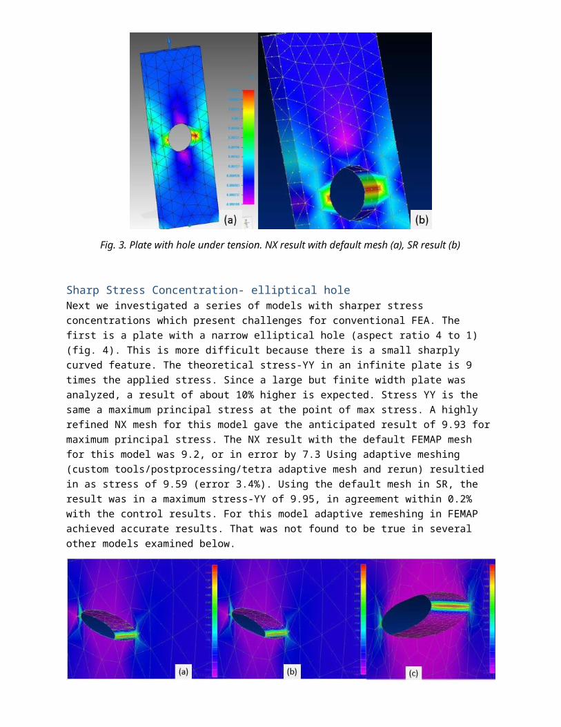
Fig.6. Model with thin notch under tension. Result with NX default mesh (a) and (b), FEMAP result with adaptive mesh (c), SR result (d)

Models with More than one Stress Concentration

The next model shows the difficulty when there are more than one stress concentrations, and it is possible for h-refinement to miss the hot-spot where the maximum stress in the model occurs. In this model, there is both a hole in a thinner section of the model, and a sharp fillet between thinner and thicker sections. From the analysis with default mesh, it appears that the maximum stress is at the hole. So a user refining the mesh would be inclined to put surface mesh controls at the hole but not at the fillet.

A very fine mesh control in NX shows that the maximum stress in the model is 9, at the fillet. The default NX mesh predicts the maximum stress in the model to be 8.2, at the hole. At the fillet it predicts a stress of 6.01, which is 32% low, and the results are not smooth. The refined mesh in NX gives a value of 6.2 at the fillet, in error by 31%. Using adaptive made the results worse, resulting in as stress of 5.2 (error 42%). The SR result was 9.22, in error by 2.4%.

Fig.7. Stepped Model under tension. Result with FEMAP/NX default mesh (a) and (b), FEMAP result with adaptive mesh (c), SR result (d)

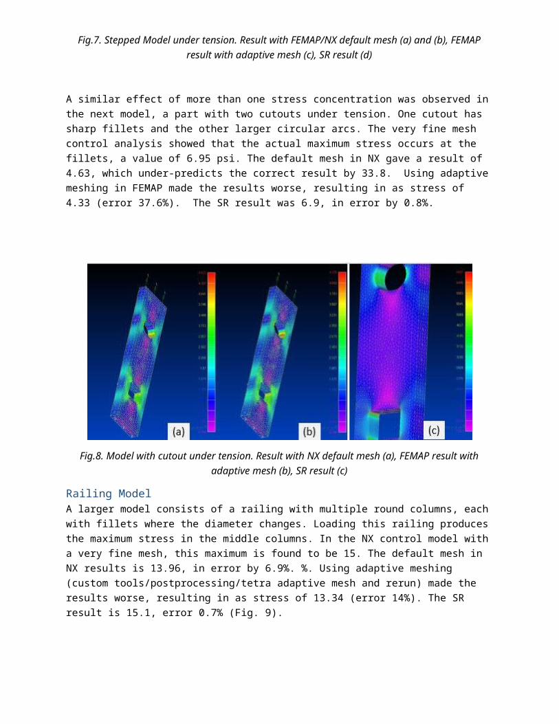
A similar effect of more than one stress concentration was observed in the next model, a part with two cutouts under tension. One cutout has sharp fillets and the other larger circular arcs. The very fine mesh control analysis showed that the actual maximum stress occurs at the fillets, a value of 6.95 psi. The default mesh in NX gave a result of 4.63, which under-predicts the correct result by 33.8. Using adaptive

meshing in FEMAP made the results worse, resulting in as stress of 4.33 (error 37.6%). The SR result was 6.9, in error by 0.8%.

Fig.8. Model with cutout under tension. Result with NX default mesh (a), FEMAP result with adaptive mesh (b), SR result (c)

Railing ModelA larger model consists of a railing with multiple round columns, each with fillets where the diameter changes. Loading this railing produces the maximum stress in the middle columns. In the NX control model with a very fine mesh, this maximum is found to be 15. The default mesh in NX results is 13.96, in error by 6.9%. %. Using adaptive meshing (custom tools/postprocessing/tetra adaptive mesh and rerun) made the results worse, resulting in as stress of 13.34 (error 14%). The SR result is 15.1, error 0.7% (Fig. 9).

Fig.9. Railing Model. Result with NX default mesh (a), FEMAP result with adaptive mesh (b, SR result (c)

Thin Solid ModelThe next model was a 3D solid with a thin cantilevered section. There is a fillet at the transition between the thick and thin sections. The fine mesh control for this model requires a large number of tetrahedral elements to achieve a converged result for stress. The maximum stress for this control model is 6.26, at

the fillet. The default result from NX is 3.43, in error by 45%, and the result for adaptive meshing in FEMAP was 4.97, in error by 21%. The result from SR is 6.12, a 2.2% error.

Fig. 10. Model with thin cantilever section. Result with NX default mesh (a FEMAP result with adaptive mesh (b), SR result (c)

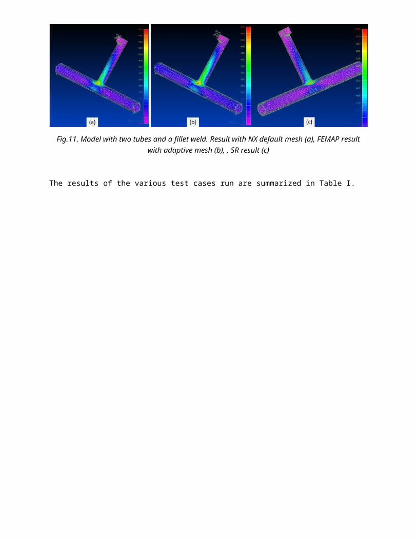
Welded Tube ModelThe final model examined was two tubes welded together with a fillet weld. Using a very fine mesh control in NX gives a value of 10.3 for the max stress. The default mesh result from NX is 6.94, in error by 32.6%, and the FEMAP adaptive meshing result is 6.05, in error by 41.3%.

Fig.11. Model with two tubes and a fillet weld. Result with NX default mesh (a), FEMAP result with adaptive mesh (b), , SR result (c)

The results of the various test cases run are summarized in Table I.

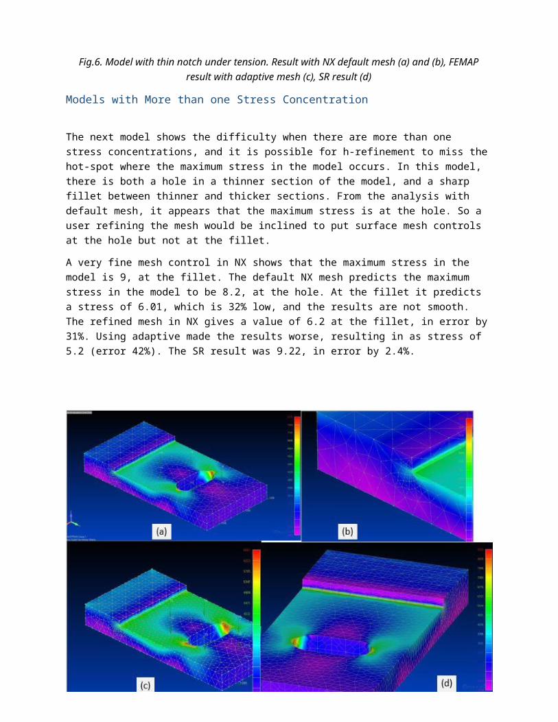
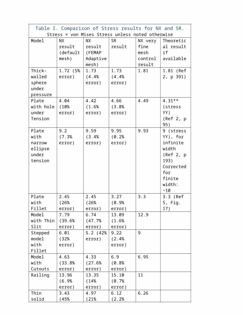
Table I. Comparison of Stress results for NX and SR.Stress = von Mises Stress unless noted otherwise

Model NX result (default mesh)

NX result (FEMAPAdaptive mesh)

SR result NX very fine mesh control result

Theoretical result if available

Thick-walled sphere under pressure

1.72 (5% error)

1.73 (4.4% error)

1.73 (4.4% error)

1.81 1.81 (Ref 2, p 391)

Plate with hole under Tension

4.04 (10% error)

4.42 (1.6% error)

4.66 (3.8% error)

4.49 4.31** (stress YY)(Ref 2, p 95)

Plate with narrow ellipse under tension

9.2 (7.3% error)

9.59 (3.4% error)

9.95 (0.2% error)

9.93 9 (stress YY), for infinite width (Ref 2, p 193)Corrected for finite width: ~10

Plate with Fillet

2.45 (26% error)

2.45 (26% error)

3.27 (0.9% error)

3.3 3.3 (Ref 5, Fig. 17)

Model with Thin Slit

7.79 (39.6% error)

6.74 (47.7% error)

13.09 (1.6% error)

12.9

Stepped model with Fillet

6.01 (32% error)

5.2 (42% error)

9.22 (2.4% error)

9

Model with Cutouts

4.63 (33.8% error)

4.33 (27.6% error)

6.9 (0.8% error)

6.95

Railing 13.96 (6.9% error)

13.35 (14% error)

15.10 (0.7% error)

11

Thin solid model

3.43 (45% error)

4.97 (21% error)

6.12 (2.2% error)

6.26

Welded Tube Model

6.94 (32.6% error)

6.05 (41.3% error)

10.05 (2.4 % error)

10.3

** Note: The theoretical solution for the plate with hole is for plane stress, so the 3D result for finite thickness is expected to be a little higher than the theory

Table II. P-order Statistics, average of all example runs discussed. The majority of all elements remain at low order

P-order Percentage of model2 81.843 9.704 2.645 1.746 3.74

7 0.33

Appendix 1 – h vs p refinement

Uniform vs Adaptive P refinementUniform p refinement can be done with conventional isoparametric finite elements. For example, a quadratic tetrahedron will have 4 corner nodes and 6 midside nodes (one per edge). To increase the polynomial order to cubic, the 6 midside nodes are replaced with 12 (two per edge). This approach is used in some commercial codes because it is relatively straightforward to implement. Uniform p refinement is inefficient because the p-order of every element in the model must be increased.

An alternative is to use an adaptive higher order element as described in the theory section below. This allows the polynomial order of each element to be adapted independently for a much more efficient solution. Table II shows that higher polynomial orders were required at only a small fraction of the models for the cases investigated in this study. Also, conventional isoparametric finite elements become inefficient when the p order becomes high, so in practice they should not be used much higher than about p order 5. But the adaptive p elements in StressRefine remain numerically well-conditioned to much higher p orders like 10.

P refinementPros:

Adaptivity does not require remeshing Adaptivity is extremely local. Only elements with errors above tolerance need higher polynomial

orders. Stiffness matrices of unaffected elements do not need to be recalculated. Higher-order elements generally lead to smoother results for stresses.

Cons:

Becomes inefficient at very high polynomial orders. A practical limit is about p order 8. This means convergence may not be obtained if the mesh is too coarse in a region of rapid solution variation. In practice, good results are achieved if curved geometric features are accurately modelled, the elements are not too distorted in regions of stress concentration, and the element size near small features is comparable to the feature size. These requirements were readily met by the FEMAP automesher in all the cases I tried.

If higher-order mapping is used, p-elements with low p-orders can exhibit spurious rigid-body energy in some problems. This is avoided in SR which uses quadratic mapping. The elements are only used at p-order 2 and above, so they have no rigid body issues. There are other approaches to solving this issue but this is the simplest. It assumes a fine enough mesh in curved regions as discussed in the above bullet.

The p-method is more difficult to implement. All element routines have to be rewritten to use special basis functions. This is alleviated if the basis function routines are packaged modularly as in SR.

h-refinementPros:

Readily implemented with a conventional finite element code by wrapping an iterative mesh refinement loop around the finite element code.

In principal this could lead to arbitrarily accurate results, as the refinement could be continued until the mesh was very fine. In practice this is limited by performance considerations.

Cons

Stress results in regions of high stress variation may not be smooth. Adaptivity can be less local. When the mesh is refined with new seeding from error estimates,

the remeshed zone may propagate further than the zone of high error. For large models, automeshing can be difficult. Adaptive mesh refinement will fail if the model

cannot be remeshed.

Performance considerationsConvergence to a specified accuracy is typically achieved with a smaller number of equations for the p-method, which is claimed as an advantage in the literature. However, the stiffness matrices for p-adaptive solutions tend to be smaller but denser than those for h-adaptivity. So faster performance does not necessarily occur. For the models used in the detailed comparison above, the run times were comparable and quite reasonable for both NX and SR. The largest model was the railing with columns which took 24.3 seconds for mesh and solve in SR vs 18 seconds for mesh and solve for the adaptive mesh result in NX. However this is using a trial version of the Intel Mkl pardiso solver which is not running multithreaded on my machine (Intel quad core i7). The run time would be reduced considerably if 8 threads were exploited.

Another performance consideration for p-refinement is the maximum p-order to use. In my experience there is a “marginal return on investment” for increased accuracy at very high polynomial orders. For that reason a maximum p-order of about 7 or 8 is reasonable for a compromise between accuracy and run time. Maximum p of 7 was used in the analyses reported above.

SingularitiesVarious common types of modeling approximations, including defeaturing, lead to mathematical singularities, so the stress values are theoretically infinite. These singular regions include reentrant corners, certain types of partial constraints on surfaces, point and edge loads. When h or p refinement is performed in the presence of singularities, computations can be wasted producing physically meaningless results. SR handles this by automatically detecting many types of singularities. The adjacent elements are exempted from refinement, and are skipped when calculating max stress in model. The user is warned that the model theoretically has infinite stress and requested to review the model.

Higher-order adaptive p-element theoryThe theory of higher-order finite elements is described in detail in Ref. 1 and will be briefly reviewed here. The elements use different functions for mapping (“shape functions”) and displacement (“basis functions”).

The physical coordinate of a point at a natural coordinate r on an edge is

x(r) = ∑ xi Ni

where Ni are the shape functions, and the displacements are

u(r) = ∑ ui hi

where hi are the basis functions.

For conventional isoparametric finite elements the same number and type functions are used for both shape and basis, e.g. linear or quadratic “serendipity” functions (Ref. 3). For higher order p-elements, these differ in number and type. Various functions have been used for the mapping functions in previous implementations of the p-method. StressRefine uses conventional quadratic functions to assure compatibility with meshes from typical automeshers. For the basis functions, integrals of Legendre polynomials are used along edges. These lead to much better conditioned stiffness matrices for high polynomial orders than conventional polynomial functions. They are blended to form 2D functions on faces and 3D functions in elements.

There is difficulty extending to 2 and 3 dimensions when using higher order basis functions with arbitrary polynomial order on any edge. The orientation of element local edges and faces compared to global model edges and faces must be properly considered to ensure continuity of basis functions across element boundaries. This is tricky to code but not computationally intensive. Once the 3 dimensional basis function library is available, however, it is readily integrated into any element routine. The basis library in SR is modular and easily called.

A major advantage of the higher order p-method for adaptivity is that a different polynomial order can be specified on each edge of the model, which allows adjacent elements to have different orders as is illustrated for a simple 2D case in Fig. 12. This makes arbitrary adaptivity easy to implement. Given local error measures, polynomial orders can be adjusted as needed. This is illustrated in table II, which shows that for the models described in this study, most of the model stays at low polynomial order.

Error estimation for p-adaptivity is similar to that for h-adaptivity. For example, stress errors can be assessed using the type of estimators described in ref 4. Instead of using these to estimate a required element size, they are used to estimate an appropriate polynomial order.

With the availability of a basis function library such as in SR, it is straightforward to convert existing quadratic h elements to adaptive p elements. The h-shape functions are retained for mapping, but for displacement gradient calculations they are replaced with the p-basis functions.

Figure 12. Independent adjustment of polynomial orders of adjacent adaptive P elements.

Appendix 2 – StressRefine Capabilities Linear Statics. Brick, tetrahedral, and wedge higher order elements (p 2 to 8) with quadratic mapping. Robust transition elements for assembling to conventional finite element meshes p-Adaptive refinement with variable number of iterations and user-specified error tolerance. Global stress smoothing (“superconvergent” stress recovery). Loading includes nodal, edge, and face forces, pressure, thermal, gravity, centrifugal, and

enforced displacement in user-specified coordinate systems (Cartesian, cylindrical, or spherical). Higher-order basis function library: modular and readily integrated into element routines in

other codes. Detailed singularity detection Uses Intel Mkl Pardiso sparse solver. Automatic singularity detection and exclusion, and warning. Thin element detection for high aspect ratio bricks and wedges. Isotropic and Anisotropic materials. Readily extendable to modal analysis.

Appendix 3- SolidEdge vs FEMAP default mesh

Figure 13. Part with elliptical hole. Mesh From SolidEdge NX (a) and (b), Mesh from FEMAP (c)

The meshes produced with the default settings in SolidEdge NX did a poor job of following geometry as shown in Figure 13. This is with the same default settings as in FEMAP. These meshes led to inaccurate results for stress as shown in Fig. 14. But if the models were imported into FEMAP and meshed there, meshes that followed the geometry well resulted. This is odd because SolidEdge NX uses the FEMAP mesher. These were models created in a different CAD package and imported as parasolid binary (.x_b). There may have been a scaling issue in SolidEdge. Since the FEMAP meshes followed the geometry well, these meshes were used for the StressRefine runs and for the NX results to compare with SR in this study.

NX 79% Error

SR 0.5% Error

NX 36% Error

SR 1.6% Error

NX 39% Error

SR 0.6% Error

NX 39% Error

SR 0.8% Error

NX 20% Error

SR 0.6% Error

NX 45% Error

SR 2.2% Error

NX 37% Error

SR 2.4% Error

Figure 41. Summary of Comparison of results with default mesh in NX, using default mesh settings in Solidedge (left) with StressRefine adaptive results on the same mesh (right) for various models.

Appendix 4- Refined Grid for postprocessingConventional postprocessors, such as the one in NX and FEMAP, linearly interpolate between stress values at the corners of elements. For higher order elements, the stress can vary much more sharply than this, and accuracy is lost by linearly interpolating, especially in the vicinity of stress concentrations. SR overcomes this limitation by overlaying a finer grid (e.g. by replacing each tetrahedron with 4 bricks) on the actual mesh before exporting results, so that stresses can be sampled more precisely. An example of this is shown in Figure 14. On the left is the actual mesh used to analyze the welded tube model, while on the right is the finer grid for postprocessing.

Figure 15. Welded tube model. Coarse mesh used for analysis (a), and fine grid for postprocessing (b).

References1. Szabo, B, and Babusca, I, Finite Element Analysis, Wiley, NY, 19912. Timoshenko, S, and Goodier, J, Theory of Elasticity, McGraw-Hill, NY, 1970.3. Zienkiewicz, O, and Taylor, R, The Finite Element Method, Butterworth Heinemann, Oxford,

2000.4. Zienkiewicz, O, and Zhu, J, “Superconvergent Patch Recovery and a posteriori error estimation in

the finite element method”, Int. J. Num. Meth. Engr, 33, 1331, 1992.5. Peterson, R, Stress Concentration Factors, Wiley, NY, 1974.