Comparison between SMOS, VUA, ASCAT, and ECMWF soil ...
21
HAL Id: ird-00828830 http://hal.ird.fr/ird-00828830 Submitted on 31 May 2013 HAL is a multi-disciplinary open access archive for the deposit and dissemination of sci- entific research documents, whether they are pub- lished or not. The documents may come from teaching and research institutions in France or abroad, or from public or private research centers. L’archive ouverte pluridisciplinaire HAL, est destinée au dépôt et à la diffusion de documents scientifiques de niveau recherche, publiés ou non, émanant des établissements d’enseignement et de recherche français ou étrangers, des laboratoires publics ou privés. Comparison between SMOS, VUA, ASCAT, and ECMWF soil moisture products over four watersheds in U.S. D. Leroux, Y.H. Kerr, A. Albitar, R. Bindlish, T.J. Jackson, B. Berthelot, G. Portet To cite this version: D. Leroux, Y.H. Kerr, A. Albitar, R. Bindlish, T.J. Jackson, et al.. Comparison between SMOS, VUA, ASCAT, and ECMWF soil moisture products over four watersheds in U.S.. IEEE Transactions on Geoscience and Remote Sensing, Institute of Electrical and Electronics Engineers, 2013, pp.1-20. <10.1109/TGRS.2013.2252468>. <ird-00828830>
Transcript of Comparison between SMOS, VUA, ASCAT, and ECMWF soil ...
HAL Id: ird-00828830http://hal.ird.fr/ird-00828830
Submitted on 31 May 2013
HAL is a multi-disciplinary open accessarchive for the deposit and dissemination of sci-entific research documents, whether they are pub-lished or not. The documents may come fromteaching and research institutions in France orabroad, or from public or private research centers.
L’archive ouverte pluridisciplinaire HAL, estdestinée au dépôt et à la diffusion de documentsscientifiques de niveau recherche, publiés ou non,émanant des établissements d’enseignement et derecherche français ou étrangers, des laboratoirespublics ou privés.
Comparison between SMOS, VUA, ASCAT, andECMWF soil moisture products over four watersheds in
U.S.D. Leroux, Y.H. Kerr, A. Albitar, R. Bindlish, T.J. Jackson, B. Berthelot, G.
Portet
To cite this version:D. Leroux, Y.H. Kerr, A. Albitar, R. Bindlish, T.J. Jackson, et al.. Comparison between SMOS,VUA, ASCAT, and ECMWF soil moisture products over four watersheds in U.S.. IEEE Transactionson Geoscience and Remote Sensing, Institute of Electrical and Electronics Engineers, 2013, pp.1-20.<10.1109/TGRS.2013.2252468>. <ird-00828830>
IEEE
Proo
f
IEEE TRANSACTIONS ON GEOSCIENCE AND REMOTE SENSING 1
Comparison Between SMOS, VUA, ASCAT, andECMWF Soil Moisture Products Over Four
Watersheds in U.S.DELPHINE J. Leroux, Yann H. Kerr, Fellow, IEEE, Ahmad Al Bitar, Rajat Bindlish, Senior Member, IEEE,
Thomas J. Jackson, Fellow, IEEE, Beatrice Berthelot, and Gautier Portet
Abstract— As part of the Soil Moisture and Ocean Salinity(SMOS) validation process, a comparison of the skills of threesatellites [SMOS, Advanced Microwave Scanning Radiometer-Earth Observing System (AMSR-E) or Advanced MicrowaveScanning Radiometer, and Advanced Scatterometer (ASCAT)],and one-model European Centre for Medium Range WeatherForecasting (ECMWF) soil moisture products is conducted overfour watersheds located in the U.S. The four products comparedin for 2010 over four soil moisture networks were used for thecalibration of AMSR-E. The results indicate that SMOS retrievalsare closest to the ground measurements with a low average rootmean square error of 0.061 m 3· m−3 for the morning overpassand 0.067 m 3· m−3 for the afternoon overpass, which representsan improvement by a factor of 2–3 compared with the otherproducts. The ECMWF product has good correlation coefficients(around 0.78) but has a constant bias of 0.1–0.2 m 3· m−3 overthe four networks. The land parameter retrieval model AMSR-Eproduct gives reasonable results in terms of correlation (around0.73) but has a variable seasonal bias over the year. The ASCATsoil moisture index is found to be very noisy and unstable.
Index Terms— Soil moisture, Soil Moisture and Ocean Salinity(SMOS), validation.
I. INTRODUCTION
SOIL moisture is an important variable in the study ofseasonal climate evolution and prediction as it plays a
major role in the mass and energy transfers between the soiland the atmosphere [1]. In land surface models, soil moistureis the key parameter in determining the evaporative fraction at
Manuscript received July 26, 2012; revised January 10, 2013; acceptedFebruary 19, 2013. This work was supported in part by Telespazio Franceand TOSCA.
D. J. Leroux is with the Centre d’Etudes Spatiales de la Biosphere,Toulouse, France and Telespazio, Toulouse 31404, France (e-mail: [email protected]).
Y. H. Kerr and A. Al Bitar are with the Centre d’Etudes Spatiales dela Biosphere, Toulouse 31404, France (e-mail: [email protected];[email protected]).
R. Bindlish and T. J. Jackson are with the U.S. Department of Agricul-ture, Agricultural Research Center Hydrology and Remote Sensing Labora-tory, Beltsville, MD 20705-2350 USA (e-mail: [email protected];[email protected]).
B. Berthelot is with Magellium, Toulouse 31520, France (e-mail: [email protected]).
G. Portet is with Telespazio, Toulouse 31023, France (e-mail: [email protected]).
Color versions of one or more of the figures in this paper are availableonline at http://ieeexplore.ieee.org.
Digital Object Identifier 10.1109/TGRS.2013.2252468
the surface and the infiltration in the root zone. Soil moistureinformation is also essential for agriculture at a local scaleand for water resources management at a regional scale. Atthe global scale, soil moisture is of great value for weatherforecasting [2], climate change [3], and monitoring extremeevents such as floods.
Recently, satellite missions specially designed for soil mois-ture monitoring are implemented (Soil Moisture and OceanSalinity (SMOS) [4]) and proposed (Soil Moisture ActivePassive (SMAP) [5]). SMOS was successfully launched bythe European Space Agency in November 2009 and SMAP isscheduled for launch in October 2014 by the National Aero-nautics and Space Administration. Both satellite instrumentsare designed to acquire data at the most suitable frequency forsoil moisture retrieval (1.4 GHz [6]).
Several approaches are developed to retrieve soil mois-ture using the higher frequencies that are the only optionuntil now. These include passive Scanning MultispectralMicrowave Radiometer (SMMR, 1978–1987 [7]), passiveSpecial Sensor Microwave/Imager (SSM/I, 1987 [7]), passiveAdvanced Microwave Scanning Radiometer-Earth ObservingSystem (AMSR-E, 2002) [7], [8], WindSat (passive instru-ment, 2003 [9]), and active Advanced Scatterometer (ASCAT,1991) [10]). Although their lowest frequencies (5–20 GHz)are not the most suitable for soil moisture retrievals becauseof their high sensitivity to the vegetation and the atmosphere,they provide valuable data since 1978.
All of the products above are obtained at a relatively coarseresolution, typically around 50 km, and relating them to pointmeasurements for validation purposes is not always straight-forward especially at a global scale. Therefore, it is necessaryto validate coarse scale soil moisture estimates with modeloutputs or in situ observations from dense networks thatrepresent area average soil moisture conditions. For SMOS,the initial validation is performed on a number of sites[11] and [12]. However, it is also necessary to compare thenew SMOS product to already existing products. Here, we usealternative satellite products and outputs from a model-basedsystem. We use in situ data to establish the performance andreliability of each product.
The following section describes the comparison ofthe four soil moisture data sets over four watersheds.The methodology used is described in Section III. Resultsfrom the comparison with ground measurements are analyzed
0196-2892/$31.00 © 2013 IEEE
IEEE
Proo
f
2 IEEE TRANSACTIONS ON GEOSCIENCE AND REMOTE SENSING
in Section IV. Finally, some conclusions are summarized inthe last section.
II. DATA
A. Satellite-Based Soil Moisture Products
1) SMOS: The SMOS [4] satellite was launched in Novem-ber 2009. This is the first satellite specially dedicated tosoil moisture retrieval with an L-band passive radiometer(1.4 GHz [6]). SMOS provides global coverage in less thanthree days with a 43-km resolution. The satellite is polarorbiting with equator crossing times of 6:00 A.M. [local solartime (LST), ascending] and 6:00 P.M. (LST, descending). It isassumed that at L-band the signal is mainly influenced by thesoil moisture contained in the first 5 cm of the soil on averageover low vegetated areas.
SMOS acquires brightness temperatures at multiple inci-dence angles, from 0° to 55° with full-polarization mode.The angular signature is a key element of the algorithmthat retrieves the soil moisture and the vegetation opticaldepth, which expresses the quantity of signal that is absorbedby the vegetation layer, through the minimization of a costfunction between modeled (L-band microwave emission ofthe biosphere model [13]) and acquired brightness tempera-tures [14]. The novelty of the SMOS algorithm is that theheterogeneity inside the field of view of the radiometer isconsidered. Around each node of the SMOS grid, an extendedgrid of 123×123 km at a 4-km resolution, called the workingarea, is defined to quantify the heterogeneity seen by theradiometer. Each working area node belongs to one of the tenfollowing landcover classes (aggregated from ECOCLIMAPlandcover ecosystems, [15]): vegetation, forest, wetland, salinewater, fresh water, barren, permanent ice, urban area, frost,and snow. In the SMOS algorithm, a specific radiative transfermodel is associated with each class and it is thus possible toquantify the contribution of each of these classes. Consideringthe antenna pattern of the instrument, a weighting function isapplied. The soil moisture and the vegetation optical depth arethen retrieved over the relevant fractions, i.e., vegetated areasand forest (e.g., no retrieval is performed if the main classis waterbody). More information can be found in [14] and inthe algorithm theoretical basis document [16]. These retrievalproducts are known as level 2 products [14] and are availableon the icosahedral snyder equal area (ISEA)-4h9 grid, [17].The nodes of this grid are equally spaced at 15 km. In thispaper, the SMOS products used came from the reprocessingcampaign using the version 5.01 of the level 2 soil moistureprocessor.
2) ASCAT: The ASCAT was launched in October 2006 onthe MetOp-A satellite as a follow-on to the European RemoteSensing (ERS) satellites with the SCAT scatterometer thatstarted operating in 1991. Since its launch, it is acquiring dataat C-band (5.3 GHz). The scatterometer is composed of sixbeams: three on each side of the satellite track with azimuthangles of 45°, 90°, and 135° azimuth angles (incidence anglesare in a range of 25°–64°), which generates two swaths of550 km each with a spatial resolution of 25 or 50 km. Thecrossing times are 9:30 P.M. LST for the ascending orbit and9:30 A.M. LST for the descending orbit.
In this paper, the ASCAT 25-km soil moisture product isdownloaded from the Eumetsat data center and retrieval isperformed using the Technische Universität Wien soil moisturealgorithm [10], [18] that uses wet and dry references from theERS satellites between 1992 and 2007 to retrieve an indexranging from 0 (dry) to 1 (wet) that represents the relativesoil moisture of the first 2 cm of the soil.
3) AMSR-E: The AMSR-E was launched in June 2002on the Aqua satellite and stopped producing data in Octo-ber 2011. This radiometer acquired data with a single 55°incidence angle at six different frequencies: 6.9, 10.7, 18.7,23.8, 36.5, and 89.0 GHz, all dual polarized. The cross-ing times are 1:30 A.M. (LST, descending) and 1:30 P.M.(LST, ascending). The footprint of the antenna is around43 × 75 km at 6.9 GHz and 29 × 51 km at 10.7 GHz witha spatial resolution of 60 km at 6.9 GHz and 50 km at10.7 GHz [19].
There are several products available that used AMSR-E datato estimate soil moisture. Many studies already shown thatthe official product from the National Snow and Ice DataCenter is not able to reproduce low values of soil moisture[20]–[23]. The soil moisture product from the Vrije Univer-sity of Amsterdam (VUA) [7] is therefore chosen in thispaper.
The land parameter retrieval model [7] from the VUAretrieves the soil moisture and the vegetation optical depthusing the combination of the C- and X-band AMSR-E chan-nels and the 36.5-GHz channel to estimate the surface temper-ature. X-band observations are used in the areas of the worldwhere C-band observations are affected by radio frequencyinterferences (RFIs). This algorithm is based on a microwaveradiative transfer model with a priori information about soilcharacteristics. The operational VUA product is available ona 0.25° grid only for the descending orbit. The distributeddata over this grid are quality checked and the data that areflagged are filtered out because of high topography or extremeweather conditions, such as snow, that would decrease theobserved brightness temperatures and result in higher soilmoisture estimates. The VUA product used in this paper isthe version 3 product.
B. Model-Based Soil Moisture Product European Centrefor Medium Range Weather Forecasting (ECMWF)
The ECMWF provides medium range global fore-casts and this process produces some environmental vari-ables that include soil temperature, evaporation, and soilmoisture.
The SMOS level 2 processor uses a custom made climatedata product from ECMWF that is used to set the initial valuesin the cost function solution and to model the contributionsto the signal of the different parts of the scene seen by theradiometer. This is a forecast product generated 3–15 h inadvance and every 3 h (at 3:00 A.M., 6:00 A.M., 9:00 A.M.,and so on). It is considered an internal SMOS product as it isinterpolated at SMOS overpass times and over the SMOS grid.Thus, this custom ECMWF product has the same spatial andtemporal resolutions as SMOS and will be used in this paper.
IEEE
Proo
f
LEROUX et al.: COMPARISON BETWEEN SMOS, VUA, ASCAT, AND ECMWF SOIL MOISTURE PRODUCTS 3
The ECMWF soil moisture represents the top 7 cm below thesurface.
ECMWWF auxiliary product information can be foundin [4], [14], or [16].
C. In Situ Measurements
Four watersheds located in the United States are selectedfor this paper: Walnut Gulch (WG) in Arizona, Little Washita(LW) in Oklahoma, Little River (LR) in Georgia, and ReynoldsCreeks in Idaho. They represent different types of climate(from semiarid to humid) and land use and are in operationsince 2002 [24].
WG is located in southeast Arizona. Most of this watershedis covered by shrubs and grass, which is typical of the region.The annual mean temperature is 17.6 °C at Tombstone andthe annual mean precipitation is 320 mm, mainly from highintensity convective thunderstorms in the late summer. Theupper most 10 cm of the soil profile contains up to 60% graveland the underlying horizons usually contains less than 40%gravels.
LW is located in southwest Oklahoma in the southern GreatPlains region of the U.S. The climate is subhumid with anaverage annual rainfall of 750 mm, which falls mainly duringthe spring and fall seasons. Topography is moderately rollingwith a maximum relief of less than 200 m and land use isdominated by rangeland and pasture (63%).
LR is located in southern Georgia near Tifton. With anaverage annual precipitation of 1200 mm, the climate ishumid. This watershed is typical of the heavily vegetatedslow-moving stream systems in the coastal plain region ofthe U.S. The topography over this watershed is relatively flat.Approximately 40% of the watershed is forest with 40% cropsand 15% pasture.
RC is located in a mountainous area of southwest Idaho. Thetopography is high with a relief of over 1000 m that results indiverse climates, soils, and vegetation typical of this part ofthe Rocky Mountains. The climate is considered to be semiaridwith an annual precipitation of 500 mm. Approximately 75%of the annual precipitation at high elevation is snow whereasonly 25% is snow at low elevation.
Surface soil moisture and temperature sensors (0–5 cm) areacquiring data since 2002 for the four watersheds. The dataused in this paper are the averages of the sensors locatedin each watershed (with the weighting coefficients derivedfrom a Thiessen polygon). These averages are based on thesame sets of sensors from 2002. The in situ soil moisturedata set was distributed for the period of 2001–2011 andbecause of a significant change in the station configuration in2005–2006, only a limited number of stations is consid-ered reliable for the entire period (14/8/8/15 sensors forWG/LW/LR/RC, respectively). Therefore, even though weonly use the 2010 data in this paper, only data from thestations considered reliable for the entire period are used.In addition, several sensors are disregarded because of poor orsuspicious performances as follows: 1) sensors with periods ofmissing data are removed and only locations with continuousdata are used in the analysis; 2) the sensors are calibrated and
(a)
(b)
(c)
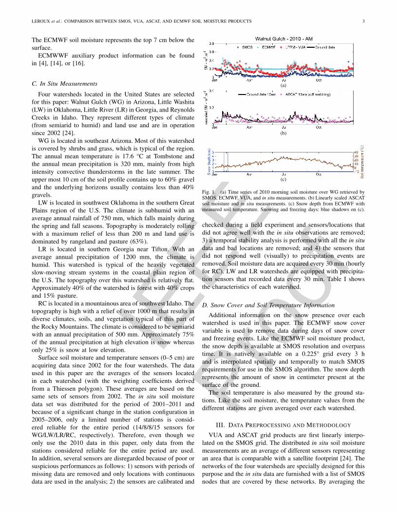
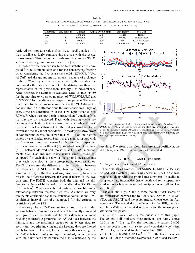
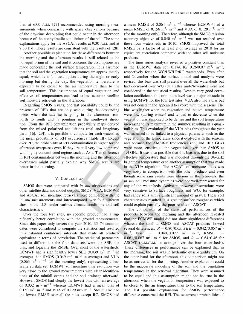
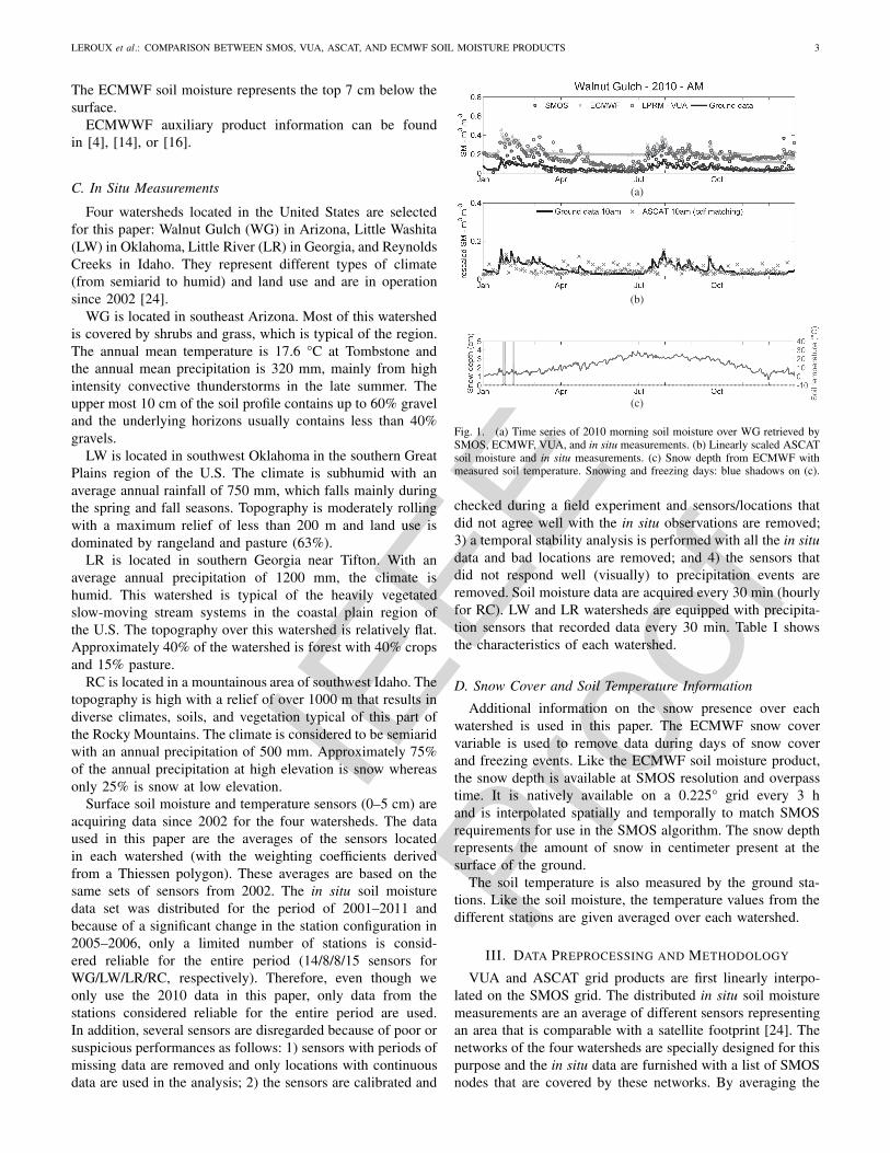
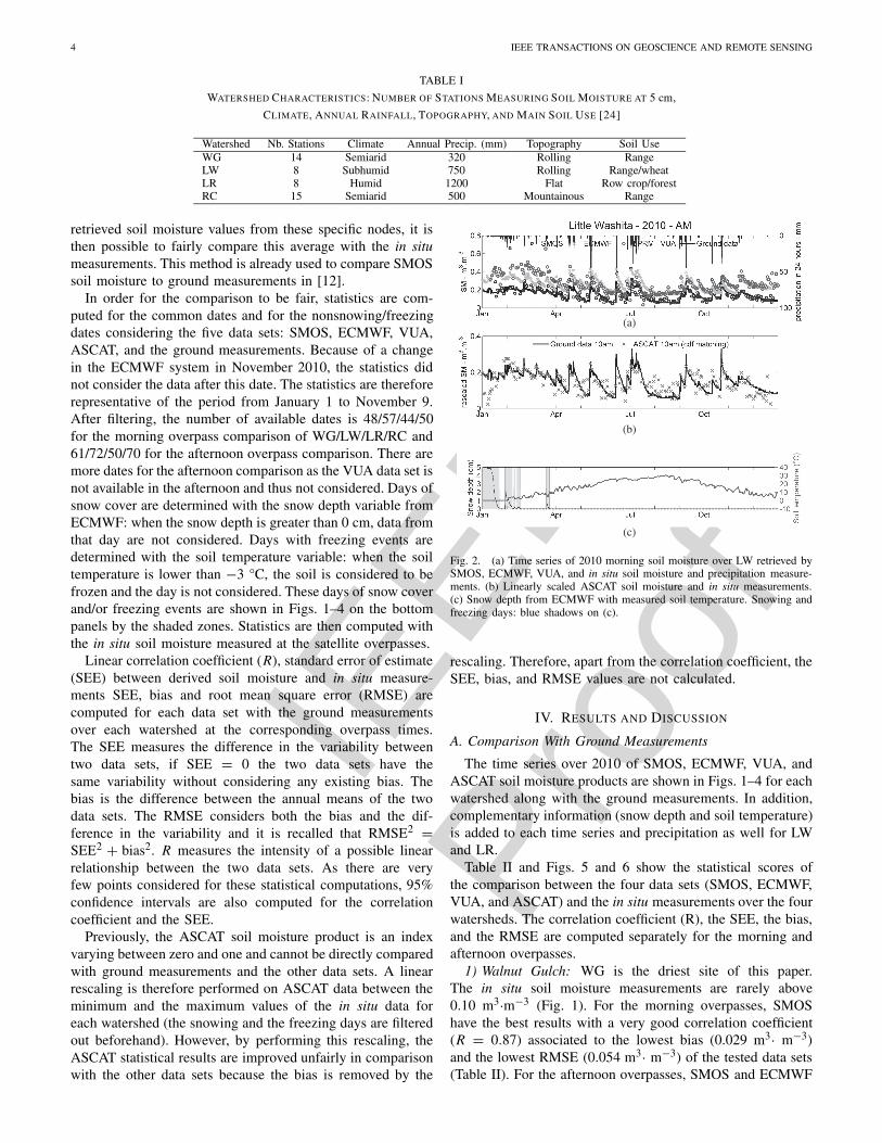
Fig. 1. (a) Time series of 2010 morning soil moisture over WG retrieved bySMOS, ECMWF, VUA, and in situ measurements. (b) Linearly scaled ASCATsoil moisture and in situ measurements. (c) Snow depth from ECMWF withmeasured soil temperature. Snowing and freezing days: blue shadows on (c).
checked during a field experiment and sensors/locations thatdid not agree well with the in situ observations are removed;3) a temporal stability analysis is performed with all the in situdata and bad locations are removed; and 4) the sensors thatdid not respond well (visually) to precipitation events areremoved. Soil moisture data are acquired every 30 min (hourlyfor RC). LW and LR watersheds are equipped with precipita-tion sensors that recorded data every 30 min. Table I showsthe characteristics of each watershed.
D. Snow Cover and Soil Temperature Information
Additional information on the snow presence over eachwatershed is used in this paper. The ECMWF snow covervariable is used to remove data during days of snow coverand freezing events. Like the ECMWF soil moisture product,the snow depth is available at SMOS resolution and overpasstime. It is natively available on a 0.225° grid every 3 hand is interpolated spatially and temporally to match SMOSrequirements for use in the SMOS algorithm. The snow depthrepresents the amount of snow in centimeter present at thesurface of the ground.
The soil temperature is also measured by the ground sta-tions. Like the soil moisture, the temperature values from thedifferent stations are given averaged over each watershed.
III. DATA PREPROCESSING AND METHODOLOGY
VUA and ASCAT grid products are first linearly interpo-lated on the SMOS grid. The distributed in situ soil moisturemeasurements are an average of different sensors representingan area that is comparable with a satellite footprint [24]. Thenetworks of the four watersheds are specially designed for thispurpose and the in situ data are furnished with a list of SMOSnodes that are covered by these networks. By averaging the
IEEE
Proo
f
4 IEEE TRANSACTIONS ON GEOSCIENCE AND REMOTE SENSING
TABLE I
WATERSHED CHARACTERISTICS: NUMBER OF STATIONS MEASURING SOIL MOISTURE AT 5 cm,
CLIMATE, ANNUAL RAINFALL, TOPOGRAPHY, AND MAIN SOIL USE [24]
Watershed Nb. Stations Climate Annual Precip. (mm) Topography Soil UseWG 14 Semiarid 320 Rolling RangeLW 8 Subhumid 750 Rolling Range/wheatLR 8 Humid 1200 Flat Row crop/forestRC 15 Semiarid 500 Mountainous Range
retrieved soil moisture values from these specific nodes, it isthen possible to fairly compare this average with the in situmeasurements. This method is already used to compare SMOSsoil moisture to ground measurements in [12].
In order for the comparison to be fair, statistics are com-puted for the common dates and for the nonsnowing/freezingdates considering the five data sets: SMOS, ECMWF, VUA,ASCAT, and the ground measurements. Because of a changein the ECMWF system in November 2010, the statistics didnot consider the data after this date. The statistics are thereforerepresentative of the period from January 1 to November 9.After filtering, the number of available dates is 48/57/44/50for the morning overpass comparison of WG/LW/LR/RC and61/72/50/70 for the afternoon overpass comparison. There aremore dates for the afternoon comparison as the VUA data set isnot available in the afternoon and thus not considered. Days ofsnow cover are determined with the snow depth variable fromECMWF: when the snow depth is greater than 0 cm, data fromthat day are not considered. Days with freezing events aredetermined with the soil temperature variable: when the soiltemperature is lower than −3 °C, the soil is considered to befrozen and the day is not considered. These days of snow coverand/or freezing events are shown in Figs. 1–4 on the bottompanels by the shaded zones. Statistics are then computed withthe in situ soil moisture measured at the satellite overpasses.
Linear correlation coefficient (R), standard error of estimate(SEE) between derived soil moisture and in situ measure-ments SEE, bias and root mean square error (RMSE) arecomputed for each data set with the ground measurementsover each watershed at the corresponding overpass times.The SEE measures the difference in the variability betweentwo data sets, if SEE = 0 the two data sets have thesame variability without considering any existing bias. Thebias is the difference between the annual means of the twodata sets. The RMSE considers both the bias and the dif-ference in the variability and it is recalled that RMSE2 =SEE2 + bias2. R measures the intensity of a possible linearrelationship between the two data sets. As there are veryfew points considered for these statistical computations, 95%confidence intervals are also computed for the correlationcoefficient and the SEE.
Previously, the ASCAT soil moisture product is an indexvarying between zero and one and cannot be directly comparedwith ground measurements and the other data sets. A linearrescaling is therefore performed on ASCAT data between theminimum and the maximum values of the in situ data foreach watershed (the snowing and the freezing days are filteredout beforehand). However, by performing this rescaling, theASCAT statistical results are improved unfairly in comparisonwith the other data sets because the bias is removed by the
(a)
(b)
(c)
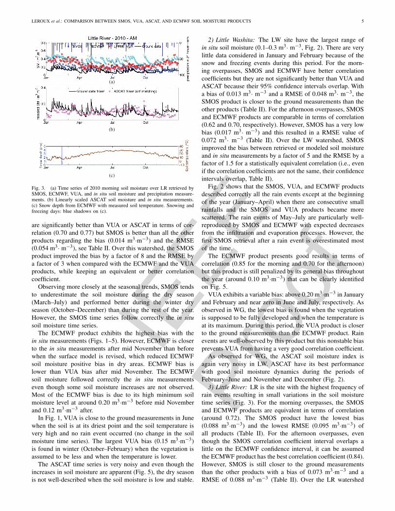
Fig. 2. (a) Time series of 2010 morning soil moisture over LW retrieved bySMOS, ECMWF, VUA, and in situ soil moisture and precipitation measure-ments. (b) Linearly scaled ASCAT soil moisture and in situ measurements.(c) Snow depth from ECMWF with measured soil temperature. Snowing andfreezing days: blue shadows on (c).
rescaling. Therefore, apart from the correlation coefficient, theSEE, bias, and RMSE values are not calculated.
IV. RESULTS AND DISCUSSION
A. Comparison With Ground Measurements
The time series over 2010 of SMOS, ECMWF, VUA, andASCAT soil moisture products are shown in Figs. 1–4 for eachwatershed along with the ground measurements. In addition,complementary information (snow depth and soil temperature)is added to each time series and precipitation as well for LWand LR.
Table II and Figs. 5 and 6 show the statistical scores ofthe comparison between the four data sets (SMOS, ECMWF,VUA, and ASCAT) and the in situ measurements over the fourwatersheds. The correlation coefficient (R), the SEE, the bias,and the RMSE are computed separately for the morning andafternoon overpasses.
1) Walnut Gulch: WG is the driest site of this paper.The in situ soil moisture measurements are rarely above0.10 m3·m−3 (Fig. 1). For the morning overpasses, SMOShave the best results with a very good correlation coefficient(R = 0.87) associated to the lowest bias (0.029 m3· m−3)and the lowest RMSE (0.054 m3· m−3) of the tested data sets(Table II). For the afternoon overpasses, SMOS and ECMWF
IEEE
Proo
f
LEROUX et al.: COMPARISON BETWEEN SMOS, VUA, ASCAT, AND ECMWF SOIL MOISTURE PRODUCTS 5
(a)
(b)
(c)
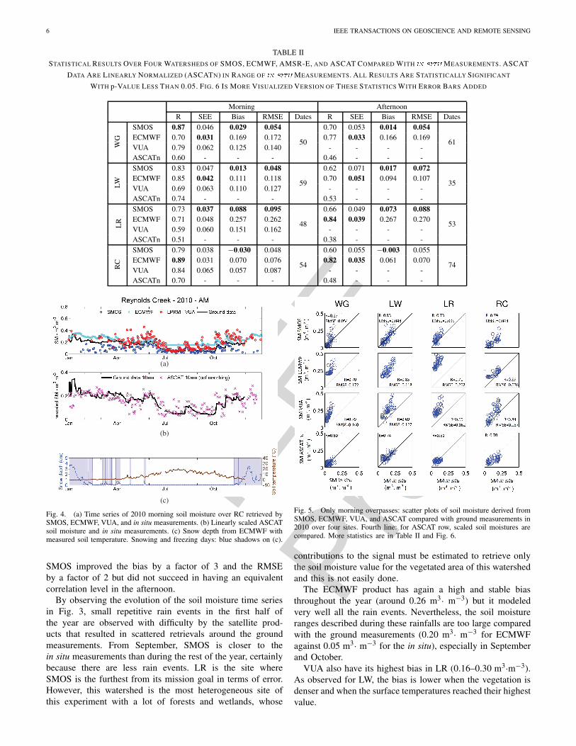
Fig. 3. (a) Time series of 2010 morning soil moisture over LR retrieved bySMOS, ECMWF, VUA, and in situ soil moisture and precipitation measure-ments. (b) Linearly scaled ASCAT soil moisture and in situ measurements.(c) Snow depth from ECMWF with measured soil temperature. Snowing andfreezing days: blue shadows on (c).
are significantly better than VUA or ASCAT in terms of cor-relation (0.70 and 0.77) but SMOS is better than all the otherproducts regarding the bias (0.014 m3·m−3) and the RMSE(0.054 m3· m−3), see Table II. Over this watershed, the SMOSproduct improved the bias by a factor of 8 and the RMSE bya factor of 3 when compared with the ECMWF and the VUAproducts, while keeping an equivalent or better correlationcoefficient.
Observing more closely at the seasonal trends, SMOS tendsto underestimate the soil moisture during the dry season(March–July) and performed better during the winter dryseason (October–December) than during the rest of the year.However, the SMOS time series follow correctly the in situsoil moisture time series.
The ECMWF product exhibits the highest bias with thein situ measurements (Figs. 1–5). However, ECMWF is closerto the in situ measurements after mid November than beforewhen the surface model is revised, which reduced ECMWFsoil moisture positive bias in dry areas. ECMWF bias islower than VUA bias after mid November. The ECMWFsoil moisture followed correctly the in situ measurementseven though some soil moisture increases are not observed.Most of the ECMWF bias is due to its high minimum soilmoisture level at around 0.20 m3·m−3 before mid Novemberand 0.12 m3·m−3 after.
In Fig. 1, VUA is close to the ground measurements in Junewhen the soil is at its driest point and the soil temperature isvery high and no rain event occurred (no change in the soilmoisture time series). The largest VUA bias (0.15 m3·m−3)is found in winter (October–February) when the vegetation isassumed to be less and when the temperature is lower.
The ASCAT time series is very noisy and even though theincreases in soil moisture are apparent (Fig. 5), the dry seasonis not well-described when the soil moisture is low and stable.
2) Little Washita: The LW site have the largest range ofin situ soil moisture (0.1–0.3 m3· m−3, Fig. 2). There are verylittle data considered in January and February because of thesnow and freezing events during this period. For the morn-ing overpasses, SMOS and ECMWF have better correlationcoefficients but they are not significantly better than VUA andASCAT because their 95% confidence intervals overlap. Witha bias of 0.013 m3· m−3 and a RMSE of 0.048 m3· m−3, theSMOS product is closer to the ground measurements than theother products (Table II). For the afternoon overpasses, SMOSand ECMWF products are comparable in terms of correlation(0.62 and 0.70, respectively). However, SMOS has a very lowbias (0.017 m3· m−3) and this resulted in a RMSE value of0.072 m3· m−3 (Table II). Over the LW watershed, SMOSimproved the bias between retrieved or modeled soil moistureand in situ measurements by a factor of 5 and the RMSE by afactor of 1.5 for a statistically equivalent correlation (i.e., evenif the correlation coefficients are not the same, their confidenceintervals overlap, Table II).
Fig. 2 shows that the SMOS, VUA, and ECMWF productsdescribed correctly all the rain events except at the beginningof the year (January–April) when there are consecutive smallrainfalls and the SMOS and VUA products became morescattered. The rain events of May–July are particularly well-reproduced by SMOS and ECMWF with expected decreasesfrom the infiltration and evaporation processes. However, thefirst SMOS retrieval after a rain event is overestimated mostof the time.
The ECMWF product presents good results in terms ofcorrelation (0.85 for the morning and 0.70 for the afternoon)but this product is still penalized by its general bias throughoutthe year (around 0.10 m3·m−3) that can be clearly identifiedon Fig. 5.
VUA exhibits a variable bias: above 0.20 m3·m−3 in Januaryand February and near zero in June and July, respectively. Asobserved in WG, the lowest bias is found when the vegetationis supposed to be fully developed and when the temperature isat its maximum. During this period, the VUA product is closerto the ground measurements than the ECMWF product. Rainevents are well-observed by this product but this nonstable biasprevents VUA from having a very good correlation coefficient.
As observed for WG, the ASCAT soil moisture index isagain very noisy in LW. ASCAT have its best performancewith good soil moisture dynamics during the periods ofFebruary–June and November and December (Fig. 2).
3) Little River: LR is the site with the highest frequency ofrain events resulting in small variations in the soil moisturetime series (Fig. 3). For the morning overpasses, the SMOSand ECMWF products are equivalent in terms of correlation(around 0.72). The SMOS product have the lowest bias(0.088 m3·m−3) and the lowest RMSE (0.095 m3·m−3) ofall products (Table II). For the afternoon overpasses, eventhough the SMOS correlation coefficient interval overlaps alittle on the ECMWF confidence interval, it can be assumedthe ECMWF product has the best correlation coefficient (0.84).However, SMOS is still closer to the ground measurementsthan the other products with a bias of 0.073 m3·m−3 and aRMSE of 0.088 m3·m−3 (Table II). Over the LR watershed
IEEE
Proo
f
6 IEEE TRANSACTIONS ON GEOSCIENCE AND REMOTE SENSING
TABLE II
STATISTICAL RESULTS OVER FOUR WATERSHEDS OF SMOS, ECMWF, AMSR-E, AND ASCAT COMPARED WITH �� ���� MEASUREMENTS. ASCAT
DATA ARE LINEARLY NORMALIZED (ASCATN) IN RANGE OF �� ���� MEASUREMENTS. ALL RESULTS ARE STATISTICALLY SIGNIFICANT
WITH p-VALUE LESS THAN 0.05. FIG. 6 IS MORE VISUALIZED VERSION OF THESE STATISTICS WITH ERROR BARS ADDED
Morning AfternoonR SEE Bias RMSE Dates R SEE Bias RMSE Dates
SMOS 0.87 0.046 0.029 0.054
50
0.70 0.053 0.014 0.054ECMWF 0.70 0.031 0.169 0.172 0.77 0.033 0.166 0.169VUA 0.79 0.062 0.125 0.140 - - - -W
G
ASCATn 0.60 - - - 0.46 - - -
61
SMOS 0.83 0.047 0.013 0.048 0.62 0.071 0.017 0.072
35ECMWF 0.85 0.042 0.111 0.118 0.70 0.051 0.094 0.107VUA 0.69 0.063 0.110 0.127 - - - -LW
ASCATn 0.74 - - -
59
0.53 - - -
SMOS 0.73 0.037 0.088 0.095
48
0.66 0.049 0.073 0.088ECMWF 0.71 0.048 0.257 0.262 0.84 0.039 0.267 0.270VUA 0.59 0.060 0.151 0.162 - - - -L
R
ASCATn 0.51 - - - 0.38 - - -
53
SMOS 0.79 0.038 −0.030 0.048 0.60 0.055 −0.003 0.055
74ECMWF 0.89 0.031 0.070 0.076 0.82 0.035 0.061 0.070VUA 0.84 0.065 0.057 0.087 - - - -R
C
ASCATn 0.70 - - -
54
0.48 - - -
(a)
(b)
(c)
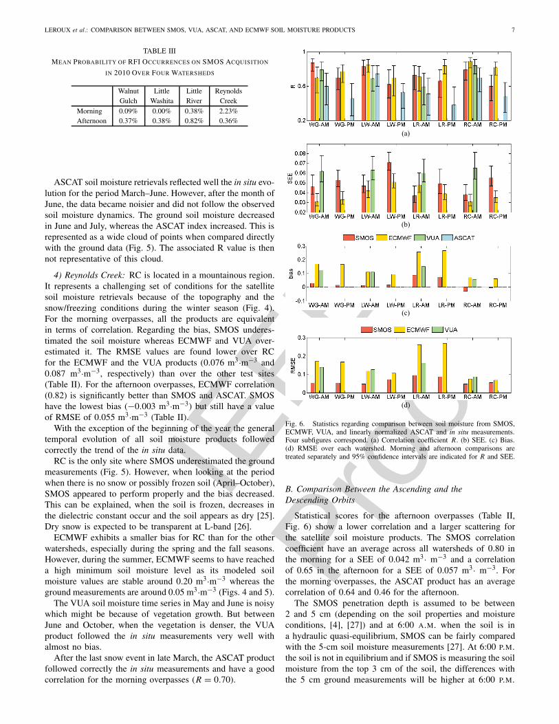
Fig. 4. (a) Time series of 2010 morning soil moisture over RC retrieved bySMOS, ECMWF, VUA, and in situ measurements. (b) Linearly scaled ASCATsoil moisture and in situ measurements. (c) Snow depth from ECMWF withmeasured soil temperature. Snowing and freezing days: blue shadows on (c).
SMOS improved the bias by a factor of 3 and the RMSEby a factor of 2 but did not succeed in having an equivalentcorrelation level in the afternoon.
By observing the evolution of the soil moisture time seriesin Fig. 3, small repetitive rain events in the first half ofthe year are observed with difficulty by the satellite prod-ucts that resulted in scattered retrievals around the groundmeasurements. From September, SMOS is closer to thein situ measurements than during the rest of the year, certainlybecause there are less rain events. LR is the site whereSMOS is the furthest from its mission goal in terms of error.However, this watershed is the most heterogeneous site ofthis experiment with a lot of forests and wetlands, whose
Fig. 5. Only morning overpasses: scatter plots of soil moisture derived fromSMOS, ECMWF, VUA, and ASCAT compared with ground measurements in2010 over four sites. Fourth line: for ASCAT row, scaled soil moistures arecompared. More statistics are in Table II and Fig. 6.
contributions to the signal must be estimated to retrieve onlythe soil moisture value for the vegetated area of this watershedand this is not easily done.
The ECMWF product has again a high and stable biasthroughout the year (around 0.26 m3· m−3) but it modeledvery well all the rain events. Nevertheless, the soil moistureranges described during these rainfalls are too large comparedwith the ground measurements (0.20 m3· m−3 for ECMWFagainst 0.05 m3· m−3 for the in situ), especially in Septemberand October.
VUA also have its highest bias in LR (0.16–0.30 m3·m−3).As observed for LW, the bias is lower when the vegetation isdenser and when the surface temperatures reached their highestvalue.
IEEE
Proo
f
LEROUX et al.: COMPARISON BETWEEN SMOS, VUA, ASCAT, AND ECMWF SOIL MOISTURE PRODUCTS 7
TABLE III
MEAN PROBABILITY OF RFI OCCURRENCES ON SMOS ACQUISITION
IN 2010 OVER FOUR WATERSHEDS
Walnut Little Little ReynoldsGulch Washita River Creek
Morning 0.09% 0.00% 0.38% 2.23%Afternoon 0.37% 0.38% 0.82% 0.36%
ASCAT soil moisture retrievals reflected well the in situ evo-lution for the period March–June. However, after the month ofJune, the data became noisier and did not follow the observedsoil moisture dynamics. The ground soil moisture decreasedin June and July, whereas the ASCAT index increased. This isrepresented as a wide cloud of points when compared directlywith the ground data (Fig. 5). The associated R value is thennot representative of this cloud.
4) Reynolds Creek: RC is located in a mountainous region.It represents a challenging set of conditions for the satellitesoil moisture retrievals because of the topography and thesnow/freezing conditions during the winter season (Fig. 4).For the morning overpasses, all the products are equivalentin terms of correlation. Regarding the bias, SMOS underes-timated the soil moisture whereas ECMWF and VUA over-estimated it. The RMSE values are found lower over RCfor the ECMWF and the VUA products (0.076 m3·m−3 and0.087 m3·m−3, respectively) than over the other test sites(Table II). For the afternoon overpasses, ECMWF correlation(0.82) is significantly better than SMOS and ASCAT. SMOShave the lowest bias (−0.003 m3·m−3) but still have a valueof RMSE of 0.055 m3·m−3 (Table II).
With the exception of the beginning of the year the generaltemporal evolution of all soil moisture products followedcorrectly the trend of the in situ data.
RC is the only site where SMOS underestimated the groundmeasurements (Fig. 5). However, when looking at the periodwhen there is no snow or possibly frozen soil (April–October),SMOS appeared to perform properly and the bias decreased.This can be explained, when the soil is frozen, decreases inthe dielectric constant occur and the soil appears as dry [25].Dry snow is expected to be transparent at L-band [26].
ECMWF exhibits a smaller bias for RC than for the otherwatersheds, especially during the spring and the fall seasons.However, during the summer, ECMWF seems to have reacheda high minimum soil moisture level as its modeled soilmoisture values are stable around 0.20 m3·m−3 whereas theground measurements are around 0.05 m3·m−3 (Figs. 4 and 5).
The VUA soil moisture time series in May and June is noisywhich might be because of vegetation growth. But betweenJune and October, when the vegetation is denser, the VUAproduct followed the in situ measurements very well withalmost no bias.
After the last snow event in late March, the ASCAT productfollowed correctly the in situ measurements and have a goodcorrelation for the morning overpasses (R = 0.70).
(a)
(b)
(c)
(d)
Fig. 6. Statistics regarding comparison between soil moisture from SMOS,ECMWF, VUA, and linearly normalized ASCAT and in situ measurements.Four subfigures correspond. (a) Correlation coefficient R. (b) SEE. (c) Bias.(d) RMSE over each watershed. Morning and afternoon comparisons aretreated separately and 95% confidence intervals are indicated for R and SEE.
B. Comparison Between the Ascending and theDescending Orbits
Statistical scores for the afternoon overpasses (Table II,Fig. 6) show a lower correlation and a larger scattering forthe satellite soil moisture products. The SMOS correlationcoefficient have an average across all watersheds of 0.80 inthe morning for a SEE of 0.042 m3· m−3 and a correlationof 0.65 in the afternoon for a SEE of 0.057 m3· m−3. Forthe morning overpasses, the ASCAT product has an averagecorrelation of 0.64 and 0.46 for the afternoon.
The SMOS penetration depth is assumed to be between2 and 5 cm (depending on the soil properties and moistureconditions, [4], [27]) and at 6:00 A.M. when the soil is ina hydraulic quasi-equilibrium, SMOS can be fairly comparedwith the 5-cm soil moisture measurements [27]. At 6:00 P.M.the soil is not in equilibrium and if SMOS is measuring the soilmoisture from the top 3 cm of the soil, the differences withthe 5 cm ground measurements will be higher at 6:00 P.M.
IEEE
Proo
f
8 IEEE TRANSACTIONS ON GEOSCIENCE AND REMOTE SENSING
than at 6:00 A.M. [27] recommended using morning mea-surements when comparing with space observations becauseof the day-time decoupling that could occur in the afternoonbecause of the nonhydraulic equilibrium of the soil. The sameexplanations apply for the ASCAT results at 9:30 A.M. and at9:30 P.M. These results are consistent with the results of [28].
Another possible explanation for these differences betweenthe morning and the afternoon results is still related to thenonequilibrium of the soil and it concerns the assumptions aremade concerning the soil surface temperature. It is assumedthat the soil and the vegetation temperatures are approximatelyequal, which is a fair assumption during the night or earlymorning but during the day, the vegetation temperature isexpected to be closer to the air temperature than to thesoil temperature. This assumption of equal vegetation andeffective soil temperatures can lead to less accurate satellitesoil moisture retrievals in the afternoon.
Regarding SMOS results, one last possibility could be thepresence of RFIs that are only seen during the descendingorbits when the satellite is going in the afternoon fromnorth to south and is pointing in the southwest direc-tion. From the RFI contamination probability maps derivedfrom the mixed polarized acquisitions (real and imaginaryparts [16], [29]), it is possible to compute for each watershedthe mean probability of RFI occurrences (Table III). Exceptover RC, the probability of RFI contamination is higher for theafternoon overpasses even if they are still very low comparedwith highly contaminated regions such as Asia. This differencein RFI contamination between the morning and the afternoonoverpasses might partially explain why SMOS results arebetter in the morning.
V. CONCLUSION
SMOS data were compared with in situ observations andother satellite data and model outputs. SMOS, VUA, ECMWF,and ASCAT soil moisture retrievals were compared with thein situ measurements and intercompared over four differentsites in the U.S. under various climate conditions and soilcharacteristics.
Over the four test sites, no specific product had a sig-nificantly better correlation with the ground measurements.Since this paper only covers the year 2010, 35–74 commondates were considered to compute the statistics and resultedin substantial confidence intervals that made all productsequivalent in terms of correlation. The statistical parametersused to differentiate the four data sets were the SEE, thebias, and logically the RMSE. Over most of the watersheds,ECMWF had a significantly lower SEE (0.039 m3· m−3 inaverage) than SMOS (0.049 m3· m−3 in average) and VUA(0.063 m3· m−3 for the morning only), representing a lessscattered data set. ECMWF soil moisture time evolution wasvery close to the ground measurements with clear identifica-tions of the rainfall events and the soil drainage afterward.However, SMOS had clearly the lowest bias with an averageof 0.032 m3· m−3 whereas ECMWF had a mean bias of0.150 m3· m−3 and VUA of 0.129 m3· m−3. SMOS also hadthe lowest RMSE over all the sites except RC. SMOS had
a mean RMSE of 0.064 m3· m−3 whereas ECMWF had amean RMSE of 0.156 m3· m−3 and VUA of 0.129 m3· m−3
(for the morning only). Therefore, although the SMOS missionaccuracy objective of 0.040 m3· m−3 was not reached overthese four watersheds in 2010, SMOS improved the totalRMSE by a factor of at least 2 on average in 2010 for anequivalent correlation compared with the other soil moistureproducts.
The time series analysis revealed a positive constant biasin the ECMWF data set: 0.17/0.10/ 0.26/0.07 m3· m−3,respectively for the WG/LW/LR/RC watersheds. Even aftermid-November when the surface model and analysis wererevised, this bias was still present over all the watersheds buthad decreased over WG (data after mid-November were notconsidered in the statistical results). Despite very good corre-lation coefficients, this minimum level was a major obstacle inusing ECMWF for the four test sites. VUA also had a bias butwas not constant and appeared to evolve with the seasons. Thebias was higher when the vegetation and the soil temperaturewere low (during winter) and tended to decrease when thevegetation was supposed to be denser and the soil temperatureincreasing to its maximum in the summer, resulting in a quasi-null bias. This evolution of the VUA bias throughout the yearwas assumed to be linked to a physical parameter such as thevegetation or the temperature since it evolved with the seasonsand because the AMSR-E frequencies (6.9 and 10.7 GHz)were more sensitive to the vegetation layer than SMOS at1.4 GHz. It was also possible that this bias was due to the soileffective temperature that was modeled through the 36-GHzbrightness temperature or to another assumption that was madein the VUA algorithm. The ASCAT soil moisture index wasvery noisy in comparison with the other products and eventhough some rain events were obvious in the retrievals, thein situ soil moisture dynamics were not well-represented forany of the watersheds. Active microwave observations werevery sensitive to surface roughness and WG, for example,had sandy soils with significant amount of gravel. These soilcharacteristics resulted in a greater surface roughness whichcould explain partially the poor results of ASCAT.
The comparison of the statistical performances of theproducts between the morning and the afternoon revealedthat the ECMWF model did not show significant differenceswhereas the satellite SMOS and ASCAT products showedseveral differences: R = 0.80/0.65, SE E = 0.042/0.057 m3·m−3, bias = 0.040/0.027 m3· m−3, RMSE =0.061/0.067 m3· m−3 for SMOS, and R = 0.64/0.46 forASCAT (A.M./P.M. in average over the four watersheds).These differences in performance can be explained that inthe morning, the soil was in hydraulic quasi-equilibrium. Onthe other hand for the afternoon, this comparison might notbe as correct as for the morning. Another explanation couldbe the inaccurate modeling of the soil and the vegetationtemperatures in the retrieval algorithm. They were assumedto be equal and this assumption might not be true in theafternoon when the vegetation temperature was expected tobe closer to the air temperature than to the soil temperature.The last possible explanation for SMOS performancedifference concerned the RFI. The occurrence probabilities of
IEEE
Proo
f
LEROUX et al.: COMPARISON BETWEEN SMOS, VUA, ASCAT, AND ECMWF SOIL MOISTURE PRODUCTS 9
RFI in 2010 were higher in the afternoon than in the morningexcept over RC.
The results of this paper concur with the different studiesthat were realized in the frame of the SMOS soil moistureproduct validation [11], [12], [14], [30]. SMOS soil moistureretrievals were already very close to the ground measurementsbut need to be improved to meet its scientific goal of an errorless than 0.04 m3· m−3. In this perspective, a new versionof the level 2 soil moisture processor (v5.51) was already inplace since March 2012 and allowed to switch between theDobson and the Mironov constant dielectric model and thisversion showed promising first results.
The main advantage in comparing satellite products wasthe possibility of comparing with global coverage and furtherstudies will be developed in this direction in the near future.
ACKNOWLEDGMENT
The authors would like to thank the U.S. Department ofAgriculture (Agricultural Research Service) for providing theground data.
REFERENCES
[1] “Implementation plan for the global observing system for climate insupport of the UNFCCC,” World Meteorological Organ., Intergovern.Oceanogr. Commission, United Nations Environ. Progr., InternationalCouncil Science, Geneva, Switzerland, Tech. Rep. 1244, 2010.
[2] M. Drusch, “Initializing numerical weather predictions models withsatellite derived surface soil moisture: Data assimilation experimentswith ECMWF’s integrated forecast system and the TMI soil moisturedata set,” J. Geophys. Res., vol. 113, no. D3, p. D03102, Feb. 2007.
[3] H. Douville and F. Chauvin, “Relevance of soil moisture for seasonalclimate predictions: A preliminary study,” Climate Dynamics, vol. 16,nos. 10–11, pp. 719–736, Oct. 2000.
[4] Y. Kerr, P. Waldteufel, J. Wigneron, S. Delwart, F. Cabot, J. Boutin,M. Escorihuela, J. Font, N. Reul, C. Gruhier, S. Juglea, M. Drinkwater,A. Hahne, M. Martin-Neira, and S. Mecklenburg, “The SMOS mission:New tool for monitoring key elements of the global water cycle,” Proc.IEEE, vol. 98, no. 5, pp. 666–687, May 2010.
[5] D. Entekhabi, E. Njoku, P. E. O. Neill, K. Kellogg, W. Crow, W. Edel-stein, J. Entin, S. Goodman, T. Jackson, J. Johnson, J. Kimball, J. Piep-meier, R. Koster, N. Martin, K. McDonald, M. Moghaddam, S. Moran,R. Reichle, J. Shi, M. Spencer, S. Thurman, L. Tsang, and J. Zyl, “Thesoil moisture active passive (smap) mission,” Proc. IEEE, vol. 98, no. 5,pp. 704–716, May 2010.
[6] Y. Kerr, P. Waldteufel, J. Wigneron, J. Martinuzzi, J. Font, andM. Berger, “Soil moisture retrieval from space: The soil moisture andocean salinity (SMOS) mission,” IEEE Trans. Geosci. Remote Sens.,vol. 39, no. 8, pp. 1729–1735, Aug. 2001.
[7] M. Owe, R. de Jeu, and J. Walker, “A methodology for surface soilmoisture and vegetation optical depth retrieval using the microwavepolarization difference index,” IEEE Trans. Geosci. Remote Sens.,vol. 39, no. 8, pp. 1643–1654, Aug. 2001.
[8] E. Njoku, T. Jackson, V. Lakshmi, T. Chan, and S. Nghiem, “Soilmoisture retrieval from ASMR-E,” IEEE Trans. Geosci. Remote Sens.,vol. 41, no. 2, pp. 215–229, Feb. 2003.
[9] L. Li, P. Gaiser, B. Gao, R. Bevilacqua, T. Jackson, E. Njoku, C. Rüdiger,J. Calvet, and R. Bindlish, “Windsat global soil moisture retrievaland validation,” IEEE Trans. Geosci. Remote Sens., vol. 48, no. 5,pp. 2224–2241, May 2010.
[10] V. Naeimi, K. Scipal, Z. Bartalis, and S. H. W. Wagner, “An improvedsoil moisture retrieval algorithm for ERS and METOP scatterometerobservations,” IEEE Trans. Geosci. Remote Sens., vol. 47, no. 7,pp. 1999–2013, Jul. 2009.
[11] A. A. Bitar, D. Leroux, Y. Kerr, O. Merlin, P. Richaume, A. Sahoo, andE. Wood, “Evaluation of SMOS soil moisture products over continentalU.S. Using SCAN/SNOTEL network,” IEEE Trans. Geosci. RemoteSens., vol. 50, no. 5, pp. 1572–1586, May 2012.
[12] T. Jackson, R. Bindlish, M. Cosh, T. Zhao, P. Starks, D. Bosch,M. Seyfried, S. Moran, Y. Kerr, and D. Leroux, “Validation of soilmoisture ocean salinity (SMOS) soil moisture over watershed networksin the U.S.,” IEEE Trans. Geosci. Remote Sens., vol. 50, no. 5,pp. 1530–1543, May 2012.
[13] J. Wigneron, Y. Kerr, P. Waldteufel, K. Saleh, M. Escorihuela,P. Richaume, P. Ferrazzoli, P. de Rosnay, R. Gurney, J. Calvet,J. Grant, M. Guglielmetti, B. Hornbuckle, C. Mätzler, T. Pellarin, andM. Schwank, “L-band microwave emission of the biosphere (L-MEB)model: Description and calibration against experimental data sets overcrop fields,” Remote Sens. Environ., vol. 107, no. 4, pp. 639–655,Apr. 2007.
[14] Y. Kerr, P. Waldteufel, P. Richaume, J. Wigneron, P. Ferrazzoli, A. Mah-moodi, A. Al Bitar, F. Cabot, C. Gruhier, S. Juglea, D. Leroux,A. Mialon, and S. Delwart, “The SMOS soil moisture retrieval algo-rithm,” IEEE Trans. Geosci. Remote Sens., vol. 50, no. 5, pp. 1384–1403,May 2012.
[15] V. Masson, J.-L. Champeau, F. Chauvin, C. Meriguet, and R. Lacaze,“A global data base of land surface parameters at 1-km resolutionin meteorological and climate models,” J. Climate, vol. 16, no. 9,pp. 1261–1282, May 2003.
[16] “Algorithm theoretical basis document,” Tech. Rep. 3.d, CESBIO,Toulouse, France, IPSL, Paris, France, INRA-EPHYSE, Bordeaux,France, Reading University, Reading, England, Tor Vergata University,Rome, Italy, 2010.
[17] D. Carr, R. Kahn, K. Sahr, and T. Olsen, “Isea discrete global grids,”Stat. Comput. Stat. Graph. Newlett., vol. 8, nos. 2–3, pp. 31–39, 1997.
[18] W. Wagner, G. Lemoine, and H. Rott, “A method for estimating soilmoisture from ERS scatterometer and soil data,” Remote Sens. Environ.,vol. 70, no. 2, pp. 191–207, Nov. 1999.
[19] “AMSR-E data users handbook,” Japan Aerospace Exploration Agency(JAXA), Washington, DC, USA, Tech. Rep. NCX-030021, Mar. 2006.
[20] C. Gruhier, P. de Rosnay, Y. Kerr, E. Mougin, E. Ceschia, J. Calvet, andP. Richaume, “Evaluation of AMSR-E soil moisture product based onground measurements over temperate and semi-arid regions,” Geophys.Res. Lett., vol. 35, no. 10, p. L10405, May 2008.
[21] C. Rudiger, J. C. Calvet, C. Gruhier, T. Holmes, R. de Jeu, and W. Wag-ner, “An intercomparison of ERS-Scat and AMSR-E soil moistureobservations with model simulations over france,” Amer. Meteorol. Soc.,vol. 10, no. 2, pp. 431–447, Apr. 2009.
[22] C. Draper, J. Walker, P. Steinle, R. de Jeu, and T. Holmes, “An evalu-ation of AMSR-E derived soil moisture over Australia,” Remote Sens.Environ., vol. 113, no. 4, pp. 703–710, Apr. 2009.
[23] C. Gruhier, P. de Rosnay, S. Hasenauer, T. Holmes, R. de Jeu, Y. Kerr,E. Mougin, E. Njoku, F. Timouk, W. Wagner, and M. Zribi, “Soilmoisture active and passive microwave products: Intercomparison andevaluation over a sahelian site,” Hydrol. Earth Syst. Sci., vol. 14, no. 1,pp. 141–156, Jan. 2010.
[24] T. Jackson, M. Cosh, R. Bindlish, P. Starks, D. Bosch, M. Seyfried,D. Goodrich, M. Moran, and J. Du, “Validation of advancedmicrowave scanning radiometer soil moisture products,” IEEETrans. Geosci. Remote Sens., vol. 48, no. 12, pp. 4256–4272,Dec. 2010.
[25] C. Matzler, “Passive microwave signatures of landscapes in winter,”Meteorol. Atmospheric Phys., vol. 54, nos. 1–4, pp. 241–260, 1994.
[26] R. Armstrong and M. Brodzik, “A twenty year record of global snowcover fluctuations derived from passive microwave remote sensing data,”in Proc. 5th Conf. Polar Meteorol. Oceanography, Amer. Meteorol. Soc.,Dallas, TX, USA, 1999, pp. 113–117.
[27] T. Jackson, “Profile soil moisture from space measurements,” J. Irrigat.Drainage Divis., ASCE, vol. 106, pp. 81–92, Mar. 1980.
[28] C. Albergel, C. Rüdiger, D. Carrer, J. Calvet, N. Fritz, V. Naeimi,Z. Bartalis, and S. Hasenauer, “An evaluation of ascat surfacesoil moisture products with in-situ observations in southwesternfrance,” Hydrol. Earth Syst. Sci., vol. 13, no. 2, pp. 115–124,2009.
[29] R. Oliva, E. Daganzo-Eusebio, Y. Kerr, S. Mecklenburg,S. Nieto, P. Richaume, and C. Gruhier, “SMOS radio frequencyinterference scenario: Status and actions taken to improve theRFI environment in the 1400–1427 MHz passive band,” IEEETrans. Geosci. Remote Sens., vol. 50, no. 5, pp. 1427–1439,May 2012.
[30] C. Albergel, P. de Rosnay, C. Gruhier, J. Munoz-Sabater, S. H. L. Isak-sen, Y. Kerr, and W. Wagner, “Evaluation of remotely sensedand modelled soil moisture products using global ground-based insitu observations,” Remote Sens. Environ., vol. 118, pp. 215–226,Mar. 2012.

IEEE
Proo
f
10 IEEE TRANSACTIONS ON GEOSCIENCE AND REMOTE SENSING
DELPHINE J. Leroux received the M.S. degreein applied mathematics from Institut National desSciences Appliquees, Toulouse, France, in 2009,and the Ph.D. degree in spatial hydrology fromUniversite Paul Sabatier, Toulouse, France, in 2012.
She was with the Centre d’Etudes Spatiales de laBiosphere, Toulouse, from 2009 to 2012, where sheworked on the validation of the soil moisture andocean salinity soil moisture product at the local andthe global scales by using statistical and physicalmethods. Currently, she is with the Jet Propulsion
Laboratory, Pasadena, CA, USA, where she works on the soil moisture activepassive mission.
Yann H. Kerr (M’88–SM’01–F’13) received theEngineering degree from Ecole Nationale Suprieurede l’Aronautique et de l’Espace, the M.Sc. degree inelectronics and electrical engineering from GlasgowUniversity, Glasgow, U.K., and the Ph.D. degree inAstrophysique Gophysique et Techniques Spatiales,Universit Paul Sabatier, Toulouse, France.
He is currently the Director of Centre dEtudesSpatiales de la BIOsphre, Toulouse, France. He wasan Earth Observation System Principal Investiga-tor (interdisciplinary investigations) and a Principal
Investigator and precursor of the use of the scatterometer over land. In 1990,he started to work on the interferometric concept applied to passive microwaveearth observation and was subsequently the science lead on the microwaveimaging radiometer with aperture synthesis project for the European SpaceAgency. In 1997, he proposed the SMOS Mission, the natural outcome of theprevious MIRAS work. He is currently involved in the exploitation of SMOSdata, in the calibration/validation activities and related level 2 soil moistureand level 3 and 4 developments. He is working on the SMOS next concept.His current research interests include theory and techniques for microwave andthermal infrared remote sensing of the Earth, with emphasis on hydrology,and water resources management.
Dr. Kerr was a recipient of the World Meteorological Organization 1stprize (Norbert Gerbier), the USDA Secretary’s Team Award for Excellence(Salsa Program), the Geoscience and Remote Sensing Society certificateof recognition for leadership in development of the first synthetic aperturemicrowave radiometer in space and success of the SMOS mission, and theDistinguished Lecturer for GRSS.
Ahmad Al Bitar received the M.E. degree in civilengineering from INSA-Lyon, Villeurbanne, France,in 2003, and the Ph.D. degree in hydrogeologyfrom Institut National Polytechnique de Toulouse,Toulouse, France, in 2006. His thesis work focuseson numerical modeling in stochastic porous media.
He joined CESBIO, Toulouse, France, in 2006. Hiscurrent research interests include integrated hydro-logical modeling and assimilation of remote sensingdata.
Rajat Bindlish (S’98–AM’99–M’03–SM’05)received the B.S. degree in civil engineeringfrom the Indian Institute of Technology, Bombay,India, in 1993, and the M.S. and Ph.D. degreesin civil engineering from The Pennsylvania StateUniversity, University Park, PA, USA, in 1996 and2000, respectively.
He is currently with the USDA AgriculturalResearch Service, Hydrology and Remote SensingLaboratory, Beltsville, MD, USA. He is currentlyworking on soil moisture estimation from microwave
sensors and their subsequent application in land surface hydrology. Hiscurrent research interests include the application of microwave remotesensing in hydrology.
Thomas J. Jackson (SM’96–F’02) received thePh.D. degree from the University of Maryland, Col-lege Park, MD, USA, in 1976.
He is a Research Hydrologist with the U.S. Depart-ment of Agriculture, Agricultural Research Service,Hydrology and Remote Sensing Laboratory. Hisresearch involves the application and developmentof remote sensing technology in hydrology andagriculture, primarily microwave measurement ofsoil moisture. He has been a member of the Sci-ence and Validation Teams of the Aqua, ADEOS-II
(Advanced Earth Observing Satellite), Radarsat, Oceansat-1, Envisat, ALOS(Advanced Land Observing Satellite), SMOS, Aquarius, GCOM-W (GlobalChange Observation Mission - Water), and SMAP remote sensing satellites.
Dr. Jackson is a Fellow of the Society of Photo-Optical InstrumentationEngineers, the American Meteorological Society, and the American Geophys-ical Union. In 2003, he was a recipient of the William T. Pecora Award(NASA and Department of Interior) for outstanding contributions towardunderstanding the Earth by means of remote sensing and the AmericanGeophysical Union Hydrologic Sciences Award for outstanding contributionsto the science of hydrology. He was a recipient of the IEEE Geoscience andRemote Sensing Society Distinguished Achievement Award in 2011.
Beatrice Berthelot received the Ph.D. degree inoceanography to estimate the ocean primary produc-tion using ocean color data in 1991.
She has considerable expertise in satellite remotesensing both over ocean and land. She was a Post-Doctoral with the California Space Institute, CA,USA, and Scripps Institution for Oceanography,USA. From 1993 to 2000, she was a ResearchEngineer with the Centre dEtude Spatiales de laBIOsphere, Toulouse, France. She developed dataprocessing chains for long time series of AVHRR
satellite dataset from 1983 to 1995, including calibration monitoring,atmospheric corrections, cloud and snow detection, and associated qualityflags. She developed the atmospheric correction algorithm scheme whichis applied at Centre de Traitement des Images VEGETATION. From 2000to 2006, she was the Terrestrial Biosphere Group Leader with NOVELTIS,Toulouse. She worked on multiple projects for CNES, ESA and EC, such asCYCLOPES FP5, from 2003 to 2006, the development of MERIS algorithmover land including atmosphere products and vegetation products ESA, from2004 to 2006, GLOBCOVER for the assessment and development of thecloud mask for MERIS. She worked on SMOS soil moisture simulations andretrieval using neural networks. She joined VEGA Technologies in 2008 asa Leader of Scientific Algorithms Group, when she worked on radiometriccalibration (test sites project, ESRIN), and managed the development of theapplication dedicated to the absolute radiometric calibration of HR satellites(ROSAS, 2011). She was involved in the development of the Level 2 Sentinel2 product and algorithm definition, for the atmospheric correction algorithmdevelopment and pixel classification definitions. Since October 2011, she hasbeen with MAGELLIUM in the data and signal processing department. Sheis the Project Manager for the development of vicarious calibration methodinside the DIMITRI ESA software. She has large expertise on radiativetransfer in the atmosphere.
Gautier Portet received an Associate degree insoftware development.
He is a Software Developer with Telespazio,France, and has been working on the Geoland2 SoilWater Index processing chain.
IEEE
Proo
f
IEEE TRANSACTIONS ON GEOSCIENCE AND REMOTE SENSING 1
Comparison Between SMOS, VUA, ASCAT, andECMWF Soil Moisture Products Over Four
Watersheds in U.S.DELPHINE J. Leroux, Yann H. Kerr, Fellow, IEEE, Ahmad Al Bitar, Rajat Bindlish, Senior Member, IEEE,
Thomas J. Jackson, Fellow, IEEE, Beatrice Berthelot, and Gautier Portet
Abstract— As part of the Soil Moisture and Ocean Salinity(SMOS) validation process, a comparison of the skills of threesatellites [SMOS, Advanced Microwave Scanning Radiometer-Earth Observing System (AMSR-E) or Advanced MicrowaveScanning Radiometer, and Advanced Scatterometer (ASCAT)],and one-model European Centre for Medium Range WeatherForecasting (ECMWF) soil moisture products is conducted overfour watersheds located in the U.S. The four products comparedin for 2010 over four soil moisture networks were used for thecalibration of AMSR-E. The results indicate that SMOS retrievalsare closest to the ground measurements with a low average rootmean square error of 0.061 m 3· m−3 for the morning overpassand 0.067 m 3· m−3 for the afternoon overpass, which representsan improvement by a factor of 2–3 compared with the otherproducts. The ECMWF product has good correlation coefficients(around 0.78) but has a constant bias of 0.1–0.2 m 3· m−3 overthe four networks. The land parameter retrieval model AMSR-Eproduct gives reasonable results in terms of correlation (around0.73) but has a variable seasonal bias over the year. The ASCATsoil moisture index is found to be very noisy and unstable.
Index Terms— Soil moisture, Soil Moisture and Ocean Salinity(SMOS), validation.
I. INTRODUCTION
SOIL moisture is an important variable in the study ofseasonal climate evolution and prediction as it plays a
major role in the mass and energy transfers between the soiland the atmosphere [1]. In land surface models, soil moistureis the key parameter in determining the evaporative fraction at
Manuscript received July 26, 2012; revised January 10, 2013; acceptedFebruary 19, 2013. This work was supported in part by Telespazio Franceand TOSCA.
D. J. Leroux is with the Centre d’Etudes Spatiales de la Biosphere,Toulouse, France and Telespazio, Toulouse 31404, France (e-mail: [email protected]).
Y. H. Kerr and A. Al Bitar are with the Centre d’Etudes Spatiales dela Biosphere, Toulouse 31404, France (e-mail: [email protected];[email protected]).
R. Bindlish and T. J. Jackson are with the U.S. Department of Agricul-ture, Agricultural Research Center Hydrology and Remote Sensing Labora-tory, Beltsville, MD 20705-2350 USA (e-mail: [email protected];[email protected]).
B. Berthelot is with Magellium, Toulouse 31520, France (e-mail: [email protected]).
G. Portet is with Telespazio, Toulouse 31023, France (e-mail: [email protected]).
Color versions of one or more of the figures in this paper are availableonline at http://ieeexplore.ieee.org.
Digital Object Identifier 10.1109/TGRS.2013.2252468
the surface and the infiltration in the root zone. Soil moistureinformation is also essential for agriculture at a local scaleand for water resources management at a regional scale. Atthe global scale, soil moisture is of great value for weatherforecasting [2], climate change [3], and monitoring extremeevents such as floods.
Recently, satellite missions specially designed for soil mois-ture monitoring are implemented (Soil Moisture and OceanSalinity (SMOS) [4]) and proposed (Soil Moisture ActivePassive (SMAP) [5]). SMOS was successfully launched bythe European Space Agency in November 2009 and SMAP isscheduled for launch in October 2014 by the National Aero-nautics and Space Administration. Both satellite instrumentsare designed to acquire data at the most suitable frequency forsoil moisture retrieval (1.4 GHz [6]).
Several approaches are developed to retrieve soil mois-ture using the higher frequencies that are the only optionuntil now. These include passive Scanning MultispectralMicrowave Radiometer (SMMR, 1978–1987 [7]), passiveSpecial Sensor Microwave/Imager (SSM/I, 1987 [7]), passiveAdvanced Microwave Scanning Radiometer-Earth ObservingSystem (AMSR-E, 2002) [7], [8], WindSat (passive instru-ment, 2003 [9]), and active Advanced Scatterometer (ASCAT,1991) [10]). Although their lowest frequencies (5–20 GHz)are not the most suitable for soil moisture retrievals becauseof their high sensitivity to the vegetation and the atmosphere,they provide valuable data since 1978.
All of the products above are obtained at a relatively coarseresolution, typically around 50 km, and relating them to pointmeasurements for validation purposes is not always straight-forward especially at a global scale. Therefore, it is necessaryto validate coarse scale soil moisture estimates with modeloutputs or in situ observations from dense networks thatrepresent area average soil moisture conditions. For SMOS,the initial validation is performed on a number of sites[11] and [12]. However, it is also necessary to compare thenew SMOS product to already existing products. Here, we usealternative satellite products and outputs from a model-basedsystem. We use in situ data to establish the performance andreliability of each product.
The following section describes the comparison ofthe four soil moisture data sets over four watersheds.The methodology used is described in Section III. Resultsfrom the comparison with ground measurements are analyzed
0196-2892/$31.00 © 2013 IEEE

IEEE
Proo
f
2 IEEE TRANSACTIONS ON GEOSCIENCE AND REMOTE SENSING
in Section IV. Finally, some conclusions are summarized inthe last section.
II. DATA
A. Satellite-Based Soil Moisture Products
1) SMOS: The SMOS [4] satellite was launched in Novem-ber 2009. This is the first satellite specially dedicated tosoil moisture retrieval with an L-band passive radiometer(1.4 GHz [6]). SMOS provides global coverage in less thanthree days with a 43-km resolution. The satellite is polarorbiting with equator crossing times of 6:00 A.M. [local solartime (LST), ascending] and 6:00 P.M. (LST, descending). It isassumed that at L-band the signal is mainly influenced by thesoil moisture contained in the first 5 cm of the soil on averageover low vegetated areas.
SMOS acquires brightness temperatures at multiple inci-dence angles, from 0° to 55° with full-polarization mode.The angular signature is a key element of the algorithmthat retrieves the soil moisture and the vegetation opticaldepth, which expresses the quantity of signal that is absorbedby the vegetation layer, through the minimization of a costfunction between modeled (L-band microwave emission ofthe biosphere model [13]) and acquired brightness tempera-tures [14]. The novelty of the SMOS algorithm is that theheterogeneity inside the field of view of the radiometer isconsidered. Around each node of the SMOS grid, an extendedgrid of 123×123 km at a 4-km resolution, called the workingarea, is defined to quantify the heterogeneity seen by theradiometer. Each working area node belongs to one of the tenfollowing landcover classes (aggregated from ECOCLIMAPlandcover ecosystems, [15]): vegetation, forest, wetland, salinewater, fresh water, barren, permanent ice, urban area, frost,and snow. In the SMOS algorithm, a specific radiative transfermodel is associated with each class and it is thus possible toquantify the contribution of each of these classes. Consideringthe antenna pattern of the instrument, a weighting function isapplied. The soil moisture and the vegetation optical depth arethen retrieved over the relevant fractions, i.e., vegetated areasand forest (e.g., no retrieval is performed if the main classis waterbody). More information can be found in [14] and inthe algorithm theoretical basis document [16]. These retrievalproducts are known as level 2 products [14] and are availableon the icosahedral snyder equal area (ISEA)-4h9 grid, [17].The nodes of this grid are equally spaced at 15 km. In thispaper, the SMOS products used came from the reprocessingcampaign using the version 5.01 of the level 2 soil moistureprocessor.
2) ASCAT: The ASCAT was launched in October 2006 onthe MetOp-A satellite as a follow-on to the European RemoteSensing (ERS) satellites with the SCAT scatterometer thatstarted operating in 1991. Since its launch, it is acquiring dataat C-band (5.3 GHz). The scatterometer is composed of sixbeams: three on each side of the satellite track with azimuthangles of 45°, 90°, and 135° azimuth angles (incidence anglesare in a range of 25°–64°), which generates two swaths of550 km each with a spatial resolution of 25 or 50 km. Thecrossing times are 9:30 P.M. LST for the ascending orbit and9:30 A.M. LST for the descending orbit.
In this paper, the ASCAT 25-km soil moisture product isdownloaded from the Eumetsat data center and retrieval isperformed using the Technische Universität Wien soil moisturealgorithm [10], [18] that uses wet and dry references from theERS satellites between 1992 and 2007 to retrieve an indexranging from 0 (dry) to 1 (wet) that represents the relativesoil moisture of the first 2 cm of the soil.
3) AMSR-E: The AMSR-E was launched in June 2002on the Aqua satellite and stopped producing data in Octo-ber 2011. This radiometer acquired data with a single 55°incidence angle at six different frequencies: 6.9, 10.7, 18.7,23.8, 36.5, and 89.0 GHz, all dual polarized. The cross-ing times are 1:30 A.M. (LST, descending) and 1:30 P.M.(LST, ascending). The footprint of the antenna is around43 × 75 km at 6.9 GHz and 29 × 51 km at 10.7 GHz witha spatial resolution of 60 km at 6.9 GHz and 50 km at10.7 GHz [19].
There are several products available that used AMSR-E datato estimate soil moisture. Many studies already shown thatthe official product from the National Snow and Ice DataCenter is not able to reproduce low values of soil moisture[20]–[23]. The soil moisture product from the Vrije Univer-sity of Amsterdam (VUA) [7] is therefore chosen in thispaper.
The land parameter retrieval model [7] from the VUAretrieves the soil moisture and the vegetation optical depthusing the combination of the C- and X-band AMSR-E chan-nels and the 36.5-GHz channel to estimate the surface temper-ature. X-band observations are used in the areas of the worldwhere C-band observations are affected by radio frequencyinterferences (RFIs). This algorithm is based on a microwaveradiative transfer model with a priori information about soilcharacteristics. The operational VUA product is available ona 0.25° grid only for the descending orbit. The distributeddata over this grid are quality checked and the data that areflagged are filtered out because of high topography or extremeweather conditions, such as snow, that would decrease theobserved brightness temperatures and result in higher soilmoisture estimates. The VUA product used in this paper isthe version 3 product.
B. Model-Based Soil Moisture Product European Centrefor Medium Range Weather Forecasting (ECMWF)
The ECMWF provides medium range global fore-casts and this process produces some environmental vari-ables that include soil temperature, evaporation, and soilmoisture.
The SMOS level 2 processor uses a custom made climatedata product from ECMWF that is used to set the initial valuesin the cost function solution and to model the contributionsto the signal of the different parts of the scene seen by theradiometer. This is a forecast product generated 3–15 h inadvance and every 3 h (at 3:00 A.M., 6:00 A.M., 9:00 A.M.,and so on). It is considered an internal SMOS product as it isinterpolated at SMOS overpass times and over the SMOS grid.Thus, this custom ECMWF product has the same spatial andtemporal resolutions as SMOS and will be used in this paper.
IEEE
Proo
f
LEROUX et al.: COMPARISON BETWEEN SMOS, VUA, ASCAT, AND ECMWF SOIL MOISTURE PRODUCTS 3
The ECMWF soil moisture represents the top 7 cm below thesurface.
ECMWWF auxiliary product information can be foundin [4], [14], or [16].
C. In Situ Measurements
Four watersheds located in the United States are selectedfor this paper: Walnut Gulch (WG) in Arizona, Little Washita(LW) in Oklahoma, Little River (LR) in Georgia, and ReynoldsCreeks in Idaho. They represent different types of climate(from semiarid to humid) and land use and are in operationsince 2002 [24].
WG is located in southeast Arizona. Most of this watershedis covered by shrubs and grass, which is typical of the region.The annual mean temperature is 17.6 °C at Tombstone andthe annual mean precipitation is 320 mm, mainly from highintensity convective thunderstorms in the late summer. Theupper most 10 cm of the soil profile contains up to 60% graveland the underlying horizons usually contains less than 40%gravels.
LW is located in southwest Oklahoma in the southern GreatPlains region of the U.S. The climate is subhumid with anaverage annual rainfall of 750 mm, which falls mainly duringthe spring and fall seasons. Topography is moderately rollingwith a maximum relief of less than 200 m and land use isdominated by rangeland and pasture (63%).
LR is located in southern Georgia near Tifton. With anaverage annual precipitation of 1200 mm, the climate ishumid. This watershed is typical of the heavily vegetatedslow-moving stream systems in the coastal plain region ofthe U.S. The topography over this watershed is relatively flat.Approximately 40% of the watershed is forest with 40% cropsand 15% pasture.
RC is located in a mountainous area of southwest Idaho. Thetopography is high with a relief of over 1000 m that results indiverse climates, soils, and vegetation typical of this part ofthe Rocky Mountains. The climate is considered to be semiaridwith an annual precipitation of 500 mm. Approximately 75%of the annual precipitation at high elevation is snow whereasonly 25% is snow at low elevation.
Surface soil moisture and temperature sensors (0–5 cm) areacquiring data since 2002 for the four watersheds. The dataused in this paper are the averages of the sensors locatedin each watershed (with the weighting coefficients derivedfrom a Thiessen polygon). These averages are based on thesame sets of sensors from 2002. The in situ soil moisturedata set was distributed for the period of 2001–2011 andbecause of a significant change in the station configuration in2005–2006, only a limited number of stations is consid-ered reliable for the entire period (14/8/8/15 sensors forWG/LW/LR/RC, respectively). Therefore, even though weonly use the 2010 data in this paper, only data from thestations considered reliable for the entire period are used.In addition, several sensors are disregarded because of poor orsuspicious performances as follows: 1) sensors with periods ofmissing data are removed and only locations with continuousdata are used in the analysis; 2) the sensors are calibrated and
(a)
(b)
(c)
Fig. 1. (a) Time series of 2010 morning soil moisture over WG retrieved bySMOS, ECMWF, VUA, and in situ measurements. (b) Linearly scaled ASCATsoil moisture and in situ measurements. (c) Snow depth from ECMWF withmeasured soil temperature. Snowing and freezing days: blue shadows on (c).
checked during a field experiment and sensors/locations thatdid not agree well with the in situ observations are removed;3) a temporal stability analysis is performed with all the in situdata and bad locations are removed; and 4) the sensors thatdid not respond well (visually) to precipitation events areremoved. Soil moisture data are acquired every 30 min (hourlyfor RC). LW and LR watersheds are equipped with precipita-tion sensors that recorded data every 30 min. Table I showsthe characteristics of each watershed.
D. Snow Cover and Soil Temperature Information
Additional information on the snow presence over eachwatershed is used in this paper. The ECMWF snow covervariable is used to remove data during days of snow coverand freezing events. Like the ECMWF soil moisture product,the snow depth is available at SMOS resolution and overpasstime. It is natively available on a 0.225° grid every 3 hand is interpolated spatially and temporally to match SMOSrequirements for use in the SMOS algorithm. The snow depthrepresents the amount of snow in centimeter present at thesurface of the ground.
The soil temperature is also measured by the ground sta-tions. Like the soil moisture, the temperature values from thedifferent stations are given averaged over each watershed.
III. DATA PREPROCESSING AND METHODOLOGY
VUA and ASCAT grid products are first linearly interpo-lated on the SMOS grid. The distributed in situ soil moisturemeasurements are an average of different sensors representingan area that is comparable with a satellite footprint [24]. Thenetworks of the four watersheds are specially designed for thispurpose and the in situ data are furnished with a list of SMOSnodes that are covered by these networks. By averaging the
IEEE
Proo
f
4 IEEE TRANSACTIONS ON GEOSCIENCE AND REMOTE SENSING
TABLE I
WATERSHED CHARACTERISTICS: NUMBER OF STATIONS MEASURING SOIL MOISTURE AT 5 cm,
CLIMATE, ANNUAL RAINFALL, TOPOGRAPHY, AND MAIN SOIL USE [24]
Watershed Nb. Stations Climate Annual Precip. (mm) Topography Soil UseWG 14 Semiarid 320 Rolling RangeLW 8 Subhumid 750 Rolling Range/wheatLR 8 Humid 1200 Flat Row crop/forestRC 15 Semiarid 500 Mountainous Range
retrieved soil moisture values from these specific nodes, it isthen possible to fairly compare this average with the in situmeasurements. This method is already used to compare SMOSsoil moisture to ground measurements in [12].
In order for the comparison to be fair, statistics are com-puted for the common dates and for the nonsnowing/freezingdates considering the five data sets: SMOS, ECMWF, VUA,ASCAT, and the ground measurements. Because of a changein the ECMWF system in November 2010, the statistics didnot consider the data after this date. The statistics are thereforerepresentative of the period from January 1 to November 9.After filtering, the number of available dates is 48/57/44/50for the morning overpass comparison of WG/LW/LR/RC and61/72/50/70 for the afternoon overpass comparison. There aremore dates for the afternoon comparison as the VUA data set isnot available in the afternoon and thus not considered. Days ofsnow cover are determined with the snow depth variable fromECMWF: when the snow depth is greater than 0 cm, data fromthat day are not considered. Days with freezing events aredetermined with the soil temperature variable: when the soiltemperature is lower than −3 °C, the soil is considered to befrozen and the day is not considered. These days of snow coverand/or freezing events are shown in Figs. 1–4 on the bottompanels by the shaded zones. Statistics are then computed withthe in situ soil moisture measured at the satellite overpasses.
Linear correlation coefficient (R), standard error of estimate(SEE) between derived soil moisture and in situ measure-ments SEE, bias and root mean square error (RMSE) arecomputed for each data set with the ground measurementsover each watershed at the corresponding overpass times.The SEE measures the difference in the variability betweentwo data sets, if SEE = 0 the two data sets have thesame variability without considering any existing bias. Thebias is the difference between the annual means of the twodata sets. The RMSE considers both the bias and the dif-ference in the variability and it is recalled that RMSE2 =SEE2 + bias2. R measures the intensity of a possible linearrelationship between the two data sets. As there are veryfew points considered for these statistical computations, 95%confidence intervals are also computed for the correlationcoefficient and the SEE.
Previously, the ASCAT soil moisture product is an indexvarying between zero and one and cannot be directly comparedwith ground measurements and the other data sets. A linearrescaling is therefore performed on ASCAT data between theminimum and the maximum values of the in situ data foreach watershed (the snowing and the freezing days are filteredout beforehand). However, by performing this rescaling, theASCAT statistical results are improved unfairly in comparisonwith the other data sets because the bias is removed by the
(a)
(b)
(c)
Fig. 2. (a) Time series of 2010 morning soil moisture over LW retrieved bySMOS, ECMWF, VUA, and in situ soil moisture and precipitation measure-ments. (b) Linearly scaled ASCAT soil moisture and in situ measurements.(c) Snow depth from ECMWF with measured soil temperature. Snowing andfreezing days: blue shadows on (c).
rescaling. Therefore, apart from the correlation coefficient, theSEE, bias, and RMSE values are not calculated.
IV. RESULTS AND DISCUSSION
A. Comparison With Ground Measurements
The time series over 2010 of SMOS, ECMWF, VUA, andASCAT soil moisture products are shown in Figs. 1–4 for eachwatershed along with the ground measurements. In addition,complementary information (snow depth and soil temperature)is added to each time series and precipitation as well for LWand LR.
Table II and Figs. 5 and 6 show the statistical scores ofthe comparison between the four data sets (SMOS, ECMWF,VUA, and ASCAT) and the in situ measurements over the fourwatersheds. The correlation coefficient (R), the SEE, the bias,and the RMSE are computed separately for the morning andafternoon overpasses.
1) Walnut Gulch: WG is the driest site of this paper.The in situ soil moisture measurements are rarely above0.10 m3·m−3 (Fig. 1). For the morning overpasses, SMOShave the best results with a very good correlation coefficient(R = 0.87) associated to the lowest bias (0.029 m3· m−3)and the lowest RMSE (0.054 m3· m−3) of the tested data sets(Table II). For the afternoon overpasses, SMOS and ECMWF
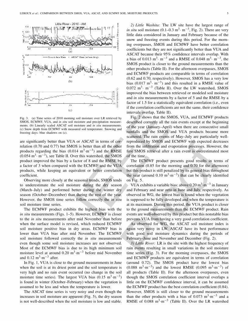
IEEE
Proo
f
LEROUX et al.: COMPARISON BETWEEN SMOS, VUA, ASCAT, AND ECMWF SOIL MOISTURE PRODUCTS 5
(a)
(b)
(c)
Fig. 3. (a) Time series of 2010 morning soil moisture over LR retrieved bySMOS, ECMWF, VUA, and in situ soil moisture and precipitation measure-ments. (b) Linearly scaled ASCAT soil moisture and in situ measurements.(c) Snow depth from ECMWF with measured soil temperature. Snowing andfreezing days: blue shadows on (c).
are significantly better than VUA or ASCAT in terms of cor-relation (0.70 and 0.77) but SMOS is better than all the otherproducts regarding the bias (0.014 m3·m−3) and the RMSE(0.054 m3· m−3), see Table II. Over this watershed, the SMOSproduct improved the bias by a factor of 8 and the RMSE bya factor of 3 when compared with the ECMWF and the VUAproducts, while keeping an equivalent or better correlationcoefficient.
Observing more closely at the seasonal trends, SMOS tendsto underestimate the soil moisture during the dry season(March–July) and performed better during the winter dryseason (October–December) than during the rest of the year.However, the SMOS time series follow correctly the in situsoil moisture time series.
The ECMWF product exhibits the highest bias with thein situ measurements (Figs. 1–5). However, ECMWF is closerto the in situ measurements after mid November than beforewhen the surface model is revised, which reduced ECMWFsoil moisture positive bias in dry areas. ECMWF bias islower than VUA bias after mid November. The ECMWFsoil moisture followed correctly the in situ measurementseven though some soil moisture increases are not observed.Most of the ECMWF bias is due to its high minimum soilmoisture level at around 0.20 m3·m−3 before mid Novemberand 0.12 m3·m−3 after.
In Fig. 1, VUA is close to the ground measurements in Junewhen the soil is at its driest point and the soil temperature isvery high and no rain event occurred (no change in the soilmoisture time series). The largest VUA bias (0.15 m3·m−3)is found in winter (October–February) when the vegetation isassumed to be less and when the temperature is lower.
The ASCAT time series is very noisy and even though theincreases in soil moisture are apparent (Fig. 5), the dry seasonis not well-described when the soil moisture is low and stable.
2) Little Washita: The LW site have the largest range ofin situ soil moisture (0.1–0.3 m3· m−3, Fig. 2). There are verylittle data considered in January and February because of thesnow and freezing events during this period. For the morn-ing overpasses, SMOS and ECMWF have better correlationcoefficients but they are not significantly better than VUA andASCAT because their 95% confidence intervals overlap. Witha bias of 0.013 m3· m−3 and a RMSE of 0.048 m3· m−3, theSMOS product is closer to the ground measurements than theother products (Table II). For the afternoon overpasses, SMOSand ECMWF products are comparable in terms of correlation(0.62 and 0.70, respectively). However, SMOS has a very lowbias (0.017 m3· m−3) and this resulted in a RMSE value of0.072 m3· m−3 (Table II). Over the LW watershed, SMOSimproved the bias between retrieved or modeled soil moistureand in situ measurements by a factor of 5 and the RMSE by afactor of 1.5 for a statistically equivalent correlation (i.e., evenif the correlation coefficients are not the same, their confidenceintervals overlap, Table II).
Fig. 2 shows that the SMOS, VUA, and ECMWF productsdescribed correctly all the rain events except at the beginningof the year (January–April) when there are consecutive smallrainfalls and the SMOS and VUA products became morescattered. The rain events of May–July are particularly well-reproduced by SMOS and ECMWF with expected decreasesfrom the infiltration and evaporation processes. However, thefirst SMOS retrieval after a rain event is overestimated mostof the time.
The ECMWF product presents good results in terms ofcorrelation (0.85 for the morning and 0.70 for the afternoon)but this product is still penalized by its general bias throughoutthe year (around 0.10 m3·m−3) that can be clearly identifiedon Fig. 5.
VUA exhibits a variable bias: above 0.20 m3·m−3 in Januaryand February and near zero in June and July, respectively. Asobserved in WG, the lowest bias is found when the vegetationis supposed to be fully developed and when the temperature isat its maximum. During this period, the VUA product is closerto the ground measurements than the ECMWF product. Rainevents are well-observed by this product but this nonstable biasprevents VUA from having a very good correlation coefficient.
As observed for WG, the ASCAT soil moisture index isagain very noisy in LW. ASCAT have its best performancewith good soil moisture dynamics during the periods ofFebruary–June and November and December (Fig. 2).
3) Little River: LR is the site with the highest frequency ofrain events resulting in small variations in the soil moisturetime series (Fig. 3). For the morning overpasses, the SMOSand ECMWF products are equivalent in terms of correlation(around 0.72). The SMOS product have the lowest bias(0.088 m3·m−3) and the lowest RMSE (0.095 m3·m−3) ofall products (Table II). For the afternoon overpasses, eventhough the SMOS correlation coefficient interval overlaps alittle on the ECMWF confidence interval, it can be assumedthe ECMWF product has the best correlation coefficient (0.84).However, SMOS is still closer to the ground measurementsthan the other products with a bias of 0.073 m3·m−3 and aRMSE of 0.088 m3·m−3 (Table II). Over the LR watershed
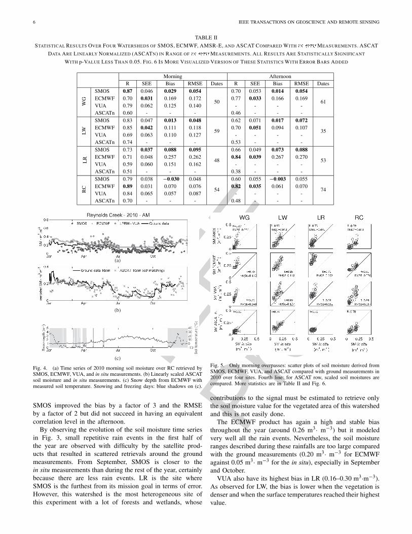
IEEE
Proo
f
6 IEEE TRANSACTIONS ON GEOSCIENCE AND REMOTE SENSING
TABLE II
STATISTICAL RESULTS OVER FOUR WATERSHEDS OF SMOS, ECMWF, AMSR-E, AND ASCAT COMPARED WITH �� ���� MEASUREMENTS. ASCAT
DATA ARE LINEARLY NORMALIZED (ASCATN) IN RANGE OF �� ���� MEASUREMENTS. ALL RESULTS ARE STATISTICALLY SIGNIFICANT
WITH p-VALUE LESS THAN 0.05. FIG. 6 IS MORE VISUALIZED VERSION OF THESE STATISTICS WITH ERROR BARS ADDED
Morning AfternoonR SEE Bias RMSE Dates R SEE Bias RMSE Dates
SMOS 0.87 0.046 0.029 0.054
50
0.70 0.053 0.014 0.054ECMWF 0.70 0.031 0.169 0.172 0.77 0.033 0.166 0.169VUA 0.79 0.062 0.125 0.140 - - - -W
G
ASCATn 0.60 - - - 0.46 - - -
61
SMOS 0.83 0.047 0.013 0.048 0.62 0.071 0.017 0.072
35ECMWF 0.85 0.042 0.111 0.118 0.70 0.051 0.094 0.107VUA 0.69 0.063 0.110 0.127 - - - -LW
ASCATn 0.74 - - -
59
0.53 - - -
SMOS 0.73 0.037 0.088 0.095
48
0.66 0.049 0.073 0.088ECMWF 0.71 0.048 0.257 0.262 0.84 0.039 0.267 0.270VUA 0.59 0.060 0.151 0.162 - - - -L
R
ASCATn 0.51 - - - 0.38 - - -
53
SMOS 0.79 0.038 −0.030 0.048 0.60 0.055 −0.003 0.055
74ECMWF 0.89 0.031 0.070 0.076 0.82 0.035 0.061 0.070VUA 0.84 0.065 0.057 0.087 - - - -R
C
ASCATn 0.70 - - -
54
0.48 - - -
(a)
(b)
(c)
Fig. 4. (a) Time series of 2010 morning soil moisture over RC retrieved bySMOS, ECMWF, VUA, and in situ measurements. (b) Linearly scaled ASCATsoil moisture and in situ measurements. (c) Snow depth from ECMWF withmeasured soil temperature. Snowing and freezing days: blue shadows on (c).
SMOS improved the bias by a factor of 3 and the RMSEby a factor of 2 but did not succeed in having an equivalentcorrelation level in the afternoon.
By observing the evolution of the soil moisture time seriesin Fig. 3, small repetitive rain events in the first half ofthe year are observed with difficulty by the satellite prod-ucts that resulted in scattered retrievals around the groundmeasurements. From September, SMOS is closer to thein situ measurements than during the rest of the year, certainlybecause there are less rain events. LR is the site whereSMOS is the furthest from its mission goal in terms of error.However, this watershed is the most heterogeneous site ofthis experiment with a lot of forests and wetlands, whose
Fig. 5. Only morning overpasses: scatter plots of soil moisture derived fromSMOS, ECMWF, VUA, and ASCAT compared with ground measurements in2010 over four sites. Fourth line: for ASCAT row, scaled soil moistures arecompared. More statistics are in Table II and Fig. 6.
contributions to the signal must be estimated to retrieve onlythe soil moisture value for the vegetated area of this watershedand this is not easily done.
The ECMWF product has again a high and stable biasthroughout the year (around 0.26 m3· m−3) but it modeledvery well all the rain events. Nevertheless, the soil moistureranges described during these rainfalls are too large comparedwith the ground measurements (0.20 m3· m−3 for ECMWFagainst 0.05 m3· m−3 for the in situ), especially in Septemberand October.
VUA also have its highest bias in LR (0.16–0.30 m3·m−3).As observed for LW, the bias is lower when the vegetation isdenser and when the surface temperatures reached their highestvalue.
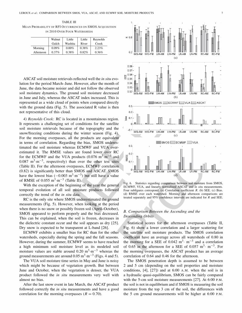
IEEE
Proo
f
LEROUX et al.: COMPARISON BETWEEN SMOS, VUA, ASCAT, AND ECMWF SOIL MOISTURE PRODUCTS 7
TABLE III
MEAN PROBABILITY OF RFI OCCURRENCES ON SMOS ACQUISITION
IN 2010 OVER FOUR WATERSHEDS
Walnut Little Little ReynoldsGulch Washita River Creek
Morning 0.09% 0.00% 0.38% 2.23%Afternoon 0.37% 0.38% 0.82% 0.36%
ASCAT soil moisture retrievals reflected well the in situ evo-lution for the period March–June. However, after the month ofJune, the data became noisier and did not follow the observedsoil moisture dynamics. The ground soil moisture decreasedin June and July, whereas the ASCAT index increased. This isrepresented as a wide cloud of points when compared directlywith the ground data (Fig. 5). The associated R value is thennot representative of this cloud.
4) Reynolds Creek: RC is located in a mountainous region.It represents a challenging set of conditions for the satellitesoil moisture retrievals because of the topography and thesnow/freezing conditions during the winter season (Fig. 4).For the morning overpasses, all the products are equivalentin terms of correlation. Regarding the bias, SMOS underes-timated the soil moisture whereas ECMWF and VUA over-estimated it. The RMSE values are found lower over RCfor the ECMWF and the VUA products (0.076 m3·m−3 and0.087 m3·m−3, respectively) than over the other test sites(Table II). For the afternoon overpasses, ECMWF correlation(0.82) is significantly better than SMOS and ASCAT. SMOShave the lowest bias (−0.003 m3·m−3) but still have a valueof RMSE of 0.055 m3·m−3 (Table II).
With the exception of the beginning of the year the generaltemporal evolution of all soil moisture products followedcorrectly the trend of the in situ data.
RC is the only site where SMOS underestimated the groundmeasurements (Fig. 5). However, when looking at the periodwhen there is no snow or possibly frozen soil (April–October),SMOS appeared to perform properly and the bias decreased.This can be explained, when the soil is frozen, decreases inthe dielectric constant occur and the soil appears as dry [25].Dry snow is expected to be transparent at L-band [26].
ECMWF exhibits a smaller bias for RC than for the otherwatersheds, especially during the spring and the fall seasons.However, during the summer, ECMWF seems to have reacheda high minimum soil moisture level as its modeled soilmoisture values are stable around 0.20 m3·m−3 whereas theground measurements are around 0.05 m3·m−3 (Figs. 4 and 5).
The VUA soil moisture time series in May and June is noisywhich might be because of vegetation growth. But betweenJune and October, when the vegetation is denser, the VUAproduct followed the in situ measurements very well withalmost no bias.
After the last snow event in late March, the ASCAT productfollowed correctly the in situ measurements and have a goodcorrelation for the morning overpasses (R = 0.70).
(a)
(b)
(c)
(d)
Fig. 6. Statistics regarding comparison between soil moisture from SMOS,ECMWF, VUA, and linearly normalized ASCAT and in situ measurements.Four subfigures correspond. (a) Correlation coefficient R. (b) SEE. (c) Bias.(d) RMSE over each watershed. Morning and afternoon comparisons aretreated separately and 95% confidence intervals are indicated for R and SEE.
B. Comparison Between the Ascending and theDescending Orbits
Statistical scores for the afternoon overpasses (Table II,Fig. 6) show a lower correlation and a larger scattering forthe satellite soil moisture products. The SMOS correlationcoefficient have an average across all watersheds of 0.80 inthe morning for a SEE of 0.042 m3· m−3 and a correlationof 0.65 in the afternoon for a SEE of 0.057 m3· m−3. Forthe morning overpasses, the ASCAT product has an averagecorrelation of 0.64 and 0.46 for the afternoon.
The SMOS penetration depth is assumed to be between2 and 5 cm (depending on the soil properties and moistureconditions, [4], [27]) and at 6:00 A.M. when the soil is ina hydraulic quasi-equilibrium, SMOS can be fairly comparedwith the 5-cm soil moisture measurements [27]. At 6:00 P.M.the soil is not in equilibrium and if SMOS is measuring the soilmoisture from the top 3 cm of the soil, the differences withthe 5 cm ground measurements will be higher at 6:00 P.M.

IEEE
Proo
f
8 IEEE TRANSACTIONS ON GEOSCIENCE AND REMOTE SENSING
than at 6:00 A.M. [27] recommended using morning mea-surements when comparing with space observations becauseof the day-time decoupling that could occur in the afternoonbecause of the nonhydraulic equilibrium of the soil. The sameexplanations apply for the ASCAT results at 9:30 A.M. and at9:30 P.M. These results are consistent with the results of [28].
Another possible explanation for these differences betweenthe morning and the afternoon results is still related to thenonequilibrium of the soil and it concerns the assumptions aremade concerning the soil surface temperature. It is assumedthat the soil and the vegetation temperatures are approximatelyequal, which is a fair assumption during the night or earlymorning but during the day, the vegetation temperature isexpected to be closer to the air temperature than to thesoil temperature. This assumption of equal vegetation andeffective soil temperatures can lead to less accurate satellitesoil moisture retrievals in the afternoon.
Regarding SMOS results, one last possibility could be thepresence of RFIs that are only seen during the descendingorbits when the satellite is going in the afternoon fromnorth to south and is pointing in the southwest direc-tion. From the RFI contamination probability maps derivedfrom the mixed polarized acquisitions (real and imaginaryparts [16], [29]), it is possible to compute for each watershedthe mean probability of RFI occurrences (Table III). Exceptover RC, the probability of RFI contamination is higher for theafternoon overpasses even if they are still very low comparedwith highly contaminated regions such as Asia. This differencein RFI contamination between the morning and the afternoonoverpasses might partially explain why SMOS results arebetter in the morning.
V. CONCLUSION
SMOS data were compared with in situ observations andother satellite data and model outputs. SMOS, VUA, ECMWF,and ASCAT soil moisture retrievals were compared with thein situ measurements and intercompared over four differentsites in the U.S. under various climate conditions and soilcharacteristics.
Over the four test sites, no specific product had a sig-nificantly better correlation with the ground measurements.Since this paper only covers the year 2010, 35–74 commondates were considered to compute the statistics and resultedin substantial confidence intervals that made all productsequivalent in terms of correlation. The statistical parametersused to differentiate the four data sets were the SEE, thebias, and logically the RMSE. Over most of the watersheds,ECMWF had a significantly lower SEE (0.039 m3· m−3 inaverage) than SMOS (0.049 m3· m−3 in average) and VUA(0.063 m3· m−3 for the morning only), representing a lessscattered data set. ECMWF soil moisture time evolution wasvery close to the ground measurements with clear identifica-tions of the rainfall events and the soil drainage afterward.However, SMOS had clearly the lowest bias with an averageof 0.032 m3· m−3 whereas ECMWF had a mean bias of0.150 m3· m−3 and VUA of 0.129 m3· m−3. SMOS also hadthe lowest RMSE over all the sites except RC. SMOS had
a mean RMSE of 0.064 m3· m−3 whereas ECMWF had amean RMSE of 0.156 m3· m−3 and VUA of 0.129 m3· m−3
(for the morning only). Therefore, although the SMOS missionaccuracy objective of 0.040 m3· m−3 was not reached overthese four watersheds in 2010, SMOS improved the totalRMSE by a factor of at least 2 on average in 2010 for anequivalent correlation compared with the other soil moistureproducts.
The time series analysis revealed a positive constant biasin the ECMWF data set: 0.17/0.10/ 0.26/0.07 m3· m−3,respectively for the WG/LW/LR/RC watersheds. Even aftermid-November when the surface model and analysis wererevised, this bias was still present over all the watersheds buthad decreased over WG (data after mid-November were notconsidered in the statistical results). Despite very good corre-lation coefficients, this minimum level was a major obstacle inusing ECMWF for the four test sites. VUA also had a bias butwas not constant and appeared to evolve with the seasons. Thebias was higher when the vegetation and the soil temperaturewere low (during winter) and tended to decrease when thevegetation was supposed to be denser and the soil temperatureincreasing to its maximum in the summer, resulting in a quasi-null bias. This evolution of the VUA bias throughout the yearwas assumed to be linked to a physical parameter such as thevegetation or the temperature since it evolved with the seasonsand because the AMSR-E frequencies (6.9 and 10.7 GHz)were more sensitive to the vegetation layer than SMOS at1.4 GHz. It was also possible that this bias was due to the soileffective temperature that was modeled through the 36-GHzbrightness temperature or to another assumption that was madein the VUA algorithm. The ASCAT soil moisture index wasvery noisy in comparison with the other products and eventhough some rain events were obvious in the retrievals, thein situ soil moisture dynamics were not well-represented forany of the watersheds. Active microwave observations werevery sensitive to surface roughness and WG, for example,had sandy soils with significant amount of gravel. These soilcharacteristics resulted in a greater surface roughness whichcould explain partially the poor results of ASCAT.
The comparison of the statistical performances of theproducts between the morning and the afternoon revealedthat the ECMWF model did not show significant differenceswhereas the satellite SMOS and ASCAT products showedseveral differences: R = 0.80/0.65, SE E = 0.042/0.057 m3·m−3, bias = 0.040/0.027 m3· m−3, RMSE =0.061/0.067 m3· m−3 for SMOS, and R = 0.64/0.46 forASCAT (A.M./P.M. in average over the four watersheds).These differences in performance can be explained that inthe morning, the soil was in hydraulic quasi-equilibrium. Onthe other hand for the afternoon, this comparison might notbe as correct as for the morning. Another explanation couldbe the inaccurate modeling of the soil and the vegetationtemperatures in the retrieval algorithm. They were assumedto be equal and this assumption might not be true in theafternoon when the vegetation temperature was expected tobe closer to the air temperature than to the soil temperature.The last possible explanation for SMOS performancedifference concerned the RFI. The occurrence probabilities of

IEEE
Proo
f
LEROUX et al.: COMPARISON BETWEEN SMOS, VUA, ASCAT, AND ECMWF SOIL MOISTURE PRODUCTS 9
RFI in 2010 were higher in the afternoon than in the morningexcept over RC.
The results of this paper concur with the different studiesthat were realized in the frame of the SMOS soil moistureproduct validation [11], [12], [14], [30]. SMOS soil moistureretrievals were already very close to the ground measurementsbut need to be improved to meet its scientific goal of an errorless than 0.04 m3· m−3. In this perspective, a new versionof the level 2 soil moisture processor (v5.51) was already inplace since March 2012 and allowed to switch between theDobson and the Mironov constant dielectric model and thisversion showed promising first results.
The main advantage in comparing satellite products wasthe possibility of comparing with global coverage and furtherstudies will be developed in this direction in the near future.
ACKNOWLEDGMENT
The authors would like to thank the U.S. Department ofAgriculture (Agricultural Research Service) for providing theground data.
REFERENCES
[1] “Implementation plan for the global observing system for climate insupport of the UNFCCC,” World Meteorological Organ., Intergovern.Oceanogr. Commission, United Nations Environ. Progr., InternationalCouncil Science, Geneva, Switzerland, Tech. Rep. 1244, 2010.
[2] M. Drusch, “Initializing numerical weather predictions models withsatellite derived surface soil moisture: Data assimilation experimentswith ECMWF’s integrated forecast system and the TMI soil moisturedata set,” J. Geophys. Res., vol. 113, no. D3, p. D03102, Feb. 2007.
[3] H. Douville and F. Chauvin, “Relevance of soil moisture for seasonalclimate predictions: A preliminary study,” Climate Dynamics, vol. 16,nos. 10–11, pp. 719–736, Oct. 2000.
[4] Y. Kerr, P. Waldteufel, J. Wigneron, S. Delwart, F. Cabot, J. Boutin,M. Escorihuela, J. Font, N. Reul, C. Gruhier, S. Juglea, M. Drinkwater,A. Hahne, M. Martin-Neira, and S. Mecklenburg, “The SMOS mission:New tool for monitoring key elements of the global water cycle,” Proc.IEEE, vol. 98, no. 5, pp. 666–687, May 2010.
[5] D. Entekhabi, E. Njoku, P. E. O. Neill, K. Kellogg, W. Crow, W. Edel-stein, J. Entin, S. Goodman, T. Jackson, J. Johnson, J. Kimball, J. Piep-meier, R. Koster, N. Martin, K. McDonald, M. Moghaddam, S. Moran,R. Reichle, J. Shi, M. Spencer, S. Thurman, L. Tsang, and J. Zyl, “Thesoil moisture active passive (smap) mission,” Proc. IEEE, vol. 98, no. 5,pp. 704–716, May 2010.
[6] Y. Kerr, P. Waldteufel, J. Wigneron, J. Martinuzzi, J. Font, andM. Berger, “Soil moisture retrieval from space: The soil moisture andocean salinity (SMOS) mission,” IEEE Trans. Geosci. Remote Sens.,vol. 39, no. 8, pp. 1729–1735, Aug. 2001.
[7] M. Owe, R. de Jeu, and J. Walker, “A methodology for surface soilmoisture and vegetation optical depth retrieval using the microwavepolarization difference index,” IEEE Trans. Geosci. Remote Sens.,vol. 39, no. 8, pp. 1643–1654, Aug. 2001.
[8] E. Njoku, T. Jackson, V. Lakshmi, T. Chan, and S. Nghiem, “Soilmoisture retrieval from ASMR-E,” IEEE Trans. Geosci. Remote Sens.,vol. 41, no. 2, pp. 215–229, Feb. 2003.
[9] L. Li, P. Gaiser, B. Gao, R. Bevilacqua, T. Jackson, E. Njoku, C. Rüdiger,J. Calvet, and R. Bindlish, “Windsat global soil moisture retrievaland validation,” IEEE Trans. Geosci. Remote Sens., vol. 48, no. 5,pp. 2224–2241, May 2010.
[10] V. Naeimi, K. Scipal, Z. Bartalis, and S. H. W. Wagner, “An improvedsoil moisture retrieval algorithm for ERS and METOP scatterometerobservations,” IEEE Trans. Geosci. Remote Sens., vol. 47, no. 7,pp. 1999–2013, Jul. 2009.
[11] A. A. Bitar, D. Leroux, Y. Kerr, O. Merlin, P. Richaume, A. Sahoo, andE. Wood, “Evaluation of SMOS soil moisture products over continentalU.S. Using SCAN/SNOTEL network,” IEEE Trans. Geosci. RemoteSens., vol. 50, no. 5, pp. 1572–1586, May 2012.
[12] T. Jackson, R. Bindlish, M. Cosh, T. Zhao, P. Starks, D. Bosch,M. Seyfried, S. Moran, Y. Kerr, and D. Leroux, “Validation of soilmoisture ocean salinity (SMOS) soil moisture over watershed networksin the U.S.,” IEEE Trans. Geosci. Remote Sens., vol. 50, no. 5,pp. 1530–1543, May 2012.
[13] J. Wigneron, Y. Kerr, P. Waldteufel, K. Saleh, M. Escorihuela,P. Richaume, P. Ferrazzoli, P. de Rosnay, R. Gurney, J. Calvet,J. Grant, M. Guglielmetti, B. Hornbuckle, C. Mätzler, T. Pellarin, andM. Schwank, “L-band microwave emission of the biosphere (L-MEB)model: Description and calibration against experimental data sets overcrop fields,” Remote Sens. Environ., vol. 107, no. 4, pp. 639–655,Apr. 2007.
[14] Y. Kerr, P. Waldteufel, P. Richaume, J. Wigneron, P. Ferrazzoli, A. Mah-moodi, A. Al Bitar, F. Cabot, C. Gruhier, S. Juglea, D. Leroux,A. Mialon, and S. Delwart, “The SMOS soil moisture retrieval algo-rithm,” IEEE Trans. Geosci. Remote Sens., vol. 50, no. 5, pp. 1384–1403,May 2012.
[15] V. Masson, J.-L. Champeau, F. Chauvin, C. Meriguet, and R. Lacaze,“A global data base of land surface parameters at 1-km resolutionin meteorological and climate models,” J. Climate, vol. 16, no. 9,pp. 1261–1282, May 2003.
[16] “Algorithm theoretical basis document,” Tech. Rep. 3.d, CESBIO,Toulouse, France, IPSL, Paris, France, INRA-EPHYSE, Bordeaux,France, Reading University, Reading, England, Tor Vergata University,Rome, Italy, 2010.
[17] D. Carr, R. Kahn, K. Sahr, and T. Olsen, “Isea discrete global grids,”Stat. Comput. Stat. Graph. Newlett., vol. 8, nos. 2–3, pp. 31–39, 1997.
[18] W. Wagner, G. Lemoine, and H. Rott, “A method for estimating soilmoisture from ERS scatterometer and soil data,” Remote Sens. Environ.,vol. 70, no. 2, pp. 191–207, Nov. 1999.
[19] “AMSR-E data users handbook,” Japan Aerospace Exploration Agency(JAXA), Washington, DC, USA, Tech. Rep. NCX-030021, Mar. 2006.
[20] C. Gruhier, P. de Rosnay, Y. Kerr, E. Mougin, E. Ceschia, J. Calvet, andP. Richaume, “Evaluation of AMSR-E soil moisture product based onground measurements over temperate and semi-arid regions,” Geophys.Res. Lett., vol. 35, no. 10, p. L10405, May 2008.
[21] C. Rudiger, J. C. Calvet, C. Gruhier, T. Holmes, R. de Jeu, and W. Wag-ner, “An intercomparison of ERS-Scat and AMSR-E soil moistureobservations with model simulations over france,” Amer. Meteorol. Soc.,vol. 10, no. 2, pp. 431–447, Apr. 2009.
[22] C. Draper, J. Walker, P. Steinle, R. de Jeu, and T. Holmes, “An evalu-ation of AMSR-E derived soil moisture over Australia,” Remote Sens.Environ., vol. 113, no. 4, pp. 703–710, Apr. 2009.
[23] C. Gruhier, P. de Rosnay, S. Hasenauer, T. Holmes, R. de Jeu, Y. Kerr,E. Mougin, E. Njoku, F. Timouk, W. Wagner, and M. Zribi, “Soilmoisture active and passive microwave products: Intercomparison andevaluation over a sahelian site,” Hydrol. Earth Syst. Sci., vol. 14, no. 1,pp. 141–156, Jan. 2010.
[24] T. Jackson, M. Cosh, R. Bindlish, P. Starks, D. Bosch, M. Seyfried,D. Goodrich, M. Moran, and J. Du, “Validation of advancedmicrowave scanning radiometer soil moisture products,” IEEETrans. Geosci. Remote Sens., vol. 48, no. 12, pp. 4256–4272,Dec. 2010.
[25] C. Matzler, “Passive microwave signatures of landscapes in winter,”Meteorol. Atmospheric Phys., vol. 54, nos. 1–4, pp. 241–260, 1994.
[26] R. Armstrong and M. Brodzik, “A twenty year record of global snowcover fluctuations derived from passive microwave remote sensing data,”in Proc. 5th Conf. Polar Meteorol. Oceanography, Amer. Meteorol. Soc.,Dallas, TX, USA, 1999, pp. 113–117.
[27] T. Jackson, “Profile soil moisture from space measurements,” J. Irrigat.Drainage Divis., ASCE, vol. 106, pp. 81–92, Mar. 1980.
[28] C. Albergel, C. Rüdiger, D. Carrer, J. Calvet, N. Fritz, V. Naeimi,Z. Bartalis, and S. Hasenauer, “An evaluation of ascat surfacesoil moisture products with in-situ observations in southwesternfrance,” Hydrol. Earth Syst. Sci., vol. 13, no. 2, pp. 115–124,2009.
[29] R. Oliva, E. Daganzo-Eusebio, Y. Kerr, S. Mecklenburg,S. Nieto, P. Richaume, and C. Gruhier, “SMOS radio frequencyinterference scenario: Status and actions taken to improve theRFI environment in the 1400–1427 MHz passive band,” IEEETrans. Geosci. Remote Sens., vol. 50, no. 5, pp. 1427–1439,May 2012.
[30] C. Albergel, P. de Rosnay, C. Gruhier, J. Munoz-Sabater, S. H. L. Isak-sen, Y. Kerr, and W. Wagner, “Evaluation of remotely sensedand modelled soil moisture products using global ground-based insitu observations,” Remote Sens. Environ., vol. 118, pp. 215–226,Mar. 2012.

IEEE
Proo
f
10 IEEE TRANSACTIONS ON GEOSCIENCE AND REMOTE SENSING
DELPHINE J. Leroux received the M.S. degreein applied mathematics from Institut National desSciences Appliquees, Toulouse, France, in 2009,and the Ph.D. degree in spatial hydrology fromUniversite Paul Sabatier, Toulouse, France, in 2012.
She was with the Centre d’Etudes Spatiales de laBiosphere, Toulouse, from 2009 to 2012, where sheworked on the validation of the soil moisture andocean salinity soil moisture product at the local andthe global scales by using statistical and physicalmethods. Currently, she is with the Jet Propulsion
Laboratory, Pasadena, CA, USA, where she works on the soil moisture activepassive mission.
Yann H. Kerr (M’88–SM’01–F’13) received theEngineering degree from Ecole Nationale Suprieurede l’Aronautique et de l’Espace, the M.Sc. degree inelectronics and electrical engineering from GlasgowUniversity, Glasgow, U.K., and the Ph.D. degree inAstrophysique Gophysique et Techniques Spatiales,Universit Paul Sabatier, Toulouse, France.
He is currently the Director of Centre dEtudesSpatiales de la BIOsphre, Toulouse, France. He wasan Earth Observation System Principal Investiga-tor (interdisciplinary investigations) and a Principal
Investigator and precursor of the use of the scatterometer over land. In 1990,he started to work on the interferometric concept applied to passive microwaveearth observation and was subsequently the science lead on the microwaveimaging radiometer with aperture synthesis project for the European SpaceAgency. In 1997, he proposed the SMOS Mission, the natural outcome of theprevious MIRAS work. He is currently involved in the exploitation of SMOSdata, in the calibration/validation activities and related level 2 soil moistureand level 3 and 4 developments. He is working on the SMOS next concept.His current research interests include theory and techniques for microwave andthermal infrared remote sensing of the Earth, with emphasis on hydrology,and water resources management.
Dr. Kerr was a recipient of the World Meteorological Organization 1stprize (Norbert Gerbier), the USDA Secretary’s Team Award for Excellence(Salsa Program), the Geoscience and Remote Sensing Society certificateof recognition for leadership in development of the first synthetic aperturemicrowave radiometer in space and success of the SMOS mission, and theDistinguished Lecturer for GRSS.
Ahmad Al Bitar received the M.E. degree in civilengineering from INSA-Lyon, Villeurbanne, France,in 2003, and the Ph.D. degree in hydrogeologyfrom Institut National Polytechnique de Toulouse,Toulouse, France, in 2006. His thesis work focuseson numerical modeling in stochastic porous media.
He joined CESBIO, Toulouse, France, in 2006. Hiscurrent research interests include integrated hydro-logical modeling and assimilation of remote sensingdata.
Rajat Bindlish (S’98–AM’99–M’03–SM’05)received the B.S. degree in civil engineeringfrom the Indian Institute of Technology, Bombay,India, in 1993, and the M.S. and Ph.D. degreesin civil engineering from The Pennsylvania StateUniversity, University Park, PA, USA, in 1996 and2000, respectively.
He is currently with the USDA AgriculturalResearch Service, Hydrology and Remote SensingLaboratory, Beltsville, MD, USA. He is currentlyworking on soil moisture estimation from microwave
sensors and their subsequent application in land surface hydrology. Hiscurrent research interests include the application of microwave remotesensing in hydrology.
Thomas J. Jackson (SM’96–F’02) received thePh.D. degree from the University of Maryland, Col-lege Park, MD, USA, in 1976.
He is a Research Hydrologist with the U.S. Depart-ment of Agriculture, Agricultural Research Service,Hydrology and Remote Sensing Laboratory. Hisresearch involves the application and developmentof remote sensing technology in hydrology andagriculture, primarily microwave measurement ofsoil moisture. He has been a member of the Sci-ence and Validation Teams of the Aqua, ADEOS-II
(Advanced Earth Observing Satellite), Radarsat, Oceansat-1, Envisat, ALOS(Advanced Land Observing Satellite), SMOS, Aquarius, GCOM-W (GlobalChange Observation Mission - Water), and SMAP remote sensing satellites.
Dr. Jackson is a Fellow of the Society of Photo-Optical InstrumentationEngineers, the American Meteorological Society, and the American Geophys-ical Union. In 2003, he was a recipient of the William T. Pecora Award(NASA and Department of Interior) for outstanding contributions towardunderstanding the Earth by means of remote sensing and the AmericanGeophysical Union Hydrologic Sciences Award for outstanding contributionsto the science of hydrology. He was a recipient of the IEEE Geoscience andRemote Sensing Society Distinguished Achievement Award in 2011.
Beatrice Berthelot received the Ph.D. degree inoceanography to estimate the ocean primary produc-tion using ocean color data in 1991.
She has considerable expertise in satellite remotesensing both over ocean and land. She was a Post-Doctoral with the California Space Institute, CA,USA, and Scripps Institution for Oceanography,USA. From 1993 to 2000, she was a ResearchEngineer with the Centre dEtude Spatiales de laBIOsphere, Toulouse, France. She developed dataprocessing chains for long time series of AVHRR
satellite dataset from 1983 to 1995, including calibration monitoring,atmospheric corrections, cloud and snow detection, and associated qualityflags. She developed the atmospheric correction algorithm scheme whichis applied at Centre de Traitement des Images VEGETATION. From 2000to 2006, she was the Terrestrial Biosphere Group Leader with NOVELTIS,Toulouse. She worked on multiple projects for CNES, ESA and EC, such asCYCLOPES FP5, from 2003 to 2006, the development of MERIS algorithmover land including atmosphere products and vegetation products ESA, from2004 to 2006, GLOBCOVER for the assessment and development of thecloud mask for MERIS. She worked on SMOS soil moisture simulations andretrieval using neural networks. She joined VEGA Technologies in 2008 asa Leader of Scientific Algorithms Group, when she worked on radiometriccalibration (test sites project, ESRIN), and managed the development of theapplication dedicated to the absolute radiometric calibration of HR satellites(ROSAS, 2011). She was involved in the development of the Level 2 Sentinel2 product and algorithm definition, for the atmospheric correction algorithmdevelopment and pixel classification definitions. Since October 2011, she hasbeen with MAGELLIUM in the data and signal processing department. Sheis the Project Manager for the development of vicarious calibration methodinside the DIMITRI ESA software. She has large expertise on radiativetransfer in the atmosphere.
Gautier Portet received an Associate degree insoftware development.
He is a Software Developer with Telespazio,France, and has been working on the Geoland2 SoilWater Index processing chain.