COMPARISON BETWEEN ARTIFICIAL NEURAL NETWORKS … · COMPARISON BETWEEN ARTIFICIAL NEURAL NETWORKS...

COMPARISON BETWEEN ARTIFICIAL NEURAL NETWORKS AND MAXIMUM LIKELIHOOD... 339

R. Bras. Ci. Solo, 37:339-351, 2013

COMPARISON BETWEEN ARTIFICIAL NEURAL NETWORKS

AND MAXIMUM LIKELIHOOD CLASSIFICATION IN DIGITAL

SOIL MAPPING(1)

César da Silva Chagas(2), Carlos Antônio Oliveira Vieira(3) & Elpídio Inácio Fernandes

Filho(4)

SUMMARY

Soil surveys are the main source of spatial information on soils and have a

range of different applications, mainly in agriculture. The continuity of this activity

has however been severely compromised, mainly due to a lack of governmental

funding. The purpose of this study was to evaluate the feasibility of two different

classifiers (artificial neural networks and a maximum likelihood algorithm) in the

prediction of soil classes in the northwest of the state of Rio de Janeiro. Terrain

attributes such as elevation, slope, aspect, plan curvature and compound

topographic index (CTI) and indices of clay minerals, iron oxide and Normalized

Difference Vegetation Index (NDVI), derived from Landsat 7 ETM+ sensor imagery,

were used as discriminating variables. The two classifiers were trained and validated

for each soil class using 300 and 150 samples respectively, representing the

characteristics of these classes in terms of the discriminating variables. According

to the statistical tests, the accuracy of the classifier based on artificial neural

networks (ANNs) was greater than of the classic Maximum Likelihood Classifier

(MLC). Comparing the results with 126 points of reference showed that the resulting

ANN map (73.81 %) was superior to the MLC map (57.94 %). The main errors when

using the two classifiers were caused by: a) the geological heterogeneity of the area

coupled with problems related to the geological map; b) the depth of lithic contact

and/or rock exposure, and c) problems with the environmental correlation model

used due to the polygenetic nature of the soils. This study confirms that the use of

terrain attributes together with remote sensing data by an ANN approach can be a

tool to facilitate soil mapping in Brazil, primarily due to the availability of low-cost

remote sensing data and the ease by which terrain attributes can be obtained.

Index terms: terrain attributes; neural networks; maximum likelihood.

(1) Received for publication on July 18, 2012 and approved on February 28, 2013.(2) Pesquisador A da Embrapa Solos. Rua Jardim Botânico, 1024. CEP 22460-000 Rio de Janeiro (RJ). E-mail: [email protected];

[email protected](3) Professor do Departamento de Geociências, Universidade Federal de Santa Catarina - UFSC. Caixa-Postal 476. CEP 88040-900

Florianópolis (SC). E-mail: [email protected](4) Professor do Departamento de Solos, Universidade Federal de Viçosa - UFV. Av. P.H. Rolfs, s/n. CEP 36570-000 Viçosa (MG). E-mail:

[email protected]

César da Silva Chagas et al.

R. Bras. Ci. Solo, 37:339-351, 2013

340

RESUMO: COMPARAÇÃO ENTRE REDES NEURAIS ARTIFICIAIS ECLASSIFICAÇÃO POR MÁXIMA VEROSSIMILHANÇA NOMAPEAMENTO DIGITAL DE SOLOS

O levantamento de solos é a principal fonte de informação espacial sobre solos paradiferentes usos, principalmente o uso agrícola. No entanto, a continuidade dessa atividade temsido grandemente comprometida, principalmente pela escassez de recursos financeiros. O objetivodeste estudo foi avaliar a eficiência da utilização de dois classificadores distintos (redes neuraisartificiais - RNAs e o algoritmo da máxima verossimilhança - Maxver) na predição de classesde solos em uma área na região noroeste do Estado do Rio de Janeiro. As variáveisdiscriminantes usadas incluem atributos do terreno, como elevação, declividade, aspecto, planode curvatura e índice topográfico combinado (CTI) e índices clay minerals, iron oxide e devegetação NDVI, derivados de uma imagem do sensor ETM+ do LANDSAT 7. Para otreinamento e a validação dos classificadores, foram utilizadas, respectivamente, 300 e 150amostras por classe de solo, representativas das características dessas classes, com relação àsvariáveis discriminantes utilizadas. De acordo com os testes estatísticos realizados, oclassificador com base na RNA produziu maior exatidão do que o classificador clássico damáxima verossimilhança (Maxver). A comparação com 126 pontos de referência coletados nocampo evidenciou que o mapa produzido pela RNA teve desempenho superior (73,81 %) aomapa produzido pelo algoritmo Maxver (57,94 %). As principais causas de erros detectadasna utilização desses classificadores foram: a heterogeneidade geológica da área aliada aproblemas no mapa geológico utilizado; profundidade do contato lítico e, ou, exposição darocha; e problemas com o modelo de correlação ambiental utilizado em razão da naturezapoligenética dos solos. Os resultados obtidos permitem inferir que a utilização de atributos doterreno juntamente com dados de sensoriamento remoto em uma abordagem por RNAs podecontribuir para facilitar o mapeamento de solos no Brasil, principalmente por causa dadisponibilidade de dados de sensores remotos a custos mais baixos e da facilidade de obtençãodos atributos do terreno.

Termos de indexação: atributos do terreno; redes neurais artificiais; máxima verossimilhança.

INTRODUCTION

Soil survey is one of the main sources of spatialinformation on soils and has a wide range of uses.The qualitative landscape approach used in thesesurveys based on the interpretation of aerialphotographs has however been criticized, for notallowing an understanding of the quantitativerelationships between the shape of the land surface andthe soils and their properties (McBratney et al., 2000).

Therefore, various quantitative methods(McBratney et al., 2003) have been developed over thelast few years to describe, classify and study patternsof spatial distribution in soils. These methods aregrouped together in an emerging field of soil scienceknown as pedometrics (McBratney et al., 2000). Thisway of mapping soils digitally involves the quantitativeprediction of soils and their properties using measuredand/or observed and auxiliary data representingfactors of soil formation. Various techniques have beenused to predict soil properties and/or classes, such askriging (Brus & Heuvelink, 2007; Weindorf & Zhu,2010), multiple logistic regression (Hengl et al., 2007;Ten Caten et al., 2011), decision trees (Elnaggar &Noller, 2010; Giasson et al., 2011), and artificial neuralnetworks (Behrens et al., 2005; Boruvka & Penizek,2007; Chagas et al., 2010), among others.

The main advantages of artificial neural networks(ANNs) are an efficient handling of large quantitiesof data and their capacity for generalization.Furthermore, they require no specific type of datadistribution, unlike the traditional parametricstatistical approach, which implies normal datadistribution, and allow the manipulation of data fromdifferent sources, with different levels of precision andnoise (Atkinson & Tatnall, 1997; Benediktsson &Sveinsson, 1997).

In soil science, ANNs have already been used tomap soil properties, mainly (McBratney et al., 2003).However, their application in the mapping of soilclasses is less common and has been reported in onlya few studies. Zhu (2000) used ANNs to populate asoil similarity model constructed to represent soillandscape as spatial continua. In this study, a set ofsoil formative factors were used as input data for thenetwork, and the map derived by this approach wasmore detailed and superior to that derived from aconventional soil map.

An approach to the digital mapping of soil classesbased on ANNs was developed by Behrens et al. (2005),using 69 terrain attributes, 53 geological units andthree types of land use, extracted from existing mapsand databases. In general, this approach proved fairlysatisfactory, saved time, reduced financial costs and


R. Bras. Ci. Solo, 37:339-351, 2013

provided reliable results, with an average accuracy ofthe evaluated soil units of over 92 % for both trainingand validation. Boruvka & Penizek (2007) used ANNsfor the mapping of soil classes with data of pH, claylevels and textural gradient from pre-existing soilsurveys, as well as data on elevation, aspect and plancurvature as discriminating variables. The resultsdemonstrated differences in the allocation of the soilclasses.

In Brazil, the use of ANNs for the prediction ofsoil class was described by Chagas et al. (2010, 2011),who demonstrated the efficiency of this approach indigital soil mapping. Despite the growing use in recentyears, there is still an enormous lack of studiesinvolving digital soil mapping in Brazil, and mainlywith a view to the selection of predictors, soil samplingtechniques, evaluation of prediction methods (MLC,ANNs, decision trees, multiple logistic regressions,etc.), validation methods, and even the evaluation ofthe different environmental conditions in the country.

In this context, this study differs from previous workin its objective to compare the efficiency of the twoprediction methods (ANNs and MLC) for digital soilmapping, using terrain attributes derived from a digitalelevation model (DEM) and data from an orbital remotesensor (Landsat 7), to evaluate the real possibility ofusing these approaches in medium-scale soil surveys.

MATERIALS AND METHODS

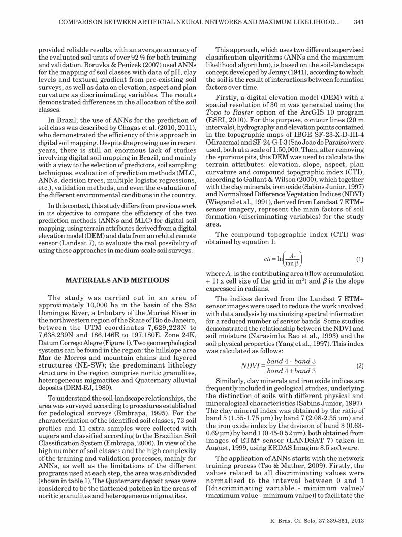
The study was carried out in an area ofapproximately 10,000 ha in the basin of the SãoDomingos River, a tributary of the Muriaé River inthe northwestern region of the State of Rio de Janeiro,between the UTM coordinates 7,629,223N to7,638,239N and 186,146E to 197,180E, Zone 24K,Datum Córrego Alegre (Figure 1). Two geomorphologicalsystems can be found in the region: the hillslope areaMar de Morros and mountain chains and layeredstructures (NE-SW); the predominant lithologystructure in the region comprise noritic granulites,heterogeneous migmatites and Quaternary alluvialdeposits (DRM-RJ, 1980).

To understand the soil-landscape relationships, thearea was surveyed according to procedures establishedfor pedological surveys (Embrapa, 1995). For thecharacterization of the identified soil classes, 73 soilprofiles and 11 extra samples were collected withaugers and classified according to the Brazilian SoilClassification System (Embrapa, 2006). In view of thehigh number of soil classes and the high complexityof the training and validation processes, mainly forANNs, as well as the limitations of the differentprograms used at each step, the area was subdivided(shown in table 1). The Quaternary deposit areas wereconsidered to be the flattened patches in the areas ofnoritic granulites and heterogeneous migmatites.

This approach, which uses two different supervisedclassification algorithms (ANNs and the maximumlikelihood algorithm), is based on the soil-landscapeconcept developed by Jenny (1941), according to whichthe soil is the result of interactions between formationfactors over time.

Firstly, a digital elevation model (DEM) with aspatial resolution of 30 m was generated using theTopo to Raster option of the ArcGIS 10 program(ESRI, 2010). For this purpose, contour lines (20 mintervals), hydrography and elevation points containedin the topographic maps of IBGE SF-23-X-D-III-4(Miracema) and SF-24-G-I-3 (São João do Paraíso) wereused, both at a scale of 1:50,000. Then, after removingthe spurious pits, this DEM was used to calculate theterrain attributes: elevation, slope, aspect, plancurvature and compound topographic index (CTI),according to Gallant & Wilson (2000), which togetherwith the clay minerals, iron oxide (Sabins Junior, 1997)and Normalized Difference Vegetation Indices (NDVI)(Wiegand et al., 1991), derived from Landsat 7 ETM+sensor imagery, represent the main factors of soilformation (discriminating variables) for the studyarea.

The compound topographic index (CTI) wasobtained by equation 1:

(1)

where As is the contributing area ((flow accumulation+ 1) x cell size of the grid in m2) and β is the slopeexpressed in radians.

The indices derived from the Landsat 7 ETM+sensor images were used to reduce the work involvedwith data analysis by maximizing spectral informationfor a reduced number of sensor bands. Some studiesdemonstrated the relationship between the NDVI andsoil moisture (Narasimha Rao et al., 1993) and thesoil physical properties (Yang et al., 1997). This indexwas calculated as follows:

(2)

Similarly, clay minerals and iron oxide indices arefrequently included in geological studies, underlyingthe distinction of soils with different physical andmineralogical characteristics (Sabins Junior, 1997).The clay mineral index was obtained by the ratio ofband 5 (1.55-1.75 µm) by band 7 (2.08-2.35 µm) andthe iron oxide index by the division of band 3 (0.63-0.69 µm) by band 1 (0.45-0.52 µm), both obtained fromimages of ETM+ sensor (LANDSAT 7) taken inAugust, 1999, using ERDAS Imagine 8.5 software.

The application of ANNs starts with the networktraining process (Tso & Mather, 2009). Firstly, thevalues related to all discriminating values werenormalised to the interval between 0 and 1[(discriminating variable - minimum value)/(maximum value - minimum value)] to facilitate the


R. Bras. Ci. Solo, 37:339-351, 2013

342

training process and avoid ANN saturation, as verylarge values can hamper the problem solution(saturation of the transfer functions could hinder theconvergence of the network). Furthermore, efforts weremade to prevent large variations in unimportantvariables from inhibiting small variations in othermore important variables.

The Java Neural Network Simulator was used forthe classification by ANNs, based on the StuttgartNeural Network Simulator 4.2 Kernel (Zell et al.,1996), and an applicable algorithm (funcpow) developedby Vieira (2000) for the classification by a MaximumLikelihood Classifier (MLC).

Two sets of independent stratified samples werecollected from the areas containing profiles

considered to be representative of each soil class,one for the training process and the other forvalidation of the two classifiers. In this way, effortswere made to represent the characteristics of eachone in relation to the discrimination variables used(elevation, slope, aspect, plan curvature, CTI index,clay mineral index, iron oxide index, and NDVIindex). It should be highlighted that the soil classesdiffered in relation to one or more of thediscriminating variables. The training samples wereused so that the classifiers could establishrelationships between the discriminating variables(input data) and the soil classes (output data)through a learning process. The validation sampleswere then used to test this relationship by statisticalmeans.

Figure 1. Localization of the study area in the basin of the São Domingos River (in the northwest of Rio de

Janeiro state) and elevation profile across the diagonal line A-B, showing the geomorphological domains

and main lithology of the area.


R. Bras. Ci. Solo, 37:339-351, 2013

The training samples for both classifiers consistedof 300 samples or pixels per class, i.e., 3,600 samplesfor Area 1 and 3,000 samples for Area 2. The numberof validation samples was limited to 50 % of the numberof training samples (150 samples or pixels per class),with 1,800 samples for Area 1 and 1,500 samples forArea 2, according to Zhu (2000).

In the training step, 10 ANN architectures weretested, which differed only in terms of the number ofneurons in the internal layer (3, 5, 6, 7, 8, 9, 10, 15,20, and 25 neurons). All of these had the same numberof neurons in the input layer (number ofdiscriminating variables) and in the output layer (12soil classes for Area 1 and 10 for Area 2). The learningalgorithm used was the backpropagation method, withrandom allocation of interneuron weights between -0.5 and 0.5 and a learning rate of 0.2, involving 10,000learning cycles.

The results were evaluated through statisticalmeans using the Kappa coefficient and overallclassification accuracy, derived from a confusionmatrix (Congalton & Green, 1999) from the validationsamples. In this way, the ANN architecture obtainingthe best result for the Kappa coefficient was selectedfor the prediction of the soil classes.

A statistical test to verify the significance of thedifferences between two or more classifiers (represented

by their respective confusion matrices) using Kappacoefficient analysis is proposed as an alternativeapproach for the comparison of independent confusionmatrices. In this way, a significance matrix wasgenerated using the results of the statistical tests forthe chosen ANN and the classification with MLC,using the Kappa values and Kappa variance betweenthe classifications, by means of the Z statistical test.The formula to test the significance between twoindependent Kappa coefficients (Z test) is given in thefollowing equation:

(3)

Where Ka1 and Ka2 are the two Kappa coefficientsthat are being compared (Congalton & Mead, 1986)and var is the variance of the Kappa coefficient (Ka).

Thus, the Z test firstly verifies if the classificationdiffers from a causal classification. In other words, ifZ calculated < Zα/2 tabulated, the classification issignificantly better than a random classification,where α/2 is the confidence level of the Z test and thenumber of degrees of freedom is assumed to be infinite.In a second analysis, the test verifies if there is asignificant difference between the Kappa valuesresulting from the evaluation by the differentclassifiers. Values < than 1.96 (95 % confidence level)

Symbol Soil class No. profiles and/or extra samples

Area 1 - Noritic granulites 39

AR1 Rock Outcrop -

CXbe typical eutrophic Tb Haplic Cambisol 5

GXbe solodic or typical eutrophic Tb Haplic Gleysol 2

LVAd typical dystrophic Red-Yellow Latosol 2

PAe1 typical eutrophic Yellow Argisol 2

PVe1 saprolitic eutrophic Red or Red-Yellow Argisol 2

PVe2 typical eutrophic Red Argisol 6

PVe3 nitosolic eutrophic Red Argisol 4

PVAe1 typical eutrophic Red-Yellow Argisol, highly undulating topography 4

PVAe2 typical eutrophic Red-Yellow Argisol, undulating topography 4

PVAd latosolic dystrophic Red-Yellow Argisol 6

RLe1 typical eutrophic Litholic Neosol 2

Area 2 - Heterogeneous migmatites 45

AR2 Rock Outcrop -

CXve typical eutrophic Ta Haplic Cambisol 10

GXve solodic or typical eutrophic Ta Haplic Gleysol 9

LVd typical dystrophic Red Latosol 2

PAe2 abruptic eutrophic Yellow Argisol 4

PVe4 saprolitic abruptic eutrophic Red Argisol 3

PVe5 abruptic eutrophic Red Argisol, highly undulating topography 7

PVe6 latosolic abruptic eutrophic Red Argisol 4

PVe7 abruptic eutrophic Red Argisol, undulating topography 4

RLe2 typical eutrophic Litholic Neosol 2

Table 1. Soil classes identified in the study areas


R. Bras. Ci. Solo, 37:339-351, 2013

344

indicate no significant difference between theestimated Kappa values, while values > 1.96demonstrate a significant difference.

The only existing soil survey in the area has ascale of 1:250,000 (Embrapa, 2003), a scaleincompatible with the level of detail required forcomparison with the digital maps produced by thetwo classifiers (between 1:100,000 and 1:50,000,medium scale). Therefore, 126 points of reference wereused to determine the percentage of locations classifiedcorrectly on the maps, according to the procedure usedby Zhu (2000). These reference points were collectedby projects developed by Embrapa Solos in the area(the CNPq/CTHidro project, the Radema project andthe Aquiferos project), including soil profiles, extrasamples and observation points that were not usedfor the training and validation processes (independentpoints). The highest concentration of points in themiddle of the area refers to a semi-detailed studycarried out in the Barro Branco watershed for theAquiferos project.

RESULTS AND DISCUSSION

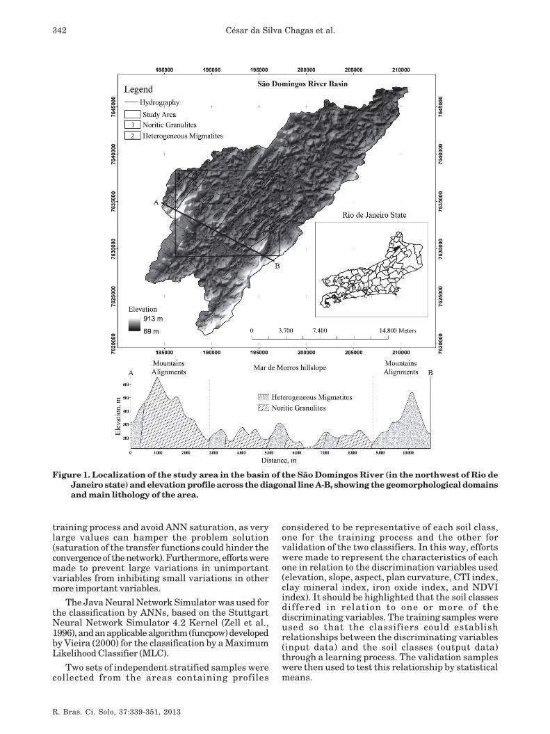
The contribution of the different variables in thediscrimination of soil class in Areas 1 and 2 are shownin table 2.

In general, the differentiation of the soil classesdetected by terrain attributes was much clearer thanby the Landsat 7 indices. Studies carried out by Doboset al. (2000, 2001) using terrain attributes and datafrom the Advanced Very High Resolution Radiometer(AVHRR) on the NOAA satellite for soil mappingshowed that terrain attributes alone were notsufficient for the discrimination of the soils in the areasstudied, while integrating this data with the AVHRRdata increased classification performance.

The best architecture for final data classificationwas selected based on the results of the Kappacoefficient and the overall accuracy, obtained usingthe validation samples (Figure 2).

In this evaluation, the highest values for the overallaccuracy and the Kappa coefficient for Area 1, obtainedusing the validation samples, were achieved usingnetwork architecture with only one input layercontaining 8 neurons (Kappa value of 0.908). TheKappa coefficient for Area 2 performed best when usinga network architecture with an input layer containingfive neurons (Kappa value of 0.893). An analysis ofthe Kappa significance matrix (Table 3) showedsignificant differences between these networks andthe others. These two architectures were thereforeselected for the final data classification.

On the other hand, using MLC in the classificationled to an overall accuracy of 84.4 % and a Kappacoefficient of 0.830 for Area 1, and an overall accuracy

of 72.3 % and a Kappa coefficient of 0.693 for Area 2.A comparison of the performances of the twoclassification types, based on an analysis of the Kappasignificance matrix, indicated significant differencesbetween these classifications for both areas (Table 4).

The results obtained in this evaluation are similarto those in other studies, in which the approach viaANNs generally led to better results than by the MLC,mainly in the classification of soil use and cover usingremote sensing data (Heermann & Khazenie, 1992;Bischof et al., 1992; Paola & Schowengerdt, 1995;McBratney et al., 2000).

Despite the significant differences between the twoclassifiers, with a better performance of the ANNclassification (Kappa values of 0.908 and 0.893 forAreas 1 and 2 respectively), it should be emphasizedthat this approach requires more time and morecomputational resources for the training process thanthe classic approach using the MLC. However, forYool (1998), ANNs have an advantage overconventional supervised classification methods suchas MLC, as these are inadequate and impractical forthe mapping of large areas.

According to Kanellopoulos & Wilkinson (1997),one aspect that has been neglected in the comparisonsbetween statistical classifiers and artificial neuralnetworks is the existence of significant differences inthe performance of these classifiers when classes areconsidered individually. The confusion matricesobtained for the tested classifications based on thevalidation set are presented in tables 5 and 6.

In the area characterized by noritic granulites(Area 1), the worst performance for ANN classificationoccurred for class PAe1 (62.0 %), with greatestconfusion with classes PVAe2, GXbe and LVAd. Inthe case of PVAe2 and GXbe, the confusion can beexplained by the extremely similar characteristics ofthe discriminating variables between these classes,mainly for slope, CTI index and the indices derivedfrom Landsat 7 (Table 2). For class LVAd, thedifferentiation was clearest with regard to elevation,slope and CTI index (Table 2); therefore, the confusionobserved must be attributed to an error in theclassifier. Accuracies exceeded 85 % for all other soilclasses (Table 5).

In the area characterized by HeterogeneousMigmatites (Area 2), the worst performance occurredfor class PVe5 (70.7 %), with greatest confusion withclass PVe6 (Table 5). These classes have very similarenvironmental characteristics and can bedifferentiated only by their aspect (Table 2). Accuraciesexceeded 95 % for all other soil classes (Table 5).

For the Maximum Likelihood classification (Table6), the performances in the classification of the areaof noritic granulites (Area 1) was poorest for theclasses PVAd (60 %) and PAe1 (56 %), versus 92.7and 62 % obtained using ANNs. The confusion of PVAdwas greater with PVe1, and since the average values


R. Bras. Ci. Solo, 37:339-351, 2013

ClasseElevation Slope Aspect Plan CTI Clay Iron

NDVI(m) (%) (degrees) curvature index minerals oxide

Area 1 - Noritic granulites

AR1 Average 634.24 83.73 145.54 0.09 5.01 126.31 80.06 151.10

S.D. 81.26 11.38 102.80 0.33 0.53 28.37 30.40 32.38

CXbe Average 426.23 29.97 182.65 0.04 5.69 148.73 66.12 173.27

S.D. 156.15 9.87 96.88 0.35 0.67 20.69 31.35 24.41

GXbe Average 128.19 1.68 179.38 0.00 9.98 124.88 117.06 135.58

S.D. 9.85 1.00 127.49 0.02 1.99 17.73 25.15 21.11

LVAd Average 221.60 8.52 180.63 0.05 6.61 118.61 119.08 120.03

S.D. 12.85 3.49 103.71 0.13 0.58 14.51 25.80 12.55

PAe1 Average 147.73 6.52 217.91 -0.01 8.22 124.16 114.20 132.42

S.D. 14.79 0.80 121.18 0.13 1.17 16.31 19.79 23.30

PVe1 Average 367.17 44.64 147.45 -0.40 6.89 137.53 92.64 152.08

S.D. 146.38 11.34 113.77 0.19 0.69 22.04 34.25 26.57

PVe2 Average 248.07 34.04 37.56 0.15 5.48 115.53 134.38 125.45

S.D. 72.85 10.97 18.74 0.13 0.35 17.25 32.87 14.93

PVe3 Average 231.80 36.63 308.82 0.16 5.64 116.29 108.80 120.09

S.D. 69.06 12.67 18.74 0.12 0.61 11.81 22.06 12.86

PVAe1 Average 237.01 36.35 239.59 0.12 5.48 124.04 88.73 122.08

S.D. 94.00 9.04 18.70 0.22 0.46 17.11 22.67 17.40

PVAe2 Average 135.75 11.07 138.85 -0.008 7.60 119.17 117.25 127.78

S.D. 22.41 1.80 81.60 0.13 1.00 17.49 22.63 18.59

PVAd Average 208.33 34.89 139.18 0.15 5.56 119.69 115.21 126.45

S.D. 65.99 8.52 22.63 0.19 0.45 16.33 25.70 19.75

RLe1 Average 717.55 57.59 208.11 0.14 5.21 156.26 43.63 179.93

S.D. 56.17 3.38 69.12 0.35 0.57 26.71 19.61 35.80

Area 2 - Heterogeneous migmatites

AR2 Average 487.79 82.40 191.04 0.18 4.90 122.57 62.32 112.57

S.D. 49.40 8.66 60.40 0.24 0.44 17.33 27.29 29.84

CXve Average 276.00 44.54 182.34 -0.10 6.47 127.85 97.51 137.03

S.D. 57.43 7.60 95.11 0.17 0.71 16.35 26.72 18.98

GXve Average 145.63 2.46 177.37 -0.001 9.71 120.86 112.20 132.46

S.D. 6.96 1.38 135.25 0.04 1.75 15.74 21.77 17.37

LVd Average 210.52 9.58 182.15 0.07 6.41 127.30 111.91 121.88

S.D. 11.46 3.94 96.85 0.13 0.43 12.55 21.61 12.17

PAe2 Average 158.65 5.53 220.38 0.01 8.20 118.44 109.37 133.88

S.D. 15.97 1.45 115.49 0.08 1.08 19.84 22.65 23.83

PVe4 Average 279.31 49.24 176.26 -0.08 6.25 127.27 93.85 133.03

S.D. 65.91 9.22 86.87 0.22 0.80 14.59 25.70 21.30

PVe5 Average 224.49 33.89 290.93 0.11 5.78 116.65 105.57 117.46

S.D. 52.73 9.33 73.25 0.18 0.60 10.61 24.38 12.69

PVe6 Average 237.63 32.41 128.41 0.13 5.61 118.13 113.22 123.98

S.D. 32.85 10.20 19.56 0.18 0.55 12.31 22.03 14.21

PVe7 Average 154.84 11.73 247.36 -0.02 7.48 123.28 107.54 133.32

S.D. 21.01 1.69 85.34 0.17 0.99 14.39 18.52 18.17

RLe2 Average 547.34 63.63 3.06 0.10 5.36 165. 62 46.33 167.39

S.D. 111.02 16.11 1.89 0.36 0.75 23.17 16.92 33.85

S.D.: standard deviation.

Table 2. Descriptive statistics for the discriminating variables between the soil classes


R. Bras. Ci. Solo, 37:339-351, 2013

346

of the discriminating variables of these classes arevery different (Table 2), it can be concluded that MLCwas less efficient than ANNs in the discrimination ofthese classes. The confusion of class PAe1 was greatestwith class PVAe2 (Table 6), in part related to thesimilarity of the discriminating variables betweenthese classes (Table 2). Therefore, the result of ANNsfor class PAe1 (62 %) suggests that MLC is lessefficient.

In the area characterized by HeterogeneousMigmatites (Area 2), the worst performances wereobtained for classes PVe6, PVe4 and GXve, withaccuracies of 44.7, 48.0 and 49.3 % respectively.Accuracies of 83.3, 92.7 and 97.3 % were obtainedusing ANNs for the same classes, which shows thatthe MLC was less efficient than ANNs in thediscrimination of these classes. For PVe6, the

Figure 2. Kappa coefficient obtained from the neural

networks tested.


Network R3(1) R5 R6 R7 R8 R9 R10 R15 R20 R25

Overall accuracy 86.6 813 86.4 86.9 91.6 89.2 88.6 88.0 89.7 78.9

Kappa 0.85 0.80 0.85 0.86 0.91 0.88 0.88 0.87 0.88 0.77

Variance(2) 0.077 0.100 0.078 0.075 0.051 0.063 0.067 0.070 0.061 0.110

R3 97.21

R5 4.28* 79.60

R6 0.08 4.20* 96.47

R7 0.41 4.69* 0.49 99.07

R8 4.86* 9.11* 4.93* 4.45* 127.15

R9 2.45* 6.74* 2.53* 2.04* 2.44* 111.12

R10 1.92 6.19* 1.99* 1.51 2.95* 0.53 107.02

R15 1.32 5.60* 1.40 0.91 3.55* 1.13 0.60 103.87

R20 2.30* 6.62* 2.38* 1.89 2.65* 0.18 0.35 0.96 112.67

R25 6.07* 1.79 5.98* 6.47* 10.88* 8.52* 7.97* 7.38* 8.41* 73.42


Network R3 R5 R6 R7 R8 R9 R10 R15 R20 R25

Overall accuracy 82.8 90.4 83.7 80.4 83.9 80.8 81.8 82.9 79.6 86.8

Kappa 0.809 0.893 0.819 0.782 0.822 0.787 0.798 0.811 0.774 0.853

Variance(2) 0.117 0.071 0.112 0.128 0.11 0.126 0.121 0.116 0.132 0.094

R3 74.79

R5 6.13* 105.98

R6 0.66 5.47* 77.39

R7 1.73 7.87* 2.39* 69.12

R8 0.86 5.28* 0.20 2.59* 78.38

R9 1.41 7.55* 2.07* 0.31 2.28* 70.11

R10 0.71 6.86* 1.38 1.01 1.58 0.70 72.55

R15 0.13 6.00* 0.53 1.86 0.73 1.54 0.84 75.30

R20 2.22* 8.35* 2.88* 0.50 3.09* 0.81 1.51 2.35* 67.37

R25 3.03* 3.11* 2.37* 4.77* 2.17* 4.45* 3.75* 2.90* 5.26* 87.98

Table 3. Significance matrix for the different architectures tested

* Significant difference of 95 %; (1) numbers correspond to the neurons in the hidden layer; (2) values multiplied by 1000.


R. Bras. Ci. Solo, 37:339-351, 2013

confusion with class PVe5 was greatest, as well as forGXve with PAe2 and PVe4 with PVe6 (Table 6). TheMLC performed well in discriminating the otherclasses, despite some confusion, with accuracy valuesexceeding 78.7 %.

Finally, a comparison between ANN and MLC showsa differentiated classification in Area 1, with ANNsperforming better for the classes AR1, GXbe, PAe1, PVe1,PVe2, PVe3, PVAd, PVAe2, and RLe1, while MLC wasonly better in the classification of CXbe and PVAe1. TheLVAd was classified equally by the two classifiers (Tables5 and 6). In Area 2, the ANN approach was better in theclassification of all classes except PVe5.

According to Landis & Koch (1977), the Kappacoefficient value obtained through the neural network


Class AR1 CXbe GXbe LVAd PAe1 PVe1 PVe2 PVe3 PVAe1 PVAe2 PVAd RLe1 Total User’s(1)

AR1 147 0 0 0 0 0 0 0 0 0 0 5 152 96.7

CXbe 0 135 0 0 0 1 1 0 0 0 0 2 139 97.1

GXbe 0 0 143 4 10 0 0 0 0 0 0 0 157 91.1

LVAd 0 0 0 131 8 0 2 0 0 3 4 0 148 88.5

PAe1 3 0 6 5 93 0 0 0 0 1 0 0 108 86.1

PVe1 0 0 0 2 0 145 1 1 0 0 0 1 150 96.7

PVe2 0 0 0 0 0 0 144 6 0 0 3 0 153 94.1

PVe3 0 0 0 0 0 2 0 140 3 1 0 0 146 95.9

PVAe1 0 1 0 0 0 1 0 3 146 0 4 0 155 94.2

PVAe2 0 0 1 6 39 0 2 0 0 143 0 0 191 74.9

PVAd 0 0 0 0 0 0 0 0 1 2 139 0 142 97.9

RLe1 0 14 0 0 0 1 0 0 0 0 0 142 157 90.4

Total 150 150 150 150 150 150 150 150 150 150 150 150 1800

Producer's(2)98.0 90.0 95.3 87.3 62.0 96.7 96.0 93.3 97.3 95.3 92.7 94.7

Overall accuracy = 91.6; Kappa = 0.908; Variance = 0.000051; Z calculated = 127.14; Z tabulated = 1.96


AR2 CXve GXve LVd PAe2 PVe4 PVe5 PVe6 PVe7 RLe2 Total User’s(1)

AR2 150 2 1 0 0 1 0 0 0 0 154 97.4

CXve 0 145 2 3 0 3 0 0 0 0 153 94.8

GXve 0 2 143 1 0 7 3 0 0 0 156 91.7

LVd 0 1 0 139 7 1 0 0 0 0 148 93.9

PAe2 0 0 3 1 106 3 0 7 0 0 120 88.3

PVe4 0 0 1 6 24 125 0 9 0 0 165 75.8

PVe5 0 0 0 0 3 0 128 2 0 1 134 95.5

PVe6 0 0 0 0 10 9 17 130 4 2 172 75.6

PVe7 0 0 0 0 0 0 0 0 146 3 149 98.0

RLe2 0 0 0 0 0 0 2 2 0 144 148 97.3

Total 150 150 150 150 150 150 150 150 150 150 1500

Producer's(2)100 95.3 97.3 86.7 96 92.7 70.7 83.3 85.3 96.7


Table 5. Confusion matrix obtained via ANN classification

(1) User accuracy of a pixel classified in the image actually representing the same category in the field (Vieira, 2000); (2) Produceraccuracy of a pixel being correctly classified in its class.

Classifier

Area 1 Area 2

Noritic Heterogeneous

granulites migmatites

ANN MLC ANN MLC

Overall accuracy 91.6 84.4 90.4 72.3

Kappa 0.908 0.830 0.893 0.693

Variance 0.000051 0.000086 0.000071 0.000162

ANN 127.145 105.98 -

MLC 6.66* 89.50 13.10* 54.45

Table 4. Significance matrix for the classifications

carried out in the two areas studied

* Significant difference of 95 %.


R. Bras. Ci. Solo, 37:339-351, 2013

348

approach indicates a very good to excellent performancefor this classifier (Kappa < 0.75) for both Area1 (0.908)and Area 2 (0.893). On the other hand, the MLCpresented a very good to excellent classification forArea 1 (0.830) and a moderate performance (0.4 <Kappa < 0.75) for Area 2.

Considering that some classes occupy small and/or very fragmented patches in the study area, somewere grouped together to facilitate understandingof the ANN- and MLC-based maps. The criteria forthis grouping was similarity in the characteristicsof the area of occurrence, as mentioned in the keyto Figure 3.

Although the results for the Kappa coefficientobtained from the validation samples were satisfactoryfor both classifiers, the resulting maps were different.


Class AR1 CXbe GXbe LVAd PAe1 PVe1 PVe2 PVe3 PVAe1 PVAe2 PVAd RLe1 Total User’s(1)

AR1 146 13 0 0 0 0 0 0 0 0 0 5 164 89

CXbe 0 137 0 0 0 0 0 0 0 0 0 21 158 86.7

GXbe 0 0 124 0 1 0 0 0 0 0 0 0 125 99.2

LVAd 0 0 0 131 3 0 9 0 0 0 0 0 143 91.6

PAe1 0 0 5 0 84 0 0 0 0 1 0 0 90 93.3

PVe1 0 0 0 4 0 141 3 21 1 8 33 0 211 66.8

PVe2 0 0 0 0 1 0 137 2 0 4 16 0 160 85.6

PVe3 0 0 0 0 0 0 0 123 2 1 0 0 126 97.6

PVAe1 0 0 0 0 0 5 0 4 147 0 9 0 165 89.1

PVAe2 0 0 21 14 61 0 0 0 0 136 2 0 234 58.1

PVAd 0 0 0 1 0 4 1 0 0 0 90 0 96 93.8

RLe1 4 0 0 0 0 0 0 0 0 0 0 124 128 96.9

Total 150 150 150 150 150 150 150 150 150 150 150 150 1800

Producer’s(2)97.3 91.3 82.7 87.3 56 94 91.3 82 98 90.7 60 82.7



AR2 CXve GXve LVd PAe2 PVe4 PVe5 PVe6 PVe7 RLe2 Total User’s(1)

AR2 150 0 0 0 0 1 0 0 0 24 175 85.7

CXve 0 120 0 0 0 0 0 4 0 26 150 80

GXve 0 0 74 0 0 0 0 0 0 0 74 100

LVd 0 0 0 103 0 0 6 3 17 0 129 79.8

PAe2 0 0 62 0 136 0 0 0 4 0 202 67.3

PVe4 0 0 0 0 0 72 3 4 0 0 79 91.1

PVe5 0 29 0 29 0 19 138 67 2 0 284 48.6

PVe6 0 0 0 0 0 53 0 66 1 0 120 55

PVe7 0 0 14 18 14 0 3 2 126 0 177 71.2

RLe2 0 1 0 0 0 5 0 4 0 100 110 90.9

Total 150 150 150 150 150 150 150 150 150 150 1500

Producer’s(2) 100 80 49.3 68.7 90.7 48 92 44.7 84 66.7 100


Table 6. Confusion matrix obtained using validation samples for classification using the maximum likelihood

algorithm

(1) User accuracy of a pixel classified in the image actually representing the same category in the field (Vieira, 2000); (2) Produceraccuracy of a pixel being correctly classified in its class.

The agreement between the ANN- and MLC-basedmaps was only 47.28 %. According to Kanellopoulos& Wilkinson (1997), this low agreement demonstratesthe differing nature of the mathematic models usedin the classifications and the way they structure thespace.

Figure 3 shows that both maps contain manyspatial details, reported by Zhu (2000). Using terrainattributes and geological properties as discriminatingenvironmental variables therefore showed the soil-landscape relationships in the area more clearly,resulting in spatially more detailed maps.

In the absence of a conventional soil map on anadequate scale ( < 50,000), reference points were usedto compare and evaluate the maps obtained usingANNs and MLC, according to Zhu (2000). In this


R. Bras. Ci. Solo, 37:339-351, 2013

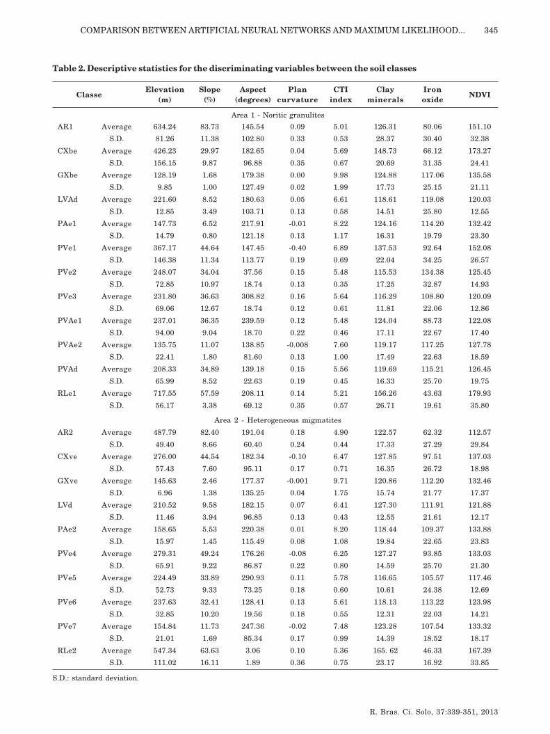
Figure 3. Maps obtained by the two classifiers.

comparison, the classification using ANNs correctlyinferred the soil classes at 93 locations (73.81 %) andMLC at 73 (57.94 %) (Table 6), which was comparableto results reported in other studies (Zhu, 2000; Zhuet al., 2001).

The matrix of Kappa significance (Table 7)indicated a significant difference between theclassifiers. Better results were obtained using ANNs(Kappa coefficient of 0.709), which were significantlydifferent from those obtained by MLC.

In the ANN classification, possible causes of thelow agreement with the reference points include therather complex geological nature of the area, whichin some situations impeded the correctdetermination of soil-landscape relationships; thequality of the geological map used; the lack ofinformation on the depth of lithic contact; andproblems related to the environmental correlationmodel used. Most misclassified observationsoccurred at the boundaries between the units of thegeological map. Problems related to the quality ofgeological maps used in environmental correlationstudies were also reported by Thomas et al. (1999)and McKenzie & Ryan (1999).

McKenzie & Austin (1993) found that the presenceof an impediment layer at low depths is a strongpredictor of soil properties and the presence ofgeological structures such as dikes can control thesoil distribution pattern. Dikes of basic material arecommon in the area studied, but are not shown onthe geological map (DRM-RJ, 1980).

On the other hand, McKenzie & Ryan (1999)emphasized that there are circumstances in whichsoil variation occurs without any direct relation toeasily observable environmental variables (lack of areliable predictor) and in these cases, detailed samplingis inevitable and some form of interpolation isnecessary to generate a spatial prediction.

In the case of MLC-based classifications, the lowagreement with the reference points was mostly dueto the inefficiency of the classifier.

The main lack of agreement between ANN- andMLC-based classifications can be verified in the flatterareas of the landscape (flat and gently undulatingtopography), classified by ANNs as belonging to theHaplic Gleysol class (GXbe and GXve for Areas 1 and2 respectively) and by MLC as belonging to classesPVAe2 and PVe7 (for Areas 1 and 2 respectively),which occurs in undulating topography. In this case,the ANN-based classification was more accurate whileMLC was less effective in adequately discriminatingareas with very similar slope values.

Conversely, by the ANN-based classification theclass LVd (top-left corner of the image) was incorrectlyidentified in areas that should have been classified asbelonging to class PVe7. In spite of the similar slopevalues of these classes, they occupy different positionson the landscape, with class LVd in even areas athigh elevations and class PVe7 in the lower third ofslopes close to wetlands. This result demonstrates aninefficiency in the ANN-based classification that wasnot observed for the MLC-based classification.


R. Bras. Ci. Solo, 37:339-351, 2013

350

Table 7. Confusion matrix between the maps

obtained using ANN and MLC considering

reference points

Classification ANNs MLC

Total number of points 126 126

Correctly classified points 93 73

Overall accuracy 73.81 57.94

Kappa 0.709 0.534

Variance 0.001826 0.002236

Neural network 16.59

Maximum likelihood 2.75* 11.29

* Significant difference of 95 %.

CONCLUSIONS

1. The Artificial Neutral Network classifierresulted in a higher accuracy for general classificationwhen validation samples were used, producingsignificantly better statistical results than theMaximum Likelihood Classifier.

2. A comparison of reference points showed thatthe ANN-based was more accurate than the MLC-based map, which was significantly different. Themain cause of data classification errors of theclassifiers may be related to the geologicalheterogeneity of the area, the depth of lithic contactand problems associated with the environmentalcorrelation model used, including the discriminatingvariables selected.

3. The use of terrain attributes and remote sensingdata with spatial resolution compatible with theobjectives of the study, together with a neural networkapproach, can help accelerate, extend and cheapensoil mapping in Brazil, due to the availability of lower-cost digital satellite images and the ease at whichterrain attributes can be obtained.

LITERATURE CITED

ATKINSON, P.M. & TATNALL, A.R.L. Neural networks inremote sensing. Inter. J. Remote Sens., 18:699-709, 1997.

BEHRENS, T.; FOSTER, H.; SCHOLTEN, T.; STEINRUCKEN,U.; SPIES, E.D. & GOLDSCHMITT, M. Digital soil mappingusing artificial neural networks. J. Plant Nutr. Soil Sci.,168:21-33, 2005.

BENEDIKTSSON, J.A. & SVEINSSON, J.R. Featureextraction for multisource data classification with artificialneural networks. Inter. J. Remote Sens., 18:727-740,1997.

BISCHOF, H.; SCHNEIDER, W. & PINZ, A.J. Multispectralclassification of Landsat-images using neural networks.IEEE Trans. Geosci. Remote Sens., 30:482-490, 1992.

BORUVKA, L. & PENIZEK, V. A test of an artificial neuralnetwork allocation procedure using the Czech soilsurvey of agricultural land data. In: LAGACHERIE, P.;McBRATNEY, A. B. & VOLTZ, M., eds. Digital soilmapping: An introductory perspective. Amsterdam,Elsevier, 2007. p.415-424. (Developments in SoilScience, 31)

BRUS, D.J. & HEUVELINK, G.B.M. Optimization of samplepatterns for universal kriging of environmental variables.Geoderma, 138:86-95, 2007.

CHAGAS, C.S.; FERNANDES FILHO, E.I.; VIEIRA, C.A.O.;SCHAEFER, C.E.G.R. & CARVALHO JÚNIOR, W.Atributos topográficos e dados do Landsat7 nomapeamento digital de solos com uso de redes neurais.Pesq. Agropec. Bras., 45:497-507, 2010.

CHAGAS, C.S.; CARVALHO JÚNIOR, W. & BHERING, S.B.Integração de dados do Quickbird e atributos do terrenono mapeamento digital de solos por redes neuraisartificiais. R. Bras. Ci. Solo, 35:693-704, 2011.

CONGALTON, R.G. & GREEN, K. Assessing the accuracy ofremotely sensed data: Principles and practices. New York,Lewis Publishers, 1999. 160p.

CONGALTON, R.G. & MEAD, R.A. A review of discretemultivariate analysis techniques used in assessing theaccuracy of remotely sensed data from error matrices.IEEE Trans. Geosci. Remote Sens., 24:169-174, 1986.

DEPARTAMENTO DE RECURSOS MINERAIS - DRM-RJ.Projeto Carta Geológica do Estado do Rio de Janeiro naEscala 1:50.000. Folhas: Miracema e São João do Paraíso.1980.

DOBOS, E.; MICHELI, E.; BAUMGARDNER, M.F.; BIEHL, L.& HELT, T. Use of combined digital elevation model andsatellite data for regional soil mapping. Geoderma, 97:367-391, 2000.

DOBOS, E.; MONTANARELLA, L.; NÈGRE, T. & MICHELI,E. A regional scale soil mapping approach using integratedAVHRR and DEM data. Inter. J. Appl. Earth Obs. Geoinf.,3:30-42, 2001.

ELNAGGAR, A.A. & NOLLER, J.S. Application of remotesensing data and decision-tree analysis to mapping ofsalt-affected soils over large areas. Remote Sens., 2:151-165, 2010.

EMPRESA BRASILEIRA DE PESQUISA AGROPECUÁRIA -EMBRAPA. Centro Nacional de Pesquisa de Solos.Levantamento de reconhecimento de baixaintensidade dos solos do Estado do Rio de Janeiro. Riode Janeiro, 2003. 242p. (Boletim de Pesquisa eDesenvolvimento, 32)

EMPRESA BRASILEIRA DE PESQUISA AGROPECUÁRIA -EMBRAPA. Centro Nacional de Pesquisa de Solos.Procedimentos normativos de levantamentos pedológicos.Brasília, 1995. 101p.

EMPRESA BRASILEIRA DE PESQUISA AGROPECUÁRIA -EMBRAPA. Centro Nacional de Pesquisa de Solos.Sistema brasileiro de classificação de solos. 2.ed. Rio deJaneiro, 2006. 306p.


R. Bras. Ci. Solo, 37:339-351, 2013

ENVIRONMENTAL SYSTEMS RESEARCH INSTITUTE -ESRI. ArcGIS Desktop. Redlands, 2010. v.10.

GALLANT, J.C. & WILSON, J.P. Primary topographicattributes. In: WILSON, J.P. & GALLANT, J.C., eds.Terrain analysis: Principles and applications. New York,John Wiley & Sons, 2000. p.51-85.

GIASSON, E.; SARMENTO, E.C.; WEBER, E.; FLORES,C.A. & HASENACK, H. Decision trees for digital soilmapping on subtropical basaltic steeplands. Sci. Agric.,68:167-174, 2011.

HEERMANN, P.D. & KHAZENIE, N. Classification ofmultispectral remote sensing data using a back-propagation neural network. IEEE Trans. Geosci.Remote Sens., 30:81-88, 1992.

HENGL, T.; TOOMANIAN, N.; REUTER, H.I. &MALAKOUTI, M.J. Methods to interpolate soilcategorical variables from profile observations: Lessonsfrom Iran. Geoderma, 140:417-427, 2007.

JENNY, H. Factors of soil formation; a system ofquantitative pedology. New York, McGraw-Hill, 1941.281p.

KANELLOPOULOS, I. & WILKINSON, G.G. Strategiesand best practice for neural network imageclassification. Inter. J. Remote Sens., 18:711-725, 1997.

LANDIS, J.R. & KOCH, G.G. The measurement of observeragreement for categorical data. Biometrics, 33:159-174,1977.

McBRATNEY, A.B.; ODEH, I.O.A.; BISHOP, T.F.A.;DUNBAR, M.S. & SHATAR, T.M. An overview ofpedometrics techniques for use in soil survey.Geoderma, 97:293-327, 2000.

McBRATNEY, A.B.; SANTOS, M.L.M. & MINASNY, B. Ondigital soil mapping. Geoderma, 117:3-52, 2003.

McKENZIE, N.J. & AUSTIN, M.P. A quantitative Australianapproach to medium and small scale surveys based onsoil stratigraphy and environmental correlation.Geoderma, 57:329-355, 1993.

McKENZIE, N.J. & RYAN, P.J. Spatial prediction of soilproperties using environmental correlation. Geoderma,89:67-94, 1999.

NARASIMHA RAO, P.V.; VENKATARATNAM, L.;KRISHNA RAO, P.V.; RAMANA, K.V. & SINGARAO,M.N. Relation between root zone soil moisture andnormalized difference vegetation index of vegetatedfields. Inter. J. Remote Sens., 14:441-449, 1993.

PAOLA, J.D. & SCHOWENGERDT, R.A. A detailed comparisonof backpropagation neural network and maximum-likelihood classifiers for urban land use classification. IEEETrans. Geosci. Remote Sens., 33:981-996, 1995.

SABINS JUNIOR, F.F. Remote sensing: Principles andinterpretation. 3.ed. New York, W. H. Freeman andCompany, 1997. 432p.

THOMAS, A.L.; KING, D.; DAMBRINE, E. & COUTURIER, A.Predicting soil classes with parameters derived from reliefand geologic materials in a sandstone region of the Vosgesmountains (Northeastern France). Geoderma, 90:291-305, 1999.

TSO, B. & MATHER, P.M. Classification methods for remotelysensed data. 2.ed. Boca Raton, CRC, 2009. 356p.

WEINDORF, D.C. & ZHU, Y. Spatial variability of soilproperties at Capulin Volcano, New Mexico, USA:implications for sampling strategy. Pedosphere, 20:185-197, 2010.

WIEGAND, C.L.; RICHARDSON, A.J.; ESCOBAR, D.E. &GERBERMANN, A.H. Vegetation indices in cropassessments. Remote Sens. Environ., 35:105-119, 1991.

YANG, W.; YANG, L. & MERCHANT, J.W. An assessment ofAVHRR/NDVI-ecoclimatological relations in Nebraska,USA. Inter. J. Remote Sens., 18:2161-2180, 1997.

YOOL, S.R. Land cover classification in rugged areas usingsimulated moderate-resolution remote sensor data andan artificial neural network. Inter. J. Remote Sens., 19:85-96, 1998.

ZELL, A.; MAMIER, G.; VOGT, M.; MACHE, N.; HUBNER, R.;DORING, S.; HERRMANN, K.; SOYEZ, T.; SCHMALZL,M.; SOMMER, T.; HATZIGEORGIOU, A.; POSSELT, D.;SCHREINER, T.; KETT, B.; CLEMENTE, G.; WIELAND,J. & GATTER, J. Stuttgart neural network simulator:User manual. Version 4.2. Stuttgart, University ofStuttgart, 1996. 338p.

TEN CATEN, A.; DALMOLIN, R.S.D.; PEDRON, F.A. &MENDONÇA-SANTOS, M.L. Regressões logísticasmúltiplas: Fatores que influenciam sua aplicação napredição de classes de solos. R. Bras. Ci. Solo, 35:53-62,2011.

ZHU, A.X. Mapping soil landscape as spatial continua: The neuralnetwork approach. Water Res. Res., 36:663-677, 2000.

ZHU, A.X.; HUDSON, B.; BURT, J.; LUBICH, K. &SIMONSON, D. Soil mapping using GIS, expertknowledge, and fuzzy logic. Soil Sci. Soc. Am. J., 65:1463-1472, 2001.

COMPARISON BETWEEN ARTIFICIAL NEURAL NETWORKS … · COMPARISON BETWEEN ARTIFICIAL NEURAL NETWORKS...

Documents

Transcript of COMPARISON BETWEEN ARTIFICIAL NEURAL NETWORKS … · COMPARISON BETWEEN ARTIFICIAL NEURAL NETWORKS...