Comparing Open and Sealed Bid Auctions: Theory and Evidence ...
55
Comparing Open and Sealed Bid Auctions: Theory and Evidence from Timber Auctions ∗ Susan Athey, Jonathan Levin and Enrique Seira † March 2004 Preliminary and Incomplete Draft Abstract We study entry and bidding patterns in sealed bid and open auctions with heterogeneous bidders. We extend the theory of private value auctions with heterogeneous bidders to allow for endogenous participation. The theory pre- dicts that sealed bid auctions should attract more small bidders and fewer large bidders relative to open auctions, and also tend to generate more revenue. We examine these predictions using data from U.S. Forest Service timber auctions. We find that sealed bid auctions do attract more small bidders and raise more revenue than open auctions when the pool of potential entrants is heterogenous, but not when the pool of entrants is homogenous. The latter finding is con- sistent with the Revenue Equivalence Theorem of the standard auction model, while the former is generally consistent with our extension of the theory. ∗ We thank Guido Imbens, Phil Haile and Richard Levin for their advice and Jerry Hausman for helpful suggestions at the early stages of this project. Athey and Levin acknowledge the support of the National Science Foundation. † Athey: Stanford University and NBER, [email protected]; Levin: Stanford University, [email protected]; Seira: Stanford University, [email protected].
Transcript of Comparing Open and Sealed Bid Auctions: Theory and Evidence ...

Comparing Open and Sealed Bid Auctions:
Theory and Evidence from Timber Auctions∗
Susan Athey, Jonathan Levin and Enrique Seira†
March 2004
Preliminary and Incomplete Draft
Abstract
We study entry and bidding patterns in sealed bid and open auctions with
heterogeneous bidders. We extend the theory of private value auctions with
heterogeneous bidders to allow for endogenous participation. The theory pre-
dicts that sealed bid auctions should attract more small bidders and fewer large
bidders relative to open auctions, and also tend to generate more revenue. We
examine these predictions using data from U.S. Forest Service timber auctions.
We find that sealed bid auctions do attract more small bidders and raise more
revenue than open auctions when the pool of potential entrants is heterogenous,
but not when the pool of entrants is homogenous. The latter finding is con-
sistent with the Revenue Equivalence Theorem of the standard auction model,
while the former is generally consistent with our extension of the theory.
∗We thank Guido Imbens, Phil Haile and Richard Levin for their advice and Jerry Hausman forhelpful suggestions at the early stages of this project. Athey and Levin acknowledge the support ofthe National Science Foundation.
†Athey: Stanford University and NBER, [email protected]; Levin: Stanford University,[email protected]; Seira: Stanford University, [email protected].

1. Introduction
Auction design has become increasingly important in many markets. A central,
and frequently debated, design issue concerns the relative performance of open and
sealed bid auctions. This choice comes up in structuring sales of natural resources,
art, antiques and real estate, in auctioning construction and procurement contracts, in
asset liquidation sales, and in designing ongoing bidding markets such as restructured
electricity markets.
Economic theory provides on the one hand very little and on the other hand per-
haps too much guidance on the merits of open and sealed bid auctions. The seminal
result in auction theory, Vickrey’s (1961) Revenue Equivalence Theorem, states that
under certain conditions, the two formats have essentially equivalent equilibrium out-
comes. Specifically, if bidders are risk-neutral and have independent and identically
distributed values, the two auctions yield the same winner, the same expected revenue,
and even the same bidder participation. In practice, however, these assumptions of-
ten seem too strong. Further work points out that as they are relaxed, auction choice
becomes relevant, with the comparison between open and sealed bidding depending
on both the details of the market (e.g. whether the key feature is bidder heterogene-
ity, collusion, common rather than private values, risk-aversion, transaction costs and
so on) and the designer’s objective (e.g. revenue maximization or efficiency).
There has been less progress in providing empirical evidence on the performance
of alternative auction designs. A difficulty is that many real-world auction markets
tend to operate under a given set of rules rather than systematically experimenting
with alternative designs. In this paper, we combine theory and empirical analysis
to study the use of open and sealed bid auctions to sell timber from the national
forests. The U.S. Forest Service timber program provides an excellent test case in
market design as it has historically used both open and sealed auctions, at times even
randomizing the choice. The timber sale program is also economically interesting in
its own right. Timber logging and milling is a $100 billion a year industry in the
U.S.,1 and about 30% of timberland is publicly owned. During the time period we
study, the federal government sold about a billion dollars of timber a year.
1This number is from the U.S. Census and combines forestry and logging, sawmills, and pulp andpaperboard mills (NAICS categories 113, 3221 and 321113).
1

A long-standing debate surrounds the design of federal timber auctions. An early
study by Mead (1967) argued that open auctions generated less revenue. In 1976,
Congress mandated the use of sealed bidding. The law, however, left a loophole
that allowed forest managers to use open auctions if they could justify the choice.
As a result, sale method has varied geographically. In the Pacific Northwest, the
largest Forest Service region, open auctions have predominated apart from a short
period following the 1976 law. We focus instead on the neighboring Northern region
comprised of Idaho and Montana, and provide additional evidence from California
sales.
We start by developing a theoretical model that incorporates two key features of
the timber market into the standard independent private value auction model. First,
we allow bidders to have heterogeneous value distributions. There is substantial vari-
ation among participants in Forest Service auctions, where the bidders range from
large vertically integrated forest products conglomerates to individually-owned log-
ging companies. To capture this heterogeneity, we assume as in Maskin and Riley
(2000) that stronger bidders have value distributions that stochastically dominate
those of weaker bidders. Our second departure from the standard model is to en-
dogenize participation by making it costly to acquire information and bid in the
auction. Explicitly modeling participation makes the model more realistic, and more
importantly gives rise to new testable hypotheses about entry patterns.2
The theory generates predictions about how entry, allocation and revenue will
vary by auction format. When bidders are homogeneous, auction format will have
no systematic effect on any of these outcome variables. With heterogeneous bidders,
however, sealed bidding promotes entry by bidders who are relatively weak from an
ex ante standpoint and discourages entry by bidders who are relatively strong. The
allocation in a sealed auction also shifts toward weaker bidders, both because of entry
and because in the sealed bid equilibrium, weaker firms submit bids with a smaller
profit margin than stronger firms. Finally we conjecture that prices will tend to be
higher with sealed bidding, though we are unable to provide a general theorem to
support this claim.
2Several papers study entry decisions in auctions with symmetric bidders, but discussion of entrywith asymmetric bidders has been limited to examples. Milgrom (2004, chapter 6) provides aninsightful overview.
2
The argument behind these results runs as follows. With an open auction, the
entrant with the highest value always wins. This makes weak bidders hesitant to
spend money to participate if strong bidders are also likely to be present. In contrast,
in a sealed bid auction, strong bidders have a relatively large incentive to shade their
bids below their true valuations, so a weaker bidder can win despite not having the
highest valuation. This handicapping effect promotes the entry of weaker bidders
and discourages the entry of strong bidders.3 The expected winning bid can also
rise because weak bidders provide more competition for strong bidders when bids are
sealed.
We use the competitive bidding theory to frame our empirical investigation of
timber auctions. Our analysis focuses on sales that occurred between 1982 and 1990
in two large neighboring forests in Idaho and Montana. We also provide additional
evidence from sales in California forests. All of these forests use a mixture of open
and sealed bid auctions. We address the issue of bidder heterogeneity by classifying
the bidders into two groups: mills that have manufacturing capacity and loggers that
do not. We provide a variety of evidence that mills tend to have higher values for
a given contract than logging companies, which have to re-sell the timber if they
win the contract. Using manufacturing capability as a proxy for bidder strength, we
investigate the model’s implications for entry, revenue and allocation.
Our first finding is that, conditional on sale characteristics, sealed bid auctions
induce significantly more loggers to participate. The entry of mills appears not to vary
much across auction formats. So total participation is higher in sealed bid auctions
and a greater fraction of the participants are logging firms. The higher entry suggests
that sealed bid auctions may generate higher prices on average. We find that this is
indeed the case. In the Idaho and Montana forests, winning bids are 10-20% higher in
the sealed bid auctions. In the California forests, the difference is around 8-9%. We
3The first half of this argument figured prominently in the design of the British 3G spectrumauction. In the initial design phase of that auction, the number of licenses was to be just equal tothe number of incumbent firms, whose entry was assured. Concerned that there would be little denovo entry to raise prices in an open auction, the lead designer Paul Klemperer proposed an “Anglo-Dutch” design that would have added a sealed bid component to the auction. Ultimately concernsabout entry were alleviated by adding another license and it was possible to run a successful openauction. Interestingly, the Netherlands faced the same problem in their 3G auction design. Theyended up running an open auction despite having a number of licences just equal to the number ofincumbents. This resulted in minimal entry and very low prices.
3
show that the revenue advantage of the sealed bid auctions can be attributed partly
to the increase in participation, and partly to the fact that sealed auctions appear
to generate higher revenue for any given set of bidders. Lastly, we consider how the
identity of the winning bidder varies by auction format. We find that in Idaho and
Montana, loggers are in fact no more likely to win the sealed bid auctions, which is
surprising given the patterns of entry we observe. California differs in this regard;
loggers appear somewhat more likely to win sealed bid sales.
For the purposes of comparison, we then look at a second set of small business
set-aside sales in the Idaho and Montana forests.4 In these sales, participation is
restricted to firms with less than 500 employees. Because of this, the set of potential
participants is arguably far more homogeneous. Indeed the participants are primarily
logging companies; there is very little entry by mills. We find that in these set-aside
sales, the differences in entry and sale prices between open and sealed bid auctions are
small and we cannot reject the hypothesis of zero auction format effect. This is the
result predicted by the Revenue Equivalence Theorem, which applies when bidders
are perfectly homogeneous.
Overall, we interpret these findings as being reasonably consistent with the com-
petitive model, though not perfectly so. This leads us to consider whether factors
not captured by our relatively simple model might explain the discrepancies. Possi-
bilities include differences in transactions costs, the possibility of tacit collusion, or
the presence of unobserved heterogeneity between the sales that be confounding our
interpretation of the empirical results. Of these, a degree of tacit cooperation among
the larger firms seem potentially able to explain our findings.
In the final part of the paper, we ask whether the competitive model can plau-
sibly account for the observed quantitative differences in our data. We estimate the
distribution of bids in the Idaho and Montana sealed bid auctions and use the tech-
niques pioneered by Guerre, Perrigne and Vuong (2001) to recover the pseudo-values
that rationalize these bids. We then ask whether the value distributions for mills and
loggers inferred from the sealed bid auctions can explain the prices we observe in the
open auctions. Using the inferred value distributions, we simulate open auctions and
compare the resulting prices to the open auction prices in the data. We find that
the simulated prices are higher than the observed prices. One interpretation is that
4There were few small business sales in the California forests, so we focus on Idaho and Montana.
4

bidding behavior is less competitive at the open auctions.
Our paper is the first empirical study we are aware of that focuses on differential
entry and the importance of bidder heterogeneity across auction formats. Several prior
studies have looked directly at revenue differences between open and sealed bid timber
auctions. Johnson (1979) and Hansen (1986) study sales in the Pacific Northwest
following the passage of the 1976 sealed bidding mandate. They reach conflicting
conclusions: Johnson finds that the sealed bid auctions raised more revenue, while
Hansen argues that the differences are insignificant after accurately accounting for
sale characteristics. The episode is not, however, an ideal testing ground. As Hansen
points out, the choice of auction format during this period was sensitive to lobbying,
creating a potentially severe endogeneity problem that is hard to address empirically.
Moreover, one might naturally be skeptical of testing equilibrium predictions in an
unexpected and transient episode.
Subsequent to these studies, Shuster and Nicolluci (1993) and Stone and Rideout
(1997) looked, respectively, at sales in Idaho and Montana and in Colorado. Both
papers find higher revenue from sealed bid auctions. A nice feature of Shuster and
Nicolluci’s paper is that they exploit the often-random assignment of auction format
in some of the Idaho and Montana forests. Though we address a broader set of
questions and from a somewhat different perspective, we have drawn on their work
to select our data sample.
Apart from these studies, there is also a body of research considering open and
sealed bid auctions in experimental, or quasi-experimental settings. Kagel (1995) is
a standard reference, while Lucking-Reilly (2000) reports results from a clever series
of internet field experiments. This research emphasizes that auction theory results
even more basic than the revenue equivalence theorem – such as the equivalence
of ascending bid and second-price sealed bid auctions – often fail in experimental
settings.
2. Comparing Auctions: Theory
This section develops the model of competitive bidding that we use to frame our
empirical analysis. We extend the heterogeneous private values model of Maskin and
5

Riley (2000) to allow for endogenous participation decisions. We characterize equi-
librium behavior and derive empirically testable predictions comparing equilibrium
entry and bidding in sealed bid and open auctions.
A. The Model
We consider an auction for a single tract of timber. Prior to the sale, the seller
announces a reserve price r and the auction format: open ascending or first price
sealed bid. There are n potential risk-neutral bidders. Each bidder i has a private
cost ki of gathering information and entering the auction. By paying the entry cost,
bidder i learns his value for the tract, vi, and may bid for the tract.
Entry costs and values are assumed to be independent across bidders. We model
entry costs as draws from a distribution H (·) with support [0, k], and each bidderi’s value as a draw from a distribution Fi. The bidders are heterogeneous if the
distributions F1, ..., Fn are not identical. In this case, we assume that Fi stochastically
dominates Fi+1, so bidders are ordered from strongest to weakest. We will also assume
that bidders are serious in the sense that there is a lower bound on the probability
that each bidder decides to acquire information. To this end, we assume there is a
positive chance of having a zero cost of gathering information, so H(0) = ϕ > 0.
Assumption For all bidders i = 1, ..., n,
(i) Fi has a continuous density fi on [v, vi], where v < r.
(ii) For all v ≥ r, Fi(v) ≤ Fi+1(v).
(iii) For all v ≥ r, fi(v)Fi(v)− fi+1(v)
Fi+1(v)≥ fi(v)−fi+1(v)
Fi(v)Fi+1(v)(1− 1/ϕ).
Assumption (i) implies that the reserve price is at least occasionally binding. This is
useful to establish equilibrium existence, but is probably not necessary. Assumption
(ii) states that bidder i’s values are higher than i + 1’s in the sense of first-order
stochastic dominance. Assumption (iii) is closely related to Maskin and Riley’s (2000)
assumption that Fi has a higher reverse hazard rate than Fi+1 (they coincide if ϕ = 1),
and plays the same role – helping to ensure that in equilibrium, i’s bid distribution
dominates i+ 1’s in the sense of having a higher reverse hazard rate.5
5Assumption (iii) is a stronger assumption than necessary for our key result that smaller bidders
6

We adopt a standard model of the bidding process. In an open auction, the price
rises from the reserve price and the auction terminates when all but one participating
bidder has dropped out. With sealed bidding, participating bidders independently
choose a bid to submit; the highest bidder wins and pays his bid. In the sealed bid
auction, we assume that bidder i submits his bid without knowledge of the exact set
of participants, but rather only knows the potential entrants. This seems to be the
natural way to model timber auctions, where bidders do not have to submit advance
notice that they intend to bid. Our main results, however, would also hold in a model
where bidders learn the identities of the other participants before deciding how much
to bid. We discuss this, and other specifications of the entry process, below.
A strategy for bidder i consists of a bidding strategy and an entry strategy. A
bidding strategy bi(·) specifies i’s bid (or drop-out point in the case of an open auction)as a function of his value. An entry strategy specifies whether he should enter as a
function of his entry cost. An optimal entry strategy will always be a threshold rule,
with bidder i entering if and only if his cost lies below some threshold Ki.
An entry equilibrium is a set of bidding strategies b1(·), ..., bn(·) and entry costthresholdsK1, ...,Kn with the property that: (i) each bidder’s bid strategy maximizes
his profits conditional on entering; and (ii) each bidder finds it optimal to enter if
and only if his entry cost lies below his cost threshold. As is often the case with entry
models, there may be many equilibria. We focus on equilibria that are monotone
in the sense that strong bidders enter more often, i.e. where K1 ≥ ... ≥ Kn. Even
with this restriction, equilibrium need not be unique; for this reason, our results will
compare sets of equilibria across auction methods.
B. Sealed Bid Auctions
We solve for the equilibrium of the sealed bid auction in two steps. We first
characterize optimal bidding under the assumption that entry behavior is given by an
arbitrary set of monotone entry cost thresholds K1 ≥ ... ≥ Kn. We then characterize
the equilibrium entry strategies. Here and in the succeeding sections, we focus on the
main ideas, deferring detailed proofs to the Appendix.
prefer sealed auctions, but we haven’t found a weaker alternative that is simple to state in terms ofexogenous parameters. In slight variations on our model, Maskin and Riley’s hazard rate orderingcondition suffices for our result. Future drafts will include more discussion of these points.
7

Let K = (K1, ..., Kn) denote a set of monotone entry cost thresholds. Suppose
that bidder i decides to participate and learns he has value vi ≥ r. We can write his
expected profit as:
Πsi (v;K) := max
b≥r(vi − b)
Yj 6=i
Gj(b), (1)
where Gj(b) is the probability that a bid of b will beat bidder j. From i’s perspective,
both j’s participation and j’s bid conditional on entering are random variables. If j
has an entry thresholdKj and a continuous bid strategy bj(·) that is strictly increasingfor values above the reserve price (as will be the case in equilibrium), then for b ≥ r :
Gj(b) := 1−H(Kj) +H(Kj)F (b−1j (b)). (2)
The first order condition for i’s bidding problem is:
1
vi − bi=Xj 6=i
gj(bi)
Gj(bi). (3)
Given the entry cost thresholds K1, ..., Kn, the system of equations given by (2)
and (3), together with the boundary condition that bi(r) = r for all i, uniquely
characterizes a set of optimal bidding strategies b1(·), ..., bn(·). In particular, given anequilibrium set of entry cost thresholds, the equilibrium bidding strategies will solve
(2) and (3), where (2) is evaluated at the appropriate cost thresholds K1, ...,Kn.
To identify the equilibrium entry thresholds, observe that a bidder should enter
whenever his expected profits exceed his entry cost. Bidder i’s expected profit from
entry, given a set of entry thresholds and the induced optimal bidding strategies, is:
Πsi (K) =
ZΠsi (vi;K)dFi(vi).
So the equilibrium entry cost thresholds satisfy:
Ksi = max{Πs
i (Ks), k}. (4)
Proposition 1 A monotone entry equilibrium, characterized by equations (1)—(4),
exists in the sealed bid auction. In any such equilibrium: (i) strong bidders submit
8

higher bids: G1(b) ≤ ... ≤ Gn(b) for all b ≥ r, despite the fact that (ii) strong bidders
shade their bids more than weaker bidders: b1(v) ≤ ... ≤ bn(v) for all v.6
The first part of the Proposition states that in equilibrium strong bidders will tend
to submit higher bids than weak bidders. From an empirical standpoint, this will
provide a straightforward test of whether we have accurately classified heterogeneous
bidders in terms of their strength. Note that the Proposition does not state that strong
bidders necessarily make higher bids conditional on entry (though they may) but
rather that they are stronger competitors having factored in their higher probability
of entry. This is what matters to opponents.
The second part of the Proposition is important for our comparative predictions.
It states that in a sealed bid equilibrium, strong bidders shade their bids more weak
bidders, a natural result given that strong bidders face weaker competition. The
consequence is that a weak entrant may win despite not having the highest value.
We will show that this provides an extra incentive for weak bidders to participate,
raising their equilibrium probability of entry relative to an open format.
C. Open Auctions
Next we consider equilibrium in the open auction. Again we proceed by character-
izing optimal bidding behavior given a set of entry cost thresholds K = (K1, ...,Kn)
and then identifying the equilibrium entry strategies.
Optimal bidding in an open auction is simpler than in the sealed bid case because
for an entering bidder, it is a dominant strategy to continue bidding until the price
reaches his valuation. This is true regardless of the number of entering bidders.
Therefore bi(v) = v for all bidders i and all values v ≥ r irrespective of the entry
strategies.
As above, it is useful to write bidder i’s expected profits from entering as a function
of his value vi and the entry strategies. Let
Gj(b) = 1−Hj(Kj) +Hj(Kj)Fj(b)
6Results (i) and (ii) are shown for the case of fixed participation in Maskin and Riley (1999) andLi and Riley (1999). This proposition extends their results to the case of endogenous participation.
9
denote the probability that a bid of b will beat bidder j. Then bidder i’s expected
profit, conditional on entering and having a value vi ≥ r is:
Πoi (vi;K) := max
b≥r(vi − E[max{b−i, r}|b−i ≤ b])
Yj 6=i
Gj(b), (5)
where b−i denotes the set of competing bids, and i’s optimal strategy, of course, is to
bid his value vi.
We identify the equilibrium entry cost thresholds just as in the sealed bid case.
We write i’s expected profits as a function of the entry cost thresholds:
Πoi (K) =
ZΠoi (vi;K)dFi(vi),
and note that in equilibrium, each bidder should enter whenever his expected profit
from entry exceeds his cost of entry. So the equilibrium entry cost thresholds satisfy:
Koi = max{Πo
i (Ko), k}. (6)
Proposition 2 A monotone entry equilibrium exists in the open bid auction. In any
such equilibrium, (i) strong bidders submit higher bids: G1(b) ≤ ... ≤ Gn(b) for all
b ≥ r, and (ii) all entrants bid their true value, bi(v) = v for all i, v.
In equilibrium, strong bidders enter more often and bid more conditional on en-
tering. The latter point follows because entering bidders stay in the auction until the
price reaches their valuation. A consequence is that, given a set of entrants, the open
auction is efficient. The entrant with the highest value always wins. As we will see,
this tends to discourage the entry of weak bidders relative to the sealed bid case.
D. Comparing Auction Formats
We are now ready to present our main comparative results. As a point of refer-
ence, we first consider the case where the bidders have identical value distributions.
Here, an extension of the revenue equivalence theorem implies that so long as we
restrict attention to symmetric equilibria, the open and sealed bid auctions will have
equivalent outcomes.
10

Proposition 3 (Revenue Equivalence) If bidders are homogenous, F1(·) = ... =
Fn(·), both the sealed bid and open auction have a unique symmetric entry equi-librium. In equilibrium, the highest valued entrant wins the auction. Moreover, the
sealed bid and open auction equilibria have (a) the same expected entry (bidders use
the same entry thresholds); and (b) the same expected revenue.
The (extended) revenue equivalence theorem breaks down if bidders are not ex
ante identical. To analyze this case, we exploit the relationship between a bidder’s
equilibrium profits in an auction and the probability with which he expects to win.
Given a set of monotone entry cost thresholdsK, bidder i’s expected profit conditional
on entering the auction and having value vi is:
Πτi (v;K) =
Z v
v
Pr[i wins | vi = x;K]dx, (7)
where τ ∈ {s, o} is the auction method. This payoff representation follows fromapplying the envelope theorem to bidder i’s optimization problem (e.g. (1) and (5)).
We saw above that in a sealed bid auction with heterogeneous bidders, strong
bidders shade their bids more than weak bidders, while all bidders use the same
strategy in an open auction. In fact, this holds for the optimal bidding strategies
induced by any set of monotone entry cost thresholds. Thus for fixed entry strategies
and the corresponding optimal bid strategies, a weak bidder is more likely to win with
sealed bidding than with an open format. Therefore a weak bidder expects higher
profits in the sealed auction and hence has greater incentive to participate. It follows
that in entry equilibrium, weak bidders will be more likely to enter – and win –
with sealed bidding. The argument is reversed for strong bidders.
To make this precise, we simplify the model in order to distinguish clearly strong
and weak bidders. We now assume there are just two types of bidders, though perhaps
several bidders of each type.
Assumption There is some m ≤ n such that:
F1(·) = ... = Fm(·) ≤ Fm+1(·) = ... = Fn(·).
We also restrict attention to equilibria that are type-symmetric in the sense that Ki
11

and bi(·) are identical for all i = 1, ...,m and all i = m+ 1, ..., n.
With this simplification, we can now state the following result.
Proposition 4 For any type-symmetric monotone entry equilibrium of the sealed bid
auction, there is a type-symmetric monotone entry equilibrium of the open auction in
which:
1. Weak bidders are less likely to enter.
2. Strong bidders are more likely to enter.
3. It is less likely a weak bidder will win.
The statement of the result is complicated slightly by the fact that there may
be several monotone entry equilibria for each auction format. If there is a unique
equilibrium, the result implies that weak bidders are necessarily more likely to enter
and win with a sealed format, while the opposite holds for strong bidders.
Because the highest valued entrant does not necessarily win in a sealed auction,
the auctions also have different efficiency properties. There is always an equilibrium
of the open auction with socially efficient entry and allocation, but every equilibrium
of the sealed auction is inefficient.
Proposition 5 (Efficiency) There is a monotone entry equilibrium of the open auc-
tion that is socially efficient, while no equilibrium of the sealed auction is efficient.
While the theory provides sharp predictions about participation and allocation,
there are unfortunately no general theoretical results comparing the expected seller
revenue under the two formats when bidders are heterogeneous (Maskin and Riley,
2000). Nevertheless, the existing theory and results from numerical simulations (e.g.
Li and Riley, 1999) suggest that the increased competition from weaker bidders in a
sealed bid auction will often raise the expected revenue relative to the open auction.
We state this as a conjecture rather than a Proposition.
Claim 1 (Revenue) With heterogeneous bidders, revenue is typically higher with sealed
bidding than with an open auction.
12

One result about revenue that we can prove easily is that an increase in the number
of participating bidders will have a positive effect on prices in both auction formats.
Proposition 6 (Competition) For any equilibrium of either the open or the sealed
bid auction, an additional entrant raises the expected auction revenue.
This result is of interest for empirical work because it need not hold in a common
values setting. If bidders are sufficiently concerned about the winner’s curse, an
additional entrant to an open auction can sometimes lower expected revenue (Bulow
and Klemperer, 2002).
E. Alternative Models
In this section, we discuss the robustness of our predictions to some alternative
modeling choices. We first discuss alternative specifications of the entry process and
then turn to two broader aspects of competition that are ignored in the model: the
possibility of common values, and the fact that bidders compete in many auctions
over time.
Alternative Models of Entry
There is no “standard” way to model entry into auctions and our analysis involves
several specific modeling choices. Notably, we assume that bidders decide to enter
knowing only their value distributions, rather than having some private information
about their likely value before paying the cost of entry. We also assume that in a
sealed bid auction, entrants choose their bids without learning who else has decided
to submit a bid.
The latter assumption strikes us as natural in timber auctions, but it is not essen-
tial for our results. If entrants to a sealed bid auction observe the identities of other
entrants prior to choosing their bids, it will still be the case that weak bidders have
a better chance of winning in a sealed bid auction. So results similar to those above
can be shown using slight modifications of our arguments.
The assumption that bidders have no private information prior to making their
entry decision is more debatable but also harder to relax. At the opposite extreme,
it is possible to show that similar results obtain if bidders know their values perfectly
before making entry decisions and have either an identical fixed cost of entry or
13

draw private entry costs from some common distribution. Perhaps a more natural
alternative to our model, however, is to assume that bidders have some initial private
information about their value and incur a cost to acquire a more precise estimate and
enter the auction. This alternative model is, unfortunately, more complicated. We
have been able to identify some limited cases where our results still apply, but have
not succeeded in a complete analysis.7
Static Considerations: Common Values and Risk-Aversion
In timber auctions, differences in bidder costs and contractual arrangements pro-
vide a source of private value differences. At the same time, the fact that bidders
can perform private estimates of the timber for sale suggests a “common value” com-
ponent as well. We focus on the former mainly because asymmetric auctions with
both common and private value components are extraordinarily difficult to analyze.
In symmetric models with common values and affiliated signals, an open auction gen-
erates higher revenue, but asymmetric models are more subtle. Li and Riley (1999)
report numerical examples in which the quantitative effect of the common value com-
ponent proves small relative to that of private value asymmetries, at least for revenue
comparisons.8
It is also well-known that bidder risk-aversion has implications for the comparison
between open and sealed bid auctions. If bidders are risk-averse, expected revenue
tends to be higher with a sealed bid auction, at least with symmetric bidders. It
seems quite plausible that at least some of the firms bidding in Forest Service timber
auctions might exhibit a degree of risk-aversion, and Athey and Levin (2001) provide
some indirect support for this based on the way observed bids are constructed. Thus
we want to keep both risk-aversion and the possibility of common values in mind in
considering our empirical results.
Dynamic Competition
A further important simplification is that our model ignores dynamic considera-
7The difficulty lies in establishing whether or not the bidders’ equilibrium bid distributions willbe ranked by their hazard rates. This requires a characterization of the hazard rates of the bidders’value distributions conditional on entry, which can be tricky in this variant of the model.
8Discuss Bulow and Klemperer (2002) (winner’s curse can sometime magnify private value dif-ferences) and Athey and Levin (2001) (possible common value rents competed away).
14

tions such as capacity constraints or bidder collusion. If bidders have limited capacity,
their value for a given tract may be a function of past and future auctions. While it
seems reasonable to believe that timber mills face capacity constraints, we do not find
obvious evidence for them in our data – for instance, the winner of a given auction
is not less likely to enter the next auction in a forest.
The possibility of tacit collusion between bidders has also been raised in the con-
text of timber auctions (Baldwin et al, 1997) and we view it as a significant issue. In
principle, collusive bidding is facilitated by an open auction format because collud-
ing bidders can immediately respond to each other’s actions (Robinson, 1985). This
provides an additional reason to suspect higher revenue from a sealed format. The
implications of tacit collusion for entry are less obvious as they depend on the scheme
being used. We will return to the issue of bidder collusion at length as a possible
explanation for our empirical results.
3. Timber Sales
The U.S. Forest Service has historically used both open and sealed bid auctions
to sell timber from the national forests. In this section, we describe the mechanics of
a timber sale, the data for our study, factors that relate to the auction format, and
how we classify competing bidders.
A. The Timber Sale Process
Our data consists of timber sales held between 1982 and 1990 in Lolo and Idaho
Panhandle National Forests, neighboring forests on the Idaho/Montana border. These
are the two forests in the Forest Service’s Northern region with the largest timber
sale programs. They make a good test case for comparing auction formats because
they use a mix of oral and sealed auctions and the tracts sold under the two formats
appear to be relatively homogenous. We discuss the way auction format is determined
in more detail below. In Section 4F, we provide additional evidence from forests in
the Pacific Southwest region. These California forests also use both oral and sealed
bidding, but the auction format varies more systematically with the size of the sale,
which makes controlling for tract differences more challenging.
15

In both regions, a sale begins with the Forest Service identifying a tract of timber
to be offered and organizing a “cruise” to estimate the merchantable timber. The sale
is announced publicly at least thirty days prior to the auction. The announcement
includes estimates of available timber and logging costs, tract characteristics and a
reserve price. It also states whether the auction will involve open or sealed bids, and
if the sale will be restricted to smaller firms with less than 500 employees. The latter
sales are known as small business set-asides. We consider these sales separately as
there is reason to suspect that the potential bidders in these auctions should be more
homogenous than in the case of sales open to all firms.
Following the sale announcement, the bidders have the opportunity to cruise the
tract themselves and prepare bids. We classify bidders into two types: mills that
have manufacturing capability and logging companies that do not. Because mills can
process at least some of the timber themselves, while logging companies must re-sell
all of it, we expect mills to be relatively strong bidders in comparison to loggers.9 As
we discuss below, this expectation is borne out in the data.
After the auction is completed, the winner has a set amount of time — up to seven
years but more often one to four years in our sample – to harvest the timber. Some
of the sales in our sample are “scale sales” meaning the winner pays for the timber
only after it is removed from the tract. The fact that payments are made based on
harvested timber, but bids are computed based on quantity estimates means there
can be a gap between the winning bid and the ultimate revenue. Athey and Levin
(2001) study the incentive this creates for strategic bidder behavior. For the scale
sales in our main sample, we have limited harvest data, so we use the bid price as
a proxy for revenue. The remaining sales are “lump-sum” sales. In these sales the
winner of the auction pays the bid price directly.
B. Data Description
For each sale in our sample, we know the identity and bid of each participating
bidder, as well as a large number of tract characteristics. Table 1 presents some basic
summary statistics, broken down by sale format, for both regular and small business
set-aside sales.
9Haile (2001) studies the effect of re-sale at Forest Service auctions.
16

Focusing on the regular sales, there are some obvious differences between the open
and sealed bid auctions. The average sale price per unit of timber (in 1983 dollars
per thousand board feet of timber or $/mbf) is roughly $80 in the open auctions and
$104 in the sealed auctions. The number of entering loggers is also somewhat higher
in sealed auctions (2.67 versus 1.76), while the number of entering mills is slightly
lower (2.18 versus 2.36). Contracts sold by sealed auction are more likely to be won
by a logging company than tracts sold by open auction.
These summary numbers are broadly consistent with the model presented above.
At the same time, however, the Table indicates that the set of tracts sold by open
auction is not identical to that sold by sealed bidding. While the per-unit reserve
price of the timber is similar across format, the open auction tracts tend to be larger.
The average open auction has an estimated 4377 mbf of timber, while the average
sealed bid sale has only 2584 mbf. This difference is also there for the small business
sales. This suggests that we need to understand how the sale format is decided and
ultimately to control for tract characteristics if we want to understand whether or not
the auction format per se is responsible for the differences we observe here in revenue
and entry patterns.
C. Choice of Sale Method
In Forest Service timber sales, the choice of sale method is made locally by forest
managers. One reason for focusing on the two Idaho and Montana forests is that
Shuster and Nicolluci (1993) report that for the sales in these forests, the choice
of sale format was often explicitly randomized. For instance, in one forest district
the format was determined by picking colored marbles out of a bag. Unfortunately,
we do not know precisely which sales were randomly assigned, nor exactly how the
randomization procedure varied across forest districts and over time. Table 1, for
instance, suggests that on average larger sales were more often designated as open
auctions.
To better understand the determinants of sale method in our sample, we consider
a logit regression where the dependent variable is a dummy equal to 1 if the auction
is sealed bid and equal to 0 if the sale is an open auction. We include a large set
of observable tract characteristics, including the reserve price, the Forest Service
estimates of the volume of timber, its eventual selling value, and the costs of logging,
17

manufacturing and road-building. We also include the density of timber on the tract,
the contract length, whether the sale is a salvage sale, and a herfindal index of the
concentration of species on the tract. To capture market conditions, we include the
number of U.S. housing starts in the previous month and the volume of timber sold
to loggers and mills in the district of the sale over the past six months. Finally, as a
measure of potential competition, we use the number of logging firms and sawmills in
the county of the sale, as counted by the U.S. Census in the past year. We also include
dummy variables for the year of the sale, the quarter of the sale, the forest district
in which the sale took place and if major species were present. We are particularly
sensitive to the importance of sale size, so rather than simply assuming a linear or
quadratic effect, we specify its effect as a step function with 10 steps (that roughly
correspond to deciles in the data).10
The results are reported in Table 2. As expected, sale size is an important correlate
of auction method. Even after controlling for time and geographic location, smaller
sales tend to be sealed bid, while larger sales tend to be open auctions. The expected
value of the timber as measured by the reserve price also correlates with sale choice.
Moreover, different forest districts use somewhat different sale methods on average.
Because sale method varies systematically with some of the observable sale char-
acteristics, we want to control for these characteristics in comparing the outcomes of
the open and sealed bid auctions. A potential concern in doing this, even controlling
for tract characteristics flexibly, is that there may be some open sales in our data that
look very “unlike” any sealed bid sales and conversely some sealed sales that look un-
like any open sales. This will be reflected in having some sales for which, conditional
on characteristics, the predicted probability of being sealed or open according to our
logit regression will be close to zero or one. Figure 1 plots a smoothed histogram of
these predicted probabilities, also called the propensity score. As can be seen, there
are some sales that are cause for concern. To alleviate this in our empirical analysis
below, we drop sales that have a propensity score below 0.025 or above 0.975. This
results in dropping 87 open auctions, about half of them in districts that ran no sealed
bid auctions during our sample period.
A problem we cannot easily solve is that the choice of auction method may depend
10We use this functional form in all our regressions. We have also tried using a series expansionfor volume and splines, with similar results throughout.
18

on characteristics of the sale that observed by the bidders and the Forest Service, but
that are not observed in the data. In this case, a regression of entry or revenue on
auction method, even controlling for observed characteristics, will have an endogeneity
problem. We discuss this possibility at more length in Section 5 below.
D. Bidder Heterogeneity: Mills and Loggers
Our theoretical model captures the diversity of bidders through the assumption
that some firms tend to have a higher willingness to pay than other. We make this
operational this in our empirical analysis by distinguishing between bidders who have
manufacturing capability (Mills) and those do not (Loggers). The distinction between
mills and loggers is just one of several we could draw, but in practice it turns out to
be similar to other natural classifications. For instance, we have categorical data on
firm employment and find that if we break the firms into large and small employers,
we arrive at very nearly at the same classification.
To relate our empirical findings to the theory requires us to think of Mills as strong
bidders relative to Loggers. The model suggests a few natural ways to check if this is
the case. Strong bidders should bid and win more often, and also submit higher bids.
Checking this requires us to construct some measure of the potential number of mills
and loggers that might enter a given auction. For each auction, we counted a firm as
a potential entrant if it entered at least one auction in the same district in the same
year. The average sale had 5.5 potential mill entrants and 2.3 actual mill entrants,
and 17.2 potential logger entrants and 2.0 actual logger entrants, so by this measure
mills are much more likely to enter. Furthermore, mills win over three quarters of the
sales despite being only a little more than half of the total entry.
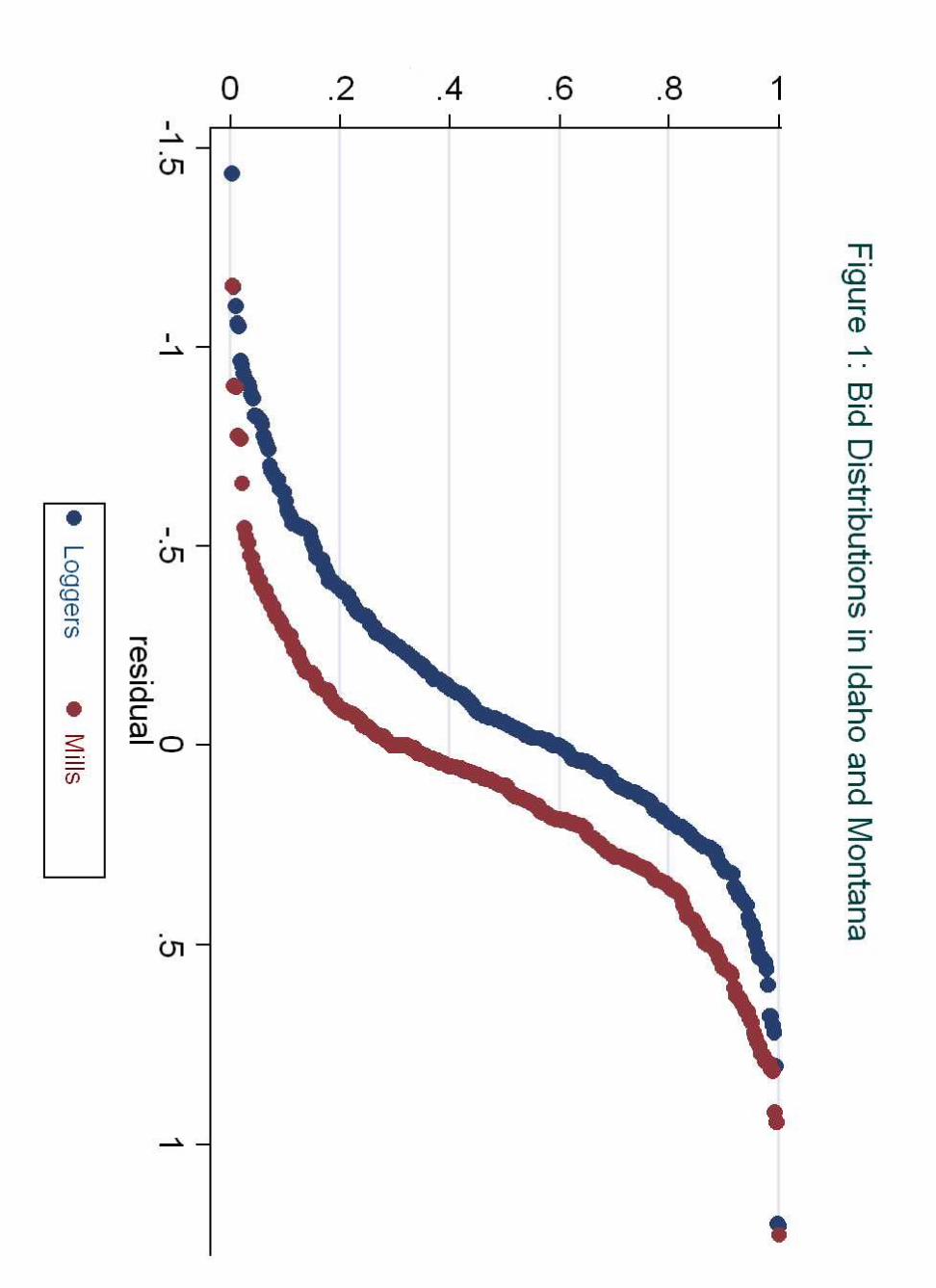
A second test is to compare the bids of mills and loggers. To do this, we focus on
(non-set aside) sealed auctions. We regress the per-unit bids of individual bidders (in
logs) on sale characteristics and consider the residuals from this regression. Figure 2
plots a smoothed cumulative distribution of the residuals for mills and loggers. The
cumulative distribution for mills lies to the right of that for loggers, indicating that
the bids of mills first order stochastically dominate those of loggers. To get a sense of
the magnitude of the difference, if one regresses log bids on sale characteristics and
a dummy for whether the bidder is a mill, the coefficient of the mill dummy is 0.396,
meaning mill bids are almost 40% higher on average, with a t-statistic above 10. Note
19

that Figure 2 plots the bid distributions conditional on entry. Because mills are also
more likely to enter, they also have higher unconditional bid distributions, which is
what is predicted by the model.
4. Comparing Auctions: Evidence
In this section, we investigate the consequences of auction choice for bidder par-
ticipation, revenue and allocation. We focus first on regular sales, then consider small
business sales. Our empirical approach is fairly straightforward; we describe it now
before turning to the specific questions.
A. Empirical Approach
Estimating the effect of auction method on different outcome variables is analogous
to estimating a policy “treatment effect.” An obvious strategy is to regress the relevant
outcome variable (e.g the number of entering mills or loggers, or the auction price
per unit) on a dummy variable indicating the auction method using a set of sale
characteristics as controls. To follow this approach, one estimates:
Y = α · SEALED + f(X) + ε,
where Y is the relevant outcome variable, SEALED a dummy equal to one if the
auction is sealed and zero if the auction is open, and X a vector of sale characteristics.
In our regressions, we include all of the sale characteristics used above to estimate
the choice of sale method.
This approach is easily interpretable, but there are caveats. The regression ap-
proach “partials out” the effect of sale characteristics on both the choice of auction
method and the auction outcome. If the functional form is mis-specified, the sealed
bid dummy may pick up residual correlation that we could mistake for a causal effect.
While our results do not seem very sensitive to the alternative control specifications
we have tried, this remains a potential concern.
For this reason, we also report a second set of estimates using a matching estima-
tor. This estimator matches every sealed auction with theM “closest” open auctions
20
and vice versa. The metric for matching is the weighted distance between sale char-
acteristics, where in addition to our standard set of characteristics, we include the
estimated propensity score for each auction. The estimated effect on outcome Y of
running a sealed bid rather than on open auction is:
∆Y =1
Ns
Xi,sealed
(Yi − Y oi ) +
1
No
Xi,open
(Y si − Yi),
where N τ is the number of sales of type τ ∈ {s, o} and Yi is the average outcome
of the M auctions of opposite format that are most similar to auction i in terms of
characteristics. We implement this estimator and compute standard errors following
Abadie and Imbens (2004), including using the regression method they suggest to
smooth imperfect matches.11
B. Bidder Participation
We start by looking at how auction choice affects the entry patterns of mills and
loggers. The competitive model suggests that controlling for sale characteristics, there
should be more entry by loggers and less entry by mills in sealed bid auctions. Table
3 reports our estimates of the effect of auction choice on bidder entry. Table 4 reports
more detailed results from the regression estimates.
The regression and matching estimates yield similar conclusions. Conditional on
other sale characteristics, the poisson regression estimate is that sealed bid auctions
attract roughly 38% more logger entrants than open auctions. Given a base level of
1.93 loggers in the open auctions, this translates into around 7-8 additional loggers
for every 10 sales, which is the same number we obtain with the matching estimator.
Sale format appears to have little effect on entry by mills once sale characteristics are
accounted for. The effect of auction format on mill entry is small and statistically
insignificant in both specifications.
The third column of Table 3 reports estimates of the effect of auction format
on the fraction of entrants who are loggers. Consistent with the entry results, the
composition of bidders at sealed bid auctions is shifted toward loggers. On average
11Our estimates appear to be somewhat sensitive to the choice of controls used in the bias-correction, but we have not had time to explore this in detail.
21

the fraction of participants who are loggers is 6-8% higher in sealed bid auctions than
in open auctions.
C. Auction Revenue
Our next step is to look at the effect of auction method on sale revenue, the issue
that has attracted the most attention among economists. The fourth column of Table
3 reports our estimate from regressing the log of the sale price per unit volume on sale
format and other sale characteristics, as well as the corresponding matching estimate.
The full regression specification is reported in Table 5.
We find that after conditioning on sale characteristics, sealed bid auctions raise
10-20% more revenue than open auctions for the average sale (10% is the matching
estimate; 20% is the regression estimate). To get a sense of the magnitude in dollar
terms, note that the average winning bid (in 1983 dollars rather than 1983 dollars
per unit volume) is around $320, 000. So a 10% difference in the winning bid price
translates into a $32, 000 difference in Forest Service revenue per sale, or about $15
million for the whole sample.
A natural question is whether the revenue difference is due to the fact that sealed
bid auctions attract more bidders. The second column of Table 5 reports estimates
of the winning bid where we include the number of entering loggers and mills as
covariates. The estimates suggest that an additional mill is associated with about a
15% increase in the winning bid, while and additional logger is associated with about
a 8% increase in the winning bid. Even controlling for the number of entrants, sale
method appears to matter; sealed bid auctions generate almost 14% more revenue.
The matching estimator suggests a smaller total revenue effect, but the decomposition
is similar.
We interpret this revenue decomposition with some caution because an obvious
concern is that there are sale characteristics that are observed by the bidders but
not accounted for in our data. In this case, the number of entrants is endogenous
in this regression. An approach followed in the auction literature is to instrument
for the number of entering bidders using measures of potential competition. We
have experimented with this, but are skeptical of the results for two reasons. First,
our estimated coefficients were highly sensitive to the particular choice of potential
competition measures. Second, potential competition measures are a valid instrument
22

only if entrants to a sealed auction perfectly observe the other entering bidders; if they
do not (as in our model) potential competition will have a direct effect on submitted
bids.
D. Allocation
A final prediction coming from the theoretical model is that sealed bid auctions
should be more likely to be won by loggers. As noted above, this comes across to
some extent in the raw data, and the patterns of entry documented above suggest it
is likely to be the case even after controlling for sale characteristics as the proportion
of entering bidders who are loggers is significantly greater in the sealed auctions.
Interestingly, however, we do not see a statistically significant difference in tract
allocation once we account for characteristics. Our estimates are reported in the final
column of Table 3. Using both a linear probability specification and the matching
estimator, we find the effect of auction format on allocation is fairly small and not
statistically distinguishable from zero. We will return to this finding below when we
try to piece together the evidence.
E. Small Business Sales
A substantial fraction of sales in the Idaho and Montana forests are small business
set-aside (SBA) sales. As noted above, this means that participation is restricted to
smaller firms. Table 1 contains summary statistics for these sales; there are 583 in
our sample. Though these sales attract on average a similar number of bidders as
the regular sales – between four and five – the set of participants is quite different.
There are very few mills participating. Nearly three quarter of the sales do not attract
any mill entrants (at least one mill enters in just 158 out of 583 sales). Moreover,
loggers win virtually all of the SBA sales. There are also substantial differences
between the tracts sold in regular and SBA sales. Notably, the SBA sales are generally
smaller and often do not involve road construction.
In terms of comparing auction methods, the small business sales are interesting
because the set of bidders is arguably far more homogenous than in the sales that
are open to all firms. The theory suggests that auction format should play a less
important role when bidders are homogenous.
23

According to Table 1, revenue, entry and allocation are in fact quite similar across
the two auction formats. However, the sets of tracts being compared are not iden-
tical; as with regular sales, the sealed bid sales are smaller on average. So a careful
comparison requires us to control for tract characteristics. Following the approach
above, we first estimate a logit regression to predict sale method. The estimates are
reported in Table 2; a smoothed histogram of the propensity scores appears in Figure
3. As above, we drop sales with propensity scores below 0.025 or above 0.975, leaving
us with 355 open and 192 sealed auctions, before estimating the effect of sale method
on outcome.
Table 6 presents our estimates of the effect of auction method on the various
outcome variables. The full results from the regression estimates are in Tables 7
and 8. Strikingly, we find no significant effects of auction method on either entry or
revenue. The average winning bids in sealed bid and open auctions, conditional on
sale characteristics, are within a quarter of a percentage point. Total entry is also very
similar. One estimate worth mentioning is that sealed bid auctions seem to attract
more mill entrants than open auctions (roughly 15% according to both estimates).
There is little mill entry in general, however, so this amounts to only one additional
mill every 13 sales. Moreover, this number is not estimated very precisely, so it is far
from being statistically significant.
F. Evidence from California Sales
All of the evidence we have discussed so far comes from two large forests in Idaho
and Montana. While these forests seem particularly well-suited to making a statistical
comparison between auction methods, we would like to have additional evidence to
draw on. To this end, we also examined sales from California forests in the Forest
Service’s Pacific Southwest Region. We consider sales that took place between 1982
and 1989. We have data on 1349 open auctions and 985 sealed bid auctions.
While the Forest Service sale process is similar in California and the set of potential
bidders includes both firms with manufacturing capability and logging companies,
this sample is somewhat less ideal. The reason, which can be seen in the summary
statistics in Table 9, is that the tracts sold by sealed bid auction tend to be quite
different from those sold by open auction. The principal difference is in the size of
sales. The average sale volume for the open auctions is nearly 6100 mbf, while it is
24

closer to 600 mbf for the sealed bid auctions. The sealed bid auctions are also much
more likely to be salvage sales. The per unit reserve prices are similar across sale
formats.
The final column of Table 2 reports a logit estimate of the choice of sale method,
using our standard controls. As is apparent in the summary numbers, volume is a
highly important correlate of sale method. Though our estimates do not appear in
the table, sale method also appears to vary significantly across the twelve forests in
the region. The extent to which sale method correlates with sale characteristics can
also be seen in Figure 4, where we plot the density of the propensity score for the
open and sealed bid auctions. Our logit regression predicts the sale method of many
of the open auctions with near-perfect precision; this is mainly a function of the fact
that very large sales are almost certain not to be sealed bid.
As with the Idaho and Montana data, we again drop sales that have an estimated
propensity score below 0.025 and above 0.975. This leaves us with 491 open auctions
and 603 sealed bid auctions. As can be seen in Table 9, the selected sample has some-
what smaller differences across sale format, but the open auctions are still notably
larger on average. This leads to two concerns about estimating the effect of auction
method on outcome. First, the relative paucity of large sealed sales and small open
sales will translate into less precise estimates. Second, if sale volume is independently
correlated with, for instance, revenue, a failure to flexibly control for sale volume
might lead us to falsely impute a revenue effect of auction method.
With these caveats in mind, we turn to Table 10, where we report our estimates
of the effect of auction method on entry, revenue and allocation outcomes. Details of
the regression estimates can be found in Tables 11 and 12. Though the magnitude of
the effects differ, the qualitative results are fairly similar to the Idaho and Montana
sales. Sealed bid auctions attract more loggers. The Poisson model gives an estimate
of 12% more loggers at sealed sales, which, given a base level of around 2 loggers per
sale, translates into an additional 2-3 loggers participating for every 10 sales. The
matching estimate is 4 additional loggers for every 10 sales. As is the case in Idaho
and Montana, we do not find much effect of sale method on mill participation. The
Poisson model predicts slightly fewer mills at sealed sales; the matching model slightly
more. Either way, the total number of participants, conditional on sale characteristics,
appears higher in sealed bid sales with the composition of bidders shifted toward
25

logging companies.
Our revenue estimates are also qualitatively similar to Idaho and Montana. We
find that after controlling for sale characteristics, the winning bid in sealed bid auc-
tions is around 8-9% higher than in open auctions. The average sale price for the
California sales is about $190,000 for our selected sample ($398,000 for the full sample,
reflecting the fact that we eliminated many of the largest sales), so an 8-9% revenue
difference across sale formats translates to about $16,000 per sale for the selected
sample. When we attempt to decompose this effect by controlling for the number of
entering bidders, our regression estimate is that about half of the difference in winning
bids is due to the increase in the number of participating bidders, while the difference
in winning bids across format after controlling for participating bidders is just over
4%. For the latter number, we get a more puzzling point estimate of 10% from the
matching estimator, which would suggest that additional entry reduces revenue.
One difference between the California results and those for Idaho and Montana
is the effect of sale method on the allocation. In the California sample, we find that
after controlling for sale characteristics, loggers are somewhat more likely to win with
a sealed format. The effect is not terribly large – it is 3% more likely a logger will
win with a sealed format according to our matching estimate, 6% according to the
linear probability model – with moderate statistical significance under the linear
model.
5. Assessing the Evidence
In this section, we assess the extent to which our empirical findings square with
the competitive bidding model developed earlier in the paper. We argue that the
competitive model can explain a number of the findings, but does not provide a
perfect fit with the data. We then discuss alternative explanations for our findings,
and some caveats and limitations to our results.
A. How Does the Competitive Model Fare?
Our empirical evidence suggests that in both the two large Idaho and Montana
forests, and in the California forests, there are significant differences between the
outcomes of sealed bid and open auctions. The two most notable differences concern
26
participation and revenue. Conditional on sale characteristics, sealed bid auctions
attract more entry by logging companies, with negligible changes in the entry of mills,
who appear to be substantially stronger bidders. The winning bids in the sealed bid
sales we observe are also appreciably higher: 10-20% higher in Idaho and Montana
after controlling for sale characteristics, and 8-9% higher in California. Sale method
does not appear to significantly influence the probability that a logging company
will win the sale in Idaho and Montana, though it may increase it somewhat in
the California data. When we consider small business set-aside sales, all of these
differences disappear and sealed bid and open auctions appear extremely similar in
terms of participation and revenue.
The competitive bidding model we developed earlier in the paper is consistent
with many, but not all, of these findings. For the regular sales, the bidding model
predicts that sealed bid sales will result in more entry by loggers, and higher winning
bids, as well as a increase in the probability that a logger will win the auction. For the
small business sales, one interpretation of the results is that the bidders in these sales
– nearly all loggers – are relatively homogenous. In this case the model accurately
predicts no differences in the outcomes of open and sealed bid auctions.
There are several points, however, where the model does not immediately fit the
data. For instance, the model predicts less participation by mills in sealed bid sales,
while we see no effect. This is not terribly hard to reconcile with the theory. If there
are relatively few mills and their participation is driven primarily by large shifts
that are independent of the auction format — such as inventory levels or available
manpower, it may well be the case that for any given sale, some mills are simply
uninterested, while others want to enter regardless of sale format. So a change in
sale format simply has no effect on observed mill participation. In contrast, there
are more logging companies, so if participation is a more marginal decision, we would
expect more logger entry in sealed bid auctions and consequently higher prices.
A discrepancy that is more troubling for the theory is that in Idaho and Montana,
it is no more likely that a sealed sale will be won by a logging company than an open
auction sale. This is an important prediction of the model that is not borne out in
the data. Finally, and we will return to this point in a more substantive way, the
revenue differences in Idaho and Montana strike us as perhaps larger than one might
expect from an asymmetric private values bidding model. This suggests that we need
27
to consider alternative explanations for our findings, both as a check on our positive
findings and as a way to resolve discrepancies.
B. Alternative Explanations
A simple alternative explanation for why we see more logger participation in sealed
bid auctions, but not notably less mill participation is that the costs of entering a
sealed bid auction are lower than the costs of entering an open auction. This would
also help to explain the revenue differences, although as we saw above participation
appears to account for only about half of these. However, while it seems plausible in
some contexts that sealed bidding would lower participation costs, the cost difference
here seems limited to a day spent traveling to the auction, which is probably small
given that winning bids are in the hundreds of thousands of dollars for an average sale.
Moreover, a large difference in transaction costs across formats would presumably lead
to differences at small business sales as well.
Another explanation for our findings is that our estimates do not reflect systematic
behavioral difference across the two formats, or that the true behavioral differences
are masked by endogeneity problems. Instead, our estimates reflect the fact that
we have not adequately controlled for auction characteristics that influence both the
choice of sale method and auction outcomes. This is certainly a concern. Even in
Idaho and Montana, where we know that many sale assignments were random, there
are observable differences across the set of open and sealed bid sales. And as we have
noted the differences are much greater in California. We have attempted to mitigate
this by making use of the very rich data on sale characteristics in the Forest Service
sale reports, augmented by further data on market conditions.
Is there a plausible omitted variable story that might generate our findings? Sev-
eral of the most obvious stories have problems themselves. For instance, one possibil-
ity is that forest managers like to sell more valuable tracts by sealed bid, a bias that
would help to explain the entry and revenue differences we find. This story is hard to
square, however, with both the SBA data and with the fact that larger sales, which
are by definition more valuable on a total value basis, are more often sold by open
auction. A second possibility is that forest managers use sealed bid sales when they
expect there to be more bidder interest, especially on the part of logging companies.
This would certainly help to explain the entry results, though it is not clear to us
28

why forest managers would systematically behave in this way (unless, for instance,
loggers had a preference for sealed bidding as in the model).
A final possibility given our findings is that competition in the industry is not
perfectly competitive, but rather there is some degree of tacit cooperation, particu-
larly among the mills and at the oral auctions. The possibility of tacit cooperation at
Forest Service timber auctions has been noted by Mead (1967) and Baldwin, Marshall
and Richard (1997) and it is a widely-held view that collusion is easier to sustain at
oral auctions, where the bidders are face to face and can respond to each other’s ac-
tions. It is not entirely clear why tacit cooperation would generate the entry patterns
we observe, or why there would be no revenue differences for the SBA sales. One
possibility is that tacit cooperation occurs mainly between the mills and at the larger
sales (which are more likely to be open auctions). This could potentially account for
the large revenue differences across format.
6. Structural Tests of the Competitive Model
[To be written...]
7. Conclusion
This paper has examined the relative performance of open and sealed bid auctions,
using U.S. Forest Service timber sales as a test case in auction design. We find
that when bidders are relatively homogenous, there is little difference between the
outcomes of open and sealed bid auctions. When bidders are heterogenous, however,
sealed bid auctions encourage the entry of weaker bidders and result in higher revenue.
The former finding is consistent with the revenue equivalence theorem, while the
latter fits reasonably well with our extension of the standard private value model of
competitive bidding.
Appendix: Proofs of the Results
29

We provide detailed proofs of our theoretical results. Our basic proof techniqueis to consider the bidding equilibrium in a game where entry thresholds are exoge-nously fixed and bids are the only strategic choice and then from there characterizeequilibrium of the complete entry and bidding game.
A. Existence of Monotone Entry Equilibrium
To begin, we establish existence of a monotone entry equilibrium.
Proposition 7 For both auction rules, a monotone entry equilibrium exists.
Proof. For the sealed bid auction, the results of Li and Riley (1999) can be adapted toshow that for any fixed set of entry thresholds,K1, ...,Kn, there is a unique equilibriumin the game where player select only bidding strategies. The same is true for the openauction if we restrict attention to undominated strategies because bidding one’s truevalue is a dominant strategy. We use these facts to establish an entry equilibrium.The proof is the same for both auction formats. Given a set of entry thresholds
K = (K1, ...,Kn), and the induced equilibrium bidding strategies, let Πi(K) denote ı’sprofits from participating in the auction. An entry equilibrium is a vector K, coupledwith the induced equilibrium bidding strategies, such that for all i:
πi(K) := min{Πi(K), k} = Ki.
Establishing a (monotone) entry equilibrium amounts to finding a (monotone) fixedpoint of π = (π1, ..., πn). We will use Kakutani’s fixed point theorem to do this.Consider the space of monotone thresholds:
K = {(K ∈ [0, k]n : K1 ≥ ... ≥ Kn}.
This space is a compact convex subset of Rn. Because a bidding equilibrium existsand is unique for all K, π(·) is non-empty and single-valued. Moreover, because Π(·)is a vector of Nash equilibrium payoffs, it is upper semi-continuous in K, and hencecontinuous because it is a function. Therefore π(·) is continuous in K. Finally, weprove below (Claim 3 in the two following sections) that if K1 ≥ ... ≥ Kn, thenΠ1(K) ≥ ... ≥ Πn(K). So π : K → K, and by Kakutani’s theorem has a fixed pointin K.12 Q.E.D.
B. Characterization of Sealed Bid Equilibrium.
12Note that our proof does not establish the existence of a symmetric equilibrium if bidders haveidentical value distributions, or of a type-symmetric equilibrium if there are only two types of bidders,but it is easy to do so with minor changes to the argument.
30

For anyK1 ≥ ... ≥ Kn, we consider the induced bidding equilibrium b1(·), ..., bn(·).We establish a set of results about these bid strategies and the corresponding biddistributions G1, ..., Gn. These results hold for the bidding equilibrium induced byany set of monotone entry thresholds K1, ..., Kn, so they also hold at any monotoneentry equilibrium.
1. (Equilibrium) For every bidder i, value vi ≥ r and equilibrium bid b = bi(vi):
1
vi − b=Xj 6=i
gj(b)
Gj(b). (8)
Moreover, bi(·) is continuous and strictly increasing for vi ≥ r and Gi is contin-uous and strictly increasing on the interval [r, bi], where bi = bi(vi).
Proof. First, note that i can’t bid an atom at some b because then no other bidderwould bid just below b, meaning i couldn’t optimally bid b. So Gi is continuous forall i above the reserve price. Conditional on entry, bidder i solves:
maxb(vi − b)
Yj 6=i
Gj(b),
so (8) is the first order condition. The optimizer bi(·) is nondecreasing by Topkis’Theorem and must be strictly increasing because Gi is continuous. Finally, each bi(·)is continuous from the first order condition, so Gi must be strictly increasing on [r, bi].Q.E.D.
2. (Monotonicity) For all i and b ≥ r, Gi(b) ≤ Gi+1(b) (with strict inequality ifFi < Fi+1 at the relevant v or if Ki > Ki+1).
Proof. We first show that bi ≥ bi+1. Suppose not so that bi < bi+1. Then ifb = bi+1(vi+1) is just above bi,
1
vi − b>Xj 6=i
gj(b)
Gj(b)>Xj 6=i+1
gj(b)
Gj(b)=
1
vi+1 − b.
But this implies that vi+1 > vi, a contradiction. So bi is nonincreasing in i andGi(b) ≤ Gi+1(b) for all b ≥ bi+1.Now, suppose for some b, Gi(b) ≥ Gi+1(b) > 0. Define vi and vi+1 so that
bi(vi) = bi+1(vi+1) = b. Observe that:
Gi(b) := 1−Hi +HiFi(b−1i (b)), (9)
31

where b−1i (0) := bi, and Hi := H(Ki). Because Hi ≥ Hi+1 , it follows from (9) thatFi(vi) ≥ Fi+1(vi+1). By Assumption (ii), this means that vi ≥ vi+1. Consequentlyfrom (8), (g/G)i(b) ≥ (g/G)i+1(b) and hence gi(b) ≥ gi+1(b).Therefore, because Gi(bi+1) ≤ Gi+1(bi+1) = 1, we have Gi(b) ≤ Gi+1(b) for all
b ∈ [r, b]. The inequality is strict if Fi < Fi+1 at the relevant v or if Hi > Hi+1.Q.E.D.
3. (Profits) Conditional and unconditional bidder profits Πsi (v;K) and Πs
i (K) arenonincreasing in i.
Proof. Bidder i’s profits, conditional on entry and having a value v ≥ r, are:
Πsi (v;K) := max
b≥r(v − b)
Yj 6=i
Gj(b).
By the envelope theorem, profits are increasing in v. Moreover, for all b,Q
j 6=iGj(b)
is nonincreasing in i, so Πi(v) is nonincreasing in i. Finally, because Fi(·) ≤ Fi+1(·),bidder i + 1 will have higher profits than i in expectation conditional on entry andhence unconditionally. Q.E.D.
4. (Bid Shading) For all i and v, bi(v) ≤ bi+1(v).
Proof. First note if bi(v) > bi+1(v) for some v, then equivalently there is some b forwhich vi = b−1i (b) < b−1i+1(b) = vi+1. Suppose this is the case for some b. From thefirst order conditions:
gi(b)
Gi(b)<
gi+1(b)
Gi+1(b).
Note that this b cannot be in the neighborhood of b. Because Gi(b) = Gi+1(b) = 1,this would imply that Gi > Gi+1 near b, a contradiction. So for values of v near v,bi(v) ≤ bi+1(v).Now, suppose there is some b such that v = b−1i (b) = b−1i+1(b). For this b,
(g/G)i(b) = (g/G)i+1(b). From (2), this means that:
Hifi(v)
1−Hi +HiFi(v)(b−1i )
0(b) =Hi+1fi+1(v)
1−Hi+1 +Hi+1Fi+1(v)(b−1i+1)
0(b).
Using the maintained hypothesis that Hi ≥ Hi+1, and noting that Hi = H(Ki) ≥H(0) = ϕ for all i, we can re-arrange assumption (iii) to show that:
Hifi(v)
1−Hi −HiFi(v)≥ Hi+1fi+1(v)
1−Hi+1 +Hi+1Fi+1(v).
32

Therefore (b−1i )0(b) ≤ (b−1i+1)0(b). It follows that just below b, b−1i (b) ≥ b−1i+1(b). Or in
other words, just below v, bi(v) ≤ bi+1(v). Q.E.D.
Characterization of Open Auction Equilibrium
Next we look at open auction equilibria. Again we fix a set of monotone entrythresholds K1 ≥ ... ≥ Kn and consider the induced equilibrium bidding strategiesb1(·), ..., bn(·). Note that as the results hold for any monotone K, they hold at anymonotone entry equilibrium.
1. (Equilibrium) Every bidder i has a (weakly) dominant bidding strategy bi(v) = v.
2. (Monotonicity) For all i and b, Gi(b) ≤ Gi+1(b) (with strict inequality if Fi < Fi+1
at the relevant v or if Ki > Ki+1).
Proof. Given that: Gi(b) := 1−Hi+HiFi(b), this follows immediately from the factthat H1 ≥ ... ≥ Hn and Fi(b) ≤ ... ≤ Fn(b) for all b. Q.E.D.
3. (Profits) Bidder profits, Πoi (K) are nonincreasing in i. Moreover, Π
oi (K) is constant
in Ki and decreasing in Kj for all j 6= i.
Proof. The first statement follows from the fact that i faces weaker competition thani + 1 because Gi(·) ≤ Gi+1(·). For the second part, observe that an increase in Ki
will not affect Gj for any j 6= i so it won’t affect Πi, while an increase in Kj will shiftGj up in the sense of first order stochastic dominance, so it will decrease Πi. Q.E.D.
D. Comparing Auctions
We now provide proofs of our results comparing the two auction formats. Asnoted earlier, the key is to use the envelope theorem representation of bidder profits.For auction type τ ∈ {s, o}, given monotone entry cost thresholds K1 ≥ ... ≥ Kn andthe induced equilibrium bidding strategies, we have:
Πτi (vi;K) =
Z v
v
Pr[i wins | vi = x;K]dx.
The probability that i wins given a value v is:
Pr[i wins|v;K] :=Yj 6=i
Gj(bi(v)) =Yj 6=i
©1−Hj +HjFj(b
−1j (bi(v))
ª,
where Hj := H(Kj), and bj is the appropriate induced equilibrium bid strategy.
33

Proof of Proposition 3. (Revenue Equivalence). Suppose bidders have identicalvalue distributions and use identical entry strategies Ki = K for all i. For the sealedbid auction, there is a unique symmetric equilibrium in the induced bidding game.In equilibrium, bidder i wins if and only if he has the highest value of the entrants.The same is true in the open auction. Therefore for and K = (K, ...,K) and acorresponding symmetric equilibrium in bid strategies, we have Πs
i (K) = Πoi (K).
Moreover, Πoi is constant inKi and decreasing inKj, so it is decreasing inK whenK =
(K, ...,K). It follows immediately that there is a unique symmetric entry equilibriumfor both the open and sealed auction, where the symmetric entry threshold solvesΠτi (K, ...,K) = min{k,K}. It follows immediately that expected entry is the samein the open and sealed bid auctions. Moreover, as the highest valued entrant wins,social surplus is the same across auctions as are bidder profits. The expected revenueis just the difference between expected social surplus and expected bidder profits, soit too must be the same across auction formats.
For the remaining results, the following Lemma is useful.
Lemma 1 For any set of entry cost thresholds K1 ≥ ... ≥ Kn, if we compare theinduced equilibrium in bid strategies in the open and sealed bid auction, the strongestbidder 1 makes higher profits in the open auction while the converse is true for theweakest bidder n.
Proof of Lemma 1. From above, we know that in the sealed bid equilibriumb1(v) ≤ ... ≤ bn(v) for all v ≥ r. Therefore for any v ≥ r
Pr[1 wins | v1, K, Open] ≥ Pr[1 wins | v1, K, Sealed],
while the converse holds for bidder n. Therefore Πo1(v1;K) ≥ Πs
1(v1;K) and conse-quently Πo
1(K) ≥ Πs1(K), while the converse holds for bidder n. Q.E.D.
The remaining Propositions all apply to the specialized case of two types of biddersand type-symmetric equilibria.
Proof of Proposition 4. (Entry) Consider a sealed bid entry equilibrium withK1 ≥ ... ≥ Kn. We show there must be an entry equilibrium of the open auctionwhere strong bidders are more likely to enter (K1 increases) and weak bidders are lesslikely to enter (Kn decreases).We start with a graphical depiction of entry equilibrium for the open auction.
Define:πi(K) := min{Πo
i (K), k}−Ki.
34

Consider the space {(K1,Kn) : Ki ∈ [0, k]}. As we are interested in type-symmetricequilibria, a pair (K1,Kn) fully describes a vector of entry thresholds for all thebidders. Now, consider the locus of points (K1,Kn) for which πi(K) − Ki = 0.Denote this locus as Li. These curves L1,L2 are depicted in Figure 1.
00
k
k
K1
Kn
K1=Kn
π1(K)–K1=0
Ko
Ks
πn(K)–Kn=0
Entry Equilibrium in Open Auction
Several points are important. First, both curves are continuous. Second, bothcurves are downward sloping because Πo
i (·) and hence πi(·) is decreasing inK. There-fore, above Li, πi(K)−Ki < 0 while below Li, πi(K)−Ki > 0. Third, if K1 = Kn,then Πo
1(K) > Πon(K). Therefore L1 intersects the 45 degree line above Ln. Fourth, if
Ki = 0, then because Π0i ≥ 0, πi(K)−Ki ≥ 0, while if Ki = k, then πi(K)−Ki ≤ 0
by definition. Therefore, L1 lies above Ln at K1 = 0 and below it at K1 = k.Any intersection of the curves L1 and Ln is an entry equilibrium of the oral auction.
In the game depicted in the figure, there is a unique equilibrium, but in general theremay be several. We know from the proposition above, and also from the points inthe previous paragraph than at least one equilibrium lies below the 45 degree lineand is monotone. Moreover, it is easy to see that given any point K = (K1,Kn)that lies above L1 and below Ln, there must be an oral auction equilibrium Ko withKo1 ≥ K1 and Ko
n ≤ Kn.With these preliminaries, we are ready to prove the result. From Lemma 1, we
know that for any monotone K:
Πo1(K) ≥ Πs
1(K)
Πon(K) ≤ Πs
n(K).
35

Let Ks denote the sealed monotone entry equilibrium. Suppose that Ks is interior(the proof is essentially the same if Ks is on the boundary of K). Then
π1(Ks)−Ks
1 ≥ 0
πn(Ks)−Ks
n ≤ 0.
Therefore Ks lies above L1, below Ln, and to the right of the 45 degree line (asillustrated in Figure 1). Therefore there must be some open auction equilibrium Ko
with Ko1 ≥ Ks
1 and Kon ≤ Ks
n.Note that weak bidders are more likely to win in the sealed bid equilibrium.
By the bid shading result above, weak bidders would be more likely to win in asealed bid auction with entry exogenously given by Ko than in the open auction withequilibrium entry. Therefore they are even more likely to win in the sealed bid auctionwith equilibrium entry Ks. Q.E.D.
Proof of Proposition 5. (Efficiency) For an exogenous set of entry thresholds,the open auction will allocate the item efficiently; the sealed auction will not (atleast in expectation). Moreover, in an oral auction each bidder obtains his marginalcontribution to social surplus (or his Vickrey profit). So the equilibrium entry thresh-olds are (locally) efficient in the sense that a social planner could not increase socialsurplus by changing Ki while holding K−i fixed. Indeed every local optimum of theplanner’s entry choice problem is an equilibrium of the oral auction entry game, sothe global optimum is an equilibrium. As this equilibrium maximizes social surplus, itmust generate strictly more surplus than any equilibrium of the sealed auction game,provided that there is at least some asymmetry between the two types of bidders.Q.E.D.
Proof of Proposition 6. (Competition) Consider some bidder i. The uncon-ditional probability that i will bid at least b is 1 − Gi(b). Conditional on entry,the probability is 1 − Fi(b
−1i (b)) ≥ 1 − Gi(b) with strict inequality provided that
H(Ki) < 1. Therefore the additional entry of any bidder raises expected revenue.Q.E.D.
References
Abadie, A. and G. Imbens, “Large Sample Properties of Matching Estimatorsfor Average Treatment Effects,” UC Berkeley Working Paper, 2004.
Athey, S. and J. Levin, “Information and Competition in U.S. Forest ServiceTimber Auctions,” Journal of Political Economy, April 2001, 109(2), pp. 375—417.
36

Baldwin, L., R. Marshall, and J.-F. Richard., “Bidder Collusion at U.S. ForestService Timber Auctions,” Journal of Political Economy, August 1997, 105(4),pp. 657—699.
Bulow, J. and P. Klemperer, “Prices and the Winner’s Curse,” Rand Journal ofEconomics, Spring 2002, 33(1), pp. 1—21.
Guerre, E., I. Perrigne and Q. Vuong, “Optimal Nonparametric Estimation ofFirst Price Auctions,” Econometrica, May 2000, 68(3), pp. 525—574.
Haile, P., “Auctions with Resale Markets: An Application to U.S. Forest ServiceTimber Sales,” American Economic Review, June 2001, 92(3), pp. 399—427.
Haile, P., H. Hong and M. Shum, “Nonparametric Tests for Common Valuesin First-Price Sealed Bid Auctions,” Yale University Working Paper, 2003.
Hansen, R., “Sealed-Bid Versus Open Auctions: The Evidence,” Economic Inquiry,January 1986, 24(1), pp. 125—142.
Johnson, R., “Oral Auctions versus Sealed Bids: An Empirical Investigation,”Natural Resources Journal, April 1979, 19(2), pp. 315—335.
Kagel, J., “Auctions: A Survey of Experimental Research,” in The Handbook ofExperimental Economics, edited by J. Kagel and A. Roth, Princeton UniversityPress, 1995.
Li, H. and J. Riley, “Auction Choice,” UCLA Working Paper, 1999.
Lucking-Reilly, D., “Using Field Experiments to Test Equivalence Between Auc-tion Formats: Magic on the Internet,” American Economic Review, December1999, 89(5), pp. 1063-1080.
Maskin, E. and J. Riley, “Asymmetric Auctions,” Review of Economic Studies,July 2000, 67(3), pp. 413—438.
Mead, W., “Natural Resource Disposal — Oral Auction Versus Sealed Bids,” Nat-ural Resources Journal, April 1967, 7(2), pp. 194—224.
Milgrom, P., Putting Auction Theory to Work, Cambridge University Press, 2004.
Robinson, M., “Collusion and the Choice of Auction,” Bell Journal of Economics,Spring 1985, 16(1), pp. 141-145
37
Rosenbaum, P. and D. Rubin, “The Central Role of the Propensity Score inObservational Studies for Causal Effects,” Biometrika, 1983, 70, pp. 41—55.
Schuster, E. and M. Niccolucci, “Sealed-Bid Versus Oral-Auction Timber Of-ferings: Implications of Imperfect Data,” Canadian Journal of Forest Research,1994, 24, pp. 87—91.
Stone, J. and D. Rideout, “Does Sealed Bidding Promote Competition in theAuctioning of Public Timber?” Journal of Forest Economics, 1997, 3(2), pp.133—142.
Vickrey, W., “Counterspeculation, Auctions and Sealed Tenders,” Journal of Fi-nance, 1961, 16, pp. 8—37.
38

Open A
uctionsO
pen Auctions
Sealed Bid
Full Sample
SelectedFull
FullN
432345
389194
Mean
Std. Dev.
Mean
Std. Dev.
Mean
Std. Dev.
M
eanStd. D
ev.M
eanStd. D
ev.A
uction Outcom
esW
inning Bid ($/m
bf)79.80
56.7984.21
58.12103.63
68.8659.50
45.4964.43
36.91E
ntrants4.14
2.354.30
2.414.85
2.714.21
2.624.38
2.90 # Loggers E
ntering1.76
2.121.93
2.212.67
2.323.74
2.423.99
2.68 # M
ills Entering
2.381.64
2.371.70
2.181.95
0.470.88
0.390.82
Logger Wins A
uction0.18
0.390.20
0.400.25
0.440.98
0.120.98
0.14
Appraisal Variables
Volum
e of timber (hundred m
bf)43.77
45.6638.80
43.0625.84
35.7612.54
21.707.03
12.94R
eserve Price ($/m
bf)27.07
25.6028.57
26.5828.68
25.0925.22
27.5727.48
22.98R
oad Construction ($/m
bf)8.83
11.057.99
11.165.80
10.273.78
8.131.07
4.14N
o Road C
onstruction0.43
0.500.48
0.500.61
0.490.75
0.430.90
0.30
Sale Characteristics
Contract Length (m
onths)32.12
18.8530.33
19.1324.34
18.0816.77
11.3813.42
9.31S
pecies Herfindal
0.530.25
0.510.24
0.500.22
0.660.28
0.610.28
Density of Tim
ber (acres/hmbf)
28.8928.50
27.6226.83
34.6956.44
36.3681.76
36.2351.18
Salvage S
ale0.34
0.470.34
0.480.44
0.500.44
0.500.40
0.49
Potential Com
petitionLogging com
panies in county38.62
21.6536.77
21.7335.00
22.1547.75
20.2141.60
22.09S
awm
ills in County
8.094.74
8.005.08
7.114.48
9.204.19
7.674.40
Table 1: Summ
ary Statistics for Idaho/Montana (R
egion 1) Sales
Sealed Bid
Full/Selected130
Small B
usiness (SBA
) SalesR
egular Sales

Table 2: Choice of Sale MethodDependent Variable: Dummy if auction is sealed bid (Logit regression)
(1) (2) (3) Region 1: Non-SBA Region 1: SBA Region 5: Non-SBA
coefficient s.e. coefficient s.e. coefficient s.e.
Appraisal ControlsLn(Reserve Price) -0.278 (0.198) -0.088 (0.175) 0.266 (0.170)Ln(Selling Value) 0.060 (0.103) -0.119 (0.086) -1.849 (0.756)*Ln(Logging Costs) 1.865 (0.971) -0.185 (0.627) -0.636 (0.567)Ln(Manufacturing Costs) 0.641 (1.334) 1.027 (0.948) 0.158 (0.253)Ln(Road Costs) 0.173 (0.273) -0.570 (0.463) -0.097 (0.215)No Road Construct. (Dummy) 0.360 (0.741) -0.411 (1.134) 0.307 (0.552)
Volume Controls (Dummy Variables):Volume: 1.5-3 hundred mbf 2.037 (1.344) -0.484 (0.451) -0.200 (0.453)Volume: 3-5 0.975 (1.388) -0.571 (0.484) -0.977 (0.481)*Volume: 5-8 0.885 (1.361) -0.553 (0.536) -1.351 (0.501)**Volume: 8-12 0.069 (1.381) -1.068 (0.596) -2.166 (0.551)**Volume: 12-20 0.466 (1.393) -1.382 (0.663)* -2.654 (0.596)**Volume: 20-40 -0.469 (1.446) -2.325 (0.925)* -6.835 (0.721)**Volume: 40-65 -0.745 (1.496) -2.022 (1.185) -7.453 (0.778)**Volume: 65-90 -0.671 (1.581) -0.637 (1.491) -7.669 (0.811)**Volume: 90+ -1.384 (1.594) -2.891 (1.522) -8.945 (0.949)**
Potential Competitionln(Loggers in County) -0.666 (0.510) -0.112 (0.453) -0.492 (0.297)ln(Sawmills in County) 0.809 (0.487) -0.404 (0.542) 0.556 (0.298)ln(Lagged Mill Volume) -0.095 (0.073) -0.015 (0.062) 0.028 (0.046)ln(Lagged Logger Volume) 0.055 (0.107) -0.261 (0.096)** -0.032 (0.062)
Other Sale Characteristics Density of Timber (acres/hmbf) 0.005 (0.004) 0.000 (0.002) -0.000 (0.000)Species Herfindal -0.172 (0.863) 0.818 (0.783) -0.831 (0.513)Salvage Sale (Dummy) 0.428 (0.316) -0.003 (0.268) 0.329 (0.253)ln(Monthly US House Starts) -0.714 (1.734) -0.706 (1.517) -4.319 (1.283)**ln(Contract Length/volume) -0.457 (0.584) -0.279 (0.328) 0.387 (0.298)Constant -8.369 (14.071) 4.500 (11.665) 47.352 (10.094)**
Additional Controls: Year, Quarter, Species, District (Forest in California) dummies
N=562 N = 697 N=2334LR chi2 (68 129.51 LR chi2 (69 195.04 LR chi2 (69 2295.57Prob > chi2 0.000 Prob > chi2 0.000 Prob > chi2 0.000Pseudo-R2 0.221 Pseudo-R2 0.265 Pseudo-R2 0.7225

Dependent Variable:
Logger EntryM
ill EntryLoggers/Entrants
ln(Revenue)
ln(Revenue)*
Logger Wins
PoissonPoisson
Linear Reg.
Linear Reg.
Linear Reg.
Linear Reg.
Sealed B
id Dum
my
1.3821.035
0.0750.195
0.137-0.014
(0.112)***(0.081)
(0.027)***(0.053)***
(0.048)***(0.037)
See tables 4 and 5 for tull set of controls and coefficients. N
ote: Poisson coefficient is incidence rate.
Dependent Variable:
Logger EntryM
ill EntryLoggers/Entrants
ln(Revenue)
ln(Revenue)*
Logger Wins
Matching
Matching
Matching
Matching
Matching
Matching
Sealed B
id Dum
my
0.7750.066
0.0600.104
0.048-0.064
(0.250)***(0.060)
(0.032)*(0.058)*
(0 .061)(0.042)
Num
ber of matches = 4 using sam
e controls and estimated propensity score and A
badie-Imbens (2004) bias-correction.
*Note: specification includes num
ber of entering mills and loggers in addition to sale controls.
Table 3: Effect of Auction M
ethod on Sale Outcom
es (Idaho and Montana Sales)
Panel A: R
egression Estimates
Panel B: M
atching Estimates
(N=474 Sales)

Table 4: Entry in Idaho/Montana Sales (1) (2) (3) # Logger Entrants # Mill Entrants # Loggers/ # Entrants
Poisson Poisson Linear RegressionInc. Rate s.e. Inc. Rate s.e. coeff. s.e.
Sale MethodSealed Bid Auction 1.382 (0.112)** 1.035 (0.081) 0.075 (0.027)**
Appraisal Controls*Ln(Reserve Price) 0.790 (0.042)** 1.124 (0.064)* -0.086 (0.019)**Ln(Selling Value) 0.951 (0.027) 0.967 (0.028) -0.009 (0.009)Ln(Logging Costs) 0.242 (0.062)** 0.596 (0.186) -0.110 (0.091)Ln(Manufacturing Costs) 1.860 (0.603) 1.329 (0.560) 0.041 (0.114)Ln(Road Costs) 0.803 (0.076)* 0.960 (0.059) -0.024 (0.024)No Road Construct. (Dummy) 0.869 (0.209) 1.012 (0.172) -0.027 (0.065)
Volume Controls (Dummy Variables):Volume: 1.5-3 hundred mbf 2.342 (0.910)* 1.908 (1.463) -0.011 (0.119)Volume: 3-5 2.447 (0.944)* 4.039 (3.001) -0.194 (0.122)Volume: 5-8 1.845 (0.714) 5.468 (4.028)* -0.240 (0.120)*Volume: 8-12 2.010 (0.785) 6.648 (4.935)* -0.255 (0.124)*Volume: 12-20 1.807 (0.711) 11.104 (8.243)** -0.422 (0.125)**Volume: 20-40 1.071 (0.444) 13.055 (9.860)** -0.601 (0.132)**Volume: 40-65 0.952 (0.404) 14.273 (10.869)** -0.649 (0.136)**Volume: 65-90 0.523 (0.242) 16.358 (12.706)** -0.768 (0.144)**Volume: 90+ 0.534 (0.247) 21.025 (16.395)** -0.781 (0.146)**
Potential Competitionln(Loggers in County) 0.654 (0.090)** 1.085 (0.161) -0.104 (0.048)*ln(Sawmills in County) 1.467 (0.185)** 0.971 (0.124) 0.060 (0.044)ln(Lagged Mill Volume) 0.990 (0.020) 0.969 (0.019) 0.005 (0.007)ln(Lagged Logger Volume) 1.003 (0.030) 0.989 (0.028) 0.008 (0.010)
Other Sale CharacteristicsDensity of Timber (acres/hmbf) 0.999 (0.001) 0.999 (0.001) 0.000 (0.000)Species Herfindal 1.058 (0.261) 0.652 (0.151) 0.094 (0.079)Salvage Sale (Dummy) 1.251 (0.106)** 0.816 (0.075)* 0.128 (0.031)**ln(Monthly US House Starts) 2.250 (1.023) 1.612 (0.723) 0.032 (0.157)ln(Contract Length/volume) 1.055 (0.161) 1.455 (0.303) -0.067 (0.057)Constant 1.518 (1.245)
Additional Controls: Year, Quarter, Species, District dummies
N=475 N=475 N=475LR chi2 (68 604.86 LR chi2 (68 417.06 F(68, 475) 10.01Prob>chi2 0.000 Prob>chi2 0.000 Prob > F 0.000Pseudo-R2 0.292 Pseudo-R2 0.226 R-squared 0.627
* Note: All appraisal variables are per-unit volume, i.e. in $/mbf.
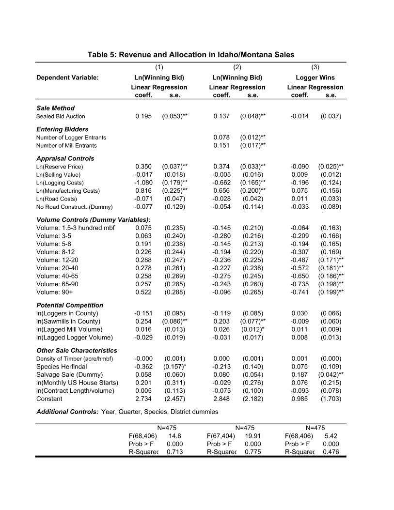
Table 5: Revenue and Allocation in Idaho/Montana Sales (1) (2) (3)Dependent Variable: Ln(Winning Bid) Ln(Winning Bid) Logger Wins
Linear Regression Linear Regression Linear Regressioncoeff. s.e. coeff. s.e. coeff. s.e.
Sale MethodSealed Bid Auction 0.195 (0.053)** 0.137 (0.048)** -0.014 (0.037)
Entering BiddersNumber of Logger Entrants 0.078 (0.012)**Number of Mill Entrants 0.151 (0.017)**
Appraisal ControlsLn(Reserve Price) 0.350 (0.037)** 0.374 (0.033)** -0.090 (0.025)**Ln(Selling Value) -0.017 (0.018) -0.005 (0.016) 0.009 (0.012)Ln(Logging Costs) -1.080 (0.179)** -0.662 (0.165)** -0.196 (0.124)Ln(Manufacturing Costs) 0.816 (0.225)** 0.656 (0.200)** 0.075 (0.156)Ln(Road Costs) -0.071 (0.047) -0.028 (0.042) 0.011 (0.033)No Road Construct. (Dummy) -0.077 (0.129) -0.054 (0.114) -0.033 (0.089)
Volume Controls (Dummy Variables):Volume: 1.5-3 hundred mbf 0.075 (0.235) -0.145 (0.210) -0.064 (0.163)Volume: 3-5 0.063 (0.240) -0.280 (0.216) -0.209 (0.166)Volume: 5-8 0.191 (0.238) -0.145 (0.213) -0.194 (0.165)Volume: 8-12 0.226 (0.244) -0.194 (0.220) -0.307 (0.169)Volume: 12-20 0.288 (0.247) -0.236 (0.225) -0.487 (0.171)**Volume: 20-40 0.278 (0.261) -0.227 (0.238) -0.572 (0.181)**Volume: 40-65 0.258 (0.269) -0.275 (0.245) -0.650 (0.186)**Volume: 65-90 0.257 (0.285) -0.243 (0.260) -0.735 (0.198)**Volume: 90+ 0.522 (0.288) -0.096 (0.265) -0.741 (0.199)**
Potential Competitionln(Loggers in County) -0.151 (0.095) -0.119 (0.085) 0.030 (0.066)ln(Sawmills in County) 0.254 (0.086)** 0.203 (0.077)** -0.009 (0.060)ln(Lagged Mill Volume) 0.016 (0.013) 0.026 (0.012)* 0.011 (0.009)ln(Lagged Logger Volume) -0.029 (0.019) -0.031 (0.017) 0.008 (0.013)
Other Sale CharacteristicsDensity of Timber (acre/hmbf) -0.000 (0.001) 0.000 (0.001) 0.001 (0.000)Species Herfindal -0.362 (0.157)* -0.213 (0.140) 0.075 (0.109)Salvage Sale (Dummy) 0.058 (0.060) 0.080 (0.054) 0.187 (0.042)**ln(Monthly US House Starts) 0.201 (0.311) -0.029 (0.276) 0.076 (0.215)ln(Contract Length/volume) 0.005 (0.113) -0.075 (0.100) -0.093 (0.078)Constant 2.734 (2.457) 2.848 (2.182) 0.985 (1.703)
Additional Controls: Year, Quarter, Species, District dummies
N=475 N=475 N=475F(68,406) 14.8 F(67,404) 19.91 F(68,406) 5.42Prob > F 0.000 Prob > F 0.000 Prob > F 0.000R-Squared 0.713 R-Squared 0.775 R-Squared 0.476

Dependent Variable:
Logger EntryM
ill EntryLoggers/Entrants
ln(Revenue)
ln(Revenue)*
Logger Wins
PoissonPoisson
Linear Reg.
Linear Reg.
Linear Reg.
Linear Reg.
Sealed B
id Dum
my
0.9731.155
0.0000.002
-0.012-0.006
(0.052)(0.199)
(0.015)(0.058)
(0.045)(0.012)
See tables 7 and 8 for tull set of controls and coefficients. N
ote: Poisson coefficient is incidence rate.
Dependent Variable:
Logger EntryM
ill EntryLoggers/Entrants
ln(Revenue)
ln(Revenue)*
Logger Wins
Matching
Matching
Matching
Matching
Matching
Matching
Sealed B
id Dum
my
-0.255 0.073
0.0070.012
0.0040.009
(0.269)(0.083)
(0.016)(0.059)
(0.056)(0.013)
Num
ber of matches = 4 using sam
e controls and estimated propensity score and A
badie-Imbens (2004) bias-correction.
*Note: specification includes num
ber of entering mills and loggers in addition to sale controls.
Table 6: Effect of Auction M
ethod on Sale Outcom
es (Small B
usiness Sales)
Panel A: R
egression Estimates
Panel B: M
atching Estimates
(N= 547 Sales)

Table 7: Entry in Idaho/Montana Sales (SBA) (1) (2) (3) # Logger Entrants # Mill Entrants # Loggers/ # Entrants
Poisson Poisson Linear RegressionInc. Rate s.e. Inc. Rate s.e. coeff. s.e.
Sale MethodSealed Bid Auction 0.973 (0.052) 1.155 (0.199) 0.000 (0.015)
Appraisal ControlsLn(Reserve Price) 0.847 (0.030)** 1.165 (0.127) -0.020 (0.010)*Ln(Selling Value) 0.986 (0.018) 0.972 (0.058) -0.001 (0.005)Ln(Logging Costs) 0.597 (0.072)** 0.329 (0.153)* 0.076 (0.034)*Ln(Manufacturing Costs) 1.643 (0.198)** 2.590 (1.194)* -0.072 (0.034)*Ln(Road Costs) 0.864 (0.082) 0.968 (0.211) -0.016 (0.024)No Road Construct. (Dummy) 0.881 (0.208) 0.665 (0.365) 0.030 (0.062)
Volume Controls (Dummy Variables):Volume: 1.5-3 hundred mbf 1.196 (0.118) 1.025 (0.609) 0.016 (0.027)Volume: 3-5 1.236 (0.129)* 1.941 (1.110) -0.007 (0.029)Volume: 5-8 1.019 (0.119) 3.608 (2.094)* -0.048 (0.032)Volume: 8-12 0.996 (0.128) 6.360 (4.036)** -0.075 (0.035)*Volume: 12-20 0.919 (0.130) 10.551 (6.907)** -0.139 (0.038)**Volume: 20-40 0.826 (0.155) 17.599 (12.808)** -0.196 (0.049)**Volume: 40-65 0.749 (0.189) 16.745 (13.713)** -0.289 (0.061)**Volume: 65-90 0.300 (0.134)** 18.493 (16.283)** -0.389 (0.076)**Volume: 90+ 0.415 (0.204) 27.246 (26.103)** -0.538 (0.084)**
Potential Competitionln(Loggers in County) 0.916 (0.079) 1.442 (0.614) -0.002 (0.027)ln(Sawmills in County) 0.988 (0.106) 1.132 (0.430) 0.004 (0.031)ln(Lagged Mill Volume) 1.001 (0.012) 0.961 (0.042) 0.002 (0.004)ln(Lagged Logger Volume) 0.987 (0.020) 0.958 (0.060) -0.009 (0.006)
Other Sale CharacteristicsDensity of Timber (acres/hmbf) 1.000 (0.000) 0.993 (0.004)* 0.000 (0.000)Species Herfindal 1.060 (0.171) 0.610 (0.306) 0.008 (0.046)Salvage Sale (Dummy) 1.038 (0.057) 1.075 (0.203) 0.006 (0.015)ln(Monthly US House Starts) 1.012 (0.311) 0.765 (0.727) 0.046 (0.088)ln(Contract Length/volume) 0.978 (0.068) 0.984 (0.317) -0.005 (0.020)Constant 0.766 (0.627)
Additional Controls: Year, Quarter, Species, District dummies
N=547 N=547 N=547LR chi2 (69 262.74 LR chi2 (69 318.22 F(69,477) 4.83Prob>chi2 0.000 Prob>chi2 0.000 Prob > F 0.000Pseudo-R2 0.104 Pseudo-R2 0.304 R-squared 0.411

Table 8: Revenue and Allocation in Idaho/Montana SBA Sales (1) (2) (3)Dependent Variable: Ln(Winning Bid) Ln(Winning Bid) Logger Wins
Linear Regression Linear Regression Linear Regressioncoeff. s.e. coeff. s.e. coeff. s.e.
Sale MethodSealed Bid Auction 0.002 (0.058) -0.012 (0.045) -0.006 (0.012)
Entering BiddersNumber of Logger Entrants 0.130 (0.009)**Number of Mill Entrants 0.219 (0.026)**
Appraisal ControlsLn(Reserve Price) 0.336 (0.038)** 0.414 (0.030)** -0.005 (0.008)Ln(Selling Value) -0.018 (0.019) -0.014 (0.015) 0.003 (0.004)Ln(Logging Costs) -0.726 (0.132)** -0.366 (0.104)** -0.007 (0.028)Ln(Manufacturing Costs) 0.706 (0.131)** 0.370 (0.103)** -0.008 (0.028)Ln(Road Costs) -0.084 (0.094) -0.007 (0.072) -0.052 (0.020)**No Road Construct. (Dummy) -0.194 (0.239) -0.100 (0.184) -0.135 (0.051)**
Volume Controls (Dummy Variables):Volume: 1.5-3 hundred mbf -0.033 (0.104) -0.142 (0.080) 0.004 (0.022)Volume: 3-5 0.072 (0.112) -0.088 (0.087) 0.012 (0.024)Volume: 5-8 -0.195 (0.124) -0.292 (0.096)** -0.003 (0.026)Volume: 8-12 -0.152 (0.135) -0.276 (0.105)** 0.002 (0.029)Volume: 12-20 -0.167 (0.148) -0.339 (0.117)** -0.003 (0.032)Volume: 20-40 -0.210 (0.191) -0.447 (0.152)** -0.017 (0.041)Volume: 40-65 -0.357 (0.237) -0.533 (0.186)** 0.004 (0.050)Volume: 65-90 -0.608 (0.294)* -0.631 (0.230)** 0.055 (0.063)Volume: 90+ -0.110 (0.325) -0.343 (0.255) -0.410 (0.069)**
Potential Competitionln(Loggers in County) 0.091 (0.104) 0.116 (0.080) 0.019 (0.022)ln(Sawmills in County) -0.119 (0.119) -0.087 (0.091) 0.010 (0.025)ln(Lagged Mill Volume) -0.002 (0.014) -0.001 (0.010) 0.004 (0.003)ln(Lagged Logger Volume) -0.044 (0.021)* -0.041 (0.017)* -0.009 (0.005)
Other Sale CharacteristicsDensity of Timber (acres/hmbf) -0.000 (0.000) -0.000 (0.000) 0.000 (0.000)Species Herfindal -0.116 (0.179) -0.029 (0.138) 0.039 (0.038)Salvage Sale (Dummy) 0.040 (0.059) 0.030 (0.045) 0.014 (0.013)ln(Monthly US House Starts) -0.463 (0.342) -0.401 (0.263) -0.034 (0.073)ln(Contract Length/volume) -0.003 (0.076) 0.002 (0.059) 0.017 (0.016)Constant 6.419 (2.428)** 4.825 (1.871)* 1.375 (0.517)**
Additional Controls: Year, Quarter, Species, District dummies
N=547 N=547 N=547F(69,477) 9.32 F(71,475) 19.94 F(69,477) 2.38Prob > F 0.000 Prob > F 0.000 Prob > F 0.000R-Squared 0.57 R-Squared 0.75 R-Squared 0.26

Open A
uctions
FullSelected
N
1349491
M
eanStd. D
ev.M
eanStd. D
ev.
Mean
Std. Dev.
Mean
Std. Dev.
Auction O
utcomes
Winning B
id ($/mbf)
107.88162.78
110.53121.40
87.7365.29
90.6969.85
Entrants
4.122.29
4.162.24
3.622.31
3.802.36
# Loggers Entering
1.331.70
1.862.08
2.912.10
2.972.13
# Mills E
ntering2.79
1.822.30
1.910.70
1.250.84
1.35Logger W
ins Auction
0.200.40
0.360.48
0.780.41
0.750.44
Appraisal Variables
Volum
e of timber (hundred m
bf)61.27
45.7330.55
27.286.07
10.287.01
9.20R
eserve Price ($/m
bf)42.75
38.5747.00
43.4039.93
36.1041.64
38.22R
oad Construction ($/m
bf)10.33
12.786.22
10.670.75
3.601.01
4.20N
o Road C
onstruction0.28
0.450.52
0.500.93
0.250.91
0.29
Sale Characteristics
Contract Length (m
onths)28.29
14.9319.24
11.799.12
6.239.86
6.35S
pecies Herfindal
0.550.23
0.570.24
0.600.24
0.620.24
Density of Tim
ber (acres/hmbf)
360.753645.3
950.556000.3
483.181569.3
503.461730.1
Salvage S
ale0.18
0.390.32
0.470.66
0.480.56
0.50
Potential Com
petitionLogging com
panies in county23.44
19.3123.26
17.9323.66
20.4424.90
21.85S
awm
ills in County
6.927.03
6.235.06
7.338.43
8.149.32
Table 9: Summ
ary Statistics for California Sales
Full985
Selected603
Sealed Bid

Dependent Variable:
Logger EntryM
ill EntryLoggers/Entrants
ln(Revenue)
ln(Revenue)*
Logger Wins
PoissonPoisson
Linear Reg.
Linear Reg.
Linear Reg.
Linear Reg.
Sealed B
id Dum
my
1.1200.979
0.0700.090
0.0410.065
(0.065)*(0.078)
(0.021)***(0.046)*
(0.037)(0.033)*
See tables 11 and 12 for tull set of controls and coefficients. N
ote: Poisson coefficient is incidence rate.
Dependent Variable:
Logger EntryM
ill EntryLoggers/Entrants
ln(Revenue)
ln(Revenue)*
Logger Wins
Matching
Matching
Matching
Matching
Matching
Matching
Sealed B
id Dum
my
0.4080.149
0.0690.081
0.1000
0.029(0.133)***
(0.084)*(0.017)***
(0.038)** (0.037)***
(0.027)
Num
ber of matches = 4 using sam
e controls and estimated propensity score and A
badie-Imbens (2004) bias-correction.
*Note: specification includes num
ber of entering mills and loggers in addition to sale controls.
Table 10: Effect of Auction M
ethod on Sale Outcom
es (California Sales)
Panel A: R
egression Estimates
Panel B: M
atching Estimates
(N= 1094 Sales)

Table 11: Entry in California Sales (1) (2) (3) # Logger Entrants # Mill Entrants # Loggers/ # Entrants
Poisson Poisson Linear RegressionInc. Rate s.e. Inc. Rate s.e. coeff. s.e.
Sale MethodSealed Bid Auction 1.120 (0.065) 0.979 (0.078) 0.070 (0.021)**
Appraisal ControlsLn(Reserve Price) 0.860 (0.030)** 1.008 (0.057) -0.035 (0.013)*Ln(Selling Value) 1.163 (0.189) 1.103 (0.283) -0.060 (0.059)Ln(Logging Costs) 0.420 (0.052)** 0.673 (0.110)* -0.080 (0.044)Ln(Manufacturing Costs) 1.079 (0.057) 1.007 (0.125) 0.020 (0.018)Ln(Road Costs) 0.764 (0.050)** 0.986 (0.040) -0.037 (0.015)*No Road Construct. (Dummy) 0.884 (0.137) 0.895 (0.099) 0.057 (0.041)
Volume Controls (Dummy Variables):Volume: 1.5-3 hundred mbf 1.180 (0.111) 1.746 (0.612) -0.061 (0.034)Volume: 3-5 1.517 (0.150)** 4.670 (1.508)** -0.142 (0.037)**Volume: 5-8 1.562 (0.164)** 6.666 (2.168)** -0.149 (0.038)**Volume: 8-12 1.509 (0.181)** 9.520 (3.240)** -0.219 (0.044)**Volume: 12-20 1.439 (0.189)** 13.866 (4.888)** -0.320 (0.047)**Volume: 20-40 0.840 (0.147) 19.300 (7.284)** -0.488 (0.058)**Volume: 40-65 0.779 (0.150) 22.707 (8.882)** -0.533 (0.062)**Volume: 65-90 0.594 (0.128)* 24.307 (9.716)** -0.585 (0.066)**Volume: 90+ 0.332 (0.140)** 29.665 (12.457)** -0.608 (0.083)**
Potential Competitionln(Loggers in County) 0.975 (0.067) 1.071 (0.095) -0.024 (0.025)ln(Sawmills in County) 0.983 (0.065) 1.002 (0.093) -0.015 (0.024)ln(Lagged Mill Volume) 1.004 (0.010) 0.992 (0.013) 0.002 (0.004)ln(Lagged Logger Volume) 0.997 (0.013) 0.999 (0.018) 0.000 (0.005)
Other Sale CharacteristicsDensity of Timber (acre/hmbf) 1.000 (0.000) 1.000 (0.000)* 0.000 (0.000)Species Herfindal 1.239 (0.141) 1.125 (0.166) 0.035 (0.040)Salvage Sale (Dummy) 1.010 (0.053) 0.723 (0.062)** 0.064 (0.020)**ln(Monthly US House Starts) 2.143 (0.576)** 0.507 (0.193) 0.057 (0.104)ln(Contract Length/volume) 1.169 (0.073)* 1.026 (0.153) 0.026 (0.023)Constant 1.314 (0.824)
Additional Controls: Year, Quarter, Species, Forest dummies
N=1094 N=1094 N=1094LR chi2 (64 1028.28 LR chi2 (64 1530.64 F(64,1029 34.48Prob>chi2 0.000 Prob>chi2 0.000 Prob > F 0.000Pseudo-R2 0.218 Pseudo-R2 0.374 R-squared 0.682

Table 12: Revenue and Allocation in California Sales (1) (2) (3)Dependent Variable: Ln(Winning Bid) Ln(Winning Bid) Logger Wins
Linear Regression Linear Regression Linear Regressioncoeff. s.e. coeff. s.e. coeff. s.e.
Sale MethodSealed Bid Auction 0.090 (0.046) 0.041 (0.037) 0.065 (0.033)*
Entering BiddersNumber of Logger Entrants 0.132 (0.007)**Number of Mill Entrants 0.190 (0.011)**
Appraisal ControlsLn(Reserve Price) 0.399 (0.029)** 0.458 (0.024)** -0.031 (0.021)Ln(Selling Value) 0.289 (0.128)* 0.075 (0.103) -0.124 (0.091)Ln(Logging Costs) -0.669 (0.096)** -0.150 (0.080) -0.097 (0.068)Ln(Manufacturing Costs) 0.025 (0.039) 0.014 (0.031) 0.004 (0.028)Ln(Road Costs) -0.047 (0.034) -0.023 (0.027) -0.056 (0.024)*No Road Construct. (Dummy) -0.143 (0.089) -0.150 (0.071)* 0.031 (0.063)
Volume Controls (Dummy Variables):Volume: 1.5-3 hundred mbf -0.018 (0.073) -0.126 (0.059)* -0.089 (0.052)Volume: 3-5 0.201 (0.080)* -0.100 (0.065) -0.245 (0.057)**Volume: 5-8 0.192 (0.084)* -0.144 (0.069)* -0.234 (0.059)**Volume: 8-12 0.185 (0.095) -0.181 (0.078)* -0.361 (0.068)**Volume: 12-20 0.351 (0.103)** -0.086 (0.085) -0.422 (0.073)**Volume: 20-40 0.204 (0.125) -0.285 (0.105)** -0.582 (0.089)**Volume: 40-65 0.361 (0.136)** -0.218 (0.114) -0.572 (0.096)**Volume: 65-90 0.458 (0.142)** -0.114 (0.120) -0.612 (0.101)**Volume: 90+ 0.470 (0.180)** -0.334 (0.153)* -0.616 (0.128)**
Potential Competitionln(Loggers in County) -0.000 (0.053) 0.006 (0.043) -0.018 (0.038)ln(Sawmills in County) -0.020 (0.053) -0.021 (0.043) -0.016 (0.038)ln(Lagged Mill Volume) 0.008 (0.008) 0.007 (0.006) -0.002 (0.006)ln(Lagged Logger Volume) -0.014 (0.011) -0.015 (0.009) 0.013 (0.008)
Other Sale CharacteristicsDensity of Timber (acres/hmbf) -0.000 (0.000) -0.000 (0.000) 0.000 (0.000)Species Herfindal -0.031 (0.087) -0.126 (0.070) -0.016 (0.062)Salvage Sale (Dummy) -0.036 (0.043) 0.031 (0.035) 0.081 (0.030)**ln(Monthly US House Starts) 0.259 (0.226) 0.181 (0.182) 0.095 (0.160)ln(Contract Length/volume) 0.015 (0.051) -0.033 (0.041) 0.026 (0.036)Constant 1.678 (1.791) 0.771 (1.441) 1.649 (1.273)
Additional Controls: Year, Quarter, Species, Forest dummies
N=1094 N=1094 N=1094F(64,1029 32.6 F(66,1027 57.5 F(64,1029 17.6Prob > F 0.000 Prob > F 0.000 Prob > F 0.000R-Squared 0.67 R-Squared 0.79 R-Squared 0.52