Vol.:(0123456789)1 3

Metabolomics (2018) 14:108 https://doi.org/10.1007/s11306-018-1400-6

ORIGINAL ARTICLE

Comparing normalization methods and the impact of noise

Thao Vu1 · Eli Riekeberg2 · Yumou Qiu1 · Robert Powers2,3

Received: 2 April 2018 / Accepted: 23 July 2018 © Springer Science+Business Media, LLC, part of Springer Nature 2018

AbstractIntroduction Failure to properly account for normal systematic variations in OMICS datasets may result in misleading biological conclusions. Accordingly, normalization is a necessary step in the proper preprocessing of OMICS datasets. In this regards, an optimal normalization method will effectively reduce unwanted biases and increase the accuracy of down-stream quantitative analyses. But, it is currently unclear which normalization method is best since each algorithm addresses systematic noise in different ways.Objective Determine an optimal choice of a normalization method for the preprocessing of metabolomics datasets.Methods Nine MVAPACK normalization algorithms were compared with simulated and experimental NMR spectra modi-fied with added Gaussian noise and random dilution factors. Methods were evaluated based on an ability to recover the intensities of the true spectral peaks and the reproducibility of true classifying features from orthogonal projections to latent structures—discriminant analysis model (OPLS-DA).Results Most normalization methods (except histogram matching) performed equally well at modest levels of signal vari-ance. Only probabilistic quotient (PQ) and constant sum (CS) maintained the highest level of peak recovery (> 67%) and correlation with true loadings (> 0.6) at maximal noise.Conclusion PQ and CS performed the best at recovering peak intensities and reproducing the true classifying features for an OPLS-DA model regardless of spectral noise level. Our findings suggest that performance is largely determined by the level of noise in the dataset, while the effect of dilution factors was negligible. A minimal allowable noise level of 20% was also identified for a valid NMR metabolomics dataset.

Keywords Metabolomics · Normalization · Noise · NMR · Preprocessing chemometrics

AbbreviationsNMR Nuclear magnetic resonancePCA Principal components analysisOPLS-DA Orthogonal projections to latent structures—

discriminant analysisPQ Probabilistic quotientHM Histogram matching

SNV Standard normal variateMSC Multiplicative scatter correctionQ QuantileCSpline Natural cubic splinesSSpline Smoothing splinesCS Constant sumROI Region of interestPSC Phase-scatter correctionLOESS LOcally Estimated Scatterplot SmoothingROC Receiver operating characteristic curve1D One-dimensionalSD Standard deviation

1 Introduction

High-throughput facilities continue to improve the acquisi-tion and throughput of OMICS experiments (e.g., genom-ics, transcriptomics, proteomics, and metabolomics), which

Electronic supplementary material The online version of this article (https ://doi.org/10.1007/s1130 6-018-1400-6) contains supplementary material, which is available to authorized users.

* Robert Powers rpowers3@unl.edu

1 Department of Statistics, University of Nebraska-Lincoln, Lincoln, NE 68583-0963, USA

2 Department of Chemistry, University of Nebraska-Lincoln, Lincoln, NE 68588-0304, USA

3 Nebraska Center for Integrated Biomolecular Communication, Lincoln, NE 68588-0304, USA

T. Vu et al.

1 3

108 Page 2 of 10

has resulted in the rapid accumulation of large amounts of data (Berger et al. 2013). These massive datasets have ena-bled the detection and quantification of thousands of genes, proteins, and metabolites across various biological samples (Chawade et al. 2014). Accordingly, OMICs data has signifi-cantly contributed to a variety of fields including drug dis-covery (Butcher et al. 2004), personalized medicine (Chen et al. 2012), nutrition (Wishart 2008) and environmental studies (Aardema and MacGregor 2002). Perturbations or variance are inherent to all experimental datasets and come from a variety of sources such as biological variability, instrument instability, and inconsistency in sample handling and preparation. For example, the number of cells harvested, the mass of tissue collected, or the amount of urine produced may vary significantly across all of the biological replicates. These unavoidable variations may mask the real biological signals present in the samples, which, in turn, complicates the reliability and accuracies of all downstream quantitative analyses (Kohl et al. 2012). Accordingly, the preprocess-ing of OMICs data is a critical step and involves minimiz-ing undesirable noise to make all subsequent analyses more robust, accurate, and precise (Dieterle et al. 2006). One cru-cial preprocessing step is the normalization of data, which has been shown to effectively reduce systematic noise in OMICs datasets (Chawade et al. 2014).

Normalization of OMICS datasets can be accomplished using a variety of methods (Giraudeau et al. 2014; Hochrein et al. 2015). But, the proper choice depends on data charac-teristics and the sources of variation that needs correcting. How well a specific normalization technique performs in reducing these extraneous biases is still an open question. Accordingly, identifying an optimal normalization technique is still a common issue encountered throughout the OMICs fields. For example, in genomics, differences in sequencing length (library size), gene length, or guanine–cytosine con-tent may lead to data variance and a false interpretation of gene expression variability (Zyprych-Walczak et al. 2015). Thus, an appropriate normalization method needs to elimi-nate these sources of variance to ensure an accurate measure of gene expression levels. To address this issue, Choe et al. examined four popular normalization methods routinely used in genomics that included: constant sum, rank-invari-ant, LOcally Estimated Scatterplot Smoothing (LOESS), and quantile (Choe et al. 2005). The normalization algorithms were compared using RNA-microarray data. The LOESS normalization algorithm assumes a non-linear relationship and uses a local regression approach to adjust signal inten-sity and noise. Incorporating LOESS normalization into the analysis of the RNA-microarray data yielded superior results relative to the other normalization techniques. LOESS improved the detection of true differentially expressed genes as evident by the largest area under the receiver oper-ating characteristic (ROC) curve. Similarly, Callister et al.

evaluated four normalization techniques routinely used in proteomics (Callister et al. 2006). Central tendency, linear regression, locally weighted regression, and quantile nor-malization algorithms were compared using three sets of samples representing different levels of data complexity. The linear regression normalization algorithm was identified as the top performer since it exhibited the largest reduction in extraneous variability while also maintaining the highest reproducibility as measured by both pooled estimate of vari-ance and a median coefficient of variance.

Metabolomics characterizes both the identity and the quantity of metabolites present in a biological sample (Kohl et al. 2012). Since metabolites are a direct product of cellular processes, the metabolome is able to accurately capture the current state of the system. Thus, even subtle changes in metabolite concentrations may provide important insights into disease progression (Cuykx et al. 2018), drug resistance (Thulin et al. 2017), or a response to numerous stress fac-tors (e.g., environmental toxins, nutrient limitation, genetic mutation, etc.) (Doran et al. 2017; Fukushima et al. 2017; Jung et al. 2017). Unfortunately, like genomics and proteom-ics, these metabolite differences are easily obscured by the natural variance that occurs between biological replicates or by inconsistencies in sample sizes. Furthermore, since nuclear magnetic resonance (NMR) spectroscopy (Kohl et al. 2012) is routinely used to monitor the metabolome, instrument instability and experimental factors such as changes in pH, temperature, ionic strength or even sample composition may lead to unintended signal variance (Diet-erle et al. 2006). Such non-biologically induced perturba-tions are likely to mask the true biological signals in the data and complicate the data analysis process. Again, normaliza-tion is a necessary requirement to minimize these undesir-able variations and to increase the accuracy and reliability of all subsequent data analyses.

A variety of procedures are currently available to normalize NMR metabolomics data (Fukushima et al. 2017; Hochrein et al. 2015). Since each algorithm addresses systematic varia-tions in a different manner, the correct choice of a normaliza-tion scheme can be challenging. For example, some normaliza-tion algorithms aim to remove unwanted noise by minimizing inter-sample variation such as probabilistic quotient (Dieterle et al. 2006) and cubic splines methods (Workman et al. 2002), while others such as unit variance or Pareto (often referred to as scaling), aim to adjust the variance of spectral features so that all peaks are equally weighted when used to construct multivariate models such as principal components analysis (PCA). Since these algorithms were developed with differ-ent underlying assumptions, each method confers a unique set of advantages and disadvantages. For example, Craig et al. (2006), demonstrated that while constant sum normalization adequately preserves signal quality, it can change the underly-ing correlations between peaks and generate artifacts. Thus,

Comparing normalization methods and the impact of noise

1 3

Page 3 of 10 108

constant sum may confound interpretations when used incor-rectly. A comparative analysis of normalization schemes by Kohl et al. (2012) determined that quantile normalization sig-nificantly outperforms other approaches in both minimizing inter-sample standard deviation and accurately preserving fold change information. However, it was also noted that the per-formance of quantile normalization was only truly realized for large datasets (n ≥ 50) and offers no significant performance benefits on more modestly sized datasets.

The diversity of normalization algorithms and the lack of a clear consensus has provided the motivation to con-duct a thorough and quantitative evaluation of normalizing methods currently available to the metabolomics commu-nity through our MVAPACK software package (Worley and Powers 2014a). MVAPACK is open source software (http://bionm r.unl.edu/mvapa ck.php) that includes a complete set of functions for data loading, preprocessing, modeling, and validation of NMR metabolomics datasets. MVAPACK also includes the following normalization methods: probabilis-tic quotient (PQ) (Dieterle et al. 2006), histogram matching (HM) (Torgrip et al. 2008), standard normal variate (SNV) (Barnes et al. 1989), multiplicative scatter correction (MSC) (Windig et al. 2008), quantile (Q) (Kohl et al. 2012), natural cubic splines (CSpline) (Workman et al. 2002), smoothing splines (SSpline) (Fujioka and Kano 2005), constant sum (CS) and region of interest (ROI) (Dieterle et al. 2006). Our phase-scatter correction (PSC) algorithm is also available in MVAPACK, but was not included in this comparison since PSC was previously discussed in detail (Worley and Powers 2014b). The normalization methods were compared using simulated and experimental NMR datasets with various lev-els of added noise and dilution factors (Worley and Powers 2016). Their performances were evaluated based on an abil-ity to recover the intensities of the true spectral peaks and the reproducibility of true classifying features from orthogo-nal projections to latent structures—discriminant analysis (OPLS-DA) model (Worley and Powers 2013). In this man-ner, the normalization methods were evaluated based upon expected outcomes for routine metabolomics study: (i) the ability to eliminate irrelevant signal variance due to dilution factors and noise; and (ii) the ability to produce a predic-tive model that correctly identifies the real group-dependent variants. Our analysis indicates that of the normalization algorithms evaluated, PQ and CS performed the best in the analysis of noisy one-dimensional (1D) NMR metabolomics datasets.

2 Materials and methods

The performance of each normalization method was assessed using two distinct datasets: (i) simulated spectral data and (ii) a previously described experimental data set of

1D 1H NMR spectra of various coffee samples (Worley and Powers 2016). All of the analyses were conducted using our MVAPACK software package (Worley and Powers 2014a). All of the figures were generated using the R software pack-age (R Development Core Team 2017).

2.1 Simulated 1D 1H NMR metabolomics dataset

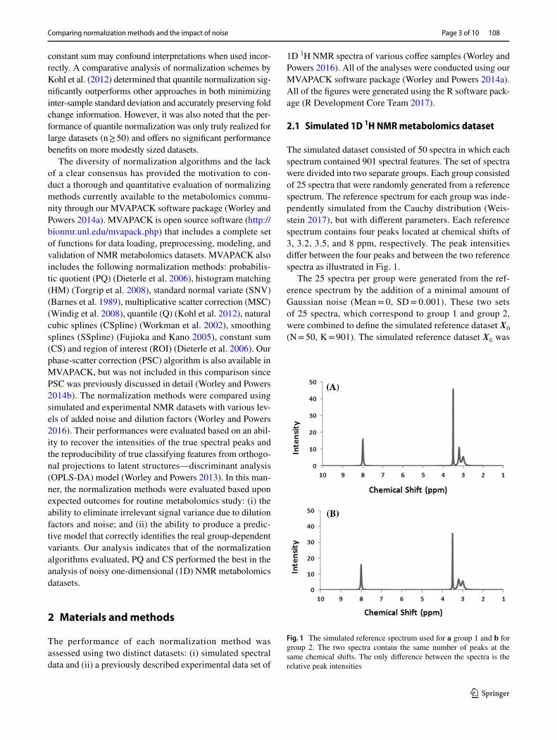
The simulated dataset consisted of 50 spectra in which each spectrum contained 901 spectral features. The set of spectra were divided into two separate groups. Each group consisted of 25 spectra that were randomly generated from a reference spectrum. The reference spectrum for each group was inde-pendently simulated from the Cauchy distribution (Weis-stein 2017), but with different parameters. Each reference spectrum contains four peaks located at chemical shifts of 3, 3.2, 3.5, and 8 ppm, respectively. The peak intensities differ between the four peaks and between the two reference spectra as illustrated in Fig. 1.

The 25 spectra per group were generated from the ref-erence spectrum by the addition of a minimal amount of Gaussian noise (Mean = 0, SD = 0.001). These two sets of 25 spectra, which correspond to group 1 and group 2, were combined to define the simulated reference dataset X0 (N = 50, K = 901). The simulated reference dataset X0 was

Fig. 1 The simulated reference spectrum used for a group 1 and b for group 2. The two spectra contain the same number of peaks at the same chemical shifts. The only difference between the spectra is the relative peak intensities

T. Vu et al.

1 3

108 Page 4 of 10

then used to generate eight noise-added simulated sets (Xi) (Fig. S1) with i = 1, 2,… , 8 (Table 1) according to Eq. (1):

where Fi is a 50 × 1 vector of dilution factors generated from a uniform distribution for the ith set, Ei is a matrix of inde-pendent Gaussian noise distributed with mean 0 and stand-ard deviation �i for the ith set, and * presents element-wise multiplication. The value of �i ranged from 0.1 to 5 which produced a systematic increase in noise for the dataset.

The CS, PQ, HM, SNV, MSC, ROI, Q, CSpline, and SSpline normalization methods were then separately applied to each noise-added set ( Xi ) to obtain normalized set ( X̃i ). An OPLS-DA model was then generated from each nor-malized set ( X̃i ). Two-component OPLS-DA models were calculated to obtain the first component loadings to compare the performance of the normalization approaches.

2.2 Experimental 1D 1H NMR metabolomics dataset

A data matrix of 32 1D 1H NMR spectra from a publicly available coffees dataset was used to further evaluate the normalization algorithms (Worley and Powers 2016). The coffees dataset contains two groups defined as light and medium decaffeinated coffee consisting of 16 1D 1H NMR spectra per group. Each spectrum contains 284 spectral features.

We applied the same procedures as described above to generate the noise-added experimental dataset. Specifically, the original coffees dataset of 32 1D 1H NMR experimental spectra was designated as the reference data set Y0 (N = 32, K = 284). The reference data set Y0 was then used to gener-ate seven simulated sets ( Yi ) with i = 1, 2,… , 7 (Table 2) according to Eq. 2:

(1)Xi = Fi ∗ (X0 + Ei)

where Fi is a 32 × 1 vector of dilution factors generated from a uniform distribution for the ith set, Ei (N = 32, K = 284) is a matrix of independent Gaussian noise distributed with mean 0 and standard deviation �i for the ith set, and * presents element-wise multiplication. The value of �i ranged from 2.3 × 10−7 to 10−5 which produced a systematic increase in noise while also mimicking the relative variance in the noise present in the coffees dataset.

2.3 Summary of normalization procedures

2.3.1 Constant sum

Each spectrum of the data matrix was divided by its own integral (Dieterle et al. 2006).

2.3.2 Probabilistic quotient

The normalization factor was the most probable quotient between the signals of the corresponding spectrum and the reference spectrum (Dieterle et al. 2006). The reference spectrum was chosen as the median spectrum of the spec-tral set. Each spectrum in the dataset was divided by this normalization factor to obtain the normalized spectrum.

2.3.3 Histogram matching

Raw spectra were log transformed prior to normaliza-tion. Similar to PQ, the target reference spectrum was the median spectrum of the dataset. Histograms for each sample spectrum and target spectrum were obtained on prespeci-fied intensity intervals. A dilution factor was then chosen to minimize the differences between each sample spectrum

(2)Yi = Fi ∗ (Y0 + Ei)Table 1 Parameters used to generate the noise-added simulated spec-tra

a A dilution factor was randomly selected from the indicated range of valuesb The value of standard deviation used to generate a Gaussian distribu-tion of noise

Set Dilution factors (F)a Standard devia-tion ( �)b

Percent added noise (%)

S1 ∼ Unif (0.9, 1.1) 0.1 5S2 ∼ Unif (0.9, 1.1) 0.2 10S3 ∼ Unif (0.8, 1.2) 0.4 20S4 ∼ Unif (0.5, 1.5) 1 50S5 ∼ Unif (0.3, 1.7) 1.4 70S6 ∼ Unif (0.1, 1.9) 1.8 90S7 ∼ Unif (0.01, 2.5) 2.5 100S8 ∼ Unif (0.001, 5) 4 200

Table 2 Parameters used to generate the noise-added coffees dataset

a A dilution factor was randomly selected from the indicated range of valuesb The value of standard deviation used to generate a Gaussian distribu-tion of noise

Set Dilution factors (F)a Standard devia-tion ( �)b

Percent added noise (%)

C1 ∼ Unif (0.9, 1.1) 2.3 × 10−7 5C2 ∼ Unif (0.8, 1.2) 4.6 × 10−7 10C3 ∼ Unif (0.5, 1.5) 9.3 × 10−7 20C4 ∼ Unif (0.3, 1.7) 2.3 × 10−6 50C5 ∼ Unif (0.1, 1.9) 5 × 10−6 100C6 ∼ Unif (0.01, 2.5) 8 × 10−6 170C7 ∼ Unif (0.001, 5) 10−5 200

Comparing normalization methods and the impact of noise

1 3

Page 5 of 10 108

histogram and the target histogram (Torgrip et al. 2008). The new normalized spectrum was generated by multiplying each original spectrum by the corresponding dilution factor.

2.3.4 Standard normal variate

Each sample spectrum in the dataset was centered prior to normalization. The standard deviation of each spectrum was calculated as a normalization factor (Barnes et al. 1989). A new normalized dataset was then obtained by dividing each original spectrum by its corresponding normalization factor.

2.3.5 Multiplicative scatter correction

The normalization factors were least squares estimates obtained by regressing each sample spectrum onto the ref-erence spectrum (Windig et al. 2008). The reference spec-trum was the mean spectrum. The ordinary least squares of the regression parameters were used to correct the spectral intensities.

2.3.6 Region of interest

Each sample spectrum of the dataset was normalized to a specified spectral region where its integral was set to one. Each sample spectrum was then normalized relative to the most intense peak in the spectrum.

2.3.7 Quantile

The goal of this quantile normalization method was to obtain an identical distribution of intensities for all of the spectral features (Kohl et al. 2012). First, the mean spectrum was cal-culated for the data set. The intensities of all features in each sample spectrum were then replaced by the mean intensities in accordance with their quantile orders.

2.3.8 Natural cubic splines

The CSpline method normalized each sample spectrum to the target spectrum. The target spectrum was calcu-lated using the non-linear arithmetic mean of the data set. Depending on the type of data, a geometric mean may also be used (Kohl et al. 2012). A set of 100 quantiles was taken from both the sample spectrum and the target spectrum. The quantiles were then fitted to a natural cubic spline to obtain parameter estimates, which were used for interpolations. The process was repeated five times. For each iteration, a small offset was added to the quantiles before refitting with a natural cubic spline to obtain new interpolations. The set of interpolations were averaged to obtain the normalized spectrum.

2.3.9 Smoothing splines

SSpline is similar to CSpline, but the SSpline algorithm adds more quantiles toward the tail end of the spectrum. The most intense spectral features are located in this region of the spectrum. Moreover, the quantiles are fitted with a smoothing spline that includes a penalty parameter to avoid overfitting. The predicted feature intensities were then used as the normalized intensities.

2.4 Evaluation criteria

Regardless of the type of approach used to address dataset bias or variance, an optimal normalization procedure should reduce any unwanted noise while still preserving the true biological signals. In other words, a necessary condition to retain the true signals is the ability to recover the origi-nal peak intensities after removing noise. In this regards, it should be possible to evaluate the relative performance of normalization methods based on how well the algorithms handle increasingly noisy spectra. As the reference set is exposed to increasing amounts of noise, some (or all) of the normalization algorithms would be expected to fail to recover the original peaks intensities. Thus, the peak recov-ery criteria served as a means to filter-out poorly perform-ing normalization procedures prior to proceeding with the second evaluation criteria.

A multivariate statistical model, such as PCA or OPLS, is typically employed to identify spectral features that sepa-rate the different groups in the dataset (Worley and Powers 2013). These spectral features are intrinsic to the dataset. Accordingly, any properly normalized dataset should repro-duce these true set of features. The first component loadings extracted from an OPLS-DA model contains the weights of the spectral features that contribute the most to separating the groups. Simply, the first component loadings identify the most-important group-dependent features. Thus, an OPLS-DA model was generated to obtain the first component load-ings associated with each normalization method. Only the top performing normalization methods were used to gener-ate an OPLS-DA model. The top performing normalization methods were identified based on the peak recovery criteria. Pearson correlation coefficients were calculated between the loadings of each normalized dataset and the true loadings set. The Pearson correlation coefficients provide a means to measure the reproducibility of the true classifying spectral features produced by each normalization algorithm.

2.4.1 Peak recovery

After sequentially normalizing each noisy data matrix using the nine normalization methods, the intensity of each peak in each spectrum of the normalized set ( X̃i ) was compared

T. Vu et al.

1 3

108 Page 6 of 10

to the true original spectrum ( X0 ) to measure the recovery of peak intensities ( rpij

i ). For each spectrum from the nor-

malized data matrix ( X̃i ), the recovery of the jth peak was calculated according to this Eq. 3:

where Iji and Ij

0 are the intensities of the jth peak from X̃i

and X0 , respectively. In this manner, rpiji will range from

0 to 1 regardless of the relative magnitudes of Iji and Ij

0 .

This process was repeated for every peak in each spectrum. The mean recovery and standard error were calculated and reported for each normalized set.

2.4.2 Pearson correlation coefficients

The coffees noisy data matrix ( Yi ) was only normalized using the top performing algorithms identified from the peak recovery criteria. An OPLS-DA model was generated for each normalized coffees data matrix ( ̃Yi ) and also the original coffees data set ( Yo ). The datasets were scaled with Pareto scaling prior to calculating the OPLS-DA models. The first component loadings from each OPLS-DA model were then used to calculate a Pearson correlation coefficient between the true backscale loadings vector ( po ) from the original coffees data set ( Yo ) and the backscale loadings vector ( pi ) from each normalized coffees noisy data matric ( ̃Yi ). The Pearson correlation coefficients were calculated according to Eq. 4:

where K denotes the number of spectral features; p̄i is the mean loading of vector pi ; pki is the kth loading of vector pi ; p̄0 is the mean loading of vector p0 ; and pk

0 is the kth loading

of vector p0 . This process was repeated 100 times. The mean correlation coefficients and standard error were calculated for each normalized set.

3 Results and discussion

The two reference NMR spectra displayed in Fig. 1 were used to generate eight noise-added simulated metabolomics datasets consisting of 25 spectra for each of the two groups (Fig. S1). Accordingly, each simulated dataset contained a total of 50 spectra. The total signal variance in each dataset was defined by the amount of Gaussian noise added and by

(3)rpij

i=

⎛⎜⎜⎜⎝1 −

���Ij

i− I

j

0

���max

����Ij

0

���,���I

j

i

����⎞⎟⎟⎟⎠

(4)ri =

∑K

k=1(pk

i− p̄i)(p

k0− p̄0)�∑K

k=1

�pki− p̄i

�2 ∑K

k=1

�pk0− p̄0

�2

the dilution factors listed in Table 1. The simulated NMR metabolomics datasets were then normalized using each of the nine normalization methods (i.e., CS, CSpline, HM, MSC, PQ, Q, ROI, SNV, and SSpline). A peak recovery was calculated for each dataset according to Eq. 3. The peak recovery compares each of the normalized dataset to the original reference NMR spectra (Fig. 1). The peak recover-ies for each normalized dataset are plotted in Figs. 2 and 3.

As expected, the efficiency of peak recovery decreases with increasing signal variance regardless of the normaliza-tion method. As illustrated in Fig. 2, most of the normaliza-tion methods achieve nearly 100% peak recovery (96 to 99%) under conditions of modest signal variance (S1 and S2).

The most notable outlier is HM, which achieved a peak recovery of only 20–28%. This extremely poor performance suggests that HM should be avoided and not used for the normalization of NMR metabolomics data. While signifi-cantly better than HM, SSpline also performed consistently below average with a peak recovery range of 93–95%. PQ was modestly below the best performers with a peak recov-ery range of 96–97%. Conversely, ROI, CS, SNV, MSC, and Q, recovered at least 98% of the peak intensities under conditions of modest signal variance. A further separation in algorithm performance was apparent as the signal vari-ance was progressively increased. SSpline continued to per-form worse than average, but from simulated set S5 forward the performance of SNV had also significantly declined to match SSpline.

Similarly, from simulated set S6, CSpline had fallen below the average performance of the other normalization

Fig. 2 A plot of the recovery of peak intensities (Eq. 3) for the 9 nor-malization methods after being applied to the 8 (S1 to S8) simulated datasets listed in Table 1. The total signal variance due to the amount of added Gaussian noise and the magnitude of the dilution factor increases from S1 to S8. The horizontal dashed lines represent a full recovery at 100% and partial recovery at 50%. Each bar represents the mean peak recovery and the error bars represent ± 2 * standard error of the mean

Comparing normalization methods and the impact of noise

1 3

Page 7 of 10 108

methods. In fact, as the amount of signal variance was increased to the highest level (S8), the peak recoveries for CSpline, HM, MSC, Q, and SSpline all fell below 50%. Conversely, CS, PQ and ROI maintained a peak recovery of around 70% (67–74%). Accordingly, the peak recovery results suggest that the CS, PQ and ROI were the most robust normalization methods and were able to maintain a maximal peak recovery as a function of signal variance (Fig. 3). Pairwise Student’s t tests of the mean peak recov-ery values at the highest signal variance level (S8) yield a maximum p-value of < 2.8 × 10−13 between the CS, PQ, ROI algorithms and the other normalization methods.

To further investigate the individual impact of Gaussian noise and dilution factors on peak recovery, the simulation was repeated for the three top performing normalization methods (i.e., CS, PQ and ROI). Instead of simultaneously varying both Gaussian noise and the dilution factors as listed in Table 1, the simulation was repeated with either Gauss-ian noise or the dilution factor held constant at S1 values. The combined average peak recovery values for CS, PQ and ROI normalized datasets are plotted as a function of added Gaussian noise or dilution factor in Fig. 4. This simulation yielded an unexpected result. The performance of the nor-malization method was essentially unaffected by the dilution factor. Near perfect peak recovery was obtained even for the highest dilution factor. Instead, the normalization perfor-mance was strictly dependent on the level of Gaussian noise added to the spectra. However, it is important to note that normalization methods also rely on good peak alignment,

spectral phasing, baseline correction and solvent suppres-sion in order to perform well. Accordingly, the simulations reported herein were restricted to well-behaved datasets.

While being able to accurately reconstitute peak intensity is an important attribute of a normalization algorithm, the proper identification of group-defining spectral features is still a vital necessity. In essence, are biologically-relevant metabolic differences still being correctly identified regard-less of the natural signal variance? Does a PCA or OPLS scores plot yield statistically relevant group separations and do the loadings identify the “true” metabolic differences between the groups? To address this issue, the CS, PQ and ROI normalization methods were further evaluated based on the reproducibility of OPLS-DA models as a function of increasing signal variance. An experimental coffees dataset previously used to investigate PCA and OPLS model stabil-ity (Worley and Powers 2016), was employed to generate OPLS-DA models using the CS, PQ and ROI normaliza-tion methods. Specifically, the coffee dataset consists of 32 1D 1H NMR spectra for two groups of observations (light and medium decaffeinated coffees). The coffees dataset was modified with Gaussian noise and a dilution factor (Fig. S2) as outlined in Table 2. Consistent with our prior obser-vations (Worley and Powers 2016), the two coffee groups become indistinguishable with an increase in signal vari-ance. Importantly, the estimated loadings from the corre-sponding OPLS-DA model are less correlated to the true loadings (Fig. 5) with increasing signal variance. Notably, at minimal to moderate signal variance levels (C1 to C3), the

Fig. 3 A plot of the recovery of peak intensities (Eq. 3) for the three top performing normalization methods after being applied to the 8 (S1 to S8) simulated datasets listed in Table 1. The total signal vari-ance due to the amount of added Gaussian noise and the magnitude of the dilution factor increases from S1 to S8. The horizontal dashed lines represent a full recovery at 100% and partial recovery at 50%. Each bar represents the mean peak recover and the error bars repre-sent ± 2 * standard error of the mean

0.6

0.7

0.8

0.9

1

S1 S2 S3 S4 S5 S6 S7 S8

Peak

Rec

over

y

Simulated Set

Fig. 4 A plot of the average peak recovery calculated from the three top-performing normalization methods (CS, PQ, and ROI). Datasets were regenerated according to the scheme described in Table  1 but containing only a dilution factor (filled diamond) or the addition of Gaussian noise (filled square). The dilution factor or added Gaussian noise was held constant at S1 values when the other parameter was varied. The peak recovery decreases with additive noise, but is unaf-fected by dilution factor

T. Vu et al.

1 3

108 Page 8 of 10

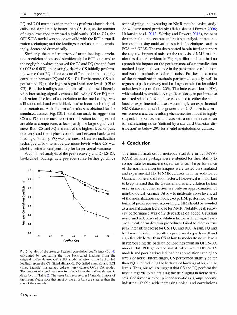
PQ and ROI normalization methods perform almost identi-cally and significantly better than CS. But, as the amount of signal variance increased significantly (C4 to C7), the OPLS-DA model was no longer valid with the ROI normali-zation technique; and the loadings correlation, not surpris-ingly, decreased dramatically.

Similarly, the standard errors of mean loadings correla-tion coefficients increased significantly for ROI compared to the negligible values observed for CS and PQ (ranged from 0.0003 to 0.008). Interestingly, despite CS initially perform-ing worse than PQ, there was no difference in the loadings correlation between PQ and CS at C4. Furthermore, CS out-performed PQ at the highest signal variance levels (C5 to C7). But, the loadings correlations still decreased linearly with increasing signal variance following CS or PQ nor-malization. The loss of a correlation to the true loadings was still substantial and would likely lead to incorrect biological interpretations. A similar set of results was obtained for the simulated dataset (Fig. S3). In total, our analysis suggest that CS and PQ are the most robust normalization techniques and are able to compensate, at least partly, for large signal vari-ance. Both CS and PQ maintained the highest level of peak recovery and the highest correlation between backscaled loadings. Notably, PQ was the most robust normalization technique at low to moderate noise levels while CS was slightly better at compensating for larger signal variance.

A combined analysis of the peak recovery and OPLS-DA backscaled loadings data provides some further guidance

for designing and executing an NMR metabolomics study. As we have noted previously (Halouska and Powers 2006; Halouska et al. 2013; Worley and Powers 2016), noise is detrimental to the accurate and reliable analysis of metabo-lomics data using multivariate statistical techniques such as PCA and OPLS. The results reported herein further support the negative impact of noise on the analysis of NMR metab-olomics data. As evident in Fig. 4, a dilution factor had no appreciable impact on the performance of a normalization method. Instead, all variance in the performance of the nor-malization methods was due to noise. Furthermore, most of the normalization methods performed equally-well in regards to peak recovery and loadings correlation for added noise levels up to about 20%. The lone exception is HM, which should be avoided. A significant decay in performance occurred when > 20% of noise was added to either the simu-lated or experimental dataset. Accordingly, an experimental NMR dataset that exhibits greater than 20% noise is a seri-ous concern and the resulting chemometrics model is highly suspect. In essence, our analysis sets a minimum criterion for maintaining noise (defined by a standard Gaussian dis-tribution) at below 20% for a valid metabolomics dataset.

4 Conclusion

The nine normalization methods available in our MVA-PACK software package were evaluated for their ability to compensate for increasing signal variance. The performance of the normalization techniques were tested on simulated and experimental 1D 1H NMR datasets with the addition of Gaussian noise and dilution factors. However, it is important to keep in mind that the Gaussian noise and dilution factors used in model construction are only an approximation of non-biological variance. At low to moderate noise levels, all of the normalization methods, except HM, performed well in terms of peak recovery. Accordingly, HM should be avoided as a normalization technique for NMR. Notably, peak recov-ery performance was only dependent on added Gaussian noise, and independent of dilution factor. At high signal vari-ance, most normalization procedures failed to recover true peak intensities except for CS, PQ, and ROI. Again, PQ and ROI normalization algorithms performed equally-well and significantly better than CS at low to moderate noise levels in reproducing the backscaled loadings from an OPLS-DA model. But, ROI generated statistically invalid OPLS-DA models and poor backscaled loadings correlations at higher-levels of noise. Interestingly, CS performed slightly better than PQ in reproducing the backscaled loadings at high noise levels. Thus, our results suggest that CS and PQ perform the best in regards to maintaining the true signal in noisy data-sets. Consistent with our prior observations, groups become indistinguishable with increasing noise; and correlations

-0.4

-0.2

0.0

0.2

0.4

0.6

0.8

1.0

C1 C2 C3 C4 C5 C6 C7

Pear

son

Corr

ela

on C

oeffi

cien

ts

Coffee Set

Fig. 5 A plot of the average Pearson correlation coefficients (Eq. 4) calculated by comparing the true backscaled loadings from the original coffee dataset OPLS-DA model relative to the backscaled loadings from the CS (filled diamond), PQ (filled square), and ROI (filled triangle) normalized coffees noisy dataset OPLS-DA model. The amount of signal variance introduced into the coffees dataset is described in Table 2. The error bars represent ± 2 * standard error of the mean. Please note that most of the error bars are smaller than the size of the symbols

Comparing normalization methods and the impact of noise

1 3

Page 9 of 10 108

to the true loadings are lost. In other words, an increasing level of additive Gaussian noise masks the true signals in the datasets. Accordingly, if this noise is not handled properly, it will lead to false conclusions and biologically irrelevant observations. In this regards, our analysis suggests that, at a minimum, noise needs to remain below 20% in order for an NMR metabolomics dataset to provide an accurate and biologically-relevant chemometrics model.

Acknowledgements We thank Dr. Martha Morton, the Director of the Research Instrumentation Facility in the Department of Chem-istry at the University of Nebraska-Lincoln for her assistance with the NMR experiments. This material is based upon work supported by the National Science Foundation under Grant Number (1660921). This work was supported in part by funding from the Redox Biology Center (P30 GM103335, NIGMS); and the Nebraska Center for Inte-grated Biomolecular Communication (P20 GM113126, NIGMS). The research was performed in facilities renovated with support from the National Institutes of Health (RR015468-01). Any opinions, findings, and conclusions or recommendations expressed in this material are those of the author(s) and do not necessarily reflect the views of the National Science Foundation.

Author contributions TV and ER performed the experiments; RP and YQ designed the experiments; TV, ER, YQ, and RP analyzed the data and wrote the manuscript.

Compliance with ethical standards

Conflict of interest Authors have no conflict of interest to declare.

Ethical approval This article does not contain any studies with human participants or animals performed by any of the authors.

References

Aardema, M. J., & MacGregor, J. T. (2002). Toxicology and genetic toxicology in the new era of “toxicogenomics”: Impact of “-omics” technologies. Mutation Research/Fundamental and Molecular Mechanisms of Mutagenesis, 499, 13–25. https ://doi.org/10.1016/S0027 -5107(01)00292 -5.

Barnes, R. J., Dhanda, M. S., & Lister, S. J. (1989). Standard normal variate transformation and de-trending of near-infrared diffuse reflectance spectra. Applied Spectroscopy, 43, 772–777.

Berger, B., Peng, J., & Singh, M. (2013). Computational solutions for omics data. Nature Reviews Genetics, 14, 333–346. https ://doi.org/10.1038/nrg34 33.

Butcher, E. C., Berg, E. L., & Kunkel, E. J. (2004). Systems biology in drug discovery. Nature Biotechnology, 22, 1253. https ://doi.org/10.1038/nbt10 17.

Callister, S. J., Barry, R. C., Adkins, J. N., Johnson, E. T., Qian, W. J., Webb-Robertson, B. J. M., … Lipton, M. S. (2006). Normaliza-tion approaches for removing systematic biases associated with mass spectrometry and label-free proteomics. Journal of Pro-teome Research, 5, 277–286. https ://doi.org/10.1021/pr050 300l.

Chawade, A., Alexandersson, E., & Levander, F. (2014). Normalyzer: A tool for rapid evaluation of normalization methods for omics data sets. Journal of Proteome Research, 13, 3114–3120. https ://doi.org/10.1021/pr401 264n.

Chen, R., Mias, G. I., Li-Pook-Than, J., Jiang, L., Lam, H. Y., Chen, R., … Cheng, Y. (2012). Personal omics profiling reveals dynamic molecular and medical phenotypes. Cell, 148, 1293–1307. https ://doi.org/10.1016/j.cell.2012.02.009.

Choe, S. E., Boutros, M., Michelson, A. M., Church, G. M., & Halfon, M. S. (2005). Preferred analysis methods for Affy-metrix GeneChips revealed by a wholly defined control dataset. Genome Biology, 6, R16. https ://doi.org/10.1186/gb-2005-6-2-r16.

Craig, A., Cloarec, O., Holmes, E., Nicholson, J. K., & Lindon, J. C. (2006). Scaling and normalization effects in NMR spectroscopic metabonomic data sets. Analytical Chemistry, 78, 2262–2267. https ://doi.org/10.1021/ac051 9312.

Cuykx, M., Claes, L., Rodrigues, R. M., Vanhaecke, T., & Covaci, A. (2018). Metabolomics profiling of steatosis progression in HepaRG® cells using sodium valproate. Toxicology Letters, 286, 22–30. https ://doi.org/10.1016/j.toxle t.2017.12.015.

Dieterle, F., Ross, A., Schlotterbeck, G., & Senn, H. (2006). Proba-bilistic quotient normalization as robust method to account for dilution of complex biological mixtures. Application in 1H NMR metabonomics. Analytical Chemistry, 78, 4281–4290. https ://doi.org/10.1021/ac051 632c.

Doran, M. L., Knee, J. M., Wang, N., Rzezniczak, T. Z., Parkes, T. L., Li, L., & Merritt, T. J. (2017). Metabolomic analysis of oxida-tive stress: Superoxide dismutase mutation and paraquat induced stress in Drosophila melanogaster. Free Radical Biology and Medicine, 113, 323–334. https ://doi.org/10.1016/j.freer adbio med.2017.10.011.

Fujioka, H., & Kano, H. (2005). Smoothing spline curves and surfaces for sampled data. International Journal of Innovative Computing, 1, 429–449.

Fukushima, A., Iwasa, M., Nakabayashi, R., Kobayashi, M., Nishizawa, T., Okazaki, Y., … Kusano, M. (2017). Effects of combined low glutathione with mild oxidative and low phosphorus stress on the metabolism of Arabidopsis thaliana. Frontiers in Plant Science, 8, 1464.

Giraudeau, P., Tea, I., Remaud, G. S., & Akoka, S. (2014). Reference and normalization methods: Essential tools for the intercompari-son of NMR spectra. Journal of Pharmaceutical and Biomedical Analysis, 93, 3–16. https ://doi.org/10.1016/j.jpba.2013.07.020.

Halouska, S., Zhang, B., Gaupp, R., Lei, S., Snell, E., Fenton, R. J., ... Powers, R. (2013). Revisiting protocols for the NMR analysis of bacterial metabolomes. Journal of Integrated OMICS, 2, 120–137.

Halouska, S., & Powers, R. (2006). Negative impact of noise on the principal component analysis of NMR data. Journal of Magnetic Resonance, 178, 88–95.

Hochrein, J., Zacharias, H. U., Taruttis, F., Samol, C., Engelmann, J. C., Spang, R., … Gronwald, W. (2015). Data normalization of 1H NMR metabolite fingerprinting data sets in the presence of unbalanced metabolite regulation. Journal of Proteome Research, 14, 3217–3228. https ://doi.org/10.1021/acs.jprot eome.5b001 92.

Jung, Y.-S., Lee, J., Seo, J., & Hwang, G.-S. (2017). Metabolite profil-ing study on the toxicological effects of polybrominated diphenyl ether in a rat model. Environmental Toxicology, 32, 1262–1272. https ://doi.org/10.1002/tox.22322 .

Kohl, S. M., Klein, M. S., Hochrein, J., Oefner, P. J., Spang, R., & Gronwald, W. (2012). State-of-the art data normalization meth-ods improve NMR-based metabolomic analysis. Metabolomics, 8, 146–160. https ://doi.org/10.1007/s1130 6-011-0350-z.

R Development Core Team. (2017). R: A language and environment for statistical computing. Austria: R Foundation for Statistical Computing Vienna.

Thulin, E., Thulin, M., & Andersson, D. I. (2017). Reversion of high-level mecillinam resistance to susceptibility in Escherichia coli during growth in urine. EBioMedicine, 23, 111–118. https ://doi.org/10.1016/j.ebiom .2017.08.021.

T. Vu et al.

1 3

108 Page 10 of 10

Torgrip, R. J. O., Åberg, K. M., Alm, E., Schuppe-Koistinen, I., & Lindberg, J. (2008). A note on normalization of biofluid 1D 1H-NMR data. Metabolomics, 4, 114–121. https ://doi.org/10.1007/s1130 6-007-0102-2.

Weisstein, E. W. (2017). Cauchy distribution. In: MathWorld. http://mathw orld.wolfr am.com/Cauch yDist ribut ion.html.

Windig, W., Shaver, J., & Bro, R. (2008). Loopy MSC: A simple way to improve multiplicative scatter correction. Applied Spectroscopy, 62, 1153–1159. https ://doi.org/10.1366/00037 02087 86049 097.

Wishart, D. S. (2008). Metabolomics: Applications to food science and nutrition research. Trends in Food Science & Technology, 19, 482–493. https ://doi.org/10.1016/j.tifs.2008.03.003.

Workman, C., Jensen, L. J., Jarmer, H., Berka, R., Gautier, L., Nielser, H. B., … Knudsen, S. (2002). A new non-linear normalization method for reducing variability in DNA microarray experiments. Genome Biology. https ://doi.org/10.1186/gb-2002-3-9-resea rch00 48.

Worley, B., & Powers, R. (2013). Multivariate analysis in metabo-lomics. Current Metabolomics, 1, 92–107. https ://doi.org/10.2174/22132 35X11 30101 0092.

Worley, B., & Powers, R. (2014a). MVAPACK: A complete data han-dling package for NMR metabolomics. ACS Chemical Biology, 9, 1138–1144. https ://doi.org/10.1021/cb400 8937.

Worley, B., & Powers, R. (2014b). Simultaneous phase and scatter correction for NMR datasets. Chemometrics and Intelligent Laboratory Systems, 131, 1–6. https ://doi.org/10.1016/j.chemo lab.2013.11.005.

Worley, B., & Powers, R. (2016). PCA as a practical indicator of OPLS-DA model reliability. Current Metabolomics, 4, 97–103. https ://doi.org/10.2174/22132 35x04 66616 06131 22429 .

Zyprych-Walczak, J., Szabelska, A., Handschuh, L., Górc-zak, K., Klamecka, K., Figlerowicz, M., & Siatkowski, I. (2015). The impact of normalization methods on RNA-Seq data analysis. BioMed Research International. https ://doi.org/10.1155/2015/62169 0.