
Comparing Deep Reinforcement Learning Methods for ...und...Reinforcement Learning methods (Deep...
140
Otto-von-Guericke-Universit¨ at Magdeburg Faculty of Computer Science Master’s Thesis Comparing Deep Reinforcement Learning Methods for Engineering Applications Author: Shengnan Chen August 25, 2018 Advisors: Prof. Dr.-Ing. habil. Sanaz Mostaghim Intelligent Cooperating Systems (IKS) M.Sc. Gabriel Campero Durand Technical and Operational Information Systems (ITI)
Transcript of Comparing Deep Reinforcement Learning Methods for ...und...Reinforcement Learning methods (Deep...

Otto-von-Guericke-Universitat Magdeburg
Faculty of Computer Science
Master’s Thesis
Comparing Deep ReinforcementLearning Methods for Engineering
Applications
Author:
Shengnan Chen
August 25, 2018
Advisors:
Prof. Dr.-Ing. habil. Sanaz Mostaghim
Intelligent Cooperating Systems (IKS)
M.Sc. Gabriel Campero Durand
Technical and Operational Information Systems (ITI)

Chen, Shengnan:Comparing Deep Reinforcement Learning Methods for Engineering ApplicationsMaster’s Thesis, Otto-von-Guericke-Universitat Magdeburg, 2018.

Abstract
In recent years the field of Reinforcement Learning has come across a series of break-throughs. By combining with developments from working with complex neural networks,popularly called Deep Learning, practitioners have started proposing various Deep Rein-forcement Learning (DRL) solutions, which are capable of learning complex tasks whilekeeping a limited representation of the information learned. Nowadays, researchers havestarted applying such methods to different kinds of applications, seeking to exploit theability of this learning approach to improve with experience. However, the DRL methodsproposed in this recent period are still under development, as a result researchers in thefield face several practical challenges in determining which methods are applicable totheir use cases, and which specific design and runtime characteristics of the methodsdemand consideration for optimal applications.
In this Thesis we study the requirements expected from DRL in engineering applications,and we evaluate to which extent these can be addressed through specific configurationsof the DRL methods. To this end we implement different agents using three DeepReinforcement Learning methods (Deep Q-Learning, Deep Deterministic Policy Gra-dient and Distributed Proximal Policy Optimization); to solve tasks on three differentenvironments (CartPole, PlaneBall, and CirTurtleBot), intended to represent mechanicaland strategical tasks. Through our evaluation we are able to report characteristics ofthe methods studied. Our results can support decision making for ranking the threemethods according to their suitability to given specific application requirements. Weexpect that our evaluation approach can also contribute to showing how comparisonacross models could be carried out, providing researchers with the information theyneed about methods.

Acknowledgements
First and foremost, I am grateful to my advisor M.Sc. Gabriel Campero Durand for hisguidance, patience and constant encouragement without which this may not have beenpossible.
I would like to thank Prof. Dr. Sanaz Mostaghim for giving me the opportunity to writemy Master’s thesis at her chair.
I would like to thank Dr.-Ing. Akos Csiszar in Stuttgart University for providing methis topic.
It has been a privilege for me to work in field of reinforcement learning.
I would like to thank my family and friends, who supported me in completing my studiesand in writing my thesis.

Declaration of Academic Integrity
I hereby declare that this thesis is solely my own work and I have cited all externalsources used.
Magdeburg, August 25th 2018
———————–Shengnan Chen

Contents
List of Figures xi
1 Introduction 11.1 Context for our work . . . . . . . . . . . . . . . . . . . . . . . . . . . . . 1
1.1.1 Artificial intelligence and its relevance to industry . . . . . . . . . 11.1.2 Reinforcement learning and deep reinforcement learning . . . . . . 31.1.3 RL for engineering applications and its challenges . . . . . . . . . 41.1.4 The need for benchmarks for RL in engineering applications . . . 5
1.2 Problem statement . . . . . . . . . . . . . . . . . . . . . . . . . . . . . . 61.3 Research aim . . . . . . . . . . . . . . . . . . . . . . . . . . . . . . . . . 71.4 Research methodology . . . . . . . . . . . . . . . . . . . . . . . . . . . . 71.5 Thesis structure . . . . . . . . . . . . . . . . . . . . . . . . . . . . . . . . 9
2 Background: Reinforcement learning and deep reinforcement learn-ing 102.1 Reinforcement learning . . . . . . . . . . . . . . . . . . . . . . . . . . . . 10
2.1.1 Q learning . . . . . . . . . . . . . . . . . . . . . . . . . . . . . . . 172.1.2 Policy gradient . . . . . . . . . . . . . . . . . . . . . . . . . . . . 172.1.3 Limitations of RL in practice . . . . . . . . . . . . . . . . . . . . 21
2.2 Deep learning . . . . . . . . . . . . . . . . . . . . . . . . . . . . . . . . . 232.2.1 Convolution Neural Network(CNN) . . . . . . . . . . . . . . . . . 252.2.2 Recurrent Neural Network(RNN) . . . . . . . . . . . . . . . . . . 282.2.3 Hyperparameters . . . . . . . . . . . . . . . . . . . . . . . . . . . 29
2.3 Deep Reinforcement Learning . . . . . . . . . . . . . . . . . . . . . . . . 312.3.1 Overview . . . . . . . . . . . . . . . . . . . . . . . . . . . . . . . 312.3.2 Deep Q Network . . . . . . . . . . . . . . . . . . . . . . . . . . . 312.3.3 Deep Deterministic Policy Gradient . . . . . . . . . . . . . . . . . 352.3.4 Proximal Policy Optimization . . . . . . . . . . . . . . . . . . . . 372.3.5 Asynchronous Advanced Actor Critic . . . . . . . . . . . . . . . . 40
2.4 Summary . . . . . . . . . . . . . . . . . . . . . . . . . . . . . . . . . . . 41
3 Background: Deep reinforcement learning for engineering applications43
3.1 Reinforcement Learning for Engineering Applications . . . . . . . . . . . 43

Contents vii
3.1.1 Engineering Applications . . . . . . . . . . . . . . . . . . . . . . . 433.1.1.1 Categories for Engineering Applications . . . . . . . . . 443.1.1.2 Applications of Artificial Intelligence in Engineering . . . 44
3.1.2 What is the Role of RL in Engineering Applications? . . . . . . . 453.1.2.1 Building an optimize the product inventory system . . . 463.1.2.2 Building HVAC control system . . . . . . . . . . . . . . 463.1.2.3 Building an intelligent plant monitoring and predictive
maintenance system . . . . . . . . . . . . . . . . . . . . 463.1.3 Characteristics of RL in Engineering Applications . . . . . . . . . 473.1.4 RL Life Cycle in Engineering Applications . . . . . . . . . . . . . 483.1.5 Challenges in RL for Engineering Applications . . . . . . . . . . . 49
3.1.5.1 RL algorithms limits and high requirements of policiesimprovement . . . . . . . . . . . . . . . . . . . . . . . . 49
3.1.5.2 Physical world uncertainty . . . . . . . . . . . . . . . . . 493.1.5.3 Simulation environment . . . . . . . . . . . . . . . . . . 503.1.5.4 Reward function design . . . . . . . . . . . . . . . . . . 513.1.5.5 Professional knowledge requirements . . . . . . . . . . . 51
3.2 Challenges in Deep RL for Engineering Applications . . . . . . . . . . . . 523.2.1 Lack of use cases . . . . . . . . . . . . . . . . . . . . . . . . . . . 523.2.2 The need for comparisons . . . . . . . . . . . . . . . . . . . . . . 523.2.3 Lack of standard benchmarks . . . . . . . . . . . . . . . . . . . . 52
3.3 Summary . . . . . . . . . . . . . . . . . . . . . . . . . . . . . . . . . . . 52
4 Prototypical implementation and research questions 544.1 Research Questions . . . . . . . . . . . . . . . . . . . . . . . . . . . . . . 544.2 Tools . . . . . . . . . . . . . . . . . . . . . . . . . . . . . . . . . . . . . . 554.3 Environments . . . . . . . . . . . . . . . . . . . . . . . . . . . . . . . . . 59
4.3.1 CartPole . . . . . . . . . . . . . . . . . . . . . . . . . . . . . . . . 604.3.2 PlaneBall . . . . . . . . . . . . . . . . . . . . . . . . . . . . . . . 614.3.3 CirTurtleBot . . . . . . . . . . . . . . . . . . . . . . . . . . . . . 63
4.4 Experimental Setting . . . . . . . . . . . . . . . . . . . . . . . . . . . . . 654.5 Summary . . . . . . . . . . . . . . . . . . . . . . . . . . . . . . . . . . . 65
5 Evaluation and results 665.1 “One-by-One” performance Comparison . . . . . . . . . . . . . . . . . . . 66
5.1.1 DQN method in the environments . . . . . . . . . . . . . . . . . . 675.1.2 DDPG method in the environments . . . . . . . . . . . . . . . . . 815.1.3 PPO method in the environments . . . . . . . . . . . . . . . . . . 93
5.2 Methods comparison through environments . . . . . . . . . . . . . . . . . 1045.2.1 Comparison in “CartPole” . . . . . . . . . . . . . . . . . . . . . . 1065.2.2 Comparison in “PlaneBall” . . . . . . . . . . . . . . . . . . . . . . 1085.2.3 Comparison in “CirTurtleBot” . . . . . . . . . . . . . . . . . . . . 110
5.3 Summary . . . . . . . . . . . . . . . . . . . . . . . . . . . . . . . . . . . 112

viii Contents
6 Related work 1136.0.1 Engineering Applications . . . . . . . . . . . . . . . . . . . . . . . 1136.0.2 Challenges of RL in Engineering Applications . . . . . . . . . . . 1146.0.3 Benchmarks for RL . . . . . . . . . . . . . . . . . . . . . . . . . . 115
6.1 Summary . . . . . . . . . . . . . . . . . . . . . . . . . . . . . . . . . . . 116
7 Conclusions and future work 1177.1 Work summary . . . . . . . . . . . . . . . . . . . . . . . . . . . . . . . . 1177.2 Threats to validity . . . . . . . . . . . . . . . . . . . . . . . . . . . . . . 1187.3 Future work . . . . . . . . . . . . . . . . . . . . . . . . . . . . . . . . . . 119
Bibliography 120

List of Figures
1.1 Machine learning types1 . . . . . . . . . . . . . . . . . . . . . . . . . . . 2
1.2 CRISP-DM process model 2 . . . . . . . . . . . . . . . . . . . . . . . . . 9
2.1 The basic reinforcement learning model 3 . . . . . . . . . . . . . . . . . . 11
2.2 Category of Reinforcement learning methods . . . . . . . . . . . . . . . . 16
2.3 Policy Gradient methods . . . . . . . . . . . . . . . . . . . . . . . . . . . 20
2.4 Actor-Critic Architecture 4 . . . . . . . . . . . . . . . . . . . . . . . . . . 22
2.5 Simple NNs and Deep NNs 5 . . . . . . . . . . . . . . . . . . . . . . . . . 24
2.6 Architecture of LeNet-5 [LBBH98] . . . . . . . . . . . . . . . . . . . . . . 26
2.7 Architecture of AlexNet [KSH12] . . . . . . . . . . . . . . . . . . . . . . 26
2.8 Summary table of popular CNN architectures 6 . . . . . . . . . . . . . . 27
2.9 Typical RNN structure 7 . . . . . . . . . . . . . . . . . . . . . . . . . . . 28
2.10 Deep Q-learning structure 8 . . . . . . . . . . . . . . . . . . . . . . . . . 33
2.11 Deep Q-learning with Experience Replay [MKS+13] . . . . . . . . . . . . 34
2.12 DDPG Pseudocode [LHP+15] . . . . . . . . . . . . . . . . . . . . . . . . 36
2.13 PPO Pseudocode by OpenAI [SWD+17] . . . . . . . . . . . . . . . . . . 39
2.14 PPO Pseudocode by DeepMind [HSL+17] . . . . . . . . . . . . . . . . . . 39
2.15 A3C procedure 9 . . . . . . . . . . . . . . . . . . . . . . . . . . . . . . . 40
2.16 A3C Neural network structure 10 . . . . . . . . . . . . . . . . . . . . . . 41
2.17 A3C Pseudocode [MBM+16] . . . . . . . . . . . . . . . . . . . . . . . . . 42
3.1 RL in engineering applications 11 . . . . . . . . . . . . . . . . . . . . . . 47
4.1 Gym code snippet [BCP+16] . . . . . . . . . . . . . . . . . . . . . . . . . 56

x List of Figures
4.2 Toolkit for RL in robotics [ZLVC16] . . . . . . . . . . . . . . . . . . . . . 57
4.3 CartPole-v0 12 . . . . . . . . . . . . . . . . . . . . . . . . . . . . . . . . . 61
4.4 Observations and Actions in CartPole-v0 13 . . . . . . . . . . . . . . . . 62
4.5 PlaneBall . . . . . . . . . . . . . . . . . . . . . . . . . . . . . . . . . . . 63
4.6 CirTurtleBot . . . . . . . . . . . . . . . . . . . . . . . . . . . . . . . . . 64
5.1 Neural Network architecture of DQN . . . . . . . . . . . . . . . . . . . . 67
5.2 Hyper-parameters in DQN . . . . . . . . . . . . . . . . . . . . . . . . . . 68
5.3 DQN-CartPole: Training time . . . . . . . . . . . . . . . . . . . . . . . . 70
5.4 DQN-CartPole: Exploration strategy and discounted rate comparison . . 71
5.5 DQN-PlaneBall: Training time of learning rate comparison . . . . . . . . 74
5.6 DQN-PlaneBall: Training time of target net update comparison . . . . . 74
5.7 DQN-PlaneBall: target net update comparison . . . . . . . . . . . . . . . 75
5.8 DQN-PlaneBall: learning rate comparison . . . . . . . . . . . . . . . . . 76
5.9 DQN-CirturtleBot: Training time . . . . . . . . . . . . . . . . . . . . . . 78
5.10 DQN-CirturtleBot: Exploration strategy and discounted rate comparison 79
5.11 DQN-CirturtleBot: Exploration strategy and discounted rate comparison 80
5.12 Actor Neural Network architecture of DDPG . . . . . . . . . . . . . . . . 81
5.13 Critic Neural Network architecture of DDPG . . . . . . . . . . . . . . . . 82
5.14 Hyper-parameters in DDPG . . . . . . . . . . . . . . . . . . . . . . . . . 83
5.15 DDPG-CartPole: Training time comparison . . . . . . . . . . . . . . . . 85
5.16 DDPG-CartPole: memory size and actor learning rate comparison . . . . 86
5.17 DDPG-PlaneBall: Training time comparison . . . . . . . . . . . . . . . . 88
5.18 DDPG-PlaneBall: actor learning rate and target net update intervalcomparison . . . . . . . . . . . . . . . . . . . . . . . . . . . . . . . . . . 89
5.19 DDPG-CirTurtleBot: Training time comparison . . . . . . . . . . . . . . 91
5.20 DDPG-CirTurtleBot: actor learning rate and target net update intervalcomparison . . . . . . . . . . . . . . . . . . . . . . . . . . . . . . . . . . 92
5.21 Hyper-parameters in DPPO . . . . . . . . . . . . . . . . . . . . . . . . . 94
5.22 DPPO-CartPole: Training time comparison . . . . . . . . . . . . . . . . 96

List of Figures xi
5.23 DPPO-CartPole: batch size and clipped surrogate epsilon comparison . . 97
5.24 DPPO-PlaneBall: Training time comparison . . . . . . . . . . . . . . . . 99
5.25 DPPO-PlaneBall: batch size and loop update steps comparison . . . . . 100
5.26 DPPO-CirTurtleBot: Training time comparison . . . . . . . . . . . . . . 102
5.27 DPPO-CirTurtleBot: loop update steps comparison . . . . . . . . . . . . 103
5.28 CartPole: Training time comparison . . . . . . . . . . . . . . . . . . . . . 106
5.29 CartPole: DQN, DDPG, DPPO comparison . . . . . . . . . . . . . . . . 107
5.30 PlaneBall: Training time comparison . . . . . . . . . . . . . . . . . . . . 108
5.31 PlaneBall: DQN, DDPG, DPPO comparison . . . . . . . . . . . . . . . . 109
5.32 CirTurtleBot: Training time comparison . . . . . . . . . . . . . . . . . . 110
5.33 CirTurtleBot: DQN, DDPG, DPPO comparison . . . . . . . . . . . . . . 111

1. Introduction
In this chapter, we present the context for our work (Section 1.1). We follow a problemstatement that establishes the motivation behind the Thesis (Section 1.2), we also scopethe goals of our work (Section 1.3). The chapter concludes with a description on themethodology we follow (Section 1.4), and the structure for the subsequent chapters(Section 1.5).
1.1 Context for our work
1.1.1 Artificial intelligence and its relevance to industry
Since the concept of “Industry 4.0” has been proposed, “How to build a ’smart factory’?”became one of the foremost questions to consider. Without a doubt, a large number ofresearchers are currently interested in the field of artificial intelligence (AI), seeking toemploy it in different aspects of industry and business, to improve everyday tasks. Inorder to quantify objectively the relevance to society from these technologies, in 2017 ateam from several universities and companies, developed an AI Index, a report on thestate of AI [Sho17]1. Among the collected findings authors report that each year fromthe last 12 years there has been a continued 9x increase in the number of AI-relatedacademic publications. Authors also report that the number of startup ventures forAI-related business, the amount of investment in the technologies, and the job marketshares for skills in this area have grown in the last decade. Such observations highlighta trend of increasing relevance in this field.
Artificial intelligence can be defined in many ways. For example, authors have suggesteddiverse definitions based on qualities of machines and applications of being able toact or think, either humanly or rationally [RN16]. According to Russell and Norvig,it can also be defined as a field of study that considers methods and technologies to
1This index has been made publicly available here: http://cdn.aiindex.org/2017-report.pdf

2 1. Introduction
build intelligent agents, where such agents are systems that perceive their environmentand take actions that maximize their chances of reaching a given goal or state [RN16].Thus, one commonly used definition of AI consists of building agents capable of rationalbehavior.
One of the main subfields of AI is machine learning, which encompasses a set of techniquesbased on statistics, through which programs or agents can progressively improve theirperformance at a given task, without being explicitly programmed. Machine learningis usually subdivided into three categories(Figure 2.12), according to the existence ornot of a feedback given to the learning process. These categories are supervised andunsupervised learning, wherewith in the first there is a feedback and in the latter, thereis generally none. Each of these approaches is applicable to different scenarios [RN16].Supervised learning is pertinent for cases where the agent can learn a given task basedon sufficient labeled examples provided as training data. This includes reinforcementlearning, an approach where the agent interacts with the environment receiving rewards,and it seeks to learn, by evaluating the impact of actions through trial and error, whichset actions to perform to maximize a given reward [KBP13a]. Finally, unsupervisedlearning does not presuppose labeled data, and instead, the goal of the agent is only tolearn the structure of the data (e.g. clusters or the occurrence of frequent patterns).
Figure 1.1: Machine learning types2
2Source:http://ginkgobilobahelp.info/?q=Machine+Learning+With+Big+Data++Coursera

1.1. Context for our work 3
1.1.2 Reinforcement learning and deep reinforcement learning
From the approaches of machine learning, reinforcement learning (RL) methods provide ameans for solving optimal control problems when accurate models are unavailable [Li17].Using RL can save programming time when building a control system. This can beachieved by considering the controller as an RL agent : the agent learns how to actfrom what it receives (reward) from the environment as a consequence of its actions(which usually change the state of the environment). The agent can select actionseither by being based strongly on its past experience (exploiting actions) or by choosingentirely unvisited actions (exploring actions). The best trade-off between exploitationand exploration helps the agent to understand how to achieve correctly the behaviorrequired by the task to be learned [SB+98]. A good exploration strategy is essential forthe agent to be able to learn a good policy of actions to perform. Other aspects suchas the optimization function, parameters, and how well the learning model is able tocapture the assignation of credit (for rewards received) to past actions, can also play alarge role in deciding the goodness of the trained RL agents.
Although RL had some successes in the past, previous approaches lacked scalability andwere inherently limited to fairly low-dimensional problems, hence reducing the numberof use cases that could be addressed with RL. These limitations exist because RLalgorithms can be understood as an optimal control problem, and they share the samecomplexity issues as optimization algorithms [ADBB17a]. When Bellman (1957) [Bel57]explored optimal control in discrete high-dimensional spaces, he noted an exponentialexplosion of states and actions for which he coined the term “Curse of Dimensionality”.In order to alleviate the impact of this issue RL researchers traditionally employ a seriesof strategies from adaptive discretization to function approximation [SB+98]. Extendingsuch approaches, recent developments in deep learning technologies have brought forwardthe possibility of new function approximation solutions through the use of deep neuralnetworks to store the learned model. This fusion of deep learning with reinforcementlearning represents a new area for reinforcement learning research: deep reinforcementlearning (DRL). The approach championed in this field holds practical importance sinceit could extend the applicability of RL to more complex real-world scenarios, and itbenefits from technological developments that facilitate the use of deep learning.
In recent years many successful DRL algorithms have been proposed. Deep Q network(DQN) is one of the first DRL algorithms able to succeed in several high-dimensionalchallenging tasks [MKS+13]. For example, it has been shown to be able to successfullylearn a behavior by observing only the raw images (pixels) of a video game it plays andreceiving a reward signal based on the scores achieved at each time step [MKS+13]. DQNuses Q-learning as the policy updating strategy, wherewith the agent is designed to learnthe long-term value of performing an action given a state, represented by the image ofthe game at a given time. Convolutional neural networks (which are used for extractingstructured information from images) have been used to provide function approximationfor the Q-values that are learned for pairs of states and actions. Furthermore, thesenetworks fulfill the role of helping the model to reach an internal representation of states
4 1. Introduction
that enables to provide values for unvisited states based on the proximity to alreadyvisited states. In order to achieve this some specialized techniques such as experiencereplay have been developed to improve the process of training the neural network bybreaking the data correlations between different steps in episodes during training.
Various novel DRL methods [LHP+15, SWD+17, HSL+17, MBM+16] have been proposedin recent years. These methods are, in general, similar to DQN but they variate the RLpolicy-estimating methods and can involve the use of more than one neural network.Deep deterministic policy gradient (DDPG) is one of these methods, which combinesa deterministic actor-critic approach with DNNs3. Other two popular methods areasynchronous advanced actor-critic (A3C) and proximal policy optimization (PPO).
Apart from these methods there are several optimizations available to basic DQN, likePrioritized Experience Replay and Double DQN. However, since studies so far suggestthat these optimizations contribute to one another [HMVH+17], and there seem to beno trade-offs in choosing between them, we do not consider them in our work.
RL has a wide range of applications. Li lists several of them [Li17], such as games,robotics, natural language processing, computer vision, neural architecture design,business management, finance, healthcare, industry 4.0, smart grids, intelligent trans-portation systems, among others. From designing state-of-the-art machine translationmodels for constructing new optimization functions, DRL has already been used toapproach several kinds of machine learning tasks. As deep learning has been adoptedacross many branches of machine learning, it seems likely that in the future, DRL willbe an important component in constructing general AI systems [ADBB17b].
1.1.3 RL for engineering applications and its challenges
When focusing on engineering applications, RL can help in the monitoring, optimizationand control of systems, to improve their performance according to pre-determinedtargets4. Whereas common ML applications are tasked with learning how to makepredictions, for example for speech recognition or customer segmentation, RL forengineering applications is expected to help in automation and optimization, for examplein tasks pertaining to autonomous vehicles and robotics.
Since engineering is a large field including various categories, like mechanical, chemical,electrical, etc., the number of diverse RL applications included in the field could be quitelarge. Practitioners propose5 that, for ease of understanding, the areas of applicationscould be grouped into three general functional aspects: optimization, control, andmonitoring and maintenance. These are discussed in Chapter 3.
RL in engineering applications is still facing several challenges6, such as the need forsimulated environments (used for agent training) to accurately model reality, the intrinsic
3This and the other approaches mentioned are presented in detail in Chapter 24See: https://conferences.oreilly.com/artificial-intelligence/ai-ca-2017/public/schedule/detail/605005ibid.6ibid.

1.1. Context for our work 5
uncertainty in the physical world (which makes it challenging to train agents that performpredictably even for unexpected events), the question of selecting the most suitable RLmethod and configuration for a given problem, the complexity in training and evaluatingthese models for large state spaces, among others. We will discuss more these issues inChapter 3.
1.1.4 The need for benchmarks for RL in engineering applica-tions
DRL algorithms have already been applied to a wide range of problems. VariousDRL methods have been proposed and open source implementations are becomingpublicly available every day. Researchers in the engineering field face the practicalchallenge of determining which methods are applicable to their use cases, and whatspecific design and runtime characteristics of the methods demand consideration. Someexisting research selects DRL methods according to solely to the characteristics of theaction space (whether it is discrete or continuous) and the state space (low or highdimensional) [WWZ17, KBKK12, SR08]. No doubt, these are essential factors, however,relying exclusively on these factors misses other valuable information, and might notprovide sufficient guidance, especially considering that environment representation canalso be adapted during building RL models.
For real-world engineering applications, the physical environments are often complex andinteractions with the real environment might be too costly to use during development,consequently, there is usually a need to simulate the environments such that the agentscan be trained in simulations. There are many ways to design simulated environments.For example, the “Cart-Pole” environment in OpenAI Gym is designed as providingagents with two discrete actions and a four-dimensional state space. If an engineeringapplication finds that this environment is sufficiently close, it can be adapted to matchthe application, for example for balancing cable car vehicles the action space can bedesigned as a one-dimensional continuous action (e.g giving a push force in the range of-2 to 2 Kilograms-force). After defining such environment, however, a large number ofmethods are still applicable, and other criteria apart from just evaluating the rewardobtained given the spaces defined but instead considering the complexity of training, orthe hyper-parameter tuning required, could be useful to guide end users in selecting themethod to apply.
Standard benchmarks for DRL methods need to be generated and provided to end users,helping them to determine how well a method and its configuration could match theiruse case.
Along with this recent progress, the Arcade Learning Environment(ALE) [BNVB13]has become a popular benchmark for evaluating RL algorithms designed for taskswith high-dimensional state inputs and discrete actions. Other benchmarks [DCH+16,GDK+15, TW09] have also been proposed regarding different aspects and requirementsfor RL.

6 1. Introduction
The state of the art in evaluations shows some limitations, especially in how they canserve engineering RL applications. As we said before, current state-of-the-art benchmarkshave been proposed regarding specific fields and aspects. ALE [BNVB13] is a popularbenchmark for different RL methods in Atari game environments. However, thesealgorithms do not always generalize straightforwardly to tasks with continuous actions.Other work [DEK+05] contains tasks with relatively low-dimensional actions. Thereare also benchmarks containing a wider range of tasks with high-dimensional continuousstate and action spaces [DCH+16]. However current DRL methods are not evaluatedand compared in the former work. We will discuss more on the existing benchmarks inChapter 6.
As the new successful DRL methods being proposed, like asynchronous advanced actor-critic (A3C) and proximal policy optimization (PPO), are not contained in the previousbenchmarks, the performance of these new algorithms needs to be evaluated. As previ-ously described, for engineering applications, the prototypical simulated environmentscould be designed in many ways. It is necessary thus to benchmark according to specificchanging engineering application requirements, rather than just evaluating standardenvironment features.
The lack of a standardized and challenging testbed for DRL methods makes it difficult toquantify scientific progress and does not help end users from engineering applications tocompare DRL approaches for a given task. A systematic evaluation and comparison canbe expected to not only further our understanding of the strengths of existing algorithmsbut also to reveal their limitations and suggest directions for future research.
Taken together the aspects that we have presented thus far provide the context forthe problem we will research in this Thesis: the relevance of AI, the potential newapplications for RL based on the use of DRL, the challenges in applying these techniquesfor engineering applications, and the research gap in benchmarks for the aforementioneduse case. Building on this we can formulate our problem statement.
1.2 Problem statement
Ideally practitioners from engineering applications who intend to use RL for a givenproblem/application should be provided with: a) representative environment configura-tions, and b) evaluations of RL agents following different methods; for practical purposesthis would represent a benchmark for RL methods for engineering applications.
The use of standard environment configurations could help them determine how close istheir application to the environment used in evaluations, and the reporting of reproducibleevaluations, describing drawbacks and strengths from the agents, could guide thepractitioners into understanding which methods could be worthwhile for their application.
Unfortunately, these standard environments and configurations do not exist for engi-neering applications, and furthermore, published evaluations in comparable use casesfail to consider relevant and novel RL solutions, DRL methods.

1.3. Research aim 7
Since DRL methods extend the practical applicability of RL to high dimensional spaces,and they benefit from technological developments in working with deep neural networks,it can be expected that they will constitute alternatives for applications where RLwas previously non-practical, and, as a result that there will be an increasing need forcomparative benchmarks to facilitate their adoption.
The building and establishment of a benchmark is a long process that requires collabo-ration between researchers, such that there is an agreement on its design and such thatit remains unbiased and generally informative. In preparation for such collaborativeendeavor it is possible to start with foundational work by establishing potential criteriathat should be included in the evaluation, assessing the usefulness of the criteria tocompare the characteristics of novel DRL methods in a practical evaluation using envi-ronments representative of control and optimization tasks. This work could constitute areasonable starting point towards a proposal for a more standard benchmark.
1.3 Research aim
In this work we propose to lay out some initial groundwork towards the building of abenchmarking suite for DRL methods in engineering applications. To this end we seekto determine the following two aspects:
• Criteria and experimental comparisonResearch question 1: What is the important comparison criteria regarding state-of-the-art research?Based on our observations we propose to carry out an experimental comparisonwith three different DRL methods (DQN, DDPG, DPPO) using three repre-sentative environments, reporting on how the methods fare with respect to thecriteria we established. Namely we evaluate changing hyper-parameters, assessingthe importance that they have and whether they require to be disclosed withbenchmarking results.
• Outline of limitations and generalizationResearch question 2: What are the factors to benchmark different methods over aspecific engineering problem?Using our tested environments to capture features from the best DRL modelsfrom our training experience. With this question we seek to compare the bestconfigured models on the different tasks we evaluate. Generalizing from our studyto propose how this comparison should be done in a benchmarking tool, providingresearchers with the information they need about methods.
1.4 Research methodology
In this Thesis, we use the CRISP-DM [WH00] process model as our research methodology.This is a chosen method for building models based on data mining, since agents and

8 1. Introduction
their configurations are somehow also models on how a learning process should occur,such that another learning model (i.e, the neural network, or brain of the agent) isproperly built.
The steps of the CRISP-DM methodology are shown in Figure 2.11.
• Business understandingIn this phase we need to understand and answer to the following questions:What are representative engineering applications and what is the role of reinforce-ment learning in engineering problems?How to build a DRL model according to specific problems?Chapter 3 records our efforts in answering these research questions.
• Data understandingIn this phase we seek to understand the ideas behind the DQN, DDPG, PPOmethods we compare in this paper and understand the environment data selectedfor our study.Chapter 2 and Chapter 4 collect our results from this phase.
• Data preparationIn this phase we define the reward, observation and action space of the environmentsand the learning steps of the training phase.The results for this phase are summarized in Chapter 4.
• ModelingHere we prepare and program the DRL agents and define the neural networkstructures.The results for this phase are summarized in Chapter 4.
• EvaluationWe compare the performance of the three methods according to the researchquestions and evaluate them regarding the evaluation factors.The results for this phase are summarized in Chapter 5.
7Source:https://en.wikipedia.org/wiki/Cross-industry standard process for data mining

1.5. Thesis structure 9
Figure 1.2: CRISP-DM process model 7
1.5 Thesis structure
This remaining of this Thesis is structured as follows:
• Chapter 2 and Chapter 3: Contains the background for our work, thematicallydivided in two sections. First we present the state of the art of RL and DRL, andsecond we survey the use of DRL for engineering applications.
• Chapter 4: In this chapter we establish our research questions, we report on thechosen environments and the implementation for our study.
• Chapter 5: This chapter presents the experimental results and our discussion ofthem.
• Chapter 6: In this chapter we collect related work about comparisons andbenchmarks.
• Chapter 7: We conclude this Thesis in this chapter by summarizing our findingsand proposing future work.

2. Background: Reinforcementlearning and deep reinforcementlearning
In this chapter, we present a theoretical background on reinforcement learning and deepreinforcement learning. We structure the chapter as follows:
• We start by discussing the general theory of RL with a focus on Q-learning andpolicy gradients (Section 2.1).
• Next we discuss deep learning and the hyper-parameters involved in training neuralnetworks. To provide more insights we discuss two kinds of networks: convolutionaland recurrent (CNN, RNN). These are networks used for image processing and forlearning on sequential data, like speech or time series (Section 2.2).
• We conclude the chapter with the presentation of DRL. More than that we presenta brief selection of state-of-the-art DRL methods (Section 2.3).
2.1 Reinforcement learning
Reinforcement learning is proposed to solve problems by presupposing an agent thatmust learn the proper behavior to fulfill a task, through trial-and-error interactions witha dynamic and unknown environment. When actions change the environment we are ina Reinforcement Learning scenario, in which the agent is required to imagine the futuregains of current actions (i.e., there is a credit assignment problem). When actions donot change the environment, we are facing a simpler problem that is address throughMulti-arm Bandits, since agents are only required to learn the immediate expectedreward for actions.

2.1. Reinforcement learning 11
Authors have proposed to organize approaches to RL problems into two main groups,which are defined by strategies [KLM96]: one group searches the space of behaviors inorder to find one that performs well in the environment; the other one uses statisticaltechniques and dynamic programming methods to estimate the utility of taking actionsin given states of the world. These two approaches correspond to policy and value-basedmethods of RL.
Since the rise and requirement of artificial intelligence, people take advantages from thesecond strategy, more and more research is focused on it. In this work we also focus onthe second option.
Although reinforcement learning is an area of machine learning fields, it has severaldifferences from normal machine learning: it does not depend on preprocessed data,instead it derives knowledge from its own experience. It focuses on performance, whichinvolves finding a balance between exploration and exploitation. Also, it is generallybased on real-world environment interaction scenarios.
Reinforcement learning methods follow a basic RL model, as shown in Figure 2.1. Theagent takes a certain action according to the internal action chosen strategy, based onthe previous state, then interacts with the environment to observe current state andrelevant rewards. This process is called a transition.
Figure 2.1: The basic reinforcement learning model 1
Reinforcement learning problems are modeled as Markov Decision Processes(MDPs).MDPs comprise:
1Source:https://adeshpande3.github.io/Deep-Learning-Research-Review-Week-2-Reinforcement-Learning

12 2. Background: Reinforcement learning and deep reinforcement learning
• a set of agent states S and a set of actions A.
• a transition probability function T : S × A ∈ [0, 1], which maps the transition toprobability. T (s, a, s′) represents the probability of making a transition takingaction a from state s to state s’.
• an immediate reward function R: S×A ∈ R, the amount of reward (or punishment)the environment will give for a state transition. R(s, s′) represents the immediaterewards after transition from s to s’ with action a.
The premise of MDPs is the Markov assumption, which is explained as the probabilityof the next state depending only on the current state, and the action taken, but not onpreceding states and actions. From the start of the transition to the end it is called anepisode. One episode of MDP forms as a sequence: < s0, a0, r1, s1 >,< s1, a1, r2, s2 >, · · · , < sn−1, an−1, rn, sn >. In MDPs, if both the transition probabilities and rewardfunction are known, the reinforcement learning problem can be seen as an optimalcontrol problem [Pow12]. Actually, both RL and optimal control solve the problem offinding an optimal policy.
Before starting to get optimal policies, we need to define what our model optimalityis. More precisely, in RL, it is not enough to only consider the immediate reward ofthe current state, the far-reaching rewards should also be considered. But how can wedefine a reward model? [KLM96] defined three models of optimal behavior.
• Finite-horizon model: E(h∑t=0
rt)
• Infinite-horizon discounted model: E(∞∑t=0
γtrt) , 0 < γ < 1
• Average-reward model: limh→∞
E( 1h
h∑t=0
rt)
The choice between these models depends on the characteristics and requirements of theapplication. In this paper, our formulas are based on the infinite-horizon discountedmodel.
After determining one appropriate optimal behaviour model now we can start thinkingabout algorithms for learning to get optimal policies. According to the summarizationof [KCC13], reinforcement learning algorithms can be sorted into two classes:
Value function based RL algorithmsThe value function [KLM96] can be represented as a reward function(Vπ(s)), which canbe defined as:
Vπ(s) = R(s, π(s)) + γ∑s′∈S
T (s, π(s), s′)Vπ(s′)

2.1. Reinforcement learning 13
The optimal value function(V ∗π (s)) selects the maximum value among all Vπ(s) at states and can be defined as:
V ∗π (s) = maxa
(R(s, π(s)) + γ
∑s′∈S
T (s, π(s), s′)V ∗π (s′)
)
The optimal policy(π∗(s)) would be:
π∗(s) = arg maxa
(R(s, π(s)) + γ
∑s′∈S
T (s, π(s), s′)V ∗π (s′)
)
Many of the reinforcement learning literature has focused on solving the optimizationproblem using the value function. It can be split mainly into Dynamic programmingbased methods, Monte Carlo methods, Temporal Difference methods.
Policy search RL algorithmsWe may broadly break down policy-search methods into “black box” and “white box”methods. Black box methods are general stochastic optimization algorithms using onlythe expected return of policies, estimated by sampling and do not leverage any of theinternal structure of the RL problem. White box methods take advantage of someof the additional structure within the reinforcement learning domain, including, forinstance, the (approximate) Markov structure of problems, developing approximatemodels, value-function estimates when available, or even simply the causal orderingof actions and rewards. There are still discussions about the benefits of both theblack-box and white-box methods. As [ET16] described, white-box methods have theadvantage of leveraging more information, and the disadvantage which could be theadvantage of black-box methods is that the performance gains are a trade-off withadditional assumptions that may be violated and less mature optimization algorithmswith exception of models.
The core of policy search methods is iteratively updating the policy parameters θ, sothat the expected return J will be increased. The optimization process can be formalizedas follows:
θi+1 = θi + ∆θi
, where θi is a set of policy parameters which is parametrized on existing policies π, and∆θi is the changes in the policy parameters.
Model-free and Model-based RL methodsSome papers sort RL methods into model-free and model-based methods. A problemcan be called an RL problem is dependent on the agent knowledge about the elements ofthe MDP. Reinforcement learning is primarily concerned with how to obtain the optimalpolicy when MDPs model is not known in advance [KLM96]. The agent must interactwith its environment directly to obtain information which, can be processed to producean optimal policy. At this point, there are two ways to proceed [NB18].

14 2. Background: Reinforcement learning and deep reinforcement learning
• Model-based: The agent attempts to sample and learn the probabilistic modeland use it to determine the best actions it can take. In this flavor, the set ofparameters that was vaguely referred to is the MDP model.
• Model-free: The agent doesn’t bother with the MDP model and instead attemptsto develop a control function that looks at the state and decides the best actionto take. In that case, the parameters to be learned are the ones that define thecontrol function.
One way to distinguish between model-based and model-free methods is: whether theagent can make predictions about what the next state and reward will be before ittakes each action after learning. If it can, then it’s a model-based RL algorithm, if itcannot, it’s a model-free algorithm. Both methods have their pros and cons. Model-freemethods almost can be guaranteed to find optimal policies eventually and use very littlecomputation time per experience. However, they make extremely inefficient use of thedata during the trials and therefore often require a great deal of experience to achievegood performance. These model-based algorithms can overcome this problem, but agentonly learns for the specific model, sometimes it is not suitable for some other model,and it also costs time to learn another model.
Figure 2.2 shows the category of reinforcement learning methods according to [KCC13].In the following, we focus on Q-learning, which is a classical value function based method,belonging to Temporal Difference methods; and policy gradient, which belongs to Policysearch algorithms.
Exploration-ExploitationAI tries out actions it has never seen before at the start of the training (exploration).However, as weights are learned, the AI should converge to a solution (e.g., a way ofplaying) and settle down with that solution (exploitation). If we choose an action that“ALWAYS” maximizes the “Discounted Future Reward”, we are acting greedily. Thismeans that we are not exploring and we could miss some better actions. This is calledthe exploration-exploitation dilemma, and it is essential for . Here we discuss two actionchoosing approaches(exploration approaches) for discrete actions: ε− greedy policy andBoltzmann policy.
• ε− greedy policyIn this approach, the agent chooses what it believes to be the optimal action mostof the time but occasionally acts randomly. This way the agent takes actions whichit may not estimate to be ideal but may provide new information to the agent.The ε in ε− greedy is an adjustable parameter which determines the probabilityof taking a random, rather than principled, action. Due to its simplicity andsurprising power, this approach has become a commonly used technique. Duringthe training, we usually do some adjustments. At the start of the training process,the e value is often initialized to a large probability, to encourage exploration inthe face of knowing little about the environment. The value is then annealed down

2.1. Reinforcement learning 15
to a small constant (often 0.1), as the agent is assumed to learn most of whatit needs about the environment. This is called an annealed greedy approach, orepoch greedy.
• Boltzmann policyIn exploration we would ideally like to exploit all the information present in theestimated Q-values produced by our network. Boltzmann exploration does justthis. Instead of always taking the optimal action, or taking a random action, thisapproach involves choosing an action with weighted probabilities. To accomplishthis we use a softmax over the networks estimates of value for each action. In thiscase, the action which the agent estimates to be optimal is most likely (but is notguaranteed) to be chosen. The biggest advantage over e-greedy is that informationabout the likely value of the other actions can also be taken into consideration.If there are 4 actions available to an agent, in e-greedy the 3 actions estimatedto be non-optimal are all considered equally, but in Boltzmann exploration, theyare weighed by their relative value. This way the agent can ignore the actionswhich it estimates to be largely sub-optimal and give more attention to potentiallypromising, but not necessarily ideal actions. In practice, we utilize an additionaltemperature parameter (τ) which is annealed over time. This parameter controlsthe spread of the softmax distribution, such that all actions are considered equallyat the start of training, and actions are sparsely distributed by the end of training.The following equation shows the Boltzmann softmax equation.
Pt(a) =exp(qt(a)/τ)∑ni=1 exp(qt(i)/τ)
For policy gradient methods, there exists another exploration strategy. Because it is noteasy to select a random action for continuous actions. They constructed the policy byadding noise sampled from a noise process N .

16 2. Background: Reinforcement learning and deep reinforcement learning
Figure 2.2: Category of Reinforcement learning methods

2.1. Reinforcement learning 17
2.1.1 Q learning
Q learning is a value function based RL algorithm which learns an optimal policy, wealso call it a Temporal Difference method. In 1989, Watkins proposed the Q-learningalgorithm which is typically easier to implement [DW92]. Nowadays, many RL algorithmsare based on it, for example, Deep Q Network uses Q-learning as the optimal policylearning, combining with Neural Network as the function approximation. First of all,we need to understand the term “Temporal Difference”. One way to estimate the valuefunction is using the difference between the old estimate and a new estimate of thevalue function, and the reward received in the current sample. One classical algorithmis called TD(0) algorithm proposed by Sutton in 1988. The update rule is:
V (s) = V (s) + α(r + γV (s′)− V (s))
After using TD(0) method to calculate the estimate of the value function, π(s) =arg maxa V (s) is used to decide the optimal policy.
The Q-learning method combines the ’estimate value function’ part and ’define theoptimal policy’ part together. To understand Q-learning, we need a new notation Q(s, a).Q(s, a) represents the state-action value, the expected discounted value of taking actiona in state s. As we described before, V (s) is the optimal policy, the value of taking thebest action in state s. Therefore, V (s) = maxaQ(s, a).
As Q(s, a) is defined as the reinforcement signal at state s, taking a specific action a.We can estimate the Q value using the TD(0) method. Since we define the optimalpolicy by choosing the action with maximum Q value in state s, we can modify theTD(0) method to be the Q-leaning method which combines estimate Q value and definethe policy together. The Q-learning rule is:
Q(s, a) = Q(s, a) + α(r + γmaxa′
Q(s′, a′)−Q(s, a))
This is also called the bellman equation. s represents the current state. a represents theaction the agent takes from the current state. s′ represents the state resulting from theaction. a′ represents the action the agent takes from the next state. r is the reward youget for taking the action, γ is the discount factor, α is the learning rate. So, the Q valuefor the state s taking the action a is the sum of the instant reward and the discountedfuture reward (value of the resulting state). The discount factor γ determines how muchimportance you want to give to future rewards. Say, you go to a state which is furtheraway from the goal state, but from that state, the chances of encountering a state witha loss factor (e.g., for a game, snakes) are less, so, here the future reward is more eventhough the instantaneous reward is less. α determines how much the agent learns oneach experience.
2.1.2 Policy gradient
In addition to Value-function based methods which are represented by Q-learning, there isanother category called Policy search methods. Inside policy search RL algorithms, Policy

18 2. Background: Reinforcement learning and deep reinforcement learning
Gradient algorithms are the most popular among them. Policy Gradient algorithmsbelong to the gradient-based approach which is a kind of white-box method. Computingchanges in policy parameters ∆θi is the most important part, several approaches areavailable now. The gradient-based approaches use the gradient of the expected returnJ multiplies by learning rate α to compute the changes which represent as α∇θJ .Therefore, the optimization process form can be written as:
θi+1 = θi + α∇θJ
There exist several methods to estimate the gradient ∇θJ [PS06], Figure 2.3 showsdifferent approaches to estimate the policy gradient. Generally, there are Regular PolicyGradient and Natural Policy Gradient Estimation. Regular Policy Gradient methodsinclude Finite-different methods known as PEGASUS in reinforcement learning [NJ00],Likelihood Ratio method [Gly87] (or REINFORCE algorithms [Wil92]). Policy gradienttheorem/GPOMDP [SMSM00, BB01] and Optimal Baselines strategy are the improvedapproaches based on Likelihood Ratio method. Natural Policy Gradient estimationwas proposed by [Kak02], based on this, [PVS05] proposed the Episodic NaturalActor-Critic.
Here we discuss policy gradient theorem/GPOMDP. Since it is based on the likelihoodratio methods, we give a general idea about likelihood ratio methods. Likelihood ratiois known as:
∇θPθ(τ) = P θ(τ)∇θ logP θ(τ)
where P θ(τ) is the episode(τ) distribution of a set of policy parameters(θ).
The expected return for a set of policy parameter(θ) Jθ can be written as:
Jθ =∑τ
P θ(τ)R(τ)
where R(τ) is the total rewards in episode τ . R(τ) =H∑h=1
ahrh, where ah denote weighting
factors according to step h, often set to ah = γh for discounted reinforcement learning(where γ is in [0, 1]) or ah = 1
Hfor the average reward case.
Combining the two equations above, the policy gradient can be estimated as follows:
∇θJθ =
∑τ
∇θPθ(τ)R(τ) =
∑τ
P θ(τ)∇θ logP θ(τ)R(τ) = E{∇θ logP θ(τ)R(τ)}
If the episode τ is generated by a stochastic policy πθ(s, a), we can directly express thisequation:
P θ(τ) =H∑h=1
πθ(sh, ah)

2.1. Reinforcement learning 19
Therefore,
∇θ logP θ(τ) =H∑h=1
∇θ log πθ(sh, ah)
∇θJθ = E{(
H∑h=1
∇θ log πθ(sh, ah))R(τ)}
In practice, in the likelihood ratio method it is often advisable to subtract a reference,also called baseline b, from the rewards of the episode R(τ):
∇θJθ = E{(
H∑h=1
∇θ log πθ(sh, ah))(R(τ)− bh)}
Despite the fast asymptotic convergence speed of the gradient estimate, the varianceof the likelihood-ratio gradient estimator can be problematic in practice [PS08]. Thepolicy gradient theorem improved likelihood ratio methods with R(τ). Before, we
defined R(τ) =H∑h=1
ahrh, which represents that the reward of episodeτ considers all
steps(h ∈ [1, H]). However, if we consider the characteristics of RL, MDPs have theprecondition that future actions do not depend on past rewards (unless the policy hasbeen changed). Depending on this, we can improve the likelihood ratio method and itcan result in a significant reduction of the variance of the policy gradient estimate.
We redefine R(τ) =H∑h=k
akrk, which means that we only consider the future rewards.
Therefore, the equation of likelihood ratio policy gradient can be written as:
∇θJθ = E{(
H∑h=1
∇θ log πθ(sh, ah))(H∑k=h
akrk − bh)}
We note that the term R(τ) =H∑h=k
akrk in the policy gradient theorem is equivalent to a
Monte-Carlo estimate of the value function Qπ(sh, ah), so we can rewrite the equationas:
∇θJθ = E{(
H∑h=1
∇θ log πθ(sh, ah))(Qπ(sh, ah)− bh)}
Actually, in this equation, it uses Q-value function to participate in updating the policy,as such we could also call it a Q actor-critic method.

20 2. Background: Reinforcement learning and deep reinforcement learning
Figure 2.3: Policy Gradient methods

2.1. Reinforcement learning 21
2.1.3 Limitations of RL in practice
Value function approaches(e,g. Q-learning) theoretically require total coverage of statespace and the corresponding reinforced values of all the possible actions at each state.Thus, the computational complexity could be very high when dealing with high dimen-sional applications. And even though a small change of the local reinforce values maycause a large change in policy. At the same time, finding an appropriate way to storethe huge data becomes a significant problem.
In contrast to value function methods, policy search methods(e,g. Policy Gradient)consider the current policy and the next policy to the current one, then computingthe changes in policy parameters. The computational complexity is far less than valuefunction methods. More than that, these methods are also available to continuousfeatures. However, due to the above theory, the policy search approaches may causelocal optimal and even cannot reach global optimal.
A combination of the value function and policy search approaches called actor-criticstructure [BSA83] was proposed for fusing both advantages. The “Actor” is known ascontrol policy, the “Critic” is known as value function. As Figure 2.4 shows, the actionselection is controlled by Actor, the Critic is used to transmit the values to Actor, sothat deciding when the policy to be updated and preferring the chosen action.
Although there are several methods in RL fitting different kind of problems, thesemethods all share the same intractable complexity issues, for example, memory com-plexity. Searching for a suitable and powerful function approximation becomes theimminent issue. The Function Approximation is a family of mathematical and sta-tistical techniques used to represent a function of interest when it is computationallyor information-theoretically intractable to represent the function exactly or explicitly.Typically, in reinforcement learning the function approximation is based on sample datacollected during interaction with the environment [KBP13b]. Function approximationto date is investigated extensively, and since the fast development of deep learning, thepowerful function approximation: deep neural network can solve these complex issues.We will discuss in the next section with a focus on deep learning and artificial neuralnetworks.
As [Lin93] described, there are two issues we must overcome in traditional RL. Firstis to reduce the learning time. Second is how to use RL methods when real-worldapplications don’t follow a Markov decision process. We will discuss techniques aroundthese issues in the Deep reinforcement learning section.
1Source: http://mi.eng.cam.ac.uk/˜mg436/LectureSlides/MLSALT7/L5.pdf

22 2. Background: Reinforcement learning and deep reinforcement learning
Figure 2.4: Actor-Critic Architecture 2

2.2. Deep learning 23
2.2 Deep learning
Machine-learning systems are used to identify objects in images, transcribe speech intotext, match news items, posts or products with users’ interests, and select relevant resultsof the search. Increasingly, these applications make use of a class of techniques called deeplearning [LBH15]. Deep learning algorithms rely on the deep neural network. Deep neuralnetworks can automatically find compact low-dimensional representations (features) ofhigh-dimensional data (e.g., images, text and audio) [ADBB17c]. Deep learning hasaccelerated the progress in many other machine learning fields, like supervised learning,reinforcement learning, among others.
A deep neural network(DNN) consists of multiple layers of nonlinear processing units(hidden layers). It performs feature extraction and transformation. Figure 2.5 shows, adeep neural network (DNNs) consisting of three layers, the input layer, hidden layers,the output layer. In the input layer, the neurons are generalized from features gettingthrough sensors perceiving the environment. The hidden layers may include one or morelayers, neurons on them are called feature representations. The output layer containsthe outputs which we want, for example, the distribution of all possible actions. Eachsuccessive layer of DNN uses the output from the previous layer as input. All theneurons of the layers are fully activated through weighted connections. As the inputlayer neurons are known from the environment, how could we calculate the hidden layers’neurons(feature representation)? Actually, the whole DNNs are mathematical functions.We use the input and the first hidden layers as an example. Noting the neurons in theinput layer and the first hidden layer as a(0) and a(1), the weights of all connectionsbetween the two layers as W . Also, we define a pre-determined number called bias b.The function of the first hidden layer would be:
a(1) = Wa(0) + b
However, in real-world applications, there couldn’t be linear function above all the time,most of the time, it is a nonlinear transformation. We need an active function to makethe function nonlinear so that different applications can be satisfied. Thus,
a(1) = AF{Wa(0) + b}
Different active functions could be used to solve different problems, you can also createyour own activation function to fit your own issue. There are also several pre-definedAFs, such as ’relu’, ’tanh’, etc.
After computations flow forward from input to output, in the output layer and eachhidden layer, we can compute error derivatives backwards, and backpropagate gradi-ents towards the input layer, so that weights can be updated to optimize some lossfunction [Li17]. This is the core of the learning part, to find the right weights and biases.
Still, DNNs have a knotty issue to solve: Statistical Invariance or Translation Invariance.Imagine we have two images with the exactly same kitty on them, the only difference isthe kitty is located in a different position. If we want the DNNs to train to recognize

24 2. Background: Reinforcement learning and deep reinforcement learning
it is a cat on both images, the DNNs should give different weights. The same issuecomes from text or sequences recognition. One way to solve it is Weight Sharing. Forthe image, people built the Convolution Neural Network(CNN) structure, for text andsequences, people built Recurrent Neural Network(RNN). Simply stated, CNN’s useshared parameters across space to extract patterns over the image, RNNs do the samething across time instead of space.
Figure 2.5: Simple NNs and Deep NNs 3
3Source: https://www.quora.com/What-is-the-difference-between-Neural-Networks-and-Deep-Learning

2.2. Deep learning 25
2.2.1 Convolution Neural Network(CNN)
As we talked before, CNNs are used to solve Translation Invariance issues, sharing theirparameters across space. CNN architectures make the explicit assumption that the inputsare images, which allows us to encode certain properties into the architecture [cla18]. Ina CNN, neurons are arranged into layers, and in different layers the neurons specializeto be more sensitive to certain features. For example, in the base layer the neuronsreact to abstract features like lines and edges, and then in higher layers, neurons reactto more specific features like eye, nose, handle or bottle.
CNN architectures mainly consist of three types of layers: Convolutional Layer, PoolingLayer, and Fully-Connected Layer. We will stack these layers to form different CNNarchitectures.
• Convolutional layer: We use a small size(m ∗m) patch(filter) to scan over thewhole image(w ∗ h ∗ d) with stride s, each step of the patch goes through a neuralnetwork to get output, also we call the procedure mathematically as convolution.Then combining these procedures, we get a new represented image with new width,height, depth(w′ ∗ h′ ∗ d′). The whole “scan over” process is also called padding.There are two padding types: Same padding and Valid padding. The difference iswhether going pass the edge of the input image or not.
• Pooling Layer: Pooling layers perform a downsampling operation (subsampling)and reduce the input dimensions. Its function is to progressively reduce the spatialsize of the representation to reduce the number of parameters and computation inthe network, and hence to also control overfitting [cla18]. There are many typesof pooling layers: max pooling, average pooling.
• Fully-Connected Layer: Same like regular deep neural network layer: Neuronsfull connect to all activations in the previous layer.
There are some famous CNN structures with given games: “LeNet-5” in Figure 2.6,“AlexNet” in Figure 2.7. Other architectures are summarized in Figure 2.8.

26 2. Background: Reinforcement learning and deep reinforcement learning
Figure 2.6: Architecture of LeNet-5 [LBBH98]
Figure 2.7: Architecture of AlexNet [KSH12]

2.2. Deep learning 27
Figure 2.8: Summary table of popular CNN architectures 4
4Source: https://medium.com/@siddharthdas 32104/cnns-architectures-lenet-alexnet-vgg-googlenet-resnet-and-more-666091488df5

28 2. Background: Reinforcement learning and deep reinforcement learning
2.2.2 Recurrent Neural Network(RNN)
As discussed before, RNN shares parameters(weights) to process text over time. Inanother word, RNN deals with sequential data. In a traditional neural network, weassume that all inputs and outputs are independent of each other. However, for manytasks, if we want to predict the output, it’s better to know the previous inputs. Forexample, we want to translate the sentence, we better know the whole input sentenceand the order of the sequence.
A typical RNN structure is shown in Figure 2.9. By unfolding, we can consider that eachelement of the sequence can be unrolled into one layer of neural networks. xt is the inputat time step t; st is the hidden state at time step t, calculated by st = AF (Uxt +Wst−1).The first hidden states0 is typically initialized to all zeros; ot is the output at time stept.
During the learning process, we do backpropagation to update the weights W , RNNis a “memory” neural network, we need to backpropagate the derivative through time,all the way to the beginning or to some point. All the derivatives will multiply thesame weight W . If W is bigger than 1, mathematically we know, to the beginning,the updated weight will be infinity (Gradient exploding). Otherwise, if W is smallerthan 1, the beginning weight will be 0(Gradient vanishing). To fix Gradient exploding,we can use Gradient clipping [PMB13] to limit a maximum bound to prevent. Todeal with Gradient vanishing, we combine a control system with RNN, which calledLong Short-Term Memory(LSTM) [HS97]. LSTMs don’t have a fundamentally differentarchitecture from RNNs, but they use a different function to compute the hidden state.In practice also the choice of activation functions can help in dealing with gradientproblems.
Figure 2.9: Typical RNN structure 5
5Source: http://www.wildml.com/2015/09/recurrent-neural-networks-tutorial-part-1-introduction-to-rnns/

2.2. Deep learning 29
2.2.3 Hyperparameters
Deep neural network structure could be plentiful, building a suitable structure isnecessary for solving problems. In order to build a deep neural network the first thing toconsider is hyperparameters. Here we list our collected understanding on the considerablehyperparameters in this domain.
Ordinary Neural Networks
• Number of layers
• Number of hidden-layers’ neurons
• Sparsity or not in connections
• Initial weights
• Choice of activation functions
• Choice of loss functions
• Optimization types (e.g., Adam, Rmsprop, etc.)
• Clipping or not
• Regularization of functions
• Batch sizes
• Learning rate
• Splits and the optional use of k-folds cross validation
• Kinds of numeric inputs and their domains
CNNs specialization
• Number of convolutional layers
• Number of FC layers
• Patch/filter size
• Padding types
• Pooling types
• Layers’ connection types
• Stride length

30 2. Background: Reinforcement learning and deep reinforcement learning
RNNs specialization
• Suitable structure related to specific problem
• Hidden state initialization
• Design of LSTM

2.3. Deep Reinforcement Learning 31
2.3 Deep Reinforcement Learning
2.3.1 Overview
As we discussed, value function methods and policy search methods have their own prosand cons, they have different application domains. However, RL methods share the samecomplexity issues. When dealing with high-dimensional or continuous action domainproblems, RL suffers from the problem of inefficient feature representation. Therefore,the learning time of RL is slow and techniques for speeding up the learning process mustbe devised. As the development of the Deep neural network which belongs to Deeplearning domain, a new arising field Deep Reinforcement Learning showed up to help solveRL in high dimensional domains. The most important property of deep learning is thatdeep neural networks can automatically find compact low-dimensional representationsof high-dimensional data so that DRL breaks the “Curse of dimensionality” intrinsic tolarge spaces of actions to explore.
Let’s take Q-learning as the example. Q-learning algorithm stores state-action pairs ina table, a dictionary or a similar kind of data structure. The fact is that there are manyscenarios where tables don’t scale nicely. Let’s take “Pacman”. If we implement it as agraphics-based game, the state would be the raw pixel data. In a tabular method, if thepixel data changes by just a single pixel, we have to store that as a completely separateentry in the table. Obviously, that’s wasteful. What we need is some way to generalizeand match by patterns between states and actions. We need our algorithm to say “thevalue of this kind of states is X” rather than “the value of this exact, specific state isX.” Due to this, people replaced tabular with deep neural networks, combining withQ-learning policy update method, a new Deep Reinforcement learning method appeared.It is called Deep Q Network. Since Q-learning is a value function based method, itinherits the pros and cons from value function methods.
We could also combine deep neural networks with policy search methods and with theActor-Critic method which approximating value function and direct policy. In the follow-ing we discuss four state-of-the-art algorithms, two deep policy search methods: DeepDeterministic Policy Gradient and Proximal Policy Optimization, also an asynchronousdeep actor-critic method called Asynchronous Advanced Actor-Critic. These methodsare currently the most popular and effective algorithms, proposed by DeepMind andOpenAI. In this work, these methods are used for experiments. We will present thetheoretical background in detail as well as their advantages and disadvantages.
2.3.2 Deep Q Network
Deep Q Network was first proposed by [MKS+13], it presents the first deep learningmodel to successfully learn control policies directly from high-dimensional sensory inputusing reinforcement learning. More precisely, DQN in paper [MKS+13] used the imagesshown on the Atari emulator as input, using convolution neural network to process imagedata. Q-learning algorithm was used to make the decision, with stochastic gradientdescent to update the weights. Since deep learning handles only with independent data

32 2. Background: Reinforcement learning and deep reinforcement learning
samples, the experience replay mechanism was used to break correlations. Generally,DQN algorithm replaces the tabular representation for Q-value function with the deepneural network(Figure 2.10).
Function approximationBasically we get the Q function by experience, using an iterative process called bellmanequation which is introduced previously. Because in reality the action-value function(Q-value) is estimated separately for each sequence without any generalization, the basicapproach to converge to the optimal Q-value is not practical. We use a deep neuralnetwork with weight θ as the function approximation to estimate the Q-value function,Q(s, a; θ) ≈ Q∗(s, a). So the network is trained by minimizing the loss function L(θt) attime step t. The loss function in this DQN case is the difference between Q-target andQ-predict.
L(θt) = Es,a[(Qtarget −Qpredict)2]
Qtarget = r + γmaxa′
Q(s′, a′; θt);Qpredict = Q(s, a; θt) (2.1)
Then we use stochastic gradient descent to optimize the loss function.
Experience ReplayReinforcement learning with value function based methods must overcome two issueswhen combining with deep learning. Fist, deep learning assumes data samples to beindependent, however, the training data of reinforcement learning are collected by thesequence correlated states which led out by actions chosen. Second, the collected datadistributions of RL are non-stationary because RL keeps learning new behaviors. Butfor deep learning, we need a stationary data distribution.
Experience replay mechanism was used to DQN, it was first proposed by LJ Lin(1993) [Lin93].It aims to break correlations between data samples, also it can smooth the training datadistribution. During RL playing, the transitions T (s, a, r, s′) are stored in the experiencebuffer, after enough number of these transitions, we randomly sample a mini-batchsized data from the experience buffer, and handle them to the network for training.Necessarily, The buffer size must much larger than the mini-batch size. This is how thismechanism works. Therefore, two hyper-parameters could be controlled during DRLmethod designing and evaluation, the buffer size and mini-batch size. Large buffersmean that the agent will be trained several times on relatively old experience, possiblyslowing down the learning process. Large mini-batches, on the other hand, could increasethe network training time.
Fixed Q-targetAnother essential breaking correlation mechanism called Fixed Q-target. We producetwo neural network structure for DQN, with the same structure but different parame-ters(weights). In equation Equation 2.2, we compute Q-target using current weights,and Q-predict is get from Q-network with newest weights. In this mechanism, we fixedthe NN with k time-step-old weights θt−k, which is used for calculating Q-target. Thenperiodically update fixed weights in the NN.
Qtarget = r + γmaxa′
Q(s′, a′; θt−k);Qpredict = Q(s, a; θt) (2.2)

2.3. Deep Reinforcement Learning 33
Since the computing of Q-target uses the old parameters and Q-predict use the currentparameters, this can also break the data correlation efficiently. Moreover, since policychanges rapidly with slight changes to Q-values, the policy may oscillate. This mechanismcan also avoid oscillations. Figure 2.11 shows the complete pseudocode of Deep Q Networkwith experience reply which is produced by [MKS+13].
Deep Q Network algorithm represents value function by deep Q-network with weights θ.It is a model-free, off-policy strategy. It inherits the characteristics of value functionbased RL methods. Besides, DQN is a flexible method, the structure of Q networkcould be the ordinary neural network, or be the convolutional neural network if directlyusing an image as input, or be the recurrent neural network if the input is orderedtext sequences. Moreover, the hyperparameters of NNs, e.g, the layers, neurons, couldalso be adjusted flexibly. Recently, an advanced DQN algorithm called Double DQNwas proposed by [VHGS16]. In Double DQN, the online network predicts the actionswhile the target network is used to estimate the Q value, which effectively reduced theoverestimation problem. The Qtarget in Double DQN is:
Qtarget = r + γmaxa′
Q(s′, a′θ′t ; θt) = r + γQ(s′, argmaxa′Q(s′, a′; θ′t); θt)
Generally, Double DQN reduces the overestimation by decomposing the max operationin the target into action selection and action evaluation.
Figure 2.10: Deep Q-learning structure 6
6Source: https://morvanzhou.github.io/

34 2. Background: Reinforcement learning and deep reinforcement learning
Figure 2.11: Deep Q-learning with Experience Replay [MKS+13]

2.3. Deep Reinforcement Learning 35
2.3.3 Deep Deterministic Policy Gradient
Since the rise of deep neural network function approximations for learning value oraction-value function, deep deterministic policy gradient method have been proposedby [LHP+15]. It used an actor-critic approach based on the DPG algorithm [SLH+14],combined with experience replay and fixed Q-target techniques which inspired by DQNto use such function approximation in a stable and robust way. In this algorithm, arecent advantage in deep learning called batch normalization [IS15] is also adopted. Theproblem of exploration in off-policy algorithms like DDPG can be addressed in a veryeasy way and independently from the learning algorithm. Exploration policy is thenconstructed by adding noise sampled from a noise process N to the actor policy.
Deterministic Policy Gradient with neural networksDeterministic Policy Gradient [SLH+14] based on Actor-Critic methods which we havediscussed previously. For the Actor part, it replaced the stochastic policy πθ(s) with adeterministic target policy µθ(s)by mapping states to a specific action. For the Criticpart, Q-value function is estimated by Q-learning. Neural networks are used for functionapproximation, there are two NN structures for Actor and Critic, we call them ActorNetwork and Critic Network. We denote θµ for the weights of the Actor neural network,θQ for the weights of the Critic neural network. The Critic is updated by minimizingthe loss function:
L(θQ) = E[(Qtarget−Qpredict)2];where,Qtarget = r+γQ(s′, µ(s′; θµ); θQ), Qpredict = Q(s, a; θQ)
The Actor is updated by maximizing the expected return Jθµ, using sampled policy
gradient:
∇θµJθµ ≈ E[∇θµQ(s, µ(s; θµ); θµ)] = E[∇µ(s)Q(s, µ(s); θQ)∇θµµ(s; θµ)]
Innovations from DQNAs we mentioned in Deep Q Network, the experience replay technique is used forbreaking correlations of training data. It works by sampling a random mini-batch of thetransitions stored in the buffer. As the policy changes rapidly with slight changes toQ-values, another technique called “fixed Q-target” is used for solving this issue. It notonly can break correlations but also can avoid oscillations. Differently, from DQN, wherethe target network was updated every k steps, the parameters of the target networksare updated in the DDPG case at every time step, following the “soft” update:
θQ′ ← τθQ + (1− τ)θQ
′
θµ′ ← τθµ + (1− τ)θµ
′
Therefore, the Q-target can be rewritten as:
Qtarget = r + γQ(s′, µtarget(s′; θµ
′); θQ
′)

36 2. Background: Reinforcement learning and deep reinforcement learning
For the DDPG structure, there are totally four neural networks, both Actor Net andCritic Net have two neural networks with same structures, different weights. The wholepseudocode is shown in Figure 2.12.
Batch NormalizationAdditionally, a robust strategy called batch normalization [IS15] is adopted to scalethe range of input vector observations in order to make the network capable of findinghyper-parameters which generalize across environments with different scales of statevalues. This method normalizes each dimension across the samples in a mini-batch tohave a unit mean and variance (i.e, normalization). In a deep neural network, each layerthus receives this input. Batch normalization reduces the dependence of gradients on thescale of the parameters or of their initial value and makes it possible to use saturatingnonlinearities by preventing the network from getting stuck in the saturated modes.
Figure 2.12: DDPG Pseudocode [LHP+15]

2.3. Deep Reinforcement Learning 37
2.3.4 Proximal Policy Optimization
Defining the step size(learning rate) α becomes the thorny issue in policy gradientmethods. Because if the step size is too large, the policy will not converge, opposite tofinish learning the policy will take a very long time. The new robust policy gradientmethods, which we call proximal policy optimization [SWD+17, HSL+17] was proposedto solve the problem, and it has some of the benefits of trust region policy optimiza-tion [SLA+15], but they are much simpler to implement, more general, and have bettersample complexity (empirically). It bounds parameter updates to a trust region to ensurestability. Several approaches have been proposed to make policy gradient algorithmsmore robust. One effective measure is to employ a trust region constraint that restrictsthe amount by which any update is allowed to change the policy. A popular algorithmthat makes use of this idea is trust region policy optimization [SLA+15], This algorithmis similar to natural policy gradient methods which we mentioned previously. PPO is avariant of TRPO, it directly uses the first order optimization methods to optimize theobjective.
Surrogate objective functionPreviously we mentioned the policy gradient estimator ∇θJ
θ. Here we construct anobjective function L(θ) whose gradient is the policy gradient estimator, the estimator isobtained by differentiating the objective function, where A is an advantage function:
L(θ) = E[log πθ(s, a)Aπ(s, a)]
We can also understand L(θ) as expected cumulative return of the policy Jθ. Aswe want to limit the objective function being in a maximum-minimum bound, weuse a “surrogate” objective function to replace the original objective. We first find aapproximated lower bound of the original objective as the surrogate objective and thenmaximize the surrogate objective so as to optimize the original objective. The surrogateobjection in TRPO is:
Lθold(θ) = E[πθ(s, a)
πθold(s,a)Aπ(s, a)]
Trust RegionTrust-Region methods define a region around the current iterative within which they trustthe model to be an adequate representation of the objective function, and then choosethe step to be the approximate minimizer of the model in this region [NW06]. Simplystated, during our optimization procedure, after we decided the gradient direction, wewant to constrain our step size to be within a “trust region” so that the local estimationof the gradient remains to be “trusted”. In TRPO, they used average KL divergencebetween the old policy and updated policy as a measurement for trust region. Thesurrogate objective function is maximized subject to a constraint on the size of thepolicy update.
maximize Lθold(θ)subject to D
ρθoldKL (θold, θ) < δ

38 2. Background: Reinforcement learning and deep reinforcement learning
θold is the policy parameters before the update, δ is the constraint parameter, ρθold arethe is the discounted visitation frequencies in θold.
According to the theories above, PPO [SWD+17] presented two alternative ways tomaximize the surrogate objective function with constraints: Clipped Surrogate Objectiveand Adaptive KL Penalty Coefficient.
Clipped Surrogate ObjectiveWe denote the probability ratio as r(θ) to represent πθ(s,a)
πθold(s,a).
Lθold(θ) = E[πθ(s, a)
πθold(s,a)Aπ(s, a)] = E[r(θ)Aπ(s, a)]
We define a hyperparameter ε ∈ [0, 1] to limit the r(θ) in the interval [1− ε, 1 + ε]. Sothis strategy can be written as:
LCLIP = E[min(r(θ)Aπ(s, a), clip(r(θ), 1− ε, 1 + ε)Aπ(s, a))]
Adaptive KL Penalty CoefficientAnother approach is to use a penalty on KL divergence and to adopt the penaltycoefficient β so that we achieve some target value of the KL divergence dtarget eachpolicy update. Simply stated, β is updated according to a certain comparison betweenreal KL divergence dreal and the target divergence dtarget. There are two steps:
1. Optimize the objective function:
LKLPEN(θ) = E[πθ(s, a)
πθold(s,a)Aπ(s, a)− βKL[πθold , πθ]]
2. Compare dreal with dtarget, adjust β:β ← β ÷ 2 if dreal<dtarget÷1.5
β ← β × 2 if dreal>dtarget×1.5
β otherwise
(2.3)
Distributed PPOFigure 2.13, Figure 2.14 show the pseudocodes from OpenAI and DeepMind. Besides,DeepMind also proposed an asynchronous method for PPO called Distributed PPO,which used the similar structure as A3C. Data collection and gradient calculationare distributed over workers, it aims to achieve good performance in rich, simulatedenvironments. In this paper, we implement and evaluate this method. We will discussthe asynchronous method in detail in the next section.

2.3. Deep Reinforcement Learning 39
Figure 2.13: PPO Pseudocode by OpenAI [SWD+17]
Figure 2.14: PPO Pseudocode by DeepMind [HSL+17]

40 2. Background: Reinforcement learning and deep reinforcement learning
2.3.5 Asynchronous Advanced Actor Critic
Asynchronous Advanced Actor Critic [MBM+16] is an asynchronous method usingAdvanced Actor-Critic(Q Actor-Critic in section 2.1.2). Asynchronous means Asyn-chronously execute multiple agents in parallel, on multiple instances of the environmentand all using a replica of the NN (asynchronous data parallelism). It often works ina multi-core CPU or GPU. As in Figure 2.15 shows, there is a global network andmultiple actor-learners which have their own set of network parameters. A thread isdedicated for each agent, and each thread interacts with its own copy of the environment.Giving each thread a different exploration policy also improves robustness, since theoverall experience available for training becomes more diverse. Moreover, in A3C justone deep neural network is used both for estimation of policy π(s) and value functionVπ(s); because we optimize both of these goals together, we learn much faster andeffectively(Figure 2.16). We also don’t need to consider the data correlation and oscilla-tions issues because different agent gets different transitions when playing in the sameenvironments. Figure 2.14 shows the pseudocodes from DeepMind.
Figure 2.15: A3C procedure 7
7Source: https://morvanzhou.github.io/8ibid

2.4. Summary 41
Figure 2.16: A3C Neural network structure 8
2.4 Summary
In this chapter, we discussed the background of Reinforcement learning and Deepreinforcement learning which combines RL with Deep learning. Q-learning and policygradient methods are presented, as well as the limitations of RL. We also presentConvolution neural network and Recurrent neural network which are the popularDNNs for image and text processing. After this we are able to list hyperparmeters,which are pertinent to our discussion on what hyperparameters algorithms must disclose.Alongside, the hyper-parameters of DL have been discussed, they may affect our followingexperimental results and evaluation. Last but not least, we present four up-to-dateadvanced DRL methods: Deep Q Network, A3C, DDPG, PPO.
In the next chapter, we will discuss the engineering applications of reinforcement learningand the challenges of its implementation, as disclosed in the literature. Also, we willoutline the current challenges of DRL for engineering applications, based on our literaturereview.

42 2. Background: Reinforcement learning and deep reinforcement learning
Figure 2.17: A3C Pseudocode [MBM+16]

3. Background: Deep reinforcementlearning for engineeringapplications
In this chapter, we present an overview of Deep reinforcement learning for engineeringapplications. First of all we discuss the necessities and requirements to use RL inengineering applications. Then we list currently implemented applications using RL. Wealso discuss the knotty issues to implement RL in engineering applications. Since deepreinforcement learning is still under developing, we propose the challenges in DRL forengineering applications.
3.1 Reinforcement Learning for Engineering Appli-
cations
3.1.1 Engineering Applications
The word ’Engineering’ has existed since the start of human civilization. The AmericanEngineers’ Council for Professional Development (ECPD, the predecessor of ABET) hasdefined “Engineering” as: The creative application of scientific principles to design ordevelop structures, machines, apparatus, or manufacturing processes, or works utilizingthem singly or in combination; or to construct or operate the same with full cognizanceof their design; or to forecast their behavior under specific operating conditions; all asrespects an intended function, economics of operation and safety to life and property1.For engineering applications, engineers apply mathematics and sciences such as physicsto find novel solutions to problems or to improve existing solutions. More than that,engineers are now required to be proficient in the knowledge of relevant sciences for
1https://en.wikipedia.org/wiki/Engineering

44 3. Background: Deep reinforcement learning for engineering applications
their design projects. As a result, engineers continue to learn new material throughouttheir careers. In the past, humans devised inventions such as the wedge, lever, thewheel and pulley, which represented the start of engineering applications. As humansdiscovered more and more about mathematics and sciences, we are about to arrive tonew approaches, such as the one called industry 4.0, which aims to build the smartindustry.
3.1.1.1 Categories for Engineering Applications
Engineering is a broad discipline which is often broken down into several sub-disciplines.No doubt that, we are surrounded by miscellaneous engineering applications. Nowadays,we can’t live without engineering. Engineering is often characterized as having four mainbranches: chemical engineering, civil engineering, electrical engineering, and mechanicalengineering2. There are various applications in each branch, and humans discovered andapplied more and more applications by combining engineering fields.
According to the classification in Wikipedia, there are several applications in thosebranches.
• Chemical engineering
Oil refinery, microfabrication, fermentation, and biomolecule production
• Civil engineering
Structural engineering, environmental engineering, and surveying
• Electrical engineering
Optoelectronic devices, computer systems, telecommunications, instrumentation,controls, and electronics
• Mechanical engineering
Kinematic chains, vacuum technology, vibration isolation equipment, manufactur-ing, and mechatronics
3.1.1.2 Applications of Artificial Intelligence in Engineering
As time goes, the industry continues to be revolutionized, we would like to make theapplications more autonomous and human-aware, Artificial intelligence was proposedalongside Industry 4.0. Artificial intelligence is a branch of computer science that aimsto create intelligent machines. It has become an essential part of the technology industry.AI techniques are now being used by the practicing engineer to solve a whole range ofhitherto intractable problems. More and more AI methods are applied to all branchesof engineering. AI technologies already pervade our lives. As they become a centralforce in society, the field is shifting from simply building systems that are intelligent to
2https://en.wikipedia.org/wiki/Engineering

3.1. Reinforcement Learning for Engineering Applications 45
building intelligent systems that are human-aware and trustworthy[Hor14]. Knowledgeengineering and Machine learning are the cores of AI. They perfectly complement eachother, also each performs its own functions. The role of AI in engineering applicationsis to improve existing engineering solutions by switching from manual to autonomous.In industrial, engineers usually apply AI in the monitor, maintain, optimize, automatethese four areas[Ham17].
In [RA12], several AI engineering applications were proposed and related papers werepublished in the following categories:
• Engineering Design
• Engineering Analysis and Simulation
• Planning and Scheduling
• Monitoring and Control
• Diagnosis, Safety and Reliability
• Robotics
• Knowledge Elicitation and Representation
• Theory and Methods for System Development
3.1.2 What is the Role of RL in Engineering Applications?
Reinforcement learning is a framework that shifts the focus of machine learning frompattern recognition to experience-driven sequential decision-making. It promises to carryAI applications forward toward taking actions in the real world. This field is now seeingsome practical, real-world successes[Hor14].
In engineering, pattern recognition refers to the automatic discovery of regularities indata for decision-making, prediction or data mining. The goal of machine learning is todevelop efficient pattern recognition methods that are able to scale well with the sizeof the problem domain and of the data sets[LYZ05]. As Reinforcement Learning is asubfield of Machine Learning, it shares the same goal, particularly it refers to the problemof inferring optimal actions based on rewards or punishments received as a result ofprevious actions. This is called a reinforcement learning model. Applications which meetthe reinforcement learning model can be generated and solved by RL. Reinforcementlearning plays a distinctive role in engineering applications.
The goal of RL in engineering applications is about to build intelligent systems withhuman-like performance, which can be applied to real-world engineering situations, inorder to be more convenient and intelligent. More precisely is to discover an optimalpolicy that maps states (or observations) to actions so as to maximize the expectedreturn J, which corresponds to the cumulatively expected reward[KBP13b].

46 3. Background: Deep reinforcement learning for engineering applications
As [Ham17] summarized, Reinforcement Learning can be applied in three aspectsof engineering: optimization, control, monitor and maintenance. There are severalapplications of them, which we list in Figure 3.1.
One reason for the popularity of reinforcement learning is that it serves as a theoreticaltool for studying the principles of agents learning to act. But it is unsurprising thatit has also been used by a number of researchers as a practical computational toolfor constructing autonomous systems that improve themselves with experience. Theseapplications have ranged from robotics to industrial manufacturing, to combinatorialsearch problems such as computer game playing[KLM96]. RL algorithms can providesolutions to very large-scale optimal control problems. It has achieved many successfulapplications in engineering[Mat97, CB96, Zha96, MMDG97? , KSK99].
In the following table, there are up-to-now engineering applications using RL. We wouldlike to discuss three application examples which were done by [MMDG97? , KSK99],respectively in Optimize, Control, Monitor and Maintenance domains.
3.1.2.1 Building an optimize the product inventory system
A Production Inventory Task was done by using a new model-free average-rewardalgorithm(SMART), which is an improved Reinforcement learning method, to optimizethe preventive maintenance in a discrete part production inventory system.
3.1.2.2 Building HVAC control system
This paper presents a deep reinforcement learning based data-driven approach to controlbuilding HVAC(heating, ventilation, and air conditioning) systems. A co-simulationframework based on EnergyPlus is developed for offline training and validation of theDRL-based approach. Experiments with detailed EnergyPlus models and real weatherand pricing data demonstrate that the DRL-based algorithms (including the regularDRL algorithm and a heuristic adaptation for efficient multi-zone control) are able tosignificantly reduce energy cost while maintaining the room temperature within desiredrange.
3.1.2.3 Building an intelligent plant monitoring and predictive maintenancesystem
People had the idea of learning the fault patterns and fault sequences by trial anderror to reformulate the fault prediction problem so that to make an intelligent plantmonitoring and predictive maintenance system. Reinforcement learning methods appearto be a viable way to solve this kind of problem.
3Source:https://conferences.oreilly.com/artificial-intelligence/ai-ca-2017/public/schedule/detail/60500

3.1. Reinforcement Learning for Engineering Applications 47
Figure 3.1: RL in engineering applications 3
3.1.3 Characteristics of RL in Engineering Applications
In order to use Reinforcement Learning methods to Engineering Applications, a specificapplication must be generalized as an RL model. Necessarily, the design of an RLmodel must meet the Markov assumption, which means that the probability of nextstate depends only on the current state and action, but not on the preceding states andactions. Basic reinforcement is modeled as a Markov decision process. Basically, a RLmodel includes: Description, Observation, Actions, Rewards, Starting State, EpisodeTermination, Solved Requirements.
• Description: Simply describe the model, focus on the aim.
• Observation: Also called as State, generalizing and defining required informationas input.
• Actions: Generalizing the possible actions and related limits as output.
• Rewards: The value of a state transition, reinforcement signal.

48 3. Background: Deep reinforcement learning for engineering applications
• Starting State: Given a start state, so the agent can start an episode.
• Episode Termination: Defining some conditions to end the iterations.
• Solved Requirements: Define conditions as the problem to be solved.
3.1.4 RL Life Cycle in Engineering Applications
As applying reinforcement learning in engineering, first of all, we need to define a systemsdevelopment life cycle(SDLC). A systems development life cycle is composed of a numberof clearly defined and distinct work phases which are used by systems engineers andsystems developers to plan for, design, build, test, and deliver information systems.
1. Gather Knowledge
Gather data and knowledge from the problem to help make appropriate modelingassumptions.
2. Visualize and define RL models
Visualize the gathered data and knowledge to items RL needed (states, actions,rewards, transactions, terminations).
3. Build training environment according to real life systems according tothe real world system, build the simulated environment for training.
4. Choose RL method
Choose appropriate RL methods to implement.
5. Perform training
Perform the training process
6. Applying
Apply the trained structure to the real problem
7. Evaluate results
8. Diagnose issues
9. Refine the system

3.1. Reinforcement Learning for Engineering Applications 49
3.1.5 Challenges in RL for Engineering Applications
Comparing to other optimal strategies like optimal control solving problems, RL has itsown advantages. It is convenient to modify model parameters and robust to externaldisturbances. For example, it is possible to start from a “good enough” demonstrationand gradually refine it. Another example would be the ability to dynamically adapt tochanges in the agent itself, such as a robot adapting to hardware changes—heating up,mechanical wear, growing body parts, etc[KCC13]. However, we are still facing severalchallenges when applying RL to engineering applications. In [KBP13b], it listed severalchallenges apparent in the robotics settings. These challenges can be also be consideredin general engineering applications.
Reinforcement Learning (RL) constitutes a significant aspect of the Artificial Intelligencefield with numerous applications ranging from finance to robotics and a plethora ofproposed approaches. Since there have several RL methods be developed and evaluatedthrough video games, people raised critical challenges when applying RL to Engineeringapplications. It’s not so much related to algorithm implementation, but building RLmodel and experimental and error costs.
3.1.5.1 RL algorithms limits and high requirements of policies improve-ment
Classical reinforcement learning like Q-learning, Sarsa could deal with problems withlow-dimensional, discrete observations and actions. However, in engineering applications,the states and actions are inherently continuous, the dimensionality of both states andactions can be high. Facing such problems, only uses of classical RL algorithms arenot enough to solve them. The reinforcement learning community has a long historyof dealing with dimensionality using computational abstractions. It offers a larger setof applicable tools ranging from adaptive discretizations and function approximationapproaches to macro-actions or options[KBP13b].
As the new development of Deep reinforcement learning, which combines deep learningmethods with reinforcement learning algorithms, RL in engineering applications make abreakthrough over previously intractable problems. Deep learning enables RL to scale todecision-making problems, for example, settings with high-dimensional state and actionspaces.
3.1.5.2 Physical world uncertainty
As we are moving towards Artificial General Intelligence (AGI), designing a systemwhich can solve multiple tasks (i.e Classifying an image, playing a game ..) is reallychallenging. The current scope of machine learning techniques, be it supervised orunsupervised learning is good at dealing with one task at any instant. This limits thescope of AI to achieve generality. To achieve AGI, the goal of RL to make the agentperform many different types of tasks, rather than specializing in just one. This can beachieved through multi-task learning and remembering the learning.

50 3. Background: Deep reinforcement learning for engineering applications
We’ve seen recent work from Google Deep Mind on multi-task learning, where the agentlearns to recognize a digit and play Atari. However, this is really a very challengingtask when you scale the process. It requires a lot of training time and a huge number ofiterations to learn tasks.
Also, in many real-world tasks agents do not have the scope to observe the completeenvironment. These partial observations make the agent to take the best action not justfrom current observation, but also from the past observations. So remembering the paststates and taking the best action w.r.t current observation is key for RL to succeed insolving real-world problems.
Furthermore, the system dynamics or parameters may be unknown and subject tonoise, so the controller must be robust and able to deal with uncertainty[ET16]. Forsuch reasons, real-world samples are expensive in terms of time, labor and, potentially,finance.
3.1.5.3 Simulation environment
In the context of applications, reinforcement learning offers a framework for the designof sophisticated and hard-to-engineer behaviors. The challenge is to build a simpleenvironment where this machine learning techniques can be validated and later applied ina real scenario[ZLVC16]. Think about if we training the RL agent in real-world systems,first of all, the stakes are high. Harel Kodesh (former VP and CTO of GE Software) inForbes said[Ham17]:“If an analytical system on a plane determines an engine is faulty,specialist technicians and engineers must be dispatched to remove and repair the faultypart. Simultaneously, a loaner engine must be provided to the airline can keep up flightoperations. The entire deal can easily surpass 200,000 dollars.” Second, RL is the processof learning from trial-and-error by exploring the environment and the robot’s own body.Testing on operating production lines, industrial equipment, warehouses, etcetera isboth expensive and disruptive, more than that, they are not plentiful opportunities fothis, we can’t expect the real world to provide in a short span a diverse array of part orproduct failures. Third, the cost of failure and change is much expensive.
Another reason to use simulation environments for RL training is that they provide SafeExploration Strategies[ET16]. RL agents always learn from exploration and exploitation.RL is a continuous trial-and-error based learning, where agent tries to apply a differentcombination of actions on a state to find the highest cumulative reward. The explorationbecomes nearly impossible in the real world. Let us consider an example where youwant to make the robot learn to navigate in a complex environment avoiding collisions.As the robot moves around the environment to learn, it’ll explore new states and takesdifferent actions to navigate. However, it is not feasible to take the best actions in thereal world where the dynamics of the environment changes very frequently and becomesvery expensive for the robot to learn[KBP13b].
The current trend is to study (simulated) 3D environments. For example, Microsoft’sProject Malmo has made the world of Minecraft available to researchers, and DeepMindhas open-sourced their own in-house developed 3D environment. These 3D environments

3.1. Reinforcement Learning for Engineering Applications 51
focus RL research on challenges such as multi-task learning, learning to remember andsafe and effective exploration. There are also many extend packages and software basedon Open AI gym which can simulate various applications, such as ’gym-gazebo’. Wealso use this package to simulate robot in Gazebo and train RL algorithms on Open AIgym.
Once we use simulated environment, one critical problem we must consider, under-modeling and model uncertainty[KBP13b]. Ideally, the simulation would render environ-ments and RL methods possible to learn the behavior and subsequently transfer it tothe real-world applications. Unfortunately, creating a sufficiently accurate environmentwith actual hyper-parameters and get sufficient training data is challenging.
3.1.5.4 Reward function design
Reward function is the core of reinforcement learning, as it specifies and guides the desiredbehaviour. The goal of reinforcement learning algorithms is to maximize the accumulatedlong-term reward. An appropriate reward function can accelerate the learning process. Itis not easy to define the suitable reward function for the corresponding application. Thefirst question is, how to give a quantitative number of a reward or a punishment. Thenis how to define the reward function. The learner must observe variance in the rewardsignal in order to be able to improve a policy: if the same return is always received,there is no way to determine which policy is better or closer to the optimum[KBP13b].[MLLFP06]proposed a methodology for designing reward functions that take advantageof implicit domain knowledge.
A design of reward function could also affect the speed of convergence. If the rewardis too fast to meet task achievement, the controller may fall into a local optimal. Theopposite way: the controller may slow down the learning process, the worst will neverreach the task achievement.
3.1.5.5 Professional knowledge requirements
In [Ham17], they proposed that one challenge to breaking the gap between game playingand engineering applications is the reliance on subject matter expertise. Engineerssometimes lack professional knowledge about RL algorithms and programming skills,programmers lack knowledge at specific engineering fields. As the development of AI,various interdisciplinary research programs are raising up.

52 3. Background: Deep reinforcement learning for engineering applications
3.2 Challenges in Deep RL for Engineering Appli-
cations
The development of Deep Reinforcement learning solves a part of challenges, such astraditional RL limits. RL now could deal with continuous state and action space withoutdiscretization. Also, Curse of Dimensionality[KBP13b] is no longer a big problem. Butthere are still some newly appeared challenges we need to consider. We would’ve likedto do a survey but it was too much work and we did not have time. Instead, based onsome literature review (which is also not exhaustive) we can propose some challengeswhich give the reader a sense of the motivation for our Thesis and other challenges inthe field.
3.2.1 Lack of use cases
In these three years, various Deep RL methods have been proposed and open sourceimplementations are becoming publicly available every day. Google DeepMind andOpen AI team published successive four popular DRL algorithms, Deep Q network,A3C, PPO, and DDPG, researchers apply those mostly on the game environments orclassical environments which provided by open AI Gym, like CartPole, Pendulum. Asthis research is up to date and is to continually under research. The cases about applyingDRL in engineering or related works of literature are not plentiful.
3.2.2 The need for comparisons
Researchers in the field face the practical challenge of determining which methods areapplicable to their use cases, and what specific design and runtime characteristics of themethods demand consideration. In this case, we will discuss the criteria in this paper.
3.2.3 Lack of standard benchmarks
To date, there is no standard benchmark for Deep RL methods. OpenAI Gym hasemerged recently as a standardization effort, but it is still evolving. We hope our researchcould help build the benchmarks.
3.3 Summary
In this chapter, we discussed several aspects of DRL in engineering applications. Westarted with the theory of engineering applications, then presenting the role, charac-teristics and life cycle of RL applying to engineering cases. After that, we discussedconsidered issues when applying RL in engineering applications. As some technicalissues can be solved by DRL, and DRL is still under developing, we proposed threechallenged points in engineering applications.
In the next chapter, we propose our research questions in first, then discuss the imple-mentation requirements. The implementation requirements include environments andexperimental setting.

3.3. Summary 53
Dom
ain
sR
LE
ngin
eeri
ng
applica
tions
Op
tim
ize
Rei
nfo
rcem
ent
Lea
rnin
gA
pp
roac
hes
toB
iolo
gica
lM
anu
fact
uri
ng
Sys
tem
s[U
HF
V00
],D
istr
ibu
ted
rein
forc
emen
tle
arn
ing
cont
rol
for
bat
chse
quen
cin
gan
dsi
zin
gin
just
-in
-tim
em
anu
fact
uri
ng
syst
ems[
HP
04],
Ap
plic
atio
nof
rein
forc
emen
tle
arn
ing
for
agen
t-b
ased
pro
du
ctio
nsc
hed
ulin
g[W
U05
],D
ynam
icjo
b-s
hop
sch
edu
ling
usi
ng
rein
forc
emen
tle
arn
ing
agen
ts[A
O00
],S
elf-
imp
rovi
ng
fact
ory
sim
ula
tion
usi
ng
cont
inu
ous-
tim
eav
erag
e-re
war
dre
info
rcem
ent
lear
nin
g[M
MD
G97
],In
vent
ory
man
agem
ent
insu
pp
lych
ain
s:a
rein
forc
emen
tle
arn
ing
app
roac
h[G
P02
],T
he
app
licat
ion
ofR
ein
forc
emen
tle
arn
ing
inO
pti
miz
atio
nof
Pla
ntin
gS
trat
egy
for
Lar
geS
cale
Cro
pp
rod
uct
ion
[OW
C04
],P
erso
nal
ized
Att
enti
on-A
war
eE
xpos
ure
Con
trol
usi
ng
Rei
nfo
rcem
ent
Lea
rnin
g[Y
WV
+18
];et
c.
Con
trol
Ase
nso
r-b
ased
nav
igat
ion
for
am
obile
rob
otu
sin
gfu
zzy
logi
can
dre
info
rcem
ent
lear
nin
g[B
C95
],R
ein
forc
emen
tle
arn
ing
for
hum
anoi
dro
bot
ics[
PV
S03
],A
uto
nom
ous
inve
rted
hel
icop
ter
fligh
tvi
are
info
rcem
ent
lear
nin
g[N
CD
+06
],R
ein
forc
emen
tle
arn
ing
inm
ult
i-ro
bot
dom
ain
[Mat
97],
Str
ateg
yle
arn
ing
for
auto
nom
ous
agen
tsin
smar
tgr
idm
arke
ts[R
V11
],U
sin
gsm
art
dev
ices
for
syst
em-l
evel
man
agem
ent
and
cont
rol
inth
esm
art
grid
:A
rein
forc
emen
tle
arn
ing
fram
ewor
k[K
BK
K12
],D
eep
Rei
nfo
rcem
ent
lear
nin
gfo
rb
uild
ing
HA
VC
cont
rol[W
WZ
17],
Lea
rnin
gan
dtu
nin
gfu
zzy
logi
cco
ntro
llers
thro
ugh
rein
forc
emen
ts[B
K92
],A
dap
tive
PID
cont
rolle
rb
ased
onre
info
rcem
ent
lear
nin
gfo
rw
ind
turb
ine
cont
rol[S
R08
],R
ein
forc
emen
tle
arn
ing
app
lied
tolin
ear
quad
rati
cre
gula
tion
[Bra
93],
Neu
ral
net
wor
ksan
dre
info
rcem
ent
lear
nin
gin
cont
rol
ofw
ater
syst
ems[
];et
c.
Mon
itor
and
Mai
ntai
n
Inte
llige
ntm
onit
orin
gan
dm
aint
enan
ceof
pow
erp
lant
s[K
SK
99],
Are
con
figu
rab
lefa
ult
-tol
eran
td
eflec
tion
rou
tin
gal
gori
thm
bas
edon
rein
forc
emen
tle
arn
ing[
FL
J+10
],U
sin
gre
info
rcem
ent
lear
nin
gfo
rp
ro-a
ctiv
en
etw
ork
fau
ltm
anag
emen
t[H
S00
],R
ein
forc
emen
tle
arn
ing
ofN
orm
ativ
em
onit
orin
gin
ten
siti
es[L
MF
L15
];et
c.
Tab
le3.
1:R
einfo
rcem
ent
lear
nin
gfo
ren
ginee
ring
applica
tion
s

4. Prototypical implementation andresearch questions
In this chapter we establish our research questions and disclose all relevant aspects aboutour prototype implementation. The chapter is organized as follows:
• We start by proposing our research questions ( Section 4.1).
• We discuss the basic tools we used, namely the OpenGym AI framework and theGym-Gazebo libraries (Section 4.2).
• We follow by describing the specific environments (Section 4.3) and the experi-mental configuration (Section 4.4) that we used for our evaluation.
4.1 Research Questions
In this section we distill the questions that conformed our research aim (Section 1.3),into more specific and measurable research questions that will guide our evaluation.
The following are the research questions that we have selected for our Thesis:
1. Which hyper-parameters will impact the performance of a specific method over aspecific environment, and what are their specific influences for the tested methods?This research question is important to determine which factors require to bereported when disclosing information about agents in benchmarking results.
2. With adjusted hyper-parameters for a guaranteed high performance, what arethe factors that need to be benchmarked for different methods over a specificenvironment? How do the tested methods differ with regards to these factors?

4.2. Tools 55
For the first question we organize the possible hyper-parameters as follows:
• Network architecture
• Model configuration
• Reward function model
• Exploration strategy
• Training configuration for methods
For the second question we propose to consider the following factors:
• Execution time
• Sample efficiency
• Highest score achieved
• Average score
• Robustness (i.e, how the learned model oscillates around the optimal scores throughtests)
4.2 Tools
OpenAI GymOpenAI was founded in 2015 as a non-profit with a mission to “build safe artificialgeneral intelligence (AGI) and ensure AGI’s benefits are as widely and evenly distributedas possible.” In addition to exploring many issues regarding AGI, one major contributionthat OpenAI made to the machine learning world was developing both the Gym andUniverse software platforms.
There exist several toolkits for RL environments design, among them we can name afew like: the Arcade Learning Environment, Roboschool, DeepMind Lab, the DeepMindControl Suite, and ELF.
OpenAI Gym is both an RL environment toolkit and a repository of standard environ-ments which can be used in publications. In Gym there is a collection of environmentsdesigned for testing and developing reinforcement learning algorithms. Gym includes agrowing collection of benchmark problems (i.e., environment configurations) that exposea common interface, and a website where people can share their results, through a publicscoreboard and mechanisms to share the code of agents, and compare the performanceof algorithms[BCP+16]. These scoreboards are available in the OpenAI Gym website1.
1https://gym.openai.com

56 4. Prototypical implementation and research questions
Gym saves the user from having to create complicated environments and it contributesto standardization such that researchers can work on a common set of assumptions. Gymis written in Python. Among its multiple environments it includes robot simulationsand Atari games.
There are also many environments that are not prepackaged in Gym, for example,3D model environments, robotics using ROS and Gazebo, etc. Therefore, some gymextension packages and libraries are generated like Parallel Game Engine, Gym-Gazebo,Gym-Maze to combine Gym with other simulation and rendering tools.
OpenAI Gym does not include an agent class or specify what interface the agent shoulduse, it just includes an agent for demonstration purposes[BCP+16]. For example, inFigure 4.1 it is shown how a user-side agent can be programmed to interact with a Gymenvironment by explicitly calling reset and step functions.
Figure 4.1: Gym code snippet [BCP+16]
Gym-Gazebo2
For sophisticated engineering applications like robotics, reinforcement learning methodsare hard to train by using real physical systems, due to the high cost of errors. Thereforeemulating the sophisticated behaviors virtual and later applied in a real scenario becomesthe alternative solution. Gazebo simulator3 is a 3D modeling and rendering tool, withROS4[QCG+09], a set of libraries and tools that help software developers create robotapplications. Gazebo is an advanced robotics simulators being developed which helpsaving costs, reduce time and speed up training of RL features for robotics.
A whitepaper[ZLVC16] presented an extension of the OpenAI Gym for robotics usingthe Robot Operating System (ROS) and the Gazebo simulator. Abstract informa-tion of robotics can be obtained from the real world in order to create an accurate
2https://github.com/erlerobot/gym-gazebo3http://gazebosim.org/4Robot Operating System: http://www.ros.org/

4.2. Tools 57
simulated environment. Once the training is done, just the resulting policy is trans-ferred to the real robot. Environments developed in OpenAI Gym interact with theRobot Operating System, which is the connection between the Gym itself and Gazebosimulator(Figure 4.2).
Erle Robotics provides a toolkit called Gym-Gazebo, currently they created a collectionof six environments for three robots: Turtlebot, Erle-Rover and Erle-Copter. Theenvironments are created in OpenAI Gym style and displayed in Gazebo. It is alsoflexible enough that people can create their own robots and environment simulation byusing this extension package.
Figure 4.2: Toolkit for RL in robotics [ZLVC16]
58 4. Prototypical implementation and research questions
TensorFlow and Keras5
TensorFlow is an open source software library for high performance numerical computa-tion. Its flexible architecture allows easy deployment of computation across a varietyof platforms (CPUs, GPUs, TPUs), and from desktops to clusters of servers to mobileand edge devices. Originally developed by researchers and engineers from the GoogleBrain team within Google’s AI organization, it comes with strong support for machinelearning and deep learning and the flexible numerical computation core is used acrossmany other scientific domains.
Keras is a high-level neural networks API, written in Python and capable of runningon top of TensorFlow, CNTK, or Teano. Keras is a Python Deep Learning library, itoffers a simplified way to build your models in a declarative manner. Keras containsnumerous implementations of commonly used neural network building blocks such aslayers, objectives, activation functions, optimizers, and a host of tools to make workingwith image and text data easier. In this work we use Keras to build our agents’ models,with TensorFlow serving as a backend for Keras.
• Keras-RL6
Keras-RL implements some state-of-the art deep reinforcement learning algorithmsin Python and seamlessly integrates with the deep learning library Keras. In thispaper, we use their DQN and DDPG agents as references.
• Morvan-python7
Morvan-python is a personal and non-profit python, reinforcement learning opensource library. It implements some state-of-the art deep reinforcement learningalgorithms in Python with Tensorflow. In this work we use the provided DPPOagents as references.
5TensorFlow: https://www.tensorflow.org/; Keras: https://keras.io/6https://keras-rl.readthedocs.io/en/latest/7https://morvanzhou.github.io/

4.3. Environments 59
4.3 Environments
As we discussed in Chapter 3, due to the high cost of data collection and error, envi-ronments simulation is essential for RL in engineering applications. The environmentsconsist of certain factors that determine the impact on the Reinforcement Learningagent. It will be more efficient to select an appropriate method for the agent to interactwith an specific environment. These environments can be 2D worlds or grids or even a3D world.
Here are some important features of environments which can effect the choose ofappropriate RL methods, as described in [NB18]:
• Determinism
• Observability
• Discrete or continuous
• Single or multiagent
The tasks considered by authors for benchmarking continuous control [DCH+16] can bedivided into four categories: basic tasks, locomotion tasks, partially observable tasks,and hierarchical tasks.
In this paper, we used the following three environments which can be sorted intobasic tasks and hierarchical tasks for experimentation and benchmarking suggestions:CartPole, PlaneBall, CirTurtleBot.
We considered these environments to be representative, since they contain low andhigh-dimensional observations, in addition to 2D and 3D models.
“CartPole” and “PlaneBall” which belong to basic tasks, model are traits which canbe extracted from different engineering applications, they are abstracted from themechanical dynamical systems.
“CirTurtleBot” which belongs to hierarchical tasks, described as a TurtleBot finds apath through a maze world. DQN works with an environment with discrete actions,DDPG and PPO are better with continuous actions. For engineering applications, itdoesn’t make sense to take the discrete or continuous actions as the comparable factor.Therefore, we made both discrete and continuous versions for each environment.

60 4. Prototypical implementation and research questions
4.3.1 CartPole
The“cart–pole”system[Kim99] is a classic benchmark for nonlinear control. It is a kind ofmechanical dynamical system. Mechanical dynamical systems are easily understandableand thus can serve as illustrative examples. Although the “Cart-Pole swing-up” systemis a simple system, it has several real-world applications.
The following are some engineering applications of the cart-pole system [Pat14]:
• The altitude control of a booster rocket during takeoff
• Wheel chairs and similar vehicles
• Ice-skating
• Helicopters and aeronautic balancing
“CartPole” is a simulated environment consisting of a pole attached by an un-actuatedjoint to a cart, which moves along a frictionless track. The pendulum starts upright, andthe goal of the learned model is to prevent it from falling over. It is provided by Gymwithin the set of cases of the classical control domain called “CartPole-v0 ”(Figure 4.3).
In the discrete version, it has two discrete actions(push cart to left and right), a four-dimension observation space which contains the cart position, cart velocity, pole angleand pole angle velocity.Figure 4.4. The reward is defined as one for every time steptaken, including the termination step. All observations are assigned a uniform randomvalue between ±0.05 as the starting state. The task is considered solved when theaverage reward is greater than or equal to 200 for in 10 consecutive trials. Episodes willterminated when:
1. The pole angle is more than ±12◦
2. The cart position is more than +/-2.4 (i.e., the center of the cart reaches the edgeof the display).
3. The episode length is greater than 200.
In the continuous version, it has a one dimensional action space with a limit[-1,1], whichmeans the force with a given direction that is applied to the cart. The remainingparameters are the same as those of the discrete version.
8Source: gym.openai.com9Source: gym.openai.com

4.3. Environments 61
Figure 4.3: CartPole-v0 8
4.3.2 PlaneBall
“PlaneBall” consists of a ball that rolls on a plane which can rotate in both the X andY axis. The goal is to keep the ball always in the center of the plane. This system isanother mechanical dynamical system. It shares some similarities with CartPole, butalso has its own features and more dimensions. We followed the same baseline structuredisplayed by researchers in the OpenAI Gym and Gym-Gazebo package, and built agazebo environment of “PlaneBall” on top of that (Figure 4.5).
In the continuous version the setting was configured to have a two dimensional actionspace (torque on the plane of X-axis and on Y-axis) with limit[-2, 2], 7-dimensionobservations including: rotation degree on X-axis α, rotation degree on Y-axis β,rotation speed on X-axis velα, rotation speed on Y-axis velβ, ball position according toplane-frame (x, y), ball velocity velball.
The reward is defined as: −1 for every time step the ball doesn’t move to the middlearea, 100 for every time step the ball stays in the middle area, −100 for the ball rollingout of the plane. Random angle α, β in ±90circ and random ball position in the limitsof the plane-frame for the starting state.
The task is considered solved when the episode reward is greater or equal to 800 holdingin 10 consecutive trials. The episode will terminated when:
1. Ball rolls out of the plane
2. Episode length is greater than 999
In the discrete version, the setting has 81 discrete actions. For this we discretized eachdimension with the limit [-2, 2] to [-2, -1.5, -1, -0.5, 0, 0.5, 1, 1.5, 2], then used [0, 1, ...,

62 4. Prototypical implementation and research questions
Figure 4.4: Observations and Actions in CartPole-v0 9
81] to replace the combination of two [-2, -1.5, -1, -0.5, 0, 0.5, 1, 1.5, 2]. The remainingparameters are the same as those of the continuous version.

4.3. Environments 63
Figure 4.5: PlaneBall
4.3.3 CirTurtleBot
“CirTurtleBot” is a classic robot called Tutlebot(https://www.turtlebot.com/), whichmoves around a circuit, a complex maze with high contrast colors between the floor andthe walls. Lidar is used as an input to train the robot for its navigation in the environment.The goal is to navigate the robot without collision with the walls(Figure 4.6). This envi-ronment is simulated and controlled by Gazebo, ROS and Gym. It is available in the Gym-Gazebo package called“GazeboCircuitTurtlebotLIDAR-v0 ”(https://github.com/erlerobot/gym-gazebo).
In the discrete version it has three discrete actions (forward, left, right). And a fivedimensional observation space, which all represent the range of the scan r in the rangedomain. The reward is defined as one for every time step the robot moves left or right,five for forward moving.
In the continuous version, it has one dimensional action space with limit[-0.33, 0.33],which represents the rotate angle acceleration to control the angle velocity (velz). Asthe observations’ information are all collected by the Laserscanner on TurtleBot, theobservation space is 20 dimensions, which all represent the range of the scan r in therange domain. The reward is defined as a reward function according to the action value.We can understand it as a normal distribution, when it approaches the middle of theaction value, the reward will be the highest (5).
We randomly initialize the robot position at four corners of the maze, as a starting state.The task is considered solved when the episode reward is greater than or equal to 600holding in 10 consecutive trials.
The episode will terminated when:
1. Each laser range is smaller than 0.2

64 4. Prototypical implementation and research questions
2. Episode length is greater than 300
Figure 4.6: CirTurtleBot

4.4. Experimental Setting 65
4.4 Experimental Setting
In this section we elaborate on the experimental setup used to generate the results.
Hardware settings and specific versionsOur experimental device is a laptop with 8GB RAM, 8 core CPU (i7-8750H), Ubuntu16.04 system. The versions of experimental softwares are: Python3.5, Tensorflow 1.2-CPU support, Keras, ROS-Kinetic, Gazebo7. We also installed “Keras-RL”, “rllab”,“RAY” packages for agent utilization.
Training configurationWe run each algorithm five times with different random seeds. Then we average thesefive to get the result. We train ’CartPole’ in 300k steps, ’PlaneBall’ in 500k steps,’CirTurtleBot’ in 200k steps.
Reward function model
We use an infinite-horizon discounted model E(∞∑t=0
γtrt) , 0 < γ < 1 for the performance
analysis. In DQN, discounted Q-value(action-value) function is used for Qtarget andadvantage function calculation.
Exploration strategyFor DQN, we utilized 2 main exploration approaches: Epsilon Greedy with annealingpolicy and Boltzmann Policy. The principle behind these two we discussed in Chapter 2.We compared the two policies as a response to the first research question in our evalua-tion. For DDPG, we utilized a random process function called: Ornstein–Uhlenbeckprocess[Fin04]. For DPPO, we explored by taking a random sample from a definednormal distribution.
Policy RepresentationFor the function approximation of our evaluated algorithms we utilized normal DeepNeural Network architectures. Figure 5.1 shows the NN architecture we used in DQNmethod. There are three fully connected hidden layers with 24 neurons and a rectifiedlinear unit activation for each. This architecture we also use for both actor-criticnetworks of DDPG and DPPO with different input and output.
4.5 Summary
In this chapter, we proposed two research questions to guide our evaluation in nextchapter. We also presented three environments we used during our work. CartPole isthe classical environment provided by Gym, PlaneBall is a “medium hard” environmentwhich created by ourself. CirTurtleBot is an environment with a TurtleBot moving in amaze environment, provided by Gazebo, implemented by Gym-Gazebo package. Also,our experimental settings are disclosed.
In next chapter we discuss our evaluation and experimental results regarding the researchquestions in the previous chapter.

5. Evaluation and results
In this chapter, we discuss the evaluation and results. We organize the chapter asfollows:
• We start the chapter by presenting our series of tests designed to tackle the firstresearch question (Section 5.1), testing the impact of parameters per method, forthe learning process in the different environments.
• The next section in the chapter presents the results of our tests for the secondresearch question (Section 5.2), comparing the different methods.
5.1 “One-by-One” performance Comparison
In this evaluation section, we focus on the first research question. We tune and evaluatethe factors which might have a performance influence for a specific method, as appliedto a specific environment. We evaluate the results in terms of sample complexity, valueaccuracy, policy quality.
We listed all the potentially influential factors of the three methods, in Figure 5.2,Figure 5.14, and Figure 5.21. In order to reduce a large number of comparisons ofhyper-parameters tuning, we fixed some parameters which have the better performanceaccording to some related works and tuned some specific parameters.
We report the performance of the implemented algorithms in terms of average returnover all training iterations for five different random seeds (the same across all algorithmsin all environments). We tested and used the smallest fully trained results of each“one-by-one” experiment.
We disclose the hyper-parameters in each method with a graph format (i.e, a diagram)and the fixed and tuned parameters of each“one-by-one”pair in table formats. The tunedparameters with red fonts represent the highest performance found, after comparing.

5.1. “One-by-One” performance Comparison 67
5.1.1 DQN method in the environments
In our evaluation we utilized a simple yet advanced DQN method, which is DoubleDQN[VHGS16] with a fixed Q target and experience replay mechanisms. There are sev-eral influential hyper-parameters in the DQN algorithm, which are shown in Figure 5.2.We used the Neural network structure as Figure 5.1 shows. The input and output layersare different regarding different environments.
Figure 5.1: Neural Network architecture of DQN

68 5. Evaluation and results
Figu
re5.2:
Hyp
er-param
etersin
DQ
N

5.1. “One-by-One” performance Comparison 69
• DQN in “CartPole”In this experiment, we used the suggested Neural Network structure(Figure 5.1),there are three hidden layers with 24 neurons and rectified linear unit activationfor each. We found this structure is good enough for “CartPole” training withregards to training time, performance. For the training compiling, we found theAdam optimizer with learning rate 0.01 can give a reasonable performance. Theloss function we used Huber Loss with formula: 0.5 ∗ squre(q target− q predict).We evaluated the performance with aspects to “steps per episode” and “reward perepisode” according to total training steps as well as the training time. Due to thecharacteristic of “CartPole” environment, these two performance aspects are equal,so we can evaluate only the “reward per episode”.
Table 5.1 listed the fixed parameters of DQN in “CartPole”, which we guaranteedthat will give a better performance. Table 5.2 listed the parameters that we tunedin this experiment. Here we choose two exploration strategies Epsilon discountedgreedy and Boltzmann with fixed parameter values for the comparison. The batchsizes we choose 32, 64, 96, and the discounted rate we choose 0.1, 0.5, 0.99. Inthis experiment, we run 2500 training episodes and 500 testing episodes.
Fixed parameters ValueNeural Network structure Figure 5.1Optimizer Adam optimizer, learning rate=0.001Loss function Huber loss function, 0.5*squre(q target-q predict)Q-learning function Qtarget = r + γQ(s′, argmaxa′Q(s′, a′; θ′t); θt)Maximum memory size 10000Steps before training 2000Batch size 64Training interval train interval=1Target model update interval update factor=0.01
Table 5.1: Fixed parameters of DQN in “CartPole”
Tuned parameters Comparing Value
Exploration strategyEpsilon discounted greedy policy(eps min=0.0001, eps decay=0.999)
Boltzmann policy(tau=1, clip=[-500,500])
Reward function model(infinite-horizon discounted model)
discounted rate=0.5 discounted rate=0.99
Table 5.2: Tuned parameters of DQN in “CartPole”

70 5. Evaluation and results
As Table 5.2 shows, we evaluated the ’exploration strategy’ and ’discountedrate’ factors. Figure 5.4 shows the performance of two different explorationstrategy, DisEpsGreedy, Boltzmann and two discounted rate, 0.5, 0.99. Thered line represents the Boltzmann policy with tau=1.0, clip=(-500, 500), dis-counted rate=0.99. The green line represents Discounted Epsilon Greedy policywith minimum epsilon=0.0001, decay=0.999, discounted rate=0.99. The blue linerepresents Boltzmann policy with tau=1.0, clip=(-500, 500), discounted rate=0.5.
As we can see the green line converges and reach the termination faster than thered line. However, the green line can’t always reach the highest reward in the teststeps. The blue line holds in a much low reward which means that it didn’t con-verge. In conclusion, the agent with fixed parameters(Table 5.7) and explorationstrategy=Boltzmann, discounted rate=0.99 has the highest performance.
Figure 5.3: DQN-CartPole: Training time

5.1. “One-by-One” performance Comparison 71
Fig
ure
5.4:
DQ
N-C
artP
ole:
Explo
rati
onst
rate
gyan
ddis
counte
dra
teco
mpar
ison

72 5. Evaluation and results
• DQN in “PlaneBall”
In this experiment we used the suggested Neural Network structure Figure 5.1,there are three hidden layers with 24 neurons and rectified linear unit activation foreach. We found this structure is good enough for“PlaneBall” training responding totraining time, performance. We perform 2000 episodes for training, after trainingepisodes, we use 500 episodes for testing. We evaluated the performance withaspects such as “reward per episode”, according to total training steps as wellas the training time. As we discussed in Chapter 4, the task to be mastered inthe “PlaneBall” environment is to hold in the middle area of the plane as long aspossible.
Table 5.3 lists the fixed parameters of DQN in“PlaneBall”, which we experimentallyobserved to give a reasonable performance. Table 5.4 lists the parameters that wetuned in this experiment. Here we use Adam optimizer with the learning rate of0.001 and 0.01. We also compared the target network update frequency, we utilizeda soft update with an update rate of 0.001 and 0.01, hard update with 50000 steps.In this experiment, we run 2000 training episodes and 500 testing episodes. Dueto the hardware limitations, we didn’t guarantee the full training steps. We usethe fixed training steps to evaluate algorithms with different hyper-parameters.
Fixed parameters ValueNeural Network structure Figure 5.1Loss function Huber loss function, 0.5*square(q target-q predict)Q-learning function Qtarget = r + γQ(s′, argmaxa′Q(s′, a′; θ′t); θt)Memory size 100000Steps before training 20000Batch size 640Training interval train interval=1
Reward function modelinfinite-horizon discounted model,discount rate=0.99
Exploration strategy Boltzmann policy, tau=1
Table 5.3: Fixed parameters of DQN in “PlaneBall”
Tuned parameters Comparing ValueOptimizer
(Adam optimizer)learning rate=0.001 learning rate=0.01
Target model update interval soft update, rate=0.001 soft update, rate=0.01 hard update, 50000 steps
Table 5.4: Tuned parameters of DQN in “PlaneBall”
With a fixed learning rate=0.01, we compared the algorithms with three differenttarget network update rate: 0.001, 0.01, 50000. For the target network update we

5.1. “One-by-One” performance Comparison 73
have two mechanisms, soft update with certain update rate and hard update withcertain steps. In this experiment, we evaluated soft update with rate 0.001 and 0.01and hard update with 50000 steps. As Figure 5.7 shows, we compared the target netupdate interval with 0.001(red line), 0.01(green line), 50000(blue line). In thetraining steps, we can see that the algorithm with target net update interval=0.1reached the high score faster than the other two. After 2000 episodes trainingepisodes, we use 500 episodes for testing. The algorithm with target net updateinterval=50000 presented the worst average reward, algorithm with target netupdate interval=0.001, 0.01 both presented quite good average reward. Aftertraining steps, the algorithm with target net update interval=0.01 could hold themaximum steps.
With a fixed target net update interval=0.01, we compared the algorithms withtwo different learning rates: 0.001 and 0.01. As Figure 5.8 shows, we compared thelearning rate with 0.001(red line), 0.01(green line) according to“reward per episode”factor. In the training steps, we can see that algorithm by learning rate=0.01reached the high score fast than another. After 2000 episodes training episodes,we use 500 episodes for testing. The algorithm with learning rate=0.01 presentedthe higher average reward than the algorithm with learning rate=0.001. Aftertraining steps, the algorithm with learning rate=0.01 could hold the maximumsteps.
Figure 5.5, Figure 5.6 show the training time according to different comparison.Overall, in our experiment of “PlaneBall” environment, the algorithm with fixedhyper-parameter in Table 5.1 and tuned hyper-parameter of learning rate=0.01,target net update interval=0.01 performed the best.

74 5. Evaluation and results
Figure 5.5: DQN-PlaneBall: Training time of learning rate comparison
Figure 5.6: DQN-PlaneBall: Training time of target net update comparison

5.1. “One-by-One” performance Comparison 75
Fig
ure
5.7:
DQ
N-P
laneB
all:
targ
etnet
up
dat
eco
mpar
ison

76 5. Evaluation and results
Figu
re5.8:
DQ
N-P
laneB
all:learn
ing
ratecom
parison
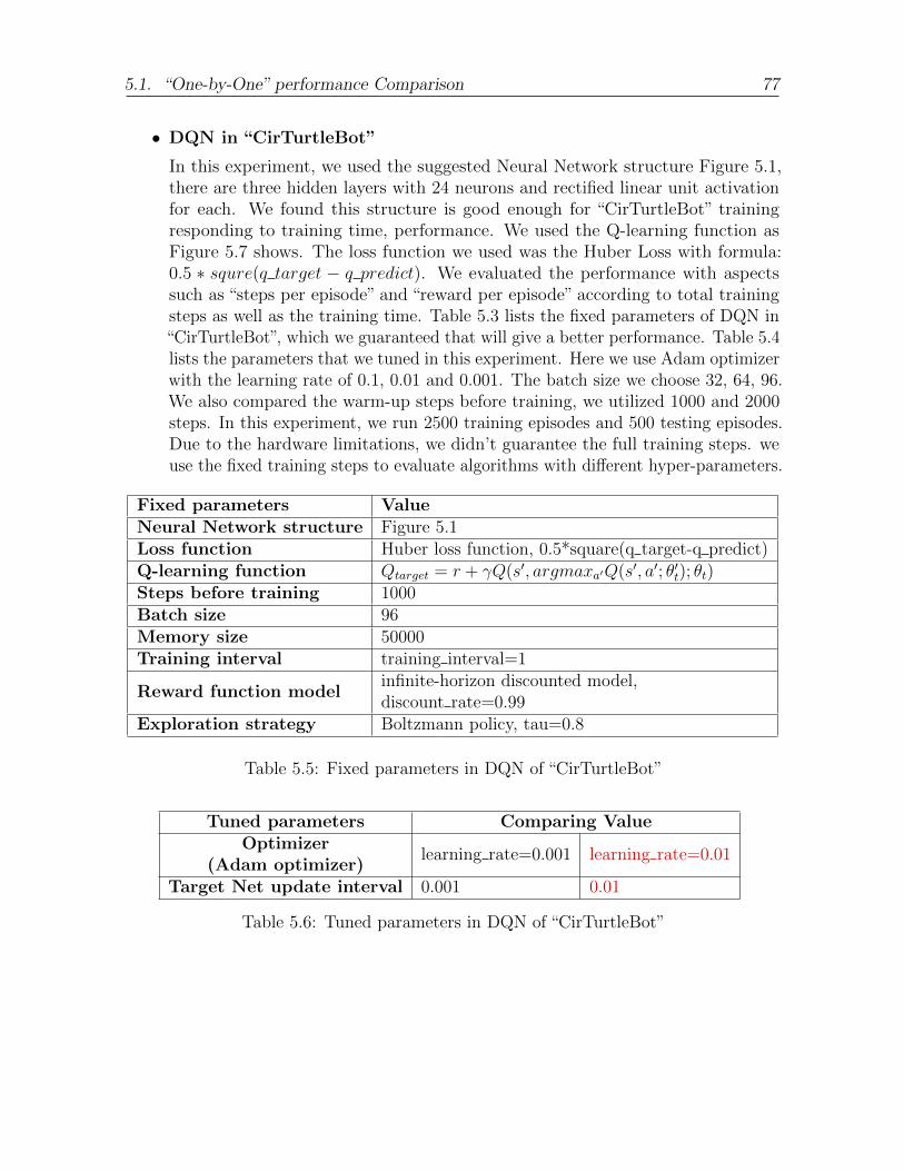
5.1. “One-by-One” performance Comparison 77
• DQN in “CirTurtleBot”
In this experiment, we used the suggested Neural Network structure Figure 5.1,there are three hidden layers with 24 neurons and rectified linear unit activationfor each. We found this structure is good enough for “CirTurtleBot” trainingresponding to training time, performance. We used the Q-learning function asFigure 5.7 shows. The loss function we used was the Huber Loss with formula:0.5 ∗ squre(q target − q predict). We evaluated the performance with aspectssuch as “steps per episode” and “reward per episode” according to total trainingsteps as well as the training time. Table 5.3 lists the fixed parameters of DQN in“CirTurtleBot”, which we guaranteed that will give a better performance. Table 5.4lists the parameters that we tuned in this experiment. Here we use Adam optimizerwith the learning rate of 0.1, 0.01 and 0.001. The batch size we choose 32, 64, 96.We also compared the warm-up steps before training, we utilized 1000 and 2000steps. In this experiment, we run 2500 training episodes and 500 testing episodes.Due to the hardware limitations, we didn’t guarantee the full training steps. weuse the fixed training steps to evaluate algorithms with different hyper-parameters.
Fixed parameters ValueNeural Network structure Figure 5.1Loss function Huber loss function, 0.5*square(q target-q predict)Q-learning function Qtarget = r + γQ(s′, argmaxa′Q(s′, a′; θ′t); θt)Steps before training 1000Batch size 96Memory size 50000Training interval training interval=1
Reward function modelinfinite-horizon discounted model,discount rate=0.99
Exploration strategy Boltzmann policy, tau=0.8
Table 5.5: Fixed parameters in DQN of “CirTurtleBot”
Tuned parameters Comparing ValueOptimizer
(Adam optimizer)learning rate=0.001 learning rate=0.01
Target Net update interval 0.001 0.01
Table 5.6: Tuned parameters in DQN of “CirTurtleBot”

78 5. Evaluation and results
As Table 5.6 shows, we evaluated the ’learning rate’ and ’target net updateinterval’ factors. Figure 5.10 shows the performance of two different learn-ing rate: 0.001, 0.01 with fixed target net update=0.01. Figure 5.11 showsthe performance of two different target net update interval: 0.001, 0.01 withfixed learning rate=0.01. Because the vibration amplitude of the three curvesis really large, we separate the comparison to two figures. The red line rep-resents learning rate=0.01, target net update=0.01; the blue line representslearning rate=0.001, target net update=0.01; the green line represents learn-ing rate=0.01, target net update=0.001.
In Figure 5.10, two lines coverage both at around 15000 steps. The red lineoscillates between 400 and 850 rewards, the blue line oscillates between 0 and 1200rewards. Although the blue line performs a higher score than the red one, it isnot stabler than the red one. In real engineering applications, we rather like theperformance of the red one. In Figure 5.11, the red line coverages faster and itis stabler than the green on. Since we can’t get higher performance using thismethod, we would admit that the red one which represents learning rate=0.01,target net update=0.01 has the highest performance. This is similar to the casefor PlaneBall.
Figure 5.9: DQN-CirturtleBot: Training time

5.1. “One-by-One” performance Comparison 79
Fig
ure
5.10
:D
QN
-Cir
turt
leB
ot:
Explo
rati
onst
rate
gyan
ddis
counte
dra
teco
mpar
ison

80 5. Evaluation and results
Figu
re5.11:
DQ
N-C
irturtleB
ot:E
xploration
strategyan
ddiscou
nted
ratecom
parison

5.1. “One-by-One” performance Comparison 81
5.1.2 DDPG method in the environments
In our evaluation, we evaluate the DDPG method for three environments, we tunedthe hyperparameters to compare the performance. The hyper-parameters in the DDPGalgorithm are presented in Figure 5.14. We used the actor-critic neural network archi-tectures as Figure 5.12, Figure 5.13 show. The input and output layers are, naturally,different for different environments with different observation spaces.
Figure 5.12: Actor Neural Network architecture of DDPG

82 5. Evaluation and results
Figure 5.13: Critic Neural Network architecture of DDPG

5.1. “One-by-One” performance Comparison 83
Fig
ure
5.14
:H
yp
er-p
aram
eter
sin
DD
PG

84 5. Evaluation and results
• DDPG in “CartPole”
We trained the DDPG agent in “CartPole” in 300000 training steps. When theagent triggers the termination condition it will stop training and be performingthe test during the remaining steps. In “CartPole”, the termination condition isdefined as holding 200 rewards in 10 episodes. Table 5.7 and Table 5.8 describethe fixed parameters and tuned parameters respectively. We used the actor-criticneural network architectures in Figure 5.12 and Figure 5.13, with four-dimensionalobservation space and one dimensional action space.
Fixed parameters ValueNeural Network structure Figure 5.12, Figure 5.13Critic learning rate 0.001Steps before training 1000Batch size 96Target Net update interval 0.001Training interval training interval=1
Reward function modelinfinite-horizon discounted model,discount rate=0.99
Exploration strategy(Random process)
OrnsteinUhlenbeckProcess
Table 5.7: Fixed parameters in DDPG of “CartPole”
Tuned parameters Comparing ValueActor learning rate learning rate=0.001 learning rate=0.00001
memory size memory=50000 memory=10000
Table 5.8: Tuned parameters in DDPG of “CartPole”
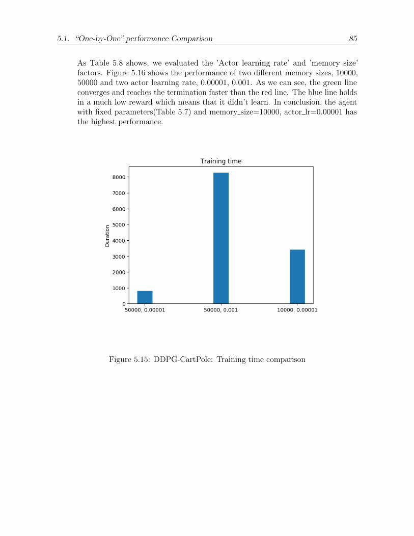
5.1. “One-by-One” performance Comparison 85
As Table 5.8 shows, we evaluated the ’Actor learning rate’ and ’memory size’factors. Figure 5.16 shows the performance of two different memory sizes, 10000,50000 and two actor learning rate, 0.00001, 0.001. As we can see, the green lineconverges and reaches the termination faster than the red line. The blue line holdsin a much low reward which means that it didn’t learn. In conclusion, the agentwith fixed parameters(Table 5.7) and memory size=10000, actor lr=0.00001 hasthe highest performance.
Figure 5.15: DDPG-CartPole: Training time comparison

86 5. Evaluation and results
Figu
re5.16:
DD
PG
-CartP
ole:m
emory
sizean
dactor
learnin
grate
comparison

5.1. “One-by-One” performance Comparison 87
• DDPG in “PlaneBall”
We trained the DDPG agent in “PlaneBall” in 500000 training steps. When theagent triggers the termination condition, it will stop training and be performingthe test during the remaining steps. In “PlaneBall”, the termination condition isdefined as holding 800 rewards in 10 episodes. Table 5.9 and Table 5.10 describethe fixed parameters and tuned parameters respectively. We used the actor-criticneural network architectures in Figure 5.12 and Figure 5.13 with seven dimensionalobservation space and two dimensional action space.
Fixed parameters ValueNeural Network structure Figure 5.12 Figure 5.13Critic learning rate 0.001Memory size 50000Steps before training 1000Batch size 96Training interval training interval=1
Reward function modelinfinite-horizon discounted model,discount rate=0.99
Exploration strategy(Random process)
OrnsteinUhlenbeckProcess
Table 5.9: Fixed parameters in DDPG of “PlaneBall”
Tuned parameters Comparing ValueActor learning rate actor lr=0.00001 actor lr=0.001
Target net update interval target update=0.001 target update=0.01
Table 5.10: Tuned parameters in DDPG of “PlaneBall”

88 5. Evaluation and results
As Table 5.10 shows, we evaluated the ’Actor learning rate’ and ’target net updateinterval’ factors. Figure 5.18 shows the performance of two different actor learningrate, 0.00001, 0.001 and two target net update interval, 0.001, 0.01. As we cansee, green line converges and reach the termination faster, but the reward in thetest phase is smaller than the red line. This means that the green line was not fullytrained. The blue line holds in a much low reward which means that it didn’t learn.In conclusion, the agent with fixed parameters(Table 5.9) and actor lr=0.00001,target net update=0.001 has the best performance.
Figure 5.17: DDPG-PlaneBall: Training time comparison

5.1. “One-by-One” performance Comparison 89
Fig
ure
5.18
:D
DP
G-P
laneB
all:
acto
rle
arnin
gra
tean
dta
rget
net
up
dat
ein
terv
alco
mpar
ison

90 5. Evaluation and results
• DDPG in “CirTurtleBot”
We trained the DDPG agent in “CirTurtleBot” in 200000 training steps. When theagent triggers the termination condition it will stop training and be performingthe test during the rest steps. In “PlaneBall”, the termination condition is definedas holding 600 rewards in 10 episodes. Table 5.11 and Table 5.12 describe thefixed parameters and tuned parameters respectively. We used the actor-criticneural network architectures in Figure 5.12 and Figure 5.13 with 20 dimensionalobservation space and one dimensional action space.
Fixed parameters ValueNeural Network structure Figure 5.12 Figure 5.13Target net update interval 0.001Memory size 50000Steps before training 1000Batch size 96Training interval training interval=1
Reward function modelinfinite-horizon discounted model,discount rate=0.99
Exploration strategy(Random process)
OrnsteinUhlenbeckProcess
Table 5.11: Fixed parameters in DDPG of “CirTurtleBot”
Tuned parameters Comparing ValueActor learning rate actor lr=0.0001 actor lr=0.00001Critic learning rate critic lr=0.001 critic lr=0.01
Table 5.12: Tuned parameters in DDPG of “CirTurtleBot”

5.1. “One-by-One” performance Comparison 91
As Table 5.12 shows, we evaluated the ’Actor learning rate’ and ’Critic learningrate’ factors. Figure 5.18 shows the performance of two different actor learningrate, 0.00001, 0.0001 and two critic learning rate, 0.001, 0.01. The red line repre-sents actor lr=0.0001, critic lr=0.001; the blue line represents actor lr=0.00001,critic lr=0.001; the green line represents actor lr=0.00001, critic lr=0.01.
As we can see, the red line coverages faster than the other two, it reaches stableat around 26000 steps. After reaching the termination, the red line holds around1000 scores, the blue line and the green hold around 900 and 800 scores separately.Therefore, the red line shows the better performance. In conclusion, the agent withfixed parameters(Table 5.11) and actor lr=0.0001, critic lr=0.001 has a higherperformance.
Figure 5.19: DDPG-CirTurtleBot: Training time comparison

92 5. Evaluation and results
Figu
re5.20:
DD
PG
-CirT
urtleB
ot:actor
learnin
grate
and
targetnet
up
date
interval
comparison

5.1. “One-by-One” performance Comparison 93
5.1.3 PPO method in the environments
In this evaluation we evaluate the Distributed PPO method for three environments, wetuned the hyperparameters to compare the performance. The hyper-parameters in theDPPO algorithm are presented in Figure 5.21. For this method, we combined bothPPO and A3C, where we optimize the “clipped surrogate objective” using a numberof samples collected by several parallel workers. There is a global PPO brain used forupdating, each worker (agent) run in its own environment at the same time and uploadthe collected samples to the global brain. The workers should wait until the global brainfinish updating after every batch size samples. We used the actor-critic neural networkarchitectures as Figure 5.12, Figure 5.13 show. The input and output layers are differentregarding different environments.

94 5. Evaluation and results
Figu
re5.21:
Hyp
er-param
etersin
DP
PO

5.1. “One-by-One” performance Comparison 95
• PPO in “CartPole”
We trained the DDPG agent in “CartPole” in 300000 training steps.Table 5.13 andTable 5.14 describe the fixed parameters and tuned parameters respectively. Weused the actor-critic neural network architectures in Figure 5.12 and Figure 5.13,with four dimensional observation space and a one dimensional action space.
Fixed parameters ValueNeural Network structure Figure 5.12, Figure 5.13Constrain methods Clipped surrogate objectiveActor learning rate 0.0001Critic learning rate 0.00002Loop update steps (10,10)number of workers 4
Reward function modelinfinite-horizon discounted model,discount rate=0.99
Exploration random samples from a normal distribution
Table 5.13: Fixed parameters in DPPO of “CartPole”
Tuned parameters Comparing ValueClipped surrogate epsilon epsilon=0.2 epsilon=0.8
Batch size batch size = 32 batch size=320
Table 5.14: Tuned parameters in DPPO of “CartPole”
As Table 5.14 shows, we evaluated the ’Clipped surrogate epsilon’ and ’batchsize’ factors. Figure 5.23 shows the performance of two different batch sizes, 32,320 and two clipped surrogate epsilon, 0.2, 0.8. Here, the batch size factor hasanother meaning comparing to other methods. It means that after every batch sizeexamples which are collected by all the parallel workers, the PPO brain will updateonce. The ’Clipped surrogate epsilon’ factor is a hyper-parameter in PPO, whichwe described in Chapter 2.
As we can see, the blue line and the green line appeared in fault curves. Afteraround 30000 steps, the two lines increase rapidly and staying in 150 rewardsfor a short time, then increase and hold to 200 rewards. Relatively, the greenline raised faster and held the highest score earlier than the blue one. Thered line also coverages fast, but the score is not stable all the time. The redline represents algorithm with batch size = 320, epsilon = 0.2, the green linerepresents algorithm with batch size = 32, epsilon = 0.2, the blue line representsalgorithm with batch size = 32, epsilon = 0.8. In conclusion, the agent with fixedparameters(Table 5.13) and batch size=32, epsilon=0.8 has a high performance.

96 5. Evaluation and results
Figure 5.22: DPPO-CartPole: Training time comparison

5.1. “One-by-One” performance Comparison 97
Fig
ure
5.23
:D
PP
O-C
artP
ole:
bat
chsi
zean
dcl
ipp
edsu
rrog
ate
epsi
lon
com
par
ison

98 5. Evaluation and results
• PPO in “PlaneBall”
We trained the PPO agent in “PlaneBall” in 500000 training steps. Table 5.15 andTable 5.16 describe the fixed parameters and tuned parameters respectively. Weused the actor-critic neural network architectures in Figure 5.12 and Figure 5.13,with seven dimensional observation space and two dimensional action space.
Fixed parameters ValueNeural Network structure Figure 5.12, Figure 5.13Constrain methods Clipped surrogate objective, epsilon=0.2Actor learning rate 0.00001Critic learning rate 0.0001number of workers 4
Reward function modelinfinite-horizon discounted model,discount rate=0.99
Exploration random samples from a normal distribution
Table 5.15: Fixed parameters in DPPO of “PlaneBall”
Tuned parameters Comparing Value
Loop update stepsactor update steps=10critic update steps=100
actor update steps=100critic update steps=100
Batch size batch size = 200 batch size=100
Table 5.16: Tuned parameters in DPPO of “PlaneBall”
As Table 5.16 shows, we evaluated the ’Loop update steps’ and ’batch size’ factors.Figure 5.25 shows the performance of two different batch size, 100, 200 and twoloop update steps, (10,100), (100,100). The ’Loop update steps’ factor is a hyper-parameter in PPO, which means that, the looping steps when global PPO doingthe update. We defined actor update steps and critic update steps separately. Wecompare the combination of actor update steps=10, critic update steps=100, andactor update steps=100, critic update steps=100. Here, the batch size factor hasanother meaning comparing to other methods. It means that after every batch sizeexamples which collected by all the parallel workers, the PPO brain will updateonce.
As we can see, both the blue line and the red line appeared to learn after around150000 steps. The blue line holds the stable average score after 200000 steps witharound 650 average score. The red line holds the stable average score after 400000steps with around 500 average score. Comparing the two, the blue line shows thebetter performance than the red one regarding the convergence speed and theaverage score. The green line didn’t learn because it oscillates between -250 to250 during the training steps.
The red line represents the algorithm with batch size = 100, update steps=(10,100),the green line represents algorithm with batch size = 200, update steps=(100,100),

5.1. “One-by-One” performance Comparison 99
the blue line represents the algorithm with batch size = 200, and update steps=(10,100).In conclusion, the agent with fixed parameters(Table 5.15) and batch size = 200,update steps=(10,100) has a the highest performance.
Figure 5.24: DPPO-PlaneBall: Training time comparison

100 5. Evaluation and results
Figu
re5.25:
DP
PO
-Plan
eBall:
batch
sizean
dlo
opup
date
steps
comparison

5.1. “One-by-One” performance Comparison 101
• PPO in “CirTurtleBot”
We trained the DDPG agent in “CirTurtleBot” in 200000 training steps. Table 5.17and Table 5.18 describe the fixed parameters and tuned parameters respectively.We used the actor-critic neural network architectures in Figure 5.12 and Figure 5.13,with 20 dimensional observation space and one dimensional action space.
Fixed parameters ValueNeural Network structure Figure 5.12, Figure 5.13Constrain methods Clipped surrogate objectiveActor learning rate 0.0001Critic learning rate 0.00002Batch size 32number of workers 2Clipped surrogate epsilon 0.2
Reward function modelinfinite-horizon discounted model,discount rate=0.99
Exploration random samples from a normal distribution
Table 5.17: Fixed parameters in DPPO of “CirTurtleBot”
Tuned parameters Comparing Value
Loop update stepsactor update steps=10critic update steps=10
actor update steps=1critic update steps=10
actor update steps=1critic update steps=10
Table 5.18: Tuned parameters in DPPO of “CirTurtleBot”
As Table 5.18 shows, we evaluated the ’Loop update steps’ factor with three combi-nations: (actor update steps=10, critic update steps=10), (actor update steps=1,critic update steps=10), (actor update steps=10, critic update steps=1). Fig-ure 5.27 shows the performance of these three different loop update steps combi-nations’ comparison.
As we can see, the blue line oscillates around 100, it didn’t learn during the 200ksteps. The red line converges to its high score in around 150000 steps with 1300rewards. The green line coverages to its high score in around 75000 steps with1300 rewards. Although the red line and the green line have the same high scorein general, the green line converges faster than the red one. In contrast, aftercoverage, the red line is more stable than the green one.
The red line represents algorithm with (actor update steps=10, critic update steps=10),the green line represents the algorithm with (actor update steps=10, critic update steps=1),the blue line represents the algorithm with (actor update steps=1, critic update steps=10).In conclusion, the agent with fixed parameters(Table 5.17) and (actor update steps=10,critic update steps=1) has the best performance.

102 5. Evaluation and results
Figure 5.26: DPPO-CirTurtleBot: Training time comparison
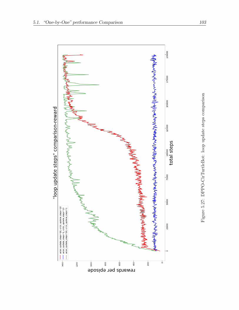
5.1. “One-by-One” performance Comparison 103
Fig
ure
5.27
:D
PP
O-C
irT
urt
leB
ot:
loop
up
dat
est
eps
com
par
ison

104 5. Evaluation and results
5.2 Methods comparison through environments
In this evaluation section, we focus on the second research question. We compare thethree methods with a high performance guarantee (based on the studies in the previoussection). We list all the meta-parameters which we tuned for high performance inTable 5.19.
We evaluated the three methods regarding:
• Time complexityWith fixed training steps, we compare the running time among the three methods.
• Sample efficiencySample efficiency is an important criterion in training performance comparison.During the training phases, the method which coverages faster has the highersample efficiency.
• Highest and average scoreThe highest and average score of the training are intuitive ways for performanceevaluation.
• robustnessRobustness here means the offset amplitude around the highest score, for the fullytrained agent.

5.2. Methods comparison through environments 105
Enti
tyP
ara
mete
rV
alu
ein
Cart
Pole
Valu
ein
Pla
neB
all
Valu
ein
Cir
Tu
rtle
Bot
DQ
N
lear
nin
gra
tem
emor
ysi
zew
arm
up
step
sbat
chsi
zeta
rget
net
up
dat
etr
ain
inte
rval
dis
count
rate
explo
rati
on
0.00
110
000
2000
64 0.01
1 0.99
Bol
tzm
ann
(tau
=1)
0.01
1000
0020
000
640
0.01
1 0.99
Bol
tzm
ann
(tau
=1)
0.00
110
000
2000
64 0.01
1 0.99
Bol
tzm
ann
(tau
=1)
DD
PG
acto
rlr
crit
iclr
mem
ory
size
war
mup
step
sbat
chsi
zeta
rget
net
up
dat
etr
ain
inte
rval
dis
count
rate
explo
rati
on
0.00
001
0.00
110
000
1000
96 0.00
11 0.
99O
rnst
einU
hle
nb
eck
(thet
a=0.
15,
mu=
0,si
gma=
0.3)
0.00
001
0.00
150
000
1000
96 0.00
11 0.
99O
rnst
einU
hle
nb
eck
(thet
a=0.
15,
mu=
0,si
gma=
0.3)
0.00
010.
001
5000
010
0032 0.
001
1 0.99
Orn
stei
nU
hle
nb
eck
(thet
a=0.
15,
mu=
0,si
gma=
0.3)
DP
PO
acto
rlr
crit
iclr
bat
chsi
zedis
count
rate
loop
up
dat
est
eps
explo
rati
onco
nst
rain
met
hod
num
wor
kers
0.00
010.
0000
232 0.
99(1
0,10
)ra
ndom
sam
ple
sfr
oma
nor
mal
dis
trib
uti
oncl
ipp
edsu
rrog
ate
obje
ctiv
e,ep
silo
n=
0.2
4
0.00
001
0.00
0120
00.
99(1
0,10
0)ra
ndom
sam
ple
sfr
oma
nor
mal
dis
trib
uti
oncl
ipp
edsu
rrog
ate
obje
ctiv
e,ep
silo
n=
0.2
4
0.00
001
0.00
0132 0.
99(1
0,1)
random
sam
ple
sfr
oma
nor
mal
dis
trib
uti
oncl
ipp
edsu
rrog
ate
obje
ctiv
e,ep
silo
n=
0.2
2
Tab
le5.
19:
Met
a-par
amet
erof
DQ
N,
DD
PG
,D
PP
Oov
erth
ree
envir
onm
ents

106 5. Evaluation and results
5.2.1 Comparison in “CartPole”
We evaluate the performance of DQN, DDPG and DPPO in the CartPole environment.The hyper-parameters of these three methods are chosen from the first evaluation sectionwith relatively high performance guarantees. We trained in 300k steps, and generatethe curves of ’episode reward’ responding to ’total steps’, as Figure 5.29 shows. Inthis figure, the red line represents DQN, the blue line represents DDPG, the green linerepresents DPPO. Among these three methods, DQN converges faster than the othertwo, it reached the highest score(200) at around 25000 steps. DPPO and DDPG reachedthe highest score in around 40000 and 170000 steps. This means DQN has better sampleefficiency than the other two. After reaching the highest score, DQN didn’t hold 200 forthe whole steps, it appeared to get 197 scores in few steps. Instead, DPPO and DDPGboth hold the highest score after the first time reaching it, therefore the methods scorehigher in robustness. Figure 5.28 shows the training time among these three methods.DPPO had the least training time, DDPG had the most training time with more than4000 seconds. Both DQN and DPPO had a quite less training time with 800 and 500seconds. In conclusion, DDPG showed the worst performance than DQN and DDPGresponding to time complexity, sample complexity. DQN had better sample complexitythan DPPO but had worse robustness.
Figure 5.28: CartPole: Training time comparison

5.2. Methods comparison through environments 107
Fig
ure
5.29
:C
artP
ole:
DQ
N,
DD
PG
,D
PP
Oco
mpar
ison

108 5. Evaluation and results
5.2.2 Comparison in “PlaneBall”
We evaluate the performance of DQN, DDPG and DPPO in the PlaneBall environment.The hyper-parameters of these three methods are chosen from the first evaluation sectionwith relatively high performance guarantees. We trained in 500k steps, and generate thecurves of ’episode reward’ responding to ’total steps’, as Figure 5.31 shows. In this figure,the red line represents DQN, the blue line represents DDPG, the green line representsDPPO. Among these three methods, DDPG converges faster than the other two, itreached the highest score(900) at around 180000 steps. DPPO and DQN reached thehighest score in around 200000 and 300000 steps. This means DDPG has better sampleefficiency than the other two. Obviously, DDPG holds the higher score with around 700,than the other two during the training steps. DPPO vibrates around 500 scores afterconvergence. DQN didn’t really learn in 50k steps. According to the hyper-parametertunning of DQN in PlaneBall in the first evaluation section, the DQN agent learnedafter 1000k steps.
Figure 5.30 shows the training time among these three methods. DPPO had the leasttraining time, DQN had the most training time of more than 40000 seconds. BothDDPG and DPPO had a quite less training time with 8000 and 1000 seconds. Inconclusion, DDPG showed the best performance than DQN and DPPO responding totime complexity, sample complexity and high score.
Figure 5.30: PlaneBall: Training time comparison

5.2. Methods comparison through environments 109
Fig
ure
5.31
:P
laneB
all:
DQ
N,
DD
PG
,D
PP
Oco
mpar
ison

110 5. Evaluation and results
5.2.3 Comparison in “CirTurtleBot”
We evaluate the performance of DQN, DDPG and DPPO in CirTurtleBot environment.The hyper-parameters of these three methods are chosen from the first evaluation sectionwith relatively high performance guarantees. We trained in 200k steps, and generatethe curves of ’episode reward’ responding to ’total steps’, as Figure 5.33 shows. Inthis figure, the red line represents DQN, the blue line represents DDPG, the greenline represents DPPO. Among these three methods, DDPG converges faster than theother two, it reached its highest score(1100) at around 30000 steps. DPPO reached itshighest score(1300) in around 75000 steps. DQN oscillate between 250 and 1000 after20000 steps. This means that DQN didn’t learn well in 200k steps. Besides, DDPG hasbetter sample efficiency than DPPO but the high score and average score are lower thanDPPO.
Figure 5.32 shows the training time among these three methods. DPPO had the leasttraining time, DQN had the most training time with more than 8000 seconds. BothDDPG and DPPO had a quite less training time with 5000 and 3000 seconds. Inconclusion, DPPO showed the best performance than DQN and DDPG responding totime complexity, higher score an average score. DDPG had better sample efficiency androbustness than DPPO.
Figure 5.32: CirTurtleBot: Training time comparison

5.2. Methods comparison through environments 111
Fig
ure
5.33
:C
irT
urt
leB
ot:
DQ
N,
DD
PG
,D
PP
Oco
mpar
ison

112 5. Evaluation and results
5.3 Summary
In this chapter, evaluation and results are discussed regarding the research questions.
For the first research question we found that hyper-parameters have a high impact, andthus need to be reported in oder to understand the results of a benchmark. We werespecifically able to ascertain experimentally the important effect of exploration policiesand their parameters, update rate to target networks, memory sizes, actor critic learningrate and batch size in PPO.
With high performance guaranteed algorithms, for ’CartPole’, DQN and DPPO bothhave higher performance; for ’PlaneBall’, DDPG has the highest performance, DQNcouldn’t learn in 500k steps, and its training is much higher than the other two; for’CirTurtleBot’, DDPG and DPPO both have higher performance, DPPO has a higherscore and lower training time. DDPG is robust and has better sample efficiency. However,there are many threats in our experiments which have influences on the results validity,we will discuss these in Chapter 7 in detail.
In the next chapter, related work will be discussed and compared.

6. Related work
In this chapter, we review papers and work that is similar to our task, and existingresearch in benchmarks for deep reinforcement learning. We first discuss literature ofRL in applications, then come to challenges, last but not least, the released benchmarks.
6.0.1 Engineering Applications
Some papers have researched Deep Reinforcement Learning in applications. [LWR+17]first presents the general DRL framework, then introduces three specific engineeringapplications: the cloud computing resource allocation problem, the residential smartgrid task scheduling problem, and building HVAC system optimal control problem.The effectiveness of the DRL technique in these three cyber-physical applicationshave been validated. Finally, the paper studies on the stochastic computing-basedhardware implementations of the DRL framework, which constitutes an improvementin area efficiency and power consumption compared with binary-based implementationcounterparts. Comparing this research with our work, we also list three applicationsthat intend to represent engineering tasks of varying complexity, however, we focus onspecific DRL methods, and we provide a comparative evaluation.
In recent work [PR96], a new algorithm called C-Trace, a variant of the P-Trace RLalgorithm is introduced, and some possible advantages of using algorithms of this type arediscussed. Authors also present experimental results from three domains: A simulatednoisy pole-and-cart system, an artificial non-Markovian decision problem, and a realsix-legged walking robot. The results from each of these domains suggest that thatactual return (Monte Carlo) approaches to the credit-assignment problem may be moresuited than temporal difference (TD) methods for many real-world control applications.Comparing to our work, we also use a cart-pole system as the experimental environment,engineering control applications are also our main focus. However, the algorithms weimplement are recent Deep RL algorithms, and we focus solely on the comparison ofthese methods with regards to their sensitivity to hyper-parameter configuration issues.

114 6. Related work
Similar to our work, in [Cap18], recent Deep RL methods like Deep Q Network, DeepDeterministic Policy Gradient and Asynchronous Advanced Actor Critic are presented indetail. Starting with traditional reinforcement learning concepts, methods, authors cometo deep reinforcement learning and function approximation. Two industrial applications,robotics and autonomous driving, are utilized for experiments. The testbeds are aDouble Inverted Pendulum , Hopper and a TORCS simulator. The DDPG and A3Cmethods are implemented and evaluated in these three environments. Comparing withour work, we too present state-of-the-art Deep RL methods DDPG and A3C, and oneexperimental environment. We also present DQN and PPO, and evaluate these methodson three environments: “CartPole”, “PlaneBall”, “CirTurtleBot”. Our environments arechosen such that they can encompass different aspects of engineering application. Thegoal of our task is to provide results on the practical criteria that needs to be considered(hyper-parameter disclosure, and essential metrics per method) for further Deep RL inengineering application benchmark design.
6.0.2 Challenges of RL in Engineering Applications
There is preceding work to ours which is concerned only in the field of robotics [PN17,KCC13, PVS03, Mat97, KBP13b], which is one of the important Deep RL applicationdomains within engineering applications. In robotics, the ultimate goal of reinforcementlearning is to endow robots with the ability to learn, improve, adapt and reproducetasks with dynamically changing constraints based on exploration and autonomouslearning. Since robotic applications are more complex and hard to apply DRL into them,the existing research focuses on implementing DRL in the robotic field and in makingcomprehensive analysis. In [KCC13], authors give a summary of the state-of-the-artof reinforcement learning in the context of robotics. Numerous challenges faced bythe policy representation in robotics are identified. Three recent examples for theapplication of reinforcement learning to real-world robots are described: a pancakeflipping task, a bipedal walking energy minimization task and an archery-based aimingtask. In all examples, a state-of-the-art expectation-maximization-based reinforcementlearning is used, and different policy representations are proposed and evaluated for eachtask. The proposed policy representations offer viable solutions to six rarely-addressedchallenges in policy representations: correlations, adaptability, multi-resolution, globality,multi-dimensionality and convergence. Both the successes and the practical difficultiesencountered in these examples are discussed. Finally, conclusions are drawn about thestate-of-the-art and the future directions for reinforcement learning in robotics.
In [KBP13b], challenges of RL in robotics are discussed with four aspects: Curse ofDimensionality, Curse of Real-World Samples, Curse of Under-Modeling and ModelUncertainty, and finally, the Curse of Goal Specification. In our paper, we discussedthe challenges of RL in applications that, when considering the real world counterparts,are also facing the aforementioned aspects. Differently, we also present other challengesregarding to general engineering applications but in more simple, simulated environment.

115
6.0.3 Benchmarks for RL
To build on recent progress in reinforcement learning, the research community needsgood benchmarks on which to compare algorithms. A variety of benchmarks have beenreleased, such as the Arcade Learning Environment(ALE)[BNVB13] which is currentlypopular benchmark, offering a collection of Atari 2600 games as reinforcement learningproblems, and recently the RLLab benchmark for continuous control[DCH+16]. Thereare also RL benchmarks regarding different comparison aspects, like[GDK+15, TW09,AV15, AV15, DEK+05, dBS16].
The Arcade Learning Environment(ALE)[BNVB13] is nowadays a well-known benchmark.The Arcade Learning Environment (ALE) is generated as a new challenge problem,platform, and experimental methodology for empirically assessing agents designed forgeneral competency. ALE is a software framework for interfacing with emulated Atari2600 game environments. It also provides a strict testbed for evaluating and comparingapproaches. ALE is released as free, open-source software, the latest version of thesource code is publicly available at: http://arcadelearningenvironment.org. Authorsprovide the benchmark results using SARSA(λ), which is a traditional RL method.Based on this method, they generated five different feature representation approaches:Basic, BASS, DISCO, LSH, RAM. The cumulative rewards are compared among theseapproaches. They first constructed two sets of games, one for training and the other fortesting. They used the training games for parameter tuning as well as design refinements,and the testing games for the final evaluation of our methods.Comparing to our work,in terms of environments, we are concerned more in simulated environments which canbe applied to engineering applications. In terms of RL methods, we used recent DeepRL methods. With regards to the comparison criteria, cumulative reward was not theonly criteria that we considered, but we report other factors like algorithm robustness,running time, etc.
In 2016, another RL benchmark for continuous control[DCH+16] was released. Since mostwork in ARCADE [BNVB13] was targeting aim algorithms designed for tasks with high-dimensional state inputs and discrete actions, there was a gap regarding the comparisonof algorithms for environments with continuous action spaces. This novel benchmarkconsists of 31 continuous control tasks with Basic Tasks, locomotion tasks, PartiallyObservable Tasks and Hierarchical Tasks. Nine RL algorithms were implemented inthe benchmark, they are: Random, REINFORCE, TNPG, RWR, REPS, TRPO, CEM,CMEA-ES, DDPG. They also provide more criteria for the comparison when comparedto ARCADE, such like the iteration numbers of each algorithm, average reward, etc.All the source code and the agents are made publicly available rllab1. Comparingto our work, our aim is to provide practical criteria to make comparisons regardingengineering application features. Alongside, the algorithms we used for experimentsare DQN, DDPG, and DPPO, which are recently released Deep RL algorithm. In theaspect of environments, we also choose them from simple classical control problems, likethe CartPole system to a Hierarchical robotic Task.
1http://ray.readthedocs.io/en/latest/index.html

116 6. Related work
There is also related wok [dBS16] dedicated to comparing the sample complexity of RLalgorithms. Authors have proposed that in robotics, improving some cost function inorder to reach the controller efficiency generally requires to perform many evaluations ofcontrollers on the real robot with different parameter values. This process is often timeconsuming, it may lead to abrasion of the mechanical structure or even to damage if thetested controllers generate dangerous behaviors. As a result, sample efficiency is a crucialproperty of any robot learning method. This paper implemented Deep DeterministicPolicy Gradient(DDPG) and Covariance Matrix Adaptation Evolution Strategy (CMA-ES) algorithms, and are evaluated on a continuous version of the mountain car problem.Based on their evaluations, the general finding is that DDPG requires far less interactionswith the environment than CMA-ES and with less variance between different runs. Thereason of choosing DDPG and CMA-ES is that, DDPG is a Deep RL method based onactor-critic policy estimation approach, CMA-ES is a direct policy search method. Theirevaluation could be understood as the comparison between two very different kinds ofRL methods. Comparing with our work, we also did the evaluation with respect tosample complexity. Rather than that, we also compared other factors like robustness,time complexity, and the implemented algorithms are DQN, DDPG, and DPPO whichare currently competitive methods.
6.1 Summary
In this chapter, we present a comparative review on work that is similar to our research.
In next chapter, we give conclusions about our work and the drawbacks which need tobe improved.

7. Conclusions and future work
In this chapter, we summarize all our work and give some general ideas for further work.
7.1 Work summary
In this work, the most popular deep reinforcement learning methods are comparedin three representative engineering tasks (CartPole, PlaneBall, CirTurtleBot). Thealgorithms include DQN, DDPG and DPPO with deep neural networks as policyrepresentation. In order to break the gap of comparison between discrete task methodand continuous task method, we implemented both discrete and continuous version foreach environment.
In the evaluation, we perform two kinds of comparisons regarding two research questions.First of all we did a hyper-parameter comparison, where methods were compared one byone. We evaluate one method in one environment, comparing the method with differenthyper-parameters’ values, choosing by the end the values that result in the highestperformance. After that, we compared different methods with high performance hyper-parameters in one specific environment. During the second comparison, we evaluatethese methods with regards to training time, sample efficiency and robustness.
According to our evaluation, the DQN method had the higher performance only in the“CartPole” environment. This environment is famous as a classical problem with lowdimension space. We can assume that, in engineering problems, if we can generatethose problems as a low dimension training model, DQN is a good choice for training.DDPG had the higher performance in “CirTurtleBot” environment, and especially in“PlaneBall” environment which has the highest dimension and did the worst in “CartPole”environment. We may consider using DDPG for a higher dimension engineering modeltraining. DPPO showed the relative higher performance among these three environments.It seems like it is suitable for both low and high dimension models. However, if we useDPPO in engineering problems, we should also take the hardware and training cost into

118 7. Conclusions and future work
consideration, Because the performance of DPPO relies on the workers’ number andthus requires more computational power. This means that it needs better hardwaresupport than the other two methods. The training time and robustness of DPPO aredependent on how many workers are training at the same time. In reality, if we don’thave such high hardware support for training, we could use DDPG instead.
7.2 Threats to validity
• Limitations in HardwareWe have to admit that the computer’s performance really can affect the runningtime, the training time is different for the same algorithm running on differentcomputers. And GPUs are considered to be much faster than CPUs. This mayaffect the performance of the DPPO method because we can’t train the agent withmore than 8 workers in parallel. Definitely, the training speed and accuracy willbe improved if more workers train at the same time.
• Algorithm implementationAlthough the pseudo code of the methods are proposed and we could find compa-rable implementations from different researchers, the way of code implementationhas the influence on training time. More than that, the mechanisms for optimizingthe methods are being proposed and updated with high speed, the performancecould be affected by using the newest optimization mechanism. For example,the DQN method has many variations, such as Double-DQN, Distributed DQN,Prioritized Experience Replay, and others. Recently, the DDPG method has beenupdated by a mechanism call batch normalization. PPO has two methods toconstrain the surrogate objective function. Due to the time and ability limitations,we can’t implement all the methods with the newest mechanisms. In our work, weimplemented Double-DQN, DDPG without batch normalization, DPPO with theclipped surrogate objective. This may affect the comparison performance.
• Environment designsAs we said before, we implemented both discrete and continuous versions foreach environment. The discretized size is an important issue we need to considerbecause this can affect the performance.
• Experiment setupsFirst of all, we perform 5 times for each algorithm and average them to get theresults. The result will be more accurate if taking more trials for the experiment,smoothing out variances due to the randomness in exploration and highlightingtrends with more clarity. Second, we perform 30k, 50k, 20k steps for CartPole,PlaneBall, CirTurtleBot training. It will affect the robust performance comparison.Last but not least, choosing a high performance hyper-parameters combination iscomplicated because we usually can’t compare all the possibilities of the hyper-parameters combinations due to time and computational limits.

7.3. Future work 119
7.3 Future work
• Training with a higher-performance computer, especially with GPUs.
• Taking more engineering tasks for the comparison, especially locomotion tasks,partially observable tasks, and hierarchical tasks.
• Implementing and evaluating A3C and DPPO with KL-Penalty, also newly pro-posed algorithms from now on.
• Proposing more other criteria for methods comparison.
• Benchmarking general engineering tasks.

Bibliography
[ADBB17a] Kai Arulkumaran, Marc Peter Deisenroth, Miles Brundage, and Anil An-thony Bharath. A brief survey of deep reinforcement learning. arXivpreprint arXiv:1708.05866, 2017. (cited on Page 3)
[ADBB17b] Kai Arulkumaran, Marc Peter Deisenroth, Miles Brundage, and Anil An-thony Bharath. A brief survey of deep reinforcement learning. arXivpreprint arXiv:1708.05866, 2017. (cited on Page 4)
[ADBB17c] Kai Arulkumaran, Marc Peter Deisenroth, Miles Brundage, and Anil An-thony Bharath. A brief survey of deep reinforcement learning. arXivpreprint arXiv:1708.05866, 2017. (cited on Page 23)
[AO00] M Emin Aydin and Ercan Oztemel. Dynamic job-shop scheduling usingreinforcement learning agents. Robotics and Autonomous Systems, 33(2-3):169–178, 2000. (cited on Page 53)
[AV15] Saminda Abeyruwan and Ubbo Visser. Rllib: C++ library to predict,control, and represent learnable knowledge using on/off policy reinforce-ment learning. In Robot Soccer World Cup, pages 356–364. Springer, 2015.(cited on Page 115)
[BB01] Jonathan Baxter and Peter L Bartlett. Infinite-horizon policy-gradientestimation. Journal of Artificial Intelligence Research, 15:319–350, 2001.(cited on Page 18)
[BC95] Hee Rak Beom and Hyung Suck Cho. A sensor-based navigation for a mobilerobot using fuzzy logic and reinforcement learning. IEEE transactions onSystems, Man, and Cybernetics, 25(3):464–477, 1995. (cited on Page 53)
[BCP+16] Greg Brockman, Vicki Cheung, Ludwig Pettersson, Jonas Schneider, JohnSchulman, Jie Tang, and Wojciech Zaremba. Openai gym. arXiv preprintarXiv:1606.01540, 2016. (cited on Page ix, 55, and 56)
[Bel57] Richard Ernest Bellman. Dynamic programming. 1957. (cited on Page 3)
[BK92] Hamid R Berenji and Pratap Khedkar. Learning and tuning fuzzy logiccontrollers through reinforcements. IEEE Transactions on neural networks,3(5):724–740, 1992. (cited on Page 53)

Bibliography 121
[BNVB13] Marc G Bellemare, Yavar Naddaf, Joel Veness, and Michael Bowling. Thearcade learning environment: An evaluation platform for general agents.Journal of Artificial Intelligence Research, 47:253–279, 2013. (cited on
Page 5, 6, and 115)
[Bra93] Steven J Bradtke. Reinforcement learning applied to linear quadraticregulation. In Advances in neural information processing systems, pages295–302, 1993. (cited on Page 53)
[BSA83] Andrew G Barto, Richard S Sutton, and Charles W Anderson. Neuronlikeadaptive elements that can solve difficult learning control problems. IEEEtransactions on systems, man, and cybernetics, (5):834–846, 1983. (cited
on Page 21)
[Cap18] Antonio Cappiello. Deep reinforcement learning algorithms for industrialapplications, 2018. (cited on Page 114)
[CB96] Robert H Crites and Andrew G Barto. Improving elevator performanceusing reinforcement learning. In Advances in neural information processingsystems, pages 1017–1023, 1996. (cited on Page 46)
[cla18] Stanford CS class. Cs231n: Convolutional neural networks for visualrecognition, 2018. (cited on Page 25)
[dBS16] Arnaud de Froissard de Broissia and Olivier Sigaud. Actor-critic versusdirect policy search: a comparison based on sample complexity. arXivpreprint arXiv:1606.09152, 2016. (cited on Page 115 and 116)
[DCH+16] Yan Duan, Xi Chen, Rein Houthooft, John Schulman, and Pieter Abbeel.Benchmarking deep reinforcement learning for continuous control. InInternational Conference on Machine Learning, pages 1329–1338, 2016.(cited on Page 5, 6, 59, and 115)
[DEK+05] Alain Dutech, Timothy Edmunds, Jelle Kok, Michail Lagoudakis, MichaelLittman, Martin Riedmiller, Bryan Russell, Bruno Scherrer, Richard Sut-ton, Stephan Timmer, et al. Reinforcement learning benchmarks andbake-offs ii. Advances in Neural Information Processing Systems (NIPS),17, 2005. (cited on Page 6 and 115)
[DW92] Peter Dayan and CJCH Watkins. Q-learning. Machine learning, 8(3):279–292, 1992. (cited on Page 17)
[ET16] Mohammed E El-Telbany. The challenges of reinforcement learning inrobotics and optimal control. In International Conference on AdvancedIntelligent Systems and Informatics, pages 881–890. Springer, 2016. (cited
on Page 13 and 50)
[Fin04] Steven Finch. Ornstein-uhlenbeck process. 2004. (cited on Page 65)

122 Bibliography
[FLJ+10] Chaochao Feng, Zhonghai Lu, Axel Jantsch, Jinwen Li, and MinxuanZhang. A reconfigurable fault-tolerant deflection routing algorithm basedon reinforcement learning for network-on-chip. In Proceedings of the ThirdInternational Workshop on Network on Chip Architectures, pages 11–16.ACM, 2010. (cited on Page 53)
[GDK+15] Alborz Geramifard, Christoph Dann, Robert H Klein, William Dabney,and Jonathan P How. Rlpy: a value-function-based reinforcement learningframework for education and research. Journal of Machine LearningResearch, 16:1573–1578, 2015. (cited on Page 5 and 115)
[Gly87] Peter W Glynn. Likelilood ratio gradient estimation: an overview. InProceedings of the 19th conference on Winter simulation, pages 366–375.ACM, 1987. (cited on Page 18)
[GP02] Ilaria Giannoccaro and Pierpaolo Pontrandolfo. Inventory management insupply chains: a reinforcement learning approach. International Journalof Production Economics, 78(2):153–161, 2002. (cited on Page 53)
[Ham17] Mark Hammond. Deep reinforcement learning in the enterprise: Bridgingthe gap from games to industry, 2017. (cited on Page 45, 46, 50, and 51)
[HMVH+17] Matteo Hessel, Joseph Modayil, Hado Van Hasselt, Tom Schaul, GeorgOstrovski, Will Dabney, Dan Horgan, Bilal Piot, Mohammad Azar, andDavid Silver. Rainbow: Combining improvements in deep reinforcementlearning. arXiv preprint arXiv:1710.02298, 2017. (cited on Page 4)
[Hor14] Eric Horvitz. One hundred year study on artificial intelligence: Reflectionsand framing, 2014. (cited on Page 45)
[HP04] Joonki Hong and Vittaldas V Prabhu. Distributed reinforcement learningcontrol for batch sequencing and sizing in just-in-time manufacturingsystems. Applied Intelligence, 20(1):71–87, 2004. (cited on Page 53)
[HS97] Sepp Hochreiter and Jurgen Schmidhuber. Long short-term memory. Neuralcomputation, 9(8):1735–1780, 1997. (cited on Page 28)
[HS00] Qiming He and Mark A Shayman. Using reinforcement learning for pro-active network fault management. In Communication Technology Pro-ceedings, 2000. WCC-ICCT 2000. International Conference on, volume 1,pages 515–521. IEEE, 2000. (cited on Page 53)
[HSL+17] Nicolas Heess, Srinivasan Sriram, Jay Lemmon, Josh Merel, Greg Wayne,Yuval Tassa, Tom Erez, Ziyu Wang, Ali Eslami, Martin Riedmiller, et al.Emergence of locomotion behaviours in rich environments. arXiv preprintarXiv:1707.02286, 2017. (cited on Page ix, 4, 37, and 39)
Bibliography 123
[IS15] Sergey Ioffe and Christian Szegedy. Batch normalization: Acceleratingdeep network training by reducing internal covariate shift. arXiv preprintarXiv:1502.03167, 2015. (cited on Page 35 and 36)
[Kak02] Sham M Kakade. A natural policy gradient. In Advances in neuralinformation processing systems, pages 1531–1538, 2002. (cited on Page 18)
[KBKK12] Emre Can Kara, Mario Berges, Bruce Krogh, and Soummya Kar. Usingsmart devices for system-level management and control in the smart grid:A reinforcement learning framework. In Smart Grid Communications(SmartGridComm), 2012 IEEE Third International Conference on, pages85–90. IEEE, 2012. (cited on Page 5 and 53)
[KBP13a] Jens Kober, J Andrew Bagnell, and Jan Peters. Reinforcement learningin robotics: A survey. The International Journal of Robotics Research,32(11):1238–1274, 2013. (cited on Page 2)
[KBP13b] Jens Kober, J Andrew Bagnell, and Jan Peters. Reinforcement learningin robotics: A survey. The International Journal of Robotics Research,32(11):1238–1274, 2013. (cited on Page 21, 45, 49, 50, 51, 52, and 114)
[KCC13] Petar Kormushev, Sylvain Calinon, and Darwin G Caldwell. Reinforcementlearning in robotics: Applications and real-world challenges. Robotics,2(3):122–148, 2013. (cited on Page 12, 14, 49, and 114)
[Kim99] Hajime Kimura. Efficient non-linear control by combining q-learningwith local linear controllers. In Proceedings of the Sixteenth InternationalConference on Machine Learning, pages 210–219. Morgan Kaufmann, 1999.(cited on Page 60)
[KLM96] Leslie Pack Kaelbling, Michael L Littman, and Andrew W Moore. Rein-forcement learning: A survey. Journal of artificial intelligence research,4:237–285, 1996. (cited on Page 11, 12, 13, and 46)
[KSH12] Alex Krizhevsky, Ilya Sutskever, and Geoffrey E Hinton. Imagenet classi-fication with deep convolutional neural networks. In Advances in neuralinformation processing systems, pages 1097–1105, 2012. (cited on Page ix
and 26)
[KSK99] Dimitrios Kalles, Anna Stathaki, and Robert E King. Intelligent monitoringand maintenance of power plants. In Workshop on Machine learningapplications in the electric power industry , Chania, Greece, 1999. (cited
on Page 46 and 53)
[LBBH98] Yann LeCun, Leon Bottou, Yoshua Bengio, and Patrick Haffner. Gradient-based learning applied to document recognition. Proceedings of the IEEE,86(11):2278–2324, 1998. (cited on Page ix and 26)

124 Bibliography
[LBH15] Yann LeCun, Yoshua Bengio, and Geoffrey Hinton. Deep learning. nature,521(7553):436, 2015. (cited on Page 23)
[LHP+15] Timothy P Lillicrap, Jonathan J Hunt, Alexander Pritzel, Nicolas Heess,Tom Erez, Yuval Tassa, David Silver, and Daan Wierstra. Continuouscontrol with deep reinforcement learning. arXiv preprint arXiv:1509.02971,2015. (cited on Page ix, 4, 35, and 36)
[Li17] Yuxi Li. Deep reinforcement learning: An overview. arXiv preprintarXiv:1701.07274, 2017. (cited on Page 3, 4, and 23)
[Lin93] Long-Ji Lin. Reinforcement learning for robots using neural networks.Technical report, Carnegie-Mellon Univ Pittsburgh PA School of ComputerScience, 1993. (cited on Page 21 and 32)
[LMFL15] Jiaqi Li, Felipe Meneguzzi, Moser Fagundes, and Brian Logan. Rein-forcement learning of normative monitoring intensities. In InternationalWorkshop on Coordination, Organizations, Institutions, and Norms inAgent Systems, pages 209–223. Springer, 2015. (cited on Page 53)
[LWR+17] Hongjia Li, Tianshu Wei, Ao Ren, Qi Zhu, and Yanzhi Wang. Deepreinforcement learning: Framework, applications, and embedded imple-mentations. arXiv preprint arXiv:1710.03792, 2017. (cited on Page 113)
[LYZ05] Wei Li, Qingtai Ye, and Changming Zhu. Application of hierarchicalreinforcement learning in engineering domain. Journal of Systems Scienceand Systems Engineering, 14(2):207–217, 2005. (cited on Page 45)
[Mat97] Maja J Mataric. Reinforcement learning in the multi-robot domain. InRobot colonies, pages 73–83. Springer, 1997. (cited on Page 46, 53, and 114)
[MBM+16] Volodymyr Mnih, Adria Puigdomenech Badia, Mehdi Mirza, Alex Graves,Timothy Lillicrap, Tim Harley, David Silver, and Koray Kavukcuoglu.Asynchronous methods for deep reinforcement learning. In InternationalConference on Machine Learning, pages 1928–1937, 2016. (cited on Page ix,
4, 40, and 42)
[MKS+13] Volodymyr Mnih, Koray Kavukcuoglu, David Silver, Alex Graves, IoannisAntonoglou, Daan Wierstra, and Martin Riedmiller. Playing atari withdeep reinforcement learning. arXiv preprint arXiv:1312.5602, 2013. (cited
on Page ix, 3, 31, 33, and 34)
[MLLFP06] Laetitia Matignon, Guillaume J Laurent, and Nadine Le Fort-Piat. Rewardfunction and initial values: better choices for accelerated goal-directedreinforcement learning. In International Conference on Artificial NeuralNetworks, pages 840–849. Springer, 2006. (cited on Page 51)

Bibliography 125
[MMDG97] Sridhar Mahadevan, Nicholas Marchalleck, Tapas K Das, and Abhi-jit Gosavi. Self-improving factory simulation using continuous-timeaverage-reward reinforcement learning. In MACHINE LEARNING-INTERNATIONAL WORKSHOP THEN CONFERENCE-, pages 202–210.MORGAN KAUFMANN PUBLISHERS, INC., 1997. (cited on Page 46
and 53)
[NB18] Abhishek Nandy and Manisha Biswas. Reinforcement learning with keras,tensorflow, and chainerrl. In Reinforcement Learning, pages 129–153.Springer, 2018. (cited on Page 13 and 59)
[NCD+06] Andrew Y Ng, Adam Coates, Mark Diel, Varun Ganapathi, Jamie Schulte,Ben Tse, Eric Berger, and Eric Liang. Autonomous inverted helicopterflight via reinforcement learning. In Experimental Robotics IX, pages363–372. Springer, 2006. (cited on Page 53)
[NJ00] Andrew Y Ng and Michael Jordan. Pegasus: A policy search method forlarge mdps and pomdps. In Proceedings of the Sixteenth conference onUncertainty in artificial intelligence, pages 406–415. Morgan KaufmannPublishers Inc., 2000. (cited on Page 18)
[NW06] Jorge Nocedal and Stephen J Wright. Sequential quadratic programming.Springer, 2006. (cited on Page 37)
[OWC04] Shichao Ou, Xinghua Wang, and Liancheng Chen. The application ofreinforcement learning in optimization of planting strategy for large scalecrop production. In 2004 ASAE Annual Meeting, page 1. American Societyof Agricultural and Biological Engineers, 2004. (cited on Page 53)
[Pat14] Jyoti Ranjan Pati. Modeling, identification and control of cart-pole system,2014. (cited on Page 60)
[PMB13] Razvan Pascanu, Tomas Mikolov, and Yoshua Bengio. On the difficultyof training recurrent neural networks. In International Conference onMachine Learning, pages 1310–1318, 2013. (cited on Page 28)
[PN17] Athanasios S Polydoros and Lazaros Nalpantidis. Survey of model-basedreinforcement learning: Applications on robotics. Journal of Intelligent &Robotic Systems, 86(2):153–173, 2017. (cited on Page 114)
[Pow12] Warren B Powell. Ai, or and control theory: A rosetta stone for stochasticoptimization. Princeton University, 2012. (cited on Page 12)
[PR96] Mark Pendrith and Malcolm Ryan. Reinforcement learning for real-worldcontrol applications. In Conference of the Canadian Society for Compu-tational Studies of Intelligence, pages 257–270. Springer, 1996. (cited on
Page 113)

126 Bibliography
[PS06] Jan Peters and Stefan Schaal. Policy gradient methods for robotics. InIntelligent Robots and Systems, 2006 IEEE/RSJ International Conferenceon, pages 2219–2225. IEEE, 2006. (cited on Page 18)
[PS08] Jan Peters and Stefan Schaal. Reinforcement learning of motor skills withpolicy gradients. Neural networks, 21(4):682–697, 2008. (cited on Page 19)
[PVS03] Jan Peters, Sethu Vijayakumar, and Stefan Schaal. Reinforcement learningfor humanoid robotics. In Proceedings of the third IEEE-RAS internationalconference on humanoid robots, pages 1–20, 2003. (cited on Page 53 and 114)
[PVS05] Jan Peters, Sethu Vijayakumar, and Stefan Schaal. Natural actor-critic.In European Conference on Machine Learning, pages 280–291. Springer,2005. (cited on Page 18)
[QCG+09] Morgan Quigley, Ken Conley, Brian Gerkey, Josh Faust, Tully Foote,Jeremy Leibs, Rob Wheeler, and Andrew Y Ng. Ros: an open-source robotoperating system. In ICRA workshop on open source software, volume 3,page 5. Kobe, Japan, 2009. (cited on Page 56)
[RA12] George Rzevski and RA Adey. Applications of artificial intelligence inengineering VI. Springer Science & Business Media, 2012. (cited on Page 45)
[RN16] Stuart J Russell and Peter Norvig. Artificial intelligence: a modernapproach. Malaysia; Pearson Education Limited
”2016. (cited on Page 1
and 2)
[RV11] Prashant P Reddy and Manuela M Veloso. Strategy learning for au-tonomous agents in smart grid markets. In IJCAI Proceedings-InternationalJoint Conference on Artificial Intelligence, volume 22, page 1446, 2011.(cited on Page 53)
[SB+98] Richard S Sutton, Andrew G Barto, et al. Reinforcement learning: Anintroduction. MIT press, 1998. (cited on Page 3)
[Sho17] Yoav Shoham. Toward the ai index. AI Magazine, 38(4), 2017. (cited on
Page 1)
[SLA+15] John Schulman, Sergey Levine, Pieter Abbeel, Michael Jordan, and PhilippMoritz. Trust region policy optimization. In International Conference onMachine Learning, pages 1889–1897, 2015. (cited on Page 37)
[SLH+14] David Silver, Guy Lever, Nicolas Heess, Thomas Degris, Daan Wierstra,and Martin Riedmiller. Deterministic policy gradient algorithms. In ICML,2014. (cited on Page 35)

Bibliography 127
[SMSM00] Richard S Sutton, David A McAllester, Satinder P Singh, and YishayMansour. Policy gradient methods for reinforcement learning with functionapproximation. In Advances in neural information processing systems,pages 1057–1063, 2000. (cited on Page 18)
[SR08] M Sedighizadeh and A Rezazadeh. Adaptive pid controller based onreinforcement learning for wind turbine control. In Proceedings of worldacademy of science, engineering and technology, volume 27, pages 257–262,2008. (cited on Page 5 and 53)
[SWD+17] John Schulman, Filip Wolski, Prafulla Dhariwal, Alec Radford, andOleg Klimov. Proximal policy optimization algorithms. arXiv preprintarXiv:1707.06347, 2017. (cited on Page ix, 4, 37, 38, and 39)
[TW09] Brian Tanner and Adam White. Rl-glue: Language-independent softwarefor reinforcement-learning experiments. Journal of Machine LearningResearch, 10(Sep):2133–2136, 2009. (cited on Page 5 and 115)
[UHFV00] Kanji Ueda, Itsuo Hatono, Nobutada Fujii, and Jari Vaario. Reinforcementlearning approaches to biological manufacturing systems. CIRP Annals-Manufacturing Technology, 49(1):343–346, 2000. (cited on Page 53)
[VHGS16] Hado Van Hasselt, Arthur Guez, and David Silver. Deep reinforcementlearning with double q-learning. In AAAI, volume 16, pages 2094–2100,2016. (cited on Page 33 and 67)
[WH00] Rudiger Wirth and Jochen Hipp. Crisp-dm: Towards a standard processmodel for data mining. In Proceedings of the 4th international conferenceon the practical applications of knowledge discovery and data mining, pages29–39. Citeseer, 2000. (cited on Page 7)
[Wil92] Ronald J Williams. Simple statistical gradient-following algorithms forconnectionist reinforcement learning. In Reinforcement Learning, pages5–32. Springer, 1992. (cited on Page 18)
[WU05] Yi-Chi Wang and John M Usher. Application of reinforcement learning foragent-based production scheduling. Engineering Applications of ArtificialIntelligence, 18(1):73–82, 2005. (cited on Page 53)
[WWZ17] Tianshu Wei, Yanzhi Wang, and Qi Zhu. Deep reinforcement learning forbuilding hvac control. In Design Automation Conference (DAC), 201754th ACM/EDAC/IEEE, pages 1–6. IEEE, 2017. (cited on Page 5 and 53)
[YWV+18] Huan Yang, Baoyuan Wang, Noranart Vesdapunt, Minyi Guo, andSing Bing Kang. Personalized attention-aware exposure control usingreinforcement learning. arXiv preprint arXiv:1803.02269, 2018. (cited on
Page 53)

128 Bibliography
[Zha96] Wei Zhang. Reinforcement learning for job-shop scheduling. 1996. (cited
on Page 46)
[ZLVC16] Iker Zamora, Nestor Gonzalez Lopez, Victor Mayoral Vilches, and Ale-jandro Hernandez Cordero. Extending the openai gym for robotics: atoolkit for reinforcement learning using ros and gazebo. arXiv preprintarXiv:1608.05742, 2016. (cited on Page x, 50, 56, and 57)


![Deep Reinforcement Learning in System Optimization · arXiv:1908.01275v2 [cs.LG] 7 Aug 2019. Deep Reinforcement Learning in System Optimization Figure 1. Reinforcement learning. By](https://static.fdocuments.in/doc/165x107/5f14fb8d1a5cf26de94ee32f/deep-reinforcement-learning-in-system-optimization-arxiv190801275v2-cslg-7.jpg)