Comparative Visualization for Two-Dimensional ... - Jedi. · PDF fileCOMPARATIVE VISUALIZATION...
52
COMPARATIVE VISUALIZATION FOR TWO-DIMENSIONAL GAS CHROMATOGRAPHY by Ben Hollingsworth A THESIS Presented to the Faculty of The Graduate College at the University of Nebraska In Partial Fulfillment of Requirements For the Degree of Master of Science Major: Computer Science Under the Supervision of Professor Stephen E. Reichenbach Lincoln, Nebraska December, 2004
Transcript of Comparative Visualization for Two-Dimensional ... - Jedi. · PDF fileCOMPARATIVE VISUALIZATION...

COMPARATIVE VISUALIZATION FOR TWO-DIMENSIONAL GAS
CHROMATOGRAPHY
by
Ben Hollingsworth
A THESIS
Presented to the Faculty of
The Graduate College at the University of Nebraska
In Partial Fulfillment of Requirements
For the Degree of Master of Science
Major: Computer Science
Under the Supervision of Professor Stephen E. Reichenbach
Lincoln, Nebraska
December, 2004
COMPARATIVE VISUALIZATION FOR TWO-DIMENSIONAL GAS
CHROMATOGRAPHY
Ben Hollingsworth, M.S.
University of Nebraska, 2004
Advisor: Stephen E. Reichenbach
This work investigates methods for comparing two datasets from comprehensive
two-dimensional gas chromatography (GC×GC). Because GC×GC introduces incon-
sistencies in feature locations and pixel magnitudes from one dataset to the next,
several techniques have been developed for registering two datasets to each other and
normalizing their pixel values prior to the comparison process. Several new methods
of image comparison improve upon pre-existing generic methods by taking advantage
of the image characteristics specific to GC×GC data. A newly developed colorization
scheme for difference images increases the amount of information that can be pre-
sented in the image, and a new “fuzzy difference” algorithm highlights the interesting
differences between two scalar rasters while compensating for slight misalignment
between features common to both images.
In addition to comparison methods based on two-dimensional images, an inter-
active three-dimensional viewing environment allows analysts to visualize data using
multiple comparison methods simultaneously. Also, high-level features extracted from
the images may be compared in a tabular format, side by side with graphical repre-
sentations overlaid on the image-based comparison methods. These image processing
techniques and high-level features significantly improve an analyst’s ability to detect
similarities and differences between two datasets.

ACKNOWLEDGEMENTS
I thank Dr. Steve Reichenbach for his guidance and insight throughout this research.
Dr. Mingtian Ni and Arvind Visvanathan also provided invaluable assistance in un-
derstanding the GC×GC process and integrating the implementation of this research
into the GC Image software package. I also thank Capt. Rick Gaines of the United
States Coast Guard Academy, a “real world” GC×GC analyst, for his input regarding
this research.

Contents
1 Introduction 11.1 Dataset Details . . . . . . . . . . . . . . . . . . . . . . . . . . . . . . 21.2 Previous Work . . . . . . . . . . . . . . . . . . . . . . . . . . . . . . 5
2 Dataset Preprocessing 72.1 Data Transformation . . . . . . . . . . . . . . . . . . . . . . . . . . . 72.2 Data Normalization . . . . . . . . . . . . . . . . . . . . . . . . . . . . 15
3 Image-Based Comparison Methods 173.1 Pre-existing Comparison Methods . . . . . . . . . . . . . . . . . . . . 17
3.1.1 Flicker . . . . . . . . . . . . . . . . . . . . . . . . . . . . . . 173.1.2 Addition . . . . . . . . . . . . . . . . . . . . . . . . . . . . . 193.1.3 Greyscale Difference . . . . . . . . . . . . . . . . . . . . . . . 22
3.2 New Comparison Methods . . . . . . . . . . . . . . . . . . . . . . . . 233.2.1 Colorized Difference . . . . . . . . . . . . . . . . . . . . . . . 233.2.2 Greyscale Fuzzy Difference . . . . . . . . . . . . . . . . . . . 263.2.3 Colorized Fuzzy Difference . . . . . . . . . . . . . . . . . . . . 30
4 Additional Dataset Analysis 334.1 Masking Images . . . . . . . . . . . . . . . . . . . . . . . . . . . . . . 334.2 Tabular Data . . . . . . . . . . . . . . . . . . . . . . . . . . . . . . . 354.3 Three-Dimensional Visualization . . . . . . . . . . . . . . . . . . . . 36
5 Conclusions and Future Work 40
A Programming Environment 43
Bibliography 44
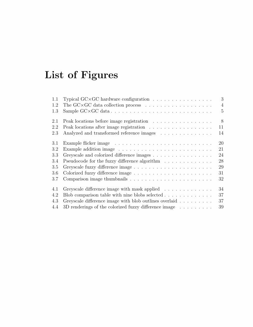
List of Figures
1.1 Typical GC×GC hardware configuration . . . . . . . . . . . . . . . . 31.2 The GC×GC data collection process . . . . . . . . . . . . . . . . . . 41.3 Sample GC×GC data . . . . . . . . . . . . . . . . . . . . . . . . . . . 5
2.1 Peak locations before image registration . . . . . . . . . . . . . . . . 82.2 Peak locations after image registration . . . . . . . . . . . . . . . . . 112.3 Analyzed and transformed reference images . . . . . . . . . . . . . . 14
3.1 Example flicker image . . . . . . . . . . . . . . . . . . . . . . . . . . 203.2 Example addition image . . . . . . . . . . . . . . . . . . . . . . . . . 213.3 Greyscale and colorized difference images . . . . . . . . . . . . . . . . 243.4 Pseudocode for the fuzzy difference algorithm . . . . . . . . . . . . . 283.5 Greyscale fuzzy difference image . . . . . . . . . . . . . . . . . . . . . 293.6 Colorized fuzzy difference image . . . . . . . . . . . . . . . . . . . . . 313.7 Comparison image thumbnails . . . . . . . . . . . . . . . . . . . . . . 32
4.1 Greyscale difference image with mask applied . . . . . . . . . . . . . 344.2 Blob comparison table with nine blobs selected . . . . . . . . . . . . . 374.3 Greyscale difference image with blob outlines overlaid . . . . . . . . . 374.4 3D renderings of the colorized fuzzy difference image . . . . . . . . . 39

List of Tables
2.1 MSE for both blob selection algorithms . . . . . . . . . . . . . . . . . 13
4.1 Available image mask selections . . . . . . . . . . . . . . . . . . . . . 354.2 Blob features displayed in the tabular comparison . . . . . . . . . . . 36

1
Chapter 1
Introduction
The history of two-dimensional gas chromatography dates back to the 1960’s.[3] With
the introduction of comprehensive two-dimensional gas chromatography (GC×GC)
in the early-1990’s,[11] the ability to separate large numbers of chemicals took a huge
leap forward, and the use of this technology for real-world applications has grown
quickly. As GC×GC datasets have grown both more complex and more heavily used,
the need to analyze these datasets and compare the results of multiple datasets has
become more apparent.[20] In fact, Mondello et al. suggested in 2002 that the lack
of good analysis software was perhaps the most significant obstacle to overcome in
order for GC×GC to become more widely accepted.[12]
The data generated by GC×GC is typically represented as a two-dimensional
image of scalar values. Therefore, generic image processing techniques for change
detection may be applied as elementary first steps toward detection of similarities
and differences between two datasets. Several of these techniques are described in
Section 1.2. However, post-processing of individual images with software such as
GC Image[16] can extract a large amount of information about the dataset from
the image and store it as metadata along with the image data. By making use of
2
this metadata and by modifying generic image processing techniques to work better
with the specific types of images produced by GC×GC, an analyst’s ability to detect
similarities and differences between two datasets can be significantly improved.
1.1 Dataset Details
Comprehensive two-dimensional gas chromatography is a recent extension of the well-
established field of one-dimensional gas chromatography. Compared with the one-
dimensional form, GC×GC increases the peak separation capacity by an order of mag-
nitude and can readily distinguish several thousand unique chemical compounds.[2]
GC×GC is performed by taking one GC column and appending to it a second GC
column having retention characteristics which are significantly different than those
of the first column. The two columns are joined by a modulator which traps the
chemicals as they are eluted from the first column and periodically injects them into
the second column. A detector is placed at the end of the second column to measure
and periodically report the concentration and/or other measures of chemicals being
eluted.[12] A diagram of the basic hardware configuration is shown in Figure 1.1.
While the first column typically takes many minutes or hours to process the entire
chemical sample, the second column usually requires only a few seconds. Ideally, the
modulator between the columns is timed so that the entire effluent exits the second
column before the next batch is released into it.[2] A detector running at a typical
sampling frequency of 100 Hz is able to make several hundred distinct measurements
for each pass through the second column, and there are usually several hundred such
passes required before all chemicals are eluted from the first column.
The raw data collected by a flame-ionization detector (FID) is multiplied by a
constant gain coefficient to produce a one-dimensional stream of floating point values

3
Figure 1.1: Typical GC×GC hardware configuration
indicating the concentration of chemicals detected during each interval while exiting
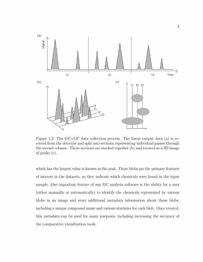
the second column. To transform the data into a two-dimensional image, the raw
data stream is divided into sections, with each section representing the data collected
during one pass through the second column. The sections are stacked together, one
per row, to form a two-dimensional image. This procedure is demonstrated in Fig-
ure 1.2. The dimensions of the resulting image can be measured either in pixels (the
number of measurement intervals of the detector) or in the time required for the given
pixel to elute from each GC column.[8]
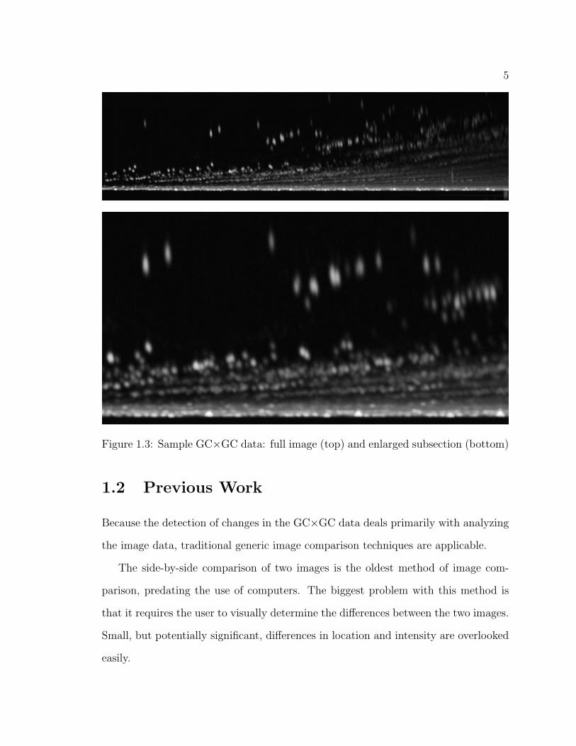
The resulting GC×GC FID images vary greatly in size depending on the equip-
ment parameters of each run, ranging from fewer than 50x500 pixels to more than
1000x5000 pixels. These images contain achromatic intensities, which allows the use
of any desired color scheme in order to assist in visualization. Prior to further auto-
mated analysis of these images, basic post-processing generally is performed on these
images to perform baseline flattening and remove undesirable artifacts such as the
solvent front.[20] Portions of a sample dataset are shown in Figure 1.3.
The GC×GC image data is comprised primarily of a large background area with
small pixel values. Scattered throughout the image are small clusters of pixels with
larger values, known as blobs, which represent higher concentrations of chemicals
emerging from the GC×GC equipment at a particular time. In each blob, the pixel
4
Figure 1.2: The GC×GC data collection process. The linear output data (a) is re-ceived from the detector and split into sections representing individual passes throughthe second column. Those sections are stacked together (b) and treated as a 2D imageof peaks (c).
which has the largest value is known as the peak. These blobs are the primary features
of interest in the datasets, as they indicate which chemicals were found in the input
sample. One important feature of any GC analysis software is the ability for a user
(either manually or automatically) to identify the chemicals represented by various
blobs in an image and store additional metadata information about those blobs,
including a unique compound name and various statistics for each blob. Once created,
this metadata can be used for many purposes, including increasing the accuracy of
the comparative visualization tools.
5
Figure 1.3: Sample GC×GC data: full image (top) and enlarged subsection (bottom)
1.2 Previous Work
Because the detection of changes in the GC×GC data deals primarily with analyzing
the image data, traditional generic image comparison techniques are applicable.
The side-by-side comparison of two images is the oldest method of image com-
parison, predating the use of computers. The biggest problem with this method is
that it requires the user to visually determine the differences between the two images.
Small, but potentially significant, differences in location and intensity are overlooked
easily.

6
With the advent of digital images and graphical computer displays, one of the
earliest methods employed was to subtract the individual pixel values of one image
from the corresponding pixel values in the other image in order to form a difference
image (or subtraction image) that contains only the differences between them.[7] Kun-
zel modified this technique by using the difference image to determine the hue of the
image, while the intensity was determined by the pixel value of one of the original
images.[9]
The three-band nature of RGB color images lends itself to another simple com-
parison technique known as an addition image, where two or three greyscale images
are combined to produce a color image. One image is used as the red band, another
is used as the green band, and another (if desired) is used to form the blue band.
The intensity of each pixel in the output image will be similar to that of the largest
input value. The hue of each pixel will be determined by the combination of the three
input pixel values in the RGB color space.[19]
Another method of image comparison is to use a flicker image, where two images
are alternately displayed in the same location on the screen and the user can rapidly
switch between them.[10] Although the identification of differences is still left to the
user, the fact that both images occupy the same display space makes these differences
much more obvious.
Although these basic techniques work reasonably well for detecting changes in
generic images, the use of blob metadata and other image characteristics specific to
GC×GC allows for improvement in comparison accuracy and ease of analysis.
7
Chapter 2
Dataset Preprocessing
Most GC×GC analysis tasks operate on a single dataset. When comparing two
images, the dataset currently selected for analysis is known as the analyzed image.
Within the image comparison process, a second image is selected for comparison
against the primary (analyzed) image. This second image is termed the reference
image.
Before any comparison can be performed, the data in the reference image must
be transformed so that corresponding features in the two images occupy the same
pixel location. The magnitude of the pixel values in the reference image must also be
scaled so that pixels representing identical physical characteristics will have the same
pixel value in the two images. These two steps are critical to the software’s ability to
deemphasize common features and emphasize only the real differences.
2.1 Data Transformation
Due to the nature of the GC×GC process, two samples of the same mixture pro-
duce datasets that have peaks which are in slightly different locations (indicating
that they were eluted at slightly different times) and which have slightly different
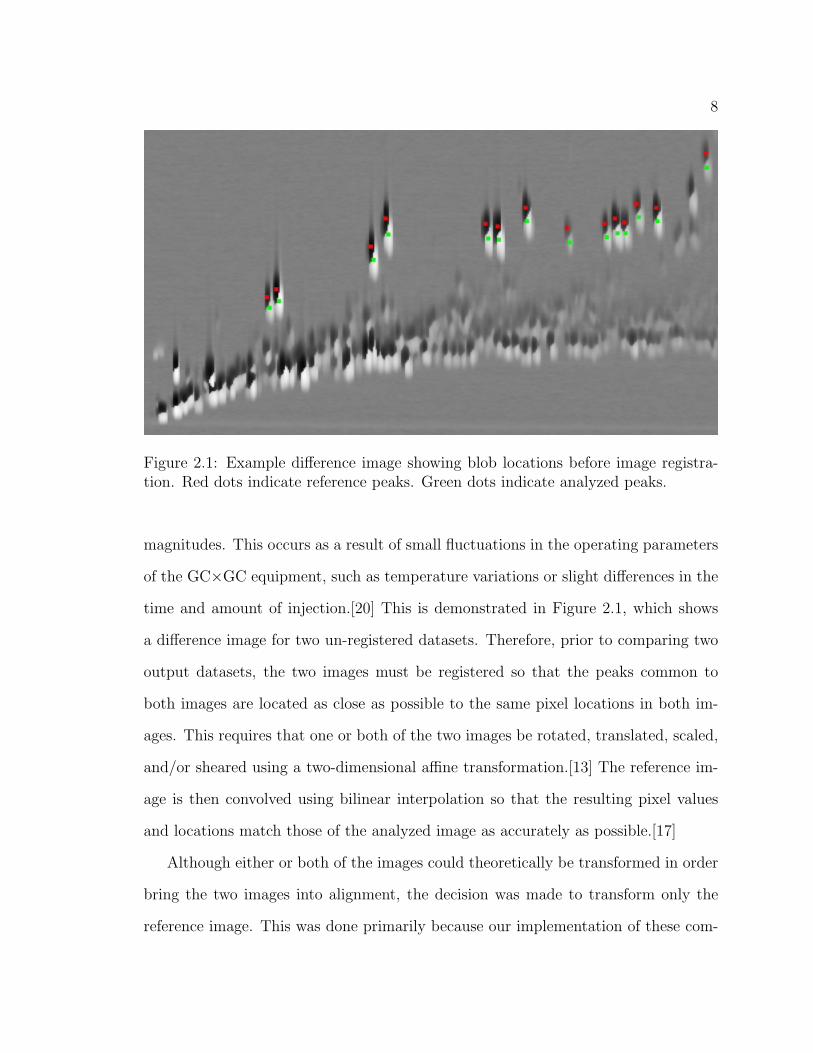
8
Figure 2.1: Example difference image showing blob locations before image registra-tion. Red dots indicate reference peaks. Green dots indicate analyzed peaks.
magnitudes. This occurs as a result of small fluctuations in the operating parameters
of the GC×GC equipment, such as temperature variations or slight differences in the
time and amount of injection.[20] This is demonstrated in Figure 2.1, which shows
a difference image for two un-registered datasets. Therefore, prior to comparing two
output datasets, the two images must be registered so that the peaks common to
both images are located as close as possible to the same pixel locations in both im-
ages. This requires that one or both of the two images be rotated, translated, scaled,
and/or sheared using a two-dimensional affine transformation.[13] The reference im-
age is then convolved using bilinear interpolation so that the resulting pixel values
and locations match those of the analyzed image as accurately as possible.[17]
Although either or both of the images could theoretically be transformed in order
bring the two images into alignment, the decision was made to transform only the
reference image. This was done primarily because our implementation of these com-

9
parative visualization techniques is part of a larger software package for analysis of
GC×GC data.[16] The analyzed image is the one that has previously been selected
for analysis (hence the name). The reference image is selected only for comparison
within this part of the application. Keeping the analyzed image in its original ori-
entation provides a more intuitive environment for the analyst using this software,
because the user is most likely already familiar with the image in that form.
To determine the transformation that maps the reference image onto the analyzed
image, a least-squares fit algorithm is run on the peak locations of a subset of the
blobs that exist in both images. The selection of this subset is discussed below.
The peak location of each blob is determined by GC×GC analysis software prior to
the comparison process and stored as metadata along with the GC×GC image data.
The blobs are matched between the two images based on the compound name (if
any) assigned to each blob. First, unnamed blobs are eliminated from consideration.
Next, blobs which share the same name with another blob in the same dataset are
eliminated from consideration. Such blobs occur infrequently, and usually as a result
of operator error when assigning the names. Finally, for each remaining blob in
the analyzed image, an exhaustive search is performed within the remaining blobs
from the reference image for a blob with the same name. If one is found, that
pair of blobs is added to a list of blobs to be used in the least-squares fit. The
least-squares fit algorithm determines the optimal transform which, when applied to
the pixel coordinates of each peak from the reference image, minimizes the sum of
the squared Euclidean distances between the coordinates of each reference peak and
the coordinates of the corresponding analyzed peak.[4] The squared error sum E is
computed as
E =∑
b∈ blob list
(xab− xrb
)2 + (yab− yrb
)2
where ab and rb are the corresponding analyzed and reference peaks for blob b, and

10
x and y are the pixel coordinates for the specified peak.
Frequently, there will be several blobs in the datasets that, although identified
as the same compound, will be located in significantly different positions even after
the reference image has been transformed. Pairs of peaks that are excessively mis-
matched between the two images tend to reduce the accuracy of the transformation.
To compensate for this, two different approaches were developed.
In the first approach, a two-stage algorithm is used when computing the least-
squares fit. After the first transform is computed from all shared peaks, the peak
locations from the reference image are transformed, and the Euclidean distance is
computed between the analyzed image peaks and the transformed corresponding ref-
erence image peaks. Those peaks whose distances are in the largest 25% are removed
from consideration (while ensuring that at least three peaks are retained), and the
least-squares fit is recomputed on the remaining peaks to obtain the final affine trans-
formation. This simple modification to the basic algorithm assumes that no more than
25% of the blobs will be grossly mis-aligned and that the remaining 75% are sufficient
to produce a good transformation. This has proven to work well in practice. The
results of this elimination process are demonstrated in Figure 2.2.
A second, iterative approach to pruning excessively mismatched peaks also was
developed. At each iteration, a least-squares fit is first computed using the current
list of peaks common to both images. The peak locations from the reference image
are then transformed, and the Euclidean distance is computed between each analyzed
peak and the corresponding transformed reference peak. The peak with the largest
distance is then compared to a predetermined threshold value. If the distance is above
the threshold, that peak is removed from the list and the process is repeated using
the remaining peaks. If the distance is below the threshold, then the loop terminates
and the last transform is used for the rest of the comparative visualization process.
11
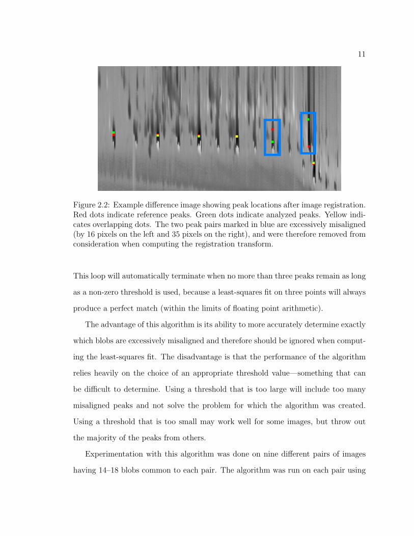
Figure 2.2: Example difference image showing peak locations after image registration.Red dots indicate reference peaks. Green dots indicate analyzed peaks. Yellow indi-cates overlapping dots. The two peak pairs marked in blue are excessively misaligned(by 16 pixels on the left and 35 pixels on the right), and were therefore removed fromconsideration when computing the registration transform.
This loop will automatically terminate when no more than three peaks remain as long
as a non-zero threshold is used, because a least-squares fit on three points will always
produce a perfect match (within the limits of floating point arithmetic).
The advantage of this algorithm is its ability to more accurately determine exactly
which blobs are excessively misaligned and therefore should be ignored when comput-
ing the least-squares fit. The disadvantage is that the performance of the algorithm
relies heavily on the choice of an appropriate threshold value—something that can
be difficult to determine. Using a threshold that is too large will include too many
misaligned peaks and not solve the problem for which the algorithm was created.
Using a threshold that is too small may work well for some images, but throw out
the majority of the peaks from others.
Experimentation with this algorithm was done on nine different pairs of images
having 14–18 blobs common to each pair. The algorithm was run on each pair using
12
thresholds varying from 3 to 20 pixels. For each threshold, the mean squared error
(MSE) was computed for each of the image pairs. The MSE is defined as
MSE =1
N
∑all pixels
(va − vr)2
where N is the number of pixels in each image, va is the pixel value from the analyzed
image, and vr is the corresponding pixel value from the reference image.[1]
The threshold which produced the smallest MSE varied greatly (from 3 to 20
pixels) even within this small test set, although a threshold of 5 most frequently
produced the best results. The results of these tests are presented in Table 2.1 on
page 13. The MSE also was computed by applying the aforementioned “drop 25%”
algorithm to each of the image pairs. The “drop 25%” MSE was sometimes much
smaller than, sometimes much larger than, and sometimes comparable to the best
MSE produced by the iterative algorithm. Regardless of the threshold used, neither
of the algorithms performed consistently better or worse than the other. Optimal
performance of the iterative algorithm relies on choosing the appropriate threshold,
and this threshold appears to vary widely even among similar datasets. This makes
the algorithm difficult to use effectively. Because of this, the iterative algorithm was
set aside pending further research, and the “drop 25%” algorithm was chosen for use
in this application.
Once an acceptable transform has been generated, the reference image and all
associated blob metadata is transformed, and a new working copy of the reference
image is created that contains only those pixels whose new locations fall inside the
bounds of the analyzed image. This working image is the same size as the analyzed
image. Those pixels in the new working copy which were beyond the bounds of
the original, unmodified reference image are masked out and do not affect further

13
Selection MSE for each image pairAlgorithm G1P1 G1P2 G1P3 G1P4Drop 25% 38.238 81.462 131.129 142.430Peaks Retained 13/18 13/18 13/18 13/18Threshold 3 28.780 56.141 93.663 49.527Peaks Retained 17/18 16/18 15/18 15/18Threshold 5 28.780 56.421 56.269 33.907Peaks Retained 17/18 17/18 17/18 17/18
Selection MSE for each image pairAlgorithm G2P1 G2P2 G2P3 G2P4 G2P5Drop 25% 1678083 2714662 1600533 3832121 2068510Peaks Retained 10/14 10/14 10/14 10/14 10/14Threshold 3 968255 3192925 3533956 3288412 1991317Peaks Retained 7/14 8/14 5/14 5/14 6/14Threshold 5 1115525 3065092 3083609 3288412 2076938Peaks Retained 10/14 9/14 7/14 5/14 8/14Threshold 7 1115525 3212437 3145972 4726396 2068510Peaks Retained 10/14 10/14 8/14 8/14 10/14Threshold 10 1115525 3564295 3155536 4659423 2068510Peaks Retained 10/14 12/14 9/14 9/14 10/14Threshold 15 1684530 3564295 3241191 4593703 2437782Peaks Retained 11/14 12/14 10/14 10/14 11/14Threshold 20 1685073 3564295 2650232 4417996 2600084Peaks Retained 12/14 12/14 13/14 11/14 12/14
Table 2.1: MSE and number of peaks retained for both blob selection algorithms ontwo groups of image pairs. The images within each group were created from differentruns on the same chemical sample and were therefore very similar. For the first group,thresholds from 5–20 yielded identical results.
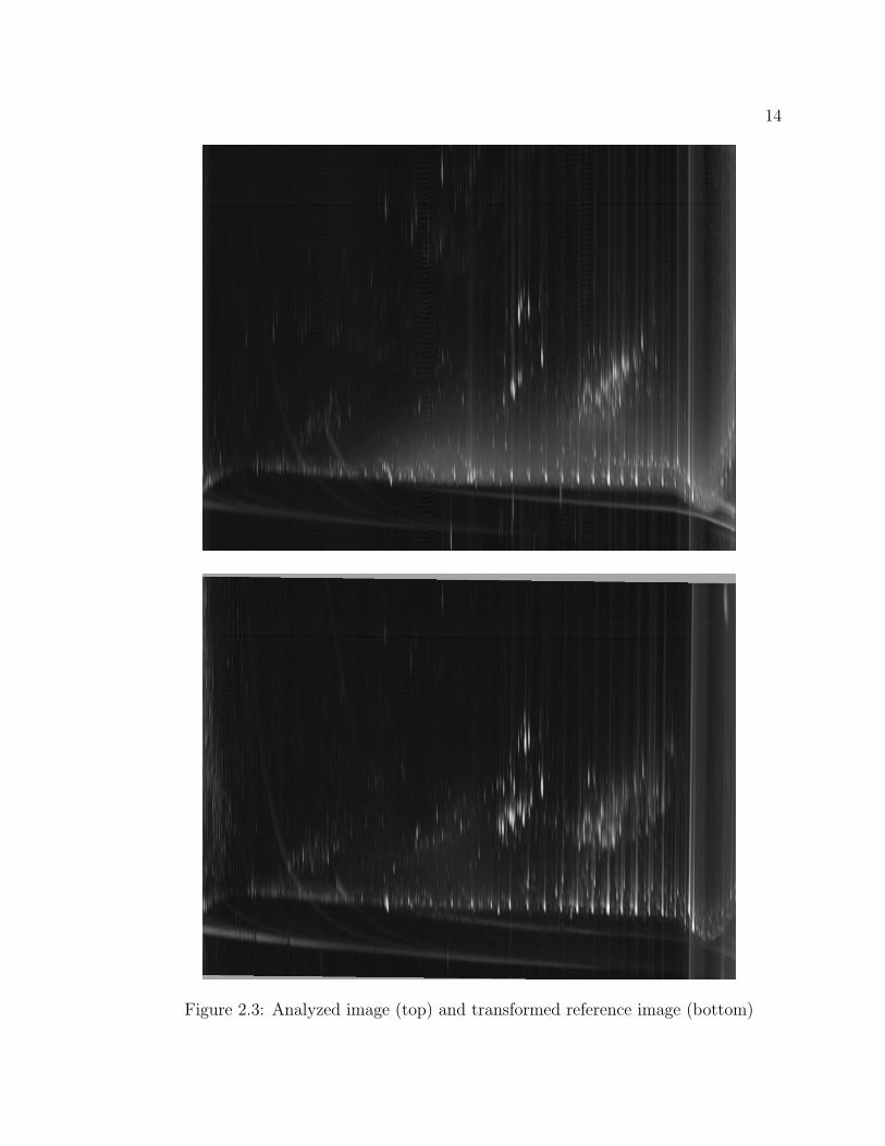
processing. These pixels are displayed as grey blocks at the top and bottom of the
reference image in Figure 2.3 on page 14. From this point forward in the image
comparison process, all mentions of the reference image refer to this transformed
working copy, not to the original reference image.
14
Figure 2.3: Analyzed image (top) and transformed reference image (bottom)
15
2.2 Data Normalization
Due to the nature of GC×GC, even when two tests are performed on two identical
samples, the concentrations of each compound appearing in the output data will
differ somewhat. These differences in pixel values, if left unaltered, would incorrectly
indicate differences in the amount of each compound when no difference actually
existed. To avoid this problem, the reference image is normalized by applying a
linear scale factor to every pixel value as well as to the relevant features in the
blob metadata (such as the pre-computed volume of each blob). This makes most
corresponding pixel values approximately equal between the two images and makes
differences in peak height more apparent.
This normalization factor is computed using a subset of the blobs which are com-
mon to both the analyzed and the reference image. The volume Vb of blob b is defined
as the sum of the values vp for all pixels p contained in the blob.
Vb =∑p∈ b
vp
The normalization scale factor S is then defined as the sum of the blob volumes from
the analyzed image divided by the sum of the blob volumes from the reference image.
S =
∑b∈analyzed Vb∑b∈reference Vb
Finally, the value vp of each pixel p in the reference image is multiplied by the scale
factor.
v′p = vp × S, ∀p ∈ reference image
The collection of blobs used for the normalization process is determined using one
of three methods. If there are any internal standard blobs defined in the two images,

16
those blobs are used for normalization. An internal standard is a precise amount of a
certain compound that is inserted into the original input sample. It is used specifically
to aid in normalization of the data values, and is not part of the unknown sample
being analyzed. If no internal standards are present, then all pairs of blobs which
are marked as “included” by the user are used for normalization. The included flag
is a feature of the GC Image software that allows the user to indicate the desire to
include this blob’s individual information in certain processing steps. If there are no
internal standards or included blobs, then all blobs common to both images are used
for normalization.
If internal standards are present, they are trusted implicitly, because they were
introduced for this very purpose. However, if no internal standards are present, a
small percentage of the shared blobs will sometimes be dramatically larger in one
image than the other. Not only will such blobs skew the normalization factor for
all blobs, but a biased normalization factor will help to hide blobs of significantly
different heights which the user is likely trying to identify. This problem is solved
by applying the same theory used to improve the least-squares fit transformation.
Specifically, an initial scale factor is computed using all blobs in the appropriate
collection. For each blob, the difference in peak height between the two images is
computed. Those blobs whose difference magnitudes are in the largest 25% (rounded
down to the nearest blob) are removed from further consideration, and the final
normalization factor is computed using the remaining blobs. Dropping those blobs
with the largest raw difference values rather than those with the largest percentage
difference usually means dropping the blobs with the largest volumes and recomputing
the scale using the smaller blobs. This reduces the likelihood of the scale factor being
dominated by one or two enormous blobs, which would have happened in at least one
series of datasets used for testing.
17
Chapter 3
Image-Based Comparison Methods
The focus of this research was to enhance generic image comparison techniques and
develop new techniques that allow the user to more accurately and easily compare
and contrast the two GC×GC datasets. The following sections detail each of the
implemented comparison methods. Three well-known techniques are discussed as
well as a new “fuzzy difference” comparison method and a new colorization scheme
that allows more information to be conveyed than does a standard greyscale difference
image. These comparison methods are illustrated using side by side thumbnails in
Figure 3.7 on page 32.
3.1 Pre-existing Comparison Methods
3.1.1 Flicker
The flicker comparison method alternately displays each image in the same location
on the screen, allowing the user to visually determine where the significant differences

18
lie. Because the original images contain floating point pixel values with a variable
range, the pixel values are scaled into an 8-bit greyscale image with pixel values in
the 0–255 range for display to the screen. Darker pixels represent smaller values and
lighter pixels represent larger values. Pixel values from both images are normalized
using the same scale factor so that each original pixel value will map to the same
display value regardless of which image is currently displayed.
A special formula is used when scaling the floating point pixel values into the
8-bit integer range for display. Because the GC×GC data typically has blobs with
peak values of 100 or larger (sometimes over 10,000) next to off-peak values of less
than 2, a straight linear scale would result in sharply defined peaks with little or no
definition among the lower values. In order to increase the resolution at lower pixel
values, the raw pixel values are shifted so that the minimum value is 1.0, then the
natural logarithm of the adjusted value is computed, then this value is raised to a
user-selected power (typically around 0.7). Specifically, for each power q and value
vp at pixel p,
vmin = min∀p
vp (3.1)
v′p = (ln(vp − vmin + 1))q (3.2)
The resulting value v′p is then scaled linearly into the appropriate value range.
The log result is raised to a power in order to increase the resolution at lower pixel
values further than was possible using only the natural log. It also allows the analyst
more control over the visual significance of the lower values. Equation 3.2 is used
throughout the image-based comparison methods discussed here whenever floating
point data must be scaled into a non-native range.
After equation 3.2 is applied to each pixel value in both images, the minimum and
maximum values v′min and v′max at any pixel location p in either the analyzed (a) or

19
reference (r) image are determined using
v′min = min∀p
(min(|a′p|, |r′p|)) (3.3)
v′max = max∀p
(max(|a′p|, |r′p|)) (3.4)
Finally, the new 8-bit value v′′p is computed as
v′′p =(v′p − v′min)
v′max
× 255 (3.5)
An example flicker image is shown in Figure 3.1 on page 20.
The user may manually switch between the analyzed and reference images by
clicking a button in the control window, or the software can cycle between the images
automatically at a time interval specified by the user.
The flicker comparison is a useful tool for quickly comparing the shape and location
of various blobs. However, the human eye’s poor responsiveness to small changes in
greyscale pixel intensities in areas of geographically rapid change—such as the blob
peaks—makes accurate comparison of peak heights difficult.[7]
3.1.2 Addition
Another popular method for comparing images is to create what is known as an
addition image. To do this, both the original analyzed and reference images are
converted to 8-bit greyscale images using the same scale factor. The scale factor used
here is the same one used for the individual flicker images detailed in Section 3.1.1
(calculated using equations 3.1 through 3.5).
A 3-band RGB image is then created by using the scaled analyzed image for the
green band and the scaled reference image for the red band. Zeros are used for the

20
Figure 3.1: Example flicker image
21
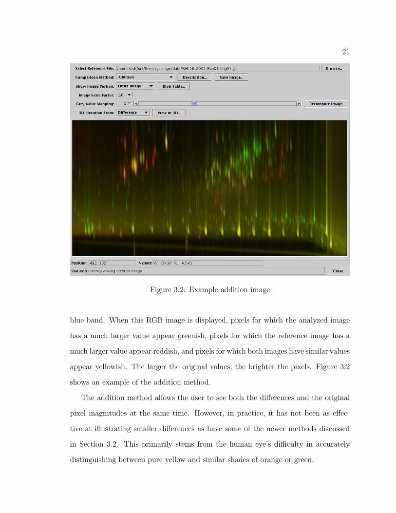
Figure 3.2: Example addition image
blue band. When this RGB image is displayed, pixels for which the analyzed image
has a much larger value appear greenish, pixels for which the reference image has a
much larger value appear reddish, and pixels for which both images have similar values
appear yellowish. The larger the original values, the brighter the pixels. Figure 3.2
shows an example of the addition method.
The addition method allows the user to see both the differences and the original
pixel magnitudes at the same time. However, in practice, it has not been as effec-
tive at illustrating smaller differences as have some of the newer methods discussed
in Section 3.2. This primarily stems from the human eye’s difficulty in accurately
distinguishing between pure yellow and similar shades of orange or green.

22
3.1.3 Greyscale Difference
One of the best known and most commonly used methods of comparing two images
is to subtract the individual pixel values of one image from the corresponding pixel
values in the other image in order to form a difference image that contains only the
differences between the two input images. In our GC×GC application, the reference
image is subtracted from the analyzed image, so positive difference values indicate
that the analyzed image had a larger value, while negative difference values indicate
that the reference image was larger. At each pixel location p,
∆p = ap − rp (3.6)
where ap is the analyzed pixel value, rp is the reference pixel value, and ∆p is the
difference between them.
The floating point difference image is converted into an 8-bit greyscale image for
display. Medium grey (display value 128) is used to represent zero difference, with
positive values being brighter (display values 129 to 255) and negative values being
darker (display values 1 to 127). The larger the magnitude of the difference, the closer
the displayed pixel will be to white or black. The same scale factor is used for both
positive and negative values, so the resulting 8-bit image will include either value
1 or 255, but perhaps not both. Pixel value 0 is reserved to indicate pixels which
are outside the bounds of the reference image after it was transformed and therefore
cannot be used for comparison.
Prior to scaling the difference values (∆p) for display, they are processed using
equations 3.1 and 3.2. When used to pre-process pixel values from a difference image
(including those produced by the new difference methods discussed in Section 3.2),
the absolute value of vp is used in those equations, and the sign of the original vp
23
is assigned to the resulting v′p in equation 3.2. This ensures that both positive and
negative differences are scaled consistently regardless of the sign of the difference.
The value v′p is then renamed to ∆′p (representing the modified difference value
at pixel p) and scaled linearly into the appropriate value range using the following
equations. If ∆′max is the maximum magnitude of any floating point value ∆′
p, the
scaled display value ∆′′p is computed as
∆′max = max
∀p|∆′
p| (3.7)
∆′′p =
∆′p × 127
∆′max
+ 128 (3.8)
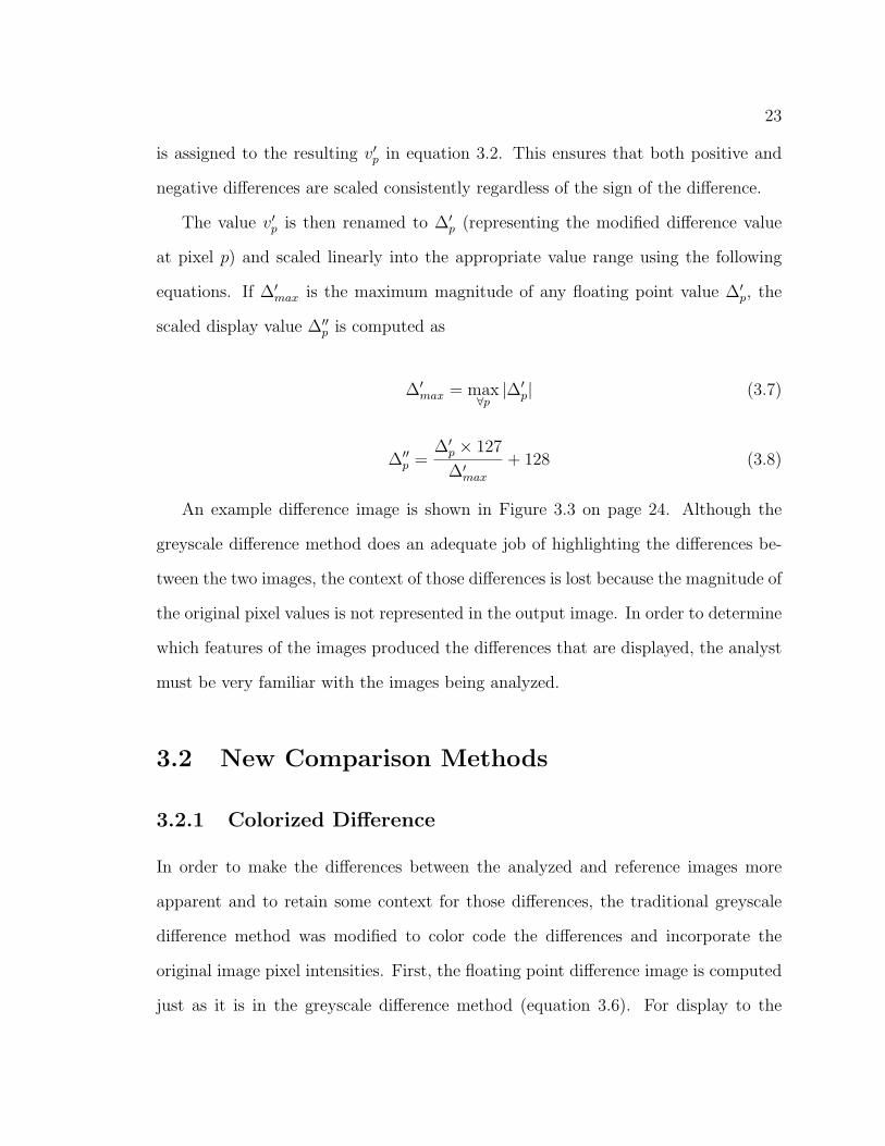
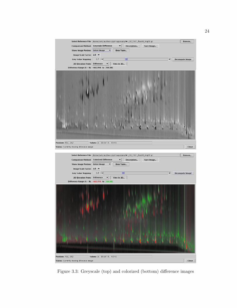
An example difference image is shown in Figure 3.3 on page 24. Although the
greyscale difference method does an adequate job of highlighting the differences be-
tween the two images, the context of those differences is lost because the magnitude of
the original pixel values is not represented in the output image. In order to determine
which features of the images produced the differences that are displayed, the analyst
must be very familiar with the images being analyzed.
3.2 New Comparison Methods
3.2.1 Colorized Difference
In order to make the differences between the analyzed and reference images more
apparent and to retain some context for those differences, the traditional greyscale
difference method was modified to color code the differences and incorporate the
original image pixel intensities. First, the floating point difference image is computed
just as it is in the greyscale difference method (equation 3.6). For display to the
24
Figure 3.3: Greyscale (top) and colorized (bottom) difference images

25
screen, the raw difference image is converted into a 24-bit RGB color image (three
separate bands of 8-bit integers). The color computation is done in the Hue-Intensity-
Saturation (HIS) color space.[6] The hue component of each pixel is set to pure green
if the analyzed pixel value is larger or pure red if the reference pixel value is larger.
The intensity component ip of each pixel p is the maximum of the original analyzed
and reference pixel values ap and rp, scaled to fit into the 0–1.0 range. Equation 3.2
is first applied to ap and rp, then
ip =max(|a′p|, |r′p|)
v′max
(3.9)
using v′max from equation 3.4.
The saturation component sp is the magnitude of the raw difference value, scaled
to fit into the 0–1.0 range. Equation 3.2 is first applied to each ∆p as described in
Section 3.1.3, then
sp =|∆′
p|∆′
max
(3.10)
using ∆′max from equation 3.7.
After the hue, intensity, and saturation components are calculated for each pixel,
they are converted to the RGB color space and stored in a 24-bit image for display
to the screen.
The resulting color image shows lighter pixels where either of the original images
had larger values and darker pixels where both of the original images had smaller val-
ues, thereby retaining the context for the differences that was lacking in the greyscale
difference method. Pixels that had approximately equal values in both original im-
ages will appear greyish, while pixels for which there was a large difference will have
bolder colors. This allows the user to see not only where the greatest differences lie
between the two images, but also where those differences are located in relation to

26
the blob peaks in the images. For comparison, the colorized and greyscale difference
images are shown side by side in Figure 3.3 on page 24.
This colorization method is inspired by the work of Kunzel, who suggested using
the ARgYb color space to display the original pixel values via the intensity component
(A) and the differences among three radiographs via the color components (Rg and
Yb).[9] Thanks to the use of the HIS color space instead of ARgYb, our algorithm is
not only computationally simpler, but also allows the use of a wider range of color
saturation than does Kunzel’s.
3.2.2 Greyscale Fuzzy Difference
In practice, the most common difference between the analyzed and reference images
comes from blob peaks that are misaligned by only a few pixels, but otherwise have
very similar values. Minimizing the effect of these slightly misaligned peaks is impor-
tant because they are not the differences in which the user is typically most interested.
Precise alignment using piecewise or non-rigid convolution techniques is sometimes
problematic with the GC×GC data because most of the transformation control points
(shared, named peaks) may frequently lie along a nearly straight line. A better com-
parison method would reduce the differences between such similar peaks while still
displaying large differences for peaks that have either grown or moved significantly
between the two images. The greyscale and colorized fuzzy difference comparison
methods accomplish these goals.
To compute the fuzzy difference between the two images, the user specifies the
size of a rectangular window. Typical window sizes range from 3x5 to 7x15. The
difference value at each pixel in the output image is computed using a three-step
process. Two intermediate difference images are first computed as follows. For each
pixel location, the difference is computed between that pixel value in the analyzed
27
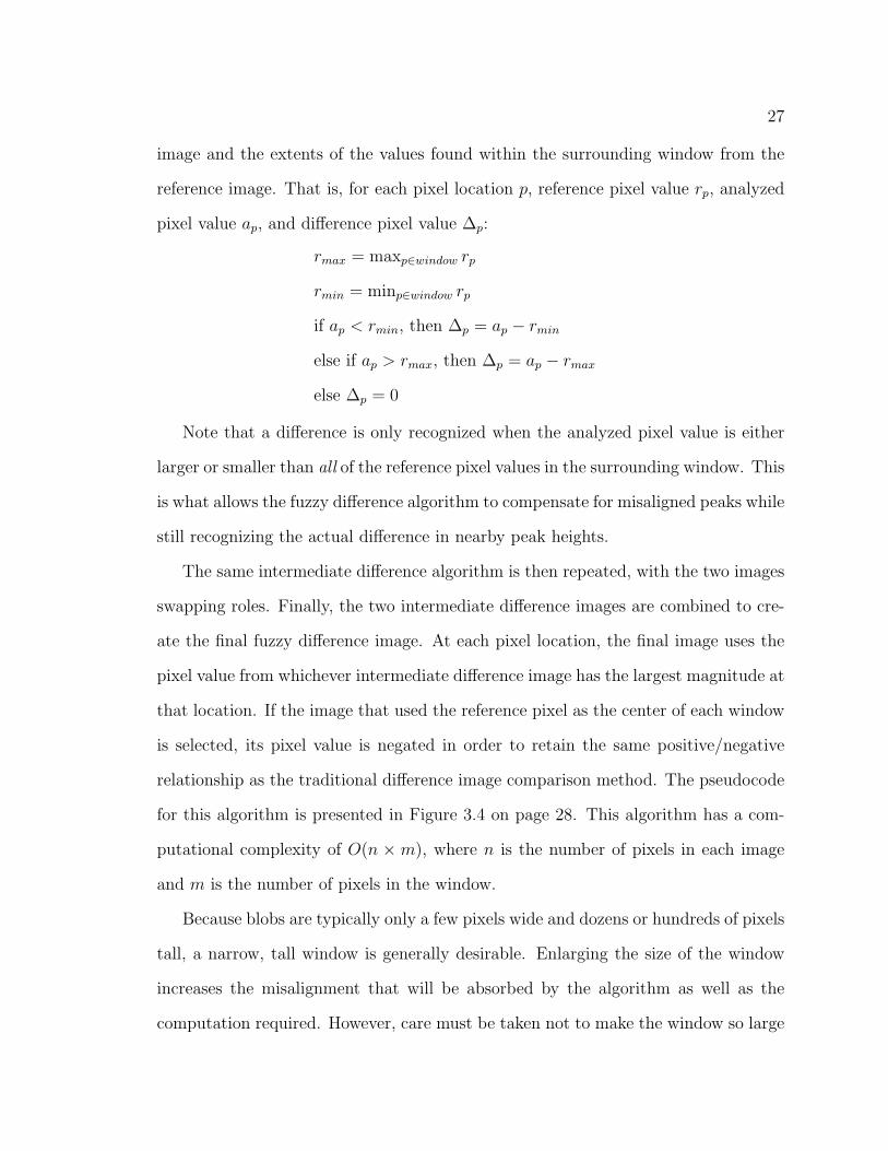
image and the extents of the values found within the surrounding window from the
reference image. That is, for each pixel location p, reference pixel value rp, analyzed
pixel value ap, and difference pixel value ∆p:
rmax = maxp∈window rp
rmin = minp∈window rp
if ap < rmin, then ∆p = ap − rmin
else if ap > rmax, then ∆p = ap − rmax
else ∆p = 0
Note that a difference is only recognized when the analyzed pixel value is either
larger or smaller than all of the reference pixel values in the surrounding window. This
is what allows the fuzzy difference algorithm to compensate for misaligned peaks while
still recognizing the actual difference in nearby peak heights.
The same intermediate difference algorithm is then repeated, with the two images
swapping roles. Finally, the two intermediate difference images are combined to cre-
ate the final fuzzy difference image. At each pixel location, the final image uses the
pixel value from whichever intermediate difference image has the largest magnitude at
that location. If the image that used the reference pixel as the center of each window
is selected, its pixel value is negated in order to retain the same positive/negative
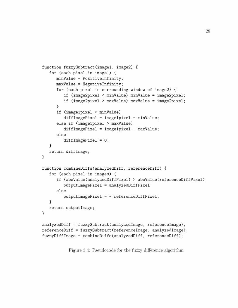
relationship as the traditional difference image comparison method. The pseudocode
for this algorithm is presented in Figure 3.4 on page 28. This algorithm has a com-
putational complexity of O(n × m), where n is the number of pixels in each image
and m is the number of pixels in the window.
Because blobs are typically only a few pixels wide and dozens or hundreds of pixels
tall, a narrow, tall window is generally desirable. Enlarging the size of the window
increases the misalignment that will be absorbed by the algorithm as well as the
computation required. However, care must be taken not to make the window so large
28
function fuzzySubtract(image1, image2) {
for (each pixel in image1) {
minValue = PositiveInfinity;
maxValue = NegativeInfinity;
for (each pixel in surrounding window of image2) {
if (image2pixel < minValue) minValue = image2pixel;
if (image2pixel > maxValue) maxValue = image2pixel;
}
if (image1pixel < minValue)
diffImagePixel = image1pixel - minValue;
else if (image1pixel > maxValue)
diffImagePixel = image1pixel - maxValue;
else
diffImagePixel = 0;
}
return diffImage;
}
function combineDiffs(analyzedDiff, referenceDiff) {
for (each pixel in images) {
if (absValue(analyzedDiffPixel) > absValue(referenceDiffPixel)
outputImagePixel = analyzedDiffPixel;
else
outputImagePixel = - referenceDiffPixel;
}
return outputImage;
}
analyzedDiff = fuzzySubtract(analyzedImage, referenceImage);
referenceDiff = fuzzySubtract(referenceImage, analyzedImage);
fuzzyDiffImage = combineDiffs(analyzedDiff, referenceDiff);
Figure 3.4: Pseudocode for the fuzzy difference algorithm
29
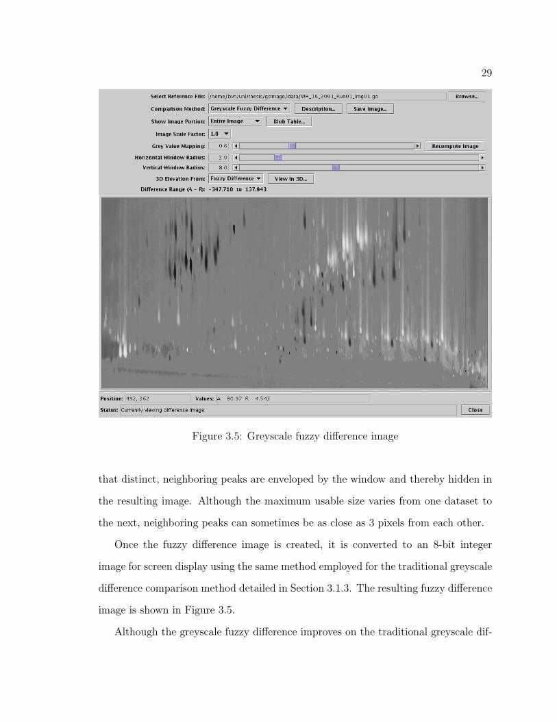
Figure 3.5: Greyscale fuzzy difference image
that distinct, neighboring peaks are enveloped by the window and thereby hidden in
the resulting image. Although the maximum usable size varies from one dataset to
the next, neighboring peaks can sometimes be as close as 3 pixels from each other.
Once the fuzzy difference image is created, it is converted to an 8-bit integer
image for screen display using the same method employed for the traditional greyscale
difference comparison method detailed in Section 3.1.3. The resulting fuzzy difference
image is shown in Figure 3.5.
Although the greyscale fuzzy difference improves on the traditional greyscale dif-

30
ference by removing many of the uninteresting details while retaining the interesting
details, it still suffers from the same major drawback as the traditional greyscale
difference—that it does not show any visible context for the resulting differences
among the surrounding features of the original images.
3.2.3 Colorized Fuzzy Difference
The final comparison method takes the greyscale fuzzy difference algorithm described
in Section 3.2.2 and applies the same colorization algorithm used in the colorized
difference method described in Section 3.2.1, which uses intensity to indicate the
pixel values from the original images and color to indicate the differences between
the two images. An example of the colorized fuzzy difference image can be seen
in Figure 3.6 on page 31. The resulting displayed image shares the benefits that
both of those methods have over the traditional greyscale difference, namely, that it
removes many uninteresting details by compensating for misaligned peaks, and that
it indicates the pixel values from the original images to provide some context for
the difference values. In practice, the colorized fuzzy difference algorithm appears to
effectively highlight the interesting differences in blob peak heights and shapes, even
when peaks are slightly misaligned.

31
Figure 3.6: Colorized fuzzy difference image

32
Figure 3.7: Comparison image thumbnails. Top row: original analyzed image (left),greyscale difference (center), and greyscale fuzzy difference (right). Middle row: orig-inal reference image (left), colorized difference (center), and colorized fuzzy difference(right). Bottom row: addition.

33
Chapter 4
Additional Dataset Analysis
Once the displayable images have been generated for any of the image-based compar-
ison methods, additional operations can be performed on the datasets to enhance the
user’s understanding of the data.
4.1 Masking Images
Although the comparison process attempts to remove uninteresting differences and
highlight interesting ones, the users may want to mask off certain areas of an image
so that comparisons are only displayed for a particular subsection of the image area.
To accomplish this, the image comparison procedure allows the user to mask off a
variety of different areas described in Table 4.1 on page 35. This mask is applied as
the final step after all other preprocessing and comparison image computation has
been performed on the entire image area. Pixels outside the mask’s active area are
displayed as a null value appropriate for the currently selected comparison method.
For example, the addition method would use black, while the greyscale difference
method would use medium grey. Examples of masked and unmasked difference images
are shown in Figure 4.1 on page 34.

34
Figure 4.1: Entire greyscale difference image (top) and the same image with a maskshowing only included blobs (bottom)

35
Mask Type Active Area Displayed
Entire Image The entire imageAll Blobs The area covered by all blobs in either imageIncluded Blobs The area covered by blobs in either image which the user has
designed as “included”Selected Blobs The area covered by blobs in either image which the user has
interactively selectedIncluded Shapes The area covered by shapes marked as “included,” minus any
shapes marked as “excluded”
Table 4.1: Available image mask selections
4.2 Tabular Data
In addition to the image-based comparison methods outlined in Chapter 3, the nu-
merical characteristics of the blobs defined in each GC×GC dataset may be compared
side by side in a blob comparison table. The only blobs displayed in the table are
those which have the same compound name as exactly one blob in the other image.
The features displayed for each blob are listed in Table 4.2 on page 36. For each
feature, the values for the analyzed and reference image are listed side by side in
the table. For those features marked in Table 4.2 with an asterisk (*), the difference
between the feature values of the two images is also listed. To aid in analysis, the
table rows containing the blobs may be ordered using any feature for either image or
any feature difference between the images by clicking the mouse on the header of the
appropriate column. The contents of this table may be saved to a comma-separated,
quoted, ASCII text file for later importation into a variety of spreadsheet or database
applications.
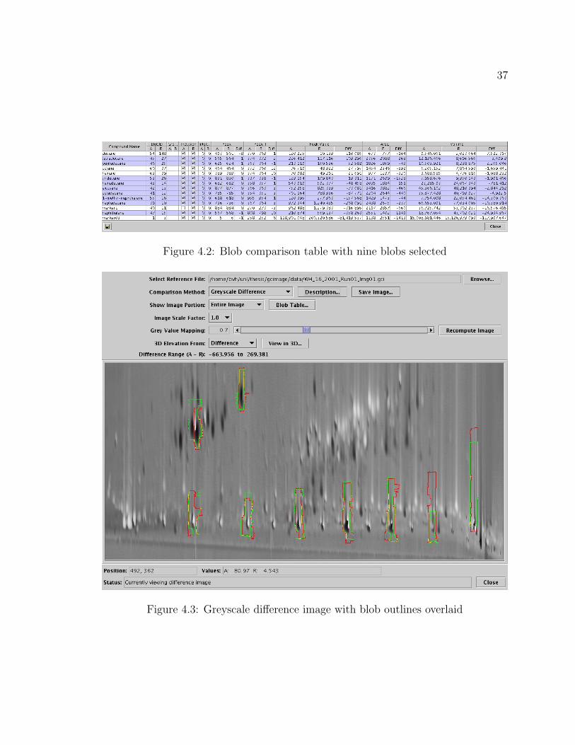
If one or more blobs in the table are selected by clicking the appropriate rows with
the mouse, those rows are highlighted and the outlines of those blobs are drawn on
top of the current comparison image in the image comparison window. The analyzed
blob is outlined in green and the reference blob is outlined in red. This allows the

36
Feature DescriptionID Number Unique identifier for each blob within each datasetGroup Name Name of the group to which this blob belongsInclusion Status Whether or not the blob is marked for inclusionInternal Standard ID number for the associated internal standard blobPeak Location Pixel coordinates of the peak value along each axis *Peak Value The highest pixel value in the blob *Area The number of pixels encompassed by the blob *Volume The sum of all pixel values encompassed by the blob *
Table 4.2: Blob features displayed in the tabular comparison
user to easily locate the blobs of interest; for example, the corresponding blobs with
the largest volume difference. The blob comparison table and a greyscale difference
image with several blobs outlined are shown in Figures 4.2 and 4.3 on page 37.
4.3 Three-Dimensional Visualization
Although the various image-based comparison methods combined with the tabular
data help the user interpret the datasets, it is sometimes helpful to visualize the
GC×GC image data as an elevation map, with blob peaks and background pixels
emulating mountains and valleys. The software allows the user to view the image data
in an interactive, three-dimensional environment. Pixels from one of several image
sources are treated as an elevation map, and the image generated by the currently
selected comparison method is draped over the surface of the elevation map to provide
coloration. The user can then view the data from various distances or viewing angles
and can locate the viewer’s position anywhere in or around the data.
This capability is available for single images in the GC Image package, and was
modified in order to enhance the visualization capabilities of the image comparison
package. If any areas of the comparison image have been masked out or any blob
outlines have been drawn into this image, those changes are transfered into the 3D
37
Figure 4.2: Blob comparison table with nine blobs selected
Figure 4.3: Greyscale difference image with blob outlines overlaid

38
view as well.
For the elevation map, the user may select one of four different images:
• The original analyzed image data.
• The original reference image data (after transformation and normalization).
• An image containing the maximum pixel value at each location from either the
analyzed or reference image.
• The difference image. If either of the fuzzy difference comparison methods is
selected, the fuzzy difference is used. For all other comparison methods, the
traditional difference is used.
Masked areas, if selected, are applied to the elevation map as well, with inactive
pixels having a value of zero. The ability to drape any of the comparison images
over a variety of different elevation maps allows the user great versatility in analyzing
the data. It also allows even the greyscale difference comparisons (traditional or
fuzzy) to be viewed in the context of the original pixel data—something that is not
possible using only a two-dimensional image. Another advantage of the 3D view is
the user’s ability to compare elevation peak heights by viewing the image from the
side and sighting across the tops of the elevation peaks. Sample 3D views are shown
in Figure 4.4 on page 39.

39
Figure 4.4: 3D renderings of the colorized fuzzy difference image draped over themaximum value elevation map
40
Chapter 5
Conclusions and Future Work
Initial reports from GC×GC analysts with the United States Coast Guard Academy
are promising. The registration and normalization methods detailed in Chapter 2 for
matching peak locations and other features of the reference image to the analyzed im-
age are adequate for most analyses. However, there is still room for future work with
the selection of control points or alternate registration algorithms to improve this pro-
cess. Improvements in image registration could reduce the uninteresting differences
generated by the various comparison methods and therefore reduce, but probably
not eliminate, the need for the fuzzy difference algorithms presented in Sections 3.2.2
and 3.2.3.
The fuzzy difference comparison methods do an excellent job of eliminating most of
the artifacts resulting from the mis-alignment of features between images. However,
enhancements to this algorithm may still be possible. The proper selection of the
window size is critical to the algorithm’s ability to merge corresponding features
between the two images while still indicating differences for nearby, unrelated features.
Automated selection of the window size—perhaps using information gleaned from the
registration process on the amount of mis-alignment of corresponding peak locations—

41
could be a valuable tool for analysts.
The ability to locate the largest differences between two datasets has also proven
to be a valuable asset to analysts. Variations of this capability are provided by both
the tabular view from Section 4.2 and the three-dimensional view from Section 4.3.
Although determining the differences between two images is important, determin-
ing the location of those differences relative to the blob peaks and other features
within the original images is also critical for analysts. The greyscale difference algo-
rithms provided by many image analysis software packages lack this capability. The
colorized difference algorithms from Sections 3.2.1 and 3.2.3 have solved this problem
by using hue to indicate differences and brightness to indicate the original pixel val-
ues. The ability within the three-dimensional view to overlay any of the comparison
images on a variety of elevation maps further improves an analyst’s ability to visualize
how the differences correspond to the original feature locations.
It has been suggested that the use of red and green as the primary colors for the
addition (Section 3.1.2) and colorized difference algorithms may prove problematic
for analysts who are red-green color blind. Although these colors seem to work well
for most users, further work could be done to choose more universally distinguishable
colors or perhaps to allow the analyst to configure which colors are used by the
software.
In addition to improving the data-based comparison techniques discussed here, the
area of model-based comparisons of features such as peak shape and other statistics
has many opportunities for future research. The use of such features as control points
for image registration may provide a significant improvement in accuracy over the
peak locations current employed.
While the work discussed here was performed on comprehensive two-dimensional
gas chromatography data, these techniques could easily be applied to other two-
42
dimensional chromatography processes such as LC×LC (liquid chromatography) or
two-dimensional gel electrophoresis.
Finally, the image-based comparison methods discussed here in Chapter 3 could
be extended to handle the three-dimensional data generated by GC3 (comprehensive
3D gas chromatography) as outlined by Ledford.[5] The computation of the compar-
ison data would be straightforward. Screen display of such data would likely use an
interactive 3D environment similar to what is currently used for 3D mapping of 2D
data described in Section 4.3. Rather than draping a color image over an elevation
map, this data would likely be comprised of a 3D rectangle of “voxels” (volumetric
pixels). The proper selection of color and transparency for each voxel’s data value
would be critical to the interpretation of such data. Ledford suggests that the number
of voxels created by the GC3 process should be similar to the number of pixels cur-
rently generated by GC×GC, although if that number increases significantly, memory
usage and CPU time may be a concern.

43
Appendix A
Programming Environment
These comparative visualization techniques were implemented as a part of the GC Im-
age software package published by GC Image, LLC, and marketed Zoex Corporation.
GC Image is a large software package for use in the analysis of datasets resulting
from comprehensive two-dimensional gas chromatography (GC×GC). It is written in
the Java programming language using J2SE version 1.4.2, Java3D version 1.3.1, and
JAI version 1.1.2. Development was done simultaneously on Debian GNU/Linux,
Macintosh OS/X, and Windows XP.

44
Bibliography
[1] Howard Anton. Elementary Linear Algebra. John Wiley & Sons Ltd, fifth edition,
1987.
[2] Wolfgang Bertsch. Two-dimensional gas chromatography. concepts, instrumenta-
tion, and applications—Part 2: Comprehensive two-dimensional gas chromatog-
raphy. Journal of High Resolution Chromatography, 23(3):167–181, March 2000.
[3] Jan Blomberg. Multidimensional GC-based separations for the oil and petro-
chemical industry. PhD thesis, Vrije Universiteit Amsterdam, 2002.
[4] Richard L. Burden and J. Douglas Faires. Numerical Analysis. PWS-KENT
Publishing Company, fourth edition, 1989.
[5] Edward B. Ledford, Jr. and Chris A. Billesbach. GC3: Comprehensive three-
dimensional gas chromatography. Journal of High Resolution Chromatography,
23(3):205–207, March 2000.
[6] James D. Foley, Andries van Dam, Steven K. Feiner, and John F. Hughes. Com-
puter Graphics: Principles and Practice. Addison-Wesley Publishing Company,
Inc., second edition, 1990.
[7] Rafael C. Gonzalez and Richard E. Woods. Digital Image Processing. Addison-
Wesley Publishing Company, Inc., 1992.
45
[8] James Harynuk, Tadeusz Gorecki, and Colin Campbell. On the interpretation
of GCxGC data. LC-GC North America, 20(9):876–887, September 2002.
[9] A. Kunzel. Controlled color coding in digital subtraction radiography. CARS’99
Computer Assisted Radiology and Surgery. Proceedings of the 13th International
Congress and Exhibition, pages 922–926, June 1999.
[10] P. Lemkin, L. Lipkin, B. Shapiro, M. Wade, M. Schultz, E. Smith, C. Mer-
ril, M. van Keuren, and W. Oertel. Software aids for the analysis of 2D gel
electrophoresis images. Computers and Biomedical Research, 12(6):517–44, De-
cember 1979.
[11] Z. Liu and J.B. Phillips. Comprehensive two-dimensional gas chromatography
using an on-column thermal modulator interface. Journal of Chromatographic
Science, 29:227–231, June 1991.
[12] Luigi Mondello, Alastair C. Lewis, and Keith D. Bartle. Multidimensional Chro-
matography. John Wiley & Sons Ltd, 2002.
[13] Morton Nadler and Eric P. Smith. Pattern Recognition Engineering. John Wiley
& Sons Ltd, 1993.
[14] M. Ni and S.E. Reichenbach. A statistics-guided progressive RAST algorithm
for peak template matching in GCxGC. Proceedings of the 2003 IEEE Workshop
on Statistical Signal Processing, pages 383–386, 2003.
[15] J.B. Phillips and J. Beens. Comprehensive two-dimensional gas chromatography:
a hyphenated method with strong coupling between the two dimensions. Journal
of Chromatography A, 856(1–2):331–347, September 1999.

46
[16] S.E. Reichenbach, M. Ni, V. Kottapalli, and A. Visvanathan. Information tech-
nologies for comprehensive two-dimensional gas chromatography. Chemometrics
and Intelligent Laboratory Systems, 71(2):107–120, 2004.
[17] Azriel Rosenfeld and Avinash C. Kak. Digital Picture Processing, volume 2.
Academic Press, Inc., second edition, 1982.
[18] Q. Shen, A. Pang, and S. Uselton. Data level comparison of wind tunnel and
computational fluid data dynamics data. Proc. IEEE Visualization 1998, pages
415–418, October 1998.
[19] X.-Q. Shi, I. Eklund, G. Tronje, U. Welander, H.C. Stamatakis, P.-E. Engstrom,
and G. Norhagen Engstrom. Comparison of observer reliability in assessing alve-
olar bone changes from color-coded with subtraction radiographs. Dentomaxillo-
facial Radiology, 28:31–36, 1999.
[20] Q. Song, A. Savant, S.E. Reichenbach, and E.B. Ledford. Digital image process-
ing for a new type of chemical separation system. Proceedings of the SPIE - The
International Society for Optical Engineering, 3808:2–11, 1999.