Comparative Study on Tree Classifiers for Application to Condition Monitoringof Wind Turbine Blade through Histogram Features Using Vibration Signals: A

Data-Mining Approach

A. Joshuva1,* and V. Sugumaran2

1Centre for Automation and Robotics (ANRO), Department of Mechanical Engineering, Hindustan Institute of Technology andScience, Padur, Chennai 603103, India

2School of Mechanical and Building Sciences (SMBS), VIT University, Chennai Campus, Vandalur-Kelambakkam Road, Chennai600127, India

*Corresponding Author: A. Joshuva. Email: joshuva1991@gmail.com

Abstract:Wind energy is considered as a alternative renewable energy source dueto its low operating cost when compared with other sources. The wind turbine isan essential system used to change kinetic energy into electrical energy. Wind tur-bine blades, in particular, require a competitive condition inspection approach asit is a significant component of the wind turbine system that costs around 20-25percent of the total turbine cost. The main objective of this study is to differentiatebetween various blade faults which affect the wind turbine blade under operatingconditions using a machine learning approach through histogram features. In thisstudy, blade bend, hub-blade loose connection, blade erosion, pitch angle twist,and blade cracks were simulated on the blade. This problem is formulated as amachine learning problem which consists of three phases, namely feature extrac-tion, feature selection and feature classification. Histogram features are extractedfrom vibration signals and feature selection was carried out using the J48 decisiontree algorithm. Feature classification was performed using 15 tree classifiers. Theresults of the machine learning classifiers were compared with respect to theiraccuracy percentage and a better model is suggested for real-time monitoringof a wind turbine blade.

Keywords: Condition monitoring; fault diagnosis; wind turbine blade; machinelearning; histogram features; tree classifiers

1 Introduction

The 3 axis horizontal axis wind turbine (HAWT) is the most widely recognized design among existingwind energy frameworks, with thousands of MW’s of capacity overall mounted every year [1, 2]. Its designtechnique, to a great extent acknowledged by manufacturers and in addition to scholastic institutions [3].Wind turbines and their rotor blades ceaselessly increment in size with the purpose of collecting morewind power in higher troposphere elevation. The structural performance of the blades, which is generallyof less concern when the blades are small, turns out to be more critical and it fascinates extensiveconsideration in recent years [4]. There are two types of approaches which are carried out for conditionmonitoring of wind turbine blade they are conventional and machine learning approach. The conventional

SDHM. doi:10.32604/sdhm.2019.03014 www.techscience.com/journal/sdhm

Structural Durability & Health Monitoring echT PressScience

approach is mainly used in applications where the frequency component does not change with respect totime. Rotating machines produce non-stationary signals. Since the frequency components change due towear and tear, fault discrimination is difficult using an FFT-based traditional approach. Hence, it is notpreferred. In the machine learning approach, algorithms have the ability to learn continuously and adaptthemselves to varying situations. Researchers often resort to the machine learning approach for faultdiagnosis of mechanical systems.

Many studies have been carried out in condition monitoring of wind turbine blades, to mention a few, Amodel for monitoring wind farm power was conducted by [5] using SCADA data. This study used machinelearning algorithms like multi-layer perceptron algorithm (MLP), REP tree, M5P tree, bagging(bootstrapping aggregating) tree and k-nearest neighbor (k-NN) algorithm for comparison of the results.A study on adaptive control of a wind turbine with data mining and swarm intelligence using SCADAdata was analyzed by [6]. In this study, a fault simulated for pitch angle twist and classified the faultusing particle swarm fuzzy algorithm. [7] have carried out work on classification and detection of windturbine pitch faults through SCADA data analysis and RIPPER algorithm which yield them 87.05%classification accuracy in pitch angle fault. A study on wavelet transform based stress and time historyediting of horizontal axis wind turbine blades was carried out by [8]. With wavelet transform, this methodextracts fatigue damage parts from the stress-time history and generates the edited stress-time history withthe shorter time length. They used time-correlated fatigue damage (TCFD), Mexican hat wavelet (Mexh),Meyer wavelet (Meyer), Daubechies 30th order (DB30), morlet wavelet (Morl), discrete Meyer wavelet(Dmey) for the classification of crack on the blade. The accuracy they found to be TCFD-89.82%, Morl-80.34%, Meyr-79.76%, Dmey-80.30%, Mexh-79.23% and DB30-80.81% for identifying the crack onblade. Here blade cracks analysis was carried out.

Awork on optimization of airfoil profiles for small wind turbines was carried out by [9]. It discussed thedevelopment of an automated airfoil shape optimization procedure for small wind turbines, with emphasis onstable performance under highly unstable wind conditions. This study obtained a classification accuracy of39% using mesh adaptive direct search (MADS) optimization algorithm. [10] made a numerical model forrobust shape optimization of wind turbine blades using a 3D geometric modeller. A computationalframework for the shape optimization of wind turbine blades was developed for variable operatingconditions specified by local wind speed distributions. This study considered the blade design using thesimulation process; however, they didn’t focus on the faults which affect the performance of a windturbine. A design and kinetic analysis of the wind turbine blade-hub-tower coupled system was carriedout by [11]. In this study, the design was simulated for the 1.5 MW wind turbine and the kinetic analysiswas carried out. This study mainly focused on the blade and hub problem. A study on vibration-basedexperimental damage detection of a small scale wind turbine blade was carried out by [12]. This study iscarried out using a 3.5 kW turbine blade by dynamically tested in both its nominal (healthy) conditionand for artificially induced damage of varying types and intensities. Their results indicate that statistical-based methods outperform modal-based ones, succeeding in the detection of induced damage, even atlow levels.

Numerous studies were carried out using simulation analysis of fault and design analysis of the windturbine blade; however, only a few studies were carried out experimentally. Machine learning techniquewas considered for wind turbine blade fault diagnosis; however, its usage was limited in the literature. Avery limited set of defects were considered for analysis. This is especially true in the case of a faultdiagnosis of the wind turbine blade. Hence, there is a strong need to design a fault diagnosis system thatcan handle multiple faults in wind turbine blades using a machine learning approach. Many researchershave reported the fault diagnosis of blade faults in wind turbines. However, they considered only onefault or two faults and their classification accuracies were as high as 90%. It is difficult to achieve thesame accuracy with multi-class problems with six classes. In the present study, 6 classes were considered

400 SDHM, 2019, vol.13, no.4

and histogram features with a logistic model tree classifier were used and achieved a classification accuracyof 94.33%. Hence, the contribution of the present study is as follows:

� This study considers five faults (blade crack, erosion, hub-blade loose connection, pitch angle twist, andblade bend) for wind turbine blade fault diagnosis.

� Histogram features with logistic model tree classifiers were used for better classification of wind turbineblades.

The rest of the paper is organized as follows. Section 2 presents the experimental setup and theexperimental procedure. In Section 3, feature extraction is explained, followed by feature selection inSection 4. The classifiers used in this study are explained in Section 5. The classification accuracy of themodels was discussed and the suggestion of the better model is proposed in Section 6. Conclusions arepresented in the final section (Section 7).

2 Experimental Studies

Figure 1 shows the methodology of the work done. The main aim of this study is to classify whether theblades are in good condition or in a defective state. If it is defective, then the objective is to identify the typeof fault. The experimental setup and experimental procedure are described in the following subsections.

Wind Turbine with Accelerometer

Data Acquisition (Vibration signal)

Test Data Set

Feature Extraction (Histogram)

Feature Selection using J48 Algorithm

Training Data Set

Training model

Trained Model

Output

Fault Detection in Blade

Figure 1: Methodology

SDHM, 2019, vol.13, no.4 401

2.1 Experimental SetupThe experiment was carried out on a 50W, 12V variable speed wind turbine (MX-POWER, model:

FP-50W-12V). The technical parameters of a wind turbine are given in Tab. 1. The wind turbine wasmounted on a fixed steel stand in-front of the open-circuit wind tunnel outlet. The wind tunnel speedranges from 5 m/s to 15 m/s and acts as a wind source to start the wind turbine. The wind speed wasvaried continuously in order to simulate the environmental wind condition. The experimental setup isshown in Fig. 2. Piezoelectric type accelerometer was used as a transducer for acquiring vibration signals.It has high-frequency sensitivity for detecting faults. Hence accelerometers are widely used in conditionmonitoring. In this case, a uniaxial accelerometer of 500 g range, 100 mV/g sensitivity, and resonantfrequency around 40 Hz were used. The piezoelectric accelerometer (DYTRAN 3055B1) was mountedon the nacelle near to the wind turbine hub to record the vibration signals using an adhesive mountingtechnique. It was connected to the DAQ system through a cable. The data acquisition system (DAQ) usedwas the NI USB 4432 model. The card has five analog input channels with a sampling rate of 102.4-kilosamples per second with 24-bit resolution. The accelerometer is coupled to a signal conditioning unitwhich consists of an inbuilt charge amplifier and an analog-to-digital converter (ADC). From the ADC,the vibration signal was taken. These vibration signals were used to extract features through the featureextraction technique. One end of the cable is plugged to the accelerometer and the other end to the AIOport of the DAQ system. NI-LabVIEW was used to interface the transducer signal and the system (PC).

2.2 Experimental ProcedureIn the present study, the three-blade variable horizontal axis wind turbine (HAWT) was used. Initially,

the wind turbine was considered to be in good condition (free from defects, new setup) and the signals wererecorded using an accelerometer. These signals were recorded with the following specifications:

1. Sample length: The sample length was chosen long enough to ensure data consistency; and also the followingpoints were considered. Statistical measures are more meaningful when the number of samples is sufficiently

Table 1: Technical parameters of the wind turbine

Model FP-50 W-12 V

Rated Power 50 W

Rated Voltage 12 V

Rated Current 8 A

Rated Rotating Rate 850 rpm

Max Power 150 W

Start-up Wind Velocity 2.5 m/s

Cut-in Wind Velocity 3.5 m/s

Cut-out Wind Velocity 15 m/s

Security Wind Velocity 40 m/s

Rated Wind Velocity 12.5 m/s

Engine Three-phase permanent magnet generator

Rotor Diameter 1050 mm

Blade Material Carbon fiber reinforced plastics

402 SDHM, 2019, vol.13, no.4

large. On the other hand, as the number of samples increases the computation time increases. To strike abalance, the sample length of 10000 was chosen.

2. Sampling frequency: The sampling frequency should be at least twice the highest frequency contained inthe signal as per the Nyquist sampling theorem. By using this theorem sampling frequency was calculatedas 12 kHz (12000 Hz).

3. The number of samples: Minimum of 100 (hundred) samples were taken for each condition of the windturbine blade and the vibration signals were stored in data files.

The following faults were simulated one at a time while all other components remain in good conditionand the corresponding vibration signals were acquired. Fig. 3 shows the different blade fault conditionswhich are simulated on the blade.

a) Blade bend: This fault occurs due to the high-speed wind and complex forces caused by the wind. Theblade was made to flap wise bend with 10° angles.

b) Blade crack: This occurs due to foreign object damage on the blade while it is in operating condition. Onblade, a 15 mm crack was made.

c) Blade erosion: This fault is due to the erosion of the top layer of the blade by the high-speed wind. Thesmooth surface of the blade was eroded using an emery sheet (320 Cw) to provide an erosion effect on theblade.

d) Hub-blade loose contact: This fault generally occurs on a wind turbine blade due to an excessive runtimeor usage time. The bolt connecting the hub and blade was made loose to obtain this fault.

e) Blade pitch angle twist: This fault occurs due to the stress on the blade caused by high-speed wind. Thismakes the pitch get twisted, creating a heavy vibration to the framework. To attain this fault, the bladepitch was twisted about 12° with respect to the normal blade condition.

Figures 4.1 to 4.6 shows the vibration signals which were taken from different conditions of the windturbine blade. They show the vibration signal plot (amplitude vs sample number) for good condition blade,blade bend, blade erosion, hub-blade loose connection, blade crack, and pitch angle twist respectively.

Figure 2: Wind turbine setup

SDHM, 2019, vol.13, no.4 403

Figure 3: Different blade fault conditions (Considered)

Figure 4.1: Good condition signal plot

404 SDHM, 2019, vol.13, no.4

Figure 4.2: Bend fault condition signal plot

Figure 4.3: Crack fault condition signal plot

SDHM, 2019, vol.13, no.4 405

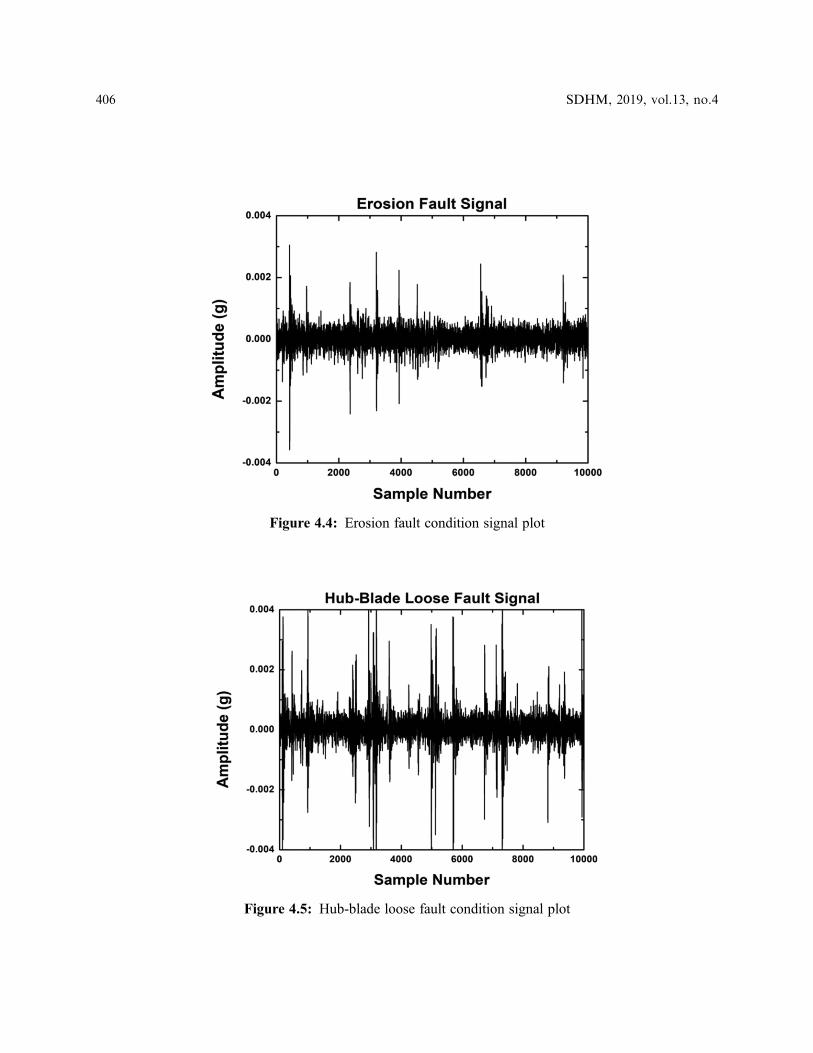
Figure 4.4: Erosion fault condition signal plot

Figure 4.5: Hub-blade loose fault condition signal plot

406 SDHM, 2019, vol.13, no.4

3 Feature Extraction

The vibration signals were obtained for good and other faulty conditions of the blades. If the timedomain sampled signals are given directly as inputs to a classifier, then the number of samples should beconstant. The number of samples obtained is the function of rotational speed. Hence, it cannot be useddirectly as it functions as the input to the classifier. Hence, a few features must be extracted before theacquired vibration signals, the required features were taken and those features are denoted as histogramfeatures. Here, two main factors are to be taken care of while selecting the bins they are, bin width andbin range. The range of bin must be the lowest of minimum amplitude (−0.017988) to the highest ofmaximum amplitude (0.024833) of all the six classes (good, bend, crack, erosion, loose and PAT). Thenumber of bins for the fault diagnosis of the wind turbine blade has been attained by carrying out asequence of trials using a J48 algorithm with a different number of bins. Initially, the range of each bin isseparated into two equivalent portions. That is to say, the number of bins utilized is two. The twohistogram features, to be specific, X1 and X2 were extracted and the corresponding classification accuracywas computed using the J48 decision tree algorithm. The approach and methodology of performing thesame using the J48 decision tree algorithm are explained in Section 4. The classification accuracies werecomputed with various numbers of bins from 2, 3, 4, 5,…, 100 and the corresponding results are shownin Fig. 5.

From Fig. 5, bin size 77 has been chosen since the highest classification accuracy of 92% was found inbin 77. A set of 77 features namely X1, X2… X77 were extracted from the vibration signals and these aredenoted as histogram features. For further study, rather than utilizing vibration signals directly, thehistogram features extracted from vibration signals are utilized. The procedure of calculating applicableparameters of the signals that represent the information contained in the signal is called feature extraction.Histogram analysis of vibration signals yields distinctive parameters. All the extracted histogram features,X1 to X77 extracted from the vibration signals may not contain the needed information for classification.The applicable ones are selected using the J48 decision tree algorithm.

Figure 4.6: Pitch angle twist fault condition signal plot

SDHM, 2019, vol.13, no.4 407

4 J48 Decision Tree Algorithm for Feature Selection

From the extracted features (77), the most contributing features are selected using the feature selectionprocess. For feature selection, the J48 decision tree algorithm is used. The J48 decision tree algorithm isadapted from the C4.5 algorithm in WEKA [13]. It consists of a number of branches, one root, a numberof nodes, and a number of leaves. One branch is a chain of nodes from the root to a leaf, and each nodeinvolves one attribute. The occurrence of an attribute in a tree provides information about the importanceof the associated attribute. A decision tree is a tree-based knowledge representation methodology used torepresent classification rules. J48 decision tree algorithm is a widely used one to construct decision trees[14]. The procedure of forming the decision tree and exploiting the same for feature selection ischaracterized by the following:

1. The set of features available at hand forms the input to the algorithm; the output is the decision tree.

2. The decision tree has leaf nodes, which represent class labels, and other nodes associated with the classesbeing classified.

3. The branches of the tree represent each possible value of the feature node from which they originate.

4. The decision tree can be used to classify feature vectors by starting at the root of the tree and movingthrough it right through to a leaf node, which provides a classification of the instance, is identified.

5. At each decision node in the decision tree, one can select the most useful feature for classification usingappropriate estimation criteria. The criterion used to identify the best feature invokes the concepts ofentropy reduction and information gain.

Information gain measures how well a given attribute separates the training examples according to theirtarget classification. The measure is used to select the candidate among the features at each step whilegrowing the tree. Information gain is the expected reduction in entropy caused by portioning the samplesaccording to this feature. Information gain (S, A) of a feature A relative to a collection of examples S, isdefined as:

Gain S;Að Þ ¼ Entropy Sð Þ �X

v2Value Að Þ �Svj jSj j Entropy Svð Þ (1)

Were Value (A) is the set of all possible values for attribute A, and Sv is the subset of S for which featureA has value v. Note the first term in the equation for gain is just the entropy of the original collection S and the

Figure 5: Classification accuracy vs. bin range

408 SDHM, 2019, vol.13, no.4

second term is the expected value of the entropy after S is partitioned using feature A. The expected entropydescribed by the second term is simply the sum of the entropies of each subset Sv, weighted by the fraction ofsamples |Sv|/|S| that belong to Sv. Gain (S, A) is the expected reduction in entropy caused by knowing thevalue of feature A. Entropy is a measure of homogeneity of the set of examples and it is given by

Entropy Sð Þ ¼Xc

i�1�Pilog2Pi (2)

where c is the number of classes, Pi is the proportion of S belonging to class ‘i’. The J48 decision treealgorithm has been applied to the problem for the feature selection process. The input to the algorithm isthe set of histogram features described above and the output of the decision tree shown in Fig. 6. Itclearly shows that the top node is the best node for classification. The other features in the nodes of adecision tree are seen in descending order of significance [15]. It is to be mentioned here that onlyfeatures that contribute to the classification appear in the decision tree. The features which have less of adiscriminating capability can be consciously discarded by deciding on the threshold. This concept ismade clear for selecting relevant features. The algorithm identifies the relevant features for the purpose ofclassification from the given training data set, and thus reduces the domain knowledge required to select

Figure 6: J48 Tree classification for feature selection

SDHM, 2019, vol.13, no.4 409

good features for pattern classification problem [16, 17]. Referring to Fig. 6, one can identify the mostdominating features to represent the blade conditions are X33, X34, X35, X32, and X36.

5 Feature Classification

After feature selection, the selected features (X33, X34, X35, X32, and X36) were given as input to thetree classifiers like best-first tree (BF), decision stump (DS), extra tree (ET), functional trees (FT), hoeffdingtree (HT), J48 decision tree (J48), J48 consolidated (J48C), J48 graft (J48G), least absolute deviationregression tree (LAD), logistic model tree (LMT), NB Tree (NBT), random forest (RF), random tree(RT), reduced-error pruning tree (REP) and simple cart classifiers (SCC) [18].

5.1 Best-first Tree (BF)Best-first decision tree learning is one kind of decision tree learning that has almost all properties of

standard decision learning. Trees generated by best-first decision tree learning have all propertiesdescribed in Section 4, however, the only difference is that standard decision tree learning expands nodesin depth-first order, while best-first decision tree learning expands the “best” node first. Standard decisiontree learning and best-first decision tree learning generate the same fully-expanded tree for a given data.However, if the number of expansions is specified in advance, the generated trees are different in most cases.

5.2 Decision Stump (DS)A decision stump is a machine learning model comprising of a one-level decision tree. It is also called as

weak learners or base learners. It is a decision tree with one inner hub (the root) which is instantly associatedwith the terminal hubs (its leaves). A decision stump makes a forecast based on the significance of just adistinct input feature. They are additionally called as 1-rules. If the feature is numerical, the tree may bemore complex. Decision stumps are often used as components in machine learning ensemble methodssuch as bagging and boosting.

5.3 Extra Tree (ET)The extra tree algorithm is an ensemble technique that utilizes randomized decision trees. It varies from

other randomized decision trees. With the least parameter setting, the algorithm would entirely randomizeboth the split and the attribute selected at each decision node, yielding a tree completely independent oftraining data. The extra tree is also called as an extremely randomized tree.

5.4 Functional Trees (FT)The functional tree is the classification tree that could have logistic regression functions at the inner

nodes and/or leaves. The algorithm can deal with binary and multi-class target variables, numeric andnominal attributes and missing values. This algorithm is similar to many others, except in the constructivephase. Here a function is built and mapped to new attributes. There are some aspects of this algorithmthat should be made explicit. In the next step, a model is built using the constructor function. This isdone by using only the examples that fall at this node only. Later, the model is mapped to new attributes.The constructor function should be a classifier or a regressor depending on the type of the problem. Inthe former, the number of new attributes is equal to the number of classes, in the latter the constructorfunction is mapped to one new attribute.

5.5 Hoeffding Tree (HT)A hoeffding tree algorithm (HT) is an incremental, anytime decision tree initiation algorithm that is

proficient in learning from substantial data streams, assuming that the distribution producing samplesdoes not change over time. A novel paradigm of hoeffding trees was presented in 2000, which formsmodels that can be verified corresponding to regular decision trees if the data is static and the total

410 SDHM, 2019, vol.13, no.4

number of samples is sufficiently extensive. Hoeffding trees depend on a direct idea known as the hoeffdingbound. It creates natural logic that, given sufficient independent observations, the real mean of a randomvariable will not change from the predictable mean by more than a definite amount.

5.6 J48 Decision Tree (J48)J48 decision tree algorithm is adapted from the C4.5 algorithm in WEKA. It consists of a number of

branches, one root, a number of nodes, and a number of leaves. One branch is a chain of nodes from theroot to a leaf, and each node involves one attribute. Furthermore, the technical aspects of the J48 decisiontree algorithm are explained in Section 4.

5.7 J48 Consolidated (J48C)J48 Consolidated (J48C) algorithm is also called as consolidated tree construction (CTC) algorithm. It

creates a set of subsamples from a training sample and builds a decision tree from each subsample. Instead ofbuilding each tree independently, the decision on each split is voted on by all trees. All trees comply with themajority vote and make the same split regardless of their individual vote. The process is repeated until thetrees agree to stop growing.

5.8 J48 Graft (J48G)It is an extended version of the J48 decision tree algorithm that considers grafting additional branches

onto the tree in a post-processing phase. The grafting process attempts to achieve some of the power ofensemble methods such as bagged and boosted trees while maintaining a single interpretable structure. Itidentifies regions of the instance space that are either empty or contain only misclassified examples andexplores alternative classifications by considering different tests that could have been selected at nodesabove the leaf containing the region.

5.9 Least Absolute Deviation Regression Tree (LAD)LAD Tree (LAD) or least absolute deviation regression tree is an alternating decision tree algorithm that

can handle multiclass problems based on the LogitBoost algorithm. In LAD Tree, the number of boostingiterations is a parameter that can be tuned to the data at hand and determines the size of the tree constructed.

5.10 Logistic Model Tree (LMT)A logistic model tree essentially comprises a standard decision tree structure with logistic regression

tasks at the leaves. As in normal decision trees, a test on one of the qualities is connected with eachinternal hub. For an identified property with k values, the hub has k child hubs, and illustrations aresorted down one of the k branches relying upon their estimation of the feature. For numeric features, thehub has two child hubs and the test comprises contrasting the characteristic signature to the threshold.Generally, a logistic model tree comprises a tree structure that is comprised of an arrangement of internalor non-terminal hubs N and an arrangement of leaves or terminal hubs T. Let S indicate the entireoccurrence in space, spread over by all characteristics that are available in the information. At that point,the tree structure gives a separate section of S into areas St, and each area is characterized by a leaf in the tree.

S ¼ [t2T St; St \ St0 ¼ [ for t 6¼ t0 (3)

5.11 NB-tree (NBT)NB-Tree (NBT) is a hybrid between decision trees and Naïve Bayes. It creates a tree with leaves that are

Naïve Bayes classifiers for the instances that reach the leaf. When constructing the tree, cross-validation isused to decide whether a node should be split further or a Naïve Bayes model used instead.

SDHM, 2019, vol.13, no.4 411

5.12 Random Forest (RF)Random forest (RF) is an idea of the general system of random decision forests that are a group learning

technique for characterization, regression and other different errands. It works by building a large number ofdecision trees while execution and yields the class (classification) or mean prognosis (regression) of theindividual trees. Random decision forests perfect the decision tree's propensity for overfitting to theirtraining set.

5.13 Random Tree (RT)Random decision tree algorithm (RT) builds numerous decision trees arbitrarily. When building each

tree, the algorithm chooses a leftover feature arbitrarily at each hub development without any good rolecheck such as data gain, Gini index, etc. A definite feature such as gender is considered leftover if thesame definite feature has not been chosen earlier in a particular decision path preliminary from the originof the tree to the present hub. Once a definite feature is selected, it is useless to choose it again on thesame decision path because every sample in a similar path will have an identical value.

5.14 Reduced-error Pruning Tree (REP)REP tree (REP) or reduced-error pruning tree builds a decision or regression tree using information gain

or variance reduction and prunes it using reduced-error pruning. For optimized speed, it only sorts values fornumeric attributes. It deals with missing values by splitting instances into pieces, as C4.5 does. One can setthe minimum number of instances per leaf, maximum tree depth (useful when boosting trees), the minimumproportion of training set variance for a split (numeric classes only), and a number of folds for pruning.

5.15 Simple Cart Classifiers (SCC)Simple cart classifier (SCC) is a decision tree learner for classification that employs the minimal cost-

complexity pruning strategy. Though named after the CART (classification and regression tree) learner thatpioneered this strategy, however, the similarity ends here where it provides none of CART’s other features.One can set the minimum number of instances per leaf, the percentage of training data used to construct thetree, and the number of cross-validation folds used in the pruning procedure.

6 Results and Discussion

The vibration signals were noted for good condition and other fault conditions of the blade using a dataacquisition system. Totally 600 samples were collected; out of which, 100 samples were from a goodcondition blade. For different faults such as blade bend, erosion, blade crack, hub-blade loose connection,pitch angle twist, 100 samples from each condition were noted. J48 decision tree algorithm was used toselect the best-contributing features from histogram features. From bin 77, X33, X34, X35, X36, and X32were chosen as the best contributing features [19]. From Fig. 6, the selected features were given as theinput to tree classifiers like a best-first tree (BF), decision stump (DS), extra tree (ET), functional trees(FT), hoeffding tree (HT), J48 decision tree (J48), J48 consolidated (J48C), J48 graft (J48G), leastabsolute deviation regression tree (LAD), logistic model tree (LMT), NB Tree (NBT), random forest(RF), random tree (RT), reduced-error pruning tree (REP) and simple cart classifiers (SCC). Theclassification accuracy of different classifiers with their computational time was presented in Tab. 2. Theobjective of the study is to find, the better the classifier. Amongst the considered classifiers, one canclearly note (from Tab. 2), LMT classifier performs better, compared to other classifiers. This decisionwas made based on high classification accuracy (94.33%) with low computational time (0.27 s). Theconfusion matrix of the LMT is shown in Tab. 3. In the confusion matrix, the diagonal elements representthe correctly classified instances and the others are misclassified instances. The first row of the confusionmatrix, Tab. 3, represents good condition. The first element (the location (1, 1)) represents the number ofcorrectly classified instances belonging to the same [20]. The second element (the location (1, 2))

412 SDHM, 2019, vol.13, no.4

represents the number of good instances that were incorrectly classified as bend fault condition (bend). Thethird element (the location (1, 3)) represents the number of good instances that were incorrectly classified ascrack fault condition (crack). The fourth element (the location (1, 4)) represents the number of good instancesthat were incorrectly classified as erosion fault condition (erosion). The fifth element (the location (1, 5))represents the number of good instances that were incorrectly classified as hub-blade loose fault condition(loose). The sixth element (the location (1, 6)) represents the number of good instances that wereincorrectly classified as pitch angle twist fault conditions (pitch twist). Similarly, the second rowrepresents the second condition i.e., bend fault condition. The third row represents the data points for thethird condition, i.e., crack fault condition. The fourth row represents the data points for the fourthcondition, i.e., erosion fault condition. The fifth row represents the data points for the fifth condition, i.e.,

Table 2: Classification accuracy of the classifiers

S.No Classifiers Classification Accuracy (%) Time (s)

1. BF 92.00 0.75

2. DS 33.33 0.02

3. ET 84.17 0.04

4. FT 92.83 0.72

5. HT 90.83 0.26

6. J48 89.83 0.04

7. J48C 89.17 0.02

8. J48G 89.67 0.07

9. LAD 90.17 0.48

10. LMT 94.33 0.27

11. NBT 89.67 0.75

12. RF 93.00 0.48

13. RT 88.33 0.02

14. REP 90.33 0.02

15. SCC 91.00 0.52

Table 3: Confusion matrix for LMT

Blade conditions Good Bend Crack Erosion Loose PAT

Good 96 0 0 0 4 0

Bend 0 100 0 0 0 0

Crack 1 0 89 1 4 5

Erosion 0 0 3 95 0 2

Loose 4 0 2 0 94 0

PAT 0 0 4 4 0 92

SDHM, 2019, vol.13, no.4 413

hub-blade loose fault condition. The sixth row represents the data points for the sixth condition, i.e., pitchangle twist fault condition [21].

From the confusion matrix (Tab. 3), Out of 600 samples, 566 samples are correctly classified (94.33%)and the remaining 34 are misclassified (5.67%). These 34 misclassification instances occurred because thesehave a similar vibration pattern of the other fault condition. For example, for a crack fault condition, due tohigh wind velocity, the firmness of the blade fails and the vibration pattern of the crack signals may resembleother faults (erosion, loose and PAT) conditions. Because of this, the classifier fails to differentiate among thefaults; hence, more misclassification could have happened. From LMT, the kappa statistics were found to be0.932. It is used to measure the arrangement of likelihood with the true class. The mean absolute error wasfound to be 0.032. It is a measure used to measure how close forecasts or predictions are the ultimate results.The root means a square error was found to be 0.1187. It is a quadratic scoring rule which processes theaverage size of the error. The time taken to build the model is about 0.27 s; hence, this can be used inreal-time for the fault detection on the wind turbine blade. The detailed class-wise accuracy is shown inTab. 4. The class-wise accuracy is expressed in terms of the true positive rate (TP), false positive rate(FP), precision, recall, and F-Measure [22].

TP is used to predict the ratio of positives which are correctly classified as faults. FP is commonlydescribed as a false alarm in which the result that shows a given fault condition has been achieved whenit really has not been achieved [23]. The true positive (TP) rate should be close to 1 and the false positive(FP) rate should be close to 0 to propose the classifier is a better classifier for the problem classification.In LMT, it shows that the TP near to 1 and FP close to 0, hence one can conclude that the classifier builtfor the specific problem is effective for the fault diagnosis problem. Precision is the probability ofretrieved instances that are relevant to the class. That is, it is the ratio of true positive (TP) to theretrieved instances (TP + FP). It is stated as TP/(TP + FP). For example, from Tab. 3, for bend condition,the precision value is calculated as [1.0/(1.0 + 0) = 1.000]. Precision is also called the positive predictivevalue and can be defined as a measure of exactness or quality. The recall is information retrieval whichshows the probability of the faults that are relevant to the classification that is successfully retrieved [24].That is the ratio of true positive (TP) to the overall instances (TP + FN). False-negative (FN) isconsidered as a type 2 error in which the instances indicate the misclassification but it is actuallycorrectly classified. It is stated as TP/(TP + FN). For example, from Tab. 3, for crack condition, the recallis calculated as [0.89/(0.89 + 0.11) = 0.890]. Here 0.11 represents the misclassification (11 instances) incrack fault condition from 100 samples (crack condition alone) [25]. A recall is also called as themeasure of completeness or quantity. F-measure is defined as the harmonic mean of both recall andprecision. That is, this measure is approximately the average of the two (recall and precision) when they

Table 4: Class-wise accuracy of the logistic model tree

Class TP Rate FP Rate Precision Recall F-Measure

Good 0.960 0.010 0.950 0.960 0.955

Bend 1.000 0.000 1.000 1.000 1.000

Crack 0.890 0.018 0.908 0.890 0.899

Erosion 0.950 0.010 0.950 0.950 0.950

Loose 0.940 0.016 0.922 0.940 0.931

PAT 0.920 0.014 0.929 0.920 0.925

414 SDHM, 2019, vol.13, no.4

are close, and is more generally the square of the geometric mean divided by the arithmetic mean. Thef-measure is expressed as 2 * (Recall * Precision)/(Recall + Precision). For example, from Tab. 3, forcrack condition, the f-measure is calculated as [2 * {(0.89 * 0.89)/(0.89 + 0.89)} = 0.890]. The classifiererror chart is shown in Fig. 7. Here the squared dots represent the misclassification and the ‘x’ denotesthe correct classification.

7 Conclusions

The wind turbine is an important structure in extracting wind energy from the accessible wind. Thispaper displays an algorithm based classification of vibration signals for the evaluation of the wind turbineblade conditions. From the acquired vibration data, fifteen models were developed using data modellingtechniques. The models were tested with 10-fold cross-validation. All the classifiers were compared withrespect to their types and maximum correctly classified instances. The maximum classification accuracywas found to be 94.33% for the logistic model tree (LMT). The error rate is relatively less and LMT maybe considered for the blade fault diagnosis. Hence, the logistic model tree (LMT) can be practically usedfor the condition monitoring of wind turbine blades to reduce the downtime and to maximize the usage ofwind energy. The methodology and algorithm suggested in this paper can be potentially used for anykind of wind turbine blade to diagnose the blade fault with minimal modification.

References1. Ciang, C. C., Lee, J. R., Bang, H. J. (2008). Structural health monitoring for a wind turbine system: a review of damage

detection methods. Measurement Science and Technology, 19(12), 1–20. DOI 10.1088/0957-0233/19/12/122001.

2. Ziegler, L., Gonzalez, E., Rubert, T., Smolka, U., Melero, J. J. (2018). Lifetime extension of onshore wind turbines:a review covering Germany, Spain, Denmark, and the UK. Renewable and Sustainable Energy Reviews, 82,1261–1271. DOI 10.1016/j.rser.2017.09.100.

3. Joshuva, A., Sugumaran, V. (2019). Improvement in wind energy production through condition monitoring ofwind turbine blades using vibration signatures and ARMA features: a data-driven approach. Progress inIndustrial Ecology, 13(3), 207–231.

Figure 7: Classifier errors (classification vs misclassification)

SDHM, 2019, vol.13, no.4 415

4. Li, D., Ho, S. C., Song, G., Ren, L., Li, H. (2015). A review of damage detection methods for wind turbine blades.Smart Materials and Structures, 24(3), 1–24.

5. Kusiak, A., Zheng, H., Song, Z. (2009). Models for monitoring wind farm power. Renewable Energy, 34(3),583–590. DOI 10.1016/j.renene.2008.05.032.

6. Kusiak, A., Zhang, Z. (2015). Adaptive control of a wind turbine with data mining and swarm intelligence. IEEETransactions on Sustainable Energy, 2(1), 28–36.

7. Godwin, J. L.,Matthews, P. (2013). Classification and detection of wind turbine pitch faults through SCADAdata analysis.International Journal of Prognostics and Health Management (IJPHM) Special Issue on Wind Turbine PHM,4(Special Issue 2), 1–11.

8. Pratumnopharat, P., Leung, P. S., Court, R. S. (2014). Wavelet transform-based stress-time history editing ofhorizontal axis wind turbine blades. Renewable Energy, 63, 558–575. DOI 10.1016/j.renene.2013.10.017.

9. Benim, A. C., Diederich, M., Nikbay, M. (2015). Optimization of airfoil profiles for small wind turbines. In: 8thICCHMT, Istanbul.

10. Vučina, D., Marinić-Kragić, I., Milas, Z. (2016). Numerical models for robust shape optimization of wind turbineblades. Renewable Energy, 87, 849–862. DOI 10.1016/j.renene.2015.10.040.

11. Liu, W. (2016). Design and kinetic analysis of wind turbine blade-hub-tower coupled system. Renewable Energy,94, 547–557. DOI 10.1016/j.renene.2016.03.068.

12. Ou, Y., Chatzi, E. N., Dertimanis, V. K., Spiridonakos, M. D. (2017). Vibration-based experimental damage detectionof a small-scale wind turbine blade. Structural Health Monitoring, 16(1), 79–96. DOI 10.1177/1475921716663876.

13. Quinlan, J. R. (1996). Improved use of continuous attributes in C4.5. Journal of Artificial Intelligence Research, 4,77–90. DOI 10.1613/jair.279.

14. Joshuva, A., Sugumaran, V. (2017). A data driven approach for condition monitoring of wind turbine blade usingvibration signals through best-first tree algorithm and functional trees algorithm: a comparative study. ISATransactions, 67, 160–172. DOI 10.1016/j.isatra.2017.02.002.

15. Indira, V., Vasanthakumari, R., Sugumaran, V. (2010). Minimum sample size determination of vibration signals inmachine learning approach to fault diagnosis using power analysis. Expert Systems with Applications, 37(12),8650–8658. DOI 10.1016/j.eswa.2010.06.068.

16. Peck, R., Devore, J. L. (2012). Statistics: the exploration and analysis of data (7th ed.). Boston: Brooks/Cole,Cengage Learning.

17. Joshuva, A., Sugumaran, V. (2019). Crack detection and localization on wind turbine blade using machine learningalgorithms: a data mining approach. Structural Durability & Health Monitoring, 13(2), 181–203. DOI 10.32604/sdhm.2019.00287.

18. Mitchell, T. M. (1997). Machine learning. Burr Ridge: McGraw Hill, 45.

19. Sharma, T. C., Jain, M. (2013). WEKA approach for comparative study of classification algorithm. InternationalJournal of Advanced Research in Computer and Communication Engineering, 2(4), 1925–1931.

20. Joshuva, A., Sugumaran, V. (2019). Selection of a meta classifier-data model for classifying wind turbine bladefault conditions using histogram features and vibration signals: a data-mining study. Progress in IndustrialEcology, 13(3), 232–251. DOI 10.1504/PIE.2019.10022055.

21. Sharma, A. K., Sahni, S. (2011). A comparative study of classification algorithms for spam email data analysis.International Journal on Computer Science and Engineering, 3(5), 1890–1895.

22. Powers, D. M. (2011). Evaluation: from precision, recall and F-measure to ROC, informedness, markedness andcorrelation. International Journal of Machine Learning Technology, 2(1), 37–63.

23. Manju, B. R., Joshuva, A., Sugumaran, V. (2018). A data mining study for condition monitoring on wind turbineblades using hoeffding tree algorithm through statistical and histogram features. International Journal ofMechanical Engineering and Technology, 9(1), 1061–1079.

24. Hall, M., Frank, E., Holmes, G., Pfahringer, B., Reutemann, P. et al. (2009). The WEKA data mining software: anupdate. ACM SIGKDD Explorations Newsletter, 11(1), 10. DOI 10.1145/1656274.1656278.

25. Joshuva, A., Sugumaran, V. (2017). A comparative study of Bayes classifiers for blade fault diagnosis in windturbines through vibration signals. Structural Durability and Health Monitoring, 12(1), 69–90.

416 SDHM, 2019, vol.13, no.4