COMPARATIVE ANALYSIS OF LMS (LEAST MEAN …ibt.edu.pk/qec/jict/10.1/4.pdf · Sir Syed University of...

Journal of Information & Communication TechnologyVol. 10, No. 1, (Spring 2016) 35 - 46

* The material presented by the author does not necessarily portray the viewpoint of the editorsand the management of the Institute of Business & Technology (IBT)

© IBT-JICT is published by the Institute of Business and Technology (IBT). Main Ibrahim Hydri Road, Korangi Creek, Karachi-75190, Pakistan.

COMPARATIVE ANALYSIS OF LMS (LEASTMEAN SQUARE) AND RLS (RECURSIVE LEAST

SQUARE) FOR ESTIMATION OF FIGHTERPLANE’S MATHEMATICAL MODEL

Muhammad Tahir Qadri1

Department of Electronic EngineeringSir Syed University of Engineering & Technology

Rakshan Zulfikar2

Department of Telecommunication EngineeringSir Syed University of Engineering & Technology

Nimrah Ahmed3


Rumaisa Iftikar4


Key Words: System Identification, Least Mean Square (LMS),Recursive Least Square (RLS), Modeling Of Fighter Plane.INSPEC Classification : A9555L, A9630, B5270

ABSTRACTEstimating of complex system in real time environment is necessary fordesigning a precise controller to operate the given system. In this paperwe have compared both Least Mean Square (LMS), and Recursive LeastSquare to identify which one of them gives more approximate estimation.Basically LMS is based on the set of Adaptive filters tends to reduce theerror over time between the actual system response and the desired systemresponse, on the other hand we have RLS that is capable of forgetting theprevious acquired data and focus on recent main stream data. We haveconsidered a model of a fighter plane because of its complex and unpredictedmovements to estimate the model at its follows. Both the algorithms arecomplete and useful, but their usage may vary according to the application.

Ali Akbar Siddiqui5Department of Telecommunication Engineering

Sir Syed University of Engineering & Technology

1 Muhammad Tahir Qadri : [email protected] Rakshan Zulfikar : [email protected] Nimrah Ahmed : [email protected] Rumaisa Iftikar : [email protected] Ali Akbar Siddiqui : [email protected]

1. INTRODUCTION

Aircraft formation is identified to be prone to nonlinear occurrence, particularlynowadays as they are lighter in weight and more flexible (J.P. No¨el ET.AL, 2005).The major setback in the formation of flight control system is the designing of uncertainparametric variation of any aircraft (Eugene A. Morelli, 2006). We have considered themodel of F-16 (Morelli, E.A, 1998), that it is an example of nonlinear model. Our workhere presents a viability study of technique for identification and estimation of uncertainparameters of fighter aircraft. The major aim of this research is to investigate thepossibility of a method through which coefficient identification and estimation becomesfeasible.

Jet consists of various model parameters as well as one or multiple inputs (Morelli,E.A, 1998). In most cases, the target is to determine a structure of model that is notonly compact, but still has ample complexity to determine all the nonlinearities (Klein,V. and Morelli, E, 2006). Previously, a method was developed to estimate input andoutput flight data through frequency response estimation which was not only timeconsuming but costly too (Tischler, M. and Remple, R., 2011). Another technique hasbeen developed to estimate the aerodynamic parameters without the involvement ofairflow angles, while this method offered reduction of cost in testing of flight, insinuationsfor safety of aircraft were noted (Eugene A. Morelli, 2012). One approach observedfor parameter estimation is nonlinear sliding surface control which provided fairlyaccurate estimation but was unable to guarantee stability or convergence (Gurbacki,Phillip, 2010).

An additional process to estimate the parameters is to consider that the dynamicmodel include the linear structure with respect to time variant parameters to explainthe changes occurring in flight condition; however the major problem afflicted here inparameter estimation is by noise. Perfectly estimating the aerodynamic parameters isvital for control systems that require the estimated parameters as inputs.

Our paper offers calculation of aerodynamic parameters while proving to be stable,convergent as well as robust. The parameter estimator explored here is Least MeanSquare (LMS) and Recursive Least square (RLS). LMS having applications fromeconomy growth to aerodynamics is considered to be extremely popular for adaptivesystem identification (Gurbacki, Phillip, 2010). LMS include an iterative process thatformulates consecutive modification to main vector in the direction of the negative ofthe gradient vector that ultimately escort to the minimum mean square error. Thisestimator has proven to be superior adaptive estimator.

The main focus of our research is the three dimensions, in which the flight freelyrotates, i.e. pitch (lateral), yaw (normal) and roll (longitudinal). The mentioned axesprogress with the aircraft while rotating relative to the Earth (Gui and Adachi, 2013).The rotations are created due movement of control surfaces that offers variation indistribution of the

36Vol. 10, No. 1, (Spring 2016)

Muhammad Tahir Qadri, Rakshan Zulfikar, Nimrah Ahmed, Rumaisa Iftikar, Ali Akbar Siddiqui

overall aerodynamic force with respect to the centre of gravity of the aircraft. Theseaxes are considered to be symmetrical geometrically in spite of mass distribution ofjet (Eleftherios Giovanis, 2008).

In this paper section II describes the fighter plane dynamics which includes fighterplane dynamics, coordinate system and equation of motion. Section III is our estimationalgorithm; least mean Square. Discussions and results are covered in section IV.

2. LITERATURE REVIEW

2.1 Fighter Plane Dynamics

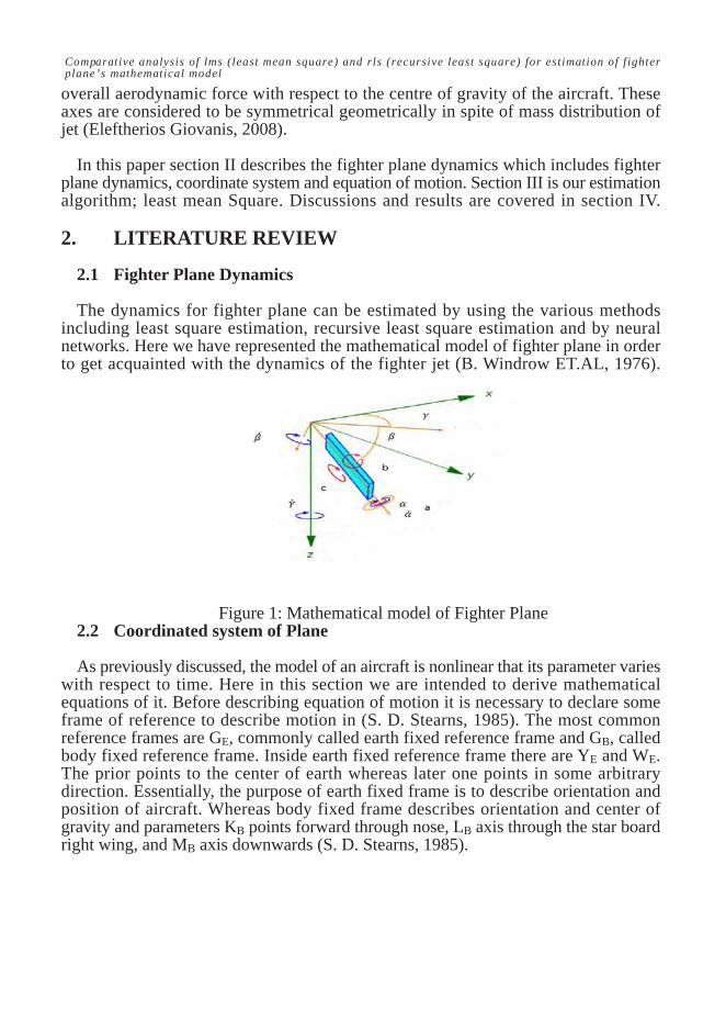
The dynamics for fighter plane can be estimated by using the various methodsincluding least square estimation, recursive least square estimation and by neuralnetworks. Here we have represented the mathematical model of fighter plane in orderto get acquainted with the dynamics of the fighter jet (B. Windrow ET.AL, 1976).

As previously discussed, the model of an aircraft is nonlinear that its parameter varieswith respect to time. Here in this section we are intended to derive mathematicalequations of it. Before describing equation of motion it is necessary to declare someframe of reference to describe motion in (S. D. Stearns, 1985). The most commonreference frames are GE, commonly called earth fixed reference frame and GB, calledbody fixed reference frame. Inside earth fixed reference frame there are YE and WE.The prior points to the center of earth whereas later one points in some arbitrarydirection. Essentially, the purpose of earth fixed frame is to describe orientation andposition of aircraft. Whereas body fixed frame describes orientation and center ofgravity and parameters KB points forward through nose, LB axis through the star boardright wing, and MB axis downwards (S. D. Stearns, 1985).

Comparative analysis of lms (least mean square) and rls (recursive least square) for estimation of f ighterplane’s mathematical model

Figure 1: Mathematical model of Fighter Plane2.2 Coordinated system of Plane

overall aerodynamic force with respect to the centre of gravity of the aircraft. Theseaxes are considered to be symmetrical geometrically in spite of mass distribution ofjet (Eleftherios Giovanis, 2008).

In this paper section II describes the fighter plane dynamics which includes fighterplane dynamics, coordinate system and equation of motion. Section III is our estimationalgorithm; least mean Square. Discussions and results are covered in section IV.

2. LITERATURE REVIEW

2.1 Fighter Plane Dynamics

The dynamics for fighter plane can be estimated by using the various methodsincluding least square estimation, recursive least square estimation and by neuralnetworks. Here we have represented the mathematical model of fighter plane in orderto get acquainted with the dynamics of the fighter jet (B. Windrow ET.AL, 1976).

Figure 1: Mathematical model of Fighter Plane2.2 Coordinated system of Plane

As previously discussed, the model of an aircraft is nonlinear that its parameter varieswith respect to time. Here in this section we are intended to derive mathematicalequations of it. Before describing equation of motion it is necessary to declare someframe of reference to describe motion in (S. D. Stearns, 1985). The most commonreference frames are GE, commonly called earth fixed reference frame and GB, calledbody fixed reference frame. Inside earth fixed reference frame there are YE and WE.The prior points to the center of earth whereas later one points in some arbitrarydirection. Essentially, the purpose of earth fixed frame is to describe orientation andposition of aircraft. Whereas body fixed frame describes orientation and center ofgravity and parameters KB points forward through nose, LB axis through the star boardright wing, and MB axis downwards (S. D. Stearns, 1985).

37 Journal of Information & Communication Technology


38Vol. 10, No. 1, (Spring 2016)

2.3 Description of variables

Before pursuing to the equations of motions, some preliminary assumptions havebeen taken into account. A valid assumption for fighter plane is that the air craft is rigidbody which reflects that on any two points or within the frame remains fixed withrespect to each other. Also, it is tacit for control design of aircraft that earth is flat, nonerotating regarded as an inertial reference but not valid for inertial guidance system. Themass is considered constant during which the motion of aircraft is under considerationand fuel consumption is neglected during this time. It is necessary to apply Newton’smotions law on this assumption. Similarly, the symmetry in mass distribution of aircraftis relative to KBOMB, which means that product of inertia Vxy and Vyz equals to zero(S. Haykin, 2002).

As a result of mentioned assumptions the aircraft’s motion has 6 degree of freedom(DOF) rotation and translation in dimensions; position, orientation, velocity and angularvelocity over time describe aircraft dynamics (M. G. Bellanger, 2011).

BE=(AE,BE,CE )T position vector expressed in an earth fixed co-ordinate system.

δ=(α,β,γ)T Orientation vector where as α = rollangle,β = pitch angle and γ=yaw angle.

w = (a,b,c)T Angular velocity where a = roll angular velocity, b=pitch angular velocityand c=yaw angular velocity.

2.4.1 Euler angle rates

Euler angle rates and body axis rates, orthogonal body axis angular rate vector:

Non-orthogonal vector of Euler’s angle:

Euler angle rate vector:

2.4 Equations Of Motions



Relationship between Euler’s angle Rates and body axis Rates:

2.4.2 Rigid Body Equations of Motion

Translational position:

Angular position:

Whereas inertia matrix of the aircraft is given by

Where,

Aerodynamic and thrust moment,

Rate of change of Angular velocity,

a’ = (QzzG+QxzI-{Qxz(Qyy-Qxx-Qzz)a+[Qxz+Qzz(Qzz-Qyy)c}b)/(QxxQzz-Qxz) (10)

b’= 1/Qyy[H-(Qxx-Qzz)ac-Qxz(p2-r2)] (11)

c’=[Qxz+ QxxN-{Qxz(Qyy-Qxx-Qzz)r+[Qxz2+Qxx(Qxx-Qyy)]a}b)/QxxQzz-Qxz2] (12)


3. ESTIMATION ALGORITHM

Good estimates are extremely important for control schemes. For stochastic systems,parameters having uncertainties and time delays, robust control and filtering has gainedsignificant amount of research work. With fast developments of control systems,beneficial efforts for flexible and effective models have been made. A motivation todevelop adaptive control aroused to handle parametric uncertainties greater than thosewhich can be handled by robust control. Over the last few decades, adaptive methodsfor controlling and identification of dynamical linear time invariant systems have beendeveloped, utilizing unknown parameters.

Various researches and literature is present in this field, describing methods that arerobust as well as stable with small uncertainty in plant parameters or the parametricchanges occur slowly with respect to time. However, in certain fields like neuroscience,economics, biology and medicines, etc there is a rapid change in parameters with time.Therefore, the solutions presented in are inadequate to cope with the variations. Thereis a need of new methods for identifying and controlling unknown systems quickly.A realistic control design must be robust, stable, as well as maintains performance withrespect to uncertainties in plant such as bounded dynamics. Unknown values of thephysical variables and big parametric uncertainties present in plant dynamics shouldbe handled by the controlled design. It is observed that in past few years, large parametricerrors may cause oscillatory and transient response of adaptive system and constantefforts are made to improve.

3.1 Least Mean square (LMS)

Least mean squares (LMS) algorithms are a set of adaptive filter used to imitate apreferred filter by finding the filter coefficients that relate to producing the least meansquares of the error signal that is, the difference between the desired and the actualsignal.

The LMS is an exploration algorithm in which a generalization of the gradient vectorcalculation is made promising by suitably adjusts the purposed function [16]. The LMSalgorithm is extensively used in a variety of application of adaptive filtering due to itscomputational ease [17] [18] [19].The LMS algorithm is by far the mainly used algorithmin adaptive filtering for numerous bases like stability when executed with set precisionarithmetic, slow convergence and strong performance against unlike signal environment.

The least mean squares (LMS) algorithms fine-tune the filter coefficients to lessenthe cost function. As contrast to recursive least squares (RLS) algorithms, the LMSalgorithms do not engage with any matrix operations. Therefore, the LMS algorithmsrequire less computational resources and memory than the RLS algorithms andimplementation is also less complex than RLS.

40Vol. 10, No. 1, (Spring 2016)


For the expectation process, an increasingly accepted method is least square estimationfor planting bounded rationality in a model. The least square method entails to theagents included in the model to utilize data generated through the model so that leastsquare foretells prospect variables and that the forecasted variables are revised eachtime a new data update is available. In every period of the model, all agents utilizesame forecasts of least squares’ expected values in the system model. The forecastedvariables are inside the model of the system and outcome in the current value in thesystem model, demonstrating consistency with the projections. The provided data, fromthe period, presents a new set of data points which is further used for the updating ofthe least square coefficients in the forecasting equations. The next period use the newcoefficients into the model. The disadvantage of least square is the sensitivity it offersto outliers. A couple of unusual point’s presence may cause tremendous skew in thefinal result.

3.2 Recursive Least Square (RLS)

For system identification of adaptive control and filtering, recursive least squaremethod is an attractive alternative for the reduction of the computational load whichis part and parcel of least square method. Recursive least square is a confined form ofKalman filter.

For accurate description of behavior of systems least square method was introduced.In least square estimation, a linear model of unknown parameter is selected that thesum of the square of the errors between observed values and computed value is lowest.If parametric values of system changes rapidly, cyclic resetting of the estimation methodcan potentially confine the latest values of the parameter. A special heuristic but efficientapproach is used for the parameters which varies continuously but at a snail's pace.

The concept of forgetting is that in which preceding data is step by step discardedin favor of further current information. In least square methodology, forgetting can beexamined as gaining less consideration to previous data and more to recent data. Theclassical recursive least square was not capable of tracking parametric changes as itscovariance vanishes to zero with respect to time. Recursive least square with forgettinghas been widely used in tracking and estimation of parameters which are varied withtime in several fields of engineering. With the poor excitation of system, this schemecan show the way to the covariance wind up problem. Many techniques have beensuggested to tackle covariance windup issues. Several researchers suggested bindingthe expansion of covariance matrix by introducing an upper bound. Time varyingforgetting factor is a renowned scheme used by Fortes cue.

RLS for the q-th order can be expressed as,

Q = Order of the filter.



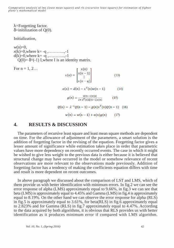
λ=Forgetting factor.δ=initilization of Q(0).

Initialization,

w(n)=0,x(k)=0,where k= -q ,………...,-1d(k)=0,where k= -q ,………...,-1

Q(0)= δ^(-1) I,where I is an identity matrix.

For n = 1, 2…

4. RESULTS & DISCUSSION

The parameters of recursive least square and least mean square methods are dependenton time. For the allowance of adjustment of the parameters, a smart solution is theaddition of forgetting factor in the revising of the equation. Forgetting factor gives alesser amount of significance while estimation takes place in order that parametricvalues have more dependency on recently occurred events. The case in which it mightbe wished to give less weight to the previous data is either because it is believed thatstructural change may have occurred in the model or somehow relevance of recentobservations are more relevant to the observations made previously. Addition offorgetting factor has a tendency of making the coefficients equation differs with timeand result is more dependent on recent outcomes.

In above paragraph we discussed about the comparison of LST and LMS, which ofthem provide us with better identification with minimum errors. In fig.2 we can see theerror response of alpha (LMS) approximately equal to 9.66%, in fig.3 we can see thatbeta (LMS) is approximately equal to 4.45% and Gamma (LMS) in fig.4 is approximatelyequal to 8.19%. On the other hand we can observe the error response for alpha (RLS)in fig.5 is approximately equal to 3.61%, for beta(RLS) in fig.6 approximately equalto 2.823% and for Gamma (RLS) in fig.7 approximately equal to 4.47%. Accordingto the data acquired by both algorithms, it is obvious that RLS provides us with betteridentification as it produces minimum error if compared with LMS algorithm.

42Vol. 10, No. 1, (Spring 2016)


Figure 2: Approximate and error response for LMS (Alpha)

Figure 3: Approximate and error response for LMS (Beta)

Figure 4: Approximate and error response for LMS (Gamma)



Figure 5: Approximate and error response for RLS (Alpha)

Figure 6: Approximate and error response for RLS (Beta)

Figure 7: Approximate and error response for RLS (Gamma)

44Vol. 10, No. 1, (Spring 2016)

CONCLUSION

After analyzing the results of both the algorithm, we can conclude that RecursiveLeast square (RLS) provides us with better estimation of an unknown model as comparedto Least mean square (LMS) algorithm. We have analyzed the results of a fighter planemathematical model with respect to RLS and LMS to identify which one of themprovides us with minimum error. So in the end, error generated by RLS in determiningthe exact model was less than LMS clearly showing that it provides us with betterestimation than LMS for given task.

ACKNOWLEDGMENT

The authors would like to thank Sirsyed University, Karachi for their support in thecompletion of this research work.

REFERENCES

J.P. No¨el, L. Renson, G. Kerschen, B. Peeters, S. Manzato, J. Debille. January (2005)Nonlinear Dynamic Analysis Of An F-16 Aircraft Using GvtData QianWangandRobert F. Stengel, “Robust Nonlinear Flight Control of a High-PerformanceAircraft” IEEE Transactions On Control Systems Technology, Vol. 13, No.1,pp.254-256.

Eugene A. Morelli. August (2006) Practical Aspects of the Equation-Error Method forAircraft Parameter Estimation, Atmospheric Flight Mechanics Conference,Keystone, CO, pp.58.

Morelli, E.A. May (1998) Advances in Experiment Design for High PerformanceAircraft, AGARD System Identification Specialists Meeting, Madrid, Spain,pp.65-68.

Morelli, E.A. (1998) Global Nonlinear Parametric Modeling with Application to F-16Aerodynamics, ACC paper WP04-2, Paper ID i-98010-2, American ControlConference, Philadelphia, Pennsylvania, pp.128.

Klein, V. and Morelli, E. (2006) Aircraft System Identification: Theory and Practice,AIAA Education Series, AIAA, Mexico, pp.196-201.

Eugene A. Morelli. July-August (2012) Real-Time Aerodynamic Parameter Estimationwithout Air Flow Angle Measurements, Journal of Aircraft, Vol. 49, No. 4, pp.1064-1074.

Gurbacki, Phillip.(2010) Feasibility study of a novel method for real-time aerodynamiccoefficient, Estimation Rochester Institute of Technology, Springer, pp.2019-2023.


Morelli, E.A. September-October (2000) Real-Time Parameter Estimation in theFrequency Domain, Journal of Guidance, Control, and Dynamics, Vol. 23,No. 5, pp. 812-818

B Widrow. (1985) SD Stearns, Adaptive Signal Processing, Prentice Hall, New Jersey,pp.135.

Gui and Adachi. (2013) Improved least mean square algorithm with application toadaptive sparse channel estimation, EURASIP Journal on WirelessCommunications and Networking, pp. 2013-2020.

EleftheriosGiovanis.(2008) Applications of Least Mean Square (LMS) AlgorithmRegression in Time-Series Analysis” Munich Personal RePEc Archive, USA,pp.304.

B.Widrow, J. M. McCool, M. G. Larimore, and C. R. Johnson, Jr. August (1976)Stationary and non-stationary learning characteristics of the LMS adaptivefilters,’ Proceedings of the IEEE, vol. 64, pp. 1151-1162.

S. Haykin. (2002) Adaptive Filter Theory, Prentice Hall, Englewood Cliffs, NJ, 4thEdition, Spain, pp.23-28.

M. G. Bellanger .(2001) Adaptive Digital Filters and Signal Analysis, Marcel Dekker,Inc., New York, NY, 2nd edition,pp.1120-1125.

46Vol. 10, No. 1, (Spring 2016)


COMPARATIVE ANALYSIS OF LMS (LEAST MEAN …ibt.edu.pk/qec/jict/10.1/4.pdf · Sir Syed University of...

Documents

Transcript of COMPARATIVE ANALYSIS OF LMS (LEAST MEAN …ibt.edu.pk/qec/jict/10.1/4.pdf · Sir Syed University of...