Compacted Greenspace and Stormwater Hydrology in Burlington, Vermont:

An analysis of 3 remediation treatments for compacted soils and a comparison of stormwater from two small urban catchments.

A Thesis Presented

By

Nathan Arun Toké

To

The Honors Committee of

The University of Vermont

As partial fulfillment of a Bachelor of Science in Geology Through the Department of Geology of

The University of Vermont

May, 2003

Abstract

From May through November, 2002, I monitored experimental test plots to

compare different techniques for remediating compacted soil. I completed three rounds of

testing during which I simulated runoff, measured suspended sediment production, and

collected runoff samples for dissolved elemental analysis. The test plots revealed that

steady-state infiltration rates could be increased by as much as 10 times, from 1.5 cm/h to

15cm/h, by treating compacted soils with aeration, compost, grass seed, and isolation

from further compaction. This method of remediation reduced suspended sediment

production from 34 (g/m2)/ (cm of rainfall) to less than 0.5 (g/m2)/ (cm of rainfall).

Stormwater flow was measured and samples for chemical analysis were collected

from weirs constructed at the outflow of two small drainage basins in Burlington,

Vermont: Perkins Parking lot (4800 m2) and Brookes Avenue (900 m2). Two storm

events were sampled in September, 2002: a 1 hour, 0.81cm, precipitation event on

9/11/02 and a 12 hour, 6.58cm, storm. The Perkins basin has approximately 85%

impermeable cover. The Brookes Avenue basin has approximately 75% impermeable

cover. Storm water discharge responded rapidly to variations in rainfall. Conductivity

showed dilution over time in both basins and during both storm events. Elemental

analysis of Ag, Al, As, Ca, Cd, Cr, Cu, Fe, K, Mg, Na, Ni, P, Pb, Si, Sr, and Zn showed

that at least 8 of the EPA’s priority pollutants are present within runoff from the two

basins. Pb was found in excess, 0.015 to 0.033 ppm, of the EPA’s MCL in the runoff of

both basins during the long-duration storm. The lead MCL was exceeded for 20 and 60

minutes at the Perkins and Brookes basins, respectively. Concentrations of all elements

were highest in the initial samples collected during the storm events. Dissolved element

loading estimates suggest that contaminant sources are different between the two

drainage basins. Higher normalized loadings were seen for the short-duration storm

event. Brookes Avenue had more intense loadings of K, Na, P, Pb, and Zn while Perkins

Parking lot contributed more intense loading of Al, As, Ca, Cr, Cu, Fe, Mg, Ni, Si, and

Sr.

TABLE OF CONTENTS

Chapter Page

List of Tables............................................................................................................................................iii List of Figures .......................................................................................................................................... iv Acknowledgements ................................................................................................................................... v

CHAPTERS

CHAPTER 1 – Introduction........................................................................................................ 1

Literature Review ....................................................................................................... 2 Characterizing the Urban Runoff Problem ................................................................... 2 Water Quality Issues in Burlington, VT ....................................................................... 3 Loss of Greenspace in Burlington, VT......................................................................... 4 Stormwater flow and quality over impervious land...................................................... 6 Compacted soils, traffic, tillage, and compost .............................................................. 9 Research Setting ....................................................................................................... 10 Municipal and Meteorological Setting ....................................................................... 10 Brookes Avenue Drainage Basin................................................................................ 11 Perkins Parking Lot Drainage Basin........................................................................... 12 Campus Remediation Sites ......................................................................................... 14

CHAPTER 2 – Methodology.................................................................................................... 16

Remediation of Compacted Plots on Campus ............................................................ 16 Collection of Burlington Event Sampling Data .......................................................... 18 Drainage Basin Delineation and Land Permeability................................................... 21 ICAP Elemental Analysis ........................................................................................... 22 Data Analysis.............................................................................................................. 22

CHAPTER 3 – Data.................................................................................................................. 24

Vegetative recovery over the remediation test plots................................................... 24 Infiltration rates from the remediation test plots......................................................... 25 Suspended Sediment within the runoff from the remediation plots............................ 25 Water chemistry of the remediation test plots runoff ................................................. 26 Stormwater Runoff Events ......................................................................................... 27 Stormwater Flow, pH and Conductivity ..................................................................... 27 Stormwater Chemistry ................................................................................................ 29

CHAPTER 4 – Discussion........................................................................................................ 32

Changes in steady state infiltration rates with remediation treatment ........................ 32 Changes in normalized suspended sediment loading with remediation treatment...... 33

i

Changes in contaminant concentrations from the remediation test plots.................... 34 Stormwater flow, pH, and conductivity analysis ........................................................ 35 Stormwater Chemistry ................................................................................................ 37

CHAPTER 5 – Conclusions...................................................................................................... 39

REFERENCES........................................................................................................................................ 41

APPENDICIES

Appendix A – Flow data

Appendix B – Chemistry data

Appendix C – Flow and Chemistry Figures

Appendix D – Minitab outputs

Appendix E – Rational runoff estimation

ii

List of Tables:

Chapter 1

Table 1.1 – Brookes Avenue Drainage Basin Description

Table 1.2 – Perkins Drainage Basin Description

Chapter 3

Table 3.1 – Infiltration Rate Statistics Matrix

Table 3.2 – Comparison of Suspended Sediment Loads

Table 3.3 – Suspended Sediment Statistics Matrix

Table 3.4 – Priority Pollutant Test Plot Concentrations

Table 3.5 – Other Element Plot Concentrations

Table 3.6 – Rainfall vs. Runoff Comparison, Perkins 9/11/02

Table 3.7 – Rainfall vs. Runoff Comparison, Brookes 9/11/02

Table 3.8 – Rainfall vs. Runoff Comparison, Perkins 9/27/02

Table 3.9 – Rainfall vs. Runoff Comparison, Brookes 9/27/02

Table 3.10 – Summary Table Perkins 9/11/02

Table 3.11 – Summary Table Brookes 9/11/02

Table 3.12 – Summary Table Perkins 9/27/02

Table 3.13 – Summary Table Brookes 9/27/02

Table 3.14 – Rational Runoff Method Corrected and Normalized Loading Comparison

Chapter 4

Table 4.1 – Stormwater Sources for Contaminants

iii

List of Figures:

Chapter 1

Figure 1.1 – Location map

Figure 1.2 – Brookes Avenue land cover and drainage basin delineation

Figure 1.3 – Perkins Parking lot land cover and drainage basin delineation

Figure 1.4 – Compaction at Cook

Chapter 2

Figure 2.1 – Cook remediated

Figure 2.2 – Cook remediation methods

Figure 2.3 – Infiltration tests

Figure 2.4 – Perkins weir design

Figure 2.5 – Remediation treatment statistical flow chart

Chapter 3

Figure 3.1 – Cook plot comparison of normalized suspended sediment

Figure 3.2 – Changes in sodium concentration by test plot

Figure 3.3 – Discharge and precipitation, Brookes Avenue 9/11/02

Figure 3.4 – Discharge and precipitation, Perkins Lot, 9/27/02

Figure 3.5 – Discharge, pH and conductivity, Brookes Avenue 9/11/02

Figure 3.6 – Calcium concentration and discharge with runoff discharge, Perkins 9/11/02

iv

Acknowledgements

I would like to acknowledge the David Hawley fund, the Lake Champlain Basin

Commission, and the Lintilhac Foundation for their support of this research. This

research is in association with the Urban Hydrology Research Group through the

Department of Geology at the University of Vermont. The research group is headed by

Professor Paul Bierman; we are interested in the problem of greenspace loss and its

effects upon Lake Champlain and the city of Burlington.

I received much help in the field from members of this research group including

Paul Bierman, Lyman Persico, Jackie Hickerson, and Megan Mcgee. I would like to

thank Beverley Wemple and Breck Bowdin for their insights and suggestions as members

of my college honors committee. I must also recognize the John Dewey Honors Program

and Professor Taylor for the support I received throughout my 4 years at UVM. Most

importantly, I thank my thesis advisor, Paul Bierman, for his tremendous dedication to

helping me work through the thesis process which included assisting me in sample

collection, weir construction at all hours of the night, and many weeks of intense editing.

I would also like to thank those closest to me for their support during my college

career and throughout the thesis process including my parents Carolyn and Ray Miller

and Arun Toké and family, Michael and Lois Lynch, Eleanor and Norman Garland,

Prakash Toké and family, Paul Garland and family, Shashi Das and family, and my close

friends including Christyanne, Alysa, Jeff, Jason, Matt, Pete, Rainer, Shaun, my younger

brother Shyam, as well as all other family, friends, and teachers that have helped me

along the way.

v

Chapter 1 Introduction

Some neighborhoods in Burlington, Vermont have lost a significant amount of

greenspace within the past few decades, up to 50% between 1978 and 1999 (Nichols et.

al, in press). This loss of green space is a result of landlords and tenants converting lawns

into informal and formal parking areas. Replacement of permeable greenspace (lawns) by

informal and formal parking areas (pavement and compacted soil) has important effects

on the urban hydrologic cycle and in many cases violates Burlington zoning laws

(geology.uvm.edu/morphwww/urbanhydro/paulm/urbanhydrohomepage.html).

Impermeable land cover significantly influences the urban hydrologic cycle,

causing increased storm peak discharges and contaminant transport capacities (Dennison,

1996); however, water chemistry and flow characteristics from areas where urban runoff

originates are not well quantified. My study attempts to understand, hydrologically, how

small urban catchments respond physically and chemically during storm events. I also

use experimental plot data to address ways to remediate greenspace damaged by

compaction and thus improve stormwater quality and decrease stormwater runoff.

My research consists of two main components. One component involved the direct

measurement of stormwater discharge and the collection of water chemistry samples

from two small urban catchments in Burlington, Vermont, Brookes Avenue (920 m2) and

Perkins Parking lot (4820 m2). These sites were sampled during two storm events in

September 2002. My research reveals characteristics and differences in stormwater runoff

volume and dissolved chemical loading between the two drainage basins and two

sampled storm events. The second component of my research examined changes in water

1

quality and steady state infiltration rates over three rounds of simulated rainfall testing on

eleven remediation test sites on the University of Vermont campus. These test sites

included three variations in remediation treatments: fencing, aeration, and aeration with

composting. This research shows how different remediation methods compare in terms of

suspended sediment production, steady state infiltration rates, and runoff chemistry. My

two research foci are significant because they provide basic knowledge about stormwater

characteristics and non-point source chemical loading in small urban source catchments

and because they suggest effective ways to remediate compacted greenspace for the

purpose of improving stormwater quality and reducing stormwater flow.

Literature Review

Characterizing the Urban Runoff Problem

Many professionals in the civil/environmental engineering fields have been

concerned with stormwater drainage and pollutant loading in urban areas for quite some

time (e.g., Helliwell, 1978). Historically, they have been asked to deal with increased

storm water runoff from impervious land and the resulting problems of flooding, stream

erosion, and habitat destruction. More recently, engineers and environmentalists have

been dealing not only with the control of stormwater quantity, but also with stormwater

quality. Urban stormwater runoff is contaminated with heavy metals, pesticides, and

nutrients from sources including transportation systems, industrial activity, soil erosion,

animal waste, fertilizer and pesticide application, dry fall, and urban litter (Whipple,

1983). Increased stormwater flow and contamination, associated with urban development,

causes significant degradation to sensitive water bodies (Booth and Jackson, 1997). In

2

1977, the Clean Water Act established the Nationwide Urban Runoff Program to asses

the nature and cause of urban runoff and its effects on surface and ground water (Driver

and Tasker, 1990). Since that time, the USGS, EPA and academics have done much

research in order to determine the extent to which urban runoff affects water quality and

to provide means to control this problem.

Water Quality Issues in Burlington, VT

The Lake Champlain Basin Program maintains a web page (http://www.lcbp.org/)

dedicated to education about the problem of pollution in the Lake Champlain Basin. They

clearly identify the problems that I address in my research:

As recently as 20 years ago, the Basin experienced serious water pollution and public health problems from the discharge of untreated sewage and wastes. Since then, water quality has improved as a result of required industrial waste treatment, and a large investment of state, federal, municipal and private funds for sewage treatment facilities. However, additional clean-up must also address non-point source runoff from urban and agricultural areas. Non-point source runoff can include pollutants such as nutrients, low levels of persistent toxic substances, and pathogens.

The Lake Champlain Basin Program (LCBP) also identifies Burlington Bay as one of

three areas of high pollution concern within the Champlain Basin. They have identified

high concentrations of lead, zinc, silver, arsenic, cadmium, chromium, nickel, and copper

(all contaminants which I address in this study) within the sediments of Lake Champlain.

Other contaminants of concern within the basin, which I do not address, are mercury,

organic chemicals such as hydrocarbons, PCB’s, and pesticides, as well as fecal coliform,

and nutrients such as nitrate. All of these contaminants contribute to such negative effects

as contaminated fish, toxic algal blooms, polluted beaches, and impaired drinking water

quality. Stickney et al. (2001) point out the prevention and the control of non-point

source toxic substances entering the lake as one of the LCBP’s top priorities in the near

3

future. Clearly, research such as mine will add to the growing knowledge about where

these non-point source substances originate.

Toxic algal blooms, contaminated fish, and reduced water quality leading to

Burlington beach closings have raised concern within the community of Burlington about

the Bay’s health for recreational use of the lake and its shore line. The School of Natural

Resources, at the University of Vermont, is leading a study called the Burlington Bay

Project (http://snr.uvm.edu/bbay). They are monitoring flow and water quality at several

stormwater outflows (including Engelsby Brook and the College St. Drain) from

Burlington into Lake Champlain. They collect data to address some of the key concerns

raised by the public in recent years that have centered on impacts such as the growth of

zebra mussels and the presence of toxic contaminants in the Bay’s sediments and how

this may affect the Bay's ecological health.

Loss of Greenspace in Burlington, VT

Several undergraduate and graduate students at the University of Vermont have

worked to characterize the loss of greenspace in Burlington, Vermont. Kurfis and

Bierman (2001) quantified the increase in impermeable land surfaces through time for

192 properties in Burlington’s Hill Section neighborhoods. They used high-resolution,

low-altitude aerial orthophotographs taken by the State of Vermont in 1978 and 1999.

Using these images, they identified and mapped 5 land use categories: buildings, formal

(paved) parking areas, informal (unpaved) parking areas, sidewalks, and greenspace.

Their study showed that in 1978, land-use distribution of greenspace in the study area

was similar (64%) to that mandated by the 1973 zoning requirements of 65% greenspace.

4

Despite the enactment of zoning controls in 1973, significant and ongoing losses of

greenspace since 1978 reduced the overall neighborhood greenspace to 59%. Their study

also pointed out that greenspace on rental parcels fell below 50% while on owner-

occupied properties; greenspace remained at the mandated zoning levels. Paul Mellilo

(2002) continued the work of Kurfis and Bierman in Burlington, mapping land use

change for 52 properties on Buell, Lomis, and Willard Streets. This was done with aerial

photographs from 1962, 1978, 1988, and 1999, digitizing, and field checking current land

use characterizations. Mellilo was also the first to use the runoff simulation tests that

were employed in this remediation study. He used these tests to show differences in the

permeability between the types of land use found in Burlington neighborhoods.

Nichols et al. (in press) summarized greenspace loss data for Burlington

neighborhoods showing that some had lost up to 50% of their permeable land. They

suggested that informal and formal parking areas had nearly 100% runoff during long,

intense storm events and that greenspace loss could have lead to an overall increase in

stormwater flow during large events of between 20 and 30% over the last 20 years. This

calculation was based upon land use changes occurring between 1978 and 1999.

Loss of greenspace is not a problem unique to Burlington. Wije, of the department

of Geography at the University of Texas Austin, discusses the loss of greenspace in the

city of Austin through the granting of minor variances in zoning laws, showing that in

one year (1996) over 4 acres of greenspace was lost through the grant of minor variances

(http://www.utexas.edu/depts/grg/ustudent/gcraft/fall96/wije/projects/zoning.html).

5

Stormwater flow and quality over impervious land

There is an empirical link between increases in stormwater volumes and the

increase in the percentage of impervious land cover over a drainage basin. Mulvany

(1851) developed the first fundamental equation for predicting runoff, the rational runoff

equation, which relates runoff rate to the product of the rate of rainfall, the basin area,

and the runoff coefficient (a number expressing the fraction of the rain falling which

contributed to the peak flow). Since Mulvany’s time, research has made many

improvements to this equation. Differences in land cover have been associated with

different runoff coefficients, allowing stormwater flow to be estimated in a much more

reliable manner. These models, as well as deterministic studies, have shown that

increases in impermeable land cover (urbanization) will result not only in increased storm

peak discharges, but will also result in the generation of runoff during small hydrological

events which previously did not produce runoff (Booth, 1991).

What has been less clear is how pollutant loadings vary by different land covers.

There has been much research in this area, but with a seemingly unlimited number of

variations in drainage basin characteristics, it is difficult to provide a general model for

non-point source pollutant loading. To develop such a model, which could predict

stormwater pollutant loading, deterministic studies need to be tested repeatedly, to

observe how variations in land use and land cover as well as other basin variations relate

to pollutant loadings. Deterministic methods, like my research, involve direct

measurements of runoff volumes and water quality, relating observations back to the

drainage basin’s parameters. Model-based studies use the basin parameters to estimate

6

runoff volumes and contaminant loadings based upon regression coefficients for the

drainage basin attributes (Nix, 1994).

In 1990, Nancy Driver and Gary Tasker of the USGS published a water supply

paper describing the development of four linear regression models for estimating storm-

runoff constituent loads, storm-runoff volumes, storm-runoff mean concentrations of

constituents, and mean seasonal or mean annual constituent loads from physical, land

use, and climatic characteristics of urban watersheds in the United States. The data used

to create this model came from many deterministic studies conducted around the country

by the National Urban Runoff Program (NURP) that was started under the Clean Water

Act of 1977.

Another research group, headed by Budhendra Bhaduri (2000), developed and

used a Geographic Information System model for assessing watershed-scale, long-term

hydrologic impacts of land use changes. They applied their model to Little Eagle Creek

near Indianapolis, Indiana using three historical land use scenarios from 1973, 1984, and

1991. Their model showed that urban areas produced more metal pollution and less

nutrient contamination than agricultural areas, and overall urbanization resulted in

increased runoff volumes and metal loading. These types of models provide techniques

for making storm-runoff volume and constituents estimates where little to no data exists;

thus, they are important for urban planners and managers under budget constraints.

Urban runoff carries elevated concentrations of toxic substances including lead

and other heavy metals with sources including building materials, pesticides, and

transportation infrastructure (Whipple, 1983). Exact sources for specific toxins are hard

to pinpoint, hence the term non-point source pollutants, but tracing can be done by

7

conducting chemical source studies. A study in New Orleans found that lead

concentrations are particularly elevated in the runoff from the roofs and walls of

buildings (Steinberg, in progress). Larger-scale deterministic studies can help to

determine what chemicals are of concern for a small drainage basin. One such study, by

Zartman et al. (2001), assessed the variability of total and dissolved elements in urban

stormwater runoff in Lubbock, Texas. They studied concentrations of elements of

concern within runoff-fed playa lakes over 32 months beginning in December, 1991.

Their data showed that urbanization resulted in a greater frequency of runoff events that

fed these lakes and increased runoff volumes generated during precipitation events. The

majority of the elements which were analyzed and considered hazardous to human health,

such as As, Cd, Cr, Cu, Hg, Pb, and Zn, appeared within the stormwater-fed playas;

however, the concentrations of these contaminants were relatively low.

Zartman et al. also determined that variations in some contaminant concentrations

could be linked to the natural and anthropogenic processes which occur at different times

of the year. They concluded that higher concentrations of Al, Mg, and Ca in the winter,

spring, and summer were related to greater eolian transport of clays during those seasons

as compared to the low concentrations of these elements in the fall when eolian activity is

lowest in Lubbock. Also, as is associated with herbicides and Zartman noted high As

concentration in the spring when herbicides are applied. Typical contaminant

concentration data from this research and that from selected tables from the Results of the

Nationwide Urban Runoff Program (1982) enable me to put my chemical concentration

data into perspective (Tables 3.4 and 3.5).

8

Compacted soils, traffic, tillage, and compost

Soil compaction is a common problem in urban drainage basins. Compaction of

soils contributes to the high percentage of impermeable land in urban areas, which

increases stormwater flow over these drainage basins (Booth and Jackson, 1997). Heavily

trafficked, compacted soil is a relatively large producer of suspended sediment; heavily

used dirt roads produce 100% more suspended sediment than paved roads (Reid and

Dunne, 1994). Non-urbanized areas are able to buffer increased runoff flow and

suspended sediment production over small areas of compacted soils (trails and small dirt

roads) because the surrounding parts of these basins are highly permeable (Harden,

1992). Urban drainage basins have very few areas of highly permeable land (greenspace)

so there is little area that can buffer increased stormwater runoff volumes and the

associated constituents.

Soil compaction and disturbance are well-studied processes in agriculture and

water research. Reid and Dunne, (1994), noted that a heavily used dirt road produced

more than 130 times the amount of suspended sediment than an abandoned dirt road;

suggesting the role of traffic in causing erosion and the production of easily eroded

sediment. Studies on the effect of tilling agricultural soils reveal that bulk densities are

quickly reduced over tilled soils (Richard, 2001); however, recently tilled soils have a

lower hydraulic conductivity than untilled soils. This is because of the destruction of pore

structures (Coutadeur, 2002). Passioura (2002) noted that plant growth could be slower

over highly aerated soils because root-soil contact may not be well established in

excessively loose soil. However, pore spaces are quickly re-established with the settling

of the soil, growth of vegetation, and movement of biota such as earthworms. Clearly the

9

comparison in this study is not between highly compacted urban soils and tilling, but this

information is useful for understanding a soil’s initial response to tilling.

Robert Pit and the EPA (1999) conducted a large study on the permeability of

compacted urban soils and the response of these soils with amendment by aeration

(30cm) and composting (12cm). The results of this study showed that aeration and

composting these sites increased infiltration rates ten fold and the sites were more

aesthetically pleasing with very healthy grass growth. The one negative seen from this

study was an increase in the production of the nutrients nitrogen and phosphorus (5 to 10

fold) in the runoff from compost amended sites. However, concentrations of these

nutrients reduced over time and the increase in nutrient concentrations was balanced by

the decrease in total runoff. The authors conclude that compost clearly has a net positive

remediation effect, but further research is needed to understand how much compost will

maximize the benefits.

Research Setting

Municipal and Meteorological Setting

My study area included Brookes Avenue, the Perkins Parking lot, and 4

remediation sites located around the main campus of the University of Vermont in

Burlington, VT (Figure 1.1). Burlington’s population is nearly 40,000 people.

Considering the 140,000 people living within the metropolitan area of Chittenden

County, this is the most urban area within Vermont (Encyclopedia Britannica, 2003).

Prior to my first stormwater sampling event, September 11th, 2002, Burlington

had been very dry. The previous precipitation event occurred two weeks prior to

10

September 11th, on August 29th, depositing 0.71 cm of rain in Burlington. From August

29th through September 10th, Burlington had been very warm with high temperatures

ranging from 21 to 36 degrees Celsius; conditions had also been breezy during this time

period with average daily wind speeds from 6 to 19 kilometers per hour. Over the entire

month of August, only 2.95 cm of rain fell on the City, less than one third the monthly

average (10.19 cm). My second stormwater sampling event was on September 27th, 16

days after the first. Over these 16 days it had rained 7 times totaling 7.69 cm

(http://www.erh.noaa.gov/btv/html/climo2.shtml).

Brookes Avenue Drainage Basin

The Brookes Avenue weir site drains approximately 920 m2 of land on the north

side of Brookes Avenue (Figure 1.1, 1.2, and Table 1.1). To the south, it is constrained by

the road crown of Brookes Avenue. Up the hill from the Brookes outflow (to the east),

the drainage is constrained by the crowns of North Prospect Street and Brookes Avenue

as they intersect. The north side of the basin is constrained by a ridge that closely follows

the Brookes Avenue sidewalk until it reaches the second house down the hill (98

Brookes). At this point, the Brookes Avenue drainage boundary extends onto the

southward facing portions of the next two houses. After the third house down the hill (92

Brookes), the basin boundary turns back toward the weir site, crossing the sidewalk and

completing the basin’s boundary.

The Brookes Avenue basin includes 6 plots of greenspace; three of which exist

between the sidewalk and the road and three of which are portions of residents’ front

lawns and flower gardens. These 6 green space plots cover an area of 228 square meters,

11

suggesting that the Brookes Avenue drainage basin is approximately 25% permeable

(Figure 1.2 and Table 1.1). The remaining 75% of the Brookes Avenue drainage basin is

covered by relatively impermeable driveways, sidewalk, rooftops, and roadway.

Perkins Parking Lot Drainage Basin

The Perkins Parking lot weir site receives drainage from approximately 4820 m2

of land (Figure 1.1, 1.3 and Table 1.2). The drainage comes primarily from the south and

to the west of the outflow. The eastern boundary of the basin runs south along the curbing

next to the weir and then across the parking lot entrance, following the crown of the

pavement, until reaching the next curb which again bounds the drainage. The drainage

follows this curbing and then the east lawn of Perkins Hall until that lawn ends at the

edge of the Perkins building. Drainage then is controlled by the slopes of the Perkins roof

top. The eastern boundary ends as drainage comes off the roof top above the main

Perkins entrance and is then controlled by a ridge near the Perkins entrance. Water that

falls to the west of the ridge slopes into the parking lot from the Perkins Hall entrance.

To the south, the basin is bounded by Votey Hall, continuing around the west side

of Votey to the west Votey entrance. The sidewalk leading to the west Votey entrance

crowns such that water to the north flows into the Perkins drainage and water to the south

does not. The crown turns north forming the western boundary of the Basin. This ridge

runs through the grass between Votey and Billings Student Center and crosses two paved

walking paths. It then runs over the Torrey remediation plot and over the Torrey roof top

following the roof slope.

12

Now, back in the Perkins Parking lot, water flows with the slope of the lot to the

northeast, which is in the direction of the outflow and the weir. However, there is also a

lower portion of the parking lot and its entrance receives some of the parking lot’s water.

From the orientation of dried salt deposits, I determined the diagonal drainage line that

divides water to the east, which would flow to the Perkins weir, and water to the west that

would flow into the lower lot. This drainage line ends at the curbing of the entrance to the

lower lot and the basin boundary follows this curbing back to the weir in the northeast

corner of the lot.

Within the Perkins Parking lot there is one storm drain located directly north of

the Main Perkins building. This drain receives water from 234 square meters of land,

which is primarily occupied by the Perkins Building. This drainage area is not included in

the weir’s drainage basin. Also, within the Perkins basin, there are 10 areas of permeable

greenspace totaling 734 square meters indicating that the basin is about 15% permeable.

The remaining 85% of the drainage basin is covered by paved parking lot, pathways and

rooftops (Figure 1.3 and Table 1.2).

I observed several other hydrologically important characteristics within the

Perkins Parking Lot drainage basin. First, behind the Perkins building there is a semi-

permeable (dirt and gravel) parking lot that slopes north into a large grassy area before

reaching the Perkins weir outflow. Second, there are several isolated ponding areas near

the south end of the Perkins Parking Lot. These puddle areas act as detention storage sites

for a significant amount of the Perkins runoff. Several other areas within the Perkins

drainage area are potential detention storage sites, including areas isolated behind parking

lot curbing and rooftop puddles on Perkins. Another difference between the Perkins and

13

Brookes drainage basins is their slope. The Brookes basin has a steeper slope,

approximately 0.038 (3.81 meters of vertical relief over 100 meters), than the Perkins

Basin, approximately 0.033 (3.96 meters of vertical relief over 119 meters).

Campus Remediation Sites

Four campus remediation sites were identified at locations where high foot and/or

university vehicle traffic had resulted in significant soil compaction: the north lawn of the

Cook Physical Sciences Building and the southwest lawns of Old Mill, Fleming Museum,

and Torrey Hall (Figure 1.1). The north lawn of the Cook Physical Sciences Building was

severely compacted (Figure 1.4). This area slopes down and north, away from the

building, to a campus bus stop. There are several paved walking paths that are adjacent to

this site. The location of these walking paths and their indirect orientation to the bus stop

resulted in the creation of several non-formal compacted dirt footpaths leading to the bus

stop. At the bus stop, there was not enough paved waiting area for the volume of students

who board the bus. Thus, many of the students were forced to wait and pace on the north

lawn of Cook. When leaving the bus, at this stop, one must exit onto the green space and

make a path through the greenspace to reach a formal walking path. The lack of paved

walking paths from this bus stop resulted in the nearby greenspace becoming severely

compacted; thus, it was selected for remediation.

I observed that the southwest lawns of Old Mill, Fleming Museum, and Torrey

Hall were compacted in a similar manner and for similar reasons as the Cook site. At all

three sites, compacted cut paths between walkways had resulted from a high volume of

foot traffic. Furthermore, all three sites are located next to campus roadways. On several

14

occasions at Torrey Hall, I observed university vehicles using the lawn as a parking

space. On the southwest lawn of the Fleming Museum, I observed the loading and

unloading of large Museum delivery trucks that must back into the loading dock. The

current drive and curbing do not provide an adequate turning radius for these vehicles, so

they impact the lawn. On the southwest facing lawn of Old Mill, there were tire tracks

and plow cuts along the edges of the lawn.

15

Table 1.1Brookes Avenue Drainage Basin Description

Feature Perimeter (meters) Area (Sq meters)Brookes Drainage Basin 232 920Green Space 1 34 45Green Space 2 25 37Green Space 3 58 12Green Space 4 72 59Green Space 5 76 59Green Space 6 28 17

Total Area 920 sq metersGreenspace Area 228 sq metersPercent Greenspace 25 %

Footnote: Data were exported from ArcGIS, refer to Figure 1.1

Table 1.2 Perkins Drainage Basin Description

Perkins Feature Perimeter (meters) Area (Sq meters)Topographic Drainage basin 334 5057Drainage lost to the storm drain 80 237Effective drainage basin 255 4820

Gravel Parking Lot 136 348

Green Space 1 24 28Green Space 2 16 12Green Space 3 59 119Green Space 4 16 7Green Space 5 90 215Green Space 6 19 19Green Space 7 33 35Green Space 8 31 17Green Space 9 34 58Green Space 10 121 227

Total Area 4820 sq metersTotal Greenspace 738 sq metersPercent Greenspace 15 %

Footnote: Data were exported from ArcGIS, refer to Figure 1.2

Figure 1.1 Both the compacted greenspace remediation study and the Perkins and Brookes drainage basin studies were conducted close to the main campus of the University of Vermont in Burlington, Vermont.

Main Campus of the University of Vermont,Burlington, Vermont.

Brookes Avenue

Perkins ParkingLot

Prospect St.Pearl St.

University Place

Remediation test plot sites. Located next to Torrey Hall, Fleming Museum, Cook Physical Sciences Building and Old Mill Hall.

NH

Quebec

N.Y.

Verm

ont

MABurlington, VT

0m100m

Figure 1.4Cook, pre-remediation: The soil is clearly compacted and there is little to no vegetative cover. Note that you can see ponding on the compacted soil and there is a van parked on the lawn.

Chapter 2 - Methodology

Remediation of Compacted Plots on Campus

In May, 2002 Megan McGee, Jackie Hickerson, Lyman Persico, Paul Bierman

and I identified 4 compacted areas of land located on the University of Vermont campus:

the southwest lawn of Torrey Hall, the southwest lawn of the Fleming Museum, the

southern portion of the west facing lawn of Old Mill Hall, and the north lawn of the Cook

Physical Sciences Building (Figure 1.1). We selected these 4 sites as locations for the

application and comparison of different remediation methods for restoring compacted

land back to permeable greenspace.

During the last week of May 2002, the compacted portion of the north lawn of the

Cook Physical Sciences building (Figure 1.3) was divided in to 8 small (1.5m by 2m)

rectangular remediation test plots, 2 rows of 4 plots each. The southeastern plot, Cook 1

was reserved as a control plot. The other 7 plots, Cook 2 through Cook 8, were

remediated using different techniques (Figure 2.1 and 2.2). Cook 2 was raked and seeded,

Cook 3 was pick-axed (pick-axing decompacted soil to a depth of 12.5 cm) and seeded,

Cook 4 was roto-tilled (roto-tilling decompacted soil to a depth of 25 cm) and seeded,

Cook 5 was roto-tilled with light compost (about 2.5 cm of cover) and reseeded, Cook 6

was pick-axed with light compost and reseeded, Cook 7 was pick-axed with heavy

compost (about 5 cm of cover) and reseeded, while Cook 8 was roto-tilled with heavy

compost and reseeded (Figure 2.2). The other three sites (Fleming, Torrey, and Old Mill)

were all remediated with roto-tilling, pick axing, raking, reseeding, and light composting.

The grass seed we used was the University of Vermont’s own grounds mix which is

16

composed of 69.08 % Futura 2000 Perennial Ryegrass, 14.01 % Mustang tall Fescue,

9.32 % Creeping Red Fescue, 2.82 % crop, 4.71 % inert, and 0.06 % weed.

Before any remediation was conducted, each of the four compacted sites was

tested for pre-remediation parameters during the third week in May 2002. Megan McGee,

(2003), studied the parameters of soil density and infiltration capacity. To obtain a

steady-state infiltration rate, we used the rainfall simulation method previously employed

by Mellilo et al. (2002) and Persico et al. (2002). The infiltration tests involved

constructing a tear-drop-shaped test area, such that the narrow part pointed down slope

(Figure 2.3). Aluminum sidewalls were pushed into the ground and sealed on the outside

of the structure with plaster. Three rain gauges were placed within the measured test plot

area. At the test plot outflow, an aluminum collection plate was emplaced, leading to a

funnel which allowed the water to flow into a collection bucket located in a previously

dug hole. Rainfall was simulated using one to two backpack sprayers. Rainfall amounts

were recorded in centimeters, runoff was collected and measured, and corresponding time

intervals were recorded. The infiltration tests were conducted until it appeared that a

steady state infiltration rate had been obtained (the same amount of runoff was produced

over the same time interval).

From each of the infiltration tests, I collected all of the runoff produced. From the

cumulative runoff, I obtained one 15mL water sample for each test conducted. I did this

by mixing the 5-gallon water bag and then drawing the sample through a 0.2-micron filter

into a 15mL sample bottle. I then added 2 drops of 5% nitric acid and stored the sample

for later ICP analysis. A blank was obtained from the rainfall simulation backpacks;

however, this blank was acidified without filtration rendering it unusable for dissolved

17

load chemical subtraction from the filtered runoff samples. The cumulative runoff was

transferred into 5 gallon buckets which were set aside for at least one month until the

suspended sediment had settled to the bottom of each bucket. I then decanted the water to

a level that left the sediment undisturbed and then I left the buckets to sit until all of the

remaining water had evaporated and only the dry sediment remained. The buckets

containing the sediment were then massed, cleaned, dried, and massed again, yielding a

suspended sediment mass for each runoff test.

After remediation, the sites were fenced off to prevent further foot traffic and

compaction. Then, during the second week of June, 2002, the first of two post-

remediation infiltration tests was conducted for each of the 8 Cook remediation

comparison test plots as well as Fleming, Torrey, and Old Mill. The second round of

post-remediation testing was conducted during the second week in November, 2002.

During each of these tests, the same methods were employed. These tests provided 1 set

of pre-remediation data and 2 sets of post-remediation data; including water chemistry

samples, steady state infiltration rates and total suspended sediment loads for each of the

simulation tests that produced runoff. All samples were filtered (except the blanks),

acidified, and placed in refrigerated storage until ICP analysis in March, 2003.

Collection of Burlington Event Sampling Data

In September of 2002, I selected two locations as sites for constructing temporary

weirs which would allow me to obtain a measure of discharge and collect water samples

through several storm runoff events: the outflow of Perkins Parking Lot on the UVM

campus (Figure 1.2) and in front of 86 Brookes Avenue in Burlington, Vermont (Figure

18

1.1). These sites were selected in an attempt to obtain two contrasting drainage basins;

one basin (Brookes Avenue) with a typical neighborhood mixture of permeable and

impermeable land surfaces and another basin with nearly 100% impermeable land cover

(Perkins Parking Lot). It was later determined that the Brookes Avenue drainage area was

much less permeable than it appeared during field reconnaissance. I chose to use

homemade weirs for this study because I needed to stay within a budget. Flumes would

have been too expensive and difficult to install on city streets.

I constructed several temporary wooden weirs following the installation

guidelines given on the v- notch (triangular) weir calculator webpage

(http://www.lmnoeng.com/Weirs/vweir.htm). The guidelines were followed as closely as

possible, but with several replacement weirs necessary because of destruction by angry or

inconsiderate drivers; some variations in weir geometry undoubtedly occurred. Weirs

were emplaced using existing curbing as the primary support along with cinder blocks,

large rocks, and plaster to create a seal along the base and sides of the weir (Figure 2.3).

During the morning of September 11th, 2002, I collected my first storm event data

with help from Paul Bierman. He manned the Brookes Ave. weir site throughout the

entire storm event, which consisted of two rain pulses and lasted for a little over one

hour, while I collected data at the Perkins Parking Lot weir, but only through the first rain

pulse that lasted about 40 minutes. We collected water samples and measured the weir’s

hydraulic head every one to two minutes (Appendix A). Samples were collected in 15mL

Falcon plastic sample tubes by a simple grab method slightly upstream of the v-notch;

they were later filtered using 0.2 micron Nalgene syringe filter and transferred to new

sample bottles. At this time, I measured pH and conductivity. First, each sample was

19

transferred to a DI-cleaned testing container and conductivity was measured and recorded

using a NIST Traceable Digital Conductivity Meter. Each sample was then transferred

back to its corresponding sample bottle. A small portion of each sample (less than 1mL)

was withdrawn with a disposable pipette and the pH of this sample was measured using a

Mini Lab ISFET pH meter (model IQ125); the meter was standardized using pH 4, pH 10

and pH 7 standards and between each sample the meter was washed with DI water. After

filtration, pH, and conductivity measurements were complete, the samples were acidified

and stored in a refrigerator until ICP analysis.

The recorded hydraulic head was used with the v- notch (triangular) weir

calculator (http://www.lmnoeng.com/Weirs/vweir.htm) to calculate a minimum discharge

for each head measurement. This discharge estimate is a minimum value because during

both storms, the Perkins weir was overtopped by runoff and at Brookes Avenue some

runoff was lost from around the side of the weir. Rainfall during the storm events was

measured via a tipping bucket rain gauge located on the 3rd floor fire escape of Perkins

Hall.

On September 27th, a 12-hour storm passed through Burlington. Before this storm,

I successfully installed both the Brookes Avenue and Perkins weirs. With a tremendous

amount of help from Lyman Persico, I was able to obtain discharge measurements and

water samples for both sites throughout the storm event at a spacing of about 20 minutes.

These samples were filtered on site, pH and conductivity were later measured, and then

the samples were acidified and stored. During each event, rain blanks were collected in

hopes of providing a rain subtraction for the runoff sample chemistry; however, there

may have been some particulates splashed into the samples because the rain was

20

collected in a container, which sat on the ground. To compound this problem, these rain

samples were not filtered before acidification.

Drainage Basin Delineation and Land Permeability Measurement

The Perkins and Brookes Avenue drainage basins were delineated using 1998

one-foot contour interval campus topographic maps (Perkins); a City of Burlington 1981

existing sewer and drainage system map with 5-foot contours, and the high resolution

2000 Vermont mapping project orthophotos. I used these maps in conjunction with field

observations of road crowns, roof slopes, and small ground slope variations to determine

the boundaries of the two drainage basins.

I then used ArcMap to digitize and delineate the approximate areas of the

drainage basins and then determine the percent of permeable and impermeable land for

each of the two basins. To do this, I created a personal geodatabase in ArcCatalog with

the georeferenced TB24 coverage (www.vgs.org) and the 096220 quad of the 2000

orthophoto data. Then I used the editor function of ArcMap to add drainage basin

polygons to the TB24 layer. I made the polygons by tracing over the portions of the

orthophotos that corresponded to my map and field observations for the predetermined

drainage basin boundaries. I then added more polygons for each of the greenspace areas

at each site. Then I exported the attribute table containing these newly created polygons

allowing me to create a summary table showing the total area of each drainage basin and

the amount of each basin which is permeable (Tables 1.1 and 1.2).

21

ICAP Elemental Analysis

I spent two days using Middlebury College’s IRIS 1000 DUO ICAP spectrometer,

with assistance from Ray Coish and Peter Ryan, to analyze the 189 water chemistry

samples obtained from the three remediation-testing rounds and the three storm sampling

events. I organized the samples in an auto-sampler and had the IRIS analyze for the

following elements: Ag, Al, As, Ca, Cd, Cr, Cu, Fe, K, Mg, Na, Ni, P, Pb, Si, Sr, and Zn.

(Appendix B). The ICAP was standardized at the beginning of each run and quality

control (QC) checks were preformed every 7 samples; if the QC failed, then the ICAP

was restandardized and the preceding samples were re-analyzed.

Data Analysis

Microsoft Excel was used to manipulate storm flow and chemical data into

hydrographs and chemographs for each storm event and drainage basin. Excel was also

used to compare remediation plot chemistry and suspended sediment data between testing

rounds. Hydrographs were constructed by plotting the calculated discharge against

elapsed storm event time and then overlaying a time interval rain bar plot to show how

discharge compared to precipitation flux. Chemographs were then created by multiplying

chemical concentration data by the flow discharge resulting in a minimum estimation of

mass discharge, which was then plotted against elapsed storm event time. Chemical

concentrations were also plotted against elapsed time and compared.

Minimum chemical loads were also calculated for each storm event by

spreadsheet integration of chemical discharges and time intervals, yielding a chemical

load for each of the 17 elements analyzed per site and by storm event. This estimation

22

was a minimum because my weirs were inadequate to measure the volume of stormwater

runoff produced over the Brookes and Perkins drainage basins. To compare loadings

between basins I made a calculated estimation of flow for each site and storm based upon

the rational runoff method. I used runoff coefficients equal to my estimations for drainage

basin impermeability in order to calculate an estimated hydrograph and then integrated

the chemical data in the same way as previously described to produce chemical loading

data. These data were normalized by precipitation and area to compare chemical loading

between sites and storms.

Remediation chemical data were compared by plotting the change in each

element’s chemical concentration at each site over time. The suspended sediment mass

obtained from each plot test was normalized by total volume of simulated rainfall. The

normalized data were plotted against the date of the three remediation tests showing how

each plot responded in terms of erosion to the different remediation methods.

Plot data was entered into Minitab enabling a two sample t-test statistical

comparison between remediation treatments and plot response for infiltration rates

(McGee, 2003), normalized suspended sediment production, and chemical data.

However, in order to make a statistical comparison I had to reorganize how I classified

the remediation treatments between testing rounds (Figure 2.5). This reorganization

resulted in n=4 pre-remediation tests. In June there were n=2 sites (Cook control and

Cook 2) which received fencing as the only significant treatment, there were n=2 sites

(Cook 3 and Cook 4) which only received aeration, and n=5 sites (Cook 4-8 and

Fleming) which were aerated and composted. November testing had the same treatments

less Fleming, which was not tested, due to snow (Figure 2.5).

23

Figure 2.1The north lawn of the Cook Physical Sciences Building

after remediation. Shown here are the Cook control (top left) and Cook 7 (bottom right) sites, the boundaries of which are marked by four metal pins for each plot. Notice the difference in vegetative cover between the two sites. Also shown is Cook 2 (top right) and Cook 8 (bottom left).

Figure 2.2Cook plot remediation scheme. Cook 1 was set aside as a control plot,although all plots were fenced to prevent additional compaction. The following treatments were applied to each plot:

Control

Pick axeseed

Rototillseed

RakeSeed

Plot 2 Plot 3 Plot 4

RototillHeavy

CompostSeed

Pick axeHeavy

CompostSeed

Pick axeLight

CompostSeed

RototillLight

CompostSeed

Plot 8 Plot 7 Plot 6 Plot 5

No action

Figure 2.3: Simulated rainfall test: infiltration rate analysis, runoff collection, dissolved load chemical sampling, and measurement ofsuspended sediment.

Construction of the tear drop Rainfall simulation apparatus.

Area measurement Rain gauges and Runoff collection

Runoff measurement sample filtration

Figure 2.4The Perkins Parking Lot Weir Constructed on Sept10th, 2002. The V-notch is 90 degrees and is taperedto a shear edge. The weir is held in place with the existing curb, a plaster seal, and rocks. Note that there are clear automotive fluid stains on the pavement

Figure 2.5Remediation plot diagram displaying remediation sites, treatments and testing dates

Old Mill Torrey Fleming Cook

May-02 (Pre-Remediation) OMPR TPR FPR CPR

Jun-02 X X FA,CSee

Below

Nov-02 X X X See Below

Cook: June 2003

CF CF CA CA

CA,C CA,C CA,C CA,C

Cook: November 2003

CF CF CA CA

CA,C CA,C CA,C CA,C

Footnotes:X : not considered in statistics either because of no testing or no runoff produced OMPR, TPR, FPR, CPR : Old Mill, Torrey, Fleming, and Cook sites (pre-remediation)CF : Cook sites with only the addition of fencingCA : Cook sites after treatment of aeration (Roto-tilling and/or Pick-axing) onlyFA,C : Fleming after treatments of aeration and compostCA,C : Cook sites after treatments of aeration and compost

Chapter 3 – Results

My research from the Perkins and Brookes Avenue weir sites produced

stormwater flow and chemical data. The remediation test plot research produced

chemical and suspended sediment data as well as infiltration and soil density data

considered by McGee (2003) in a separate report. Most of the samples which were

analyzed contained chemical concentrations that were below the EPA’s Maximum

Contaminant Limit (MCL) or other noted drinking water standards.

Vegetative recovery over the remediation test plots.

In June, one month after remediation, there was a clear difference in vegetative

cover between the remediation test plots. The Cook control site had no significant

vegetative cover. Cook 2, which received only raking and grass seed, had minimal grass

and weed cover. All other sites all had significant grass growth.

In November, six months after remediation, differences between the vegetative

cover of Cook 2 and the rest of the remediation sites were less pronounced. Cook 2 soil

felt significantly harder and the site had more weed cover than the other remediation

soils, which felt softer and had mainly grass cover. The Cook control site was covered by

what could be described as a vine-like weed and had many small pebbles over its surface,

an armor layer.

24

Infiltration rates from the remediation test plots

I used steady state infiltration data, provided by Mcgee (2003) to determine if

remediation treatments improved the ability of the soil to infiltrate water (Table 3.1,

Appendix D). This analysis showed that, after six months, sites that received aeration or

aeration and composting had mean steady state infiltration rates that were greater,

statistically (at the 90% confidence level), than the pre-remediation steady state

infiltration rates. Sites which were only fenced showed no statistically significant

improvement (P=.274) when compared to the sites prior to fencing. Sites which were

aerated and composted had significantly higher mean steady-state infiltration rates than

the fenced sites after one month, but no statistical difference could be seen after six

months.

There were several notable trends in mean infiltration rates between treatments

and testing dates. All remediation treatments improved (increased) infiltration as

compared to pre-remediation data, and all three treatments improved in infiltration rates

from June to November. In both June and November, infiltration rates were progressively

greater for sites that received more aggressive remediation, i.e. compost, aeration, and

fence (Table 3.1).

Suspended sediment within the runoff from the remediation test plots

Only one month after remediation, there were statistically significant

improvements (decreases) in normalized suspended sediment production over sites that

were composted and aerated (Table 3.3). Fenced and aerated sites showed statistically

significant improvements after six months, but not after one month. No statistically

25

significant differences were seen between treatments; however, mean suspended

sediment production dropped with time for each treatment, all treatments showed an

improvement in suspended sediment production compared to pre-remediation data

(Figure 3.1), and there was a general drop in mean suspended sediment produced with

increasing remediation rigor (Table 3.3).

Water chemistry of the remediation test plots runoff

I organized the chemical data obtained from the remediation test plots so that they

could be examined from several perspectives. Raw data from the remediation test plots

can be found in Appendix B. I tested for 8 metals on the EPA’s priority pollutant list

including: Ag, As, Cd, Cr, Ni, Pb, and Zn. All 8 were dissolved in the runoff from the

remediation test plots (Table 3.4). Silver, cadmium, nickel, and lead were detected in less

than 20% of the test plot runoff samples. Arsenic was detected in nearly 50% of the

samples and three of these eight contaminants were detected in more than 90% of the test

plot samples: Cr, Cu, and Zn. In each case when these eight contaminants were detected,

they were detected at very low concentrations, always at least one order of magnitude

below the EPA maximum contaminant level and usually below the median for samples

from the Nationwide Urban Runoff Program (1981).

Aside from the 8 priority pollutants, dissolved concentrations of 9 other elements

were measured in plot runoff: Al, Ca, Fe, K, Mg, Na, P, Si, and Sr (Table 3.5). Of these

elements, calcium, sodium, potassium, magnesium, and silica were found in the highest

concentrations within the test plot runoff. Iron was not found in high concentrations and

in many cases it was below the detection limit of the ICP. No statistically significant

26

relationships were seen in the changes in chemical concentrations between remediation

treatments. A consistent fall in the concentration of sodium through the three rounds of

testing was the only significant trend seen in the plot chemistry data. This trend

transcended remediation treatments (Figure 3.2). Graphs showing changes in dissolved

load concentrations for the other elements can be found in Appendix C and the dissolved

load data can be found in Appendix B.

Stormwater Runoff Events

I obtained stormwater runoff data for flow, pH and conductivity, as well as

chemical concentrations of 17 elements (Ag, Al, As, Ca, Cd, Cr, Cu, Fe, K, Mg, Na, Ni,

P, Pb, Si, Sr, and Zn) through three storm events on the Perkins Parking Lot and Brookes

Avenue drainage basins (Appendix A and Appendix B). I have divided my data into

sections on stormwater flow, pH and conductivity, and stormwater chemistry. These

sections consider data from the 9/11/02 and 9/27/02 storm events.

Stormwater flow, pH and Conductivity

I collected stormwater flow and water samples from two storm events, one on

9/11/02 and the other on 9/27/02. The September 11th storm event lasted for a little over

one hour depositing 0.81 cm (0.32 inches) of rain while the September 27th storm event

lasted for more than 12 hours and deposited 6.58 cm (2.59 inches) of rain. The September

11th storm event consisted of two storm pulses; the September 27th storm consisted of

many storm pulses. Over both the Perkins and Brookes Avenue drainage basins,

discharge was seen to relate directly to these rain pulses, such that immediately after a

27

time of increased rainfall, stormwater discharge would increase. An example of this is

seen with the two rising and falling limbs of the 9/11/02 Brookes Avenue hydrograph

(Figure 3.3). This relationship was also seen in the 9/27/02 storm, e.g. Perkins

hydrograph (Figure 3.4).

I performed an analysis of runoff verses rainfall for both of the drainage basins

and storm events. The Perkins Parking Lot weir was sampled for 42 minutes, through the

first pulse of the 9/11/02 storm event. This part of the storm dropped 0.33 cm of rain over

the 4820 m2 basin or about 18,200 liters of rainfall. Integration and summation of

measured stormwater discharge per time interval yielded 4,270 liters; however, the weir

was overtopped throughout most of the storm event. Thus, I calculate that at least 27% of

the total volume of rainfall ran off the Perkins Parking lot during this storm as a

minimum limit (Table 3.6). Brookes Avenue was sampled through the entire storm event

of 9/11/02, which deposited 0.81 cm of rain over the 920 m2 drainage basins or about

7,450 liters of rainfall. Integration of Brookes Avenue flow measurements yielded only

386 liters of runoff for a runoff efficiency of 5% of the total rainfall volume. However,

water was bypassing the Brookes weir around the southern wall through the entire event

(Table 3.7). The September 27th, 2002 storm event deposited 6.58 cm of rain on the

Perkins and Brookes Avenue drainage basins. Both stations were sampled through the

entire event yielding 316,800 liters of rainfall on the Perkins Parking Lot and 60,320

liters of rainfall over Brookes Avenue. Integration of discharge at both sites yielded 26%

runoff and 31 % runoff, respectively (Tables 3.8 and 3.9). However, these runoff

percentages are also minimum values because there was over topping of the Perkins weir

and some runoff was lost around the side of the Brookes Avenue weir.

28

Measurements of pH from the collected stormwater samples had similar patterns

throughout the both storm events and sites. The pH measurements ranged from 6.5 to 7.6

and pH varied by no more than 0.7 through any runoff event. Early storm falls and then

general rises in pH were observed over the storm events at both sites. Drops in pH during

the storms were associated with increases in rainfall intensity (Appendix A and Figure

3.5). During the shorter 9/11/02 storm only one rain sample was collected, it had a pH of

4.9. During the 12-hour 9/27/02 storm, 16 rain samples were collected with pH values

ranging from 5.9 to 7.3.

Conductivity measurements showed a general trend throughout all of the events.

With increasing stormwater discharge, conductivity dropped (Appendix A and Figure

3.5). The range of conductivity values depended upon the storm event, since one storm

produced a much greater volume of water. During the short duration storm, 9/11/02,

conductivity measurements at the Brookes and Perkins sites were comparable with

maximum and minimum values ranging from 0.227 to 0.048 mS and 0.229 mS to 0.063

mS, respectively. During the 9/11/02 storm, rain conductivity was 0.017 mS. During the

long storm, 9/27/02, conductivity was lower. Values were also comparable between the

two basins ranging from .136 to .11 mS at Brookes Avenue and .179 to .15 mS at Perkins

Parking Lot. Conductivity measurements from the 9/27/02 rainfall ranged from .3 to .15

mS with conductivity starting high and decreasing.

Stormwater Chemistry

The same 17 elements that were analyzed in the filtered runoff of the remediation

test plots were analyzed in the stormwater samples (Appendix B). Chemical

29

concentrations of these elements decreased throughout the storm events, rising in

concentration when stormwater discharge decreased and falling in concentration when

stormwater discharge increased (Figure 3.6). It should also be recognized that element

concentrations measured at a particular discharge value on the rising limb were greater

than concentrations measured at the same discharge value later, on the falling limb

(Figure 3.6). The general trend of dissolved chemical mass discharge was to rise and fall

with stormwater discharge (Figure 3.6).

Seven of the eight priority pollutants (Ag, As, Cd, Cr, Cu, Ni, and Zn) were

detected at very low concentrations throughout the storm events, typically over an order

of magnitude below their respective EPA maximum contaminant levels (Tables 3.10-

3.13). The three priority pollutants that had the greatest total storm loading values, Zn,

Cu, and Cr, were typically detected in more than 80% of the samples.

During the 9/11/02 storm at Perkins Parking Lot, no Pb was detected (Table 3.10).

At Brookes Avenue, during the same storm, Pb was detected in 13% of the samples

(Table 3.11). During the 9/27/02 storm, much more lead was detected. At Perkins

Parking Lot, lead was only detected in 16% of the samples (Table 3.12); however, the

first sample taken had a maximum concentration of 0.033 ppm, more than two times the

EPA’s MCL list for lead. At Brookes Avenue, during the same storm, lead was detected

in 93% of the samples (Table 3.13) and concentrations were above the MCL for the first

three samples collected (Appendix B). It is important to consider that samples were taken

at a rate of about 1 every 20 minutes, suggesting that lead contaminated the runoff at

levels exceeding drinking water standards for as much as the first hour of the storm.

30

The concentrations of 9 other elements were analyzed in the runoff: Al, Ca, Fe, K,

Mg, Na, P, Si, and Sr (Appendix B). Of these elements, Ca, K, Mg, Na, and Si were

found in the greatest concentrations and had the greatest total loading values (Tables 3.10

through 3.13). In order to compare loading between the basins and storm events I had to

account for the problem of weir over topping. Using the rational method, I calculated the

amount of runoff that should have come off the two sites using basin permeability

estimates as runoff coefficients. From the rational method discharge, seen on simulated

hydrographs (Appendix E), I calculated loading values for both storm events and

drainage basins (Appendix E) normalizing them by area and rainfall (Table 3.14).

This data suggests that the short duration 9/11/02 storm had more intense

(normalized) loading for all of the elements analyzed except for silver and lead which

were both detected more heavily in the long 9/27/02 storm (Table 3.14). Also, lead was

loaded more heavily off the Brookes Avenue drainage basin than Perkins Parking lot.

During the short storm, it appears that the Perkins Parking lot loaded Al, As, Ca, Cr, Cu,

Fe, Mg, Ni, Si, and Sr more heavily than Brookes Avenue, while Brookes Avenue had

more intense loadings of K, Na, P, Pb, and Zn. During the long storm, Brookes Avenue

had more intense loading of Cd, Cr, Cu, Fe, K, Mg, Pb, and Zn, while Perkins loaded

more Ag, Al, As, Ca, Si, and Sr (Table 3.14).

31

Table 3.1A matrix displaying p-values from two-sample t-testing. P-values less than 0.10 indicate that there may be a statistically significant difference between the mean of the steady state infiltration rates (cm/h) compared. Comparisons can be made by greenspace remediation method and testing date.

Pre-Remed: (OMPR, TPR,

FPR, CPR)

Jun-02, Fencing Only (CF)

Nov-02, Fencing Only (CF)

Jun-02, Aeration

(CA)

Nov-02, Aeration

(CA)

Jun-02, Compost

and Aeration

(CC,A, FC, A)

Nov-02, Compost

and Aeration

(CC,A)

Mean = 1.5 Mean = 3.4 Mean = 8.2 Mean = 7.1 Mean = 13.5 Mean = 9.6 Mean = 15.4

St Dev = 0.4 St Dev = 0.9 St Dev = 4.3 St Dev = 2.3 St Dev = 2.1 St Dev= 4.5 St Dev= 1.7

Pre-Remediation X

Jun-02 Fencing Only 0.225 X

Nov-02 Fencing Only 0.274 0.367 X

Jun-02 Aeration 0.185 0.285 0.804 X

Nov-02 Aeration 0.078 0.099 0.361 0.210 X

Jun-02 Compost and Aeration 0.016 0.042 0.754 0.378 0.201 X

Nov-02 Compost and Aeration 0.001 0.002 0.261 0.139 0.449 0.047 X

Footnotes: *Highlighted cells, where p-values are less than 0.1, (90% confident that means differ)*Refer to Figure 2.5 which displays plot configurations and testing dates N = number of sites with the corresponding treatmentSt Dev = standard deviation

Table 3.2a: Comparison of Suspended Sediment between 3 Sampling Rounds and 8 Remediation Methods (g)

Testing Round Date Cook 1 Cook 2 Cook 3 Cook 4 Cook 5 Cook 6 Cook 7 Cook 8 Flemming Old Mill Torrey

fencedfenced, rake, seed

fenced, pick axe,

seed

fenced, roto-till,

seed

fenced, roto-till, seed, light

compost

fenced, pick axe,

seed, light compost

fenced, pick axe,

seed, heavy

compost

fenced, roto-till, seed, heavy

compost

fenced, pick-axe, rototill, seed, light compost

fenced, pick-axe, rototill,

seed, light compost

fenced, pick-axe, rototill,

seed, compost

Remedition Method

Pre-Remediation 5/20/02 146 146 146 146 146 146 146 146 43 25 236Round 2 6/13/02 51 16 3 30 26 13 14 11 2 NA NARound 3 11/12/02 2 3 2 0 6 1 0 2 NM NM NM

(Measurements are in grams of suspended sediment)

Table 3.2b: Comparison of Suspended Sediment produced per square meter, normalized to simulated rainfall ((g/m2)/cm)

Testing Round Date Cook 1 Cook 2 Cook 3 Cook 4 Cook 5 Cook 6 Cook 7 Cook 8 Flemming Old Mill Torrey

fencedfenced, rake, seed

fenced, pick axe,

seed

fenced, roto-till,

seed

fenced, roto-till, seed, light

compost

fenced, pick axe,

seed, light compost

fenced, pick axe,

seed, heavy

compost

fenced, roto-till, seed, heavy

compost

fenced, pick-axe, rototill, seed, light compost

fenced, pick-axe, rototill,

seed, light compost

fenced, pick-axe, rototill, seed, light compost

Remedition Method

Pre-Remediation 5/20/02 34.23 34.23 34.23 34.23 34.23 34.23 34.23 34.23 19.91 6.49 61.31Round 2 6/13/02 8.97 5.78 0.51 6.93 6.13 1.53 1.54 3.06 0.24 NA NARound 3 11/12/02 0.90 2.18 0.32 0.00 0.91 0.18 0.00 0.48 NM NM NM

(Measurements are expressed in grams of suspended sediment produced per meter per cm of rainfall)

Footnote: NA was entered when no runoff was produced during the test; thus, there was no suspended sediment produced.NM was entered because these sites were not measured due to snowcoverAlso note that pre-remediation cook plot data is the same because a single, representative, test was conducted over the entire pre-remediation area

Table 3.3A matrix displaying p-values from two-sample t-testing. P-values less than 0.10 indicate that there may be a statistically significant difference in the mean normalized suspended sediment [(g/m2)/cm rain] produced between the compared greenspace remediation methods and testing dates.

Pre-Remed: (OMPR, TPR,

FPR, CPR)

Jun-02, Fencing Only (CF)

Nov-02, Fencing Only (CF)

Jun-02, Aeration

(CA)

Nov-02, Aeration

(CA)

Jun-02, Compost

and Aeration

(CC,A, FC, A)

Nov-02, Compost

and Aeration

(CC,A)

N=4 N=2 N=2 N=2 N=2 N=5 N=4

Mean = 30.5 Mean = 7.3 Mean = 1.5 Mean = 3.7 Mean = 0.2 Mean = 2.5 Mean = 0.4

St Dev = 23.5 St Dev = 2.3 St Dev = 0.9 St Dev = 4.5 St Dev = 0.2 St Dev= 2.3 St Dev= 0.4

Pre-Remediation X

Jun-02 Fencing Only 0.146 X

Nov-02 Fencing Only 0.091 0.182 X

Jun-02 Aeration 0.115 0.494 0.626 X

Nov-02 Aeration 0.081 0.139 0.284 0.468 X

Jun-02 Compost and Aeration 0.098 0.235 0.467 0.779 0.084 X

Nov-02 Compost and Aeration 0.083 0.144 0.337 0.489 0.430 0.110 X

Footnote: *Highlighted cells, where p-values are less than 0.1 (90% confident that means differ)*Refer to Figure 2.5 which displays plot configurations and testing datesN = number of sites with the corresponding treatmentSt Dev = standard deviation

Table 3.4Priority Pollutant Concentrations (ppm) for 8 Remediation Sites and three Sampling Rounds and Percentage of Contaminant Detections Among the Remediation Tests

Site Date Ag As Cd Cr Cu Ni Pb Zn0.001 0.004 0.0004 0.001 0.002 0.002 0.004 0.0003 Detection Limit

0.1 0.01 0.005 0.1 1 0.1 0.015 2 MCL1

NA NA NA 0.009 0.017 0.013 0.075 0.12 NURP median2

0.001 0.006 0 0.002 0.009 NA 0.003 0.022 Lubbok Data6

Cook 1 5/20 BDL3 BDL BDL 0.002 0.010 BDL BDL 0.005(Control) 6/10 BDL 0.005 BDL 0.002 0.002 BDL BDL 0.021

11/12 BDL BDL BDL 0.002 0.008 BDL 0.004 0.010Cook 2 5/20 BDL BDL BDL 0.002 0.010 BDL BDL 0.005

6/10 BDL 0.004 BDL 0.002 0.003 BDL BDL 0.04411/12 BDL 0.006 BDL 0.001 0.005 BDL BDL 0.032

Cook 3 5/20 BDL BDL BDL 0.002 0.010 BDL BDL 0.0056/10 BDL 0.004 0.001 0.002 0.005 BDL BDL 0.084

11/12 BDL BDL BDL 0.003 0.006 BDL BDL 0.069Cook4 5/20 BDL BDL BDL 0.002 0.010 BDL BDL 0.005

6/10 BDL 0.006 BDL BDL BDL BDL BDL 0.02511/12 BDL BDL BDL 0.004 0.012 BDL BDL 0.049

Cook 5 5/20 BDL BDL BDL 0.002 0.010 BDL BDL 0.0056/10 BDL 0.004 BDL 0.002 BDL BDL BDL 0.045

11/12 BDL BDL BDL 0.005 0.005 BDL BDL 0.129Cook 6 5/20 BDL BDL BDL 0.002 0.010 BDL BDL 0.005

6/10 BDL 0.005 BDL 0.002 0.003 BDL BDL 0.06211/12 BDL BDL BDL 0.004 0.015 BDL BDL 0.029

Cook 7 5/20 BDL BDL BDL 0.002 0.010 BDL BDL 0.0056/10 0.002 0.016 BDL 0.003 0.045 0.004 BDL 0.139

11/12 BDL BDL BDL 0.003 0.003 BDL BDL 0.042Cook 8 5/20 BDL BDL BDL 0.002 0.010 BDL BDL 0.005

6/10 BDL BDL BDL 0.003 0.002 BDL BDL 0.03811/12 BDL BDL 0.002 0.004 0.006 BDL BDL 0.052

Fleming 5/16 BDL BDL BDL 0.002 0.016 BDL BDL 0.0126/14 BDL BDL BDL 0.002 0.012 BDL BDL 0.065

Torrey 5/16 BDL 0.006 BDL 0.002 0.021 BDL BDL 0.3556/14 NA4 NA NA NA NA NA NA NA

Old Mill 5/17 BDL 0.006 0.001 0.002 0.004 BDL BDL 0.0106/17 NA NA NA NA NA NA NA NA

Ag As Cd Cr Cu Ni Pb Znnumber (#) of samples 21 21 21 21 21 21 21 21# of samples detected 1 10 3 20 19 1 1 21 % of samples dectected 5 48 14 95 90 5 5 100NURP Detection %5 NA 58 38 45 91 44 93 100

1. MCL is the highest concentration of a contaminant allowed in drinking water, an EPA enforceable standard2. NURP median = median of geometric means found for contaminants in the Nationwide Urban Runoff Program 3. BDL = below detection limit of the ICAP used in analysis4. NA, used when no runoff was produced in the simulation; therefore, there is no water sample5. NURP Detection % = the percentage of samples the contaminant was detected in during the NURP6. Lubbock study (Zartman, 2001) average dissolved concentrations

Table 3.5 Other Element Concentrations (ppm) for 8 Remediation sites and Three Sampling Rounds

Sample Name Date Al Ca Fe K Mg Na P Si Sr0.002 0.0001 0.0006 0.01 0.0002 0.004 0.008 0.001 0.0002 Detection Limit

0.2 NA 0.3 NA NA 20 NA NA 4 MCL1

2.86 29.1 0.629 5.03 3.71 18 NA NA 0.4 Lubbok Data4

Cook 1 5/20/2002 0.090 42.4 0.001 3.2 5.2 18.6 0.35 0.76 0.16(control site) 6/10/2002 0.092 44.6 BDL2 2.3 4.5 16.3 0.38 0.78 0.19

11/12/2002 0.117 51.4 BDL 11.0 0.2 1.9 BDL 0.17 0.03Cook 2 5/20/2002 0.090 42.4 0.001 3.2 5.2 18.6 0.35 0.76 0.16

6/10/2002 0.080 33.2 0.001 2.8 4.3 12.2 0.41 0.84 0.1411/12/2002 0.106 35.0 0.003 10.7 5.0 16.0 0.85 0.89 0.21

Cook 3 5/20/2002 0.090 42.4 0.001 3.2 5.2 18.6 0.35 0.76 0.166/10/2002 0.106 56.5 0.018 4.3 4.8 12.1 0.45 1.22 0.23

11/12/2002 0.119 83.7 BDL 16.1 4.4 9.6 0.68 1.11 0.12Cook 4 5/20/2002 0.090 42.4 0.001 3.2 5.2 18.6 0.35 0.76 0.16

6/10/2002 0.090 50.8 BDL 1.6 4.7 12.5 0.34 0.86 0.2311/12/2002 0.134 254.1 BDL 16.0 4.5 9.2 0.68 1.08 0.29

Cook 5 05/20/02 0.090 42.4 0.001 3.2 5.2 18.6 0.35 0.76 0.1606/10/02 0.104 77.0 0.006 3.7 5.0 13.4 0.39 0.86 0.2911/12/02 0.119 66.3 BDL 9.3 8.8 17.2 0.59 1.26 0.89

Cook 6 05/20/02 0.090 42.4 0.001 3.2 5.2 18.6 0.35 0.76 0.1606/10/02 0.104 96.3 0.012 14.4 5.2 14.3 1.05 0.98 0.3211/12/02 0.148 78.5 0.046 25.8 4.9 12.8 0.63 0.92 0.25

Cook 7 05/20/02 0.090 42.4 0.001 3.2 5.2 18.6 0.35 0.76 0.1606/10/02 0.248 57.7 0.365 88.3 5.9 36.1 5.56 2.53 0.1711/12/02 0.119 83.8 BDL 9.6 7.6 13.7 3.20 1.71 0.23

Cook 8 5/20/2002 0.090 42.4 0.001 3.2 5.2 18.6 0.35 0.76 0.166/10/2002 0.002 93.7 BDL 6.0 5.4 15.0 0.47 0.83 0.34

11/12/2002 0.136 73.3 0.013 11.1 4.3 8.9 1.11 0.82 0.13Fleming 5/16/2002 0.100 29.9 0.020 3.9 3.9 24.9 0.37 1.27 0.18

6/14/2002 0.088 105.2 0.138 35.7 5.6 24.7 3.56 1.48 0.33Torrey 5/16/2002 0.089 24.9 0.006 3.0 3.8 18.9 0.30 0.87 0.12

6/14/2002 NA3 NA NA NA NA NA NA NA NAOld Mill 5/17/2002 0.108 31.8 0.010 1.9 4.3 12.7 0.25 0.72 0.16

6/17/2002 NA NA NA NA NA NA NA NA NA

Footnote: There is no third round for the Fleming, Torrey and Old Mill sites. This is because snow came early and data were unattainable.1. MCl is the highest concentration of a contaminant that is allowed in drinking water, an EPA enforceable standard2. BDL = below detection limit of the ICAP used in Analysis3. NA is used when no runoff was produced in the simulation, therefore there is no water sample4. Lubbock study (Zartman, 2001) average dissolved concentrations

Table 3.6: Rainfall vs Runoff Comparison Perkins Parking Lot, September 11th, 2002

Elapsed Time Q (gpm) Hydraulic Head1 (cm)Elapsed Time

(minutes)Gallons of Runoff per time interval Observations

0:00:00 0.2 0.0 0.0 1.80:01:00 3.3 2.9 1.0 6.30:02:00 9.2 4.4 2.0 12.30:03:00 15.3 5.4 3.0 24.20:04:00 33.2 7.4 4.0 18.1 Water flowed 0:04:30 39.0 7.9 4.5 21.1 Over curbing0:05:00 45.4 8.4 5.0 23.40:05:30 48.2 8.6 5.5 25.10:06:00 52.4 8.9 6.0 26.60:06:30 53.9 9.0 6.5 27.30:07:00 55.4 9.1 7.0 55.40:08:00 55.4 9.1 8.0 27.70:08:30 55.4 9.1 8.5 54.60:09:30 53.9 9.0 9.5 26.20:10:00 51.0 8.8 10.0 50.30:11:00 49.6 8.7 11.0 24.80:11:30 49.6 8.7 11.5 24.40:12:00 48.2 8.6 12.0 23.70:12:30 46.8 8.5 12.5 46.80:13:30 46.8 8.5 13.5 68.20:15:00 44.1 8.3 15.0 84.40:17:00 40.3 8.0 17.0 75.70:19:00 35.5 7.6 19.0 63.40:21:00 27.9 6.9 21.0 53.9 Water contained0:23:00 26.0 6.7 23.0 47.50:25:00 21.5 6.2 25.0 61.90:28:00 19.8 6.0 28.0 53.70:31:00 16.0 5.5 31.0 28.60:33:00 12.6 5.0 33.0 32.10:36:00 8.7 4.3 36.0 22.20:39:00 6.0 3.7 39.0 16.40:42:00 4.9 3.4 42.0

Total Gallons of Runoff: 1128

Total Rainfall in Sept 11th Storm: 0.13 inchesTotal Rainfall in Sept 11th Storm: 0.33 cmTotal Area of Perkins Drainage Basin: 4820 sq metersVolume of Rainfall on Perkins Sept 11th: 15.9 cubic metersVolume of Rainfall on Perkins Sept 11th: 4,210 gallons

% Runoff: (Gallons of Runoff/ Gallons of Rainfall)*10027 %

Footnotes: The wooden weir had a 90 degree v-notch which was 5.6 cm high. In the v-notch, the edges were tapered to a sharp point. Height of the v-notch was less than the called for 6 cm above the downstream side of the weir.1: Hydraulic head = the depth of water at the stage measuring point which is above the height of the v-notch.

Table 3.7: Rainfall vs Runoff ComparisonBrookes Avenue, Sept 11th, 2002

Elapsed Time Q (gpm) Hydraulic head1 (cm)Elapsed Time

(minutes)Gallons of Runoff per time interval Comments

0:00:00 0.0 0 0 0.20:02:00 0.2 0.9 2 0.50:04:00 0.3 1 4 0.4 some0:05:00 0.5 1.3 5 1.2 water bypass0:07:00 0.7 1.5 7 2.60:09:00 1.9 2.3 9 4.10:11:30 1.4 2 11.5 1.40:12:30 1.4 2 12.5 2.60:14:30 1.2 1.9 14.5 2.40:16:30 1.2 1.9 16.5 1.90:18:30 0.7 1.5 18.5 1.40:20:30 0.7 1.5 20.5 1.30:22:30 0.6 1.4 22.5 0.90:24:30 0.3 1 24.5 0.20:25:30 0.2 0.9 25.5 0.20:26:30 0.2 0.8 26.5 0.10:27:30 0.1 0.7 27.5 0.10:28:30 0.1 0.6 28.5 0.10:29:30 0.1 0.5 29.5 0.00:30:30 0.0 0.4 30.5 0.00:31:30 0.0 0.3 31.5 0.00:32:30 0.0 0.2 32.5 0.00:33:30 0.0 0.1 33.5 0.00:34:30 0.0 0 34.5 0.00:35:30 0.0 0 35.5 18.50:42:30 5.3 3.5 42.5 12.60:44:30 7.3 4 44.5 13.80:46:30 6.5 3.8 46.5 10.70:48:30 4.2 3.2 48.5 8.20:50:30 3.9 3.1 50.5 6.70:52:30 2.8 2.7 52.5 4.30:54:30 1.5 2.1 54.5 2.60:56:30 1.1 1.8 56.5 1.60:58:30 0.5 1.3 58.5 0.81:00:30 0.3 1.1 60.5 0.51:02:30 0.1 0.7 62.5 0.21:04:30 0.1 0.5 64.5 0.1 some1:06:30 0.0 0.1 66.5 0.0 water bypass1:08:30 0.0 0 68.5

Total Gallons of Runoff: 102Total Rainfall in Sept 11th Storm: 0.32 inchesTotal Rainfall in Sept 11th Storm: 0.81 cmTotal Area of Brookes Ave. Drainage Basin: 920 sq metersVolume of Rainfall on Brookes Sept 11th: 7 cubic metersVolume of Rainfall on Brookes Sept 11th: 1,970 gallons

% Rainfall: (Gallons of Runoff/Gallons of Rainfall)5 %

Footnotes: The wooden weir had a 90 degree v-notch which was 3.5 cm high. In the v-notch, the edges were tapered to a sharp point. Height of the v-notch was less than the called for 6 cm above the downstream side of the weir.1: Hydraulic head = the depth of water at the stage measuring point which is above the height of the v-notch.

Table 3.8: Rainfall vs Runoff ComparisonPerkins Parking Lot, September 27th, 2002

Elapsed Time Q (gpm) Hydraulic Head1 (cm)Elapsed time

(minutes)Gallons of Runoff per time interval Comments

0:00:00 0.0 0 0 280:20:00 2.8 2.7 20 320:30:00 3.6 3 30 1880:57:00 10.3 4.6 57 4861:34:00 16.0 5.5 94 2991:54:00 13.9 5.2 114 3372:14:00 19.8 6 134 3312:34:00 13.3 5.1 154 1892:54:00 5.7 3.6 174 4623:27:00 22.3 6.3 207 3623:47:00 13.9 5.2 227 3514:05:00 25.0 6.6 245 4944:24:00 27.0 6.8 264 4104:47:00 8.7 4.3 287 1755:12:00 5.2 3.2 312 2865:44:00 12.6 5 344 4216:12:00 17.4 5.7 372 1050

6:37:00 66.6 9.8 397 1147 Overflowing2

6:56:00 48.2 8.6 417 1194 Overflowing7:24:00 40.3 8 444 1688 Overflowing7:49:00 94.7 11.3 469 2041 Overflowing8:12:00 82.7 10.7 492 2299 Overflowing8:49:00 41.5 8.1 529 1150 Overflowing9:09:00 73.5 10.2 549 1304 Overflowing9:29:00 56.9 9.2 569 1369 Overflowing9:59:00 34.3 7.5 599 1735 Overflowing

10:39:00 52.4 8.9 639 957 Overflowing11:04:00 24.1 6.5 664 61211:39:00 10.9 4.7 699 27012:14:00 4.6 3.3 734 10112:38:00 1.4 2 768

Total Gallons of Runoff: 21770Total Rainfall in Sept 27 storm: 2.59 inchesTotal Rainfall in Sept 27 storm: 6.58 cmTotal Area of Perkins Drainage Basin: 4820 sq metersVolume of Rainfall on Perkins Sept 27th: to cubic metersVolume of Rainfall on Perkins Sept 27th: 83,900 gallons

% Runoff: (Gallons of Runoff/Gallons of Rainfall)*10026 %

Footnotes: The wooden weir had a 90 degree v-notch which was 4.5 cm high. In the v-notch, the edges weretapered to a sharp point. Height of the v-notch was less than the called for 6 cm above the downstream side of the weir.1: Hydraulic head = the depth of water at the stage measuring point which is above the height of the v-notch.2: Overflowing = the weir was overtopped and capacity for accurate flow estimation is was lost (an underestimate).

Table 3.9: Rainfall vs Runoff ComparisonBrookes Avenue September 27th, 2002

Elapsed Time Q (gpm) Hydraulic Head1

(cm)elapsed time

(minutes)Gallons of Runoff per time interval Comments

0:00:00 0.0 0 0 0.70:12:00 0.1 0.7 12 12.00:35:00 0.9 1.7 35 29.80:56:00 1.9 2.3 56 44.51:17:00 2.3 2.5 77 34.31:42:00 0.4 1.2 102 5.82:09:00 0.0 0.3 129 25.92:31:00 2.3 2.5 151 61.72:55:00 2.8 2.7 175 56.23:15:00 2.8 2.7 195 46.23:38:00 1.2 1.9 218 22.14:04:00 0.5 1.3 244 13.54:34:00 0.4 1.2 274 96.54:54:00 9.2 4.4 294 229.35:24:00 6.0 3.7 324 212.55:46:00 13.3 5.1 346 184.96:09:00 2.8 2.7 369 234.96:34:00 16.0 5.5 394 587.86:59:00 31.0 7.2 419 635.67:34:00 5.3 3.5 454 169.07:59:00 8.2 4.2 479 669.08:34:00 30.0 7.1 514 462.28:56:00 12.0 4.9 536 599.69:26:00 27.9 6.9 566 390.99:49:00 6.0 3.7 589 93.9

10:09:00 3.3 2.9 609 55.010:34:00 1.1 1.8 634 11.510:54:00 0.1 0.6 654

Total Gallons of Runoff: 4990

Rainfall in Sept 27th storm: 2.59 inchesRainfall in Sept 27th storm: 6.58 cmof Brookes Ave Drainage Basin: 917 sq metersf Rainfall on Brookes Sept 27th: 60 cubic metersf Rainfall on Brookes Sept 27th: 15,940 gallons

% Runoff : (Gallons of Runoff/Gallons of Rainfall)*10031 %

Footnotes: The wooden weir had a 90 degree v-notch which was 4.3 cm high. In the v-notch, the edges were tapered to a sharp point. Height of the v-notch was less than the called for 6 cm above the downstream side of the weir. 1: Hydraulic head = the depth of water at the stage measuring point which is above the height of the v-notch.

Table 3.10 Contaminants, Maximum Concentration (ppm), weir calculated Loading (mg), and Percent Detection, Perkins Parking Lot, 9/11/02

Element MCL1 Maximum Concentration (ppm) Total Loading (mg) Detection %

Ag 0.1 0.003 3 31

Al 0.2 0.13 305 100

As 0.01 0.005 4 22

Ca NA2 40.0 67600 100

Cd 0.005 0.002 1 19

Cr 0.1 0.007 11 100

Cu 1 0.035 61 100

Fe 0.3 0.047 61 100

K NA 3.9 4100 100

Mg NA 1.8 2900 100

Na 20 11.4 12600 100

Ni 0.1 0.012 7 47

P NA 0.059 39 72

Pb 0.015 BDL30 0

Si NA 0.49 1040 100

Sr 4 0.11 197 100

Zn 2 0.13 197 100

Footnotes: Elements on the EPA's Priority Pollutant List are highlighted yellow1: MCL = maximum contaminant level allowed in drinking water, EPA enforceable2: NA = no MCL or other standard found. I used 20ppm as a standard for Sodium, this is not an MCL, but a high blood pressure recommendation3: BDL = below detection limit, in this case it also indicates that Pb was not detected in any of the samples.

Table 3.11 Contaminants, maximum concentration (ppm), weir calculated loading (mg), and percent detection, Brookes Avenue, 9/11/02

Element MCL1 Maximum Concentration (ppm) Total Loading (mg) Detection %

Ag 0.1 0.004 0 54

Al 0.2 0.10 4 54

As 0.01 0.005 0 3

Ca NA235.2 1920 97

Cd 0.005 0.002 0 13

Cr 0.1 0.005 0 85

Cu 1 0.030 3 97

Fe 0.3 0.020 5 100

K NA 9.5 1030 97

Mg NA 1.8 210 97

Na 20 16.6 2210 97

Ni 0.1 0.003 0 5

P NA 0.41 41 97

Pb 0.015 0.007 0 13

Si NA 0.37 46 97

Sr 4 0.11 7 97

Zn 2 0.18 17 97

Footnotes: Elements on the EPA's Priority Pollutant List are highlighted yellow1: MCL = maximum contaminant level allowed in drinking water, EPA enforceable2: NA = no MCL or other standard found. I used 20ppm as a standard for Sodium, this is not an MCL, but a high blood pressure recommendation

Table 3.12Contaminants, maximum concentration (ppm), weir calculated loading (mg) and percent detection, Perkins Parking Lot, 9/27/02

Element MCL1 Maxium Concentration (ppm) Total Loading (mg) Detection %

Ag 0.1 0.008 345 68

Al 0.2 0.13 3085 100

As 0.01 0.006 64 32

Ca NA2 33.2 400400 100

Cd 0.005 0.002 14 16

Cr 0.1 0.008 176 100

Cu 1 0.034 382 77

Fe 0.3 0.034 101 39

K NA 2.7 21100 100

Mg NA 1.2 11600 100

Na 20 9.7 44000 100

Ni 0.1 0.009 6 13

P NA 0.11 1360 52

Pb 0.015 0.033 42 16

Si NA 3.4 13100 100

Sr 4 0.083 1160 100

Zn 2 0.069 1280 100

Footnotes: Elements on the EPA's Priority Pollutant List are highlighted yellow1: MCL = maximum contaminant level allowed in drinking water, EPA enforceable2: NA = no MCL or other standard found. I used 20ppm as a standard for Sodium, this is not an MCL, but a high blood pressure recommendation

Table 3.13Contaminants, maximum concentration (ppm), weir measured loading (mg),and percent detection, Brookes Avenue, 9/27/02

Element MCL1 Maximum Concentration (ppm) Total Loading (mg) Detection %

Ag 0.1 0.007 60 93

Al 0.2 0.093 461 100

As 0.01 0.005 4 7

Ca NA2 18.6 50570 100

Cd 0.005 0.002 14 18

Cr 0.1 0.015 57 93

Cu 1 0.040 114 96

Fe 0.3 0.074 91 54

K NA 2.3 8980 100

Mg NA 1.0 3165 100

Na 20 18.3 17910 100

Ni 0.1 0.004 1 4

P NA 0.071 147 75

Pb 0.015 0.017 84 93

Si NA 0.51 795 100

Sr 4 0.081 186 100

Zn 2 0.10 344 100

Footnotes: Elements on the EPA's Priority Pollutant List are highlighted yellow1: MCL = maximum contaminant level allowed in drinking water, EPA enforceable2: NA = no MCL or other standard found. I used 20ppm as a standard for Sodium, this is not an MCL, but a high blood pressure recommendation

Table 3.14Comparison of total Loadings (mg/sq meter) normalized to depth of rainfall (cm)between the Brookes Avenue and Perkins Parking lot drainage basins. (based upon a rational method calculation for discharge)

9/11/2002 9/11/2002 9/27/2002 9/27/2002Brookes Avenue Perkins Lot Brookes Avenue Perkins Lot

Element Loading Normalized1 Loading Normalized Loading Normalized Loading NormalizedAg 0.004 0.004 0.019 0.000Al 0.170 0.597 0.199 0.270As 0.000 0.009 0.001 0.006Ca 53.9 140.3 28.4 37.4Cd 0.002 0.001 0.002 0.001Cr 0.012 0.022 0.020 0.014Cu 0.066 0.120 0.054 0.034Fe 0.101 0.125 0.045 0.013K 24.7 9.0 4.3 1.8

Mg 5.04 6.07 1.50 1.07Na 47.59 24.84 12.14 4.57Ni 0.002 0.019 0.002 0.002P 0.996 0.081 0.090 0.090

Pb 0.005 0.000 0.035 0.005Si 1.003 1.975 0.461 1.417Sr 0.178 0.405 0.090 0.103Zn 0.415 0.399 0.146 0.123

Footnotes:1: Loading Normalized = Total chemical loading (mg) divided by inches of rainfall and area of the basin (m2).(mg/m2)/cm rainfallHighlighted elements are on the EPA's priority pollutant list.

Figure 3.1Change in normalized suspended sediment production from the Cook

remediation test plots

0.00

5.00

10.00

15.00

20.00

25.00

30.00

35.00

40.00

5/4/02 5/24/02 6/13/02 7/3/02 7/23/02 8/12/02 9/1/02 9/21/02 10/11/02 10/31/02 11/20/02 12/10/02

date

(mg/

sq m

eter

)/(cm

rain

fall)

Cook 1 Cook 2 Cook 3 Cook 4 Cook 5 Cook 6 Cook 7 Cook 8

Figure 3.2 Change in sodium concentration in runoff from the Cook remediation test plots

0

2

4

6

8

10

12

14

16

18

20

05/04/02 05/24/02 06/13/02 07/03/02 07/23/02 08/12/02 09/01/02 09/21/02 10/11/02 10/31/02 11/20/02 12/10/02

Date

Che

mic

al C

once

ntra

tion

(ppm

)

Na5895 Cook 1 Na5895 Cook 2 Na5895 Cook 3 Na5895 Cook 4 Na5895 Cook 5Na5895 Cook 6 Na5895 Cook 8

Figure 3.3 Discharge and Precipitation, Brookes Avenue 9/11/02. As a precipitation pulse occurs, it is immediately

followed by a surge in stormwater discharge. Note that there are two rain pulses and two rising and falling limbs of this hydrograph.

0

1

2

3

4

5

6

7

87:37 AM 7:51 AM 8:05 AM 8:20 AM 8:34 AM 8:49 AM

Q (g

pm)

0

2

4

6

8

10

12

Prec

ip (1

/100

inch

)

Precip Q (gpm)

Figure 3.4 Discharge and Precipitation, Perkins Lot, 9/27/02.

0

10

20

30

40

50

60

70

80

90

100

11:07 13:31 15:55 18:19 20:43 23:07

Time

Q (g

pm)

0

5

10

15

20

25

30

35

40

45

50

Prec

ipita

tion

(1/1

00 in

)

Precip Q (gpm)

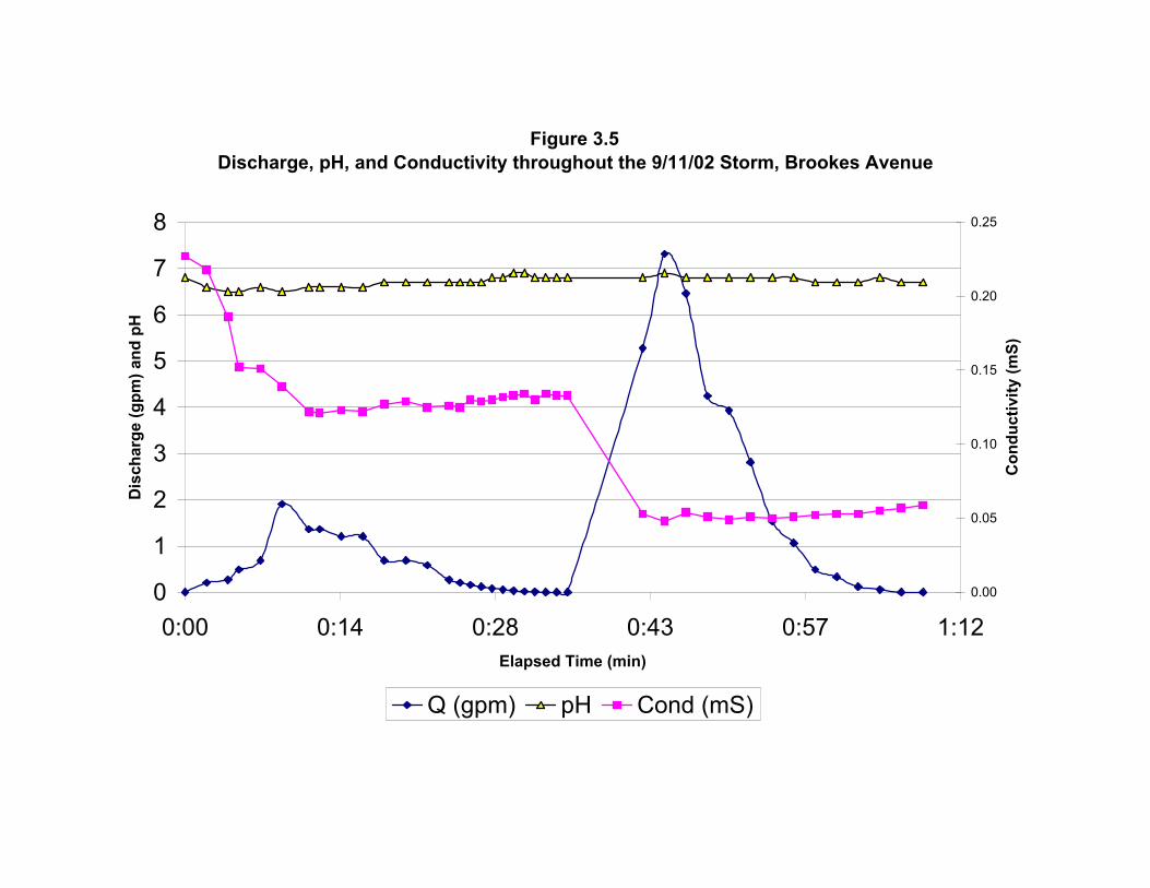
Figure 3.5Discharge, pH, and Conductivity throughout the 9/11/02 Storm, Brookes Avenue

0

1

2

3

4

5

6

7

8

0:00 0:14 0:28 0:43 0:57 1:12Elapsed Time (min)

Dis

char

ge (g

pm) a

nd p

H

0.00

0.05

0.10

0.15

0.20

0.25

Con

duct

ivity

(mS)

Q (gpm) pH Cond (mS)

Figure 3.6 Calcium Concentration and Discharge with Runoff Discharge, Perkins weir 9/11/02

0

1000

2000

3000

4000

5000

6000

0 5 10 15 20 25 30 35 40 45

Elapsed Time (min)

Cal

cium

Dis

char

ge (m

g/m

in)

0

10

20

30

40

50

60

Run

off D

isch

arge

(gpm

) and

Cal

cium

C

once

ntra

tion

(ppm

)

Calcium (mg/min) Q (gpm)Ca (ppm)

Chapter 4 – Discussion

Changes in Steady State Infiltration Rates with Remediation Treatment

Statistical analysis showed that, only one month after remediation, treatments

consisting of compost, aeration, and seeding resulted in significantly greater infiltration

rates than prior to remediation (Table 3.1). Such an increase was not seen after one month

for either fenced plots or plots that received only aeration and seeding. Thus, to

significantly and rapidly improve steady-state infiltration rates for compacted soils

remediation must include both aeration and composting. However, after six months, sites

which received only aeration and seeding did show a significantly greater infiltration rate

than prior to remediation and the mean infiltration rates over these aerated sites were not

significantly different than those which received compost and aeration. This suggests that

with six months time, aeration and seeding may be just as effective in improving

infiltration rates as the combined treatment of aeration, composting, and seeding.

Improvement was seen in mean infiltration rates for all treatments over time (Table 3.1).

There are several explanations for these results. It has been shown that

immediately after intense aeration, such as tilling, hydraulic conductivity is decreased

because pore structure is lost (Coutadeur, 2002). This also has an effect on vegetative

growth. Passioura, (2002), states that plant growth may be reduced in extremely loose

soil. Immediately after aeration, it is likely that the soil did not have a healthy pore

structure. Over time vegetative growth was seen, soil settling occurred, and the soil was

probably reworked by earthworms. This resulted in a healthier pore structure yielding the

infiltration improvement that was seen for all remediation treatments with time. I believe

32

that composting added nutrients, which sped the growth of vegetative cover, improving

pore structure (Coutadeur, 2002), resulting in the earlier improvements in infiltration

rates over these sites.

After 6 months, sites which were only fenced had mean steady state infiltration

rates of 8 cm/h, suggesting more than a 6 cm/h improvement over infiltration rates

measured prior to fencing (Table 3.1). This result suggests that allowing compacted soils

to stand alone with out further compaction allows their permeability to improve. This

improvement must be the result of increased pore structure created by encroaching

vegetation, such as the vine-like weeds that were seen on the cook control site, as well as

macro-pore structures left by worm burrows.

After six months, sites which received aeration had mean infiltration rates more

than 13 cm/h. Considering that precipitation in Burlington is typically of less intensity

than these infiltration rates (http://www.erh.noaa.gov/btv/html/climo2.shtml) we can

assume that the amount of runoff over remediated sites would be very little during most

rain events in Burlington.

Changes in Normalized Suspended Sediment Loading with Remediation Treatment

After one month, significant improvements (drops) in normalized mean

suspended sediment production were seen on sites that were both aerated and composted

(Table 3.3). Statistically significant improvements were not seen over fenced or aerated

sites until six months after remediation. I attribute these differences in large part to

vegetative cover. After one month, vegetation was denser over the sites that received

compost as treatment, while other sites had sparse grass cover. In general, vegetation

33

prevents erosion, thus reducing suspended sediment production (Harden, 1992). After 6

months, sites that were aerated had dense grass cover and significantly less suspended

sediment was produced compared to before remediation.

It is not clear what causes the significant drop in suspended sediment production

on the sites that received just fencing. There was some vegetative cover over these

surfaces; however, this cover was very superficial and patchy, so I do not believe this can

account for all of the reduction in suspended sediment production. I also observed the

presence of many pebbles covering the surface of the control plots. Reid and Dunne

(1984) noted that abandoned dirt roads produced 130% less suspended sediment than

active dirt roads. I believe that a similar result is seen here; there was less erosion over

these fenced sites because their isolation allowed an armored layer of pebbles to develop

and minimize the detachment of fine particles.

Prior to remediation, the mean mass of suspended sediment produced per square

meter per cm of rainfall was 30.5 grams. Six months after remediation, mean normalized

production of suspended sediment was less than 2 grams from fenced sites and less than

0.5 grams over aerated and composted sites. This indicates that through active

remediation and an effort to protect greenspace from disturbance, total suspended

sediment production could be drastically reduced throughout Burlington.

Changes in contaminant concentrations from the remediation test plots

Only three of the eight EPA priority pollutants that I tested for were detected

regularly within the remediation plot runoff: Cu, Cr, and Zn (Table 3.4). However, these

contaminants and the other EPA priority pollutants were detected in very low

34

concentrations, well below their respective EPA MCL, and usually below the mean from

the NURP (1981). Concentrations of these eight contaminants were similar to the

concentrations seen in the study by Zartman (2001).

The elements that were most prevalent in the remediation runoff were Ca, K, Mg,

Na, and Si (Table 3.5). Sodium concentrations showed a steady decrease over time for

every site and testing round (Table 3.4, Figure 3.2). This makes sense since sodium is

relatively soluble and its most likely source is deicing salt applied in the winter (Table

4.1). Over the summer, without a major source, its concentrations would naturally fall as

it is washed out of the soils. I thought that I would see significant differences in chemical

concentrations associated with remediation treatment differences; however, no significant

chemical trends were associated with different treatments. Table 4.1 lists potential

stormwater sources for the elements found in the remediation plots.

Stormwater flow, pH, and Conductivity analysis

Stormwater runoff flux responded rapidly on the rising and falling hydrograph

limbs to increases and decreases in precipitation intensity through the 9/11/02 and

9/27/02 events (Figure 3.3 and Figure 3.4). My runoff verses rainfall analysis for the two

drainage basins over the two storm events did not produce the data that I expected.

Drainage basin delineations and land cover mapping (Figures 1.2 and 1.3 and Tables 1.1

and 1.2) suggested that the Perkins Parking lot and the Brookes Avenue drainage basins

were covered by 85% and 75% impermeable surfaces, respectively, yet only 5-31%

runoff was measured during the storm events using the weirs (Tables 3.6 through 3.9).

The weirs were clearly inadequate for measuring storm flow from these drainage basins;

35

through significant portions of both the small and large storm events, the weirs were over

topped (Tables 3.5 through 3.8). There are several other factors that may have contributed

to this underestimate. There was water detention in puddles on the south side of the

Perkins drainage basin. Also, greenspace was located down hill from impermeable areas

at Perkins and Brookes Avenue (Figure 1.1 and 1.2). This greenspace could have acted as

an infiltrating buffer for some of the runoff that was generated over the impermeable

surfaces. This probably mattered more for the short, low-intensity storm because I

suspect that during the high intensity, twelve-hour storm, runoff may have been generated

over the green space. Weir design flaws including the lack of a uniform substrate leading

to the weir and the lack of adequate height behind the weir may have also created errors

within the runoff calculations.

Conductivity measurements showed dilution with increasing stormwater flux; that

is, conductivity decreased when stormwater discharge increased because similar numbers

of ions were dispersed in a greater volume of water (Figure 3.5). Rainwater pH was

generally more acidic than stormwater pH suggesting that buffering of rainwater acidity

occurred rapidly once flow moved over the drainage basins. Decreases in stormwater pH

were associated with increases in rainfall intensity (Figure 3.5 and Appendix A). This

must be because of a dilution of alkalinity ions in a greater volume of acidic runoff

(Lepori, 2003). The opposite is also true; increases in pH are associated with lesser

rainfall intensities and stormwater flow because there are more alkaline ions to buffering

fewer acidic ions.

36

Stormwater Chemistry

Similar to the conductivity results, elements decreased in concentration (diluted)

when stormwater discharge increased (Figure 3.6). Over entire storm events, chemical

concentrations decreased per stormwater volume (Figure 3.6). This is important because

it indicates that the first flush of stormwater has the highest concentrations of

contaminants. Eight of the contaminants on the EPA’s priority pollutant list were

detected in stormwater samples (Ag, As, Cd, Cr, Cu, Ni, Pb, and Zn). In most samples

these concentrations were low (Table 3.10 through Table 3.13), but in samples 3P1, 3B1,

3B2, and 3B3, the EPA MCL for lead was exceeded (Appendix B). The presence of these

dissolved metals may be attributed to the sources listed in table 4.1 including corrosion of

metal from cars, insecticides, gasoline combustion, tire degradation, oil, and natural

sources such as the dissolution of soils.

Lead concentrations during the September 27th, 2002 storm event were much

higher than during the short duration September 11th storm. At Perkins Parking lot, the

first flush of stormwater contained 0.033 ppm of lead, more than twice the 0.015 MCL

for lead and at Brookes Avenue lead was detected in 93% of the samples, with the first

three samples above the MCL (Appendix B). It is very significant that three samples were

above the MCL; this represents more than an hour of storm flow that had lead

concentrations above the MCL. What is really intriguing about these lead concentrations

is that they were so high during the 9/27/02 storm and so low during the 9/11/02 storm

(Appendix B). Before the September 11th storm, there was a significant period of time

without rainfall while before the September 27th storm there had been several recent and

significant rainfalls. Thus, the higher lead concentrations are likely not due to runoff

37

dissolving particulates on the basin surface, but perhaps due to the flushing of soil water.

This hypothesis suggests that the soil over these sites may have high levels of lead. This

is a real possibility especially in the Brookes drainage basin, which includes old houses.

Runoff from the roof tops and sidewalls of old houses has elevated lead concentrations

because of the lead in the materials that cover these surfaces (Steinberg, in progress). It is

likely that particles of lead paint are common throughout the soils surrounding these

houses, resulting in elevated lead concentrations within the soil; thus, lead may dissolve

and flush out during storm events when the soils are saturated with water. These findings

for lead are counter to the generally assumed paradigm that longer periods without

rainfall are periods of deposition in urban environments and this results in higher

concentrations of contaminants during a storm’s first flush (Stephenson, 1981).

With rational method discharge calculations, I was able to estimate total dissolved

chemical loads for the two drainage basins and storm events. I then normalized these data

by unit depth of rainfall and drainage basin area, which allowed me to compare total

loading between drainage basins and over two storms (Table 3.14). These data showed

that there was more intense chemical loading for all chemicals during the short duration

9/11/02 storm than the long 9/27/02 storm except for Ag and Pb. This general trend is

consistent with the paradigm that a greater period of dry deposition will result in a greater

flushing of contaminants. The deviations seen in lead and silver may be associated with

soil water flushing during the second, saturated storm.

38

Table 4.1Typical Stormwater Sources for the 17 Elements Analyzed

Element SourcesAg photo processingAl natural erosion, alloysAs product of fossil fuel combustion, herbicidesCa deicing salts, natural erosionCd fertilizers, insecticidesCr corrosion of alloys, electroplating wastes, natural erosion

Cu corrosion of plumbing, metal platings, and brake linings, fungicides, and insecticides

Fe rusting metalsK natural erosion

Mg natural erosionNa deicing saltsNi product of fossil fuel combustion, batteriesP detergents, excrement, fertilizers, atmosphere

Pb tire wear, car exhaust, oil, batteriesSi natural erosionSr natural erosionZn Component of automobile tires, oils, and greese, ingredient in road salt

Sources: NURP (1983), Whipple (1983), Dennison (1996)

Chapter 5 -Conclusions

Remediation consisting of aeration, composting, seeding and a barrier to prevent

further compaction appears to be the best method for restoring soil permeability and

reducing suspended sediment production from compacted soils. This treatment was able

to significantly improve infiltration rates of compacted soils from about 1.5 cm/h to more

than 15 cm/h, a ten-fold increase. This treatment was also able reduce suspended

sediment production from 34 (g/m2)/ (cm of rain) to less than 0.5 (g/m2)/ (cm of rain), a

seven 70 fold decrease. Burlington and other cities could significantly reduce stormwater

runoff and suspended sediment production by remediating compacted soils and protecting

existing greenspace.

I learned many things about the difficulty of obtaining accurate stormwater flow

measurements directly from the street, but by estimating stormwater flow using the

rational runoff method I was able to make several important observations. During the

September 11th rain event, which was preceded by a long period of dry deposition, more

intense loading occurred over both Perkins Parking lot and Brookes Avenue than during

the September 27th storm, which was preceded by a rainy period. This agrees with

previous research that suggests chemical loading may be more intense after long periods

of dry deposition. Perkins Parking lot contributed more intense loading of the elements

Al, As, Ca, Cr, Cu, Fe, Mg, Ni, Si, and Sr, while Brookes Avenue had more intense

loadings of K, Na, P, Pb, and Zn (Table 3.14). These data suggests that the two basins

may have different dissolved load chemical sources.

During the 9/27/02 storm, Brookes Avenue and Perkins Parking lot experienced

an initial flux of lead in concentrations exceeding the MCL for drinking water. Initial

39

flushing, such as this, was observed in both storms with all the elements measured

(Appendix B and C). However, even with dilution, significant contaminant loading

occurred throughout the storm events and increased with increasing stormwater discharge

(Figure 3.7). This indicates that contaminant loading continues throughout urban runoff

events, even though elemental concentrations may decrease due to dilution.

Future research is needed to better understand both aspects my study. Clearly

more research is needed to explain the differences in sources of chemical loading

between the two drainage basins. The most important research would analyze soil

chemistry on the remediation test plots and at select places throughout the two studied

drainage basins. This would enable one to narrow down the potential sources of the

contaminants detected in significant concentrations in the runoff. It might also be

interesting to test smaller drainage basins with more uniform land cover; this would also

be useful in narrowing down contaminant sources within the runoff. Further event

sampling would also be helpful to determine differences in chemical loading between the

drainage basins and storm types. I believe that the remediation test plot study should be

followed up to check on the condition of the test plots. Another interesting idea would be

to remove the barriers around some of the remediation test plots and replace some of the

barriers with shrubs, then to record what effect this has. How fast would greenspace be

lost over non-protected surfaces? Do natural, more aesthetically pleasing barriers provide

enough protection for the greenspace?

40

References: 1999 LMNO Engineering, Research, and Software, Ltd. (All Rights Reserved) “V- Notch Weir Discharge Calculator and Equations.” http://www.lmnoeng.com/Weirs/vweir.htm Bhaduri, Budhendra and others (2000). “Assessing Watershed-Scale, Long Term Hydrologic Impacts of Land-Use Change Using a GIS-NPS Model.” Environmental Management, Vol. 26, No. 6, pp. 643-658. Booth, Derek B. (1991). “Urbanization and the Natural Drainage System-Impacts, Solutions, and Prognoses.” The Northwest Environmental Journal vol. 7 pp 93-118 Booth, Derek B. and Jackson, C. Rhett (October 1997) “Urbanization of Aquatic Systems: Degradation Thresholds, Stormwater Detection, and the Limits of Mitigation.” Journal of the American Water Resources Association vol. 33, no. 5 Burlington Bay Project, School of Natural Resources, University of Vermont. http://snr.uvm.edu/bbay/ Coutadeur C., Y. Coquet, and J. Rodger Estrade. (2002) “Variation of Hydraulic Conductivity in a Tilled Soil.” European Journal of Soil Science. vol. 53 pp. 619-628. Dennison, Mark S. Stormwater Discharges: Regulatory Compliance and Best Management Practices. Lewis Publishers, New York, 1996. Driver and Tasker, “Techniques for Estimation of Storm-Runoff Loads, Volumes, and Selected Constituent Concentrations in Urban Watersheds in the United States.” US Geological Survey Water-Supply Paper 2363, Library of Congress Cataloging in Publication Data, 1990. Encyclopedia Britannica (2003). http://www.britannica.com/ Harden, Carol P. (1992) “Incorporating Roads and Footpaths in Watershed- Scale Hydrologic and Soil Erosion Models” Physical Geography, vol. 13, no. 4, pp. 368-385 Helliwell, P.R. Urban Storm Drainage, Proceedings of the International conference held at the University of South Hampton, April 1978. John Wiley & Sons. New York, 1978. Kurfis J., Bierman P., Nichols K., Persico L., Mellilo P. (2001). Green University town succumbs to blacktop: Quantifying the increase in impermeable surfaces and

41

runoff through time. (7), A-179 Geological Society of America, Abstracts with Programs (National). http://geology.uvm.edu/morphwww/urbanhydro/hydro2001.html http://geology.uvm.edu/morphwww/urbanhydro/kurfisstudy.html Lake Champlain Basin Program http://www.lcbp.org/ Lepori, Fabio, Alberto Barbieri, and S.J. Ormerod. (2003) “Causes of Episodic Acidification in Alpine Streams” Freshwater Biology vol. 48 pp. 175-189. McGee, Megan (2003) “What is her title?” University of Vermont senior research Mellilo, Paul “Urban Infiltration Study” http://geology.uvm.edu/morphwww/urbanhydro/paulm/urbanhydrohomepage.html Mulvany, T.J. (1851) “On the use of self-registering rain and flood gauges, in making observations of the relations of rainfall and flood discharges in a given catchment.” Dublin, Ireland: Transactions and Minutes of the Proceedings of the Institute of Civil Engineers of Ireland. Session 1850-1, 4(2). National Weather Service, Burlington, VT. http://www.erh.noaa.gov/btv/html/climo2.shtml

Nichols et al., in review, “Quantifying Land use and Urban Runoff Changes Through Service-Learning Hydrology Projects”, Journal of Geoscience Education.

Nix, Stephan J. Urban Stormwater Modeling and Simulation. Lewis Publishers. Boca Raton, FL, 1994. Passioura J.B. (2002) “Soil Conditions and Plant Growth” Plant, Cell and Environment vol. 25 pp. 311-315. Pit, Robert (1999) “Infiltration through disturbed urban soils and compost-amended soil effects on Runoff Quality and Quantity.” Environmental Protection Agency. www.epa.gov/ednnrmrl/reports/SR00016/ Reid, Leslie M. and Dunne, Thomas (1984) “Sediment Production from Forest Road Surfaces.” Water Resources Research, vol. 20, no. 11, pp 1753-1761 Results of the Nationwide Urban Runoff Program (1982). Environmental Protection Agency. Number 841S83101. Richard G., I. Cousin, J.F. Sillon, A. Braund, and J. Guerif (2001) “Effects of compaction on the porosity of a silty soil: influence on unsaturated hydraulic properties.” European Journal of Soil Science vol. 52 pp. 49-58.

42

Stephenson, D. Developments in Water Science: Stormwater Hydrology and Drainage. Elsevier Scientific Publishing Company. New York, 1981. Stickney, Michaela, Colleen Hickey and Roland Hoerr, (2001), “Lake Champlain Basin Program: Working Together Today for Tomorrow.” Lakes and Reservoirs Research and Management, vol. 6 pp. 217-223. Steinberg, Laura J. and Myers, Ridgley P. (In Progress) “Quantifying Urban Non-Point Sources of Lead for use in TMDL Computations” Tulane University, Department of Civil and Environmental Engineering. Whipple, William, et al. Stormwater Management in Urbanizing Areas. Prentice Hall, Inc. Englewood, Cliffs, New Jersey. 1983. Wije, Suran, University of Texas at Austin (January 1998). “Loss of Greenspace in the City of Austin from the Grant of Minor Variances.” http://www.utexas.edu/depts/grg/ustudent/gcraft/fall96/wije/projects/zoning.html Zartman, R.E., R.H. Ramsey III, A. Huang. (Summer 2001) “Variability of Total Dissolved elements in Stormwater Runoff” Journal of Soil and Water conservation, v56 p263

43

Appendices

44

Appendix A1: Perkins Parking Lot Flow Data 9/11/02

height to V-notch (cm) 5.6

Sample Time Elapsed Time Stage (cm) Head (cm) Q (gpm) Cond (mS) pH1P1 7:41 AM 0:00:00 5.6 0.0 0.21 0.229 6.92P1 7:42 AM 0:01:00 8.5 2.9 3.34 0.213 7.23P1 7:43 AM 0:02:00 10 4.4 9.24 0.206 7.34P1 7:44 AM 0:03:00 11 5.4 15.27 0.189 7.35P1 7:45 AM 0:04:00 13 7.4 33.21 0.176 7.36P1 7:45 AM 0:04:30 13.5 7.9 39.04 0.162 7.47P1 7:46 AM 0:05:00 14 8.4 45.44 0.140 7.48P1 7:46 AM 0:05:30 14.2 8.6 48.16 0.138 7.49P1 7:47 AM 0:06:00 14.5 8.9 52.43 0.137 7.4

10P1 7:47 AM 0:06:30 14.6 9.0 53.90 0.108 7.411P1 7:48 AM 0:07:00 14.7 9.1 55.39 0.114 7.412P1 7:49 AM 0:08:00 14.7 9.1 55.39 0.102 7.413P1 7:49 AM 0:08:30 14.7 9.1 55.39 0.102 7.514P1 7:50 AM 0:09:30 14.6 9.0 53.90 0.093 7.615P1 7:51 AM 0:10:00 14.4 8.8 50.98 0.091 7.516P1 7:52 AM 0:11:00 14.3 8.7 49.56 0.088 7.517P1 7:52 AM 0:11:30 14.3 8.7 49.56 0.087 7.518P1 7:53 AM 0:12:00 14.2 8.6 48.16 0.083 7.519P1 7:53 AM 0:12:30 14.1 8.5 46.79 0.084 7.520P1 7:54 AM 0:13:30 14.1 8.5 46.79 0.082 7.621P1 7:56 AM 0:15:00 13.9 8.3 44.12 0.079 7.522P1 7:58 AM 0:17:00 13.6 8.0 40.27 0.077 7.523P1 8:00 AM 0:19:00 13.2 7.6 35.48 0.072 7.524P1 8:02 AM 0:21:00 12.5 6.9 27.94 0.069 7.525P1 8:04 AM 0:23:00 12.3 6.7 25.99 0.070 7.426P1 8:06 AM 0:25:00 11.8 6.2 21.46 0.066 7.427P1 8:09 AM 0:28:00 11.6 6.0 19.80 0.064 7.428P1 8:12 AM 0:31:00 11.1 5.5 15.98 0.064 7.429P1 8:14 AM 0:33:00 10.6 5.0 12.64 0.063 7.530P1 8:17 AM 0:36:00 9.9 4.3 8.73 0.066 7.431P1 8:20 AM 0:39:00 9.3 3.7 6.05 0.068 7.432P1 8:23 AM 0:42:00 9 3.4 4.92 0.070 7.4

Rain: 0.017 4.9

Appendix A2: Brookes Avenue Flow Data 9/11/02

Height to V: 3.5 cm

Sample Time Elapsed Time Stage (cm) Head (cm) Q (gpm) Cond (mS) pH1B1 7:47:30 0:00 3.5 0.0 0.000 0.227 6.82B1 7:49:30 0:02 4.4 0.9 0.210 0.218 6.63B1 7:51:30 0:04 4.5 1.0 0.268 0.186 6.54B1 7:52:30 0:05 4.8 1.3 0.492 0.152 6.55B1 7:54:30 0:07 5.0 1.5 0.688 0.151 6.66B1 7:56:30 0:09 5.8 2.3 1.908 0.139 6.57B1 7:59:00 0:11 5.5 2.0 1.364 0.122 6.68B1 8:00:00 0:12 5.5 2.0 1.364 0.121 6.69B1 8:02:00 0:14 5.4 1.9 1.207 0.123 6.6

10B1 8:04:00 0:16 5.4 1.9 1.207 0.122 6.611B1 8:06:00 0:18 5.0 1.5 0.688 0.127 6.712B1 8:08:00 0:20 5.0 1.5 0.688 0.129 6.713B1 8:10:00 0:22 4.9 1.4 0.585 0.125 6.714B1 8:12:00 0:24 4.5 1.0 0.268 0.126 6.715B1 8:13:00 0:25 4.4 0.9 0.210 0.125 6.716B1 8:14:00 0:26 4.3 0.8 0.161 0.130 6.717B1 8:15:00 0:27 4.2 0.7 0.119 0.129 6.718B1 8:16:00 0:28 4.1 0.6 0.085 0.130 6.819B1 8:17:00 0:29 4.0 0.5 0.057 0.132 6.820B1 8:18:00 0:30 3.9 0.4 0.036 0.133 6.921B1 8:19:00 0:31 3.8 0.3 0.020 0.134 6.922B1 8:20:00 0:32 3.7 0.2 0.010 0.130 6.823B1 8:21:00 0:33 3.6 0.1 0.003 0.134 6.824B1 8:22:00 0:34 3.5 0.0 0.000 0.133 6.825B1 8:23:00 0:35 3.5 0.0 0.000 0.133 6.826B1 8:30:00 0:42 7.0 3.5 5.280 0.053 6.827B1 8:32:00 0:44 7.5 4.0 7.316 0.048 6.928B1 8:34:00 0:46 7.3 3.8 6.453 0.054 6.829B1 8:36:00 0:48 6.7 3.2 4.245 0.051 6.830B1 8:38:00 0:50 6.6 3.1 3.929 0.049 6.831B1 8:40:00 0:52 6.2 2.7 2.810 0.051 6.832B1 8:42:00 0:54 5.6 2.1 1.534 0.050 6.833B1 8:44:00 0:56 5.3 1.8 1.061 0.051 6.834B1 8:46:00 0:58 4.8 1.3 0.492 0.052 6.735B1 8:48:00 1:00 4.6 1.1 0.333 0.053 6.736B1 8:50:00 1:02 4.2 0.7 0.119 0.053 6.737B1 8:52:00 1:04 4.0 0.5 0.057 0.055 6.838B1 8:54:00 1:06 3.6 0.1 0.003 0.057 6.739B1 8:56:00 1:08 3.5 0.0 0.000 0.059 6.7

Rain: 0.017 4.9

Appendix A3: Perkins Parking Lot Flow Data 9/27/02

Height to V: 4.5 cm

Sample Time Elapsed Time Stage (cm) Head (cm) Q (gpm) Cond (uS) pH1P3 11:36:00 0:00:00 4.5 0.0 0.000 178.90 6.92P3 11:56:00 0:20:00 7.2 2.7 2.810 128.90 6.63P3 12:06:00 0:30:00 7.5 3.0 3.628 109.40 6.84P3 12:33:00 0:57:00 9.1 4.6 10.302 69.00 75P3 13:10:00 1:34:00 10.0 5.5 15.980 46.70 7.16P3 13:30:00 1:54:00 9.7 5.2 13.921 37.20 7.27P3 13:50:00 2:14:00 10.5 6.0 19.798 33.60 7.38P3 14:10:00 2:34:00 9.6 5.1 13.272 37.20 7.39P3 14:30:00 2:54:00 8.1 3.6 5.655 45.30 7.3

10P3 15:03:00 3:27:00 10.8 6.3 22.327 34.00 7.211P3 15:23:00 3:47:00 9.7 5.2 13.921 34.40 7.312P3 15:41:00 4:05:00 11.1 6.6 25.042 28.00 7.313P3 16:00:00 4:24:00 11.3 6.8 26.956 27.50 7.214P3 16:23:00 4:47:00 8.8 4.3 8.732 39.80 7.315P3 16:48:00 5:12:00 7.7 3.2 5.245 45.60 7.316P3 17:20:00 5:44:00 9.5 5.0 12.642 39.60 7.317P3 17:48:00 6:12:00 10.2 5.7 17.448 23.10 7.318P3 18:13:00 6:37:00 14.3 9.8 66.553 19.20 7.119P3 18:32:00 6:56:00 13.1 8.6 48.162 20.10 720P3 19:00:00 7:24:00 12.5 8.0 40.273 22.20 7.121P3 19:25:00 7:49:00 15.8 11.3 94.735 17.00 7.222P3 19:48:00 8:12:00 15.2 10.7 82.746 14.70 7.323P3 20:25:00 8:49:00 12.6 8.1 41.529 20.00 7.224P3 20:45:00 9:09:00 14.7 10.2 73.489 16.10 7.225P3 21:05:00 9:29:00 13.7 9.2 56.912 19.50 726P3 21:35:00 9:59:00 12.0 7.5 34.335 20.00 727P3 22:15:00 10:39:00 13.4 8.9 52.428 18.90 7.128P3 22:40:00 11:04:00 11.0 6.5 24.116 25.50 7.129P3 23:15:00 11:39:00 9.2 4.7 10.860 33.70 7.130P3 23:50:00 12:14:00 7.8 3.3 4.575 45.20 7.131P3 0:14:00 12:38:00 6.5 2.0 1.364 55.80 7.2

R1 12:53 PM 14.3 7.3R2 1:53 PM 10.3 6.2R3 3:07 PM 8.4 6.1R4 3:55 PM 10.5 6.3R5 5:10 PM 4.3 6R6 6:00 PM 8.4 7.1R7 6:22 PM 6.7 6.4R8 6:44 PM 7 5.9R9 7:13 PM 12.6 6.1

R10 7:30 PM 5.8 6.2R11 8:17 PM 3.5 6.1R12 8:40 PM 5.3 6.2R13 9:15 PM 3.1 6.1R14 10:15 PM 8.5 6.2R15 11:15 PM 4.4 5.9R16 24:14:00 n/a 6.3

Appendix A4: Brookes Avenue Flow Data 9/27/02

Height to V: 4.3

Sample Time Elapsed Time Stage (cm) Head (cm) Q (gpm) Cond (uS) pH1B3 12:36 PM 0:00:00 4.3 0.0 0.000 135.8 6.62B3 12:48 PM 0:12:00 5.0 0.7 0.119 95.3 6.73B3 1:11 PM 0:35:00 6.0 1.7 0.926 92 6.74B3 1:32 PM 0:56:00 6.6 2.3 1.908 57.1 7.15B3 1:53 PM 1:17:00 6.8 2.5 2.333 40.2 7.26B3 2:18 PM 1:42:00 5.5 1.2 0.408 48.8 7.17B3 2:45 PM 2:09:00 4.6 0.3 0.020 110.8 7.18B3 3:07 PM 2:31:00 6.8 2.5 2.333 38.8 7.29B3 3:31 PM 2:55:00 7.0 2.7 2.810 32.8 7.2

10B3 3:51 PM 3:15:00 7.0 2.7 2.810 29.9 7.311B3 4:14 PM 3:38:00 6.2 1.9 1.207 27.1 7.212B3 4:40 PM 4:04:00 5.6 1.3 0.492 55.4 7.213B3 5:10 PM 4:34:00 5.5 1.2 0.408 66.3 7.114B3 5:30 PM 4:54:00 8.7 4.4 9.238 33.2 7.315B3 6:00 PM 5:24:00 8.0 3.7 6.047 24.9 7.216B3 6:22 PM 5:46:00 9.4 5.1 13.272 11.2 6.917B3 6:45 PM 6:09:00 7.0 2.7 2.810 25.4 6.918B3 7:10 PM 6:34:00 9.8 5.5 15.980 14.4 6.819B3 7:35 PM 6:59:00 11.5 7.2 31.041 11.1 720B3 8:10 PM 7:34:00 7.8 3.5 5.280 16.2 7.121B3 8:35 PM 7:59:00 8.5 4.2 8.243 16.5 7.122B3 9:10 PM 8:34:00 11.4 7.1 29.987 11.3 723B3 9:32 PM 8:56:00 9.2 4.9 12.030 15.5 6.924B3 10:02 PM 9:26:00 11.2 6.9 27.945 11.3 725B3 10:25 PM 9:49:00 8.0 3.7 6.047 18.1 6.926B3 10:45 PM 10:09:00 7.2 2.9 3.342 21.3 6.827B3 11:10 PM 10:34:00 6.1 1.8 1.061 23.8 6.828B3 11:30 PM 10:54:00 4.9 0.6 0.085 45.5 6.8

R1 12:53 14.3 7.3R2 13:53 10.3 6.2R3 15:07 8.4 6.1R4 15:55 10.5 6.3R5 17:10 4.3 6R6 18:00 8.4 7.1R7 18:22 6.7 6.4R8 18:44 7 5.9R9 19:13 12.6 6.1

R10 19:30 5.8 6.2R11 20:17 3.5 6.1R12 20:40 5.3 6.2R13 21:15 3.1 6.1R14 22:15 8.5 6.2R15 23:15 4.4 5.9R16 24:14:00 n/a 6.3

Appendix B1: Perkins Parking Lot Samples: Chemical Concentrations (ppm) for 9/11/02 Rain Event Sample Ag Al As Ca Cd Cr Cu Fe K Mg Na Ni P Pb Si Sr Zn

0.001 0.002 0.004 0.0001 0.0004 0.001 0.002 0.0006 0.01 0.0002 0.004 0.002 0.008 0.004 0.001 0.0002 3E-04 Detection Limit0.1 0.2 0.01 NA 0.005 0.1 1 0.3 NA NA 20 0.1 NA 0.015 NA 4 2 MCL

1P1 BDL 0.126 BDL 39.960 0.001 0.007 0.033 0.047 3.886 1.751 11.430 0.012 0.059 BDL 0.464 0.113 0.1272P1 BDL 0.115 0.004 37.330 BDL 0.007 0.031 0.033 3.238 1.615 6.519 0.009 0.016 BDL 0.381 0.105 0.0873P1 BDL 0.108 BDL 34.160 BDL 0.006 0.035 0.028 3.150 1.651 3.158 0.008 0.124 BDL 0.485 0.096 0.0954P1 BDL 0.112 BDL 31.880 BDL 0.004 0.034 0.032 2.276 1.427 5.556 0.007 0.010 BDL 0.316 0.090 0.1115P1 BDL 0.096 BDL 29.060 BDL 0.005 0.028 0.026 2.235 1.306 7.696 0.008 0.019 BDL 0.331 0.083 0.0766P1 BDL 0.095 BDL 28.320 BDL 0.004 0.023 0.023 1.728 1.228 6.100 0.010 0.012 BDL 0.302 0.079 0.0687P1 BDL 0.090 BDL 24.040 BDL 0.003 0.025 0.024 1.478 1.254 4.546 0.007 0.014 BDL 0.273 0.068 0.0838P1 BDL 0.094 BDL 24.880 0.002 0.005 0.027 0.034 1.312 1.091 5.937 0.008 BDL BDL 0.301 0.071 0.0999P1 BDL 0.091 BDL 24.690 BDL 0.003 0.024 0.023 1.283 1.031 4.477 0.005 0.012 BDL 0.279 0.070 0.096

10P1 BDL 0.077 BDL 19.050 BDL 0.003 0.019 0.015 1.076 0.854 3.246 0.004 0.013 BDL 0.231 0.054 0.08511P1 BDL 0.091 BDL 20.660 BDL 0.003 0.020 0.023 1.398 1.097 3.420 0.005 0.014 BDL 1.129 0.058 0.08612P1 BDL 0.097 BDL 20.160 BDL 0.002 0.012 0.047 0.732 1.080 2.609 BDL 0.014 BDL 0.252 0.064 0.02813P1 BDL 0.076 BDL 18.460 BDL 0.003 0.015 0.015 0.961 0.805 2.613 0.003 0.026 BDL 0.233 0.051 0.05514P1 BDL 0.066 BDL 16.640 BDL 0.003 0.015 0.011 0.701 0.700 3.595 0.002 BDL BDL 0.210 0.047 0.05715P1 BDL 0.073 BDL 16.050 0.001 0.003 0.013 0.018 0.739 0.663 2.406 0.004 0.010 BDL 0.214 0.046 0.06516P1 0.002 0.067 BDL 15.630 BDL 0.002 0.012 0.009 0.781 0.636 2.256 0.002 0.011 BDL 0.200 0.045 0.04717P1 BDL 0.069 0.005 15.110 BDL 0.001 0.013 0.011 0.821 0.619 2.214 BDL BDL BDL 0.189 0.044 0.09118P1 0.003 0.076 0.004 14.420 BDL 0.002 0.014 0.010 0.779 0.599 2.113 BDL BDL BDL 0.190 0.041 0.03619P1 0.003 0.075 BDL 14.590 BDL 0.002 0.012 0.010 0.768 0.597 2.088 BDL 0.012 BDL 0.190 0.042 0.03520P1 BDL 0.072 BDL 14.720 BDL 0.002 0.012 0.009 0.778 0.584 2.046 BDL BDL BDL 0.187 0.043 0.03521P1 BDL 0.062 BDL 13.380 BDL 0.002 0.013 0.008 0.837 0.538 2.119 BDL 0.012 BDL 0.147 0.039 0.03022P1 BDL 0.069 BDL 13.150 0.001 0.003 0.013 0.016 0.828 0.522 2.003 BDL BDL BDL 0.197 0.039 0.03023P1 0.002 0.062 BDL 12.420 BDL 0.002 0.012 0.008 0.811 0.509 1.828 BDL BDL BDL 0.181 0.037 0.02924P1 BDL 0.064 0.004 11.930 BDL 0.003 0.009 0.007 0.772 0.477 1.737 BDL BDL BDL 0.191 0.035 0.02725P1 0.001 0.057 BDL 11.650 BDL 0.003 0.011 0.007 0.862 0.465 1.809 BDL 0.012 BDL 0.171 0.035 0.03126P1 BDL 0.057 0.004 11.440 BDL 0.002 0.011 0.005 0.854 0.441 1.656 BDL BDL BDL 0.178 0.034 0.03027P1 0.001 0.064 0.005 11.220 0.001 0.003 0.009 0.016 0.785 0.441 1.563 BDL 0.012 BDL 0.195 0.034 0.02728P1 0.003 0.059 BDL 11.230 BDL 0.002 0.010 0.006 0.834 0.427 1.638 BDL 0.017 BDL 0.187 0.033 0.02529P1 0.002 0.055 BDL 11.080 BDL 0.001 0.009 0.005 0.847 0.419 1.529 BDL 0.013 BDL 0.186 0.033 0.02530P1 0.003 0.055 BDL 11.510 BDL 0.002 0.011 0.005 0.827 0.447 1.616 BDL 0.011 BDL 0.198 0.034 0.03331P1 0.002 0.055 BDL 11.850 BDL 0.002 0.010 0.005 0.814 0.464 1.636 BDL 0.011 BDL 0.213 0.036 0.03632P1 BDL 0.063 0.005 11.930 0.002 0.003 0.010 0.057 0.818 0.497 1.934 BDL 0.020 BDL 0.237 0.038 0.081

Rain BDL BDL BDL 1.37 BDL BDL 0.011 BDL 0.32 0.20 2.35 BDL BDL BDL 0.02 0.008 0.005Footnote: Rain was not filtered before acidification; Thus, concentrations in the rain may be elevated

Appendix B2: Brookes Ave Samples: Chemical Concentrations (ppm) for 9/11/02Sample Name Ag Al As Ca Cd Cr Cu Fe K Mg Na Ni P Pb Si Sr Zn

Detection Limit 0.001 0.002 0.004 0.0001 0.0004 0.001 0.002 0.0006 0.01 0.0002 0.004 0.002 0.008 0.004 0.001 0.0002 0.0003MCL or Other 0.1 0.2 0.01 NA 0.005 0.1 1 0.3 NA NA 20 0.1 NA 0.015 NA 4 2

1B1 BDL 0.105 BDL 35.170 0.001 0.004 0.021 0.020 6.719 1.606 10.550 0.003 0.282 0.005 0.372 0.113 0.1752B1 BDL 0.090 BDL 25.750 BDL 0.003 0.030 0.012 9.547 1.774 11.720 0.002 0.409 BDL 0.211 0.084 0.1773B1 BDL 0.086 BDL 18.970 BDL 0.002 0.024 0.012 9.067 1.825 11.200 BDL 0.395 BDL 0.227 0.062 0.1524B1 BDL 0.063 BDL 13.330 BDL 0.002 0.016 0.014 7.827 1.734 13.440 BDL 0.309 BDL 0.269 0.043 0.1125B1 BDL 0.061 BDL 11.660 BDL 0.002 0.016 0.013 6.491 1.442 13.920 BDL 0.175 BDL 0.267 0.038 0.0886B1 0.003 0.055 BDL 10.020 BDL 0.002 0.014 0.014 5.590 1.227 13.740 BDL 0.115 BDL 0.255 0.033 0.0747B1 0.003 0.048 BDL 8.518 BDL 0.002 0.011 0.016 4.647 1.019 12.130 BDL 0.132 BDL 0.159 0.028 0.0558B1 0.001 BDL BDL BDL BDL BDL BDL 0.003 BDL BDL BDL BDL BDL BDL BDL BDL BDL9B1 BDL 0.063 BDL 8.187 0.001 0.005 0.011 0.026 4.263 0.955 13.110 BDL 0.116 0.007 0.187 0.028 0.096

10B1 BDL 0.050 BDL 8.122 BDL 0.003 0.010 0.022 4.036 0.901 13.080 BDL 0.093 BDL 0.220 0.027 0.06711B1 BDL 0.050 BDL 8.249 BDL 0.003 0.012 0.017 3.918 0.896 13.600 BDL 0.095 BDL 0.160 0.027 0.04512B1 0.002 0.051 BDL 8.025 BDL 0.003 0.009 0.014 3.745 0.867 14.160 BDL 0.097 0.004 0.149 0.027 0.07913B1 0.002 0.043 BDL 7.873 BDL 0.003 0.013 0.013 3.523 0.864 16.570 BDL 0.057 BDL 0.220 0.027 0.09414B1 0.002 0.047 BDL 7.555 BDL 0.003 0.010 0.016 3.446 0.780 14.780 BDL 0.070 BDL 0.196 0.026 0.06415B1 0.002 0.045 BDL 7.334 BDL 0.002 0.015 0.020 3.356 0.763 15.130 BDL 0.066 BDL 0.181 0.024 0.05116B1 0.002 0.046 BDL 7.152 BDL 0.001 0.014 0.018 3.242 0.761 15.530 BDL 0.053 BDL 0.190 0.024 0.08517B1 0.001 0.043 BDL 7.226 BDL 0.002 0.012 0.014 3.312 0.752 16.120 BDL 0.033 BDL 0.217 0.025 0.05118B1 BDL 0.046 BDL 7.301 BDL 0.003 0.010 0.015 3.180 0.736 15.530 BDL 0.043 BDL 0.213 0.025 0.04419B1 BDL 0.048 BDL 7.418 BDL 0.002 0.010 0.022 3.109 0.754 15.940 BDL 0.021 0.004 0.202 0.026 0.07020B1 0.002 0.046 BDL 9.223 BDL 0.002 0.007 0.014 3.036 0.773 15.750 BDL 0.020 0.005 0.197 0.040 0.03421B1 0.001 0.044 BDL 7.664 BDL 0.002 0.007 0.016 3.114 0.774 16.120 BDL 0.046 BDL 0.231 0.027 0.02822B1 0.002 0.044 BDL 7.904 BDL 0.003 0.047 0.058 3.146 0.785 16.200 BDL 0.046 BDL 0.629 0.080 0.04023B1 BDL BDL BDL 8.403 BDL 0.003 0.011 0.012 3.301 0.794 15.800 BDL 0.033 BDL 0.227 0.032 0.03524B1 0.002 BDL BDL 8.321 BDL 0.002 0.015 0.016 3.417 0.825 16.260 BDL 0.035 BDL 0.215 0.031 0.07225B1 0.001 BDL 0.005 8.349 BDL 0.001 0.016 0.012 3.423 0.798 16.380 BDL 0.023 BDL 0.192 0.030 0.04026B1 0.002 BDL BDL 4.346 BDL BDL 0.007 0.012 1.840 0.440 4.526 BDL 0.080 BDL 0.109 0.016 0.04827B1 BDL BDL BDL 3.668 0.001 0.002 0.005 0.021 2.147 0.426 3.529 BDL 0.111 BDL 0.125 0.013 0.03128B1 BDL BDL BDL 4.145 BDL BDL 0.005 0.010 2.639 0.456 3.884 BDL 0.138 BDL 0.114 0.013 0.02429B1 0.002 BDL BDL 3.934 BDL 0.001 0.004 0.009 2.398 0.445 3.511 BDL 0.121 BDL 0.093 0.013 0.02630B1 BDL BDL BDL 3.700 BDL BDL 0.006 0.007 2.328 0.421 3.587 BDL 0.106 BDL 0.065 0.012 0.04031B1 0.002 BDL BDL 3.731 BDL BDL 0.009 0.006 2.277 0.429 3.896 BDL 0.108 BDL 0.063 0.013 0.03432B1 BDL BDL BDL 3.518 0.001 0.002 0.006 0.017 1.988 0.382 4.049 BDL 0.089 BDL 0.078 0.012 0.02533B1 BDL BDL BDL 3.649 BDL 0.002 0.005 0.005 2.046 0.401 4.124 BDL 0.086 BDL 0.083 0.012 0.03934B1 0.003 BDL BDL 3.680 BDL 0.002 0.006 0.009 2.090 0.402 4.112 BDL 0.099 BDL 0.082 0.012 0.04235B1 0.002 BDL BDL 3.749 BDL 0.003 0.025 0.014 2.479 0.427 4.994 BDL 0.086 BDL 0.111 0.013 0.04536B1 0.004 BDL BDL 3.540 BDL 0.002 0.007 0.010 2.047 0.412 4.437 BDL 0.087 BDL 0.083 0.012 0.03937B1 BDL BDL BDL 3.888 BDL 0.001 0.007 0.008 2.099 0.426 4.580 BDL 0.089 BDL 0.063 0.013 0.06438B1 BDL BDL BDL 4.374 BDL 0.002 0.008 0.002 2.166 0.436 4.593 BDL 0.094 BDL 0.098 0.015 0.06039B1 0.001 BDL BDL 4.575 0.002 0.004 0.012 0.023 2.144 0.461 4.801 BDL 0.084 BDL 0.121 0.017 0.115Rain BDL BDL BDL 1.365 BDL BDL 0.011 BDL 0.322 0.200 2.345 BDL BDL BDL 0.018 0.008 0.005

Footnote: rain was not filtered before acidication; thus, concentrations within the rain may be elevated

Appendix B3: Perkins Parking Lot Samples: Chemical Concentrations (ppm) for 9/27/02 Rain Event

Sample Ag Al As Ca Cd Cr Cu Fe K Mg Na Ni P Pb Si Sr ZnDetection Limit 0.001 0.002 0.004 0.0001 0.0004 0.001 0.002 0.0006 0.01 0.0002 0.004 0.002 0.008 0.004 0.001 0.0002 0.0003MCL or Other 0.1 0.2 0.01 NA 0.005 0.1 1 0.3 NA NA 20 0.1 NA 0.015 NA 4 2

3P1 BDL 0.128 0.006 33.22 0.0009 0.008 0.034 0.034 2.67 0.119 0.39 0.003 0.056 0.0325 0.131 0.005 0.0693P2 BDL 0.114 0.004 25.58 BDL 0.005 0.019 0.024 1.37 1.166 9.68 0.009 0.096 BDL 3.441 0.083 0.0583P3 BDL 0.102 0.004 20.76 BDL 0.004 0.014 0.015 1.15 0.872 5.45 0.005 0.037 BDL 2.090 0.064 0.0563P4 BDL 0.090 0.004 13.04 BDL 0.003 0.011 0.026 0.76 0.724 4.25 0.003 0.039 0.0042 1.613 0.053 0.0483P5 BDL 0.059 0.004 9.14 BDL 0.003 0.013 0.008 0.51 0.446 2.50 BDL 0.030 0.0047 0.836 0.035 0.0473P6 0.002 0.071 BDL 7.20 BDL 0.002 0.014 0.011 0.60 0.288 1.48 BDL 0.013 BDL 0.440 0.024 0.0373P7 BDL 0.065 BDL 7.01 BDL 0.002 0.012 0.002 0.45 0.222 0.91 BDL 0.024 BDL 0.248 0.019 0.0343P8 0.002 0.069 0.006 7.78 BDL 0.002 0.006 0.002 0.39 0.201 0.70 BDL 0.011 0.0046 0.201 0.018 0.0233P9 BDL 0.078 0.005 9.46 BDL 0.002 0.012 0.007 0.48 0.209 0.64 BDL 0.017 BDL 0.229 0.020 0.016

3P10 BDL 0.061 0.005 6.61 BDL 0.002 0.012 0.001 0.37 0.267 0.85 BDL 0.013 BDL 0.289 0.024 0.0183P11 0.002 0.062 BDL 7.30 BDL 0.002 0.004 BDL 0.33 0.169 0.59 BDL 0.015 BDL 0.160 0.016 0.0133P12 0.008 0.063 BDL 5.92 0.0015 0.004 0.007 0.005 0.27 0.187 0.61 BDL 0.014 BDL 0.173 0.018 0.0103P13 0.006 0.052 BDL 5.70 BDL 0.003 0.009 BDL 0.26 0.164 0.50 BDL 0.015 BDL 0.137 0.016 0.0123P14 0.004 0.062 BDL 8.16 BDL 0.003 0.003 BDL 0.28 0.142 0.45 BDL BDL BDL 0.112 0.015 0.0093P15 0.006 0.072 BDL 9.49 BDL 0.002 0.003 BDL 0.31 0.193 0.58 BDL 0.017 BDL 0.168 0.021 0.0103P16 0.007 0.061 BDL 8.21 BDL 0.002 0.006 BDL 0.29 0.244 0.65 BDL 0.018 BDL 0.226 0.024 0.0123P17 0.007 0.040 BDL 4.75 0.002 0.005 0.010 0.010 0.10 0.204 0.59 BDL BDL BDL 0.172 0.021 0.0133P18 0.005 0.029 BDL 3.78 BDL 0.002 0.011 BDL 0.25 0.122 0.57 BDL BDL 0.0043 0.113 0.013 0.0113P19 0.006 0.028 BDL 4.23 BDL 0.002 BDL BDL 0.14 0.090 0.48 BDL BDL BDL 0.063 0.010 0.0283P20 0.007 0.031 BDL 4.66 BDL 0.002 BDL BDL 0.15 0.097 0.29 BDL BDL BDL 0.061 0.017 0.0173P21 0.003 0.025 BDL 2.91 BDL 0.002 0.003 BDL 0.55 0.098 0.26 BDL BDL BDL 0.067 0.012 0.0123P22 0.002 0.021 BDL 3.02 BDL 0.003 BDL BDL 0.12 0.072 0.35 BDL 0.110 BDL 0.105 0.008 0.0063P23 0.006 0.034 0.004 4.20 0.001 0.003 BDL BDL 0.14 0.063 0.22 BDL BDL BDL 0.057 0.008 0.0033P24 0.007 0.031 BDL 3.61 BDL 0.002 0.002 BDL 0.12 0.095 0.26 BDL BDL BDL 0.089 0.011 0.0093P25 0.005 0.032 BDL 4.12 BDL 0.001 0.011 BDL 0.17 0.098 0.20 BDL BDL BDL 0.056 0.009 0.0313P26 0.005 0.032 BDL 4.49 BDL 0.002 0.002 BDL 0.14 0.115 0.30 BDL BDL BDL 0.113 0.011 0.0163P27 0.004 0.031 BDL 3.91 BDL 0.002 0.005 BDL 0.22 0.121 0.24 BDL BDL BDL 0.078 0.012 0.0123P28 0.007 0.041 0.004 5.48 0.0014 0.003 BDL BDL 0.15 0.120 0.40 BDL BDL BDL 0.091 0.011 0.0113P29 BDL 0.044 BDL 7.62 BDL 0.001 BDL BDL 0.17 0.116 0.32 BDL BDL BDL 0.090 0.015 0.0103P30 BDL 0.054 BDL 10.19 BDL 0.001 BDL BDL 0.20 0.141 0.35 BDL BDL BDL 0.099 0.019 0.0093P31 0.001 0.070 BDL 11.25 BDL 0.001 0.002 BDL 0.26 0.199 0.49 BDL BDL BDL 0.148 0.026 0.012

Footnote: Rain data is on Appendix B5

Appendix B4: Brookes Ave. Samples: Chemical Concentrations (ppm) for 9/27/02

Sample Name Ag Al As Ca Cd Cr7 Cu Fe K Mg Na Ni P Pb Si Sr ZnDetection Limit 0.001 0.002 0.004 0.0001 0.0004 0.001 0.002 0.0006 0.01 0.0002 0.004 0.002 0.008 0.004 0.001 0.0002 0.0003MCL or Other 0.1 0.2 0.01 NA 0.005 0.1 1 0.3 NA NA 20 0.1 NA 0.015 NA 4 2

3B1 0.002 0.093 BDL 11.750 BDL 0.002 0.011 0.074 2.330 0.797 4.881 BDL BDL BDL 0.511 0.081 0.0583B2 0.005 0.077 0.005 7.492 0.001 0.004 0.009 0.070 1.841 1.023 18.270 BDL 0.071 0.015 0.313 0.036 0.1033B3 0.005 0.072 BDL 11.730 BDL 0.001 0.007 0.027 1.414 0.713 14.350 BDL 0.056 0.017 0.270 0.023 0.0543B4 0.004 0.052 BDL 7.189 BDL 0.001 0.011 0.020 1.300 0.564 7.886 BDL 0.052 0.016 0.191 0.032 0.0373B5 0.005 0.039 BDL 5.190 BDL 0.004 0.004 0.009 0.947 0.396 4.030 BDL 0.034 0.008 0.119 0.019 0.0493B6 0.004 0.045 BDL 6.435 BDL 0.002 0.005 0.015 0.886 0.333 2.559 BDL 0.028 0.009 0.090 0.014 0.0263B7 0.002 0.077 BDL 18.560 BDL 0.001 0.003 0.007 0.857 0.358 3.012 BDL 0.024 0.007 0.103 0.018 0.0403B8 0.003 0.057 BDL 5.703 0.002 0.002 0.005 0.025 0.780 0.457 3.903 BDL 0.032 0.008 0.144 0.051 0.0613B9 0.005 0.031 BDL 4.486 BDL 0.002 0.003 BDL 0.686 0.307 2.328 BDL 0.020 0.011 0.110 0.017 0.044

3B10 0.003 0.030 BDL 4.089 BDL 0.002 0.002 0.001 0.781 0.274 1.918 BDL 0.031 0.007 0.077 0.013 0.0313B11 0.005 0.024 BDL 3.559 BDL 0.001 0.002 BDL 0.698 0.246 1.460 BDL 0.026 0.006 0.065 0.011 0.0233B12 BDL 0.046 BDL 8.348 BDL 0.001 0.005 BDL 0.625 0.250 1.649 BDL 0.014 0.005 0.063 0.010 0.0203B13 0.003 0.054 BDL 10.070 BDL 0.001 0.004 0.002 0.553 0.298 2.387 BDL 0.019 0.005 0.087 0.024 0.0213B14 0.007 0.041 0.005 4.564 0.002 0.006 0.013 0.015 0.725 0.331 3.229 BDL BDL 0.005 0.113 0.029 0.0223B15 0.003 0.027 BDL 3.884 BDL 0.002 0.003 BDL 0.558 0.259 1.608 BDL 0.016 0.007 0.082 0.014 0.0263B16 0.004 0.030 BDL 3.630 BDL 0.015 0.040 0.009 1.610 0.195 0.813 BDL 0.016 0.006 0.044 0.011 0.0143B17 0.005 0.027 BDL 3.891 BDL 0.003 0.006 BDL 0.624 0.240 1.859 0.004 0.013 0.005 0.057 0.013 0.0503B18 0.002 0.018 BDL 2.173 BDL BDL 0.002 BDL 0.407 0.191 0.840 BDL 0.015 0.006 0.037 0.011 0.0143B19 0.003 0.025 BDL 1.863 0.002 0.004 0.003 0.009 0.384 0.115 0.407 BDL BDL 0.004 0.027 0.006 0.0083B20 0.003 0.020 BDL 2.568 BDL BDL 0.007 BDL 0.356 0.111 0.271 BDL 0.013 0.007 0.048 0.007 0.0073B21 0.001 0.016 BDL 2.445 BDL 0.001 BDL BDL 0.225 0.129 0.440 BDL BDL 0.005 0.025 0.008 0.0103B22 0.001 0.016 BDL 1.766 BDL 0.001 0.005 BDL 0.295 0.131 0.653 BDL 0.011 0.004 0.024 0.007 0.0093B23 0.003 0.023 BDL 3.351 BDL 0.001 0.005 0.001 0.350 0.102 0.355 BDL BDL 0.006 0.026 0.005 0.0293B24 0.005 0.025 BDL 1.836 0.002 0.003 0.002 0.007 0.301 0.138 0.403 BDL BDL BDL 0.025 0.007 0.0303B25 0.004 0.026 BDL 3.076 BDL 0.002 0.004 BDL 0.306 0.104 0.273 BDL 0.013 0.006 0.045 0.006 0.0203B26 0.002 0.024 BDL 3.495 BDL 0.002 0.004 BDL 0.264 0.137 0.418 BDL BDL BDL 0.024 0.008 0.0243B27 BDL 0.027 BDL 4.065 BDL 0.001 0.002 BDL 0.271 0.170 0.535 BDL BDL 0.005 0.031 0.011 0.0263B28 0.004 0.037 BDL 7.736 BDL 0.002 0.002 BDL 0.272 0.191 0.768 BDL 0.010 0.005 0.035 0.012 0.020

Footnote: Rain data is on Appendix B5

Appendix B5: 9/27/02 Rain Data, Chemical Concentrations (ppm)

Sample Name Ag Al As Ca Cd Cr Cu Fe K Mg Na Ni P Pb Si Sr ZnDetection Limit 0.001 0.002 0.004 0.0001 0.0004 0.001 0.002 0.0006 0.01 0.0002 0.004 0.002 0.008 0.004 0.001 0.0002 0.0003MCL or Other 0.1 0.2 0.01 NA 0.005 0.1 1 0.3 NA NA 20 0.1 NA 0.015 NA 4 2

9/27 R1 0.002 0.036 BDL 1.457 BDL BDL 0.076 0.011 0.579 5.044 12.690 BDL 0.968 0.001 1.099 0.135 0.1219/27 R2 0.001 0.050 BDL 0.953 BDL BDL 0.035 0.023 0.374 0.239 0.796 0.006 0.027 0.004 0.034 0.007 0.1369/27 R3 BDL 0.061 BDL 0.989 BDL 0.005 0.032 0.039 0.275 0.084 0.587 BDL BDL 0.018 0.029 0.005 0.0719/27 R4 0.002 0.111 BDL 1.385 BDL 0.001 0.020 0.098 0.412 0.080 0.428 0.003 0.017 0.010 0.040 0.005 0.1439/27 R5 0.005 0.138 BDL 0.383 BDL 0.001 0.013 0.120 0.196 0.115 0.502 BDL 0.024 0.018 0.088 0.009 0.0889/27 R6 0.005 0.562 0.006 3.627 0.002 0.004 0.034 0.353 0.245 0.065 0.192 BDL BDL 0.006 0.126 0.002 0.0289/27 R7 0.005 0.234 BDL 1.236 BDL 0.006 0.019 0.237 0.189 0.256 0.273 0.005 0.098 0.087 0.358 0.021 0.0679/27 R8 0.006 0.104 BDL 0.677 BDL 0.005 0.028 0.083 0.299 0.111 0.224 0.051 0.105 0.048 0.165 0.007 0.0429/27 R9 0.008 0.505 BDL 2.351 0.002 0.034 0.040 0.330 0.605 0.067 0.391 0.003 0.017 0.022 0.076 0.004 0.036

9/27 R10 0.008 0.610 BDL 1.732 0.001 0.005 0.019 0.388 0.148 0.308 0.738 0.010 0.051 0.087 0.376 0.021 0.0909/27 R11 0.007 0.262 BDL 1.495 BDL 0.002 0.011 0.159 0.047 0.660 0.153 0.006 0.082 0.086 0.583 0.011 0.0509/27 R12 0.008 0.331 BDL 1.374 BDL 0.002 0.012 0.263 0.165 0.140 0.054 BDL 0.027 0.040 0.210 0.006 0.0209/27 R13 0.006 0.202 BDL 0.880 BDL 0.002 0.009 0.172 0.061 0.202 0.168 BDL 0.034 0.094 0.278 0.009 0.0339/27 R14 0.008 0.267 BDL 1.412 0.002 0.006 0.073 0.188 0.215 0.075 0.053 BDL 0.027 0.041 0.140 0.004 0.0259/27 R15 0.004 0.085 BDL 0.633 BDL 0.003 0.012 0.080 0.084 0.203 0.285 0.011 0.021 0.057 0.178 0.008 0.0979/27 R16 0.004 0.127 BDL 1.435 0.001 0.006 0.020 0.124 0.284 0.220 1.063 BDL BDL 0.006 0.050 0.024 0.018

Footnote: Rain was not filtered before acidication; thus, concentrations may be elevated

Appendix B6 Remediation Test Plot Chemical Concentrations (ppm)

Sample Name Date Ag As Cd Cr Cu Ni Pb Zn Al Ca Fe K Mg Na P Si SrDetection Limit 0.001 0.004 0.0004 0.001 0.002 0.002 0.004 0.0003 0.002 0.0001 0.0006 0.01 0.0002 0.004 0.008 0.001 0.0002

MCL1 0.1 0.01 0.005 0.1 1 0.1 0.015 2 0.2 NA 0.3 NA NA 20 NA NA 4Cook 1 5/20/02 BDL BDL BDL 0.002 0.010 BDL BDL 0.005 0.090 42.41 0.001 3.22 5.17 18.61 0.350 0.76 0.163

(Control Site) 6/10/02 BDL 0.005 BDL 0.002 0.002 BDL BDL 0.021 0.092 44.63 BDL2 2.31 4.46 16.26 0.378 0.78 0.19311/12/02 BDL BDL BDL 0.002 0.008 BDL 0.004 0.010 0.117 51.37 BDL 10.96 0.23 1.93 BDL 0.17 0.029

Cook 2 6/10/02 BDL 0.004 BDL 0.002 0.003 BDL BDL 0.044 0.080 33.22 0.001 2.84 4.31 12.16 0.411 0.84 0.13711/12/02 BDL 0.006 BDL 0.001 0.005 BDL BDL 0.032 0.106 34.99 0.003 10.71 5.02 16.04 0.851 0.89 0.209

Cook 3 6/10/02 BDL 0.004 0.001 0.002 0.005 BDL BDL 0.084 0.106 56.48 0.018 4.29 4.84 12.08 0.447 1.22 0.22711/12/02 BDL BDL BDL 0.003 0.006 BDL BDL 0.069 0.119 83.74 BDL 16.08 4.41 9.57 0.684 1.11 0.123

Cook4 6/10/02 BDL 0.006 BDL BDL BDL BDL BDL 0.025 0.090 50.77 BDL 1.61 4.74 12.45 0.335 0.86 0.23411/12/02 BDL BDL BDL 0.004 0.012 BDL BDL 0.049 0.134 254.10 BDL 16.00 4.54 9.24 0.679 1.08 0.290

Cook 5 6/10/02 BDL 0.004 BDL 0.002 BDL BDL BDL 0.045 0.104 77.04 0.006 3.72 5.00 13.43 0.393 0.86 0.28911/12/02 BDL BDL BDL 0.005 0.005 BDL BDL 0.129 0.119 66.33 BDL 9.32 8.81 17.17 0.586 1.26 0.894

Cook 6 6/10/02 BDL 0.005 BDL 0.002 0.003 BDL BDL 0.062 0.104 96.32 0.012 14.41 5.18 14.25 1.047 0.98 0.32211/12/02 BDL BDL BDL 0.004 0.015 BDL BDL 0.029 0.148 78.47 0.046 25.82 4.86 12.79 0.630 0.92 0.245

Cook 7 6/10/02 0.002 0.016 BDL 0.003 0.045 0.004 BDL 0.139 0.248 57.72 0.365 88.32 5.86 36.11 5.562 2.53 0.17211/12/02 BDL BDL BDL 0.003 0.003 BDL BDL 0.042 0.119 83.83 BDL 9.56 7.63 13.73 3.197 1.71 0.232

Cook 8 6/10/02 BDL BDL BDL 0.003 0.002 BDL BDL 0.038 0.002 93.67 BDL 6.04 5.44 14.99 0.471 0.83 0.33711/12/02 BDL BDL 0.002 0.004 0.006 BDL BDL 0.052 0.136 73.31 0.013 11.05 4.35 8.95 1.109 0.82 0.127

Fleming 5/16/02 BDL BDL BDL 0.002 0.016 BDL BDL 0.012 0.100 29.89 0.020 3.87 3.92 24.93 0.373 1.27 0.1796/14/02 BDL BDL BDL 0.002 0.012 BDL BDL 0.065 0.088 105.20 0.138 35.71 5.63 24.67 3.558 1.48 0.329

Torrey 5/16/02 BDL 0.006 BDL 0.002 0.021 BDL BDL 0.355 0.089 24.86 0.006 3.05 3.82 18.93 0.297 0.87 0.1226/14/02 NA NA NA NA NA NA NA NA NA NA NA NA NA NA NA NA NA

Old Mill 5/17/02 BDL 0.006 0.001 0.002 0.004 BDL BDL 0.010 0.108 31.78 0.010 1.91 4.29 12.68 0.250 0.72 0.1616/17/02 NA NA NA NA NA NA NA NA NA NA NA NA NA NA NA NA NA

Footnote: Simulation prinkling blanks are not included because they were not filtered before acidificationAlso, one representative pre-remediation cook sample (5/20/02) was obtained.

Cook control, changes in Ca, Mg, Na, K, Al, P, Si, and Sr concentrations

0

10

20

30

40

50

60

4/14/2002 5/24/2002 7/3/2002 8/12/2002 9/21/2002 10/31/2002 12/10/2002

Date

Ca.

Mg,

Na,

and

K (d

ashe

d lin

es) C

hem

ical

Co

ncen

trat

ion

(ppm

)

0.0

0.1

0.2

0.3

0.4

0.5

0.6

0.7

0.8

0.9

Al,

P, S

i, Sr

(sol

id li

nes)

Con

cent

ratio

ns (p

pm)

Ca Mg Na K Al P Si Sr

Cook 2 Changes in Al, Ca, K, Mg, Na, P, Si, and Sr Concentrations (ppm)

0

5

10

15

20

25

30

35

40

45

4/14/2002 5/24/2002 7/3/2002 8/12/2002 9/21/2002 10/31/2002 12/10/2002

Date

Ca,

K, M

g, a

nd N

a (d

ashe

d lin

e) c

once

ntra

tons

(ppm

)

0.0

0.1

0.2

0.3

0.4

0.5

0.6

0.7

0.8

0.9

1.0

Al,

P, S

i, an

d Sr

(sol

id li

nes)

conc

entr

atio

ns (p

pm)

Ca K Mg Na Al P Si Sr

Cook 3 Changes in Al, Ca, K, Mg, Na, P, Si, and Sr Concentrations (ppm)

0

10

20

30

40

50

60

70

80

90

4/14/2002 5/24/2002 7/3/2002 8/12/2002 9/21/2002 10/31/2002 12/10/2002

Date

Ca,

K, M

g, a

nd N

a (d

ashe

d lin

e) c

once

ntra

tions

(ppm

)

0.0

0.2

0.4

0.6

0.8

1.0

1.2

1.4

Al,

P, S

i, an

d Sr

(sol

id li

ne)

conc

entr

atio

ns (p

pm)

Ca K Mg Na Al P Si Sr

Cook 4 Changes in Al, Ca, K, Mg, Na, P, Si, and Sr Concentrations (ppm)

0

10

20

30

40

50

60

4/14/2002 5/24/2002 7/3/2002 8/12/2002 9/21/2002 10/31/2002 12/10/2002Date

Ca,

K, M

g, a

nd N

a (d

ashe

d lin

e) c

once

ntra

tions

(ppm

)

0.0

0.2

0.4

0.6

0.8

1.0

1.2

Al,

P, S

i, an

d Sr

(sol

id li

ne)

conc

entr

atio

ns (p

pm)

Ca K Mg Na Al P Si Sr

Appendix C: Cook 1- 4 Al, Ca, K, Mg, Na, P, Si, and Sr Chemical Changes

Cook 5 Changes in Al, Ca, K, Mg, Na, P, Si, and Sr Concentrations (ppm)

0

10

20

30

40

50

60

70

80

90

04/14/02 05/24/02 07/03/02 08/12/02 09/21/02 10/31/02 12/10/02

Date

Ca,

K, M

g, a

nd N

a (d

ashe

d lin

e) c

once

ntra

tions

(ppm

)

0.0

0.2

0.4

0.6

0.8

1.0

1.2

1.4

Al,

P, S

i, an

d Sr

(sol

id li

nes)

conc

entr

atio

ns (p

pm)

Ca K Mg Na Al P Si Sr

Cook 6 Changes in Al, Ca, K, Mg, Na, P, Si, and Sr Concentrations (ppm)

0

20

40

60

80

100

120

04/14/02 05/24/02 07/03/02 08/12/02 09/21/02 10/31/02 12/10/02

Date

Ca,

K, M

g, a

nd N

a (d

ashe

d lin

e) c

once

ntra

tions

(ppm

)

0.0

0.2

0.4

0.6

0.8

1.0

1.2

Al,

P, S

i, an

d Sr

(sol

id li

nes)

conc

entr

atio

ns (p

pm)

Ca K Mg Na Al P Si Sr

Cook 7 Changes in Al , Ca, K, Mg, Na, P, Si, and Sr Concentrations (ppm)

0

10

20

30

40

50

60

70

80

90

100

04/14/02 05/24/02 07/03/02 08/12/02 09/21/02 10/31/02 12/10/02

Date

Ca,

K, M

g, a

nd N

a (d

ashe

d lin

es) c

once

ntra

tion

(ppm

)

0.0

1.0

2.0

3.0

4.0

5.0

6.0

Al,

P, S

i, an

d Sr

(sol

id li

nes)

conc

entr

atio

ns (p

pm)

Ca K Mg Na Al P Si Sr

Cook 8 Changes in Al, Ca, K, Mg, Na, P, Si, and Sr Concentrations (ppm)

0

10

20

30

40

50

60

70

80

90

100

4/14/2002 5/24/2002 7/3/2002 8/12/2002 9/21/2002 10/31/2002 12/10/2002

Date

Ca,

K, M

g, a

nd N

a (d

ashe

d lin

es) c

once

ntra

tions

(ppm

)

0.0

0.2

0.4

0.6

0.8

1.0

1.2

Al,

P, S

i, an

d Sr

(sol

id li

nes)

conc

entr

atio

ns (p

pm)

Ca K Mg Na Al P Si Sr

Appendix C: Cook 5- 8 Al, Ca, K, Mg, Na, P, Si, and Sr Chemical Changes

Cook plots change in zinc concentration

0.00

0.02

0.04

0.06

0.08

0.10

0.12

0.14

0.16

04/14/02 05/24/02 07/03/02 08/12/02 09/21/02 10/31/02 12/10/02

Date

Che

mic

al C

once

ntra

tion

(ppm

)

Zn2138 Cook1 Zn2138 Cook2 Zn2138 Cook3 Zn2138 Cook4 Zn2138 Cook5 Zn2138 Cook6 Zn2138 Cook7 Zn2138 Cook8

Cook plots change in copper concentration

0

0.005

0.01

0.015

0.02

0.025

0.03

0.035

0.04

0.045

0.05

05/04/02 05/24/02 06/13/02 07/03/02 07/23/02 08/12/02 09/01/02 09/21/02 10/11/02 10/31/02 11/20/02 12/10/02

Date

Che

mic

al C

once

ntra

tion

(ppm

)

Cu3247 Cook1 Cu3247 Cook2 Cu3247 Cook3 Cu3247 Cook4 Cu3247 Cook5 Cu3247 Cook6Cu3247 Cook7 Cu3247 Cook8

Cook plots change in chromium concentration

0.0000

0.0020

0.0040

0.0060

04/14/02 05/24/02 07/03/02 08/12/02 09/21/02 10/31/02 12/10/02

Date

Che

mic

al C

once

ntra

tion

(ppm

)

Cr2677 Cook 1 Cr2677 Cook 2 Cr2677 Cook 3 Cr2677 Cook 4 Cr2677 Cook 5 Cr2677 Cook 6Cr2677 Cook 7 Cr2677 Cook 8

Appendix C: Cook plot comparison of Zn, Cu, and Cr chemical changes

Appendix C: Perkins Parking lot, 9/11/02:Concentrations and Chemical Discharges

Priority Pollutant Discharge and Runoff Discharge, Perkins Weir, 9/11/02

0

10

20

30

40

50

60

0 10 20 30 40 50

Elapsed Time (min)

Disc

harg

e (g

pm) a

nd

Zinc

Con

cent

ratio

n (p

pm)

0

1

2

3

4

5

6

Cr, C

u, N

i Con

cent

ratio

n (p

pm)

Q (gpm) Zinc (mg/min) Chromium (mg/min)Copper (mg/min) Nickle (mg/min)

Discharge of Al, Fe, K, Mg, P, Si, and Sr (mg/min) with Runoff Discharge (gpm), Perkins Weir,

9/11/02

0

50

100

150

200

250

300

350

0 10 20 30 40 50

Elapsed Time (min)

Si, M

g, a

nd K

D

isch

arge

(mg/

min

)

0

10

20

30

40

50

60

Run

off D

isch

arge

(g

pm) a

nd A

l, Fe

, P,

and

Sr d

isch

arge

(m

g/m

in)

Silica (mg/min) Magnesium (mg/min) Potassium (mg/min) Q (gpm)Strontium (mg/min) Phosporus(mg/min) Iron (mg/min) Aluminum (mg/min)

Priority Pollutant Concentration with Runoff Discharge, Perkins Weir, 9/11/02

0.00

10.00

20.00

30.00

40.00

50.00

60.00

0 10 20 30 40 50

Elapsed Time (min)

Dis

char

ge (g

pm)

0

0.02

0.04

0.06

0.08

0.1

0.12

0.14

Con

cent

ratio

n (p

pm)

Q (gpm) Zn Cu Cr Ni

Figure 33: Al, Fe, K, Mg, P, Si, and Sr Concentrations (ppm) and Runoff Discharge

(gpm), Perkins Weir, 9/11/02

0

10

20

30

40

50

60

0 10 20 30 40 50

Elapsed Time (min)

Disc

harg

e (g

pm) a

nd K

and

Mg

Conc

entra

tions

(ppm

)

0

0.2

0.4

0.6

0.8

1

1.2

Al, F

e, P

, Si, a

nd S

r co

ncen

trtio

ns (p

pm)

Mg K Q (gpm) Sr Si P Fe Al

Appendix C: Brookes Avenue, 9/11/02:Concentrations and Chemical Discharges

Figure 38: Ca, K, Mg, and Na Discharge (mg/min) with Stormwater Discharge (gpm), Brookes

Avenue, 9/11/02

020406080

100120

0 20 40 60 80

Elapsed Time (min)

Ca,

K, M

g an

d N

a D

isch

arge

(m

g/m

in)

0

2

4

6

8

Stot

mw

ater

D

isch

arge

(g

pm)

Calcium Discharge (mg/min) Potassium Discharge (mg/min)Magnesium Discharge (mg/min) Sodium Discharge (mg/min)Q (gpm)

Figure 37: Ca, K, Mg, and Na Concentration (ppm) and Runoff Discharage (gpm), Brookes Avenue

Weir, 9/11/02

0

1

2

3

4

5

6

7

8

0 20 40 60 80

Elapsed Time (min)

Dis

char

ge (g

pm)

0

5

10

15

20

25

30

35

40

Ca,

K, M

g, a

nd N

a co

ncen

trat

ions

(ppm

)

Q (gpm) Ca K Mg Na

Figure 39: Cr, Cu, and Zn Discharge (mg/min) with Stormwater Discharge (gpm), Brookes Avenue, 9/11/02

012345678

0 20 40 60 80

Elapsed Time

Disc

harg

e (gp

m)

0.00

0.20

0.40

0.60

0.80

1.00

1.20

Cr, C

u, a

nd Z

n Di

scha

rge

(mg/

min)

Q (gpm) Chromium Discharge (mg/min)Copper Discharge (mg/min) Zinc Discharge (mg/min)

Figure 42: Al, Fe, P, Si, and Sr Concentrations (ppm) with Stormwater Discharge (gpm), Brookes

Avenue, 9/11/02

0

2

4

6

8

0 20 40 60 80

Elapsed Time (min)

Dis

char

ge (g

pm)

0

0.1

0.2

0.3

0.4

0.5

0.6

0.7

Al,

Fe, P

, Si,

and

Sr

Con

cent

ratio

ns

(ppm

)

Q (gpm) Al Fe P Si Sr

Figure 41: Al, Fe, P, Si, and Sr Discharge (mg/min) and Stormwater Discharge (gpm), Brookes Avenue, 9/11/02

0

2

4

6

8

0 20 40 60 80

Elapsed Time (min)

Dis

char

ge (g

pm)

0.0

1.0

2.0

3.0

4.0

Al,

Fe, P

, Si,

and

Sr

Dis

char

ge (m

g/m

in)

Q (gpm) Aluminum Discharge (mg/min) Iron Discharge (mg/min)Phosphorus Discharge (mg/min) Silica Discharge (mg/min) Strontium Discharge (mg/min)

Figure 40: Cr, Cu, and Zn Concentrations (ppm) and Stormwater Discharge (gpm), Brookes

Avenue, 9/11/02

0.0001.0002.0003.0004.0005.0006.0007.0008.000

0 20 40 60 80

Elapsed Time (min)

Dis

char

ge (g

pm)

0

0.05

0.1

0.15

0.2

Q (gpm) Cr Cu Zn

Appendix C: Perkins Parking lot 9/27/02:Concentrations and Chemical Discharges

Figure 47: K, Mg, Na, and Si Concentrations (ppm) and Stormwater Discharge (gpm), Perkins Weir, 9/27/02

0123456789

10

0 200 400 600 800 1000

Elapsed Time (min)

K, M

g, N

a, a

nd S

i Co

ncen

tratio

n (p

pm)

0102030405060708090100

Stor

mw

ater

Dis

char

ge

(gpm

)

Na K Si Mg Q (gpm)

Figure 46: K, Mg, Na, and Si Discharge (mg/min) and Stormwater Discharge (gpm), Perkins Weir, 9/27/02

0

50

100

150

200

250

0 200 400 600 800 1000Elapsed Time (min)

K, M

g, N

a, a

nd S

i D

isch

arge

(m

g/m

in)

0

20

40

60

80

100

Stor

mw

ater

D

isch

arge

(gpm

)

Sodium Discharge (mg/min) Potassium Discharge (mg/min)Silica Discharge (mg/min) Magnesium Discharge (mg/min)Q (gpm)

Figure 50: Al, Fe, P, and Sr Concentration and Stormwater Discharge, Perkins Weir, 9/27/02

0.00

0.02

0.04

0.06

0.08

0.10

0.12

0.14

0 200 400 600 800 1000Elaspsed Time

Al,

Fe, P

, and

Sr

Con

cent

ratio

n (p

pm)

0102030405060708090100

Sto

rmw

ater

Dis

char

ge (g

pm)

Al Sr P Fe Q (gpm)

Figure 49: Al, Fe, P, and Sr Discharge and Stormwater Discharge, Perkins Weir, 9/27/02

0

10

20

30

40

0 200 400 600 800 1000

Elaspsed Time

Al, F

e, P

, and

Sr

Disc

harg

e (m

g/m

in)

0

20

40

60

80

100

Stor

mw

ater

Di

scha

rge

(gpm

)

Aluminum Discharge (mg/min) Strontium Discharge (mg/min)Phosphorus Total per interval Iron Discharge (mg/min)Q (gpm)

Ca, K, and Na Concentration (ppm) and Stormwater Discharge (gpm), Brookes Avenue,

9/27/02

0

5

10

15

20

0 200 400 600 800

Elapsed Time (min)

Ca,

K, a

nd N

a C

once

ntra

tion

(ppm

)

05101520253035

Sto

rmw

ater

D

isch

arge

(g

pm)

Ca Na K Q (gpm)

Ca, K, and Na Discharge (mg/min) and Stormwater Discharge (gpm), Brookes Avenue, 9/27/02

0

50

100

150

200

250

0 200 400 600 800

Elapsed Time (min)

Ca,

K, a

nd N

a D

isch

arge

(m

g/m

in)

-505101520253035

Stor

mw

ater

D

isch

arge

(g

pm)

Calcium Discharge (mg/min) Sodium Discharge (mg/min)Potassium Discharge (mg/min) Q (gpm)

Al, Fe, Mg, P, Si, and Sr Discharge (mg/min) and Stormwater Discharge (gpm), Brookes Avenue,

9/27/02

02468

10121416

0 200 400 600

Elapsed Time (min)

Al, F

e, M

g, P

, Si

, and

Sr

Disc

harg

e (m

g/m

in)

-505101520253035

Stor

mw

ater

D

isch

arge

(g

pm)

Aluminum Discharge (mg/min) Iron Discharge (mg/min)Magnesium Discharge (mg/min) Phosphorus Discharge (mg/min)Silica Discharge (mg/min) Strontium Discharge (mg/min)Q (gpm)

Appendix C: Brookes Avenue 9/27/02:Concentrations and Chemical Discharges

Al, Fe, Mg, P, Si, and Sr Concentration (ppm) and Stormwater Discharge (gpm), Brookes Avenue, 9/27/02

0.0

0.2

0.4

0.6

0.8

1.0

1.2

0 100 200 300 400 500 600 700

Elapsed Time (min)

Al, F

e, M

g, P

, Si,

and

Sr

Conc

entra

tion

(ppm

)

-5

0

5

10

15

20

25

30

35

Stor

mw

ater

Dis

char

ge

(gpm

)

Al Fe Mg P Si Sr Q (gpm)

Ag, Cr, Cu, Pb, and Zin Discharge (mg/min) and Stormwater Discharge (gpm), Brookes Avenue, 9/27/02

00.5

11.5

22.5

33.5

0 200 400 600 800Elapsed Time (min)

Ag,

Cr,

Cu, P

b,

and

Zn D

isch

arge

(m

g/m

in)

05101520253035

Stor

mw

ater

Di

scha

rge

(gpm

)

Silver 2 Discharge (mg/min) Chromium Discharge (mg/min)Copper Discharge (mg/min) lead Discharge (mg/min)Zinc Discharge (mg/min) Q (gpm)

Figure 59: Ag, Cr, Cu, Pb, and Zin Concentration (ppm) and Stormwater Discharge (gpm), Brookes Avenue, 9/27/02

0.00

0.05

0.10

0.15

0 100 200 300 400 500 600 700Elapsed Time (min)

Ag,

Cr,

Cu,

Pb,

and

Zn

Conc

entra

tion

(ppm

)

0

5

10

15

20

25

30

35

Stor

mw

ater

Dis

char

ge

(gpm

)

Ag Cr Cu Pb Zn Q (gpm)

Appendix D Steady State Infiltration Rates Statistical Analysis Two-sample T for Fencing Only (June) vs Pre-remediation N Mean StDev SE Mean Control 2 3.350 0.919 0.65 Before R 4 1.500 0.408 0.20 Difference = mu Control Post 1 - mu Before Remediation Estimate for difference: 1.850 60% CI for difference: (0.912, 2.788) T-Test of difference = 0 (vs not =): T-Value = 2.72 P-Value = 0.225 DF = 1 Two-sample T for Fencing Only (Nov) vs Pre-remediation N Mean StDev SE Mean Control 2 8.15 4.31 3.0 Before R 4 1.500 0.408 0.20 Difference = mu Control Post 2 - mu Before Remediation Estimate for difference: 6.65 70% CI for difference: (0.65, 12.65) T-Test of difference = 0 (vs not =): T-Value = 2.18 P-Value = 0.274 DF = 1 Two-sample T for Aeration and Seed (June) vs Pre-remediation N Mean StDev SE Mean Aeration 2 7.05 2.33 1.6 Before R 4 1.500 0.408 0.20 Difference = mu Aeration Post 1 - mu Before Remediation Estimate for difference: 5.55 70% CI for difference: (2.29, 8.81) T-Test of difference = 0 (vs not =): T-Value = 3.34 P-Value = 0.185 DF = 1 Two-sample T for Aeration and Seed (Nov) vs Pre-remediation N Mean StDev SE Mean Aeration 2 13.45 2.05 1.5 Before R 4 1.500 0.408 0.20 Difference = mu Aeration Post 2 - mu Before Remediation Estimate for difference: 11.95 70% CI for difference: (9.08, 14.82) T-Test of difference = 0 (vs not =): T-Value = 8.16 P-Value = 0.078 DF = 1 Two-sample T for Compost, Aeration, and Seed (June) vs Pre-remediation N Mean StDev SE Mean Compost 5 9.64 4.53 2.0 Before R 4 1.500 0.408 0.20 Difference = mu Compost Post 1 - mu Before Remediation Estimate for difference: 8.14 70% CI for difference: (5.72, 10.56) T-Test of difference = 0 (vs not =): T-Value = 3.99 P-Value = 0.016 DF = 4 Two-sample T for Compost, Aeration, and Seed (Nov) vs Pre-remediation N Mean StDev SE Mean Compost 4 15.43 1.71 0.85 Before R 4 1.500 0.408 0.20 Difference = mu Compost Post 2 - mu Before Remediation Estimate for difference: 13.925 70% CI for difference: (12.829, 15.021) T-Test of difference = 0 (vs not =): T-Value = 15.88 P-Value = 0.001 DF = 3 Two-sample T for Fencing only (Nov) vs Fencing Only (June) N Mean StDev SE Mean Control 2 8.15 4.31 3.0 Control 2 3.350 0.919 0.65 Difference = mu Control Post 2 - mu Control Post 1 Estimate for difference: 4.80 70% CI for difference: (-1.32, 10.92) T-Test of difference = 0 (vs not =): T-Value = 1.54 P-Value = 0.367 DF = 1

Appendix D Steady State Infiltration Rates Statistical Analysis Two-sample T for Aeration and Seeding (June) vs Fencing Only (Nov) N Mean StDev SE Mean Aeration 2 7.05 2.33 1.6 Control 2 3.350 0.919 0.65 Difference = mu Aeration Post 1 - mu Control Post 1 Estimate for difference: 3.70 70% CI for difference: (0.22, 7.18) T-Test of difference = 0 (vs not =): T-Value = 2.09 P-Value = 0.285 DF = 1 Two-sample T for Aeration and Seeding (Nov) vs Fencing Only (June) N Mean StDev SE Mean Aeration 2 13.45 2.05 1.5 Control 2 3.350 0.919 0.65 Difference = mu Aeration Post 2 - mu Control Post 1 Estimate for difference: 10.10 70% CI for difference: (6.98, 13.22) T-Test of difference = 0 (vs not =): T-Value = 6.36 P-Value = 0.099 DF = 1 Two-sample T for Compost (June) vs Fencing Only (June) N Mean StDev SE Mean Compost 5 9.64 4.53 2.0 Control 2 3.350 0.919 0.65 Difference = mu Compost Post 1 - mu Control Post 1 Estimate for difference: 6.29 70% CI for difference: (3.76, 8.82) T-Test of difference = 0 (vs not =): T-Value = 2.95 P-Value = 0.042 DF = 4 Two-sample T for Compost (Nov) vs Fencing Only (June) N Mean StDev SE Mean Compost 4 15.43 1.71 0.85 Control 2 3.350 0.919 0.65 Difference = mu Compost Post 2 - mu Control Post 1 Estimate for difference: 12.08 70% CI for difference: (10.73, 13.42) T-Test of difference = 0 (vs not =): T-Value = 11.26 P-Value = 0.002 DF = 3 Two-sample T for Aeration (June) vs Control (Nov) N Mean StDev SE Mean Aeration 2 7.05 2.33 1.6 Control 2 8.15 4.31 3.0 Difference = mu Aeration Post 1 - mu Control Post 2 Estimate for difference: -1.10 70% CI for difference: (-7.91, 5.71) T-Test of difference = 0 (vs not =): T-Value = -0.32 P-Value = 0.804 DF = 1 Two-sample T for Aeration (Nov) vs Fencing Only (Nov) N Mean StDev SE Mean Aeration 2 13.45 2.05 1.5 Control 2 8.15 4.31 3.0 Difference = mu Aeration Post 2 - mu Control Post 2 Estimate for difference: 5.30 70% CI for difference: (-1.33, 11.93) T-Test of difference = 0 (vs not =): T-Value = 1.57 P-Value = 0.361 DF = 1 Two-sample T for Compost (June) vs Fencing Only (Nov) N Mean StDev SE Mean Compost 5 9.64 4.53 2.0 Control 2 8.15 4.31 3.0 Difference = mu Compost Post 1 - mu Control Post 2 Estimate for difference: 1.49 70% CI for difference: (-5.70, 8.68) T-Test of difference = 0 (vs not =): T-Value = 0.41 P-Value = 0.754 DF = 1

Appendix D Steady State Infiltration Rates Statistical Analysis Two-sample T for Compost (Nov) vs Fencing Only (Nov) N Mean StDev SE Mean Compost 4 15.43 1.71 0.85 Control 2 8.15 4.31 3.0 Difference = mu Compost Post 2 - mu Control Post 2 Estimate for difference: 7.28 70% CI for difference: (1.06, 13.49) T-Test of difference = 0 (vs not =): T-Value = 2.30 P-Value = 0.261 DF = 1 Two-sample T for Aeration (Nov) vs Aeration (June) N Mean StDev SE Mean Aeration 2 13.45 2.05 1.5 Aeration 2 7.05 2.33 1.6 Difference = mu Aeration Post 2 - mu Aeration Post 1 Estimate for difference: 6.40 70% CI for difference: (2.09, 10.71) T-Test of difference = 0 (vs not =): T-Value = 2.91 P-Value = 0.210 DF = 1 Two-sample T for Compost Post 1 vs Aeration Post 1 N Mean StDev SE Mean Compost 5 9.64 4.53 2.0 Aeration 2 7.05 2.33 1.6 Difference = mu Compost Post 1 - mu Aeration Post 1 Estimate for difference: 2.59 70% CI for difference: (-0.52, 5.70) T-Test of difference = 0 (vs not =): T-Value = 0.99 P-Value = 0.378 DF = 4 Two-sample T for Compost (Nov) vs Aeration (June) N Mean StDev SE Mean Compost 4 15.43 1.71 0.85 Aeration 2 7.05 2.33 1.6 Difference = mu Compost Post 2 - mu Aeration Post 1 Estimate for difference: 8.38 70% CI for difference: (4.73, 12.02) T-Test of difference = 0 (vs not =): T-Value = 4.51 P-Value = 0.139 DF = 1 Two-sample T for Compost (June) vs Aeration (Nov) N Mean StDev SE Mean Compost 5 9.64 4.53 2.0 Aeration 2 13.45 2.05 1.5 Difference = mu Compost Post 1 - mu Aeration Post 2 Estimate for difference: -3.81 70% CI for difference: (-6.78, -0.84) T-Test of difference = 0 (vs not =): T-Value = -1.53 P-Value = 0.201 DF = 4 Two-sample T for Compost (Nov) vs Aeration (Nov) N Mean StDev SE Mean Compost 4 15.43 1.71 0.85 Aeration 2 13.45 2.05 1.5 Difference = mu Compost Post 2 - mu Aeration Post 2 Estimate for difference: 1.97 70% CI for difference: (-1.33, 5.28) T-Test of difference = 0 (vs not =): T-Value = 1.17 P-Value = 0.449 DF = 1 Two-sample T for Compost (Nov) vs Compost (June) N Mean StDev SE Mean Compost 4 15.43 1.71 0.85 Compost 5 9.64 4.53 2.0 Difference = mu Compost Post 2 - mu Compost Post 1 Estimate for difference: 5.78 70% CI for difference: (3.24, 8.33) T-Test of difference = 0 (vs not =): T-Value = 2.63 P-Value = 0.047 DF = 5

Appendix D Normalized Suspended Sediment Statistics Two-sample T for Pre-remediation vs Fence (Nov) N Mean StDev SE Mean Before r 4 30.5 23.5 12 Non aera 2 1.540 0.905 0.64 Difference = mu Before remediation - mu Non aeration Post-remediation 2 Estimate for difference: 28.9 60% CI for difference: (17.4, 40.4) T-Test of difference = 0 (vs not =): T-Value = 2.46 P-Value = 0.091 DF = 3 Two-sample T for Pre-remediation vs Aeration (Nov) N Mean StDev SE Mean Before r 4 30.5 23.5 12 Aeration 2 0.160 0.226 0.16 Difference = mu Before remediation - mu Aeration Post-remediation 2 Estimate for difference: 30.3 60% CI for difference: (18.8, 41.8) T-Test of difference = 0 (vs not =): T-Value = 2.58 P-Value = 0.081 DF = 3 Two-sample T for Pre-remediation vs fence (June) N Mean StDev SE Mean Before r 4 30.5 23.5 12 Non aera 2 7.38 2.26 1.6 Difference = mu Before remediation - mu Non aeration Post-remediation 1 Estimate for difference: 23.1 60% CI for difference: (11.5, 34.7) T-Test of difference = 0 (vs not =): T-Value = 1.95 P-Value = 0.146 DF = 3 Two-sample T for Pre-remediation vs Aeration (June) N Mean StDev SE Mean Before r 4 30.5 23.5 12 Aeration 2 3.72 4.54 3.2 Difference = mu Before remediation - mu Aeration Post-remediation 1 Estimate for difference: 26.8 60% CI for difference: (14.9, 38.7) T-Test of difference = 0 (vs not =): T-Value = 2.20 P-Value = 0.115 DF = 3 Two-sample T for Fence (June) vs Aeration (June) N Mean StDev SE Mean Non aera 2 7.38 2.26 1.6 Aeration 2 3.72 4.54 3.2 Difference = mu Non aeration Post-remediation 1 - mu Aeration Post-remediation 1 Estimate for difference: 3.66 60% CI for difference: (-1.28, 8.59) T-Test of difference = 0 (vs not =): T-Value = 1.02 P-Value = 0.494 DF = 1 Two-sample T for Fence (June) vs Fence (Nov) N Mean StDev SE Mean Non aera 2 7.38 2.26 1.6 Non aera 2 1.540 0.905 0.64 Difference = mu Non aeration Post-remediation 1 - mu Non aeration Post-remediation 2 Estimate for difference: 5.84 60% CI for difference: (3.47, 8.20) T-Test of difference = 0 (vs not =): T-Value = 3.40 P-Value = 0.182 DF = 1 Two-sample T for Fence (June) vs Aeration (Nov) N Mean StDev SE Mean Non aera 2 7.38 2.26 1.6 Aeration 2 0.160 0.226 0.16 Difference = mu Non aeration Post-remediation 1 - mu Aeration Post-remediation 2 Estimate for difference: 7.22 60% CI for difference: (5.01, 9.42) T-Test of difference = 0 (vs not =): T-Value = 4.50 P-Value = 0.139 DF = 1 Two-sample T for Aeration (June) vs Aeration (Nov) N Mean StDev SE Mean Aeration 2 3.72 4.54 3.2 Aeration 2 0.160 0.226 0.16 Difference = mu Aeration Post-remediation 1 - mu Aeration Post-remediation 2 Estimate for difference: 3.56 60% CI for difference: (-0.86, 7.98) T-Test of difference = 0 (vs not =): T-Value = 1.11 P-Value = 0.468 DF = 1

Appendix D Normalized Suspended Sediment Statistics Two-sample T for Fence (June) vs Aeration (Nov) N Mean StDev SE Mean Non aera 2 1.540 0.905 0.64 Aeration 2 0.160 0.226 0.16 Difference = mu Non aeration Post-remediation 2 - mu Aeration Post-remediation 2 Estimate for difference: 1.380 60% CI for difference: (0.472, 2.288) T-Test of difference = 0 (vs not =): T-Value = 2.09 P-Value = 0.284 DF = 1 Two-sample T for Pre-remediation vs compost (June) N Mean StDev SE Mean Before r 4 30.5 23.5 12 compost 5 2.50 2.26 1.0 Difference = mu Before remediation - mu compost after remediation 1 Estimate for difference: 28.0 60% CI for difference: (16.5, 39.5) T-Test of difference = 0 (vs not =): T-Value = 2.38 P-Value = 0.098 DF = 3 Two-sample T for Pre-remediation vs compost (Nov) N Mean StDev SE Mean Before r 4 30.5 23.5 12 compost 4 0.393 0.398 0.20 Difference = mu Before remediation - mu compost after remediation 2 Estimate for difference: 30.1 60% CI for difference: (18.6, 41.6) T-Test of difference = 0 (vs not =): T-Value = 2.56 P-Value = 0.083 DF = 3 Two-sample T for Aeration (June) vs compost (June) N Mean StDev SE Mean Aeration 2 3.72 4.54 3.2 compost 5 2.50 2.26 1.0 Difference = mu Aeration Post-remediation 1 - mu compost after remediation 1 Estimate for difference: 1.22 60% CI for difference: (-3.41, 5.85) T-Test of difference = 0 (vs not =): T-Value = 0.36 P-Value = 0.779 DF = 1 Two-sample T for Aeration (June) vs compost (Nov) N Mean StDev SE Mean Aeration 2 3.72 4.54 3.2 compost 4 0.393 0.398 0.20 Difference = mu Aeration Post-remediation 1 - mu compost after remediation 2 Estimate for difference: 3.33 60% CI for difference: (-1.10, 7.75) T-Test of difference = 0 (vs not =): T-Value = 1.03 P-Value = 0.489 DF = 1 Two-sample T for Aeration (Nov) vs compost (Nov) N Mean StDev SE Mean Aeration 2 0.160 0.226 0.16 compost 4 0.393 0.398 0.20 Difference = mu Aeration Post-remediation 2 - mu compost after remediation 2 Estimate for difference: -0.233 60% CI for difference: (-0.482, 0.017) T-Test of difference = 0 (vs not =): T-Value = -0.91 P-Value = 0.430 DF = 3 Two-sample T for Aeration (Nov) vs compost (June) N Mean StDev SE Mean Aeration 2 0.160 0.226 0.16 compost 5 2.50 2.26 1.0 Difference = mu Aeration Post-remediation 2 - mu compost after remediation 1 Estimate for difference: -2.34 60% CI for difference: (-3.30, -1.38) T-Test of difference = 0 (vs not =): T-Value = -2.29 P-Value = 0.084 DF = 4 Two-sample T for compost (June) vs compost (Nov) N Mean StDev SE Mean compost 5 2.50 2.26 1.0 compost 4 0.393 0.398 0.20 Difference = mu compost after remediation 1 - mu compost after remediation 2 Estimate for difference: 2.11 60% CI for difference: (1.14, 3.08) T-Test of difference = 0 (vs not =): T-Value = 2.04 P-Value = 0.110 DF = 4

Appendix D Normalized Suspended Sediment Statistics Two-sample T for Fence (Nov) vs compost (Nov) N Mean StDev SE Mean Non aera 2 1.540 0.905 0.64 compost 4 0.393 0.398 0.20 Difference = mu Non aeration Post-remediation 2 - mu compost after remediation 2 Estimate for difference: 1.148 60% CI for difference: (0.225, 2.070) T-Test of difference = 0 (vs not =): T-Value = 1.71 P-Value = 0.337 DF = 1 Two-sample T for Fence (June) vs compost (Nov) N Mean StDev SE Mean Non aera 2 7.38 2.26 1.6 compost 4 0.393 0.398 0.20 Difference = mu Non aeration Post-remediation 1 - mu compost after remediation 2 Estimate for difference: 6.98 60% CI for difference: (4.77, 9.19) T-Test of difference = 0 (vs not =): T-Value = 4.34 P-Value = 0.144 DF = 1 Two-sample T for Fence (June) vs compost (June) N Mean StDev SE Mean Non aera 2 7.38 2.26 1.6 compost 5 2.50 2.26 1.0 Difference = mu Non aeration Post-remediation 1 - mu compost after remediation 1 Estimate for difference: 4.88 60% CI for difference: (2.28, 7.47) T-Test of difference = 0 (vs not =): T-Value = 2.58 P-Value = 0.235 DF = 1 Two-sample T for Pre-remediation vs compost (June) N Mean StDev SE Mean Before r 4 30.5 23.5 12 compost 5 2.50 2.26 1.0 Difference = mu Before remediation - mu compost after remediation 1 Estimate for difference: 28.0 60% CI for difference: (16.5, 39.5) T-Test of difference = 0 (vs not =): T-Value = 2.38 P-Value = 0.098 DF = 3 Two-sample T for Pre-remediation vs compost (Nov) N Mean StDev SE Mean Before r 4 30.5 23.5 12 compost 4 0.393 0.398 0.20 Difference = mu Before remediation - mu compost after remediation 2 Estimate for difference: 30.1 60% CI for difference: (18.6, 41.6) T-Test of difference = 0 (vs not =): T-Value = 2.56 P-Value = 0.083 DF = 3 Two-sample T for Fence (Nov) vs Aeration (June) N Mean StDev SE Mean Non aera 2 1.540 0.905 0.64 Aeration 2 3.72 4.54 3.2 Difference = mu Non aeration Post-remediation 2 - mu Aeration Post-remediation 1 Estimate for difference: -2.18 60% CI for difference: (-6.69, 2.33) T-Test of difference = 0 (vs not =): T-Value = -0.67 P-Value = 0.626 DF = 1 Two-sample T for Fence (Nov) vs compost (June) N Mean StDev SE Mean Non aera 2 1.540 0.905 0.64 compost 5 2.50 2.26 1.0 Difference = mu Non aeration Post-remediation 2 - mu compost after remediation 1 Estimate for difference: -0.96 60% CI for difference: (-2.09, 0.17) T-Test of difference = 0 (vs not =): T-Value = -0.80 P-Value = 0.467 DF = 4

Appendix EContaminants, Maximum Concentration (ppm), Total Loading (g), Percent Detection, and Normalized loading (g/cm of rain) at Perkins Parking Lot, 9/11/2002, (based upon a rational method calculation for discharge)

Element MCL1 Max Concentration (ppm) Total Loading (g) Detection % LoadingNormal

Ag 0.1 0.003 0.006 31 0.019Al 0.2 0.13 0.949 100 2.876As 0.01 0.005 0.014 22 0.042Ca NA2 40.0 223.154 100 676.225Cd 0.005 0.002 0.001 19 0.004Cr 0.1 0.007 0.035 100 0.106Cu 1 0.035 0.191 100 0.579Fe 0.3 0.047 0.199 100 0.604K NA 3.9 14.249 100 43.179

Mg NA 1.8 9.649 100 29.240Na 20 11.4 39.504 100 119.708Ni 0.1 0.012 0.030 47 0.091P NA 0.059 0.128 72 0.389

Pb 0.015 BDL3 0.000 0 0.000Si NA 0.49 3.142 100 9.521Sr 4 0.11 0.644 100 1.953Zn 2 0.13 0.635 100 1.925

Footnotes: Elements on the EPA's Priority Pollutant List are highlighted yellow1: MCL = maximum contaminant level allowed in drinking water, EPA enforceable2: NA = no MCL or other standard found. I used 20ppm as a standard for Sodium, this is not an MCL, but a high blood pressure recommendation3: BDL = below detection limit, in this case it also indicates that Pb was not detected in any of the samples.

LoadingNormal = chemical loading normalized per cm of rainfall.

Appendix EContaminants, Maximum Concentration (ppm), Total Loading (g), and percent detection, Brookes Avenue, 9/11/02

Element MCL1 Maximum Concentration (ppm) Total Loading (g) Detection % LoadingNormal

Ag 0.1 0.004 0.003 54 0Al 0.2 0.10 0.127 54 0As 0.01 0.005 0.000 3 0Ca NA2 35.2 40.170 97 50Cd 0.005 0.002 0.002 13 0Cr 0.1 0.005 0.009 85 0Cu 1 0.030 0.049 97 0Fe 0.3 0.020 0.075 100 0K NA 9.5 18.400 97 23

Mg NA 1.8 3.756 97 5Na 20 16.6 35.465 97 44Ni 0.1 0.003 0.001 5 0P NA 0.41 0.742 97 1

Pb 0.015 0.007 0.004 13 0Si NA 0.37 0.747 97 1Sr 4 0.11 0.133 97 0Zn 2 0.18 0.309 97 0

Footnotes: Elements on the EPA's Priority Pollutant List are highlighted yellow1: MCL = maximum contaminant level allowed in drinking water, EPA enforceable2: NA = no MCL or other standard found. I used 20ppm as a standard for Sodium, this is not an MCL, but a high blood pressurerecommendationLoadingNormal = chemical loading normalized per inch of rainfall.

Appendix EContaminants, Maximum Concentration (ppm), Total Loading (mg) and Percent Detection, Perkins Parking Lot, 9/27/02

Element MCL1Maxium Concentration

(ppm) Total Loading (g) Detection % LoadingNormal

Ag 0.1 0.008 0.00 68 0.000Al 0.2 0.13 8.57 100 1.302As 0.01 0.006 0.18 32 0.028Ca NA2 33.2 1184.86 100 180.070Cd 0.005 0.002 0.03 16 0.004Cr 0.1 0.008 0.44 100 0.067Cu 1 0.034 1.07 77 0.162Fe 0.3 0.034 0.42 39 0.064K NA 2.7 56.96 100 8.656

Mg NA 1.2 33.99 100 5.166Na 20 9.7 145.01 100 22.039Ni 0.1 0.009 0.05 13 0.007P NA 0.11 2.86 52 0.435

Pb 0.015 0.033 0.15 16 0.023Si NA 3.4 44.93 100 6.829Sr 4 0.083 3.27 100 0.498Zn 2 0.069 3.89 100 0.592

Footnotes: Elements on the EPA's Priority Pollutant List are highlighted yellow1: MCL = maximum contaminant level allowed in drinking water, EPA enforceable2: NA = no MCL or other standard found. I used 20ppm as a standard for Sodium, this is not an MCL, but a high blood pressure recommendation

LoadingNormal = chemical loading normalized per inch of rainfall.

Appendix EContaminants, Maximum Concentration (ppm), Total Loading (g),Percent Detection, and Normalized loading (g/cm rainfall) at Brookes Avenue, 9/27/02

Element MCL1 Maximum Concentration (ppm) Total Loading (g) Detection % LoadingNormal

Ag 0.1 0.007 0.115 93 0.018Al 0.2 0.093 1.205 100 0.183As 0.01 0.005 0.009 7 0.001Ca NA2 18.6 172.066 100 26.150Cd 0.005 0.002 0.010 18 0.001Cr 0.1 0.015 0.121 93 0.018Cu 1 0.040 0.326 96 0.049Fe 0.3 0.074 0.270 54 0.041K NA 2.3 26.075 100 3.963

Mg NA 1.0 9.077 100 1.379Na 20 18.3 73.493 100 11.169Ni 0.1 0.004 0.012 4 0.002P NA 0.071 0.545 75 0.083

Pb 0.015 0.017 0.210 93 0.032Si NA 0.51 2.791 100 0.424Sr 4 0.081 0.547 100 0.083Zn 2 0.10 0.886 100 0.135

Footnotes: Elements on the EPA's Priority Pollutant List are highlighted yellow1: MCL = maximum contaminant level allowed in drinking water, EPA enforceable2: NA = no MCL or other standard found. I used 20ppm as a standard for Sodium, this is not an MCL, but a high blood pressure recommendationLoadingNormal = chemical loading normalized per cm of rainfall.

Rational Method Calculated Hydrographs Compared to Weir Measured Hydrographs

Perkins 9/11/02 Rational method, calculated, hydrograph (shifted 4 minutes to observed peak discharge) and weir, measurement generated, hydrograph

0

0.2

0.4

0.6

0.8

1

1.2

0 5 10 15 20 25 30 35 40 45 50

Elapsed Time (minutes)

Rat

iona

l met

hod

calc

ulat

ed

disc

harg

e (m

^3/m

in)

0

0.05

0.1

0.15

0.2

0.25

Wei

r mea

sure

d di

scha

rge

(m^3

/min

)

Ration method calculated discharge m 3̂/min Weir measured discharge m 3̂/min

Brookes 9/11/02 Rational method calculated hydrograph (shifted 4 minutes to peak observed discharge) and Weir measured discharge

0

0.1

0.2

0.3

0.4

0.5

0.6

0.7

0.8

0 10 20 30 40 50 60 70 80 90

Elapsed Time (minutes)

Rat

iona

l met

hod

calc

ulat

ed

disc

harg

e (m

^3/m

in)

0

0.005

0.01

0.015

0.02

0.025

0.03

Wei

r mea

sure

d di

scha

rge

(m^3

/min

)

Ration method calculated discharge m 3̂/min Weir measured discharge m 3̂/min

Perkins 9/27/02 Rational method calculated hydrograph (shifted 60 minute to peak observed discharge) and weir measured discharge.

0

0.2

0.4

0.6

0.8

1

1.2

1.4

0 100 200 300 400 500 600 700 800 900 1000

Elapsed time (min)

Dis

char

ge (m

^3/m

in)

Rational method calculated Discharge m 3̂/min Weir measured dischargeQ (m 3̂/min)

Brookes 9/27/02 Rational method calculated hydrograph (shifted 60 minutes to observed peak discharge) and weir measured discharge

0.0000

0.0500

0.1000

0.1500

0.2000

0.2500

0 100 200 300 400 500 600 700 800

Elapsed Time (min)

Dis

chag

e (m

^3/m

in)

Rational method calculated Discharge (m^3/min) Weir measured discharge (m^3/min)