COMP L02 MacroModeling
35
Macroscopic Modeling Lecture 2
Transcript of COMP L02 MacroModeling
Macroscopic Modeling
Lecture 2
L2.2
Analysis of Composite Materials with Abaqus
Overview
• Introduction
• Some Notes on Anisotropic Elasticity
• Thermal Expansion
• Material Orientation
• Almost Incompressible Behavior
Introduction
L2.4
Analysis of Composite Materials with Abaqus
Introduction
• In this technique the composite is modeled as a single orthotropic material or a single fully anisotropic material.
• The composite is usually considered elastic.
• In addition, Hill’s anisotropic plasticity model is sometimes used to model inelastic deformation.
• The reinforcements and elements do not need to be aligned.
• The deformation field is homogeneous.
L2.5
Analysis of Composite Materials with Abaqus
Introduction
• Macroscopic analysis is used to model the overall behavior of structural components built out of composites.
• Nonlinear material behavior and local failure often are not considered because of the complex nature of modeling these effects
• Note: Abaqus does have progressive damage and delamination/decohesion modeling capabilities, if these effects are important.
• Structural failure (buckling and collapse) is commonly studied without taking into account material failure such as delamination.
• Post-analysis checks are used to establish whether this approach is acceptable.
Some Notes on Anisotropic Elasticity
L2.7
Analysis of Composite Materials with Abaqus
Some Notes on Anisotropic Elasticity
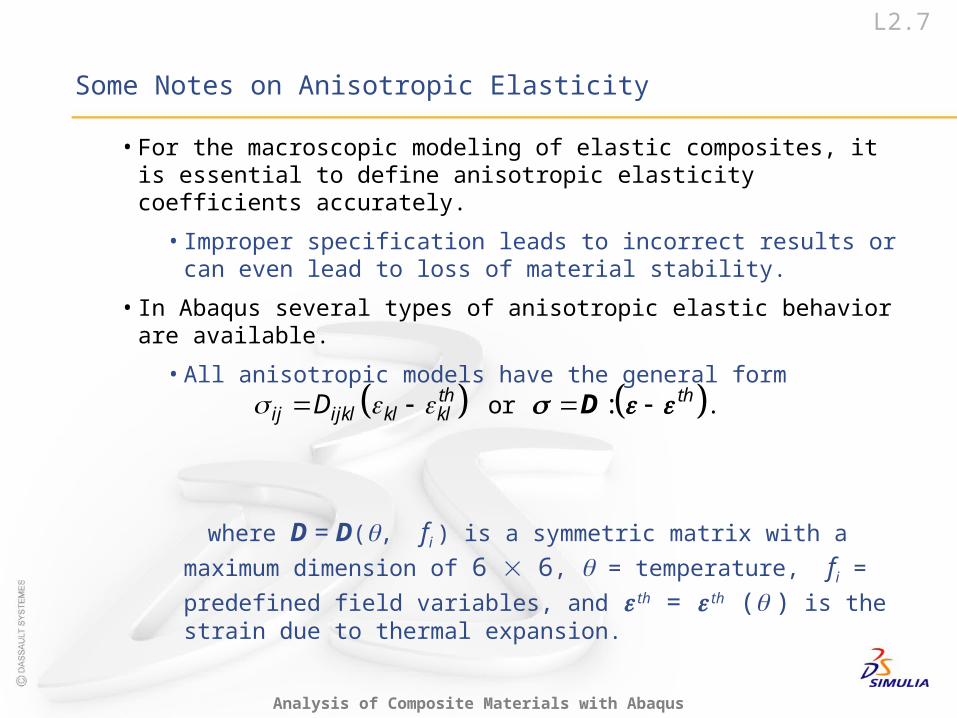
• For the macroscopic modeling of elastic composites, it is essential to define anisotropic elasticity coefficients accurately.
• Improper specification leads to incorrect results or can even lead to loss of material stability.
• In Abaqus several types of anisotropic elastic behavior are available.
• All anisotropic models have the general form
where D = D(, fi ) is a symmetric matrix with a maximum
dimension of 6 6, = temperature, fi = predefined field variables,
and th =
th ( ) is the strain due to thermal expansion.
:th thij ijkl kl klD Dor .
L2.8
Analysis of Composite Materials with Abaqus
Some Notes on Anisotropic Elasticity
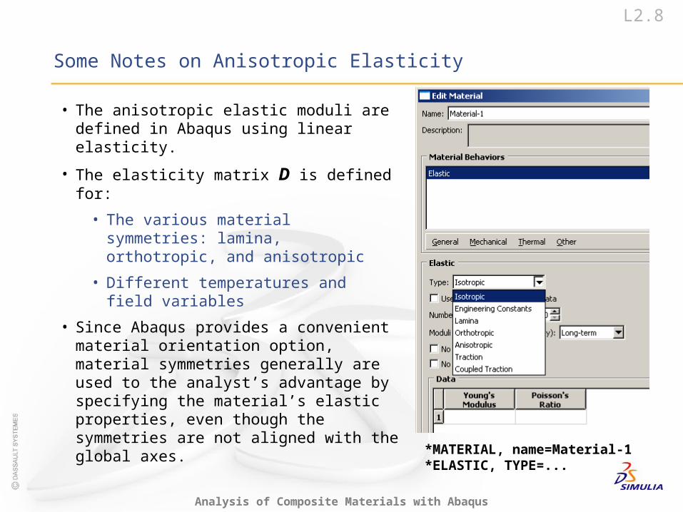
• The anisotropic elastic moduli are defined in Abaqus using linear elasticity.
• The elasticity matrix D is defined for:
• The various material symmetries: lamina, orthotropic, and anisotropic
• Different temperatures and field variables
• Since Abaqus provides a convenient material orientation option, material symmetries generally are used to the analyst’s advantage by specifying the material’s elastic properties, even though the symmetries are not aligned with the global axes.
*MATERIAL, name=Material-1*ELASTIC, TYPE=...
L2.9
Analysis of Composite Materials with Abaqus
Some Notes on Anisotropic Elasticity
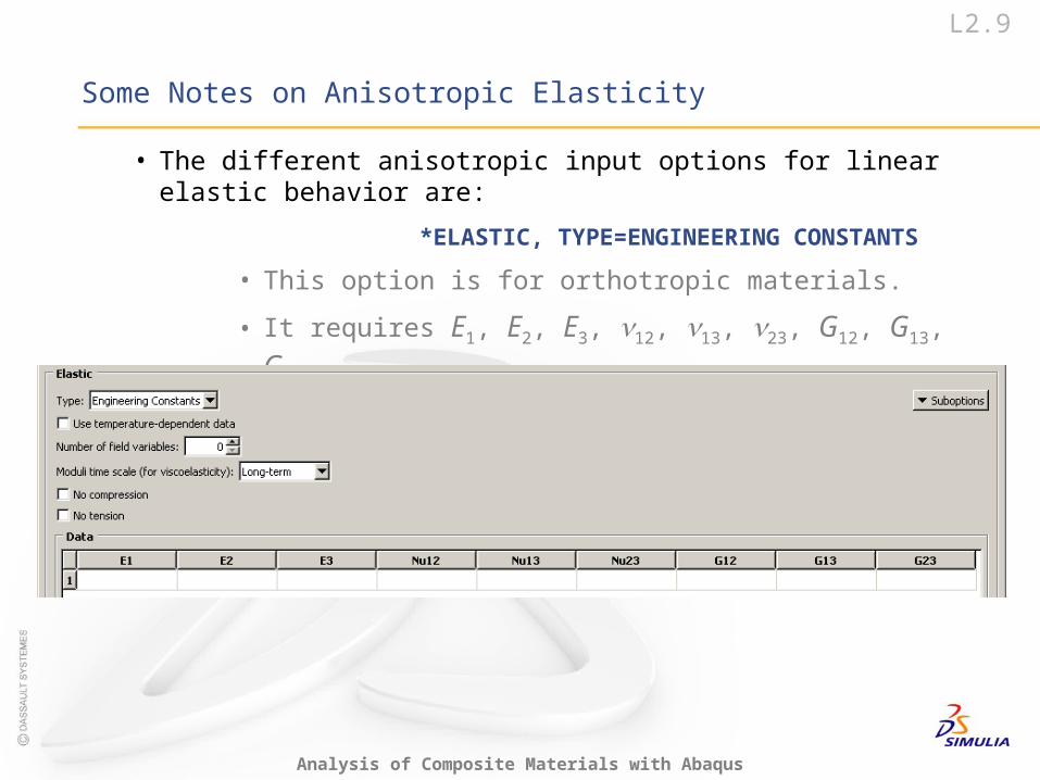
• The different anisotropic input options for linear elastic behavior are:
*ELASTIC, TYPE=ENGINEERING CONSTANTS
• This option is for orthotropic materials.
• It requires E1, E2, E3, 12, 13, 23, G12, G13, G23.
L2.10
Analysis of Composite Materials with Abaqus
Some Notes on Anisotropic Elasticity
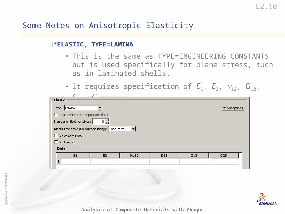
*ELASTIC, TYPE=LAMINA
• This is the same as TYPE=ENGINEERING CONSTANTS but is used specifically for plane stress, such as in laminated shells.
• It requires specification of E1, E2, 12, G12, G13, G23.
L2.11
Analysis of Composite Materials with Abaqus
Some Notes on Anisotropic Elasticity
1111 1122 1133
2222 2233
3333
1212
1313
2323
0 0 0
0 0 0
0 0 0
0 0
sym 0
D D D
D D
D
D
D
D
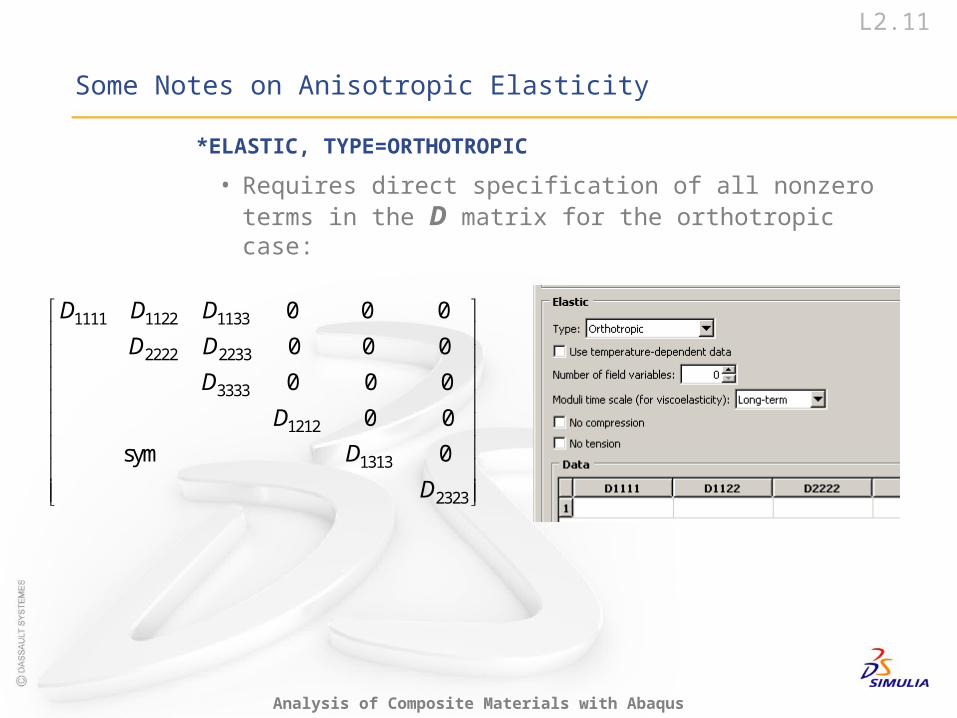
*ELASTIC, TYPE=ORTHOTROPIC
• Requires direct specification of all nonzero terms in the D matrix for the orthotropic case:
L2.12
Analysis of Composite Materials with Abaqus
Some Notes on Anisotropic Elasticity
1111 1122 1133 1112 1113 1123
2222 2233 2212 2213 2223
3333 3312 3313 3323
1212 1213 1223
1313 1323
2323
sym
D D D D D D
D D D D D
D D D D
D D D
D D
D
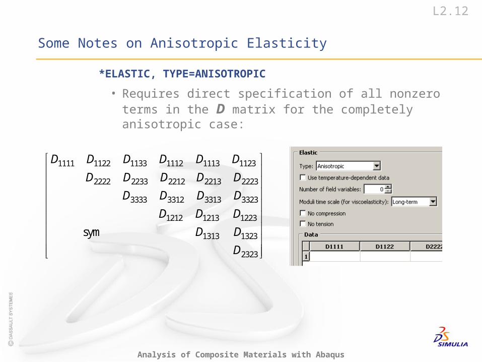
*ELASTIC, TYPE=ANISOTROPIC
• Requires direct specification of all nonzero terms in the D matrix for the completely anisotropic case:
L2.13
Analysis of Composite Materials with Abaqus
Some Notes on Anisotropic Elasticity
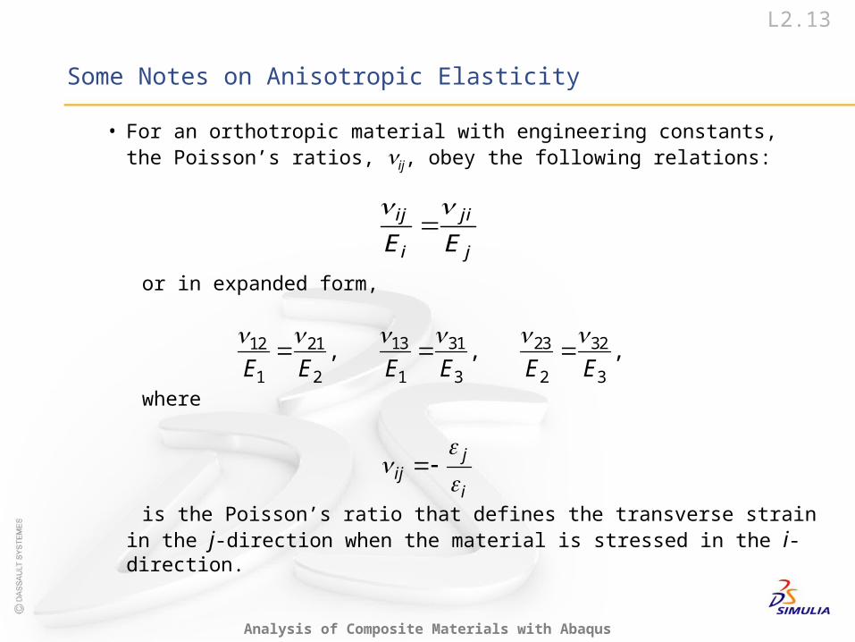
• For an orthotropic material with engineering constants, the Poisson’s ratios, ij, obey the following relations:
or in expanded form,
where
is the Poisson’s ratio that defines the transverse strain in the j-direction when the material is stressed in the i-direction.
ij ji
i jE E
13 31 23 3212 21
1 2 1 3 2 3E E E E E E
, , ,
jij
i

L2.14
Analysis of Composite Materials with Abaqus
Some Notes on Anisotropic Elasticity
• The user should be careful in distinguishing between ij and ji.
• For example, to determine 12 and 21 we do the following two simple
uniaxial tests:

L2.15
Analysis of Composite Materials with Abaqus
Some Notes on Anisotropic Elasticity
• For an orthotropic material the “engineering constants” define the D matrix as:
where
1111 1 23 32
2222 2 13 31
3333 3 12 21
1122 1 21 31 23 2 12 32 13
1133 1 31 21 32 3 13 12 23
2233 2 32 12 31 3 23 21 13
1212 12
1313 13
2323 23
1
1
1
D E
D E
D E
D E E
D E E
D E E
D G
D G
D G
12 21 23 32 31 13 21 32 13
1
1 2
.
L2.16
Analysis of Composite Materials with Abaqus
Some Notes on Anisotropic Elasticity
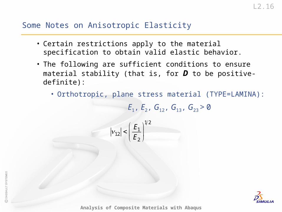
• Certain restrictions apply to the material specification to obtain valid elastic behavior.
• The following are sufficient conditions to ensure material stability (that is, for D to be positive-definite):
• Orthotropic, plane stress material (TYPE=LAMINA):
E1, E2, G12, G13, G23 > 0
1 2
112
2
E
E
L2.17
Analysis of Composite Materials with Abaqus
Some Notes on Anisotropic Elasticity
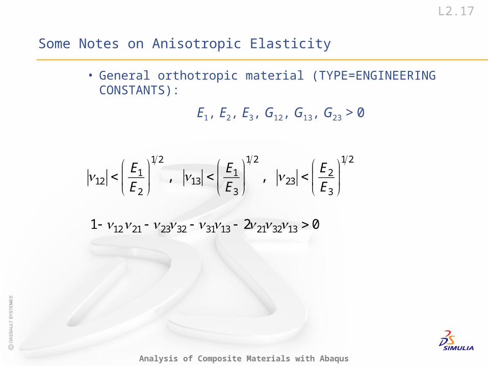
• General orthotropic material (TYPE=ENGINEERING CONSTANTS):
E1, E2, E3, G12, G13, G23 > 0
1 2 1 21 2
1 1 212 13 23
2 3 3
, ,E E E
E E E
12 21 23 32 31 13 21 32 131 2 0
L2.18
Analysis of Composite Materials with Abaqus
Some Notes on Anisotropic Elasticity
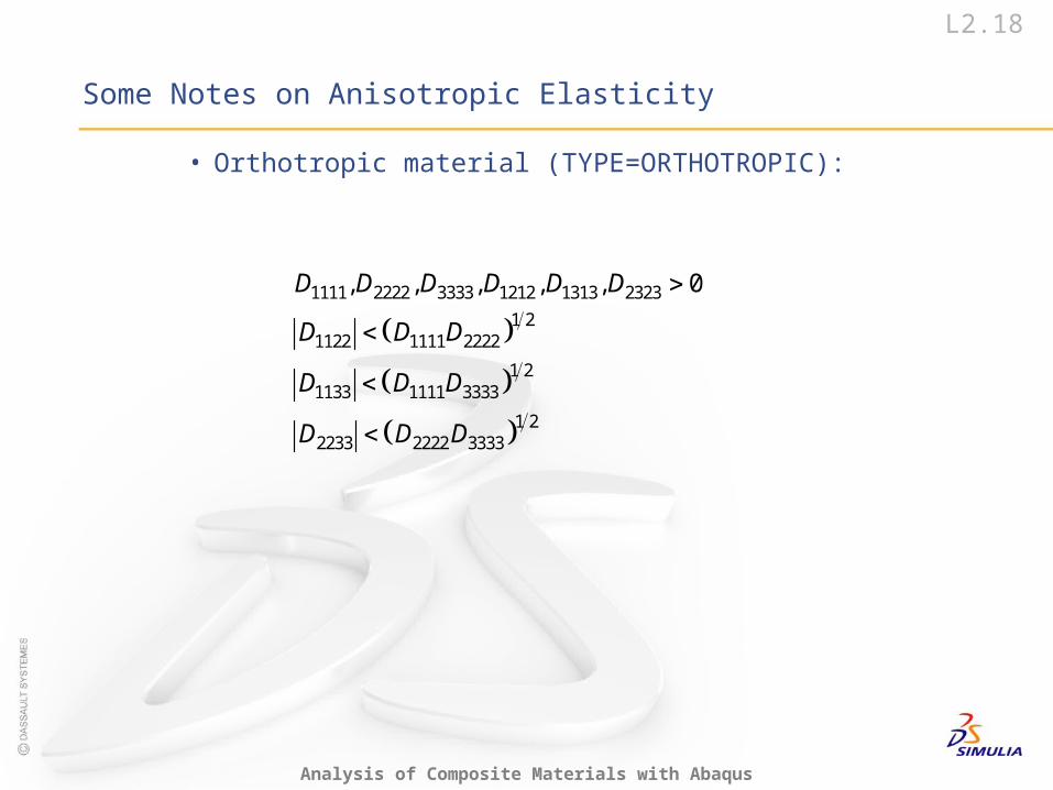
• Orthotropic material (TYPE=ORTHOTROPIC):
1111 2222 3333 1212 1313 2323
1 21122 1111 2222
1 21133 1111 3333
1 22233 2222 3333
0D D D D D D
D D D
D D D
D D D
, , , , ,
L2.19
Analysis of Composite Materials with Abaqus
Some Notes on Anisotropic Elasticity
• Anisotropic material (TYPE=ANISOTROPIC):
• The conditions are too complex to express in simple relations.
• The requirement that D is positive-definite means that all six eigenvalues of D must be positive.
• This should be ascertained numerically before the material description is used in an Abaqus analysis.
Thermal Expansion
L2.21
Analysis of Composite Materials with Abaqus
Thermal Expansion
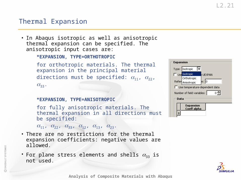
• In Abaqus isotropic as well as anisotropic thermal expansion can be specified. The anisotropic input cases are:
*EXPANSION, TYPE=ORTHOTROPIC
for orthotropic materials. The thermal expansion in the principal material directions must be specified: 11, 22, 33.
*EXPANSION, TYPE=ANISOTROPIC
for fully anisotropic materials. The thermal expansion in all directions must be specified: 11, 22, 33, 12, 13, 23.
• There are no restrictions for the thermal expansion coefficients: negative values are allowed.
• For plane stress elements and shells 33 is not used.
Material Orientation
L2.23
Analysis of Composite Materials with Abaqus
Material Orientation
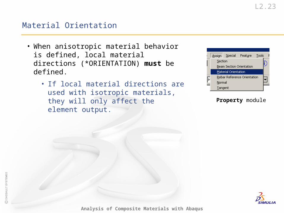
• When anisotropic material behavior is defined, local material directions (*ORIENTATION) must be defined.
• If local material directions are used with isotropic materials, they will only affect the element output.
Property module
L2.24
Analysis of Composite Materials with Abaqus
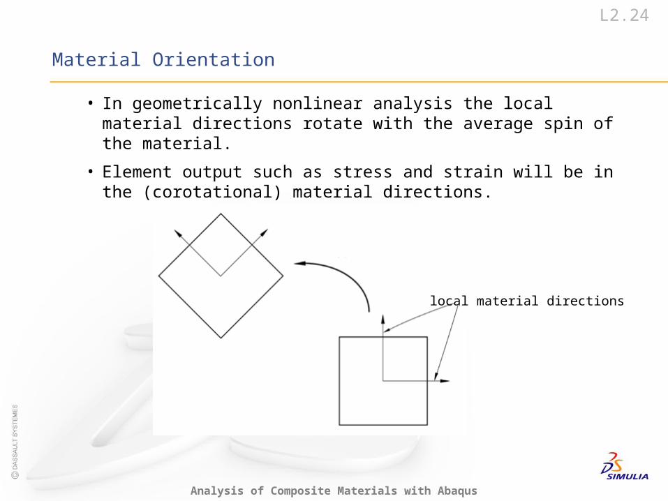
Material Orientation
• In geometrically nonlinear analysis the local material directions rotate with the average spin of the material.
• Element output such as stress and strain will be in the (corotational) material directions.
local material directions
L2.25
Analysis of Composite Materials with Abaqus
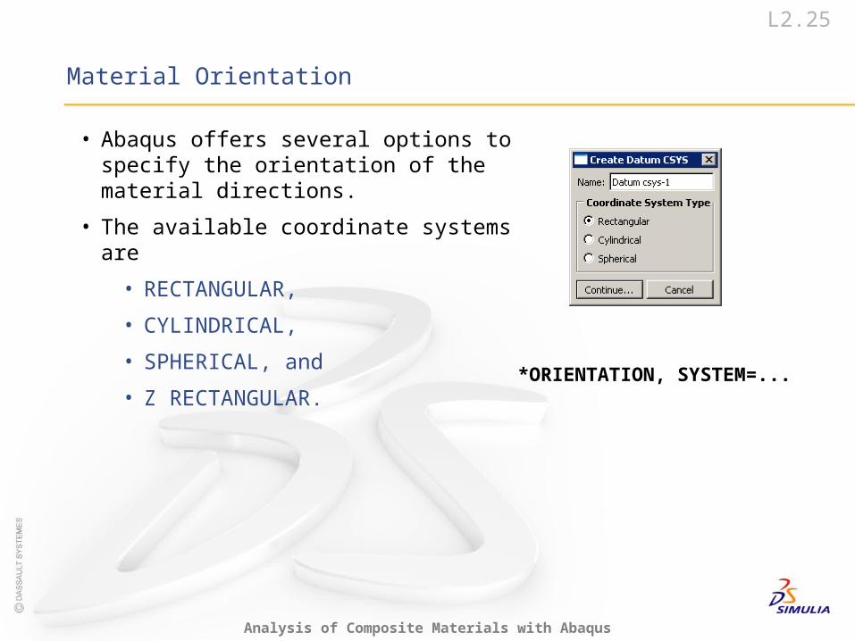
Material Orientation
• Abaqus offers several options to specify the orientation of the material directions.
• The available coordinate systems are
• RECTANGULAR,
• CYLINDRICAL,
• SPHERICAL, and
• Z RECTANGULAR.*ORIENTATION, SYSTEM=...
L2.26
Analysis of Composite Materials with Abaqus
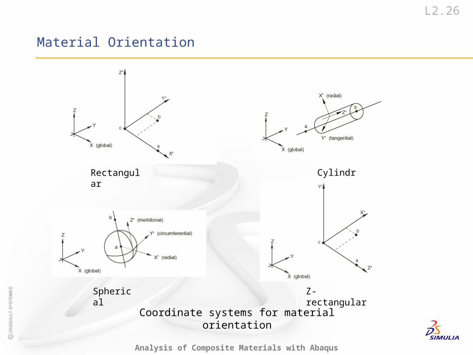
Material Orientation
Coordinate systems for material orientation
Rectangular
Spherical
Cylindrical
Z-rectangular
L2.27
Analysis of Composite Materials with Abaqus
Material Orientation
• Additional comments on the keywords interface
• The orientation and position of the local coordinate system is defined by the coordinates of two points, a and b.
• The DEFINITION parameter specifies how the coordinates of these points are defined.
• The options are NODES, COORDINATES, and OFFSET TO NODES.
• If no further data are given, the principal axes of the material will be aligned with the local coordinate system.
• Optionally, the principal axes of the material can be rotated around one of the local coordinate directions.
• If the orientation is too complex to be specified with these options, user subroutine ORIENT can be invoked with the parameter SYSTEM=USER.

L2.28
Analysis of Composite Materials with Abaqus
Material Orientation
• Example: Cylindrical orientation
• Abaqus/CAE interface
1
2b
define a cylindrical coordinate system
2aselect regions and the datum coordinate system
43
RZ
T
n1
2
n1
2
12
n
1 2
n
12n
12
n
L2.29
Analysis of Composite Materials with Abaqus
Material Orientation
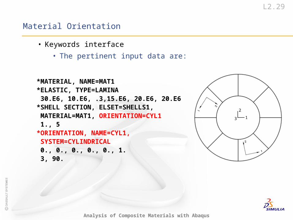
• Keywords interface
• The pertinent input data are:
*MATERIAL, NAME=MAT1*ELASTIC, TYPE=LAMINA 30.E6, 10.E6, .3,15.E6, 20.E6, 20.E6*SHELL SECTION, ELSET=SHELLS1, MATERIAL=MAT1, ORIENTATION=CYL1 1., 5*ORIENTATION, NAME=CYL1, SYSTEM=CYLINDRICAL 0., 0., 0., 0., 0., 1. 3, 90.
1
2
3

Almost Incompressible Behavior
L2.31
Analysis of Composite Materials with Abaqus
Almost Incompressible Behavior
• For certain types of composites the elastic bulk modulus, K, is much larger than the effective elastic shear modulus, Geff : the material is
essentially incompressible.
• We should check this since, except for plane stress cases, almost incompressible behavior requires the use of special element formulations.
• First, we need values for K and Geff , or we can estimate the effective
Poisson’s ratio.
L2.32
Analysis of Composite Materials with Abaqus
Almost Incompressible Behavior
• For a general, anisotropic, linear elastic stress-strain law we can compute the bulk modulus from its definition:
where the equivalent pressure stress, p, is
and the elastic strain, , is decomposed into its volumetric and deviatoric parts:
where vol is a scalar quantity.
volK p ,
def 1 1: : :
3 3p I I D
1
3 vol dev I ,
L2.33
Analysis of Composite Materials with Abaqus
• Therefore,
and since the bulk modulus is
• For example, for TYPE=ENGINEERING CONSTANTS
• A conservative (low) estimate of the effective elastic shear modulus can be obtained by taking the minimum of G12, G13, and G23.
1/ : : /
3vol volK p I D ,
1: :
9K I D I.
12 13 21 23 31 32
1 2 3
1
1 1 1K
E E E
.
1/
3vol I,
Almost Incompressible Behavior
L2.34
Analysis of Composite Materials with Abaqus
Almost Incompressible Behavior
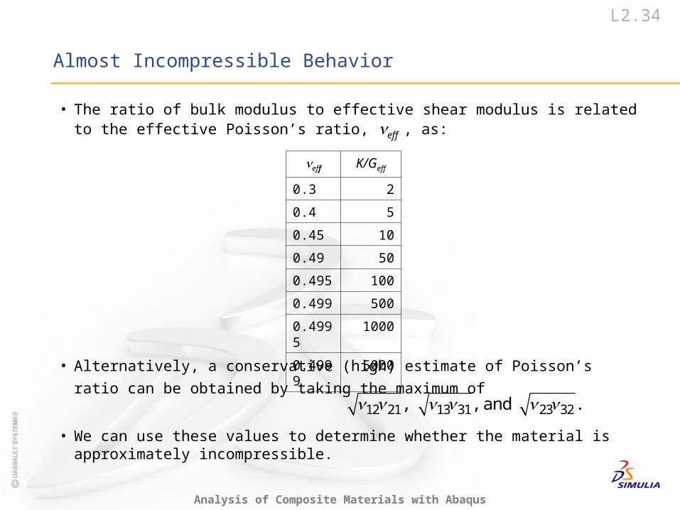
• The ratio of bulk modulus to effective shear modulus is related to the effective Poisson’s ratio, eff , as:
• Alternatively, a conservative (high) estimate of Poisson’s ratio can be
obtained by taking the maximum of
• We can use these values to determine whether the material is approximately incompressible.
eff K/Geff
0.3 2
0.4 5
0.45 10
0.49 50
0.495 100
0.499 500
0.4995 1000
0.4999 5000
12 21 13 31 23 32 , , and .

L2.35
Analysis of Composite Materials with Abaqus
Almost Incompressible Behavior
• If K/Geff > 100 or eff > 0.495, the stiffness ratio between volumetric and
shear deformation is too high to use standard displacement formulation elements: mesh locking is likely to occur.
• Reduced integration elements can be used to avoid locking effects.
• Abaqus uses selectively reduced integration for the standard lower-order quadrilateral and brick elements (CPE4, CAX4, C3D8, etc.), which also prevents locking.
• The alternative is to use “hybrid” (mixed formulation) elements (element types CxxH, such as C3D20H).
• Use of hybrid elements is necessary if the material is essentially incompressible (K ).
• For any plane stress application (beams, shells, and continuum plane stress elements), standard displacement elements can always be used for any value of eff .