COMP 790.139 (Fall 2017) Natural Language...
67
COMP 790.139 (Fall 2017) Natural Language Processing (with deep learning and connections to vision/robotics) Mohit Bansal (various slides adapted/borrowed from courses by Dan Klein, Richard Socher, Chris Manning, others)
Transcript of COMP 790.139 (Fall 2017) Natural Language...

COMP 790.139 (Fall 2017) Natural Language Processing
(with deep learning and connections to vision/robotics)
Mohit Bansal
(various slides adapted/borrowed from courses by Dan Klein, Richard Socher, Chris Manning, others)

Announcements
! Chapter section summaries were due yesterday
! Make sure you regularly check your ConnectCarolina email id’s
! 1st Coding assignment to be out soon
! Start thinking of projects early!
! TA: Yixin Nie ([email protected]) -- will announce office hours
soon!

Recap of Distributional Semantics
! Words occurring in similar context have similar linguistic behavior (meaning) [Harris, 1954; Firth, 1957]
! Traditional approach: context-counting vectors ! Count left and right context in window ! Reweight with PMI or LLR ! Reduce dimensionality with SVD or NNMF
[Pereira et al., 1993; Lund & Burgess, 1996; Lin, 1998; Lin and Pantel, 2001; Sahlgren, 2006; Pado & Lapata, 2007; Turney and Pantel, 2010; Baroni and Lenci, 2010]
! More word representations: hierarchical clustering based on
bigram LM LL [Brown et al., 1992]
Ms. Haag plays Elianti .*
objproot
nmod sbj
Figure 1: An example of a labeled dependency tree. Thetree contains a special token “*” which is always the rootof the tree. Each arc is directed from head to modifier andhas a label describing the function of the attachment.
and clustering, Section 3 describes the cluster-basedfeatures, Section 4 presents our experimental results,Section 5 discusses related work, and Section 6 con-cludes with ideas for future research.
2 Background
2.1 Dependency parsing
Recent work (Buchholz and Marsi, 2006; Nivreet al., 2007) has focused on dependency parsing.Dependency syntax represents syntactic informa-tion as a network of head-modifier dependency arcs,typically restricted to be a directed tree (see Fig-ure 1 for an example). Dependency parsing dependscritically on predicting head-modifier relationships,which can be difficult due to the statistical sparsityof these word-to-word interactions. Bilexical depen-dencies are thus ideal candidates for the applicationof coarse word proxies such as word clusters.
In this paper, we take a part-factored structuredclassification approach to dependency parsing. For agiven sentence x, let Y(x) denote the set of possibledependency structures spanning x, where each y �Y(x) decomposes into a set of “parts” r � y. In thesimplest case, these parts are the dependency arcsthemselves, yielding a first-order or “edge-factored”dependency parsing model. In higher-order parsingmodels, the parts can consist of interactions betweenmore than two words. For example, the parser ofMcDonald and Pereira (2006) defines parts for sib-ling interactions, such as the trio “plays”, “Elianti”,and “.” in Figure 1. The Carreras (2007) parserhas parts for both sibling interactions and grandpar-ent interactions, such as the trio “*”, “plays”, and“Haag” in Figure 1. These kinds of higher-orderfactorizations allow dependency parsers to obtain alimited form of context-sensitivity.
Given a factorization of dependency structuresinto parts, we restate dependency parsing as the fol-
apple pear Apple IBM bought run of in
01
100 101 110 111000 001 010 011
00
0
10
1
11
Figure 2: An example of a Brown word-cluster hierarchy.Each node in the tree is labeled with a bit-string indicat-ing the path from the root node to that node, where 0indicates a left branch and 1 indicates a right branch.
lowing maximization:
PARSE(x;w) = argmaxy�Y(x)
X
r�y
w · f(x, r)
Above, we have assumed that each part is scoredby a linear model with parameters w and feature-mapping f(·). For many different part factoriza-tions and structure domains Y(·), it is possible tosolve the above maximization efficiently, and severalrecent efforts have concentrated on designing newmaximization algorithms with increased context-sensitivity (Eisner, 2000; McDonald et al., 2005b;McDonald and Pereira, 2006; Carreras, 2007).
2.2 Brown clustering algorithmIn order to provide word clusters for our exper-iments, we used the Brown clustering algorithm(Brown et al., 1992). We chose to work with theBrown algorithm due to its simplicity and prior suc-cess in other NLP applications (Miller et al., 2004;Liang, 2005). However, we expect that our approachcan function with other clustering algorithms (as in,e.g., Li and McCallum (2005)). We briefly describethe Brown algorithm below.
The input to the algorithm is a vocabulary ofwords to be clustered and a corpus of text containingthese words. Initially, each word in the vocabularyis considered to be in its own distinct cluster. The al-gorithm then repeatedly merges the pair of clusterswhich causes the smallest decrease in the likelihoodof the text corpus, according to a class-based bigramlanguage model defined on the word clusters. Bytracing the pairwise merge operations, one obtainsa hierarchical clustering of the words, which can berepresented as a binary tree as in Figure 2.
Within this tree, each word is uniquely identifiedby its path from the root, and this path can be com-pactly represented with a bit string, as in Figure 2.In order to obtain a clustering of the words, we se-lect all nodes at a certain depth from the root of the
food
0.6 -0.2 0.9 0.3 -0.4 0.5
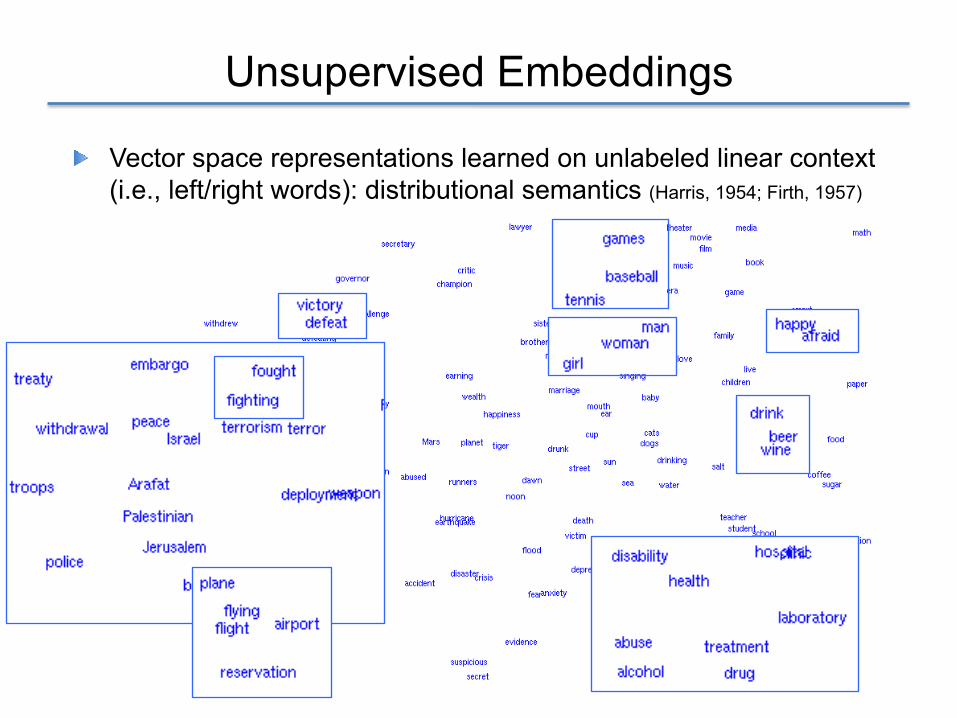
Unsupervised Embeddings
! Vector space representations learned on unlabeled linear context (i.e., left/right words): distributional semantics (Harris, 1954; Firth, 1957)
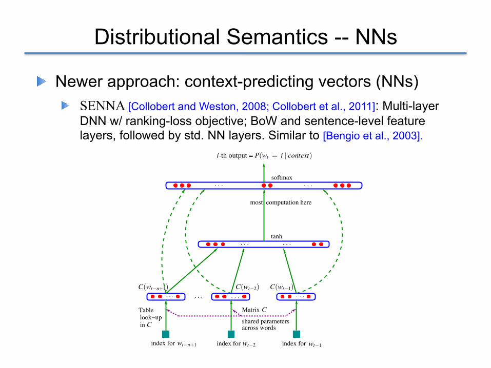
Distributional Semantics -- NNs
! Newer approach: context-predicting vectors (NNs) ! SENNA [Collobert and Weston, 2008; Collobert et al., 2011]: Multi-layer
DNN w/ ranking-loss objective; BoW and sentence-level feature layers, followed by std. NN layers. Similar to [Bengio et al., 2003].
BENGIO, DUCHARME, VINCENT AND JAUVIN
softmax
tanh
. . . . . .. . .
. . . . . .
. . . . . .
across words
most computation here
index for index for index for
shared parameters
Matrix
inlook−upTable
. . .
C
C
wt�1wt�2
C(wt�2) C(wt�1)C(wt�n+1)
wt�n+1
i-th output = P(wt = i | context)
Figure 1: Neural architecture: f (i,wt�1, · · · ,wt�n+1) = g(i,C(wt�1), · · · ,C(wt�n+1)) where g is theneural network andC(i) is the i-th word feature vector.
parameters of the mapping C are simply the feature vectors themselves, represented by a |V |⇥mmatrixC whose row i is the feature vectorC(i) for word i. The function g may be implemented by afeed-forward or recurrent neural network or another parametrized function, with parameters ω. Theoverall parameter set is θ= (C,ω).
Training is achieved by looking for θ that maximizes the training corpus penalized log-likelihood:
L=1T ∑t
log f (wt ,wt�1, · · · ,wt�n+1;θ)+R(θ),
where R(θ) is a regularization term. For example, in our experiments, R is a weight decay penaltyapplied only to the weights of the neural network and to theC matrix, not to the biases.3
In the above model, the number of free parameters only scales linearly with V , the number ofwords in the vocabulary. It also only scales linearly with the order n : the scaling factor couldbe reduced to sub-linear if more sharing structure were introduced, e.g. using a time-delay neuralnetwork or a recurrent neural network (or a combination of both).
In most experiments below, the neural network has one hidden layer beyond the word featuresmapping, and optionally, direct connections from the word features to the output. Therefore thereare really two hidden layers: the shared word features layer C, which has no non-linearity (it wouldnot add anything useful), and the ordinary hyperbolic tangent hidden layer. More precisely, theneural network computes the following function, with a softmax output layer, which guaranteespositive probabilities summing to 1:
P(wt |wt�1, · · ·wt�n+1) =eywt∑i eyi
.
3. The biases are the additive parameters of the neural network, such as b and d in equation 1 below.
1142

Distributional Semantics -- NNs
! CBOW, SKIP, word2vec [Mikolov et al., 2013]: Simple, super-fast NN w/ no hidden layer. Continuous BoW model predicts word given context, skip-gram model predicts surrounding context words given current word
! Other: [Mnih and Hinton, 2007; Turian et al., 2010]
! Demos: h#ps://code.google.com/p/word2vec,h#p://metaop7mize.com/projects/wordreprs/, h#p://ml.nec-labs.com/senna/
w(t-2)
w(t+1)
w(t-1)
w(t+2)
w(t)
SUM
INPUT PROJECTION OUTPUT
w(t)
INPUT PROJECTION OUTPUT
w(t-2)
w(t-1)
w(t+1)
w(t+2)
CBOW Skip-gram
Figure 1: New model architectures. The CBOW architecture predicts the current word based on thecontext, and the Skip-gram predicts surrounding words given the current word.
R words from the future of the current word as correct labels. This will require us to do R ⇥ 2word classifications, with the current word as input, and each of the R + R words as output. In thefollowing experiments, we use C = 10.
4 Results
To compare the quality of different versions of word vectors, previous papers typically use a tableshowing example words and their most similar words, and understand them intuitively. Althoughit is easy to show that word France is similar to Italy and perhaps some other countries, it is muchmore challenging when subjecting those vectors in a more complex similarity task, as follows. Wefollow previous observation that there can be many different types of similarities between words, forexample, word big is similar to bigger in the same sense that small is similar to smaller. Exampleof another type of relationship can be word pairs big - biggest and small - smallest [20]. We furtherdenote two pairs of words with the same relationship as a question, as we can ask: ”What is theword that is similar to small in the same sense as biggest is similar to big?”
Somewhat surprisingly, these questions can be answered by performing simple algebraic operationswith the vector representation of words. To find a word that is similar to small in the same sense asbiggest is similar to big, we can simply compute vector X = vector(”biggest”)�vector(”big”)+vector(”small”). Then, we search in the vector space for the word closest to X measured by cosinedistance, and use it as the answer to the question (we discard the input question words during thissearch). When the word vectors are well trained, it is possible to find the correct answer (wordsmallest) using this method.
Finally, we found that when we train high dimensional word vectors on a large amount of data, theresulting vectors can be used to answer very subtle semantic relationships between words, such asa city and the country it belongs to, e.g. France is to Paris as Germany is to Berlin. Word vectorswith such semantic relationships could be used to improve many existing NLP applications, suchas machine translation, information retrieval and question answering systems, and may enable otherfuture applications yet to be invented.
5

Skipgram word2vec [Mikolov et al., 2013]
Few mins. vs. days/weeks/months!!
w(t)
w(t-2)
w(t-1)
w(t+1)
w(t+2)
INPUT PROJECTION OUTPUT
context window
w

Skip-gram word2vec Objective Function
! Objective of Skip-gram model is to max. the avg. log probability:
!"#$
%&'(#)))))))))))'*+,-.#/+&))))))+(#'(#
!"#01$
!"#02$
!"#32$
!"#31$
Figure 1: The Skip-gram model architecture. The training objective is to learn word vector representationsthat are good at predicting the nearby words.
In this paper we present several extensions of the original Skip-gram model. We show that sub-sampling of frequent words during training results in a significant speedup (around 2x - 10x), andimproves accuracy of the representations of less frequent words. In addition, we present a simpli-fied variant of Noise Contrastive Estimation (NCE) [4] for training the Skip-grammodel that resultsin faster training and better vector representations for frequent words, compared to more complexhierarchical softmax that was used in the prior work [8].
Word representations are limited by their inability to represent idiomatic phrases that are not com-positions of the individual words. For example, “Boston Globe” is a newspaper, and so it is not anatural combination of the meanings of “Boston” and “Globe”. Therefore, using vectors to repre-sent the whole phrases makes the Skip-gram model considerably more expressive. Other techniquesthat aim to represent meaning of sentences by composing the word vectors, such as the recursiveautoencoders [15], would also benefit from using phrase vectors instead of the word vectors.
The extension from word based to phrase based models is relatively simple. First we identify a largenumber of phrases using a data-driven approach, and then we treat the phrases as individual tokensduring the training. To evaluate the quality of the phrase vectors, we developed a test set of analogi-cal reasoning tasks that contains both words and phrases. A typical analogy pair from our test set is“Montreal”:“Montreal Canadiens”::“Toronto”:“TorontoMaple Leafs”. It is considered to have beenanswered correctly if the nearest representation to vec(“Montreal Canadiens”) - vec(“Montreal”) +vec(“Toronto”) is vec(“Toronto Maple Leafs”).
Finally, we describe another interesting property of the Skip-gram model. We found that simplevector addition can often produce meaningful results. For example, vec(“Russia”) + vec(“river”) isclose to vec(“Volga River”), and vec(“Germany”) + vec(“capital”) is close to vec(“Berlin”). Thiscompositionality suggests that a non-obvious degree of language understanding can be obtained byusing basic mathematical operations on the word vector representations.
2 The Skip-gram Model
The training objective of the Skip-gram model is to find word representations that are useful forpredicting the surrounding words in a sentence or a document. More formally, given a sequence oftraining wordsw1, w2, w3, . . . , wT , the objective of the Skip-grammodel is to maximize the averagelog probability
1
T
T!
t=1
!
−c≤j≤c,j =0
log p(wt+j |wt) (1)
where c is the size of the training context (which can be a function of the center word wt). Largerc results in more training examples and thus can lead to a higher accuracy, at the expense of the
2
training time. The basic Skip-gram formulation defines p(wt+j |wt) using the softmax function:
p(wO|wI) =exp
!
v′wO
⊤vwI
"
#Ww=1 exp
!
v′w⊤vwI
" (2)
where vw and v′w are the “input” and “output” vector representations of w, and W is the num-ber of words in the vocabulary. This formulation is impractical because the cost of computing∇ log p(wO|wI) is proportional toW , which is often large (105–107 terms).
2.1 Hierarchical Softmax
A computationally efficient approximation of the full softmax is the hierarchical softmax. In thecontext of neural network language models, it was first introduced by Morin and Bengio [12]. Themain advantage is that instead of evaluating W output nodes in the neural network to obtain theprobability distribution, it is needed to evaluate only about log2(W ) nodes.
The hierarchical softmax uses a binary tree representation of the output layer with theW words asits leaves and, for each node, explicitly represents the relative probabilities of its child nodes. Thesedefine a random walk that assigns probabilities to words.
More precisely, each word w can be reached by an appropriate path from the root of the tree. Letn(w, j) be the j-th node on the path from the root to w, and let L(w) be the length of this path, son(w, 1) = root and n(w,L(w)) = w. In addition, for any inner node n, let ch(n) be an arbitraryfixed child of n and let [[x]] be 1 if x is true and -1 otherwise. Then the hierarchical softmax definesp(wO|wI) as follows:
p(w|wI ) =
L(w)−1$
j=1
σ!
[[n(w, j + 1) = ch(n(w, j))]] · v′n(w,j)⊤vwI
"
(3)
where σ(x) = 1/(1 + exp(−x)). It can be verified that#W
w=1 p(w|wI) = 1. This implies that thecost of computing log p(wO|wI) and ∇ log p(wO|wI) is proportional to L(wO), which on averageis no greater than logW . Also, unlike the standard softmax formulation of the Skip-gram whichassigns two representations vw and v′w to each word w, the hierarchical softmax formulation hasone representation vw for each word w and one representation v′n for every inner node n of thebinary tree.
The structure of the tree used by the hierarchical softmax has a considerable effect on the perfor-mance. Mnih and Hinton explored a number of methods for constructing the tree structure and theeffect on both the training time and the resulting model accuracy [10]. In our work we use a binaryHuffman tree, as it assigns short codes to the frequent words which results in fast training. It hasbeen observed before that grouping words together by their frequency works well as a very simplespeedup technique for the neural network based language models [5, 8].
2.2 Negative Sampling
An alternative to the hierarchical softmax is Noise Contrastive Estimation (NCE), which was in-troduced by Gutmann and Hyvarinen [4] and applied to language modeling by Mnih and Teh [11].NCE posits that a good model should be able to differentiate data from noise by means of logisticregression. This is similar to hinge loss used by Collobert and Weston [2] who trained the modelsby ranking the data above noise.
While NCE can be shown to approximately maximize the log probability of the softmax, the Skip-gram model is only concerned with learning high-quality vector representations, so we are free tosimplify NCE as long as the vector representations retain their quality. We define Negative sampling(NEG) by the objective
log σ(v′wO
⊤vwI
) +k%
i=1
Ewi∼Pn(w)
&
log σ(−v′wi
⊤vwI
)'
(4)
3
! The above conditional probability is defined via the softmax function:
where v and v′ are the “input” and “output” vector representations of w, and W is the number of words in the vocabulary
[Mikolov et al., 2013]

Efficient Skip-gram word2vec:
! Negative Sampling:
! I.e., to distinguish the target word wo from draws from the noise distribution Pn(w) using logistic regression, where there are k negative samples for each data sample.
training time. The basic Skip-gram formulation defines p(wt+j |wt) using the softmax function:
p(wO|wI) =exp
!
v′wO
⊤vwI
"
#Ww=1 exp
!
v′w⊤vwI
" (2)
where vw and v′w are the “input” and “output” vector representations of w, and W is the num-ber of words in the vocabulary. This formulation is impractical because the cost of computing∇ log p(wO|wI) is proportional toW , which is often large (105–107 terms).
2.1 Hierarchical Softmax
A computationally efficient approximation of the full softmax is the hierarchical softmax. In thecontext of neural network language models, it was first introduced by Morin and Bengio [12]. Themain advantage is that instead of evaluating W output nodes in the neural network to obtain theprobability distribution, it is needed to evaluate only about log2(W ) nodes.
The hierarchical softmax uses a binary tree representation of the output layer with theW words asits leaves and, for each node, explicitly represents the relative probabilities of its child nodes. Thesedefine a random walk that assigns probabilities to words.
More precisely, each word w can be reached by an appropriate path from the root of the tree. Letn(w, j) be the j-th node on the path from the root to w, and let L(w) be the length of this path, son(w, 1) = root and n(w,L(w)) = w. In addition, for any inner node n, let ch(n) be an arbitraryfixed child of n and let [[x]] be 1 if x is true and -1 otherwise. Then the hierarchical softmax definesp(wO|wI) as follows:
p(w|wI ) =
L(w)−1$
j=1
σ!
[[n(w, j + 1) = ch(n(w, j))]] · v′n(w,j)⊤vwI
"
(3)
where σ(x) = 1/(1 + exp(−x)). It can be verified that#W
w=1 p(w|wI) = 1. This implies that thecost of computing log p(wO|wI) and ∇ log p(wO|wI) is proportional to L(wO), which on averageis no greater than logW . Also, unlike the standard softmax formulation of the Skip-gram whichassigns two representations vw and v′w to each word w, the hierarchical softmax formulation hasone representation vw for each word w and one representation v′n for every inner node n of thebinary tree.
The structure of the tree used by the hierarchical softmax has a considerable effect on the perfor-mance. Mnih and Hinton explored a number of methods for constructing the tree structure and theeffect on both the training time and the resulting model accuracy [10]. In our work we use a binaryHuffman tree, as it assigns short codes to the frequent words which results in fast training. It hasbeen observed before that grouping words together by their frequency works well as a very simplespeedup technique for the neural network based language models [5, 8].
2.2 Negative Sampling
An alternative to the hierarchical softmax is Noise Contrastive Estimation (NCE), which was in-troduced by Gutmann and Hyvarinen [4] and applied to language modeling by Mnih and Teh [11].NCE posits that a good model should be able to differentiate data from noise by means of logisticregression. This is similar to hinge loss used by Collobert and Weston [2] who trained the modelsby ranking the data above noise.
While NCE can be shown to approximately maximize the log probability of the softmax, the Skip-gram model is only concerned with learning high-quality vector representations, so we are free tosimplify NCE as long as the vector representations retain their quality. We define Negative sampling(NEG) by the objective
log σ(v′wO
⊤vwI
) +k%
i=1
Ewi∼Pn(w)
&
log σ(−v′wi
⊤vwI
)'
(4)
3
[Mikolov et al., 2013]
Efficient Skip-gram word2vec:
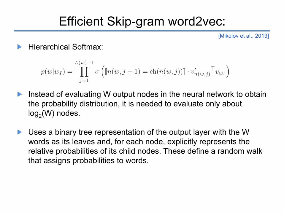
! Hierarchical Softmax:
! Instead of evaluating W output nodes in the neural network to obtain the probability distribution, it is needed to evaluate only about log2(W) nodes.
! Uses a binary tree representation of the output layer with the W words as its leaves and, for each node, explicitly represents the relative probabilities of its child nodes. These define a random walk that assigns probabilities to words.
training time. The basic Skip-gram formulation defines p(wt+j |wt) using the softmax function:
p(wO|wI) =exp
!
v′wO
⊤vwI
"
#Ww=1 exp
!
v′w⊤vwI
" (2)
where vw and v′w are the “input” and “output” vector representations of w, and W is the num-ber of words in the vocabulary. This formulation is impractical because the cost of computing∇ log p(wO|wI) is proportional toW , which is often large (105–107 terms).
2.1 Hierarchical Softmax
A computationally efficient approximation of the full softmax is the hierarchical softmax. In thecontext of neural network language models, it was first introduced by Morin and Bengio [12]. Themain advantage is that instead of evaluating W output nodes in the neural network to obtain theprobability distribution, it is needed to evaluate only about log2(W ) nodes.
The hierarchical softmax uses a binary tree representation of the output layer with theW words asits leaves and, for each node, explicitly represents the relative probabilities of its child nodes. Thesedefine a random walk that assigns probabilities to words.
More precisely, each word w can be reached by an appropriate path from the root of the tree. Letn(w, j) be the j-th node on the path from the root to w, and let L(w) be the length of this path, son(w, 1) = root and n(w,L(w)) = w. In addition, for any inner node n, let ch(n) be an arbitraryfixed child of n and let [[x]] be 1 if x is true and -1 otherwise. Then the hierarchical softmax definesp(wO|wI) as follows:
p(w|wI ) =
L(w)−1$
j=1
σ!
[[n(w, j + 1) = ch(n(w, j))]] · v′n(w,j)⊤vwI
"
(3)
where σ(x) = 1/(1 + exp(−x)). It can be verified that#W
w=1 p(w|wI) = 1. This implies that thecost of computing log p(wO|wI) and ∇ log p(wO|wI) is proportional to L(wO), which on averageis no greater than logW . Also, unlike the standard softmax formulation of the Skip-gram whichassigns two representations vw and v′w to each word w, the hierarchical softmax formulation hasone representation vw for each word w and one representation v′n for every inner node n of thebinary tree.
The structure of the tree used by the hierarchical softmax has a considerable effect on the perfor-mance. Mnih and Hinton explored a number of methods for constructing the tree structure and theeffect on both the training time and the resulting model accuracy [10]. In our work we use a binaryHuffman tree, as it assigns short codes to the frequent words which results in fast training. It hasbeen observed before that grouping words together by their frequency works well as a very simplespeedup technique for the neural network based language models [5, 8].
2.2 Negative Sampling
An alternative to the hierarchical softmax is Noise Contrastive Estimation (NCE), which was in-troduced by Gutmann and Hyvarinen [4] and applied to language modeling by Mnih and Teh [11].NCE posits that a good model should be able to differentiate data from noise by means of logisticregression. This is similar to hinge loss used by Collobert and Weston [2] who trained the modelsby ranking the data above noise.
While NCE can be shown to approximately maximize the log probability of the softmax, the Skip-gram model is only concerned with learning high-quality vector representations, so we are free tosimplify NCE as long as the vector representations retain their quality. We define Negative sampling(NEG) by the objective
log σ(v′wO
⊤vwI
) +k%
i=1
Ewi∼Pn(w)
&
log σ(−v′wi
⊤vwI
)'
(4)
3
[Mikolov et al., 2013]

Analogy Properties Learned [Mikolov et al., 2013]
Figure 2: Left panel shows vector offsets for three wordpairs illustrating the gender relation. Right panel showsa different projection, and the singular/plural relation fortwo words. In high-dimensional space, multiple relationscan be embedded for a single word.
provided. We have explored several related meth-ods and found that the proposed method performswell for both syntactic and semantic relations. Wenote that this measure is qualitatively similar to rela-tional similarity model of (Turney, 2012), which pre-dicts similarity between members of the word pairs(xb, xd), (xc, xd) and dis-similarity for (xa, xd).
6 Experimental Results
To evaluate the vector offset method, we usedvectors generated by the RNN toolkit of Mikolov(2012). Vectors of dimensionality 80, 320, and 640were generated, along with a composite of severalsystems, with total dimensionality 1600. The sys-tems were trained with 320M words of BroadcastNews data as described in (Mikolov et al., 2011a),and had an 82k vocabulary. Table 2 shows resultsfor both RNNLM and LSA vectors on the syntactictask. LSA was trained on the same data as the RNN.We see that the RNN vectors capture significantlymore syntactic regularity than the LSA vectors, anddo remarkably well in an absolute sense, answeringmore than one in three questions correctly. 2
In Table 3 we compare the RNN vectors withthose based on the methods of Collobert and We-ston (2008) and Mnih and Hinton (2009), as imple-mented by (Turian et al., 2010) and available online3 Since different words are present in these datasets,we computed the intersection of the vocabularies ofthe RNN vectors and the new vectors, and restrictedthe test set and word vectors to those. This resultedin a 36k word vocabulary, and a test set with 6632
2Guessing gets a small fraction of a percent.3http://metaoptimize.com/projects/wordreprs/
Method Adjectives Nouns Verbs AllLSA-80 9.2 11.1 17.4 12.8LSA-320 11.3 18.1 20.7 16.5LSA-640 9.6 10.1 13.8 11.3RNN-80 9.3 5.2 30.4 16.2RNN-320 18.2 19.0 45.0 28.5RNN-640 21.0 25.2 54.8 34.7RNN-1600 23.9 29.2 62.2 39.6
Table 2: Results for identifying syntactic regularities fordifferent word representations. Percent correct.
Method Adjectives Nouns Verbs AllRNN-80 10.1 8.1 30.4 19.0CW-50 1.1 2.4 8.1 4.5CW-100 1.3 4.1 8.6 5.0HLBL-50 4.4 5.4 23.1 13.0HLBL-100 7.6 13.2 30.2 18.7
Table 3: Comparison of RNN vectors with Turian’s Col-lobert and Weston based vectors and the HierarchicalLog-Bilinear model of Mnih and Hinton. Percent correct.
questions. Turian’s Collobert and Weston based vec-tors do poorly on this task, whereas the HierarchicalLog-Bilinear Model vectors of (Mnih and Hinton,2009) do essentially as well as the RNN vectors.These representations were trained on 37M wordsof data and this may indicate a greater robustness ofthe HLBL method.
We conducted similar experiments with the se-mantic test set. For each target word pair in a rela-tion category, the model measures its relational sim-ilarity to each of the prototypical word pairs, andthen uses the average as the final score. The resultsare evaluated using the two standard metrics definedin the task, Spearman’s rank correlation coefficient� and MaxDiff accuracy. In both cases, larger val-ues are better. To compare to previous systems, wereport the average over all 69 relations in the test set.
From Table 4, we see that as with the syntac-tic regularity study, the RNN-based representationsperform best. In this case, however, Turian’s CWvectors are comparable in performance to the HLBLvectors. With the RNN vectors, the performance im-proves as the number of dimensions increases. Sur-prisingly, we found that even though the RNN vec-
749

Analogy Properties Learned [Mikolov et al., 2013]
-2
-1.5
-1
-0.5
0
0.5
1
1.5
2
-2 -1.5 -1 -0.5 0 0.5 1 1.5 2
Country and Capital Vectors Projected by PCAChina
Japan
France
Russia
Germany
Italy
SpainGreece
Turkey
Beijing
Paris
Tokyo
Poland
Moscow
Portugal
Berlin
RomeAthens
Madrid
Ankara
Warsaw
Lisbon
Figure 2: Two-dimensional PCA projection of the 1000-dimensional Skip-gram vectors of countries and theircapital cities. The figure illustrates ability of the model to automatically organize concepts and learn implicitlythe relationships between them, as during the training we did not provide any supervised information aboutwhat a capital city means.
which is used to replace every logP (wO|wI) term in the Skip-gram objective. Thus the task is todistinguish the target word wO from draws from the noise distribution Pn(w) using logistic regres-sion, where there are k negative samples for each data sample. Our experiments indicate that valuesof k in the range 5–20 are useful for small training datasets, while for large datasets the k can be assmall as 2–5. The main difference between the Negative sampling and NCE is that NCE needs bothsamples and the numerical probabilities of the noise distribution, while Negative sampling uses onlysamples. And while NCE approximately maximizes the log probability of the softmax, this propertyis not important for our application.
Both NCE and NEG have the noise distributionPn(w) as a free parameter. We investigated a numberof choices for Pn(w) and found that the unigram distribution U(w) raised to the 3/4rd power (i.e.,U(w)3/4/Z) outperformed significantly the unigram and the uniform distributions, for both NCEand NEG on every task we tried including language modeling (not reported here).
2.3 Subsampling of Frequent Words
In very large corpora, the most frequent words can easily occur hundreds of millions of times (e.g.,“in”, “the”, and “a”). Such words usually provide less information value than the rare words. Forexample, while the Skip-gram model benefits from observing the co-occurrences of “France” and“Paris”, it benefits much less from observing the frequent co-occurrences of “France” and “the”, asnearly every word co-occurs frequently within a sentence with “the”. This idea can also be appliedin the opposite direction; the vector representations of frequent words do not change significantlyafter training on several million examples.
To counter the imbalance between the rare and frequent words, we used a simple subsampling ap-proach: each word wi in the training set is discarded with probability computed by the formula
P (wi) = 1−
!
t
f(wi)(5)
4

Analogy Properties Learned [Mikolov et al., 2013]
NewspapersNew York New York Times Baltimore Baltimore SunSan Jose San Jose Mercury News Cincinnati Cincinnati Enquirer
NHL TeamsBoston Boston Bruins Montreal Montreal CanadiensPhoenix Phoenix Coyotes Nashville Nashville Predators
NBA TeamsDetroit Detroit Pistons Toronto Toronto RaptorsOakland Golden State Warriors Memphis Memphis Grizzlies
AirlinesAustria Austrian Airlines Spain SpainairBelgium Brussels Airlines Greece Aegean Airlines
Company executivesSteve Ballmer Microsoft Larry Page Google
Samuel J. Palmisano IBM Werner Vogels Amazon
Table 2: Examples of the analogical reasoning task for phrases (the full test set has 3218 examples).The goal is to compute the fourth phrase using the first three. Our best model achieved an accuracyof 72% on this dataset.
This way, we can form many reasonable phrases without greatly increasing the size of the vocabu-lary; in theory, we can train the Skip-gram model using all n-grams, but that would be too memoryintensive. Many techniques have been previously developed to identify phrases in the text; however,it is out of scope of our work to compare them. We decided to use a simple data-driven approach,where phrases are formed based on the unigram and bigram counts, using
score(wi, wj) =count(wiwj)− δ
count(wi)× count(wj). (6)
The δ is used as a discounting coefficient and prevents too many phrases consisting of very infre-quent words to be formed. The bigrams with score above the chosen threshold are then used asphrases. Typically, we run 2-4 passes over the training data with decreasing threshold value, allow-ing longer phrases that consists of several words to be formed. We evaluate the quality of the phraserepresentations using a new analogical reasoning task that involves phrases. Table 2 shows examplesof the five categories of analogies used in this task. This dataset is publicly available on the web2.
4.1 Phrase Skip-Gram Results
Starting with the same news data as in the previous experiments, we first constructed the phrasebased training corpus and then we trained several Skip-gram models using different hyper-parameters. As before, we used vector dimensionality 300 and context size 5. This setting alreadyachieves good performance on the phrase dataset, and allowed us to quickly compare the NegativeSampling and the Hierarchical Softmax, both with and without subsampling of the frequent tokens.The results are summarized in Table 3.
The results show that while Negative Sampling achieves a respectable accuracy even with k = 5,using k = 15 achieves considerably better performance. Surprisingly, while we found the Hierar-chical Softmax to achieve lower performance when trained without subsampling, it became the bestperforming method when we downsampled the frequent words. This shows that the subsamplingcan result in faster training and can also improve accuracy, at least in some cases.
2code.google.com/p/word2vec/source/browse/trunk/questions-phrases.txt
Method Dimensionality No subsampling [%] 10−5 subsampling [%]
NEG-5 300 24 27NEG-15 300 27 42
HS-Huffman 300 19 47
Table 3: Accuracies of the Skip-gram models on the phrase analogy dataset. The models weretrained on approximately one billion words from the news dataset.
6

Analogy Properties Learned [Mikolov et al., 2013]
NEG-15 with 10−5 subsampling HS with 10−5 subsamplingVasco de Gama Lingsugur Italian explorerLake Baikal Great Rift Valley Aral SeaAlan Bean Rebbeca Naomi moonwalkerIonian Sea Ruegen Ionian Islandschess master chess grandmaster Garry Kasparov
Table 4: Examples of the closest entities to the given short phrases, using two different models.
Czech + currency Vietnam + capital German + airlines Russian + river French + actresskoruna Hanoi airline Lufthansa Moscow Juliette Binoche
Check crown Ho Chi Minh City carrier Lufthansa Volga River Vanessa ParadisPolish zolty Viet Nam flag carrier Lufthansa upriver Charlotte GainsbourgCTK Vietnamese Lufthansa Russia Cecile De
Table 5: Vector compositionality using element-wise addition. Four closest tokens to the sum of twovectors are shown, using the best Skip-gram model.
To maximize the accuracy on the phrase analogy task, we increased the amount of the training databy using a dataset with about 33 billion words. We used the hierarchical softmax, dimensionalityof 1000, and the entire sentence for the context. This resulted in a model that reached an accuracyof 72%. We achieved lower accuracy 66% when we reduced the size of the training dataset to 6Bwords, which suggests that the large amount of the training data is crucial.
To gain further insight into how different the representations learned by different models are, we didinspect manually the nearest neighbours of infrequent phrases using various models. In Table 4, weshow a sample of such comparison. Consistently with the previous results, it seems that the bestrepresentations of phrases are learned by a model with the hierarchical softmax and subsampling.
5 Additive Compositionality
We demonstrated that the word and phrase representations learned by the Skip-gram model exhibita linear structure that makes it possible to perform precise analogical reasoning using simple vectorarithmetics. Interestingly, we found that the Skip-gram representations exhibit another kind of linearstructure that makes it possible to meaningfully combine words by an element-wise addition of theirvector representations. This phenomenon is illustrated in Table 5.
The additive property of the vectors can be explained by inspecting the training objective. The wordvectors are in a linear relationship with the inputs to the softmax nonlinearity. As the word vectorsare trained to predict the surrounding words in the sentence, the vectors can be seen as representingthe distribution of the context in which a word appears. These values are related logarithmicallyto the probabilities computed by the output layer, so the sum of two word vectors is related to theproduct of the two context distributions. The product works here as the AND function: words thatare assigned high probabilities by both word vectors will have high probability, and the other wordswill have low probability. Thus, if “Volga River” appears frequently in the same sentence togetherwith the words “Russian” and “river”, the sum of these two word vectors will result in such a featurevector that is close to the vector of “Volga River”.
6 Comparison to Published Word Representations
Many authors who previously worked on the neural network based representations of words havepublished their resulting models for further use and comparison: amongst the most well known au-thors are Collobert and Weston [2], Turian et al. [17], and Mnih and Hinton [10]. We downloadedtheir word vectors from the web3. Mikolov et al. [8] have already evaluated these word representa-tions on the word analogy task, where the Skip-gram models achieved the best performance with ahuge margin.
3http://metaoptimize.com/projects/wordreprs/
7

Distributional Semantics
! Other approaches: spectral methods, e.g., CCA ! Word-context correlation [Dhillon et al., 2011, 2012]
! Multilingual correlation [Faruqui and Dyer, 2014; Lu et al., 2015]
! Multi-sense embeddings [Reisinger and Mooney, 2010; Neelakantan et al., 2014]
! Some later ideas: Train task-tailored embeddings to capture specific types of similarity/semantics, e.g.,
! Dependency context [Bansal et al., 2014, Levy and Goldberg, 2014]
! Predicate-argument structures [Hashimoto et al., 2014; Madhyastha et al., 2014]
! Lexicon evidence (PPDB, WordNet, FrameNet) [Xu et al., 2014; Yu and Dredze,
2014; Faruqui et al., 2014; Wieting et al., 2015] ! Combining advantages of global matrix factorization and local context window
methods [GloVe; Pennington et al., 2014]

Multi-sense Embeddings
! Different vectors for each sense of a word
Figure 1: Architecture of the Skip-gram modelwith window size R
t
= 2. Context ct
of wordw
t
consists of wt�1, wt�2, wt+1, wt+2.
and let each sense of word have its own embed-ding, and induce the senses by clustering the em-beddings of the context words around each token.The vector representation of the context is the av-erage of its context words’ vectors. For every wordtype, we maintain clusters of its contexts and thesense of a word token is predicted as the clusterthat is closest to its context representation. Afterpredicting the sense of a word token, we performa gradient update on the embedding of that sense.The crucial difference from previous approachesis that word sense discrimination and learning em-beddings are performed jointly by predicting thesense of the word using the current parameter es-timates.
In the MSSG model, each word w 2 W isassociated with a global vector v
g
(w) and eachsense of the word has an embedding (sense vec-tor) v
s
(w, k) (k = 1, 2, . . . ,K) and a context clus-ter with center µ(w, k) (k = 1, 2, . . . ,K). The K
sense vectors and the global vectors are of dimen-sion d and K is a hyperparameter.
Consider the word w
t
and let c
t
=
{wt�Rt , . . . , wt�1, wt+1, . . . , wt+Rt} be the
set of observed context words. The vector repre-sentation of the context is defined as the averageof the global vector representation of the words inthe context. Let v
context
(c
t
) =
12⇤Rt
Pc2ct vg(c)
be the vector representation of the context ct
. Weuse the global vectors of the context words insteadof its sense vectors to avoid the computationalcomplexity associated with predicting the senseof the context words. We predict s
t
, the sense
:RUG�6HQVH�9HFWRUV
Y�ZW���
YJ�ZW���
&RQWH[W���9HFWRUV
YJ�ZW���
�YJ�ZW���
YJ�ZW���
$YHUDJH�&RQWH[W�9HFWRU
&RQWH[W�&OXVWHU�&HQWHUV
Y�ZW���
Y�ZW���3UHGLFWHG�6HQVH�VW
ȝ�ZW���
YFRQWH[W�FW�
�
�
�
ȝ�ZW���
ȝ�ZW����
&RQWH[W���9HFWRUV
YJ�ZW���
YJ�ZW���
YJ�ZW���
YJ�ZW���
Figure 2: Architecture of Multi-Sense Skip-gram(MSSG) model with window size R
t
= 2 andK = 3. Context c
t
of word w
t
consists ofw
t�1, wt�2, wt+1, wt+2. The sense is predicted byfinding the cluster center of the context that is clos-est to the average of the context vectors.
of word w
t
when observed with context c
t
asthe context cluster membership of the vectorv
context
(c
t
) as shown in Figure 2. More formally,
s
t
= argmax
k=1,2,...,Ksim(µ(w
t
, k), v
context
(c
t
)) (3)
The hard cluster assignment is similar to the k-means algorithm. The cluster center is the aver-age of the vector representations of all the contextswhich belong to that cluster. For sim we use co-sine similarity in our experiments.
Here, the probability that the word c is observedin the context of word w
t
given the sense of theword w
t
is,
P (D = 1|st
,v
s
(w
t
, 1), . . . , v
s
(w
t
,K), v
g
(c))
= P (D = 1|vs
(w
t
, s
t
), v
g
(c))
=
1
1 + e
�vs(wt,st)T vg(c)
The probability of not observing word c in the con-text of w
t
given the sense of the word w
t
is,
P (D = 0|st
,v
s
(w
t
, 1), . . . , v
s
(w
t
,K), v
g
(c))
= P (D = 0|vs
(w
t
, s
t
), v
g
(c))
= 1� P (D = 1|vs
(w
t
, s
t
), v
g
(c))
Given a training set containing the sequence ofword types w1, w2, ..., wT
, the word embeddingsare learned by maximizing the following objective
mantic similarity of both isolated words and wordsin context. The approach is completely modular, andcan integrate any clustering method with any tradi-tional vector-space model.
We present experimental comparisons to humanjudgements of semantic similarity for both isolatedwords and words in sentential context. The resultsdemonstrate the superiority of a clustered approachover both traditional prototype and exemplar-basedvector-space models. For example, given the iso-lated target word singer our method produces themost similar word vocalist, while using a single pro-totype gives musician. Given the word cell in thecontext: “The book was published while Piaseckiwas still in prison, and a copy was delivered to hiscell.” the standard approach produces protein whileour method yields incarcerated.
The remainder of the paper is organized as fol-lows: Section 2 gives relevant background on pro-totype and exemplar methods for lexical semantics,Section 3 presents our multi-prototype method, Sec-tion 4 presents our experimental evaluations, Section5 discusses future work, and Section 6 concludes.
2 Background
Psychological concept models can be roughly di-vided into two classes:
1. Prototype models represented concepts by anabstract prototypical instance, similar to a clus-ter centroid in parametric density estimation.
2. Exemplar models represent concepts by a con-crete set of observed instances, similar to non-parametric approaches to density estimation instatistics (Ashby and Alfonso-Reese, 1995).
Tversky and Gati (1982) famously showed that con-ceptual similarity violates the triangle inequality,lending evidence for exemplar-based models in psy-chology. Exemplar models have been previouslyused for lexical semantics problems such as selec-tional preference (Erk, 2007) and thematic fit (Van-dekerckhove et al., 2009). Individual exemplars canbe quite noisy and the model can incur high com-putational overhead at prediction time since naivelycomputing the similarity between two words usingeach occurrence in a textual corpus as an exemplarrequires O(n2
) comparisons. Instead, the standard
... chose Zbigniew Brzezinski for the position of ...... thus the symbol s position on his clothing was ...... writes call options against the stock position ...... offered a position with ...... a position he would hold until his retirement in ...... endanger their position as a cultural group...... on the chart of the vessel s current position ...... not in a position to help...
(cluster#2) postappointment, role, job
(cluster#4) lineman, tackle, role, scorer
(cluster#1) locationimportance bombing
(collect contexts) (cluster)
(cluster#3) intensity, winds, hour, gust
(similarity)
singleprototype
Figure 1: Overview of the multi-prototype approachto near-synonym discovery for a single target wordindependent of context. Occurrences are clusteredand cluster centroids are used as prototype vectors.Note the “hurricane” sense of position (cluster 3) isnot typically considered appropriate in WSD.
approach is to compute a single prototype vector foreach word from its occurrences.
This paper presents a multi-prototype vector spacemodel for lexical semantics with a single parame-ter K (the number of clusters) that generalizes bothprototype (K = 1) and exemplar (K = N , the totalnumber of instances) methods. Such models havebeen widely studied in the Psychology literature(Griffiths et al., 2007; Love et al., 2004; Rosseel,2002). By employing multiple prototypes per word,vector space models can account for homonymy,polysemy and thematic variation in word usage.Furthermore, such approaches require only O(K2
)
comparisons for computing similarity, yielding po-tential computational savings over the exemplar ap-proach when K ⌧ N , while reaping many of thesame benefits.
Previous work on lexical semantic relatedness hasfocused on two approaches: (1) mining monolin-gual or bilingual dictionaries or other pre-existingresources to construct networks of related words(Agirre and Edmond, 2006; Ramage et al., 2009),and (2) using the distributional hypothesis to au-tomatically infer a vector-space prototype of wordmeaning from large corpora (Agirre et al., 2009;Curran, 2004; Harris, 1954). The former approachtends to have greater precision, but depends on hand-
[Reisinger and Mooney, 2010] [Neelakantan et al., 2014]

Syntactically Tailored Embeddings
! Context window size (SKIP)
! Smaller window ! syntactic/functional similarity ! Larger window ! topical similarity
! Similar effect in distributional representations
The morning flight at the JFK airport was delayed
context window
(Lin and Wu, 2009)
[Bansal et al., 2014]

Cluster Examples
! SKIP, w = 10:
[attendant, takeoff, airport, carry-on, airplane, flown, landings, flew, fly, cabins, …]
[maternity, childbirth, clinic, physician, doctor, medical, health-care, day-care, …]
[transactions, equity, investors, capital, financing, stock, fund, purchases, …]
[Bansal et al., 2014]

Cluster Examples
! SKIP, w = 1
[Mr., Mrs., Ms., Prof., III, Jr., Dr.]
[Jeffrey, William, Dan, Robert, Stephen, Peter, John, Richard, ...]
[Portugal, Iran, Cuba, Ecuador, Greece, Thailand, Indonesia, …]
[truly, wildly, politically, financially, completely, potentially, ...]
[his, your, her, its, their, my, our]
[Your, Our, Its, My, His, Their, Her]
[Bansal et al., 2014]

Syntactically Tailored Embeddings
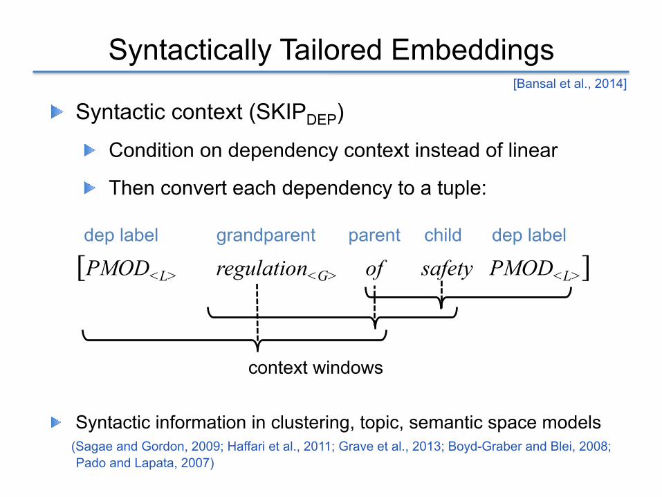
! Syntactic context (SKIPDEP)
! Condition on dependency context instead of linear
! First parse a large corpus with baseline parser:
… said that the regulation of safety is …
NMOD PMOD
(child)(parent)(grandparent)
(dep label)
[Bansal et al., 2014]
Syntactically Tailored Embeddings
dep label dep labelgrandparent parent child
[PMOD<L> regulation<G> of safety PMOD<L>]
context windows
! Syntactic context (SKIPDEP)
! Condition on dependency context instead of linear
! Then convert each dependency to a tuple:
! Syntactic information in clustering, topic, semantic space models (Sagae and Gordon, 2009; Haffari et al., 2011; Grave et al., 2013; Boyd-Graber and Blei, 2008; Pado and Lapata, 2007)
[Bansal et al., 2014]

Intrinsic Evaluation
Topical Syntactic/ Functional
(Finkelstein et al., 2002)
Representation SIM TAG
BROWN – 89.3SENNA 49.8 85.2HUANG 62.6 78.1SKIP, w = 10 44.6 71.5SKIP, w = 5 44.4 81.1SKIP, w = 1 37.8 86.6SKIPDEP 34.6 88.3
System TestBaseline 92.0SENNA (Buckets) 92.0SENNA (Hier. Clustering) 92.3HUANG (Buckets) 91.9HUANG (Hier. Clustering) 92.4
System TestBaseline 91.9BROWN 92.7SENNA 92.3TURIAN 92.3HUANG 92.4SKIP 92.3SKIPDEP 92.7
Ensemble ResultsALL – BROWN 92.9ALL 93.0
System Test Avg (5 domains)Baseline 83.5BROWN 84.2SENNA 84.3TURIAN 83.9HUANG 84.1SKIP 83.7SKIPDEP 84.1
Ensemble ResultsALL–BROWN 84.7ALL 84.9
1
[Bansal et al., 2014]
Parsing Experiments
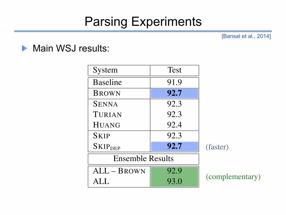
! Main WSJ results:
System TestBaseline 92.0SENNA (Buckets) 92.0SENNA (Hier. Clustering) 92.3HUANG (Buckets) 91.9HUANG (Hier. Clustering) 92.4
System TestBaseline 91.9BROWN 92.7SENNA 92.3TURIAN 92.3HUANG 92.4SKIP 92.3SKIPDEP 92.7
Ensemble ResultsALL – BROWN 92.9ALL 93.0
System Test Avg (5 domains)Baseline 83.5BROWN 84.2SENNA 84.3TURIAN 83.9HUANG 84.1SKIP 83.7SKIPDEP 84.1
Ensemble ResultsALL–BROWN 84.7ALL 84.9
1
(faster)
(complementary)
[Bansal et al., 2014]

Task-Trained Embeddings
! Can also directly train word embeddings on the task, via back-prop from the task supervision (XE errors), e.g., dependency parsing:
[Chen and Manning, 2014; CS224n] ChristopherManning
ModelArchitecture
Input layer xlookup+concat
Hidden layer hh = ReLU(Wx + b1)
Output layer yy = softmax(Uh + b2)
Softmax probabilities
cross-entropy error will beback-propagated to the embeddings.
Multilingual Embeddings via CCA
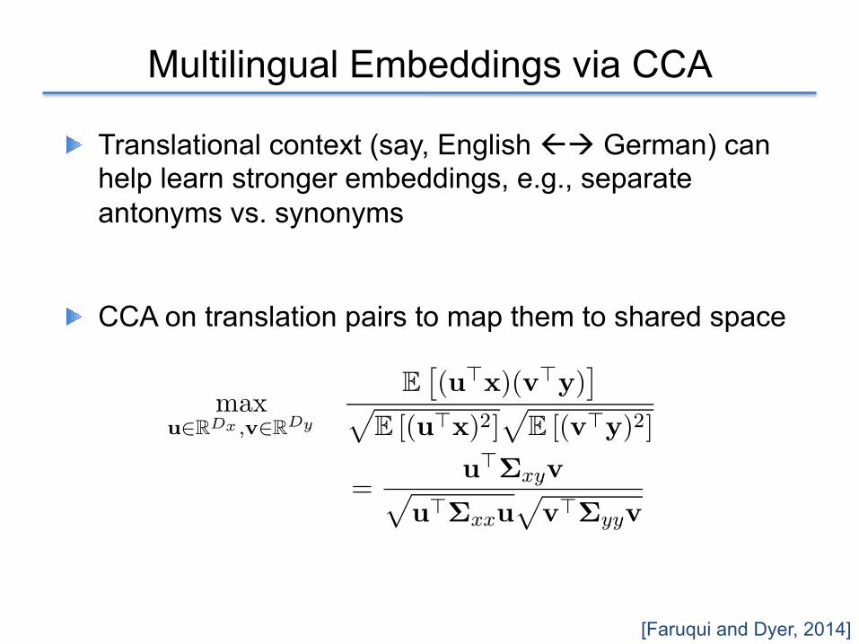
! Translational context (say, English "! German) can help learn stronger embeddings, e.g., separate antonyms vs. synonyms
! CCA on translation pairs to map them to shared space
[Faruqui and Dyer, 2014]
word�vector�2English German
word�vector�1
View 1
Vie
w2
u v
f g
foulfoul
awful
ugly
pretty
charming
cute
gorgeous
marvelous
magnificent
elegant
splendidhidous
beastlygrotesque
horrid
schrecklichen
hassliche
ziemlich
bezaubernder
cleverblondenwunderbaren
großartigeelegante
hervorragende
abscheulichen
gebotgrotesk
aufzuklaren
Figure 1: Illustration of deep CCA.
transformations of each view via deep networks.
2.1 Canonical Correlation Analysis
A popular method for multi-view representation
learning is canonical correlation analysis (CCA;
Hotelling, 1936). Its objective is to find two vec-
tors u ∈ RDx and v ∈ RDy such that projections
of the two views onto these vectors are maximally
(linearly) correlated:
maxu∈RDx ,v∈RDy
E!
(u⊤x)(v⊤y)"
#
E [(u⊤x)2]#
E [(v⊤y)2]
=u⊤Σxyv
#
u⊤Σxxu#
v⊤Σyyv(1)
where Σxy and Σxx are the cross-view and within-
view covariance matrices. (1) is extended to learn-
ing multi-dimensional projections by optimizing the
sum of correlations in all dimensions, subject to
different projected dimensions being uncorrelated.
Given sample pairs {(xi,yi)}Ni=1, the empirical es-
timates of the covariance matrices are Σxx =1
N
$Ni=1
xix⊤i + rxI, Σyy = 1
N
$Ni=1
yiy⊤i + ryI
and Σxy = 1
N
$Ni=1
xiy⊤i where (rx, ry) > 0 are
regularization parameters (Hardoon et al., 2004;
De Bie and De Moor, 2003). Then the optimal k-
dimensional projection mappings are given in closed
form via the rank-k singular value decomposition
(SVD) of the Dx×Dy matrix Σ−1/2xx ΣxyΣ
−1/2yy . In a
latent variable model interpretation of CCA, the pro-
jections reconstruct the latent variables that generate
both views (Bach and Jordan, 2005).
2.2 Deep Canonical Correlation Analysis
A linear feature mapping is often not sufficiently
powerful to faithfully capture the hidden, non-linear
relationships within the data. Recently, Andrew et
al. (2013) proposed a nonlinear extension of CCA
using deep neural networks, dubbed deep canonical
correlation analysis (DCCA) and illustrated in Fig-
ure 1. In this model, two (possibly deep) neural
networks f and g are used to extract features from
each view, and trained to maximize the correlations
between outputs in the two views, measured by a
linear CCA step with projection mappings (u,v).The neural network weights and the linear projec-
tions are optimized together using the objective
maxWf ,Wg,u,v
u⊤Σfgv#
u⊤Σffu#
v⊤Σggv, (2)
where Wf and Wg denote the weight parameters of
the two networks, and where Σfg , Σff and Σgg are
covariance matrices computed for {f(xi),g(yi)}Ni=1
in the same way as CCA. The final feature transfor-
mation is the composition of the neural network and
CCA projection, e.g., u⊤f(x) for the first view. Al-
though DCCA does not have a closed-form solution
like linear CCA, the parameters can be learned via
gradient-based optimization, whether with batch al-
gorithms like L-BFGS as in Andrew et al. (2013)
or with a stochastic gradient descent-like approach
as we do here. In each step of our SGD-like ap-
proach, we randomly select a large subset of input
samples (mini-batch), feed them forward through
the networks, and estimate the covariance matrices
and (u,v) based on these samples, so as to obtain
a stochastic version of the gradient. We then use
these stochastic gradients to update the neural net-
work weights via backpropagation.
An alternative nonlinear extension of CCA is ker-
nel CCA (KCCA) (Lai and Fyfe, 2000; Vinokourov
et al., 2003), which introduces nonlinearity through
kernels rather than neural networks. DCCA scales
better with data size, as KCCA requires computing
the SVD of a N × N matrix, and Andrew et al.
(2013) showed that DCCA achieves better total cor-
relation on held-out data than CCA or KCCA.
3 Experiments
We use English and German as the two languages.
The monolingual input word vectors are the same
as those of (Faruqui and Dyer, 2014).1 These in-
1Thanks to Faruqui and Dyer for sharing their data.

Multi-view Embeddings via CCA
[Faruqui and Dyer, 2014]
Lang Dim WS-353 WS-SIM WS-REL RG-65 MC-30 MTurk-287 SEM-REL SYN-RELEn 640 46.7 56.2 36.5 50.7 42.3 51.2 14.5 36.8
De-En 512 68.0 74.4 64.6 75.5 81.9 53.6 43.9 45.5
Fr-En 512 68.4 73.3 65.7 73.5 81.3 55.5 43.9 44.3Es-En 512 67.2 71.6 64.5 70.5 78.2 53.6 44.2 44.5
Average – 56.6 64.5 51.0 62.0 65.5 60.8 44 44.7
Table 1: Spearman’s correlation (left) and accuracy (right) on different tasks.
Figure 2: Monolingual (top) and multilingual (bottom; marked with apostrophe) word projections of theantonyms (shown in red) and synonyms of “beautiful”.
5.4 Qualitative Example
To understand how multilingual evidence leads tobetter results in semantic evaluation tasks, we plotthe word representations obtained in §3 of sev-eral synonyms and antonyms of the word “beau-tiful” by projecting both the transformed and un-transformed vectors onto R2 using the t-SNEtool (van der Maaten and Hinton, 2008). Theuntransformed LSA vectors are in the upper partof Fig. 2, and the CCA-projected vectors are inthe lower part. By comparing the two regions,we see that in the untransformed representations,the antonyms are in two clusters separated by thesynonyms, whereas in the transformed representa-tion, both the antonyms and synonyms are in theirown cluster. Furthermore, the average intra-classdistance between synonyms and antonyms is re-duced.
Figure 3: Performance of monolingual and mul-tilingual vectors on WS-353 for different vectorlengths.
5.5 Variation in Vector Length
In order to demonstrate that the gains in perfor-mance by using multilingual correlation sustains
Before CCA
After CCA
Linear vs Deep CCA
Embeddings WS-353 WS-SIM WS-REL SL-999 AN NN VN Avg
Original 46.7 56.3 36.6 26.5 26.5 38.1 34.1 32.9
CCA-1 67.2 73.0 63.4 40.7 42.4 48.1 37.4 42.6
CCA-Ens 67.5 73.1 63.7 40.4 42.0 48.2 37.8 42.7
DCCA-1 (BestAvg) 69.6 73.9 65.6 38.9 35.0 40.9 41.3 39.1
DCCA-Ens (BestAvg) 70.8 75.2 67.3 41.7 42.4 45.7 40.1 42.7
DCCA-1 (MostBeat) 68.6 73.5 65.7 42.3 44.4 44.7 36.7 41.9
DCCA-Ens (MostBeat) 69.9 74.4 66.7 42.3 43.7 47.4 38.8 43.3
Table 1: Main results on word and bigram similarity tasks, tuned on the 7 dev tasks. Shading indicates a result thatmatches or improves the best linear CCA result; boldface indicates the best result in a given column.
put embeddings are 640-dimensional and are trained
via latent semantic analysis (LSA) on the WMT
2011 monolingual news corpora.2 We use German-
English translation pairs as the input to CCA and
DCCA, using the same pairs as used by Faruqui and
Dyer. These were obtained using the word aligner
in cdec (Dyer et al., 2010) run on the WMT06-
10 news commentary corpora and Europarl. After
training, we apply the learned CCA/DCCA projec-
tion mappings to the original English word embed-
dings (180K words) and use these transformed em-
beddings for our evaluation tasks.
3.1 Evaluation Tasks
We use WordSim-353 (Finkelstein et al., 2001),
which contains 353 English word pairs with human
similarity ratings. This dataset is further divided
into two datasets WS-SIM and WS-REL by Agirre
et al. (2009) to measure similarity and relatedness.
We also use SimLex-999 (Hill et al., 2014), a new
similarity-focused dataset consisting of 666 noun-
noun pairs, 222 verb-verb pairs, and 111 adjective-
adjective pairs. Finally, we use the bigram similarity
dataset from Mitchell and Lapata (2010) which has 3
subsets, adjective-noun (AN), noun-noun (NN), and
verb-object (VN), and dev and test sets for each (of
size 649/1297 pairs). For the bigram similarity task,
we simply add the word vectors output by CCA or
DCCA to get bigram vectors.3
All of our task datasets contain pairs with human
similarity ratings. To evaluate embeddings, we com-
pute cosine similarity between the two vectors in
2http://www.statmt.org/wmt11/translation-task.html3We also tried multiplication but it performed worse. In fu-
ture work, we will directly train on bigram translation pairs.
each pair, order the pairs by similarity, and com-
pute Spearman’s correlation (ρ) between the model’s
ranking and human ranking.
Embeddings AN NN VN Avg
CCA 42.4 48.1 37.4 42.6
Deep CCA 45.5 47.1 45.1 45.9
Table 2: Bigram results, tuned on bigram dev sets.
3.2 Training and Tuning
We compare our DCCA-based embeddings to
the original word vectors and to CCA-based
embeddings. For both CCA and DCCA, we
tune the output dimensionality among factors in
{0.2, 0.4, 0.6, 0.8, 1.0} of the original embedding
dimension (640), and regularization (rx, ry) from
{10−6, 10−5, 10−4, 10−3}, based on the 7 tuning
tasks discussed below.
For training DCCA, we use stochastic gradient
descent (SGD) optimization as described in Sec-
tion 2.2. We tune SGD hyperparameters on a small
grid for fast convergence, choosing a mini-batch
size of 3000, learning rate of 0.0001, and momen-
tum of 0.99. We use rectified linear units for each
hidden layer, tuning the hidden layer width among
{128, 256, 512, 1024, 2048, 4096} and the number
of hidden layers from 1 to 4.
Our main results are based on tuning the hyperpa-
rameters (of CCA and DCCA) on 7 standard word
similarity tasks: RG-65 (Rubenstein and Goode-
nough, 1965), MC-30 (Miller and Charles, 1991),
MTurk-287 (Radinsky et al., 2011), MTurk-7714,
MEN (Bruni et al., 2014), Rare Word (Luong et al.,
4http://www2.mta.ac.il/ gideon/mturk771.html
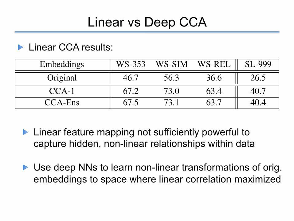
! Linear feature mapping not sufficiently powerful to capture hidden, non-linear relationships within data
! Use deep NNs to learn non-linear transformations of orig. embeddings to space where linear correlation maximized
! Linear CCA results:
Deep-CCA
word�vector�2English German
word�vector�1
View 1
Vie
w2
u v
f g
foulfoul
awful
ugly
pretty
charming
cute
gorgeous
marvelous
magnificent
elegant
splendidhidous
beastlygrotesque
horrid
schrecklichen
hassliche
ziemlich
bezaubernder
cleverblondenwunderbaren
großartigeelegante
hervorragende
abscheulichen
gebotgrotesk
aufzuklaren
Figure 1: Illustration of deep CCA.
transformations of each view via deep networks.
2.1 Canonical Correlation Analysis
A popular method for multi-view representation
learning is canonical correlation analysis (CCA;
Hotelling, 1936). Its objective is to find two vec-
tors u ∈ RDx and v ∈ RDy such that projections
of the two views onto these vectors are maximally
(linearly) correlated:
maxu∈RDx ,v∈RDy
E!
(u⊤x)(v⊤y)"
#
E [(u⊤x)2]#
E [(v⊤y)2]
=u⊤Σxyv
#
u⊤Σxxu#
v⊤Σyyv(1)
where Σxy and Σxx are the cross-view and within-
view covariance matrices. (1) is extended to learn-
ing multi-dimensional projections by optimizing the
sum of correlations in all dimensions, subject to
different projected dimensions being uncorrelated.
Given sample pairs {(xi,yi)}Ni=1, the empirical es-
timates of the covariance matrices are Σxx =1
N
$Ni=1
xix⊤i + rxI, Σyy = 1
N
$Ni=1
yiy⊤i + ryI
and Σxy = 1
N
$Ni=1
xiy⊤i where (rx, ry) > 0 are
regularization parameters (Hardoon et al., 2004;
De Bie and De Moor, 2003). Then the optimal k-
dimensional projection mappings are given in closed
form via the rank-k singular value decomposition
(SVD) of the Dx×Dy matrix Σ−1/2xx ΣxyΣ
−1/2yy . In a
latent variable model interpretation of CCA, the pro-
jections reconstruct the latent variables that generate
both views (Bach and Jordan, 2005).
2.2 Deep Canonical Correlation Analysis
A linear feature mapping is often not sufficiently
powerful to faithfully capture the hidden, non-linear
relationships within the data. Recently, Andrew et
al. (2013) proposed a nonlinear extension of CCA
using deep neural networks, dubbed deep canonical
correlation analysis (DCCA) and illustrated in Fig-
ure 1. In this model, two (possibly deep) neural
networks f and g are used to extract features from
each view, and trained to maximize the correlations
between outputs in the two views, measured by a
linear CCA step with projection mappings (u,v).The neural network weights and the linear projec-
tions are optimized together using the objective
maxWf ,Wg,u,v
u⊤Σfgv#
u⊤Σffu#
v⊤Σggv, (2)
where Wf and Wg denote the weight parameters of
the two networks, and where Σfg , Σff and Σgg are
covariance matrices computed for {f(xi),g(yi)}Ni=1
in the same way as CCA. The final feature transfor-
mation is the composition of the neural network and
CCA projection, e.g., u⊤f(x) for the first view. Al-
though DCCA does not have a closed-form solution
like linear CCA, the parameters can be learned via
gradient-based optimization, whether with batch al-
gorithms like L-BFGS as in Andrew et al. (2013)
or with a stochastic gradient descent-like approach
as we do here. In each step of our SGD-like ap-
proach, we randomly select a large subset of input
samples (mini-batch), feed them forward through
the networks, and estimate the covariance matrices
and (u,v) based on these samples, so as to obtain
a stochastic version of the gradient. We then use
these stochastic gradients to update the neural net-
work weights via backpropagation.
An alternative nonlinear extension of CCA is ker-
nel CCA (KCCA) (Lai and Fyfe, 2000; Vinokourov
et al., 2003), which introduces nonlinearity through
kernels rather than neural networks. DCCA scales
better with data size, as KCCA requires computing
the SVD of a N × N matrix, and Andrew et al.
(2013) showed that DCCA achieves better total cor-
relation on held-out data than CCA or KCCA.
3 Experiments
We use English and German as the two languages.
The monolingual input word vectors are the same
as those of (Faruqui and Dyer, 2014).1 These in-
1Thanks to Faruqui and Dyer for sharing their data.
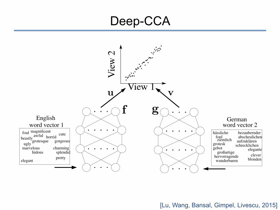
[Lu, Wang, Bansal, Gimpel, Livescu, 2015]

Deep-CCA
! 2 DNNs f, g extract features from the 2 input views x and y
! DNNs are trained to maximize output linear correlation of 2 views ! DNN weights and linear projections optimized together:
! Covariance matrices computed for , as in CCA ! Mini-batch SGD: Feed-forward a sample to estimate (u, v) and
gradient and then update NN weights via back-propagation
word�vector�2English German
word�vector�1
View 1
Vie
w2
u v
f g
foulfoul
awful
ugly
pretty
charming
cute
gorgeous
marvelous
magnificent
elegant
splendidhidous
beastlygrotesque
horrid
schrecklichen
hassliche
ziemlich
bezaubernder
cleverblondenwunderbaren
großartigeelegante
hervorragende
abscheulichen
gebotgrotesk
aufzuklaren
Figure 1: Illustration of deep CCA.
transformations of each view via deep networks.
2.1 Canonical Correlation Analysis
A popular method for multi-view representation
learning is canonical correlation analysis (CCA;
Hotelling, 1936). Its objective is to find two vec-
tors u ∈ RDx and v ∈ RDy such that projections
of the two views onto these vectors are maximally
(linearly) correlated:
maxu∈RDx ,v∈RDy
E!
(u⊤x)(v⊤y)"
#
E [(u⊤x)2]#
E [(v⊤y)2]
=u⊤Σxyv
#
u⊤Σxxu#
v⊤Σyyv(1)
where Σxy and Σxx are the cross-view and within-
view covariance matrices. (1) is extended to learn-
ing multi-dimensional projections by optimizing the
sum of correlations in all dimensions, subject to
different projected dimensions being uncorrelated.
Given sample pairs {(xi,yi)}Ni=1, the empirical es-
timates of the covariance matrices are Σxx =1
N
$Ni=1
xix⊤i + rxI, Σyy = 1
N
$Ni=1
yiy⊤i + ryI
and Σxy = 1
N
$Ni=1
xiy⊤i where (rx, ry) > 0 are
regularization parameters (Hardoon et al., 2004;
De Bie and De Moor, 2003). Then the optimal k-
dimensional projection mappings are given in closed
form via the rank-k singular value decomposition
(SVD) of the Dx×Dy matrix Σ−1/2xx ΣxyΣ
−1/2yy . In a
latent variable model interpretation of CCA, the pro-
jections reconstruct the latent variables that generate
both views (Bach and Jordan, 2005).
2.2 Deep Canonical Correlation Analysis
A linear feature mapping is often not sufficiently
powerful to faithfully capture the hidden, non-linear
relationships within the data. Recently, Andrew et
al. (2013) proposed a nonlinear extension of CCA
using deep neural networks, dubbed deep canonical
correlation analysis (DCCA) and illustrated in Fig-
ure 1. In this model, two (possibly deep) neural
networks f and g are used to extract features from
each view, and trained to maximize the correlations
between outputs in the two views, measured by a
linear CCA step with projection mappings (u,v).The neural network weights and the linear projec-
tions are optimized together using the objective
maxWf ,Wg,u,v
u⊤Σfgv#
u⊤Σffu#
v⊤Σggv, (2)
where Wf and Wg denote the weight parameters of
the two networks, and where Σfg , Σff and Σgg are
covariance matrices computed for {f(xi),g(yi)}Ni=1
in the same way as CCA. The final feature transfor-
mation is the composition of the neural network and
CCA projection, e.g., u⊤f(x) for the first view. Al-
though DCCA does not have a closed-form solution
like linear CCA, the parameters can be learned via
gradient-based optimization, whether with batch al-
gorithms like L-BFGS as in Andrew et al. (2013)
or with a stochastic gradient descent-like approach
as we do here. In each step of our SGD-like ap-
proach, we randomly select a large subset of input
samples (mini-batch), feed them forward through
the networks, and estimate the covariance matrices
and (u,v) based on these samples, so as to obtain
a stochastic version of the gradient. We then use
these stochastic gradients to update the neural net-
work weights via backpropagation.
An alternative nonlinear extension of CCA is ker-
nel CCA (KCCA) (Lai and Fyfe, 2000; Vinokourov
et al., 2003), which introduces nonlinearity through
kernels rather than neural networks. DCCA scales
better with data size, as KCCA requires computing
the SVD of a N × N matrix, and Andrew et al.
(2013) showed that DCCA achieves better total cor-
relation on held-out data than CCA or KCCA.
3 Experiments
We use English and German as the two languages.
The monolingual input word vectors are the same
as those of (Faruqui and Dyer, 2014).1 These in-
1Thanks to Faruqui and Dyer for sharing their data.
[Andrew et al., 2013]
word�vector�2English German
word�vector�1
View 1
Vie
w2
u v
f g
foulfoul
awful
ugly
pretty
charming
cute
gorgeous
marvelous
magnificent
elegant
splendidhidous
beastlygrotesque
horrid
schrecklichen
hassliche
ziemlich
bezaubernder
cleverblondenwunderbaren
großartigeelegante
hervorragende
abscheulichen
gebotgrotesk
aufzuklaren
Figure 1: Illustration of deep CCA.
transformations of each view via deep networks.
2.1 Canonical Correlation Analysis
A popular method for multi-view representation
learning is canonical correlation analysis (CCA;
Hotelling, 1936). Its objective is to find two vec-
tors u ∈ RDx and v ∈ RDy such that projections
of the two views onto these vectors are maximally
(linearly) correlated:
maxu∈RDx ,v∈RDy
E!
(u⊤x)(v⊤y)"
#
E [(u⊤x)2]#
E [(v⊤y)2]
=u⊤Σxyv
#
u⊤Σxxu#
v⊤Σyyv(1)
where Σxy and Σxx are the cross-view and within-
view covariance matrices. (1) is extended to learn-
ing multi-dimensional projections by optimizing the
sum of correlations in all dimensions, subject to
different projected dimensions being uncorrelated.
Given sample pairs {(xi,yi)}Ni=1, the empirical es-
timates of the covariance matrices are Σxx =1
N
$Ni=1
xix⊤i + rxI, Σyy = 1
N
$Ni=1
yiy⊤i + ryI
and Σxy = 1
N
$Ni=1
xiy⊤i where (rx, ry) > 0 are
regularization parameters (Hardoon et al., 2004;
De Bie and De Moor, 2003). Then the optimal k-
dimensional projection mappings are given in closed
form via the rank-k singular value decomposition
(SVD) of the Dx×Dy matrix Σ−1/2xx ΣxyΣ
−1/2yy . In a
latent variable model interpretation of CCA, the pro-
jections reconstruct the latent variables that generate
both views (Bach and Jordan, 2005).
2.2 Deep Canonical Correlation Analysis
A linear feature mapping is often not sufficiently
powerful to faithfully capture the hidden, non-linear
relationships within the data. Recently, Andrew et
al. (2013) proposed a nonlinear extension of CCA
using deep neural networks, dubbed deep canonical
correlation analysis (DCCA) and illustrated in Fig-
ure 1. In this model, two (possibly deep) neural
networks f and g are used to extract features from
each view, and trained to maximize the correlations
between outputs in the two views, measured by a
linear CCA step with projection mappings (u,v).The neural network weights and the linear projec-
tions are optimized together using the objective
maxWf ,Wg,u,v
u⊤Σfgv#
u⊤Σffu#
v⊤Σggv, (2)
where Wf and Wg denote the weight parameters of
the two networks, and where Σfg , Σff and Σgg are
covariance matrices computed for {f(xi),g(yi)}Ni=1
in the same way as CCA. The final feature transfor-
mation is the composition of the neural network and
CCA projection, e.g., u⊤f(x) for the first view. Al-
though DCCA does not have a closed-form solution
like linear CCA, the parameters can be learned via
gradient-based optimization, whether with batch al-
gorithms like L-BFGS as in Andrew et al. (2013)
or with a stochastic gradient descent-like approach
as we do here. In each step of our SGD-like ap-
proach, we randomly select a large subset of input
samples (mini-batch), feed them forward through
the networks, and estimate the covariance matrices
and (u,v) based on these samples, so as to obtain
a stochastic version of the gradient. We then use
these stochastic gradients to update the neural net-
work weights via backpropagation.
An alternative nonlinear extension of CCA is ker-
nel CCA (KCCA) (Lai and Fyfe, 2000; Vinokourov
et al., 2003), which introduces nonlinearity through
kernels rather than neural networks. DCCA scales
better with data size, as KCCA requires computing
the SVD of a N × N matrix, and Andrew et al.
(2013) showed that DCCA achieves better total cor-
relation on held-out data than CCA or KCCA.
3 Experiments
We use English and German as the two languages.
The monolingual input word vectors are the same
as those of (Faruqui and Dyer, 2014).1 These in-
1Thanks to Faruqui and Dyer for sharing their data.

Results
Embeddings WS-353 WS-SIM WS-REL SL-999 AN NN VN Avg
Original 46.7 56.3 36.6 26.5 26.5 38.1 34.1 32.9
CCA-1 67.2 73.0 63.4 40.7 42.4 48.1 37.4 42.6
CCA-Ens 67.5 73.1 63.7 40.4 42.0 48.2 37.8 42.7
DCCA-1 (BestAvg) 69.6 73.9 65.6 38.9 35.0 40.9 41.3 39.1
DCCA-Ens (BestAvg) 70.8 75.2 67.3 41.7 42.4 45.7 40.1 42.7
DCCA-1 (MostBeat) 68.6 73.5 65.7 42.3 44.4 44.7 36.7 41.9
DCCA-Ens (MostBeat) 69.9 74.4 66.7 42.3 43.7 47.4 38.8 43.3
Table 1: Main results on word and bigram similarity tasks, tuned on the 7 dev tasks. Shading indicates a result thatmatches or improves the best linear CCA result; boldface indicates the best result in a given column.
put embeddings are 640-dimensional and are trained
via latent semantic analysis (LSA) on the WMT
2011 monolingual news corpora.2 We use German-
English translation pairs as the input to CCA and
DCCA, using the same pairs as used by Faruqui and
Dyer. These were obtained using the word aligner
in cdec (Dyer et al., 2010) run on the WMT06-
10 news commentary corpora and Europarl. After
training, we apply the learned CCA/DCCA projec-
tion mappings to the original English word embed-
dings (180K words) and use these transformed em-
beddings for our evaluation tasks.
3.1 Evaluation Tasks
We use WordSim-353 (Finkelstein et al., 2001),
which contains 353 English word pairs with human
similarity ratings. This dataset is further divided
into two datasets WS-SIM and WS-REL by Agirre
et al. (2009) to measure similarity and relatedness.
We also use SimLex-999 (Hill et al., 2014), a new
similarity-focused dataset consisting of 666 noun-
noun pairs, 222 verb-verb pairs, and 111 adjective-
adjective pairs. Finally, we use the bigram similarity
dataset from Mitchell and Lapata (2010) which has 3
subsets, adjective-noun (AN), noun-noun (NN), and
verb-object (VN), and dev and test sets for each (of
size 649/1297 pairs). For the bigram similarity task,
we simply add the word vectors output by CCA or
DCCA to get bigram vectors.3
All of our task datasets contain pairs with human
similarity ratings. To evaluate embeddings, we com-
pute cosine similarity between the two vectors in
2http://www.statmt.org/wmt11/translation-task.html3We also tried multiplication but it performed worse. In fu-
ture work, we will directly train on bigram translation pairs.
each pair, order the pairs by similarity, and com-
pute Spearman’s correlation (ρ) between the model’s
ranking and human ranking.
Embeddings AN NN VN Avg
CCA 42.4 48.1 37.4 42.6
Deep CCA 45.5 47.1 45.1 45.9
Table 2: Bigram results, tuned on bigram dev sets.
3.2 Training and Tuning
We compare our DCCA-based embeddings to
the original word vectors and to CCA-based
embeddings. For both CCA and DCCA, we
tune the output dimensionality among factors in
{0.2, 0.4, 0.6, 0.8, 1.0} of the original embedding
dimension (640), and regularization (rx, ry) from
{10−6, 10−5, 10−4, 10−3}, based on the 7 tuning
tasks discussed below.
For training DCCA, we use stochastic gradient
descent (SGD) optimization as described in Sec-
tion 2.2. We tune SGD hyperparameters on a small
grid for fast convergence, choosing a mini-batch
size of 3000, learning rate of 0.0001, and momen-
tum of 0.99. We use rectified linear units for each
hidden layer, tuning the hidden layer width among
{128, 256, 512, 1024, 2048, 4096} and the number
of hidden layers from 1 to 4.
Our main results are based on tuning the hyperpa-
rameters (of CCA and DCCA) on 7 standard word
similarity tasks: RG-65 (Rubenstein and Goode-
nough, 1965), MC-30 (Miller and Charles, 1991),
MTurk-287 (Radinsky et al., 2011), MTurk-7714,
MEN (Bruni et al., 2014), Rare Word (Luong et al.,
4http://www2.mta.ac.il/ gideon/mturk771.html
! Word-similarity improvements
! Also gets improvements on bigram similarity datasets
[Lu, Wang, Bansal, Gimpel, Livescu, 2015]

Analysis
Embeddings WS-353 WS-SIM WS-REL SL-999 AN NN VN Avg Dim
Original 46.7 56.3 36.6 26.5 26.5 38.1 34.1 32.9 640
CCA-1 67.2 73.0 63.4 40.7 42.4 48.1 37.4 42.6 384
CCA-Ens 67.5 73.1 63.7 40.4 42.0 48.2 37.8 42.7 384
DCCA-1 (BestAvg) 69.6 73.9 65.6 38.9 35.0 40.9 41.3 39.1 128
DCCA-Ens (BestAvg) 70.8 75.2 67.3 41.7 42.4 45.7 40.1 42.7 128
DCCA-1 (MostBeat) 68.6 73.5 65.7 42.3 44.4 44.7 36.7 41.9 384
DCCA-Ens (MostBeat) 69.9 74.4 66.7 42.3 43.7 47.4 38.8 43.3 384
Table 1: Main results on word and bigram similarity tasks, tuned on 7 development tasks (see text for
details). Shading indicates a result that matches or improves the best linear CCA result; boldface indicates
the best result in a given column. See Section 3.4 for discussion on NN results.
Embeddings AN NN VN Avg
CCA 42.4 48.1 37.4 42.6
Deep CCA 45.5 47.1 45.1 45.9
Table 2: Bigram results, tuned on bigram dev sets.
gram tasks themselves (as provided by Mitchell and
Lapata), since the 7 tuning tasks are not particularly
related to the bigram test sets. We see that DCCA
can achieve even stronger improvements over CCA
and overall using these related dev sets.
We note that the performance on the NN task
does not improve. The typical variance of annota-
tor scores for each bigram pair was larger for the
NN dataset than for the other bigram datasets, sug-
gesting noisier annotations. Also, we found that the
NN annotations often reflected topical relatedness
rather than functional similarity, e.g., television set
and television programme are among the most simi-
lar noun-noun bigrams. We expect that multilingual
information would help embeddings to more closely
reflect functional similarity.
For DCCA, we found that the best-performing
networks were typically asymmetric, with 1 to 2 lay-
ers on the English side and 2 to 4 on the German
side. The best network structure on the bigram VN
development set is 640-128-128 for the English view
and 640-128-512-128 for the German view, with a
final CCA projection layer with dimensionality 128
for each language.
4 Discussion
Normalization and Evaluation We note that the
cosine similarity (and thus Spearman’s ρ) between a
pair of words is not invariant to the series of simple
(affine) transformations done by the normalizations
in our procedure. For their baseline, Faruqui and
Dyer (2014) did not remove the standard deviation
better with DCCA worse with DCCA
arrive come author creatorlocate find leader manager
way manner buddy companionrecent new crowd bunch
take obtain achieve succeedboundary border attention interest
win accomplish join addcontemplate think mood emotion
Table 3: Highly-similar pairs in SimLex-999 that
improved/degraded the most under DCCA. Pairs are
sorted in decreasing order according to the amount
of improvement/degradation.
of the 36K training set for the 180K English vocabu-
lary during testing. We have accidentally found that
this normalization step alone greatly improves the
performance of the original vectors.
For example, the WS-353 correlation improves
from 46.7 to 67.1, essentially matching the linear
CCA correlations, though DCCA still outperforms
them both. This indicates that the cosine similarity
is not stable, and it is likely better to learn a dis-
tance/similarity function (using labeled tuning data)
atop the learned features such that similarities be-
tween selected pairs will match the human similari-
ties, or such that the rankings will match.
Error Analysis We analyze high-similarity word
pairs that change the most with DCCA, as compared
to both linear CCA and the original vectors.
For a word pair w, we use r(w) to refer to its
similarity rank, subscripting it whether it is com-
puted according to human ratings (rh) or if based
on cosine similarity via the original vectors (ro),
CCA-1 (rc), or DCCA-1 MostBeat (rd). We define
δa(w) = |ra(w) − rh(w)| and compute ∆(w) =
! DCCA discards hypernymy, separates senses
! High-similarity word pairs that change most with DCCA
[Lu, Wang, Bansal, Gimpel, Livescu, 2015]

Analysis
! DCCA more cleanly separates synonym-antonym lists
Original CCA-1 DCCA-1 (MostBeat)
Figure 2: t-SNE visualization of synonyms (green) and antonyms (red, capitalized) of dangerous.
δd(w) − (δc(w) + δo(w)). If ∆(w) < 0, then
word pair w was closer to the human ranking using
DCCA. Table 3 shows word pairs from SimLex-999
with high human similarity ratings (≥ 7 out of 10);
column 1 shows pairs with smallest ∆ values, and
column 2 shows pairs with largest ∆ values.
Among pairs in column 1, many contain words
with several senses. Using bilingual information is
likely to focus on the most frequent sense in the bi-
text, due to our use of the most frequently-aligned
German word in each training pair. By contrast,
using only monolingual context is expected to find
an embedding that blends the contextual information
across all word senses.
Several pairs from column 2 show hypernym
rather than paraphrase relationships, e.g., author-
creator and leader-manager. Though these pairs are
rated as highly similar by annotators, linear CCA
made them less similar than the original vectors, and
DCCA made them less similar still. This matches
our intuition that bilingual information should en-
courage paraphrase-like similarity and thereby dis-
courage the similarity of hypernym-hyponym pairs.
Visualizations We visualized several synonym-
antonym word lists and often found that DCCA
more cleanly separated synonyms from antonyms
than CCA or the original vectors. An example of
the clearest improvement is shown in Fig. 2.
5 Related work
Previous work has successfully used translational
context for word representations (Diab and Resnik,
2002; Zhao et al., 2005; Tackstrom et al., 2012;
Bansal et al., 2012; Faruqui and Dyer, 2014), includ-
ing via hand-designed vector space models (Peirs-
man and Pado, 2010; Sumita, 2000) or via unsuper-
vised LDA and LSA (Boyd-Graber and Blei, 2009;
Zhao and Xing, 2006).
There have been other recent deep learning ap-
proaches to bilingual representations, e.g., based on
a joint monolingual and bilingual objective (Zou
et al., 2013). There has also been recent interest
in learning bilingual representations without using
word alignments (Chandar et al., 2014; Gouws et al.,
2014; Kocisky et al., 2014; Vulic and Moens, 2013).
This research is also related to early examples of
learning bilingual lexicons using monolingual cor-
pora (Koehn and Knight, 2002; Haghighi et al.,
2008); the latter used CCA to find matched word
pairs. Irvine and Callison-Burch (2013) used a su-
pervised learning method with multiple monolingual
signals. Finally, other work on CCA and spectral
methods has been used in the context of other types
of views (Collobert and Weston, 2008; Dhillon et al.,
2011; Klementiev et al., 2012; Chang et al., 2013).
6 Conclusion
We have demonstrated how bilingual information
can be incorporated into word embeddings via deep
canonical correlation analysis (DCCA). The DCCA
embeddings consistently outperform linear CCA
embeddings on word and bigram similarity tasks.
Future work could compare DCCA to other non-
linear approaches discussed in §5, compare differ-
ent languages as multiview context, and extend to
aligned phrase pairs, and to unaligned data.
Acknowledgments
We are grateful to Manaal Faruqui for sharing re-
sources, and to Chris Dyer, David Sontag, Lyle Un-
gar, and anonymous reviewers for helpful input.
[Lu, Wang, Bansal, Gimpel, Livescu, 2015]

Retrofitting Word Embeddings to Lexicons
! We want the inferred word vector to be close to the observed value qˆ and close to its neighbors qj, ∀j such that (i, j) ∈ E, where E is the set of relations in a dictionary/lexicon (e.g., WordNet, PPDB, etc.)
[Faruqui et al., 2015]
Figure 1: Word graph with edges between related wordsshowing the observed (grey) and the inferred (white)word vector representations.
Experimentally, we show that our method workswell with different state-of-the-art word vector mod-els, using different kinds of semantic lexicons andgives substantial improvements on a variety ofbenchmarks, while beating the current state-of-the-art approaches for incorporating semantic informa-tion in vector training and trivially extends to mul-tiple languages. We show that retrofitting givesconsistent improvement in performance on evalua-tion benchmarks with different word vector lengthsand show a qualitative visualization of the effect ofretrofitting on word vector quality. The retrofittingtool is available at: https://github.com/
mfaruqui/retrofitting.
2 Retrofitting with Semantic Lexicons
Let V = {w1, . . . , wn} be a vocabulary, i.e, the setof word types, and⌦ be an ontology that encodes se-mantic relations between words in V . We represent⌦ as an undirected graph (V,E) with one vertex foreach word type and edges (wi, wj) 2 E ✓ V ⇥ Vindicating a semantic relationship of interest. Theserelations differ for different semantic lexicons andare described later (§4).
The matrix ˆQ will be the collection of vector rep-resentations qi 2 Rd, for each wi 2 V , learnedusing a standard data-driven technique, where d isthe length of the word vectors. Our objective isto learn the matrix Q = (q1, . . . , qn) such that thecolumns are both close (under a distance metric) totheir counterparts in ˆQ and to adjacent vertices in ⌦.Figure 1 shows a small word graph with such edgeconnections; white nodes are labeled with the Q vec-
tors to be retrofitted (and correspond to V⌦); shadednodes are labeled with the corresponding vectors inˆQ, which are observed. The graph can be interpretedas a Markov random field (Kindermann and Snell,1980).
The distance between a pair of vectors is definedto be the Euclidean distance. Since we want theinferred word vector to be close to the observedvalue qi and close to its neighbors qj , 8j such that(i, j) 2 E, the objective to be minimized becomes:
(Q) =
nX
i=1
2
4↵ikqi � qik2+
X
(i,j)2E
�ijkqi � qjk2
3
5
where ↵ and � values control the relative strengthsof associations (more details in §6.1).
In this case, we first train the word vectors inde-pendent of the information in the semantic lexiconsand then retrofit them. is convex in Q and its so-lution can be found by solving a system of linearequations. To do so, we use an efficient iterativeupdating method (Bengio et al., 2006; Subramanyaet al., 2010; Das and Petrov, 2011; Das and Smith,2011). The vectors in Q are initialized to be equalto the vectors in ˆQ. We take the first derivative of with respect to one qi vector, and by equating it tozero arrive at the following online update:
qi =
Pj:(i,j)2E �ijqj + ↵iqiP
j:(i,j)2E �ij + ↵i(1)
In practice, running this procedure for 10 iterationsconverges to changes in Euclidean distance of ad-jacent vertices of less than 10
�2. The retrofittingapproach described above is modular; it can be ap-plied to word vector representations obtained fromany model as the updates in Eq. 1 are agnostic to theoriginal vector training model objective.
Semantic Lexicons during Learning. Our pro-posed approach is reminiscent of recent work onimproving word vectors using lexical resources (Yuand Dredze, 2014; Bian et al., 2014; Xu et al., 2014)which alters the learning objective of the originalvector training model with a prior (or a regularizer)that encourages semantically related vectors (in ⌦)to be close together, except that our technique is ap-plied as a second stage of learning. We describe the

Bias in Word Embeddings
[Bolukbasi et al., 2016]
Extreme she
1. homemaker2. nurse3. receptionist4. librarian5. socialite6. hairdresser7. nanny8. bookkeeper9. stylist10. housekeeper
Extreme he
1. maestro2. skipper3. protege4. philosopher5. captain6. architect7. financier8. warrior9. broadcaster10. magician
Gender stereotype she-he analogiessewing-carpentry registered nurse-physician housewife-shopkeepernurse-surgeon interior designer-architect softball-baseballblond-burly feminism-conservatism cosmetics-pharmaceuticalsgiggle-chuckle vocalist-guitarist petite-lankysassy-snappy diva-superstar charming-affablevolleyball-football cupcakes-pizzas lovely-brilliant
Gender appropriate she-he analogiesqueen-king sister-brother mother-fatherwaitress-waiter ovarian cancer-prostate cancer convent-monastery
Figure 1: Left The most extreme occupations as projected on to the she�he gender direction onw2vNEWS. Occupations such as businesswoman, where gender is suggested by the orthography,were excluded. Right Automatically generated analogies for the pair she-he using the proceduredescribed in text. Each automatically generated analogy is evaluated by 10 crowd-workers to whetheror not it reflects gender stereotype.
father is to a doctor as a mother is to a nurse. The primary embedding studied in this paper is thepopular publicly-available word2vec [19, 20] 300 dimensional embedding trained on a corpus ofGoogle News texts consisting of 3 million English words, which we refer to here as the w2vNEWS.One might have hoped that the Google News embedding would exhibit little gender bias becausemany of its authors are professional journalists. We also analyze other publicly available embeddingstrained via other algorithms and find similar biases (Appendix B).
In this paper, we quantitatively demonstrate that word-embeddings contain biases in their geometrythat reflect gender stereotypes present in broader society.1 Due to their wide-spread usage as basicfeatures, word embeddings not only reflect such stereotypes but can also amplify them. This poses asignificant risk and challenge for machine learning and its applications. The analogies generated fromthese embeddings spell out the bias implicit in the data on which they were trained. Hence, wordembeddings may serve as a means to extract implicit gender associations from a large text corpussimilar to how Implicit Association Tests [11] detect automatic gender associations possessed bypeople, which often do not align with self reports.
To quantify bias, we will compare a word vector to the vectors of a pair of gender-specific words. Forinstance, the fact that ���!nurse is close to ����!woman is not in itself necessarily biased(it is also somewhatclose to ��!man – all are humans), but the fact that these distances are unequal suggests bias. To makethis rigorous, consider the distinction between gender specific words that are associated with a genderby definition, and the remaining gender neutral words. Standard examples of gender specific wordsinclude brother, sister, businessman and businesswoman. We will use the gender specific words tolearn a gender subspace in the embedding, and our debiasing algorithm removes the bias only fromthe gender neutral words while respecting the definitions of these gender specific words.
We propose approaches to reduce gender biases in the word embedding while preserving the usefulproperties of the embedding. Surprisingly, not only does the embedding capture bias, but it alsocontains sufficient information to reduce this bias.We will leverage the fact that there exists a lowdimensional subspace in the embedding that empirically captures much of the gender bias.
2 Related work and PreliminaryGender bias and stereotype in English. It is important to quantify and understand bias in languagesas such biases can reinforce the psychological status of different groups [28]. Gender bias in languagehas been studied over a number of decades in a variety of contexts (see, e.g., [13]) and we onlyhighlight some of the findings here. Biases differ across people though commonalities can be detected.Implicit Association Tests [11] have uncovered gender-word biases that people do not self-report andmay not even be aware of. Common biases link female terms with liberal arts and family and maleterms with science and careers [23]. Bias is seen in word morphology, i.e., the fact that words such as
1 Stereotypes are biases that are widely held among a group of people. We show that the biases in the wordembedding are in fact closely aligned with social conception of gender stereotype, as evaluated by U.S.-basedcrowd workers on Amazon’s Mechanical Turk. The crowd agreed that the biases reflected both in the location ofvectors (e.g.
���!doctor closer to ��!man than to ����!woman) as well as in analogies (e.g., he:coward :: she:whore.) exhibit
common gender stereotypes.
2
! Debiasing word embeddings via identifying pairs (sets) of words to correct/neutralize, identify bias direction (subspace), and then debias via neutralize+equalize or soften algorithms.

Compositional Semantics with NNs
! Composing, combining word vectors to representations for longer units: phrases, sentences, paragraphs, …
! Initial approaches: point-wise sum, multiplication [Mitchell and Lapata, 2010; Blacoe and Lapata, 2012]
! Vector-matrix compositionality [Baroni and Zamparelli, 2010; Zanzotto et al., 2010; Grefenstette and Sadrzadeh, 2011; Socher et al., 2011; Yessenalina and Cardie, 2011]
! Linguistic information added via say parses in RvNNs [Socher et al., 2011b, 2012, 2013a, 2013b, 2014; Hermann and Blunsom, 2013]
! Sequential RNNs (with GRU/LSTM gates) (Simple vector averaging w/ updating sometimes competitive)

Compositional Semantics with NNs
! Feed-forward NNs with back-propagation
Softmax (=logisticregression)isnotverypowerful
4/7/16RichardSocher29
• Softmax onlylineardecisionboundaries
• à Lamewhenproblemiscomplex
• Wouldn’titbecooltogetthesecorrect?
NN and backprop slides from CS224d – Richard Socher

Compositional Semantics with NNs
! Feed-forward NNs with back-propagation
NeuralNetsfortheWin!
4/7/16RichardSocher30
• Neuralnetworkscanlearnmuchmorecomplexfunctionsandnonlineardecisionboundaries!
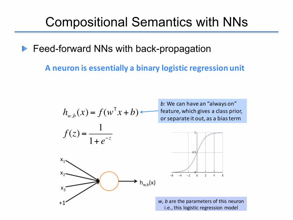
Compositional Semantics with NNs
! Feed-forward NNs with back-propagation
Aneuronisessentiallyabinarylogisticregressionunit
hw,b(x) = f (wTx + b)
f (z) = 11+ e−z
w,b aretheparametersofthisneuroni.e.,thislogisticregressionmodel
33
b:Wecanhavean“alwayson”feature,whichgivesaclassprior,orseparateitout,asabiasterm

Compositional Semantics with NNs
! Feed-forward NNs with back-propagation
Aneuralnetwork=runningseverallogisticregressionsatthesametimeBeforeweknowit,wehaveamultilayerneuralnetwork….
36

Compositional Semantics with NNs
! Feed-forward NNs with back-propagation
TrainingwithBackpropagation
• Let’sconsiderthederivativeofasingleweightWij
• Thisonlyappearsinsideai
• Forexample:W23 isonlyusedtocomputea2
x1 x2x3 +1
a1 a2
s U2
W23
19
b2
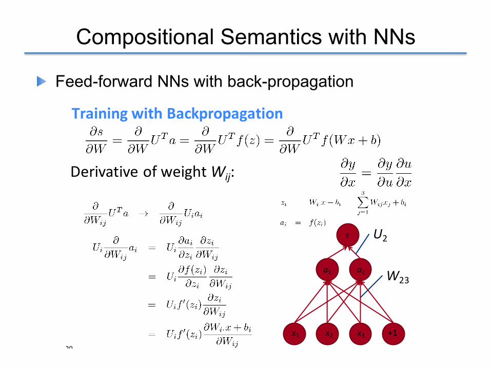
Compositional Semantics with NNs
! Feed-forward NNs with back-propagation
TrainingwithBackpropagation
DerivativeofweightWij:
20
x1 x2x3 +1
a1 a2
s U2
W23
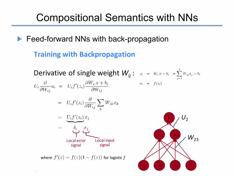
Compositional Semantics with NNs
! Feed-forward NNs with back-propagation
whereforlogisticf
TrainingwithBackpropagation
DerivativeofsingleweightWij :
Localerrorsignal
Localinputsignal
21
x1 x2x3 +1
a1 a2
s U2
W23

Syntactically Recursive NNs
! Socher et al., 2013a, 2014: RvNNs on constituent and dependency parse trees
Figure 2: An example tree with a simple RecursiveNeural Network: The same weight matrix is repli-cated and used to compute all non-terminal noderepresentations. Leaf nodes are n-dimensionalvector representations of words.
In order to compute a score of how plausible ofa syntactic constituent a parent is the RNN uses asingle-unit linear layer for all i:
s(p
(i)
) = v
T
p
(i)
,
where v 2 Rn is a vector of parameters that needto be trained. This score will be used to find thehighest scoring tree. For more details on how stan-dard RNNs can be used for parsing, see Socher etal. (2011b).
The standard RNN requires a single composi-tion function to capture all types of compositions:adjectives and nouns, verbs and nouns, adverbsand adjectives, etc. Even though this function isa powerful one, we find a single neural networkweight matrix cannot fully capture the richness ofcompositionality. Several extensions are possible:A two-layered RNN would provide more expres-sive power, however, it is much harder to train be-cause the resulting neural network becomes verydeep and suffers from vanishing gradient prob-lems. Socher et al. (2012) proposed to give ev-ery single word a matrix and a vector. The ma-trix is then applied to the sibling node’s vectorduring the composition. While this results in apowerful composition function that essentially de-pends on the words being combined, the numberof model parameters explodes and the composi-tion functions do not capture the syntactic com-monalities between similar POS tags or syntacticcategories.
Based on the above considerations, we proposethe Compositional Vector Grammar (CVG) thatconditions the composition function at each nodeon discrete syntactic categories extracted from a
(A, a= ) (B, b= ) (C, c= )
P(1), p(1)=
P(2), p(2)=
= f W(B,C) bc
= f W(A,P ) ap(1)
(1)
Figure 3: Example of a syntactically untied RNNin which the function to compute a parent vectordepends on the syntactic categories of its childrenwhich we assume are given for now.
PCFG. Hence, CVGs combine discrete, syntacticrule probabilities and continuous vector composi-tions. The idea is that the syntactic categories ofthe children determine what composition functionto use for computing the vector of their parents.While not perfect, a dedicated composition func-tion for each rule RHS can well capture commoncomposition processes such as adjective or adverbmodification versus noun or clausal complementa-tion. For instance, it could learn that an NP shouldbe similar to its head noun and little influenced bya determiner, whereas in an adjective modificationboth words considerably determine the meaning ofa phrase. The original RNN is parameterized by asingle weight matrix W . In contrast, the CVG usesa syntactically untied RNN (SU-RNN) which hasa set of such weights. The size of this set dependson the number of sibling category combinations inthe PCFG.
Fig. 3 shows an example SU-RNN that com-putes parent vectors with syntactically untiedweights. The CVG computes the first parent vec-tor via the SU-RNN:
p
(1)
= f
✓W
(B,C)
b
c
�◆,
where W
(B,C) 2 Rn⇥2n is now a matrix that de-pends on the categories of the two children. Inthis bottom up procedure, the score for each nodeconsists of summing two elements: First, a singlelinear unit that scores the parent vector and sec-ond, the log probability of the PCFG for the rulethat combines these two children:
s
⇣p
(1)
⌘=
�v
(B,C)
�T
p
(1)
+ logP (P
1
! B C),
(4)
A man wearing a helmet jumps on his bike near a beachdet
nsubj
partmod detdobj
root
prep posspobj
prep
detpobj
Figure 2: Example of a full dependency tree for a longer sentence. The DT-RNN will compute vector representationsat every word that represents that word and an arbitrary number of child nodes. The final representation is computedat the root node, here at the verb jumps. Note that more important activity and object words are higher up in this treestructure.
supervised model of Huang et al. (2012) which canlearn single word vector representations from bothlocal and global contexts. The idea is to construct aneural network that outputs high scores for windowsand documents that occur in a large unlabeled corpusand low scores for window-document pairs whereone word is replaced by a random word. Whensuch a network is optimized via gradient descent thederivatives backpropagate into a word embeddingmatrix A which stores word vectors as columns. Inorder to predict correct scores the vectors in the ma-trix capture co-occurrence statistics. We use d = 50
in all our experiments. The embedding matrix X
is then used by finding the column index i of eachword: [w] = i and retrieving the corresponding col-umn x
w
from X . Henceforth, we represent an inputsentence s as an ordered list of (word,vector) pairs:s = ((w1, xw1), . . . , (wm
, x
wm)).Next, the sequence of words (w1, . . . , wm
) isparsed by the dependency parser of de Marneffeet al. (2006). Fig. 2 shows an example. We canrepresent a dependency tree d of a sentence s asan ordered list of (child,parent) indices: d(s) =
{(i, j)}, where every child word in the sequencei = 1, . . . ,m is present and has any word j 2{1, . . . ,m} [ {0} as its parent. The root word hasas its parent 0 and we notice that the same word canbe a parent between zero and m number of times.Without loss of generality, we assume that these in-dices form a tree structure. To summarize, the inputto the DT-RNN for each sentence is the pair (s, d):the words and their vectors and the dependency tree.
3.2 Forward Propagation in DT-RNNs
Given these two inputs, we now illustrate how theDT-RNN computes parent vectors. We will use thefollowing sentence as a running example: Students1ride2 bikes3 at4 night5. Fig. 3 shows its treeand computed vector representations. The depen-
Students bikes night
ride at x1
x2
x3
x4x5
h1
h2
h3
h4
h5
Figure 3: Example of a DT-RNN tree structure for com-puting a sentence representation in a bottom up fashion.
dency tree for this sentence can be summarized bythe following set of (child, parent) edges: d =
{(1, 2), (2, 0), (3, 2), (4, 2), (5, 4)}.The DT-RNN model will compute parent vectors
at each word that include all the dependent (chil-dren) nodes in a bottom up fashion using a com-positionality function g
✓
which is parameterized byall the model parameters ✓. To this end, the algo-rithm searches for nodes in a tree that have either(i) no children or (ii) whose children have alreadybeen computed and then computes the correspond-ing vector.
In our example, the words x1, x3, x5 are leafnodes and hence, we can compute their correspond-ing hidden nodes via:
h
c
= g
✓
(x
c
) = f(W
v
x
c
) for c = 1, 3, 5, (1)
where we compute the hidden vector at position c
via our general composition function g
✓
. In the caseof leaf nodes, this composition function becomessimply a linear layer, parameterized by W
v
2 Rn⇥d,followed by a nonlinearity. We cross-validate overusing no nonlinearity (f = id), tanh, sigmoid orrectified linear units (f = max(0, x), but generallyfind tanh to perform best.
The final sentence representation we want to com-pute is at h2, however, since we still do not have h4,

Recurrent NNs
! Recurrent NNs (RNNs) are non-tree, sequential versions of recursive RvNNs
! Weights tied together for each time step
! Loss function on identity of predicted word at each time step
RecurrentNeuralNetworks!
4/21/16RichardSocher9
• RNNstietheweightsateachtimestep
• Conditiontheneuralnetworkonallpreviouswords
• RAMrequirementonlyscaleswithnumberofwords
xt−1 xt xt+1
ht−1 ht ht+1W W
yt−1 yt yt+1

LSTM RNNs
cMemory cell
Input gate Output gate
Forget gate
Figure 3: Long Short-term Memory (LSTM) unit.
Our model (Fig. 2) employs LSTMs as the nonlinear func-tions f and g due to their ability to learn long-term depen-dencies that exist over the instruction and action sequences,without suffering from exploding or vanishing gradients.Our model also integrates multi-level alignment to focus onparts of the instruction that are more salient to the currentaction at multiple levels of abstraction. We next describeeach component of our network in detail.
Encoder Our encoder takes as input the natural lan-guage route instruction represented as a sequencex1:N = (x1, x2, . . . , xN ), where x1 and xN are thefirst and last words in the sentence, respectively. We treateach word xi as a K-dimensional one-hot vector, whereK is the vocabulary size. We feed this sequence into anLSTM-RNN that summarizes the temporal relationshipsbetween previous words and returns a sequence of hiddenannotations h1:N = (h1, h2, . . . , hN ), where the annotationhj summarizes the words up to and including xj .
We adopt an LSTM encoder architecture (Fig. 3) similarto that of Graves, Abdel-rahman, and Hinton (2013),
0
BB@
i
ejf
ejo
ejg
ej
1
CCA =
0
B@
�
�
�
tanh
1
CAT
e
✓xj
hj�1
◆(4a)
c
ej = f
ej � c
ej�1 + i
ej � g
ej (4b)
hj = o
ej � tanh(c
ej) (4c)
where T
e is an affine transformation, � is the logistic sig-moid that restricts its input to [0, 1], iej , fe
j , and o
ej are the
input, output, and forget gates of the LSTM, respectively,and c
ej is the memory cell activation vector. The memory
cell cej summarizes the LSTM’s previous memory c
ej�1 and
the current input, which are modulated by the forget and in-put gates, respectively. The forget and input gates enable theLSTM to regulate the extent to which it forgets its previousmemory and the input, while the output gate regulates thedegree to which the memory affects the hidden state.
Our encoder employs bidirectionality, encoding the sen-tences in both the forward and backward directions, an ap-proach that has been found to be successful in speech recog-nition and machine translation (Graves, Abdel-rahman,and Hinton 2013; Bahdanau, Cho, and Bengio 2014;Cho et al. 2014). In this way, the hidden annotations
hj = (
�!h
>j ; �h
>j )
> concatenate forward�!h j and backward
annotations �h j , each determined using Equation 4c.
Multi-level Aligner The context representation of the in-struction is computed as a weighted sum of the word vectorsxj and encoder states hj . Whereas most previous work alignbased only on the hidden annotations hj , we found that alsoincluding the original input word xj in the aligner improvesperformance. This multi-level representation allows the de-coder to not just reason over the high-level, context-basedrepresentation of the input sentence hj , but to also considerthe original low-level word representation xj . By adding xj ,the model offsets information that is lost in the high-levelabstraction of the instruction. Intuitively, the model is ableto better match the salient words in the input sentence (e.g.,“easel”) directly to the corresponding landmarks in the cur-rent world state yt used in the decoder. The context vectorthen takes the form
zt =
X
j
↵tj
✓xj
hj
◆(5)
The weight ↵tj associated with each pair (xj , hj) is
↵tj = exp(�tj)/
X
j
exp(�tj), (6)
where the alignment term �tj = f(st�1, xj , hj) weighs theextent to which the word at position j and those around itmatch the output at time t. The alignment is modelled as aone-layer neural perceptron
�tj = v
>tanh(Wst�1 + Uxj + V hj), (7)
where v, W , U , and V are learned parameters.
Decoder Our architecture uses an LSTM decoder (Fig. 3)that takes as input the current world state yt, the contextof the instruction zt, and the LSTM’s previous hidden statest�1. The output is the conditional probability distributionPa,t = P (at|a1:t�1, yt, x1:N ) over the next action (3), rep-resented as a deep output layer (Pascanu et al. 2014)
0
BB@
i
dt
f
dt
o
dt
g
dt
1
CCA =
0
B@
�
�
�
tanh
1
CAT
d
Eyt
st�1
zt
!(8a)
c
dt = f
dt � c
dt�1 + i
dt � g
dt (8b)
st = o
dt � tanh(c
dt ) (8c)
qt = L0(Eyt + Lsst + Lzzt) (8d)Pa,t = softmax (qt) (8e)
where E is an embedding matrix and L0, Ls, and Lz areparameters to be learned.
Training We train the encoder and decoder models so asto predict the action sequence a
⇤1:T according to Equation 1
for a given instruction x1:N and world state y1:T from the
4
! LSTM (Long short term memory) RNNs have gates for forgetting, allowing learning of longer-term connections by avoiding vanishing/exploding gradients

Character RNNs
! Can directly process each character as a unit! ! Helps learn prefixes, stems, suffixes (form vs. function, rare/
unseen words, etc.)
http://karpathy.github.io/2015/05/21/rnn-effectiveness/

Supervised Sentence Embedding Models
! Just like word embeddings were supervised using lexicons, dictionaries, taxonomies (WordNet) etc., sentence embeddings also benefit greatly from supervision!
! 2 examples: supervision based on bidirectional sentence similarity (paraphrases) or directed similarity (entailment vs contradiction vs neutral)

Paraphrase-based Sentence Embeddings
! Phrases that mean the same, are replaceable in context
main reason why ||| principal reason forinformed about the outcome ||| notified of the resultswith particular emphasis ||| with specific focuswe 'll have a good time ||| we 're gonna have fun50 years ago ||| five decades agothat , according to ||| which , in accordance withprogram is aimed at ||| programme aims toare under the obligation ||| have a dutya critical component ||| an essential element

Paraphrase-based Sentence Embeddings
! PPDB: Massive, useful resource (220M) automatically extracted from parallel bilingual corpora
! Idea summary: carefully extract a few (< 0.05%) +ve and -ve pairs from unannotated PPDB as weak supervision
! Train a parametric paraphrase model (2-view RNN with hinge
loss) on these pairs, to be able to represent arbitrary phrases as embeddings
! This learns strong word/phrase embeddings that better predict paraphrases on new annotated PPDB subset and gets SoA on word/bigram similarity datasets
[Wieting, Bansal, Gimpel, Livescu, Roth, 2015]
[Ganitkevitch et al., 2013]

Paraphrase Model
! 2 parse-based RvNNs with a hinge-based loss function
1 2 3
4
5
6
7
3 4
5
1 2cats catch miceThe Cats eat mice
Figure 1: An overview of our paraphrase model. The recursive autoencoder learns phrase featuresfor each node in a parse tree. The distances between all nodes then fill a similarity matrix whosesize depends on the length of the sentences. Using a novel dynamic pooling layer we can comparethe variable-sized sentences and classify pairs as being paraphrases or not.
2 Recursive AutoencodersIn this section we describe two variants of unsupervised recursive autoencoders which can be usedto learn features from parse trees. The RAE aims to find vector representations for variable-sizedphrases spanned by each node of a parse tree. These representations can then be used for subsequentsupervised tasks. Before describing the RAE, we briefly review neural language models whichcompute word representations that we give as input to our algorithm.
2.1 Neural Language Models
The idea of neural language models as introduced by Bengio et al. [5] is to jointly learn an em-bedding of words into an n-dimensional vector space and to use these vectors to predict how likelya word is given its context. Collobert and Weston [6] introduced a new neural network model tocompute such an embedding. When these networks are optimized via gradient ascent the derivativesmodify the word embedding matrix L 2 Rn⇥|V |, where |V | is the size of the vocabulary. The wordvectors inside the embedding matrix capture distributional syntactic and semantic information viathe word’s co-occurrence statistics. For further details and evaluations of these embeddings, see[5, 6, 7, 8].
Once this matrix is learned on an unlabeled corpus, we can use it for subsequent tasks by using eachword’s vector (a column in L) to represent that word. In the remainder of this paper, we represent asentence (or any n-gram) as an ordered list of these vectors (x1, . . . , xm). This word representationis better suited for autoencoders than the binary number representations used in previous relatedautoencoder models such as the recursive autoassociative memory (RAAM) model of Pollack [9, 10]or recurrent neural networks [11] since the activations are inherently continuous.
2.2 Recursive Autoencoder
Fig. 2 (left) shows an instance of a recursive autoencoder (RAE) applied to a given parse tree asintroduced by [12]. Unlike in that work, here we assume that such a tree is given for each sentence bya parser. Initial experiments showed that having a syntactically plausible tree structure is importantfor paraphrase detection. Assume we are given a list of word vectors x = (x1, . . . , xm) as describedin the previous section. The binary parse tree for this input is in the form of branching triplets ofparents with children: (p ! c1c2). The trees are given by a syntactic parser. Each child can beeither an input word vector xi or a nonterminal node in the tree. For both examples in Fig. 2, wehave the following triplets: ((y1 ! x2x3), (y2 ! x1y1)), 8x, y 2 Rn.
Given this tree structure, we can now compute the parent representations. The first parent vectorp = y1 is computed from the children (c1, c2) = (x2, x3) by one standard neural network layer:
p = f(We[c1; c2] + b), (1)
where [c1; c2] is simply the concatenation of the two children, f an element-wise activation functionsuch as tanh and We 2 Rn⇥2n the encoding matrix that we want to learn. One way of assessinghow well this n-dimensional vector represents its direct children is to decode their vectors in a
2
notion of similarity more related to association thanparaphrase.
4 Paraphrase Models
We now present our parametric paraphrase modeland discuss training. The goal is to embed phrasesinto a low-dimensional space such that cosine simi-larity in the space corresponds to the strength of theparaphrase relationship between phrases.
Our model is a recursive neural network (RNN),similar to that used by Socher et al. (2014). We firstuse a constituent parser to obtain a binarized parse ofa phrase. For phrase x, we compute its vector g(x)through recursive computation on the parse. That is,if phrase p is the yield of a parent node in a parsetree, and phrases c1 and c2 are the yields of its twochild nodes, we define g(p) recursively as follows:
g(p) = f(W [g(c1); g(c2)] + b)
where f is an element-wise activation function(tanh), [g(c1); g(c2)] 2 R2n is the concatenationof the child vectors, W 2 Rn⇥2n is the composi-tion matrix, b 2 Rn is the offset, and n is the di-mensionality of the word embeddings. If node p
has no children (i.e., it is a single token), we defineg(p) = W
(p)w
, where W
w
is the word embeddingmatrix in which particular word vectors are indexedusing superscripts. The trainable parameters of themodel are W , b, and W
w
.
4.1 Objective Functions
We now present objective functions for training onpairs extracted from PPDB. We note that we use ournew Annotated-PPDB dataset only for tuning hyper-parameters and final testing. The training data con-sists of (possibly noisy) pairs taken directly from theoriginal PPDB. In subsequent sections, we discusshow we extract training pairs for particular tasks.
We assume our training data consists of a set X ofphrase pairs hx1, x2i, where x1 and x2 are assumedto be paraphrases. To learn the model parame-ters (W, b,W
w
), we minimize our objective functionover the data using AdaGrad (Duchi et al., 2011)
with mini-batches. The objective function follows:
minW,b,Ww
1
|X|
X
hx1,x2i2X
max(0, ��g(x1) ·g(x2)+
g(x1)·g(t1))+max(0, ��g(x1)·g(x2)+g(x2)·g(t2))◆
+ �
W
(kWk2 + kbk2) + �
Ww kWwinitial �W
w
k2(1)
where �
W
and �
Ww are regularization parameters,W
winitial is the initial word embedding matrix, � isthe margin (set to 1 in all of our experiments), andt1 and t2 are carefully-selected negative examplestaken from a mini-batch during optimization.
The intuition for this objective is that we wantthe two phrases to be more similar to each other(g(x1) · g(x2)) than either is to their respective neg-ative examples t1 and t2, by a margin of at least �.For more efficient training, we used the dot productin the objective rather than cosine similarity.
Selecting Negative Examples To select t1 and t2
in Eq. 1, we simply chose the most similar phrase inthe mini-batch (other than those in the given phrasepair). E.g., for choosing t1 for a given hx1, x2i:
t1 = argmax
t:ht,·i2Xb\{hx1,x2i}g(x1) · g(t)
where X
b
✓ X is the current mini-batch. That is,we want to choose a negative example t
i
that is sim-ilar to x
i
according to the current model parameters.The downside of this approach is that we may oc-casionally choose a phrase t
i
that is actually a trueparaphrase of x
i
. We also tried a strategy in whichwe selected the least similar phrase that would trig-ger an update (i.e., g(t
i
) ·g(xi
) > g(x1) ·g(x2)��),but we found the simpler strategy above to work bet-ter and used it for all experiments reported below.
Discussion The objective in Eq. 1 is similar to oneused by Socher et al. (2014), but with several differ-ences. Their objective compared text and projectedimages. They also did not update the underlyingword embeddings; we do so here, and in a way suchthat they are penalized from deviating from their ini-tialization. Also, they do not select a single t1 and t2
as we do, but use the entire training set, which canbe very expensive with large training data.
Loss
[Socher et al., 2011]
Composition =

Paraphrase Model
! Loss: +ve pairs closer than -ve pairs with margin δ
Positive training pairs Negative training pairs
Regularization terms
minW,b,Ww
1
|X|
X
hx1,x2i2X
max(0, � � g(x1) · g(x2) + g(x1) · g(t1))
+max(0, � � g(x1) · g(x2) + g(x2) · g(t2))◆
+�
W
(kWk2 + kbk2) + �
Ww kWwinitial �W
w
k2
1
[Wieting, Bansal, Gimpel, Livescu, Roth, 2015]

Entailment-based Embeddings
! SNLI and Multi-NLI corpora with sentence pairs of 3 relationships: entailment, contradiction, neutral/unrelated
[Bowman et al., 2015; Williams et al., 2017]
Premise Label Hypothesis Genre The Old One always comforted Ca'daan, except today. neutral Ca'daan knew the Old One very well. Fiction
Your gift is appreciated by each and every student who will benefit from your generosity. neutral Hundreds of students will benefit from your
generosity. Letters
yes now you know if if everybody like in August when everybody's on vacation or something we can dress a little more casual or
contradiction August is a black out month for vacations in the company.
Telephone Speech
At the other end of Pennsylvania Avenue, people began to line up for a White House tour. entailment People formed a line at the end of
Pennsylvania Avenue. 9/11 Report
A black race car starts up in front of a crowd of people. contradiction A man is driving down a lonely road. SNLI
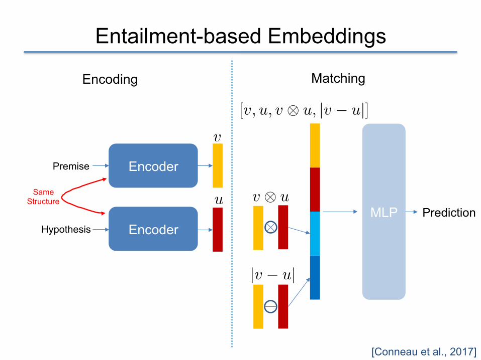
Entailment-based Embeddings
[Conneau et al., 2017]
Encoder
Encoder
MLP Prediction
Premise
Hypothesis
Same Structure
v
u
|v � u|
v ⌦ u
[v, u, v ⌦ u, |v � u|]
Encoding Matching

Entailment-based Embeddings
[Conneau et al., 2017]
Model MR CR SUBJ MPQA SST TREC MRPC SICK-R SICK-E STS14
Unsupervised representation training (unordered sentences)
Unigram-TFIDF 73.7 79.2 90.3 82.4 - 85.0 73.6/81.7 - - .58/.57
ParagraphVec (DBOW) 60.2 66.9 76.3 70.7 - 59.4 72.9/81.1 - - .42/.43
SDAE 74.6 78.0 90.8 86.9 - 78.4 73.7/80.7 - - .37/.38
SIF (GloVe + WR) - - - - 82.2 - - - 84.6 .69/ -
word2vec BOW† 77.7 79.8 90.9 88.3 79.7 83.6 72.5/81.4 0.803 78.7 .65/.64
fastText BOW† 76.5 78.9 91.6 87.4 78.8 81.8 72.4/81.2 0.800 77.9 .63/.62
GloVe BOW† 78.7 78.5 91.6 87.6 79.8 83.6 72.1/80.9 0.800 78.6 .54/.56
GloVe Positional Encoding† 78.3 77.4 91.1 87.1 80.6 83.3 72.5/81.2 0.799 77.9 .51/.54
BiLSTM-Max (untrained)† 77.5 81.3 89.6 88.7 80.7 85.8 73.2/81.6 0.860 83.4 .39/.48
Unsupervised representation training (ordered sentences)
FastSent 70.8 78.4 88.7 80.6 - 76.8 72.2/80.3 - - .63/.64
FastSent+AE 71.8 76.7 88.8 81.5 - 80.4 71.2/79.1 - - .62/.62
SkipThought 76.5 80.1 93.6 87.1 82.0 92.2 73.0/82.0 0.858 82.3 .29/.35
SkipThought-LN 79.4 83.1 93.7 89.3 82.9 88.4 - 0.858 79.5 .44/.45
Supervised representation training
CaptionRep (bow) 61.9 69.3 77.4 70.8 - 72.2 - - - .46/.42
DictRep (bow) 76.7 78.7 90.7 87.2 - 81.0 68.4/76.8 - - .67/.70
NMT En-to-Fr 64.7 70.1 84.9 81.5 - 82.8 - - .43/.42
Paragram-phrase - - - - 79.7 - - 0.849 83.1 .71/ -
BiLSTM-Max (on SST)† (*) 83.7 90.2 89.5 (*) 86.0 72.7/80.9 0.863 83.1 .55/.54
BiLSTM-Max (on SNLI)† 79.9 84.6 92.1 89.8 83.3 88.7 75.1/82.3 0.885 86.3 .68/.65
BiLSTM-Max (on AllNLI)† 81.1 86.3 92.4 90.2 84.6 88.2 76.2/83.1 0.884 86.3 .70/.67
Supervised methods (directly trained for each task – no transfer)
Naive Bayes - SVM 79.4 81.8 93.2 86.3 83.1 - - - - -
AdaSent 83.1 86.3 95.5 93.3 - 92.4 - - - -
TF-KLD - - - - - - 80.4/85.9 - - -
Illinois-LH - - - - - - - - 84.5 -
Dependency Tree-LSTM - - - - - - - 0.868 - -
Table 4: Transfer test results for various architectures trained in different ways. Underlined are best
results for transfer learning approaches, in bold are best results among the models trained in the same
way. † indicates methods that we trained, other transfer models have been extracted from (Hill et al.,
2016). For best published supervised methods (no transfer), we consider AdaSent (Zhao et al., 2015),
TF-KLD (?), Tree-LSTM (Tai et al., 2015) and Illinois-LH system (Lai and Hockenmaier, 2014). (*)
Our model trained on SST obtained 83.4 for MR and 86.0 for SST (MR and SST come from the same
source), which we do not put in the tables for fair comparison with transfer methods.
els (BiLSTM-Max, HConvNet, inner-att), which
demonstrate unequal abilities to incorporate more
information as the size grows. We hypothesize
that such networks are able to incorporate infor-
mation that is not directly relevant to the objective
task (results on SNLI are relatively stable with re-
gard to embedding size) but that can nevertheless
be useful as features for transfer tasks.
5.2 Task transfer
We report in Table 4 transfer tasks results for
different architectures trained in different ways.
We group models by the nature of the data
on which they were trained. The first group
corresponds to models trained with unsuper-
vised unordered sentences. This includes bag-
of-words models such as word2vec-SkipGram,
the Unigram-TFIDF model, the Paragraph Vector
model (Le and Mikolov, 2014), the Sequential De-
noising Auto-Encoder (SDAE) (Hill et al., 2016)
and the SIF model (Arora et al., 2017), all trained
on the Toronto book corpus (?). The second group
consists of models trained with unsupervised or-
dered sentences such as FastSent and SkipThought
(also trained on the Toronto book corpus). We also
include the FastSent variant “FastSent+AE” and
the SkipThought-LN version that uses layer nor-
malization. We report results from models trained
on supervised data in the third group, and also re-
port some results of supervised methods trained
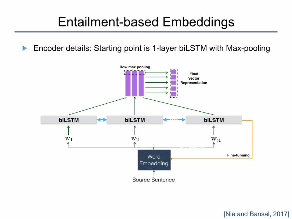
Entailment-based Embeddings
[Nie and Bansal, 2017]
! Encoder details: Starting point is 1-layer biLSTM with Max-pooling
w1 w2
biLSTM biLSTM biLSTM
Row max pooling
FinalVector
Representation
Word Embedding
Source Sentence
Fine-tunning
wn
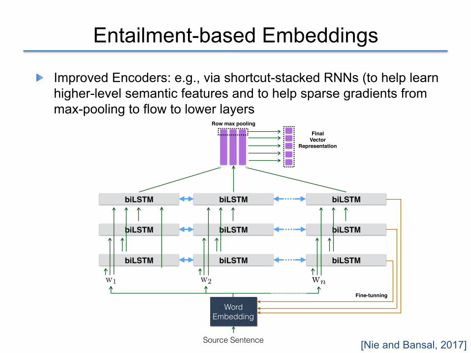
biLSTM
w1 w2
biLSTM biLSTM
biLSTM biLSTM biLSTM
biLSTM biLSTM biLSTM
Row max pooling
FinalVector
Representation
Word Embedding
Source Sentence
Fine-tunning
wn
Entailment-based Embeddings
[Nie and Bansal, 2017]
! Improved Encoders: e.g., via shortcut-stacked RNNs (to help learn higher-level semantic features and to help sparse gradients from max-pooling to flow to lower layers

Entailment-based Embeddings
[Nangia et al., 2017]
! RepEval 2017 Shared Task Results
#Examples #Wds. ‘S’ parsesGenre Train Dev. Test Prem. Prem. Hyp. Agrmt. BiLSTM Acc.
SNLI 550,152 10,000 10,000 14.1 74% 88% 89.0% 81.5%
FICTION 77,348 2,000 2,000 14.4 94% 97% 89.4% 66.8%GOVERNMENT 77,350 2,000 2,000 24.4 90% 97% 87.4% 68.0%SLATE 77,306 2,000 2,000 21.4 94% 98% 87.1% 68.4%TELEPHONE 83,348 2,000 2,000 25.9 71% 97% 88.3% 67.7%TRAVEL 77,350 2,000 2,000 24.9 97% 98% 89.9% 66.8%
9/11 0 2,000 2,000 20.6 98% 99% 90.1% 68.5%FACE-TO-FACE 0 2,000 2,000 18.1 91% 96% 89.5% 67.5%LETTERS 0 2,000 2,000 20.0 95% 98% 90.1% 66.4%OUP 0 2,000 2,000 25.7 96% 98% 88.1% 66.7%VERBATIM 0 2,000 2,000 28.3 93% 97% 87.3% 67.2%
MultiNLI Overall 392,702 20,000 20,000 22.3 91% 98% 88.7% 67.4%
Table 2: Key statistics for the corpus broken down by genre, presented alongside figures from SNLIfor comparison. The first five genres represent the matched section of the development and test sets, andthe remaining five represent the mismatched section. The first three statistics shown are the number ofexamples in each genre. #Wds. Prem. is the mean token count among premise sentences. ‘S’ parses isthe percentage of premises or hypotheses which the Stanford Parser labeled as full sentences rather thanfragments. Agrmt. is the percent of individual annotator labels that match the assigned gold label usedin evaluation. BiLSTM Acc. gives the test accuracy on the full test set for the BiLSTM baseline modeltrained on MultiNLI and SNLI.
Team Name Authors Matched Mismatched Model Details
alpha (ensemble) Chen et al. 74.9% 74.9% STACK, CHAR, ATTN., POOL, PRODDIFFYixinNie-UNC-NLP Nie and Bansal 74.5% 73.5% STACK, POOL, PRODDIFF, SNLIalpha Chen et al. 73.5% 73.6% STACK, CHAR, ATTN, POOL, PRODDIFFRivercorners (ensemble) Balazs et al. 72.2% 72.8% ATTN, POOL, PRODDIFF, SNLIRivercorners Balazs et al. 72.1% 72.1% ATTN, POOL, PRODDIFF, SNLILCT-MALTA Vu et al. 70.7% 70.8% CHAR, ENHEMB, PRODDIFF, POOLTALP-UPC Yang et al. 67.9% 68.2% CHAR, ATTN, SNLIBiLSTM baseline Williams et al. 67.0% 67.6% POOL, PRODDIFF, SNLI
Table 3: RepEval 2017 shared task competition results. The Model Details column lists some of the keystrategies used in each system, using keywords: STACK: use of multilayer bidirectional RNNs, CHAR:character-level embeddings, ENHEMB: embeddings enhanced with auxiliary features, POOL: max ormean pooling over RNN states, ATTN: intra-sentence attention, PRODDIFF: elementwise sentence prod-uct and difference features in the final entailment classifier, SNLI: use of the SNLI training set.
veys the key differences between systems, and theModel Details column in Table 3 serves as a sum-mary reference for these differences.
Depth Chen et al. and Nie and Bansal use three-layer bidirectional RNNs, while others only usedsingle-layer RNNs. This likely contributes signif-icantly to their good performance, as it is the mostprominent feature shared only by these two topsystems. They both use shortcut connections be-tween recurrent layers to ease gradient flow, andNie and Bansal find in an ablation study that usingshortcut connections improves their performanceby over 1% on both development sets.
Embeddings Systems vary reasonably widelyin their approach to input encoding. Yanget al. and Chen et al. use a combination of GloVeembeddings (Pennington et al., 2014, not finetuned) and character-level convolutional neuralnetworks (Kim et al., 2016) to extract represen-tations of words. Balazs et al. also use pre-trainedGloVe embeddings without fine tuning, but report(contra Chen et al.) that an added character-levelfeature extractor does not improve performance.
Vu et al. use pre-trained GloVe word embed-dings augmented with additional feature vectors.They create embeddings for part-of-speech (POS),character level information, and the dependencyrelation between a word and its parent, and con-
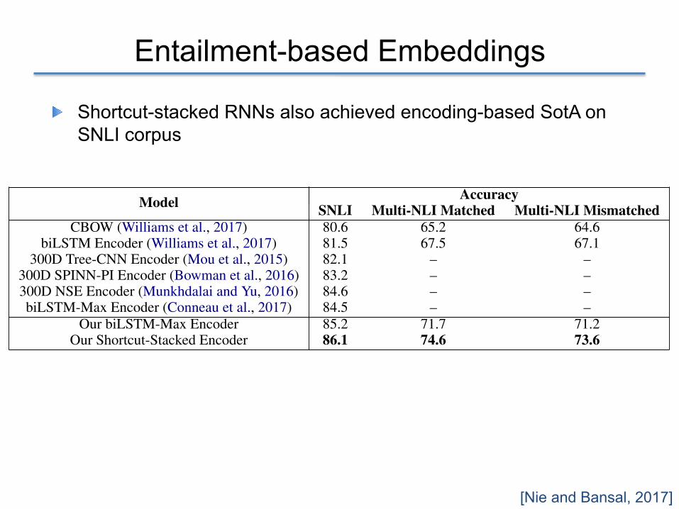
Entailment-based Embeddings
[Nie and Bansal, 2017]
! Shortcut-stacked RNNs also achieved encoding-based SotA on SNLI corpus
Model
Accuracy
SNLI Multi-NLI Matched Multi-NLI Mismatched
CBOW (Williams et al., 2017) 80.6 65.2 64.6biLSTM Encoder (Williams et al., 2017) 81.5 67.5 67.1
300D Tree-CNN Encoder (Mou et al., 2015) 82.1 – –300D SPINN-PI Encoder (Bowman et al., 2016) 83.2 – –300D NSE Encoder (Munkhdalai and Yu, 2016) 84.6 – –biLSTM-Max Encoder (Conneau et al., 2017) 84.5 – –
Our biLSTM-Max Encoder 85.2 71.7 71.2Our Shortcut-Stacked Encoder 86.1 74.6 73.6
Table 5: Final Test Results on SNLI and Multi-NLI datasets.
mization with 32 batch size. The starting learningrate is 0.0002 with half decay every two epochs.The number of hidden units for MLP in classifieris 1600. Dropout layer is also applied on the out-put of each layer of MLP, with dropout rate set to0.1. We used pre-trained 300D Glove 840B vec-tors (Pennington et al., 2014) to initialize the wordembeddings. Tuning decisions for word embed-ding training strategy, the hyperparameters of di-mension and number of layers for biLSTM, andthe activation type and number of layers for MLP,are all explained in Section 4.
4 Results and Analysis
4.1 Ablation Analysis Results
We now investigate the effectiveness of each of theenhancement components in our overall model.These ablation results are shown in Tables 1, 2, 3and 4, all based on the Multi-NLI developmentsets. Finally, Table 5 shows results for differentencoders on SNLI and Multi-NLI test sets.
First, Table 1 shows the performance changesfor different number of biLSTM layers and theirvarying dimension size. The dimension size ofa biLSTM layer is referring to the dimension ofthe hidden state for both the forward and back-ward LSTM-RNNs. As shown, each added layermodel improves the accuracy and we achieve asubstantial improvement in accuracy (around 2%)on both matched and mismatched settings, com-pared to the single-layer biLSTM in Conneau et al.(2017). We only experimented with up to 3 lay-ers with 512, 1024, 2048 dimensions each, so themodel still has potential to improve the result fur-ther with a larger dimension and more layers.
Next, in Table 2, we show that the shortcutconnections among the biLSTM layers is alsoan important contributor to accuracy improve-ment (around 1.5% on top of the full 3-layeredstacked-RNN model). This demonstrates that sim-ply stacking the biLSTM layers is not sufficient
to handle a complex task like Multi-NLI and it issignificantly better to have the higher layer con-nected to both the output and the original input ofall the previous layers (note that Table 1 results arebased on multi-layered models with shortcut con-nections).
Next, in Table 3, we show that fine-tuning theword embeddings also improves results, again forboth the in-domain task and cross-domain tasks(the ablation results are based on a smaller modelwith a 128+256 2-layer biLSTM). Hence, all ourmodels were trained with word embeddings beingfine-tuned. The last ablation in Table 4 shows thata classifier with two layers of relu is preferablethan other options. Thus, we use that setting forour strongest encoder.
4.2 Multi-NLI and SNLI Test Results
Finally, in Table 5, we report the test resultsfor MNLI and SNLI. First for Multi-NLI, weimprove substantially over the CBOW and biL-STM Encoder baselines reported in the dataset pa-per (Williams et al., 2017). We also show thatour final shortcut-based stacked encoder achievesaround 3% improvement as compared to the 1-layer biLSTM-Max Encoder in the second lastrow (using the exact same classifier and optimizersettings). Our shortcut-encoder was also the topsinge-model (non-ensemble) result on the EMNLPRepEval Shared Task leaderboard.
Next, for SNLI, we compare our shortcut-stacked encoder with the current state-of-the-artencoders from the SNLI leaderboard (https://nlp.stanford.edu/projects/snli/).We also compare to the recent biLSTM-MaxEncoder of Conneau et al. (2017), which servedas our model’s 1-layer starting point.1 The resultsindicate that ‘Our Shortcut-Stacked Encoder’ sur-
1Note that the ‘Our biLSTM-Max Encoder’ results in thesecond-last row are obtained using our reimplementation ofthe Conneau et al. (2017) model; our version is 0.7% better,likely due to our classifier and optimizer settings.
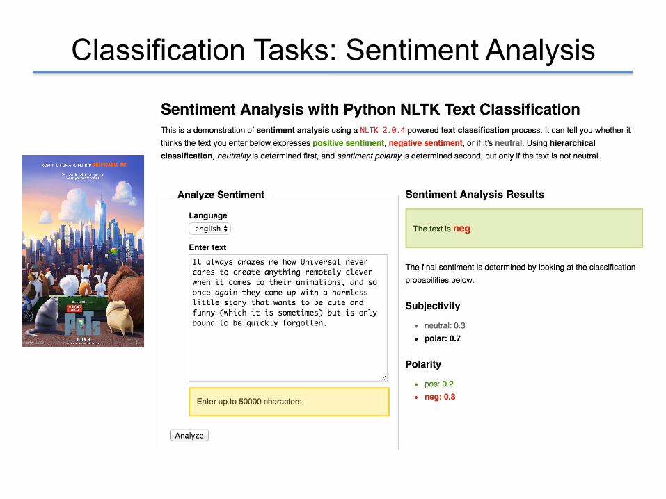
Classification Tasks: Sentiment Analysis

Sentiment Analysis
! Earlier methods used bag of words, e.g., lexicons of positive and negative words and phrases
! Cannot distinguish tricky cases like:
+ white blood cells destroying an infection− an infection destroying white blood cells+ There are slow and repetitive parts but it has just enough spice to keep it interesting.− Stealing Harvard doesn’t care about cleverness, wit or any other kind of intelligent humor.

Sentiment Analysis
! Even simpler issues like negation hard to understand
! Socher et al., 2013b present new compositional training data and new composition model
Recursive Deep Models for Semantic CompositionalityOver a Sentiment Treebank
Richard Socher, Alex Perelygin, Jean Y. Wu, Jason Chuang,Christopher D. Manning, Andrew Y. Ng and Christopher Potts
Stanford University, Stanford, CA 94305, [email protected],{aperelyg,jcchuang,ang}@cs.stanford.edu
{jeaneis,manning,cgpotts}@stanford.edu
Abstract
Semantic word spaces have been very use-ful but cannot express the meaning of longerphrases in a principled way. Further progresstowards understanding compositionality intasks such as sentiment detection requiresricher supervised training and evaluation re-sources and more powerful models of com-position. To remedy this, we introduce aSentiment Treebank. It includes fine grainedsentiment labels for 215,154 phrases in theparse trees of 11,855 sentences and presentsnew challenges for sentiment composition-ality. To address them, we introduce theRecursive Neural Tensor Network. Whentrained on the new treebank, this model out-performs all previous methods on several met-rics. It pushes the state of the art in singlesentence positive/negative classification from80% up to 85.4%. The accuracy of predictingfine-grained sentiment labels for all phrasesreaches 80.7%, an improvement of 9.7% overbag of features baselines. Lastly, it is the onlymodel that can accurately capture the effectsof negation and its scope at various tree levelsfor both positive and negative phrases.
1 Introduction
Semantic vector spaces for single words have beenwidely used as features (Turney and Pantel, 2010).Because they cannot capture the meaning of longerphrases properly, compositionality in semantic vec-tor spaces has recently received a lot of attention(Mitchell and Lapata, 2010; Socher et al., 2010;Zanzotto et al., 2010; Yessenalina and Cardie, 2011;Socher et al., 2012; Grefenstette et al., 2013). How-ever, progress is held back by the current lack oflarge and labeled compositionality resources and
–
0
0
This
0
film
–
–
–
0
does
0
n’t
0
+
care
+
0
about
+
+
+
+
+
cleverness
0
,
0
wit
0
or
+
0
0
any
0
0
other
+
kind
+
0
of
+
+
intelligent
+ +
humor
0
.
Figure 1: Example of the Recursive Neural Tensor Net-work accurately predicting 5 sentiment classes, very neg-ative to very positive (– –, –, 0, +, + +), at every node of aparse tree and capturing the negation and its scope in thissentence.
models to accurately capture the underlying phe-nomena presented in such data. To address this need,we introduce the Stanford Sentiment Treebank anda powerful Recursive Neural Tensor Network thatcan accurately predict the compositional semanticeffects present in this new corpus.
The Stanford Sentiment Treebank is the first cor-pus with fully labeled parse trees that allows for acomplete analysis of the compositional effects ofsentiment in language. The corpus is based onthe dataset introduced by Pang and Lee (2005) andconsists of 11,855 single sentences extracted frommovie reviews. It was parsed with the Stanfordparser (Klein and Manning, 2003) and includes atotal of 215,154 unique phrases from those parsetrees, each annotated by 3 human judges. This newdataset allows us to analyze the intricacies of senti-ment and to capture complex linguistic phenomena.Fig. 1 shows one of the many examples with clearcompositional structure. The granularity and size of
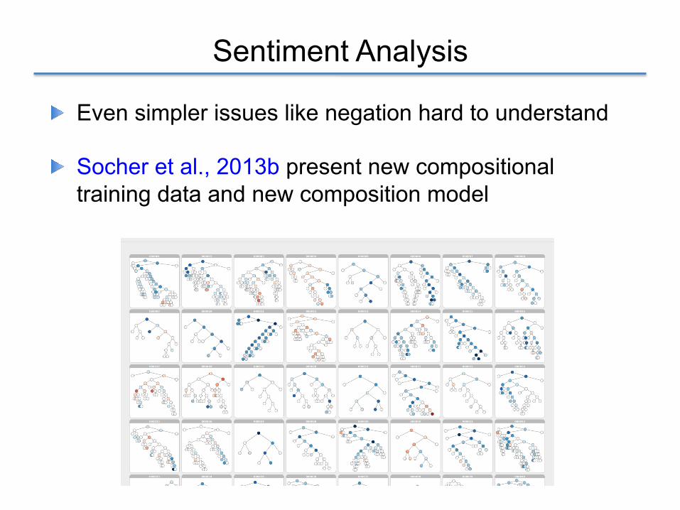
Sentiment Analysis
! Even simpler issues like negation hard to understand
! Socher et al., 2013b present new compositional training data and new composition model 1.NewSentimentTreebank

Sentiment Analysis
! Sentiment Compositionality: 1.NewSentimentTreebank
• Parsetreesof11,855sentences• 215,154phraseswithlabels• Allowstrainingandevaluating
withcompositionalinformation

Sentiment Analysis
! Better Models: Recursive Neural Tensor Network (RNTN)
RecursiveNeuralTensorNetworkRecursiveDeepModels forSemanticCompositionalityOveraSentimentTreebankSocheretal.2013

Sentiment Analysis
! Better Models: Tree-based LSTM-RNNs
TreeLSTMs
• Wecanusethoseideasingrammaticaltreestructures!
• Paper:Taietal.2015:ImprovedSemanticRepresentationsFromTree-StructuredLongShort-TermMemoryNetworks
• Idea:Sumthechildvectorsinatreestructure
• Eachchildhasitsownforgetgate
• Samesoftmax onh
5/5/16RichardSocherLecture1,Slide 40

Sentiment Compositionality
! Demos: h#p://nlp.stanford.edu:8080/sen7ment/rntnDemo.html [Yessenalina and Cardie, 2011; Socher et al., 2013b]
ResultsonStanfordSentimentTreebank
Method Fine-grained Binary
RAE (Socher et al., 2013) 43.2 82.4MV-RNN (Socher et al., 2013) 44.4 82.9RNTN (Socher et al., 2013) 45.7 85.4DCNN (Blunsom et al., 2014) 48.5 86.8Paragraph-Vec (Le and Mikolov, 2014) 48.7 87.8CNN-non-static (Kim, 2014) 48.0 87.2CNN-multichannel (Kim, 2014) 47.4 88.1DRNN (Irsoy and Cardie, 2014) 49.8 86.6
LSTM 45.8 86.7Bidirectional LSTM 49.1 86.82-layer LSTM 47.5 85.52-layer Bidirectional LSTM 46.2 84.8
Constituency Tree LSTM (no tuning) 46.7 86.6Constituency Tree LSTM 50.6 86.9
Table 2: Test set accuracies on the Stanford Senti-ment Treebank. Fine-grained: 5-class sentimentclassification. Binary: positive/negative senti-ment classification. We give results for Tree-LSTM models with and without fine-tuning ofword representations.
Sec. 4.2. For the similarity prediction network(Eqs. 15) we use a hidden layer of size 50. Wecompare two Tree-LSTM architectures for com-posing sentence representations: the Child-SumTree-LSTM architecture (Sec. 3.1) on dependencytrees (Chen and Manning, 2014) and the BinaryTree-LSTM (Sec. 3.2) on binarized constituencytrees (Klein and Manning, 2003).
5.3 Hyperparameters and Training DetailsThe hyperparameters for our models were tunedon the development set for each task.
We initialized our word representations usingpublicly available 300-dimensional Glove vectors(Pennington et al., 2014). For the sentiment classi-fication task, word representations were fine-tunedduring training with a learning rate of 0.1; no fine-tuning was performed for the semantic relatednesstask.
Our models were trained using AdaGrad (Duchiet al., 2011) with a learning rate of 0.05 and aminibatch size of 25. The model parameters wereregularized with a per-minibatch L2 regularizationstrength of 10�4. The sentiment classifier was ad-ditionally regularized using dropout (Hinton et al.,2012).
6 Results
6.1 Sentiment ClassificationOur results are summarized in Table 2. As was thecase with the convolutional neural network model
Method r ⇢ MSE
Mean vectors 0.8046 0.7294 0.3595DT-RNN (Socher et al., 2014) 0.7863 0.7305 0.3983SDT-RNN (Socher et al., 2014) 0.7886 0.7280 0.3859
Illinois-LH (Lai and Hockenmaier, 2014) 0.7993 0.7538 0.3692UNAL-NLP (Jimenez et al., 2014) 0.8070 0.7489 0.3550Meaning Factory (Bjerva et al., 2014) 0.8268 0.7721 0.3224ECNU (Zhao et al., 2014) 0.8414 – –
LSTM 0.8477 0.7921 0.2949Bidirectional LSTM 0.8522 0.7952 0.28502-layer LSTM 0.8411 0.7849 0.29802-layer Bidirectional LSTM 0.8488 0.7926 0.2893
Constituency Tree LSTM 0.8491 0.7873 0.2852Dependency Tree LSTM 0.8627 0.8032 0.2635
Table 3: Test set results on the SICK semanticrelatedness subtask. The evaluation metrics arePearson’s r, Spearman’s ⇢, and mean squared er-ror. Results are grouped as follows: (1) Our ownbaselines; (2) SemEval 2014 submissions; (3) Se-quential LSTM variants.
described by Kim (2014), we found that tuningword representations yielded a significant boost inperformance on the fine-grained classification sub-task, in contrast to the minor gains observed on thebinary classification subtask. This suggests thatfine-tuning helps distinguish positive/negative vs.neutral, strongly positive vs. positive, and stronglynegative vs. negative, as opposed to positive vs.negative in the binary case.
The Bidirectional LSTM significantly outper-formed the standard LSTM on the fine-grainedsubtask. Note that this result is achieved with-out introducing any additional parameters in theLSTM transition function since the forward andbackward parameters are shared. This indicatesthat sentence length becomes a limiting factorfor the (unidirectional) LSTM on the fine-grainedsubtask. Somewhat surprisingly, we do not ob-serve a corresponding improvement on the binarysubtask (indeed, we achieve similar results on allour single-layer LSTM models). We conjecturethat the state that needs to be retained by the net-work in order to make a correct binary predictionis easily preserved by both the LSTM and Bidi-rectional LSTM models, whereas the fine-grainedcase requires more complex interactions betweenthe input word representations and the hidden stateof the LSTM unit.
The Tree-LSTM over constituency trees outper-forms existing systems on the fine-grained classi-fication subtask.
5/5/16RichardSocherLecture1,Slide 41
ofwordvectors

Other Classification Tasks
! Sentence similarity
! Entailment classification
! Spam detection
! Document topic classification
! Others: humor, rumor, sarcasm detection, etc.
SemEval has great new tasks every year with novel datasets in many cases! Some recent years: http://alt.qcri.org/semeval2017/index.php?id=tasks http://alt.qcri.org/semeval2016/index.php?id=tasks http://alt.qcri.org/semeval2015/index.php?id=tasks


![index []...p 104—109 comp. 190 p 110—115 comp. 191 p 116—121 comp. 192 p 122—127 comp. 193 p 128—133 comp. 194 p 134—139 comp. 195 p 140—147 comp. 196 p 148—153 comp.](https://static.fdocuments.in/doc/165x107/5f95526362174b59db2f2d15/index-p-104a109-comp-190-p-110a115-comp-191-p-116a121-comp-192.jpg)


![COMP 790.139 (Fall 2017) Natural Language Processingmbansal/teaching/slidesFall17/nlp_comp790_fall2… · Figure 12.6 All the ways to fill the [i, j] ... The standard techniques](https://static.fdocuments.in/doc/165x107/5f7ce82a6c0aa3387d38b862/comp-790139-fall-2017-natural-language-mbansalteachingslidesfall17nlpcomp790fall2.jpg)