Community Ecology BDC321 Mark J Gibbons, Room 4.102, BCB Department, UWC Tel: 021 959 2475. Email:...
18
Community Ecology BDC321 Mark J Gibbons, Room 4.102, BCB Department, UWC Tel: 021 959 2475. Email: [email protected] Image acknowledgements – http://www.google.com
-
Upload
brook-bates -
Category
Documents
-
view
218 -
download
1
Transcript of Community Ecology BDC321 Mark J Gibbons, Room 4.102, BCB Department, UWC Tel: 021 959 2475. Email:...

Community Ecology
BDC321
Mark J Gibbons, Room 4.102, BCB Department, UWC
Tel: 021 959 2475. Email: [email protected]
Image acknowledgements – http://www.google.com

Measures of Community Diversity
Species Richness - S
Description of Communities
A B
6565TOTAL
12LIGHT BLUE
23APPLE GREEN
79BLACK
24DARK BLUE
45LIGHT GREEN
36ORANGE
24YELLOW
314LILAC
4118RED
BACOLOUR
Same Number Species – 9
Same Number individuals - 65
Different Distribution of individuals amongst species
GuildTaxocene

Determining Species Richness
Species DensityNumber of Species Observed
Total Number of Individuals Counted
Botanists
Numerical Species Richness
Sample-based
Samples taken: all individuals within identified & counted
Individual-based
Individuals sampled sequentially
Focus of Community Studies
PROBLEM: Number of species reflects number of samples
or individuals

COMMUNITIES
vs
SAMPLES
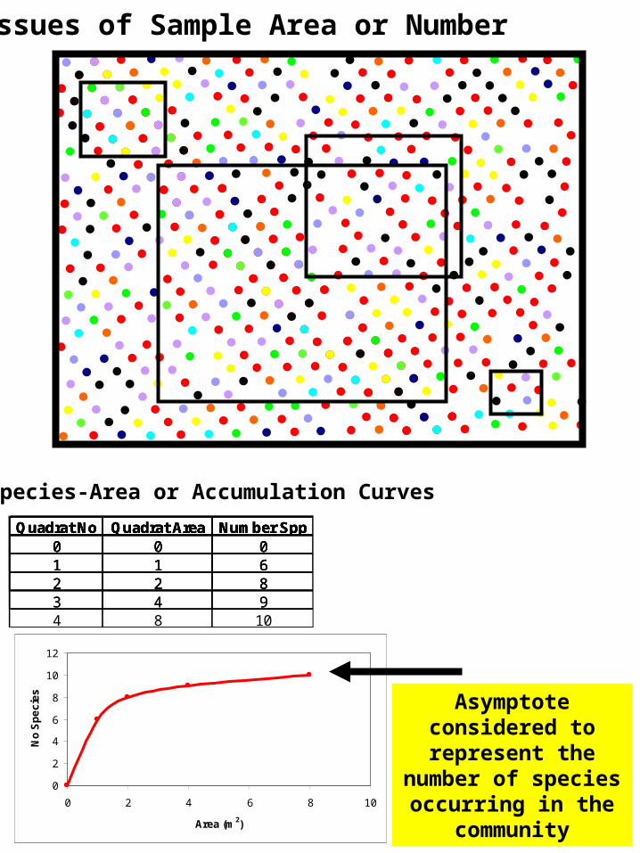
Issues of Sample Area or Number
Species-Area or Accumulation Curves
0
2
4
6
8
10
12
0 2 4 6 8 10
Area (m2)
No
Sp
ec
ies
Asymptote considered to
represent the number of species occurring
in the community
Quadrat No Quadrat Area Number Spp Number Unique Spp Cumulative No Spp0 0 0 0 01 1 6 6 62 2 8 2 83 4 9 1 94 8 10 1 10
Quadrat No Quadrat Area Number Spp Number Unique Spp Cumulative No Spp0 0 0 0 01 1 6 6 62 2 8 2 83 4 9 1 94 8 10 1 10
Quadrat No Quadrat Area Number Spp Number Unique Spp Cumulative No Spp0 0 0 0 01 1 6 6 62 2 8 2 83 4 9 1 94 8 10 1 10
Quadrat No Quadrat Area Number Spp Number Unique Spp Cumulative No Spp0 0 0 0 01 1 6 6 62 2 8 2 83 4 9 1 94 8 10 1 10

1 2 3 4 5 6 7 8 9 10 11Black 1 3 2 2 1 1Red 1 3 3 3 1 1 1 1 1 3
Yellow 1 3 1 1 1 1 1Green 1 1Green 2 1Blue 1 1 1Blue 2 2 1 1 1 1 1 1
Purple 1 2 1 1 1Purple 2 1 1Orange 1 2 1 1 1 1
Total No spp 3 4 2 3 3 4 5 7 6 5 4Total No Individuals 4 8 4 7 6 5 5 7 6 5 6
No Unique Spp 3 2 0 1 0 0 0 1 1 1 0Cumulative No Spp 3 5 5 6 6 6 6 7 8 9 9
Cumulative Area 1 2 3 4 5 6 7 8 9 10 11
Quadrat NoSpecies
0123456789
10
1 2 3 4 5 6 7 8 9 10 11
Area
No
Sp
ec
ies

Species Quadrat No7 8 9 10 11 1 2 3 4 5 6
Black 1 1 1 3 2 2Red 1 1 1 1 3 1 3 3 3 1
Yellow 1 1 1 1 1 3 1Green 1 1Green 2 1Blue 1 1 1Blue 2 1 1 1 1 2 1 1
Purple 1 1 1 1 2Purple 2 1 1Orange 1 1 1 1 2 1
Total No spp 5 7 6 5 4 3 4 2 3 3 4Total No Individuals 5 7 6 5 6 4 8 4 7 6 5
No Unique Spp 5 3 1 0 0 0 0 0 0 0 0Cumulative No Spp 5 8 9 9 9 9 9 9 9 9 9
Cumulative Area 1 2 3 4 5 6 7 8 9 10 11
0
2
4
6
8
10
1 2 3 4 5 6 7 8 9 10 11
Area
No
Sp
ecie
s

Randomised 999 times
Rarefaction Curves
The absolute number of species likely to be found in the pool is obtained when the curve flattens out
WHEN IDENTIFYING or COMPARING COMMUNITIES, ARE YOU INTERESTED IN
ESTIMATING ABSOLUTE RICHNESS?
DEPENDS ON THE QUESTION BEING ASKED
There are a number of ways of determining this:

Effort (area or number of samples or individuals) is important
STANDARDIZE
a priori
HOW?

Species Diversity Indices
Heterogeneity Measures
Shannon Index (H’ )
A B C D E F G HI 0 0 0 0 0 2 5 8II 9 8 1 6 8 2 7 5III 1 3 0 3 9 7 0 0IV 2 2 1 5 7 8 3 8V 2 4 3 2 3 7 6 3VI 3 8 9 10 1 3 4 1VII 2 0 0 10 0 2 9 5VIII 7 0 3 6 0 1 2 7IX 4 2 10 7 0 8 3 6X 0 7 6 4 2 3 2 1XI 2 4 3 8 6 5 1 5XII 9 2 1 1 1 6 8 8XIII 4 9 8 2 4 10 0 4XIV 5 1 10 5 3 9 7 8
50 50 55 69 44 73 57 69TOTAL
SAMPLE
SP
EC
IES
A B C D E F G HI 0.00 0.00 0.00 0.00 0.00 0.03 0.09 0.12II 0.18 0.16 0.02 0.09 0.18 0.03 0.12 0.07III 0.02 0.06 0.00 0.04 0.20 0.10 0.00 0.00IV 0.04 0.04 0.02 0.07 0.16 0.11 0.05 0.12V 0.04 0.08 0.05 0.03 0.07 0.10 0.11 0.04VI 0.06 0.16 0.16 0.14 0.02 0.04 0.07 0.01VII 0.04 0.00 0.00 0.14 0.00 0.03 0.16 0.07VIII 0.14 0.00 0.05 0.09 0.00 0.01 0.04 0.10IX 0.08 0.04 0.18 0.10 0.00 0.11 0.05 0.09X 0.00 0.14 0.11 0.06 0.05 0.04 0.04 0.01XI 0.04 0.08 0.05 0.12 0.14 0.07 0.02 0.07XII 0.18 0.04 0.02 0.01 0.02 0.08 0.14 0.12XIII 0.08 0.18 0.15 0.03 0.09 0.14 0.00 0.06XIV 0.10 0.02 0.18 0.07 0.07 0.12 0.12 0.12
1 1 1 1 1 1 1 1
SAMPLE
SP
EC
IES
TOTAL
H’ = - pi ln(pi)∑pi = Proportion of the ith species
Varies between 1.5 and 4.
Should ONLY really be used for datasets where absolute richness known – otherwise Brillouin Index
Sensitive to the abundance of rare species

Brillouin Index
H1
Nln N!( )
n1! n2! n3! n4! ......=
n1 = Number of individuals of species 1n2 = Number of individuals of species 2
N = total number of individuals in the entire collection
^H can only use count data
Best used where data not random
Sensitive to the abundance of rare species

Simpson’s Index D = pi2∑
pi = Proportion of the ith species
This Index actually determines the probability of two organisms at random that are the same species
[ ]D = ^ ∑ ni (ni – 1)
N (N – 1)
ni = Number of individuals of species i in the sample
N = Total number of individuals in the sample
s = Number of species in the sample
i = 1
s
D can use biomass, cover, productivity & count data.
^D can only use count data.
Sensitive to the abundance of common species
Species Evenness Measures
1 - DSimpson’s Index of Diversity
The probability that two organisms drawn at random are different species
1D
Strictly speaking, D can only be used for an infinite population - Estimator

Evenness Diversity
Maximum Diversity
H’
Hmax
Shannon (J)
Hmax = ln(S) S = Number of Species
Simpson’s 1 / D
SE1/D =

Putting Confidence Intervals around Estimates
Jackknifing – the generation of pseudo-means
Species 1 2 3 4 5 6 7 8 9 10 11 12 13 14 15 16
1 0 0 0 0 0 0 0 0 0 0 12 0 32 2 0 0
2 0 0 0 0 0 0 0 0 0 0 0 1 0 0 0 0
3 1 0 0 0 0 2 0 0 0 2 0 1 0 2 0 0
4 0 1 0 0 0 0 0 0 0 0 0 1 1 0 0 0
5 2 0 0 0 0 1 0 0 0 2 0 0 0 0 1 2
6 0 0 0 2 0 0 0 0 0 0 0 0 0 1 0 1
7 6 0 4 3 4 3 2 1 0 1 5 11 0 3 9 2
8 1 1 0 3 0 2 0 0 0 1 0 5 0 0 3 0
9 0 0 0 0 0 1 0 1 0 0 0 0 0 0 0 0
10 0 0 0 0 0 1 0 0 0 0 0 1 0 0 0 0
11 0 1 0 0 0 4 1 0 0 0 0 2 0 1 0 0
12 1 0 0 0 4 0 0 0 0 1 0 9 0 0 1 0
13 1 0 0 0 0 0 0 0 0 0 0 0 0 0 0 1
14 0 0 0 0 0 1 0 0 0 0 0 0 1 0 0 0
15 0 0 0 2 1 1 0 0 0 0 0 0 0 0 0 0
16 1 0 0 0 0 0 0 0 0 0 0 0 0 0 0 0
17 0 0 0 0 0 1 0 0 1 0 0 0 0 0 0 0
18 0 0 0 0 0 0 0 0 0 0 0 0 0 0 1 0
19 0 0 0 0 0 0 0 0 0 2 0 1 1 0 1 1
20 0 0 0 0 0 0 0 0 0 0 0 0 0 0 0 1
TOTAL 13 3 4 10 9 17 3 2 1 9 17 32 35 9 16 8
SAMPLE
[ ]D = ^ ∑ ni (ni – 1)
N (N – 1)i = 1
s
Simpson’s Index of Diversity
1D
Example using:
Numbers of beetles in 16 hedgerow samples
Species 1 2 3 4 5 6 7 8 9 10 11 12 13 14 15 16
1 0 0 0 0 0 0 0 0 0 0 12 0 32 2 0 0 46
2 0 0 0 0 0 0 0 0 0 0 0 1 0 0 0 0 1
3 1 0 0 0 0 2 0 0 0 2 0 1 0 2 0 0 8
4 0 1 0 0 0 0 0 0 0 0 0 1 1 0 0 0 3
5 2 0 0 0 0 1 0 0 0 2 0 0 0 0 1 2 8
6 0 0 0 2 0 0 0 0 0 0 0 0 0 1 0 1 4
7 6 0 4 3 4 3 2 1 0 1 5 11 0 3 9 2 54
8 1 1 0 3 0 2 0 0 0 1 0 5 0 0 3 0 16
9 0 0 0 0 0 1 0 1 0 0 0 0 0 0 0 0 2
10 0 0 0 0 0 1 0 0 0 0 0 1 0 0 0 0 2
11 0 1 0 0 0 4 1 0 0 0 0 2 0 1 0 0 9
12 1 0 0 0 4 0 0 0 0 1 0 9 0 0 1 0 16
13 1 0 0 0 0 0 0 0 0 0 0 0 0 0 0 1 2
14 0 0 0 0 0 1 0 0 0 0 0 0 1 0 0 0 2
15 0 0 0 2 1 1 0 0 0 0 0 0 0 0 0 0 4
16 1 0 0 0 0 0 0 0 0 0 0 0 0 0 0 0 1
17 0 0 0 0 0 1 0 0 1 0 0 0 0 0 0 0 2
18 0 0 0 0 0 0 0 0 0 0 0 0 0 0 1 0 1
19 0 0 0 0 0 0 0 0 0 2 0 1 1 0 1 1 6
20 0 0 0 0 0 0 0 0 0 0 0 0 0 0 0 1 1
TOTAL 13 3 4 10 9 17 3 2 1 9 17 32 35 9 16 8 188
SAMPLEn
Species 1 2 3 4 5 6 7 8 9 10 11 12 13 14 15 16
1 0 0 0 0 0 0 0 0 0 0 12 0 32 2 0 0 46 45 2070 0.0589
2 0 0 0 0 0 0 0 0 0 0 0 1 0 0 0 0 1 0 0 0.0000
3 1 0 0 0 0 2 0 0 0 2 0 1 0 2 0 0 8 7 56 0.0016
4 0 1 0 0 0 0 0 0 0 0 0 1 1 0 0 0 3 2 6 0.0002
5 2 0 0 0 0 1 0 0 0 2 0 0 0 0 1 2 8 7 56 0.0016
6 0 0 0 2 0 0 0 0 0 0 0 0 0 1 0 1 4 3 12 0.0003
7 6 0 4 3 4 3 2 1 0 1 5 11 0 3 9 2 54 53 2862 0.0814
8 1 1 0 3 0 2 0 0 0 1 0 5 0 0 3 0 16 15 240 0.0068
9 0 0 0 0 0 1 0 1 0 0 0 0 0 0 0 0 2 1 2 0.0001
10 0 0 0 0 0 1 0 0 0 0 0 1 0 0 0 0 2 1 2 0.0001
11 0 1 0 0 0 4 1 0 0 0 0 2 0 1 0 0 9 8 72 0.0020
12 1 0 0 0 4 0 0 0 0 1 0 9 0 0 1 0 16 15 240 0.0068
13 1 0 0 0 0 0 0 0 0 0 0 0 0 0 0 1 2 1 2 0.0001
14 0 0 0 0 0 1 0 0 0 0 0 0 1 0 0 0 2 1 2 0.0001
15 0 0 0 2 1 1 0 0 0 0 0 0 0 0 0 0 4 3 12 0.0003
16 1 0 0 0 0 0 0 0 0 0 0 0 0 0 0 0 1 0 0 0.0000
17 0 0 0 0 0 1 0 0 1 0 0 0 0 0 0 0 2 1 2 0.0001
18 0 0 0 0 0 0 0 0 0 0 0 0 0 0 1 0 1 0 0 0.0000
19 0 0 0 0 0 0 0 0 0 2 0 1 1 0 1 1 6 5 30 0.0009
20 0 0 0 0 0 0 0 0 0 0 0 0 0 0 0 1 1 0 0 0.0000
TOTAL 13 3 4 10 9 17 3 2 1 9 17 32 35 9 16 8 188 0.1612
SAMPLEn n-1 n.(n-1) n.(n-1)/N.(N-1)
DSt = 0.1612 1 / DSt = 6.20473

Repeat calculations n times, where n = number of samples, missing out each sample i in turn
Species 1 2 3 4 5 6 7 8 9 10 11 12 13 14 15 16
1 0 0 0 0 0 0 0 0 0 12 0 32 2 0 0 46 45 2070 0.0680
2 0 0 0 0 0 0 0 0 0 0 1 0 0 0 0 1 0 0 0.0000
3 0 0 0 0 2 0 0 0 2 0 1 0 2 0 0 7 6 42 0.0014
4 1 0 0 0 0 0 0 0 0 0 1 1 0 0 0 3 2 6 0.0002
5 0 0 0 0 1 0 0 0 2 0 0 0 0 1 2 6 5 30 0.0010
6 0 0 2 0 0 0 0 0 0 0 0 0 1 0 1 4 3 12 0.0004
7 0 4 3 4 3 2 1 0 1 5 11 0 3 9 2 48 47 2256 0.0741
8 1 0 3 0 2 0 0 0 1 0 5 0 0 3 0 15 14 210 0.0069
9 0 0 0 0 1 0 1 0 0 0 0 0 0 0 0 2 1 2 0.0001
10 0 0 0 0 1 0 0 0 0 0 1 0 0 0 0 2 1 2 0.0001
11 1 0 0 0 4 1 0 0 0 0 2 0 1 0 0 9 8 72 0.0024
12 0 0 0 4 0 0 0 0 1 0 9 0 0 1 0 15 14 210 0.0069
13 0 0 0 0 0 0 0 0 0 0 0 0 0 0 1 1 0 0 0.0000
14 0 0 0 0 1 0 0 0 0 0 0 1 0 0 0 2 1 2 0.0001
15 0 0 2 1 1 0 0 0 0 0 0 0 0 0 0 4 3 12 0.0004
16 0 0 0 0 0 0 0 0 0 0 0 0 0 0 0 0 -1 0 0.0000
17 0 0 0 0 1 0 0 1 0 0 0 0 0 0 0 2 1 2 0.0001
18 0 0 0 0 0 0 0 0 0 0 0 0 0 1 0 1 0 0 0.0000
19 0 0 0 0 0 0 0 0 2 0 1 1 0 1 1 6 5 30 0.0010
20 0 0 0 0 0 0 0 0 0 0 0 0 0 0 1 1 0 0 0.0000
TOTAL 0 3 4 10 9 17 3 2 1 9 17 32 35 9 16 8 175 0.1628
SAMPLEn n-1 n.(n-1) n.(n-1)/N.(N-1)
Record D(St-1) value – calculate reciprocal

D(St-1) 1 / D(st-1)
1 0.1628 6.14252 0.165 6.06063 0.156 6.41034 0.1666 6.00245 0.1613 6.19966 0.1785 5.60227 0.1598 6.25788 0.1615 6.19209 0.1628 6.1425
10 0.1704 5.868511 0.1448 6.906112 0.1746 5.727413 0.1618 6.180514 0.1609 6.215015 0.158 6.329116 0.168 5.9524
SA
MP
LE
Ф = n . 1 / D(St) – [(n-1) . 1 / D(St-1)]
Calculate pseudo-values (Ф)
Calculate mean pseudo-value (Ф)
D(St-1) 1 / D(st-1) n.1/D(St) - [(n-1).1/D(St-1)]1 0.1628 6.1425 7.13812 0.165 6.0606 8.36663 0.156 6.4103 3.12184 0.1666 6.0024 9.23975 0.1613 6.1996 6.28136 0.1785 5.6022 15.24217 0.1598 6.2578 5.40838 0.1615 6.1920 6.39649 0.1628 6.1425 7.1381
10 0.1704 5.8685 11.247511 0.1448 6.9061 -4.315512 0.1746 5.7274 13.365013 0.1618 6.1805 6.568614 0.1609 6.2150 6.050115 0.158 6.3291 4.339016 0.168 5.9524 9.9900
7.2236
SA
MP
LE
Mean
Calculate variance, standard error and 95% CI
D(St-1) 1 / D(st-1) n.1/D(St) - [(n-1).1/D(St-1)] (X - Mean)2
1 0.1628 6.1425 7.1381 0.00732 0.165 6.0606 8.3666 1.30653 0.156 6.4103 3.1218 16.82424 0.1666 6.0024 9.2397 4.06475 0.1613 6.1996 6.2813 0.88796 0.1785 5.6022 15.2421 64.29637 0.1598 6.2578 5.4083 3.29508 0.1615 6.1920 6.3964 0.68429 0.1628 6.1425 7.1381 0.0073
10 0.1704 5.8685 11.2475 16.192111 0.1448 6.9061 -4.3155 133.149612 0.1746 5.7274 13.3650 37.717513 0.1618 6.1805 6.5686 0.428914 0.1609 6.2150 6.0501 1.377115 0.158 6.3291 4.3390 8.320916 0.168 5.9524 9.9900 7.6530
7.223619.74754.44381.11102.13109.59104.8561
Critical tUpper 95% CILower 95% CI
VarianceSTDEV
SE
SA
MP
LE
Mean

A B C79 193 1
232 219 1930 0 120
198 1 10597 98 23653 238 2250 56 169 109 62
206 59 079 232 590 75 1982 80 55
118 110 2080 1 6080 0 21 0 186 196 1031 0 00 100 21 0 20073 0 106
232 227 10582 238 7080 75 94
118 114 0
Example Data sets to calculate all measures

THE END
Image acknowledgements – http://www.google.com