Communications technology laboratoryThe OFDM multi carrier system

- SS 2012 -

Yidong Lang

NW1, Room N2350, Phone: 218-62398e-mail: lang@ant.uni-bremen.de

Version from May 23, 2012

Fachbereich Physik/Elektrotechnik (FB1)Arbeitsbereich Nachrichtentechnik

Postfach 33 04 4028334 Bremen

CONTENTS I

Contents

1 Introduction 2

1.1 Motivation . . . . . . . . . . . . . . . . . . . . . . . . . . . . . . . . . . . . . .. . . . . . . 2

1.2 Overview . . . . . . . . . . . . . . . . . . . . . . . . . . . . . . . . . . . . . . . .. . . . . 2

1.3 Preparation . . . . . . . . . . . . . . . . . . . . . . . . . . . . . . . . . . . . .. . . . . . . 2

2 Theory 3

2.1 Channels . . . . . . . . . . . . . . . . . . . . . . . . . . . . . . . . . . . . . . . .. . . . . 3

2.1.1 Frequency-selectivity . . . . . . . . . . . . . . . . . . . . . . . . .. . . . . . . . . . 3

2.1.2 Time-variance . . . . . . . . . . . . . . . . . . . . . . . . . . . . . . . . .. . . . . 4

2.1.3 Channel models . . . . . . . . . . . . . . . . . . . . . . . . . . . . . . . . .. . . . . 6

2.1.4 Consequences . . . . . . . . . . . . . . . . . . . . . . . . . . . . . . . . . .. . . . . 9

2.2 Multi-carrier transmission . . . . . . . . . . . . . . . . . . . . . . .. . . . . . . . . . . . . 10

2.2.1 Basic idea . . . . . . . . . . . . . . . . . . . . . . . . . . . . . . . . . . . . .. . . . 10

2.2.2 Principle configuration . . . . . . . . . . . . . . . . . . . . . . . . .. . . . . . . . . 11

2.2.3 Interference . . . . . . . . . . . . . . . . . . . . . . . . . . . . . . . . . .. . . . . . 12

2.3 OFDM . . . . . . . . . . . . . . . . . . . . . . . . . . . . . . . . . . . . . . . . . . . .. . . 12

2.3.1 OFDM-Transmitter . . . . . . . . . . . . . . . . . . . . . . . . . . . . . .. . . . . . 13

2.3.2 OFDM-Receiver . . . . . . . . . . . . . . . . . . . . . . . . . . . . . . . . .. . . . 14

2.3.3 Cyclic Prefix . . . . . . . . . . . . . . . . . . . . . . . . . . . . . . . . . . .. . . . 16

2.3.4 Bit error probability . . . . . . . . . . . . . . . . . . . . . . . . . . .. . . . . . . . 20

3 The OFDM system 21

3.1 Transmitter . . . . . . . . . . . . . . . . . . . . . . . . . . . . . . . . . . . . .. . . . . . . 21

3.2 Channel . . . . . . . . . . . . . . . . . . . . . . . . . . . . . . . . . . . . . . . . .. . . . . 22

3.3 Receiver . . . . . . . . . . . . . . . . . . . . . . . . . . . . . . . . . . . . . . . .. . . . . . 22

3.4 Evaluation . . . . . . . . . . . . . . . . . . . . . . . . . . . . . . . . . . . . . .. . . . . . . 22

4 Task execution 23

4.1 Task 1: Transmission over the AWGN-channel . . . . . . . . . . .. . . . . . . . . . . . . . 24

4.1.1 Without cyclic prefix . . . . . . . . . . . . . . . . . . . . . . . . . . . .. . . . . . . 24

4.1.2 With cyclic prefix . . . . . . . . . . . . . . . . . . . . . . . . . . . . . . .. . . . . . 25

CONTENTS II

4.2 Task 2: Bandwidth-efficiency . . . . . . . . . . . . . . . . . . . . . . .. . . . . . . . . . . . 27

4.2.1 AWGN-channel . . . . . . . . . . . . . . . . . . . . . . . . . . . . . . . . . .. . . . 27

4.2.2 Multi-path channel . . . . . . . . . . . . . . . . . . . . . . . . . . . . .. . . . . . . 28

4.3 Task 3: Number of sub-carriers . . . . . . . . . . . . . . . . . . . . . .. . . . . . . . . . . . 30

4.4 Task 4: Different channel models and different mappings. . . . . . . . . . . . . . . . . . . . 31

4.4.1 Different channel models . . . . . . . . . . . . . . . . . . . . . . . .. . . . . . . . . 31

4.4.2 Different mappings . . . . . . . . . . . . . . . . . . . . . . . . . . . . .. . . . . . . 32

Literatur 33

CONTENTS 1

Tasks

This page shall help you to keep track of all tasks that are to be solved prior to the lab and while the lab.

Preparation

task page done

1 7

2 12

3 17

4 17

5 20

6 23

7 28

8 28

9 30

10 31

Tasks while lab

task page done

1 25

2 25

3 26

4 27

5 29

6 30

7 32

8 32

2

Chapter 1

Introduction

1.1 Motivation

Nowaday’s technology wants to provide large chunks of data even for wireless transmission. Examples aredigital radio (Digital Audio Broadcasting), digital radio mondial (DRM) and digital TV (DVB-T). Thesesituations prove to be a new challenge for developing according transmission schemes. In the past10 years anappropriate tool for solving this problems has been found inmulti-carrier systems. The experiments at handconsider some topics of this area of communication technique.

1.2 Overview

In Chapter 2 the theoretical basis for multi-carrier systems is discussed. In Chapter 3 we are taking a closerlook at the OFDM system provided as MATLAB m-file. Chapter?? introduces an up-to-date application whichuses OFDM, the so-called.Digital Radio Mondiale. Finally Chapter 4 describes the task execution.

Ideas of how to improve this experiment are welcome!

1.3 Preparation

To successfully accomplish this experiment it is necessarythat you work through the theory to have a properunderstanding of multi-carrier systems and especially OFDM. Prior to the lab we are going to discuss in acolloquium the tasks which you have prepared.Insufficiently prepared groups have to repeat the experiment.

• Work properly through the whole scriptbefore the experiment !

• Try before the experimentto solve those tasks marked aspreparation-task. Parts of this tasks are neededwhile the experiment.

• During the lab you can print your plots. Ensure correct labelling of your plots. Note in short your resultsfor each execution-task on the corresponding sheets.

3

Chapter 2

Theory

2.1 Channels

2.1.1 Frequency-selectivity

Reflections on buildings, mountains and other obstacles occur during terrestrial wireless transmission, i.e.the transmitting signal reaches the receiver via several paths with different delays. Those varying echos aredifferently attenuated. It is conceivable that the signal with shortest delay (line of sight) can experience astronger attenuation than other reflected components. Figure 2.1 demonstrates this.

SenderstatischerEmpfänger

festehendeStreuobjekte

Figure 2.1: Frequency-selective, time-invariant channel

Figure 2.2 depicts the corresponding mathematical channel-model.

x(t) x′(t)

h0

h1

hµ

t0

t1

tµ

Figure 2.2: Model of a frequency-selective, time-invariant channel

2.1. CHANNELS 4

Regarding the model of the channel leads immediately to its impulse response.

h(t) =∑

µ

hµδ(t− τµ) (2.1)

Hence, the transfer functions follows as

H(f) =∑

µ

hµe−j2πfτµ . (2.2)

For a detailed examination we are separating the transfer function at distinct frequenciesfi into magnitude andphase

H(fi) =∑

µ

hµe−j2πfiτµ

=

√

√

√

√

(

∑

µ

hµ cos(2πfiτµ)

)2

+

(

∑

µ

hµ sin(2πfiτµ)

)2

e−j arctan

∑

µhµ sin(2πfiτµ)

∑

µhµ cos(2πfiτµ)

!= hfie

−jϕfi . (2.3)

Pay notice to the fact, that at certain frequenciesfi transmitted signals are attenuated by a constant factorhfi and are rotated by a constant phaseϕfi . Due to frequency-dependent magnitude and phase the completechannel-transfer-function is different at all frequencies. Furthermore, the channel can decline in magnitudeto almost zero at certain frequencies. Hence, a multi-path channel is called frequency-selective. A typicalfrequency response is depicted in Figure 2.3.

Figure 2.3: Frequency response of a frequency-selective, time-invariant channel

Taking a closer look at figure 2.3 illustrates that broad-band signals over all frequencies are exposed to strongervariations, unlike narrow-band signals. Hence, the effects of frequency-selectivity are decreasing the morenarrowband a signal becomes.

2.1.2 Time-variance

The preceding example of a channel adopted transmitter, receiver and scattering objects at fixed positions.Their location was time-independent. For real transmission scenarios we have to expect moving transmitters,receivers and scattering (cf. Fig. 2.4).

The coefficientshµ and the delaysτµ of each echo-path as well as the attenuationhfi and phase-factorsϕfi

for distinct frequenciesfi are dependent on the particular point of time when the observation takes place.Corresponding to Eq.(2.1) it follows that

h(t) =∑

µ

hµ(t)δ(t− τµ(t)). (2.4)

2.1. CHANNELS 5

Sender

bewegterEmpfänger

feststehendeStreuobjekte

beweglicheStreuobjekte

v

Figure 2.4: Szenario of a frequency-selective, time-variant fading-channel

The recently mentioned factors are of a random character, i.e. they are described by a random process. Theprobability density funtions (pdf) of these processes are affected by two independent factors:

At the receiving side we encounter the sum of all paths, hence, we are interested in the pdf of that sum. Thepdf of a sum of statistically independent random processes is identical to the convolution of all pdf’s. Takinginto account permanently changing echo-paths proves to be too costly. The central limit theorem1 states that asufficient number of independent random processes are approximating a Gaussian or normal-pdf. According toits mean the magnitude of a complex-valued Gaussian processis Ricean or Rayleigh distributed, i.e. if a line ofsight exists the simulation of mobile-channels demands a Ricean process and a Rayleigh process, respectively,if no line of sight is available (”worst case”).

Furthermore, the doppler effect plays a crucial role. Arising from the movement between transmitter andreceiver the receiving signal is shifted in frequency domain. The doppler frequencyfD in turn is a randomprocess due to the random direction of motion2 of the receiver in regard of the transmitter.

fD =v

c0f0 cosα (2.5)

Thinking of the receiving signal as a superposition of many discrete frequencies of identical amplitude the pdfdescribes the amount of spectral lines in a frequency segment ∆f . The power within that segment results ofadding all powers of those spectral lines comprised by the segment. On account of the doppler effect, thateffects the position of the spectral lines ,the spectral distribution of the power corresponds to the power densityspectrum. One finds, that such a distribution is given by the so-called Jakes distribution.

-100 -80 -60 -40 -20 0 20 40 60 80 10010

-2

10-1

100

101

f in Hz

S(f)

ind

B

Figure 2.5: Jakes-spectrum, maximum doppler frequencyfD,max = 50Hz

1Cf. [Kam96] section A3.3 or [OL02] section 6.4.12The doppler frequency depends on the angle of incidentα of the signal.

2.1. CHANNELS 6

The model of such a channel is implemented in the same manner as the frequency-selective channel (Fig. 2.2).The only difference turns out to be the echo-paths which are not constant any more but are created by a Jake-filtered3 complex-valued Ricean or Rayleigh process. Fig. 2.6 pointsthis out. Fig. 2.7 depicts a channel profileof a frequency-selective, time-variant fading channel alternating its frequency response for the length of50ms.

x(t) x′(t)

h0(t)

h1(t)

hµ(t)

t0

t1

tµ

Figure 2.6: Model of a frequency-selective, time-variant fading channel

The time-variance causes the frequency response to drop to null at certain time-intervals. Hence, under strongadditive noise a safe decision becomes impossible. The effects of time-variance are increased the morenarrowband a signal is due to the longer symbol duration corresponding to a higher possibility of changingchannel properties within one symbol interval.

0

10

20

30

40

50 0

10

20

30

40

50

0

20

40

60

t

f

|H(f

)|

FFKanaleinbrueche

Figure 2.7: Channel profile of a frequency-selective time-variant fading channel vs. time and frequency

2.1.3 Channel models

During the lab four different channel profiles are used. Theyare explained in detail in this section. A channelprofilep(t) describes the mean distribution of power in time of a certainchannel, hence,

p(t = (kLh + ν)TA) = |hν [k]|2, −∞ ≤ k ≤ ∞, 0 ≤ ν ≤ Lh − 1 (2.6)

whereLh denominates the length of the channel impulse response. Usually we are working with a channelimpulse response, which is given as a vectorh[k] = [h0[k] h1[k], . . . , hLh−1[k]]

T whose power is normed to1, i.e.

Lh−1∑

ν=0

|hν [k]|2 = 1. (2.7)

3Cf. [Kam96], Ch. 2.4

2.1. CHANNELS 7

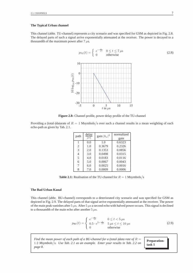
The Typical Urban channel

This channel (abbr. TU-channel) represents a city scenarioand was specified for GSM as depicted in Fig. 2.8.The delayed parts of such a signal arrive exponentially attenuated at the receiver. The power is decayed to athousandth of the maximum power after 7µs.

pTU(t) =

{

e−tµs 0 ≤ t ≤ 7 µs

0 otherwise(2.8)

-5 0 5 10 15-30

-20

-10

0

10

10log 1

0p

TU(t)

t in µs

Figure 2.8: Channel profile, power delay profile of the TU-channel

Providing a (total-)datarate ofR = 1 Msymbols/

s over such a channel results in a mean weighting of eachecho-path as given by Tab. 2.1.

normalizedpath delay[µs] gain|hν |

2

gain1 0.0 1.0 0.63232 1.0 0.3679 0.23263 2.0 0.1353 0.08564 3.0 0.0498 0.03155 4.0 0.0183 0.01166 5.0 0.0067 0.00437 6.0 0.0025 0.00168 7.0 0.0009 0.0006

Table 2.1: Realisation of the TU-channel forR = 1 Msymbols/

s

The Bad Urban Kanal

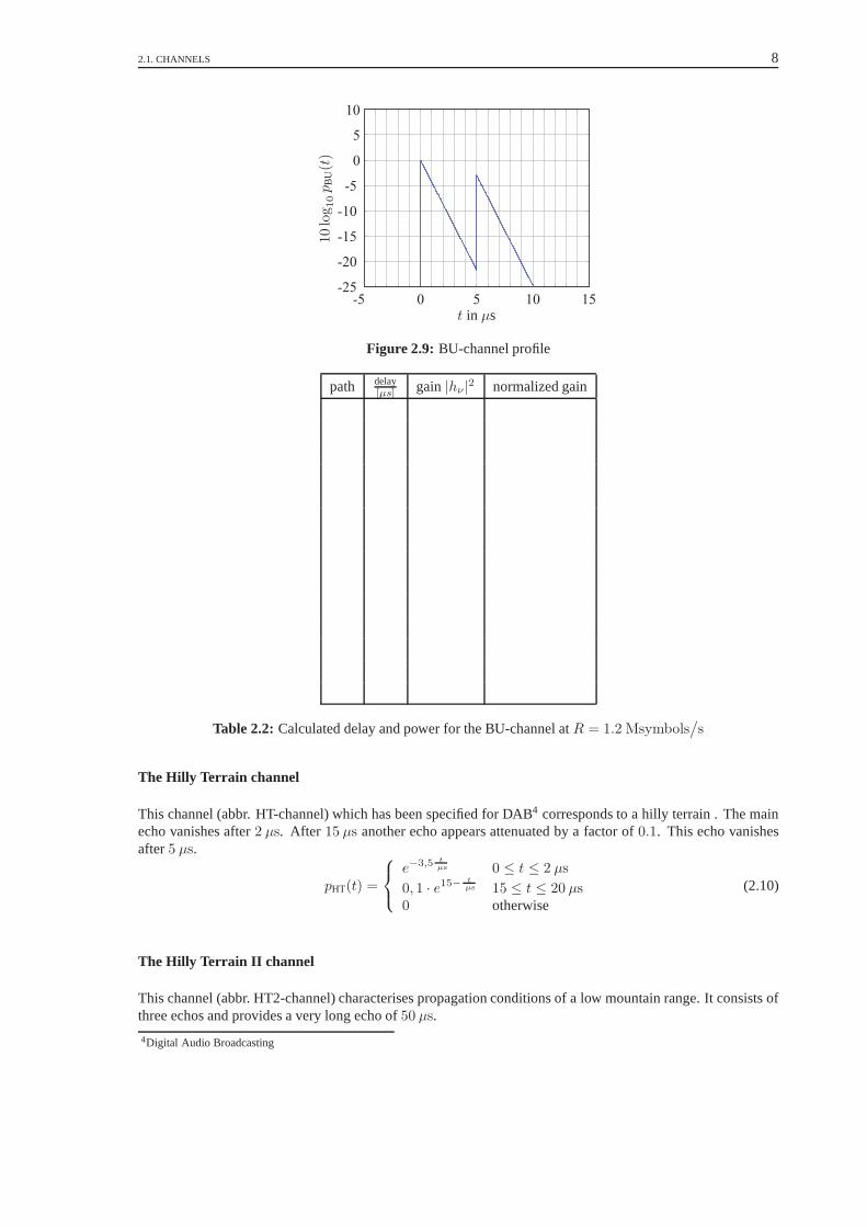
This channel (abbr. BU-channel) corresponds to a deteriorated city scenario and was specified for GSM asdepicted in Fig. 2.9. The delayed parts of that signal arriveexponentially attenuated at the receiver. The powerof the main peak vanishes after5 µs. After 5 µs a second echo with halved power occurs. This signal is declinedto a thousandth of the main echo after another5 µs.

pBU(t) =

e−tµs 0 ≤ t < 5 µs

0.5 · e5−tµs 5 µs ≤ t ≤ 10 µs

0 otherwise(2.9)

Find the mean power of each path of a BU-channel for a (total-)data rate ofR =1.2 Msymbols

/

s. Use Tab. 2.1 as an example. Enter your results in Tab. 2.2 onpage 8.

Preparation-task 1

2.1. CHANNELS 8

-5 0 5 10 15-25

-20

-15

-10

-5

0

5

10

10log 1

0p

BU(t)

t in µs

Figure 2.9: BU-channel profile

path delay[µs] gain|hν |

2 normalized gain

Table 2.2: Calculated delay and power for the BU-channel atR = 1.2 Msymbols/

s

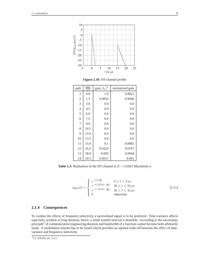
The Hilly Terrain channel

This channel (abbr. HT-channel) which has been specified forDAB4 corresponds to a hilly terrain . The mainecho vanishes after2 µs. After 15 µs another echo appears attenuated by a factor of0.1. This echo vanishesafter5 µs.

pHT(t) =

e−3,5 tµs 0 ≤ t ≤ 2 µs

0, 1 · e15−tµs 15 ≤ t ≤ 20 µs

0 otherwise(2.10)

The Hilly Terrain II channel

This channel (abbr. HT2-channel) characterises propagation conditions of a low mountain range. It consists ofthree echos and provides a very long echo of50 µs.

4Digital Audio Broadcasting

2.1. CHANNELS 9

-5 0 5 10 15 20 25-30

-25

-20

-15

-10

-5

0

5

10

10log 1

0p

HT(t)

t in µs

Figure 2.10: HT-channel profile

path delay[µs] gain|hν |

2 normalized gain

1 0.0 1.0 0.8821

2 1.5 0.0052 0.0046

3 3.0 0.0 0.0

4 4.5 0.0 0.0

5 6.0 0.0 0.0

6 7.5 0.0 0.0

7 9.0 0.0 0.0

8 10.5 0.0 0.0

9 12.0 0.0 0.0

10 13.5 0.0 0.0

11 15.0 0.1 0.0882

12 16.5 0.0223 0.0197

13 18.0 0.005 0.0044

14 19.5 0.0011 0.001

Table 2.3: Realisation of the HT-channel atR = 0.6667 Msymbols/

s

pHT2(t) =

e−2.3 tµs 0 ≤ t ≤ 3 µs

e−0.23(20− tµs ) 20 ≤ t ≤ 50 µs

e−1.72(40− tµs ) 40 ≤ t ≤ 44 µs

0 otherwise

(2.11)

2.1.4 Consequences

To combat the effects of frequency-selectivity a narrowband signal is to be preferred. Time-variance affectsespecially symbols of long duration, hence, a small symbol interval is desirable. According to the uncertaintyprinciple5 of communication engineering duration and bandwidth of a function cannot become both arbitrarilysmall. A modulation scheme has to be found which provides an optimal trade-off between the effect of time-variance and frequency-selectivity.

5Cf. [OL02], sec. 5.2.1

2.2. MULTI-CARRIER TRANSMISSION 10

0 10 20 30 40 50 60-30

-25

-20

-15

-10

-5

0

5

10

10log 1

0p

HT

2(t)

t in µs

Figure 2.11:HT2-channel profile

2.2 Multi-carrier transmission

2.2.1 Basic idea

We are considering a transmission of QPSK-data at a rate ofRS = 0.5 Msymbols/

s (corresponding to a band-width ofB = 0.5 MHz) over a Typical Urban channel. Duration of one symbol is given by∆TS = 1

RS= 2 µs.

Exhibiting a maximum delay ofτmax = 7 µs the TU-channel is associated with an impulse response of length⌈3.5⌉ = 4 (cf. Fig. 2.12 top). A corresponding Viterbi-equalizer would require the complexity of43 states.

By subdividing the bandwidth - as it is usual for multi-carrier systems - in for example10 sub-bands, each∆f = B/N = 50 kHz, a new symbol durationTS = 1

∆f = N/B = N∆TS = 20 µs comes up. The sameTU-channel would now distort only one additional symbol (cf. Fig. 2.12 below); the complexity of equalizationreduces to merely4 states per sub-channel.The reduction of the effects of a multi-path-channel (= frequency-selective channel) achieved by multi-carrier-systems can be illustrated in frequency domain. The individual sub-systems are now narrow-band resulting in anear-constant transfer-function of each sub-channel. Contrarily, a single-carrier transmission is distorted by thecomplete frequency-selective transfer-function. Hence,a multi-carrier system is able to decrease the influenceof frequency-selectivity.

single-carrier

multi-carrier

|h(t)|

B

B

t

t

t

f

f

TS = N · TSC

TSC

Figure 2.12: Realization of the same symbol-rate for single- and multi-carrier transmission

2.2. MULTI-CARRIER TRANSMISSION 11

The longer the duration of a symbol the stronger the effects of time-selectivity on our transmission become.The more sub-channels are used the more complex the implementation of a particular system becomes. Forthat reason sub-dividing our available bandwidth in sub-carriers is restricted to a certain extent.

2.2.2 Principle configuration

A multi-carrier system consists of transmitter and receiver as depicted in Fig. 2.13 and Fig. 2.14. The transmitter(Fig. 2.13) maps our bits after serial-parallel-conversion onto symbolsd[k, n],−∞ ≤ k ≤, 0 ≤ n ≤ N − 1∞and shapes corresponding impulses6 via gTx(t). After impulse shaping the modulation to each sub-carrier withfrequenciesf0 up tofN−1 takes place. Each sub-channel on its own forms a single-carrier-system. All sub-channels are then summed up. Thus a multi-carrier-signal arises which is now modulated with RF-frequencyand transmitted via our channel.

transmitter

.

.

.

Mod.

S/PSource

Map.

Map.

Map.

Map.ld(M) d[k, 0]

d[k, 1]

d[k, 2]

d[k,N -1]

ej2πf0t

ej2πf1t

ej2πf2t

ej2πfN−1t

gTx(t)

gTx(t)

gTx(t)

gTx(t)

x(t)

Figure 2.13: Principle setup of a MC-transmitter

The receiver (Fig. 2.14) is designed in a symmetrical mannerto the transmitter. Separating the sub-channelsis accomplished by demodulating with each sub-carrier frequency and filtering with the receiving filtergRx(t).Those filtersgRx(t) are best adapted togTx(t) resulting of a matched filter design7 as to maximize theS/N -ratio. After parallel-serial-conversion the received symbols d[k, n] are demapped and then assembled to thereceived bits.

Demap.

.

.

.

Mod.

P/S Sink

receiver

Demap.

Demap.

Demap.

y(t)

e−j2πf0t

e−j2πf1t

e−j2πf2t

e−j2πfN−1t

gRx(t)

gRx(t)

gRx(t)

gRx(t)

d[k, 0]

d[k, 1]

d[k, 2]

d[k,N -1]

ld(M)

Figure 2.14:Principle setup of a MC-receiver, without equalizer

Due to summing up all sub-channels the transmitting signalx(t) of a multi-carrier system is associated with acomplex envelope which is subject to strong variations resulting in enhanced prerequisites for the linearity of

6There are different approaches for impulse shaping. In Ch. 2.3 a closer look is taken.7Cf. [Kam96]

2.3. OFDM 12

the transmitting amplifier to produce an undistorted signal.

Regarding single-carrier transmission think of reasons for preferring π4 -

DPSK-modulation over0-DPSK-modulation. Why is Offset-QPSK especiallyadvantageous? Why are those considerations not important for multi-carrier-transmission?

Preparation-task 2

2.2.3 Interference

A MC-system like Fig. 2.13 and Fig. 2.14 suffers from non-adjusted impuls-shaping and sub-carrier-spacing;it is severely exposed to distortions. Those distortions are displayed in frequency domain as interchannel-interference ICI, arising from adjacent sub-channels, andin time domain as intersymbol-interference ISI,arising from influencing subsequent symbols (cf. Fig. 2.15). We will take a closer look at those disortionswithin the scope of OFDM (Ch. 2.3).

ICI ISI

t →

f→

Symbol−1 Symbol0 Symbol1

Figure 2.15: A multi-path-channel causes two forms of distortion, ISI and ICI

2.3 OFDM

OFDM8 terms a MC-system designed to combat ISI- and ICI-distortions. To achieve this a filter-function ischosen , which fulfills the first Nyquist criterion9 in time domain. The corresponding spectra are positioned inan orthogonal manner.

OFDM uses as finite time signal a rectangular pulse of lengthTS as transmitting and receiving filter10 (Fig. 2.16).

gTx(t) = gRx(t) = rect

(

t

TS

)

(2.12)

t0

1

∑

k

gTx(t)δ(t− kTS)

(k − 1)TS kTS (k + 1)TS

Figure 2.16: Impulse-shaping with non-overlapping time-signals

Due to the special impulse shaping the first Nyquist criterion is fulfilled leading to an always ISI-free OFDM-system. To enable ISI-resistance even for real multi-path-channels a so-called cyclic prefix is introduced.Its description is following below. Working with rectangular impulse an OFDM-system comprises infiniteextended sinc-shaped sub-channel-spectra.

8Orthogonal Frequency Division Multiplexing9cf. [Kam96], Sec. 2.1.2 and 5.2

10gTx(t) = gRx(t) is valid only if no cyclic-prefix is introduced.

2.3. OFDM 13

GTx(f) = GRx(f) = TS sinc(π f TS) (2.13)

The zeros of the sinc-function are positioned at frequenciesf = n/TS, n∈N. To design an ISI-free system thesub-channel-spectra are located at the zeros of their neighbors by chosing the distance between sub-channelsto ∆f = 1/TS. Hence, then-th sub-channel is associated with the modulation frequency fn = n∆f resultingin the typical setup of a OFDM spectrum in Fig. 2.17.

. . .

B = N/TS

f

f0 f1 f2 fN−1

Figure 2.17:Section of a OFDM-spektrum

2.3.1 OFDM-Transmitter

In the following the signal at transmitter output is developed.d[k, n] describes that symbol which is transmittedwithin then-th sub-channel of the vectord[k]. With Fig. 2.13 it is derived that

x(t) =

∞∑

k=−∞

N−1∑

n=0

d[k, n] · gTx(t− kTS)ej2πfnt. (2.14)

SettinggTx(t) to the impulse of Eq. (2.12) leads to

x(t) =∞∑

k=−∞

N−1∑

n=0

d[k, n] · rect

(

t− kTS

TS

)

ej2πfnt. (2.15)

W.l.o.g. we are regarding the OFDM-symbol with time-indexk = 0.

x(t) =

N−1∑

n=0

d[0, n]ej2πfnt fur 0 ≤ t < TS . (2.16)

In time-discrete processing a symbol of durationTS is sampledN times (t = ν TS

N ). With the sub-carrierspacingfn = n∆f = n 1

TSthe sampled transmitting signal corresponds to

x[ν] = x(νTS/N) with 0 ≤ ν ≤ N − 1.

Consideringfn = n/TS it follows that

x[ν] =

N−1∑

n=0

d[0, n]ej2πfnνTS/N

=

N−1∑

n=0

d[0, n]ej2πνn/N with 0 ≤ ν ≤ N − 1.

(2.17)

Finally we are taking all OFDM-symbols into account

x[k, ν] =

N−1∑

n=0

d[k, n]ej2πνn/N with 0 ≤ k ≤ N − 1 and −∞ < ν < ∞. (2.18)

2.3. OFDM 14

Eq. (2.18) is identical to the Inverse Fourier transform (IDFT). Hence, the transmitting front-end can becomposed of an IDFT-processor.

x[k] = N · IDFTN{d[k]} (2.19)

The functioning of Eq. (2.18) is illustrated by Fig. 2.18. Each timeN = 5 symbols are formed to a vectord[k]which is then via IFFT transformed into time domain where it is termed as vectorx[k].

d[0,0] d[0,1] d[0,2] d[0,3] d[0,4]d[-1,0] d[-1,1] d[-1,2] d[-1,3] d[-1,4] d[1,0] d[1,1] d[1,2] d[1,3] d[1,4]

x[0,0] x[0,1] x[0,2] x[0,3] x[0,4]x[-1,0] x[-1,1] x[-1,2] x[-1,3] x[-1,4] x[1,0] x[1,1] x[1,2] x[1,3] x[1,4]

k=0 k=1k=-1

d[0]d[−1] d[1]

x[0]x[−1] x[1]

Figure 2.18: Function of a OFDM-transmitter

d[k] andx[k] are describing vectors ofN symbols each.

d[k] = [d[k, 0], d[k, 1], . . . , d[k,N − 1]]T (2.20)

x[k] = [x[k, 0], x[k, 1], . . . , x[k,N − 1]]T (2.21)

2.3.2 OFDM-Receiver

We are taking a closer look at the receiving signaly(t). If it originates from the convolution of the channel-impulse-responseh(t) and the transmitting signalx(t), i.e.y(t) = x(t) ∗ h(t) then for the receiving signal atthe output of theµ-th receiving filter of theµ-th sub-channel it follows that

dµ(t) =(

y(t) e−j2πfµt)

∗ gRx(t). (2.22)

With fµ = µ∆f = µ/TS andgRx(t) = rect(

tTS

)

results

dµ(t) =(

y(t) e−j2πµ t

TS

)

∗ rect

(

t

TS

)

.

With the convolution integral11 we obtain

dµ(t) =1

TS

∞∫

−∞

y(τ) e−j2πµ τ

TS rect

(

t− τ

TS

)

dτ

=1

TS

t+TS∫

t

y(τ) e−j2πµ τ

TS dτ. (2.23)

Sampling att = 0 leads to

dµ(t)

∣

∣

∣

∣

t=0

=1

TS

TS∫

0

y(τ) e−j2πµ τ

TS dτ. (2.24)

11Due to the rectangular function of the receiving filter it is being integrated over one symbol interval.

2.3. OFDM 15

This equation for the receiving symbolsdµ(t)∣

∣

t=0is identical to the calculation of a Fourier series, i.e. the

spectrum of the receiving signaly(t) is being sampled at frequenciesfn = n/TA.

The OFDM-receiver reproduces a Fourier analysator which issampling the spectrum of the receiving signal.

Now we are approximating the integral of Eq.(2.24) by its lower sum

dµ(t)

∣

∣

∣

∣

t=0

≈1

TS

N−1∑

n=0

TA · y(nTA) e−j2πµ

nTATS . (2.25)

With sample periodeTA = TS/N the receiving signaly(t) is sampled

y[k, µ] = y(kTS + µTA). (2.26)

Hence, Eq.(2.24) yields

d[0, µ] =1

N

N−1∑

n=0

y[0, n] e−j2πµ nN mit 0 ≤ µ ≤ N − 1 (2.27)

Regarding all OFDM-symbols with indexk the instruction delivers

d[k, µ] =1

N

N−1∑

n=0

y[k, n] e−j2πµ nN , 0 ≤ µ ≤ N − 1 (2.28)

corresponding to the Discrete Fourier transform (DFT). Hence, similar to the transmitter the receiver can berealized by a DFT-processor.

d[k] =1

N· DFTN{y[k]} (2.29)

For an undistorted transmission the receiving data is identical to the transmitted data:

d[k] = DFTN{IDFTN{d[k]}} = d[k] (2.30)

The complete structure of multi-carrier transmitter and receiver in Fig. 2.13 and 2.14, respectively, is summa-rized in the easily implemented setup of Fig. 2.19.

Mapping IDFT DemappingDFTb[k]b[k]d[k] d[k]

n[k]

x[k] y[k]

Figure 2.19: Setup of OFDM transmitter and receiver for the AWGN-channel

2.3. OFDM 16

2.3.3 Cyclic Prefix

Transmitting over a frequency-selective channel causes the receiving signal to be superimposed by a channelecho. Hence, adjacent symbols are distorting each other. Fig. 2.20 illustrates this fact.ISI is caused at the head of each OFDM-symbol through the settling time of the preceding OFDM-symbol.Hence, parts of the preceding symbol are affecting the current symbol. ICI originates from channel influencesbetween sub-carriers of one OFDM-symbol.

Symbol 0 Symbol 1Symbol -1

receiving filter length

received symbols

transmitted symbols

transient phase (ISI)

transient phase (ICI)

|h(t)|t

t

0 TS 2TS

Figure 2.20: Multi-path propagation causes intersymbol-interference(ISI).

A possible way to circumvent echos is the periodic extensionof the transmitting signal, i.e. the extension ofthe symbol intervall with a cyclic prefix of lengthTG which should at least equal the maximum delay of thechannelτmax (cf. Fig. 2.21).The cyclic prefix is installed in form of a cyclic extension ofthe kernel symbol succeeding the IDFT, i.e. theend piece with lengthTG of each symbol in time domain is put in front of the symbol.

receiving filter length

received symbols

transmitted symbols

transient phase (ISI)

transient phase (ICI)

Symbol 0 Symbol 1Symbol -1

−T −TG 0 TS T t

|h(t)| |h(t− TS)|

Figure 2.21: Illustration of the cyclic prefix

2.3. OFDM 17

The impulse response of the transmitting filtergTx(t) is then given by

gTx(t) = rect

(

t

TS + TG

)

. (2.31)

But the cyclic prefix provides no new information resulting in a reduction of bandwidth-efficiency which isgiven by

u =duration of kernel symbol

duration of kernel + cyclic prefix=

TS

TS + TGsymbols/s/Hz (2.32)

bzw.

u =bits per OFDM-symbol

s/Hz=

TS

TS + TGlog2(M)bit/s/Hz (2.33)

Another disadvantage arises from the mismatching of transmitting and receiving filter. These are no longermatched causing an SNR-loss.

Determine the SNR-lossγ2 in dependance of the bandwidth-efficiencyu by use ofEq.(2.34)and the figure on the left hand side. Confirm thatγ2 ≤ 1 always holds.

Preparation-task 3

gRx(t)

gTx(t)

t

tTS + TG

TS

1

1

γ2 =

[

∞∫

−∞

gTx(τ)gRx(TS − τ)dτ

]2

∞∫

−∞

g2Tx(τ)dτ∞∫

−∞

g2Rx(τ)dτ(2.34)

The spectral power density of our white noise in the complex-valued baseband isN0, i.e. due to mismatchingan SNR-loss of

S/N = γ2 Es

N0= γ2 log2(M) ·Eb

N0(2.35)

is caused. From Eq.(2.34) follows at all timesγ2 ≤ 1. Think of the meaning. By adding a cyclic prefix we haveto spend more energy for transmitting one OFDM-symbol than without cyclic prefix. For a fair comparisonwith single-carrier transmission the total-energy has to be kept constant, hence, the energy per bit decreases ifthe noise power stays the same.

Explain the effect of the cyclic prefix.Hint: Think of the FFT-properties.

Preparation-task 4

Illustration of the cyclic-prefix

Fig.2.22 repeats once more the generation of the cyclic prefix. Following the IDFTNG symbols of the tailingend of our kernel symbol are attached to the head of the kernelsymbol prior to transmission.The cyclic prefix alters the linear convolution with the channel impulse response into a cyclic convolution.This is depicted in Fig.2.23. Pay particular notice to the convolution producty[0, 0] which results from theconvolution of kernel symbol headx[0, 0] and kernel symbol tailx[0, 4], x[0, 5].

2.3. OFDM 18

0

1

2

3

-2

-1

N-N

N

N

g

IDFT ...

.

………

kernel symbol cyclic prefix

n

x[k, n]

Figure 2.22: The cyclic prefix is built by attachingNG information symbols before the OFDM kernel symbol.Pay attention to the time directionn, i.e. the cyclic prefix is in deed transmitted prior to the kernelsymbol.

x[0,0] x[0,1] x[0,2] x[0,3] x[0,4] x[0,5]x[0,4] x[0,5]x[0,3]

kernel symbolcyclic prefix

OFDM symbol

h[1] h[0]h[2]

h[1] h[0]h[2]

h[1] h[0]h[2]

a)

b)

c)

d)

y[0,0] y[0,1] y[0,2] y[0,3] y[0,4] y[0,5]y[0,-2]y[0,-1]

y[0,-3]e)

y[0,5]=

transmitter

channel

receiver

*

=

ν →

Figure 2.23: a) After IDFT the cyclic prefix is attached to the kernel head.b,c,d) While transmitting over amulti-path channel ISI arises from convolution with the channelh[k]. e) The computing of theconvolution productsy[0,−1], y[0, 0] andy[0, 5] is hinted for three time instances.

2.3. OFDM 19

Cyclic prefix and linear algebra

This section considers a topic which is more or less unpopular among student, yet, is is very important, linearalgebra. We are studying an symbol rate OFDM system in complete matrix notation.First we are introducing the DFT-MatrixFN×N . Premultiplicating a vector withFN×N yields the fouriertransform of that vector, i.e.

FN×N · x = DFTN{x}. (2.36)

Correspondingly the IDFT resultsFH

N×N · x = N · IDFTN{x}. (2.37)

()H describes the Hermitian transposition. In MATLABFN×N is created by the commanddftmtx(N) .FH

N×N is generated bydftmtx(N)’ .

Inserting a cyclic prefix is achieved by premultiplying withmatrix G of dimension(NG + N × N). Thetransmission over a frequency-selective channel is described by premultiplying with the convolution matrixHof the channel. Hence, the receiving signaly[k] at the input of the OFDM receiver is

y[k] = HGFHx[k] + n[k]. (2.38)

For simplification we are considering vanishing noise, i.e.n[k] = 0. The receiver removes the cyclic prefixin the first place, what is accomplished by premultiplying matrix Ginv. Then the IDFT of the transmitter isreversed by premultipliying with the DFT-MatrixF .

FGinvy[k] = FGinvHGFHx[k] (2.39)

Of special form is the inner matrixGinvHG. It turns out that this is a so-calledcirculantmatrix, which we callH. Hence,

H = GinvHG. (2.40)

The easy equalization of OFDM relies on the following property of circulant matrixces. They are shaped intoa diagonal matrix by pre- and post-multiplication with DFT-and IDFT-matrices, i.e.

FHHF = diag{

H(

ej0)

, H(

ej2π/N)

, . . . , H(

ej2π(N−1)/N)}

. (2.41)

On the main diagonal the DFT-transform ofh[k] are positioned. By regarding Eq.(2.41) is becomes obviousthat the use of a cyclic prefix retains orthogonality betweenthe sub-carriers, i.e. each sub-carrier is independentof all other sub-carriers and each sub-carrier is just weighted by a factor of the channel transfer function.

OFDM receiver

IDFT add cyclic prefix channelremove cyclicprefix

DFT

OFDM transmitter

equalizationAWGN

d[k] d[k]

FH FGinvG H H−1

n[k]

x[k] y[k]

Figure 2.24:Symbol rate OFDM system

2.3. OFDM 20

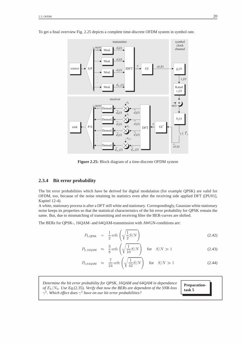
To get a final overview Fig. 2.25 depicts a complete time-discrete OFDM system in symbol rate.

DFT

TA

s(i,k)

.

.

.

sink

Demod.

Demod.

Demod.

Mod.Demod.ld( )M

~

~

~

~

n t( )

symbolclock

channel

+

( )h ta

transmitter

receiver

s i k( , )

.

.

.

S/Psource

Mod.

Mod.

Mod.

Mod.Mod.ld( )M

IDFT

N

s ta( )

Kanal( )c ta

( )g ta

GI-1

NGI

P/Sd i1( )

d i2( )

d iN-1( )

d i0( )

d i1( )

d i2( )

d iN-1( )

d i0( )

d i1( )

d i2( )

d iN-1( )

d i0( )e1

e2

eN-1

e0

Figure 2.25: Block diagram of a time-discrete OFDM system

2.3.4 Bit error probability

The bit error probabilities which have be derived for digital modulation (for example QPSK) are valid forOFDM, too, because of the noise retaining its statistics even after the receiving side applied DFT ([PU01],Kapitel 12-4).A white, stationary process is after a DFT still white and stationary. Correspondingly, Gaussian white stationarynoise keeps its properties so that the statistical characteristics of the bit error probability for QPSK remain thesame. But, due to mismatching of transmitting and receivingfilter the BER-curves are shifted.

The BERs for QPSK-, 16QAM- and 64QAM-transmission with AWGN-conditions are:

Pb,QPSK =1

2erfc

(

√

1

2S/N

)

(2.42)

Pb,16QAM ≈3

8erfc

(

√

1

10S/N

)

for S/N ≫ 1 (2.43)

Pb,64QAM ≈7

24erfc

(

√

1

42S/N

)

for S/N ≫ 1 (2.44)

Determine the bit error probability for QPSK, 16QAM and 64QAM in dependanceof Eb/N0. Use Eq.(2.35). Verify that now the BERs are dependent of the SNR-lossγ2. Which effect doesγ2 have on our bit error probabilities?

Preparation-task 5

21

Chapter 3

The OFDM system

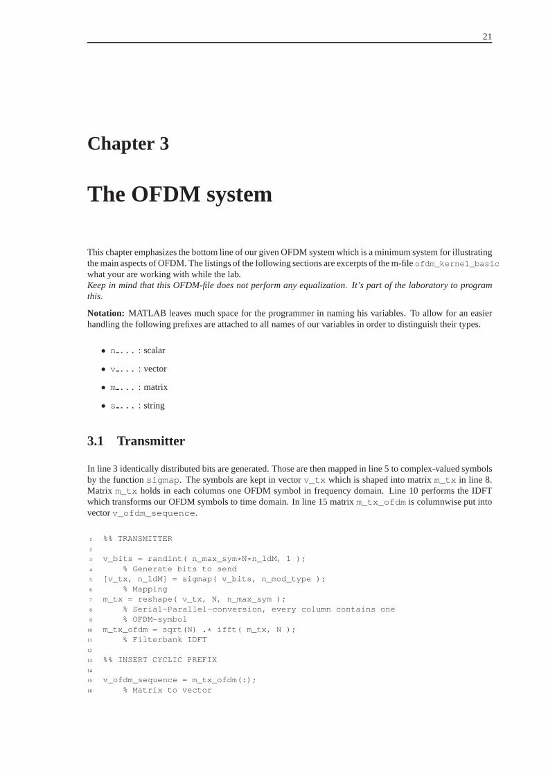
This chapter emphasizes the bottom line of our given OFDM system which is a minimum system for illustratingthe main aspects of OFDM. The listings of the following sections are excerpts of the m-fileofdm_kernel_basic

what your are working with while the lab.Keep in mind that this OFDM-file does not perform any equalization. It’s part of the laboratory to programthis.

Notation: MATLAB leaves much space for the programmer in naming his variables. To allow for an easierhandling the following prefixes are attached to all names of our variables in order to distinguish their types.

• n ... : scalar

• v ... : vector

• m... : matrix

• s ... : string

3.1 Transmitter

In line 3 identically distributed bits are generated. Thoseare then mapped in line 5 to complex-valued symbolsby the functionsigmap . The symbols are kept in vectorv_tx which is shaped into matrixm_tx in line 8.Matrix m_tx holds in each columns one OFDM symbol in frequency domain. Line 10 performs the IDFTwhich transforms our OFDM symbols to time domain. In line 15 matrix m_tx_ofdm is columnwise put intovectorv_ofdm_sequence .

1 %% TRANSMITTER2

3 v_bits = randint( n_max_sym * N* n_ldM, 1 );4 % Generate bits to send5 [v_tx, n_ldM] = sigmap( v_bits, n_mod_type );6 % Mapping7 m_tx = reshape( v_tx, N, n_max_sym );8 % Serial-Parallel-conversion, every column contains one9 % OFDM-symbol

10 m_tx_ofdm = sqrt(N) . * ifft( m_tx, N );11 % Filterbank IDFT12

13 %% INSERT CYCLIC PREFIX14

15 v_ofdm_sequence = m_tx_ofdm(:);16 % Matrix to vector

3.2. CHANNEL 22

3.2 Channel

The easiest channel consists of adding white Gaussian noise, the AWGN-channel. In line 19 the needed powern_sigma_sqr is being calculate. As one realisation of complex-valued noise vectorv_noise via theMATLAB-function randn is generated. In line 24 this noise is added after convoluting our transmittingsignal with the channel impulse reponse. Hence, at the receiving side we getv_ofdm_ch .

17 %% AWGN-channel18

19 n_sigma_sqr = 10ˆ(-n_EbN0_dB/10) * (N+Ng) / N / n_ldM ;20 % Noise-power21 v_noise = sqrt(n_sigma_sqr/2) * ( randn(size(v_ofdm_sequence)) ...22 + j * randn(size(v_ofdm_sequence)) );23 % Generate noise24 v_ofdm_ch = filter( v_channel, 1, v_ofdm_sequence ) + v_noi se;25 % Channel

3.3 Receiver

First, vector v_ofdm_ch is being shaped into matrixm_rx_ofdm_guard (line 28). Now matrixm_rx_ofdm keeps one OFDM-symbol in each column. In line 30 the transmitting side IDFT is reversedby a DFT. Right after putting matrixm_rx columnwise into vectorv_rx the complex-valued symbols are viasigdemap demapped to our originally sent bitsv_softbits_rx in line 34. Line 36 those soft-bits aretransformed into hard-decided bits. To find the symbol errorrate in line 38 the detected symbolsv_rx aregenerated out of the received bitsv_bits_rx .

26 %% RECEIVER27

28 m_rx_ofdm = reshape( v_ofdm_ch,N,length(v_ofdm_ch)/N);29 % Each column of ’m_rx_ofdm’ contains a OFDM-symbol30 m_rx = 1/sqrt(N) * fft(m_rx_ofdm);31 % Filterbank DFT32 v_rx = m_rx(:);33 % Matrix to vector34 v_softbits_rx = sigdemap( v_rx, n_mod_type );35 % Demapping36 v_bits_rx = v_softbits_rx>0;37 % Hard decision38 v_rx = sigmap( v_bits_rx, n_mod_type );39 % Remodulate to find SER

3.4 Evaluation

Evaluation is done essentially via the˜= -operator. Two sequences are checked for inequality resulting in abinary vector. By way of the mean value of this vector we find bit error rate as well as symbol error rate.

40 v_ber(ebn0_cnt) = mean( v_bits_rx(:)˜=v_bits(:) );41 v_ser(ebn0_cnt) = mean( v_rx˜=v_tx );

23

Chapter 4

Task execution

You are going to start this task with a basic OFDM system whichis provided to you as the functionofdm_kernel_basic.m . The cyclic prefix has not been taken care of, yet. The channelconsists of addingwhite Gaussian noise (AWGN) only.Your task is to extend the OFDM system’s functionality. Furthermore, you are modifying transmitter andreceiver with regard to the cyclic prefix. You are going to encounter signs likePlot on the margin indicatingthat you should print your current plot. Answer in short the corresponding questions to each plot.

The interface of our OFDM system is

[n_ber,n_ser] = ofdm_kernel_basic(n_EbN0_dB,n_u0,N,n_ max_sym,n_mod_type,v_channel)

The parameters are

n ber,n ser BER, SER

n EbN0 dB Bitenergy per noise power in dBn u0 bandwidth-efficiencyN Number of sub-carriersn max sym Number of OFDM symbolsn mod type Modulation (2=QPSK,4 = 16QAM, 5 = 16PSK,6 = 64QAM)v channel channel impulse response

The following variables are important to all subsequent tasks:

N Number of sub-carrierslog2 M bits per symbolRb data-rateu bandwidth-efficiency

Think of how these variables can by used to compute the following values:

• durationT of total symbol inµs,

• durationTS of kernel symbol inµs,

• durationTG of cyclic prefix inµs,

• sampling periodTA in µs,

• durationNS = ⌈TS/TA⌉ in taps of kernel symbol,

• cyclic prefixNG = ⌈TG/TA⌉ in taps

Preparation-task 6

4.1. TASK 1: TRANSMISSION OVER THE AWGN-CHANNEL 24

4.1 Task 1: Transmission over the AWGN-channel

You are going to compare simulated and theoretical bit errorcurves for transmission over AWGN.

4.1.1 Without cyclic prefix

1. Start with implementing a framework aroundofdm_kernel_basic.m . Open a new filetask1.m .For the first line of your new file enterfigure; clear all; dbstop if error .

2. Assign withintask1.m the following variables

N=256; You are using256 sub-carriers.u0=1; Bandwidth-efficiency is ”1”.

Keep in mind, that you yet have to add the functionality of thecyclic prefix.n max sym=100; The number of OFDM symbols decides for the precision of your results.n mod type=2; Modulation (2 =QPSK,4 = 16QAM, 6 = 64QAM)v channel=[1]; channel impulse response; here, the channel is ideal.

3. Assign a vectorv_EbN0_dB=[0:10]; .

4. Within afor -loop grab the components ofv_EbN0_dB assigning them ton_EbN0_dB. Remember ina vectorv_ber all simulated bit error rates.

v_ber=[];for n_EbN0_dB=v_EbN0_dB

[n_ber,n_ser] = ofdm_kernel_basic(<substitute list of pa rameters>);v_ber = [v_ber n_ber];

endsemilogy(v_EbN0_dB,v_ber);

Now you have provided all parameters for callingofdm_kernel_basic within the loop. This functionsimulates now for eachEb/N0 in dB the bit error raten_ber and the symbol error raten_ser .

5. Plot additionally the simulated BER-dots viasemilogy(n_EbN0_dB,n_ber,’o’); by insertingthis command right after callingofdm_kernel_basic . To not erase the previously plotted points,inserthold on; drawnow; .

By now you should have produced a working program. Give it a try and run your simulation but do not printthis plot yet.

6. To verify your results plotafter the loop the theoretical bit error probability of Eq.(2.42). Mind the SNRof Eq.(2.35). Use your result of preparation-task 5.

Hint: Pay attention to the bit error probability which requires the linear Eb/N0-ratio. The variablen_mod_type is identical to the number of bits per symbollog2 M . Proceed like this:

v_EbN0 = <Umrechnungconversion of v_EbN0_dB to linear scal e>v_ber = <Computation of BER in eq. (2.42) as function of v_EbN0>semilogy(v_EbN0_dB, v_ber,’--’);

The theoretical and the simulated points should coincide provided you’ve programmed properly.

7. Change the mapping by means ofn_mod_type .Use 16QAM (n mod type=4; ) and 64QAM (n mod type=6; ). Therefore, generate a vectorv mod type=[2 4 6]; in your function-header. Now, put a secondfor -loop around your first loopand your plot-command and assign the elements ofv_mod_type to n_mod_type within this newloop.

If you are running your programm right now, simulated and theoretical curves are (not yet) falling together. Forthat you have to process the remaining item.

4.1. TASK 1: TRANSMISSION OVER THE AWGN-CHANNEL 25

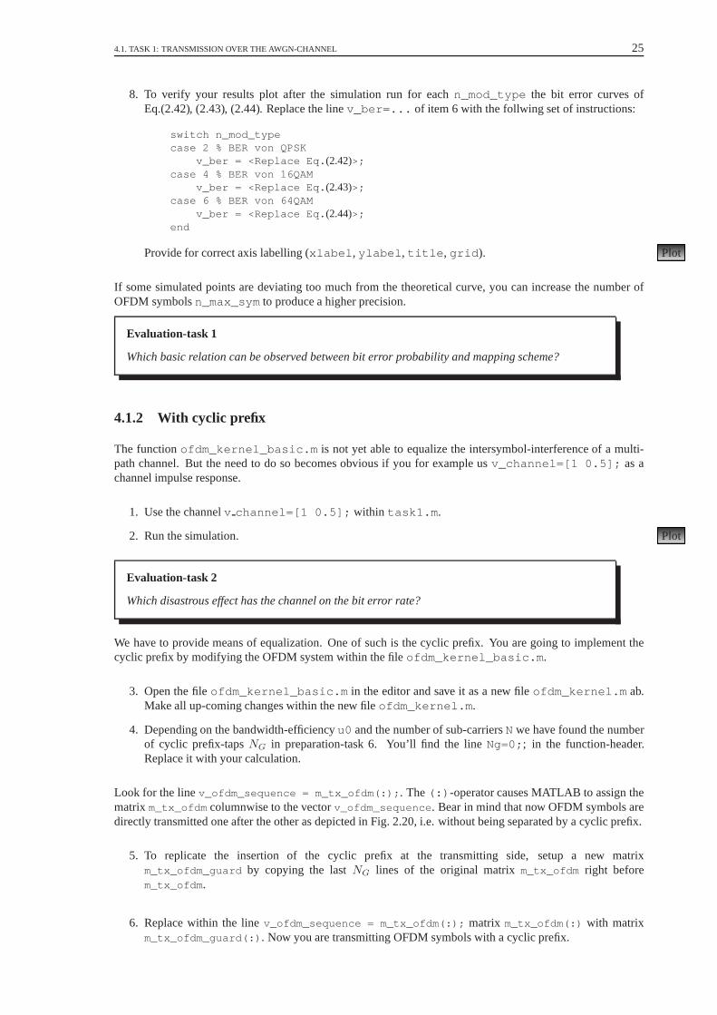
8. To verify your results plot after the simulation run for each n_mod_type the bit error curves ofEq.(2.42), (2.43), (2.44). Replace the linev_ber=... of item 6 with the follwing set of instructions:

switch n_mod_typecase 2 % BER von QPSK

v_ber = <Replace Eq. (2.42)>;case 4 % BER von 16QAM

v_ber = <Replace Eq. (2.43)>;case 6 % BER von 64QAM

v_ber = <Replace Eq. (2.44)>;end

Provide for correct axis labelling (xlabel , ylabel , title , grid ). Plot

If some simulated points are deviating too much from the theoretical curve, you can increase the number ofOFDM symbolsn_max_sym to produce a higher precision.

Evaluation-task 1

Which basic relation can be observed between bit error probability and mapping scheme?

4.1.2 With cyclic prefix

The functionofdm_kernel_basic.m is not yet able to equalize the intersymbol-interference ofa multi-path channel. But the need to do so becomes obvious if you for example usv_channel=[1 0.5]; as achannel impulse response.

1. Use the channelv channel=[1 0.5]; within task1.m .

2. Run the simulation. Plot

Evaluation-task 2

Which disastrous effect has the channel on the bit error rate?

We have to provide means of equalization. One of such is the cyclic prefix. You are going to implement thecyclic prefix by modifying the OFDM system within the fileofdm_kernel_basic.m .

3. Open the fileofdm_kernel_basic.m in the editor and save it as a new fileofdm_kernel.m ab.Make all up-coming changes within the new fileofdm_kernel.m .

4. Depending on the bandwidth-efficiencyu0 and the number of sub-carriersNwe have found the numberof cyclic prefix-tapsNG in preparation-task 6. You’ll find the lineNg=0; ; in the function-header.Replace it with your calculation.

Look for the linev_ofdm_sequence = m_tx_ofdm(:); . The(:) -operator causes MATLAB to assign thematrix m_tx_ofdm columnwise to the vectorv_ofdm_sequence . Bear in mind that now OFDM symbols aredirectly transmitted one after the other as depicted in Fig.2.20, i.e. without being separated by a cyclic prefix.

5. To replicate the insertion of the cyclic prefix at the transmitting side, setup a new matrixm_tx_ofdm_guard by copying the lastNG lines of the original matrixm_tx_ofdm right beforem_tx_ofdm .

6. Replace within the linev_ofdm_sequence = m_tx_ofdm(:); matrix m_tx_ofdm(:) with matrixm_tx_ofdm_guard(:) . Now you are transmitting OFDM symbols with a cyclic prefix.

4.1. TASK 1: TRANSMISSION OVER THE AWGN-CHANNEL 26

Visualize that now a situation as depicted in Fig. 2.21 is given. Each OFDM symbol has been extended byattaching a cyclic prefix in front of it. At the receiving sidethis cyclic prefix has to be removed.

7. Look for the linem_rx_ofdm=reshape( v_ofdm_ch, N, length(v_ofdm_ch)/N ); . The com-mandreshape shapes a vector into a matrix. Adjust this command in such waythat each column keepsone OFDM symbol.Hint: A OFDM symbol consists now of the kernel symbol plus cyclic prefix.

8. Remove now all cyclic prefixes in front of the OFDM symbols by assigning the kernel symbols only tomatrixm_rx_ofdm , i.e. all rowsafter the cyclic prefix.

It follows the programming of the actual equalization.

9. Look for the linem_rx=1/sqrt(N) * fft(m_rx_ofdm); . Setup a vectorv_eq which you are assigningto the FFT of the channel impulse responsev_channel . Think of the correct length for the FFT.

10. Multiply this equalization-vectorv_eq into a matrix m_eq. For that use the commandm_eq=repmat(v_eq(:),1,size(m_rx,2)); so that the dimensions ofm_eq fit to the OFDM matrixm_rx . Carry out the actual equalization by dividingm_rx by m_eq.

By now you’ve got a complete OFDM system.

11. Stick to the multi-path channelv_channel=[1 0.5]; . To see your work’s result, use a bandwidth-efficiency ofu0=.95; in your file task1.m . Change the call ofofdm_kernel_basic to the previ-ously adjustedofdm_kernel . Provide correct axis labelling (xlabel , ylabel , title , grid ). Plot

Evaluation-task 3

Compare the current plot and the previous plot. Make a qualitative statement about the generaltrend of the bit error rates with and without equalization toeach other and to the AWGN curves.

4.2. TASK 2: BANDWIDTH-EFFICIENCY 27

4.2 Task 2: Bandwidth-efficiency

The cyclic prefix means redundancy. Energy has to be providedwhich is of no further use at the receiver.Compared to a single carrier system we observe an SNR-loss which becomes the bigger the longer the cyclicprefix is chosen.The conduct of OFDM under varying bandwidth-efficiency and different channel conditions shall be examined.

4.2.1 AWGN-channel

Start with the AWGN-channel.

1. Save your filetask1.m as a new filetask2.m ab and work with this new file. Useofdm kernelinstead ofofdm kernel basic.

2. Setv_channel=[1]; . Such you’re using an AWGN-channel.

3. Assign a vectorv_u=[0.5:0.1:1]; . This vector contains the bandwidth-efficienciesu that are to beexamined.

4. Enclose the loopn_mod_type=v_mod_type within a new loop, i.e.

<simulation parameter>for u0 = v_u

<function-body of task1.m>end

5. Begin with QPSK und setv_mod_type = [2]; .

6. Start the simulation. Should the simulated points deviate too much from the theoretical curves the numberof OFDM symbolsn_max_sym can be increased.

7. After running the simulation adjust viaaxis([0 10 1e-5 1]) the range of the current figure. Plot

8. Repeat item 5.-7. for16QAM (n_mod_type=4; ) and 64QAM (n_mod_type=6; ). Plot2×

Evaluation-task 4

What is the influence of the bandwidth-efficiency in regard ofthe bit error probability of all threemapping-schemes?Compare the bit error rates of all mapping-schemes with eachother. Which scheme performs best?Why?

4.2. TASK 2: BANDWIDTH-EFFICIENCY 28

4.2.2 Multi-path channel

You are going to examine your OFDM system with two channel impulse responses which are specified in theGSM standard, HT- and TU-channel.

Find the maximum bandwidth-efficiency for the TU- and HT-channel with a givennumber of sub-channels ofN = 256 and a data-rate ofRb = 8.192Mbit/s providedthat the cyclic prefix covers the whole channel impulse response. Mapping=QPSK.

uTU,max =uHT,max =

Preparation-task 7

Compute the values for cyclic prefix-duration and symbol-duration and enter theminto the table below. Assume again a number of sub-carriersN = 256 and adata-rate ofRb = 8.192 Mbit/s. QPSK

Preparation-task 8

u 0.5 0.6 0.7 0.8 0.9 1.0

TS in µs

TG in µs

TA in µs

TG/TA in taps (ceil)

length of TU-cir in taps

length of HT-cir in taps

cyclic prefix sufficient (TU)?

cyclic prefix sufficient (HT)?

1. Change the range of the simulatedEb/N0’s to v_ebn0_db=0:2:20; .

2. Assign in the function-headeroftask2.m the variabless_channel=’HT’; andn_Rbit=8.192e6; .

3. Calculate right after the linefor n_mod_type=v_mod_type the needed sampling-periodn_Ta .Use your result of preparation-task 6.

4. By using the routineofdm_channel you obtain GSM-channel impulse reponses. Use the commandv_channel=ofdm_channel(s_channel,n_Ta); after calculatingn_Ta .

5. Comment via%the plot-command of the theoretical bit error curves. They are no longer valid for ISI-introducing channels.

6. Run the simulation. Plot

7. Now simulate the transmission over the TU-Kanal via settings_channel=’TU’; and run the simula-tion again. Plot

4.2. TASK 2: BANDWIDTH-EFFICIENCY 29

Evaluation-task 5

• Do the bit error rates conduct like expected?

• Why do the bit error rates saturate at higherEb/N0?

• To what extent are the channel impulse responses influencinga symbol at different bandwidth-efficiencies? Regard that parts of power which fall inside and outside of the cyclic prefix andthe distorting part compared to the total symbol-duration.What would be the effect for asingle-carrier transmission with the same data-rate andTA ≈ const.? Use Fig. 2.12 forhelp.

• Why should the cyclic prefix in mobile transmissions at leastcover the channel impulseresponse?

4.3. TASK 3: NUMBER OF SUB-CARRIERS 30

4.3 Task 3: Number of sub-carriers

You’re going to examine the influence of the sub-carriersN for a constant bandwidth-efficiencyu = 0.85 onthe bit error rates. Simulations are for the BU- and the HT-channel.

Calculate the values for cyclic prefix and symbol-duration (now for a 16QAM-transmission) and enter your results into the table below (Rb = 8.192 Mbit/s).Which number of sub-carrier will produce the smallest bit error rates?

Preparation-task 9

N 16 32 64 128 256 512 1024

TS in µs

TG in µs

TA in µs

TG/TA in taps (ceil)

BU-cir in taps

HT-cir in taps

cyclic prefix sufficient (BU)?

cyclic prefix sufficient (HT)?

Summarize how many sub-carriers you have to provide at leastto have a sufficiently large cyclic prefix.

NBU ≥

NHT ≥

1. Start with savingtask2.m astask3.m . Work with this new file.

2. If you have not done so yet, remove all lines addressing thetheoretical bit error probabilities for theAWGN-channel. They are not of interest here.

3. Assign in the function-header a vectorv_N=[16 32 64 128 256 512]; . Those numbers of sub-carriers are to be simulated.

4. Assign the bandwidth-efficiencyu0=0.85; .

5. Change the loop-headerfor u0=v_u into for N=v_N .

6. Start with the BU-chanel and sets_channel=’BU’; .

7. Transmit200 OFDM symbols, i.e.n_max_sym=200;

8. Use 16QAM, i.e.v_mod_type=[4] .;

9. Run the simulation. Plot

10. Simulate now the HT-channel and sets_channel=’HT’; . Plot

Evaluation-task 6

• Explain the trend of the bit error curves. Consider the partsof the channel impulse powerinside and outside of the cyclic prefix.

• Generally what can you observe in regard of the ratio betweenbit error rate and number ofsub-carriers? How many sub-carriers should be chosen?

4.4. TASK 4: DIFFERENT CHANNEL MODELS AND DIFFERENT MAPPINGS 31

4.4 Task 4: Different channel models and different mappings

Under the premise of a cyclic prefix that covers the channel impulse responsecompletely calculate the maximum bandwidth-efficiency forthe given mappings,number of sub-channels and channel-types. Furthermore, calculate the length ofthe cyclic prefix in taps andµs, the kernel symbol durationTS and the total symboldurationT . The data-rate isRb = 0.512Mbit/s.

Preparation-task 10

TU-channel BU-channel HT-channel HT2-channel

N 32 32 32 32

umax

T in µs

QPSK TS in µs

TG in µs

TA in µs

TG/TA in taps

umax

16PSK T in µs

& TS in µs

16QAM TG in µs

TA in µs

TG/TA in taps

4.4.1 Different channel models

In this task you’ll check the influence of the channel’s frequency-selectivity on your OFDM system. You willplot the bit error rates vs.Eb/N0 in dB as well as the channel transfer function.

1. Savetask3.m as new filetask4.m and work with this new file.

2. Insert as first lineclose all; figure(1); figure(2); ein. After closing all opened windowsyou’re opening two new windows.

3. Replace vectorv_N=[...]; with the number of sub-carriersN=32; .

4. Use QPSK, i.e.v_mod_type=[2]; .

5. Change the data-rate ton_Rbit=.512e6; .

6. Replace vectorv_ebn0_db=[0:2:20]; .

7. Change loop-headerfor N=v_N into for n_id=0:3 .

8. Enter right after the loop-header the following instructions

switch n_idcase 0

s_channel = ’TU’;s_color = ’vb-’;u0 = <Your value>;

case 1s_channel = ’BU’;s_color = ’sr-’;u0 = <Your value>;

4.4. TASK 4: DIFFERENT CHANNEL MODELS AND DIFFERENT MAPPINGS 32

case 2s_channel = ’HT’;s_color = ’ˆg-’;u0 = <Your value>;

case 3s_channel = ’HT2’;s_color = ’ok-’;u0 = <Your value>;

end

9. By use of the strings_color you can mark your simulation results individually. Replacethe plot-command within the loop for n_EbN0_dB=v_ebn0_db withsemilogy(n_EbN0_dB,n_ber,s_color); and the plot-commandafter the loop withsemilogy(v_ebn0_db,v_ber,s_color)

10. Insert after the linev_channel=ofdm_channel(s_channel,n_Ta); the following instructions:

figure(1)plot(abs(fftshift(fft(v_channel,N))),s_color)hold onfigure(2)

By means of that you’re displaying the transfer function of the current channel in the first window.

11. Run the simulation. Plot the channel transfer functionsand the bit error curves. Plot2×

Evaluation-task 7

• Explain the different trends of the bit error curves.

• Explain the relation between bit error curves and channel transfer functions.

4.4.2 Different mappings

The Hilly Terrain channel (HT-channel) is to be simulated for different mapping-schemes.

1. Savetask3.m astask4a.m .

2. Changes_channel=’HT’ .

3. Changev_N=[32]; .

4. Changev_mod_type=[2 4 5]; , so you’re simulating QPSK,16QAM and16PSK.

5. Run the simulation. Plot

Evaluation-task 8

• Why are higher-level mapping-schemes more error-prone than QPSK if transmission over antime-variant channel is considered?

• Nevertheless when is a higher-level mapping sensible?

BIBLIOGRAPHY 33

Bibliography

[Kam96] K. D. Kammeyer.Nachrichtenubertragung. Teubner, Stuttgart, 2. edition, 1996.

[OL02] J.-R. Ohm and H. D. Luke.Signalubertragung. Springer-Verlag, Berlin, 8. edition, 2002.

[PU01] A. Papoulis and S. Unnikrishna.Probability, Random Variables, and Stochastic Processes. McGraw-Hill, 4.edition, 2001.