Communications in Applied Mathematics and Computational ... · Communications in Applied...
152
Communications in Applied Mathematics and Computational Science vol. 5 no. 1 2010 mathematical sciences publishers
Transcript of Communications in Applied Mathematics and Computational ... · Communications in Applied...

Communications inAppliedMathematics andComputationalScience
vol. 5 no. 1 2010
mathematical sciences publishers

Communications in Applied Mathematics and Computational Sciencepjm.math.berkeley.edu/camcos
EDITORS
MANAGING EDITOR
John B. BellLawrence Berkeley National Laboratory, USA
BOARD OF EDITORS
Marsha Berger New York [email protected]
Alexandre Chorin University of California, Berkeley, [email protected]
Phil Colella Lawrence Berkeley Nat. Lab., [email protected]
Peter Constantin University of Chicago, [email protected]
Maksymilian Dryja Warsaw University, [email protected]
M. Gregory Forest University of North Carolina, [email protected]
Leslie Greengard New York University, [email protected]
Rupert Klein Freie Universitat Berlin, [email protected]
Nigel Goldenfeld University of Illinois, [email protected]
Ahmed Ghoniem Massachusetts Inst. of Technology, [email protected]
Raz Kupferman The Hebrew University, [email protected]
Randall J. LeVeque University of Washington, [email protected]
Mitchell Luskin University of Minnesota, [email protected]
Yvon Maday Universite Pierre et Marie Curie, [email protected]
James Sethian University of California, Berkeley, [email protected]
Juan Luis Vazquez Universidad Autonoma de Madrid, [email protected]
Alfio Quarteroni Ecole Polytech. Fed. Lausanne, [email protected]
Eitan Tadmor University of Maryland, [email protected]
Denis Talay INRIA, [email protected]
PRODUCTION
Paulo Ney de Souza, Production Manager Sheila Newbery, Production Editor Silvio Levy, Senior Production Editor
See inside back cover or pjm.math.berkeley.edu/camcos for submission instructions.
The subscription price for 2010 is US $70/year for the electronic version, and $100/year for print and electronic. Subscriptions, requestsfor back issues from the last three years and changes of subscribers address should be sent to Mathematical Sciences Publishers,Department of Mathematics, University of California, Berkeley, CA 94720-3840, USA.
Communications in Applied Mathematics and Computational Science, at Mathematical Sciences Publishers, Department of Mathemat-ics, University of California, Berkeley, CA 94720-3840 is published continuously online. Periodical rate postage paid at Berkeley, CA94704, and additional mailing offices.
CAMCoS peer-review and production is managed by EditFLOW™ from Mathematical Sciences Publishers.
PUBLISHED BYmathematical sciences publishers
http://www.mathscipub.orgA NON-PROFIT CORPORATION
Typeset in LATEXCopyright ©2010 by Mathematical Sciences Publishers

COMM. APP. MATH. AND COMP. SCI.Vol. 5, No. 1, 2010
FETI AND BDD PRECONDITIONERS FORSTOKES–MORTAR–DARCY SYSTEMS
JUAN GALVIS AND MARCUS SARKIS
We consider the coupling across an interface of a fluid flow and a porous mediaflow. The differential equations involve Stokes equations in the fluid region,Darcy equations in the porous region, plus a coupling through an interface withBeaver–Joseph–Saffman transmission conditions. The discretization consists ofP2/P1 triangular Taylor–Hood finite elements in the fluid region, the lowestorder triangular Raviart–Thomas finite elements in the porous region, and themortar piecewise constant Lagrange multipliers on the interface. We allow fornonmatching meshes across the interface. Due to the small values of the per-meability parameter κ of the porous medium, the resulting discrete symmetricsaddle point system is very ill conditioned. We design and analyze precondi-tioners based on the finite element by tearing and interconnecting (FETI) andbalancing domain decomposition (BDD) methods and derive a condition num-ber estimate of order C1(1+ (1/κ)) for the preconditioned operator. In casethe fluid discretization is finer than the porous side discretization, we derive abetter estimate of order C2((κ + 1)/(κ + (h p)2)) for the FETI preconditioner.Here h p is the mesh size of the porous side triangulation. The constants C1 andC2 are independent of the permeability κ , the fluid viscosity ν, and the meshratio across the interface. Numerical experiments confirm the sharpness of thetheoretical estimates.
1. Introduction
We consider the coupling across an interface of a fluid flow and a porous mediaflow. The model consists of Stokes equations in the fluid region, Darcy equationsfor the filtration velocity in the porous medium, and an adequate transmission con-dition for coupling of these equations through an interface. Such problems appearin several applications such as well-reservoir coupling in petroleum engineering,transport of substances across groundwater and surface water, and (bio)fluid-organinteractions. There are works that address numerical analysis issues of this model.For inf− sup conditions and approximation results associated to the continuous and
MSC2000: 35Q30, 65N22, 65N30, 65N55, 76D07.Keywords: Stokes–Darcy coupling, mortar, balancing domain decomposition, FETI, saddle point
problems, nonmatching grids, discontinuous coefficients, mortar elements.
1

2 JUAN GALVIS AND MARCUS SARKIS
discrete formulations for Stokes–Laplacian systems we refer [15; 12], for Stokes–Darcy systems we refer [31; 39; 2; 22], for Stokes–Mortar–Darcy systems, see [41;26], and for DG discretizations [11; 41]. For studies on preconditioning analysisfor Stokes-Laplacian systems, see [13; 14; 16; 17], and for Stokes-Darcy systems[3]. In this paper, we are interested in balancing domain decomposition (BDD)and finite element by tearing and interconnecting (FETI) preconditioned conjugategradient methods for Stokes–Mortar–Darcy systems. For general references onBDD and FETI type methods, see [18; 19; 23; 24; 30; 33; 34; 35; 36; 40; 42; 43;44].
In this paper we both extend some preliminary results contained in [25] and intro-duce and analyze new methods. We note that the BDD-I preconditioner introducedin [25] is not effective for small permeabilities (in real applications permeabilitiesare very small) while the preconditioner BDD-II in [25] requires constructing inter-face base functions which are orthogonal in the Stokes inner product (this construc-tion is very expensive and impractical because it requires, as a precomputationalstep, solving many Stokes problems). Here in this paper we circumvent theseissues by introducing a dual formulation and considering FETI-based methods. Wepropose and analyze FETI methods and present numerical experiments in order toverify the theory. We note that the analysis of the FETI algorithms for Stokes–Mortar–Darcy problems is very challenging due to the following issues:
(i) the mortar map from the Stokes to the Darcy side has a large kernel since theStokes velocity space is in general richer than the Darcy velocity space on theinterface;
(ii) the trace space of the Stokes velocity (H 1/2) is more regular than the tracespace of the Darcy flux (H−1/2), and due to a priori error estimates [31; 41;26], the Stokes side must be chosen as the master side;
(iii) the energy associated to the Darcy region is much larger than the energy as-sociated to the Stokes region due to the small value of the permeability.
Such issues imply that the master side must be chosen on the Stokes side and wherethe energy is smaller and velocity space is richer. The mathematical analysis underthis choice is very hard to analyze even for simpler problems such as for transmis-sion problems with discontinuous coefficients using Mortar or DG discretizations[19; 20; 21]. For problems where both the smallest coefficient and the finest meshare placed on the master side, as far as we know, there are no optimal precondi-tioners developed in the literature for transmission problems, and typically there isa condition to rule out such a choice.
The rest of the paper is organized as follows: in Section 2 we present the Stokes–Darcy coupling model. In Section 3 we describe the weak formulation of thismodel. In Section 4 we introduce a finite element discretization. In Section 5 we
FETI AND BDD PRECONDITIONERS FOR STOKES–MORTAR–DARCY SYSTEMS 3
study the primal and dual formulation of the discrete problem. Section 6 presentsa complete analysis of the BDD-I preconditioner introduced in [25]. In Section 7,we design and analyze the FETI preconditioner; see Lemma 3 and Theorem 4. Inparticular we obtain the condition number estimate of order C1(1+(1)/(κ)) for thispreconditioner and also prove Theorem 7, which gives a better estimate of orderC2((κ+1)/(κ+ (h p)2)) for the FETI preconditioner in case the fluid discretizationis finer than the porous side discretization; the case where the Stokes mesh is nota refinement of the Darcy mesh is also discussed (see Remark 8). In Section 7we also consider more general fluid bilinear forms by allowing the presence of atangential interface fluid velocity energy (Remark 10), and also translate the FETIresults to analyze certain BDD methods (Remark 9). In Section 8 we present thenumerical results, and in Section 9 we discuss the multisubdomain case.
Here h p is the mesh size of the porous side triangulation. The constants C1 andC2 are independent of the permeability κ , the fluid viscosity ν, and the mesh ratioacross the interface. In Section 8 we present numerical results that confirm thetheoretical estimates concerning the BDD and the FETI preconditioners.
2. Problem setting
Let � f , �p⊂ Rn be polyhedral subdomains, define � := int(�
f∪�
p) and 0 :=
∂� f∩ ∂�p, with outward unit normal vectors ηi on ∂�i , i = f, p. The tangent
vectors on 0 are denoted by τ1 (n = 2), or τl , l = 1, 2 (n = 3). The exteriorboundaries are 0i
:= ∂�i\0, i = f, p. Fluid velocities are denoted by ui
:�i→Rn ,
i = f, p, and pressures by pi:�i→ R, i = f, p.
We consider Stokes equations in the fluid region � f and Darcy equations for thefiltration velocity in the porous medium �p. More precisely, we have the followingsystems of equations in each subdomain:
Stokes equations Darcy equations−∇ · T (u f , p f ) = f f in � f ,
∇ · u f= g f in � f ,
u f= h f on 0 f ,
up=−
κν∇ p p in �p,
∇ · up= g p in �p,
up· ηp= h p on 0 p.
(1)
Here T (v, p) :=−pI+2νDv, where ν is the fluid viscosity, Dv := 12(∇v+∇vT ) is
the linearized strain tensor and κ denotes the rock permeability. For simplicity onthe analysis, we assume that κ is a real positive constant. We impose the followingconditions:
(1) Interface matching conditions across 0; see [15; 12; 16; 31] and referencestherein.(a) Conservation of mass across 0: u f
· η f+ up
· ηp= 0 on 0.
(b) Balance of normal forces across 0: p f− 2νη f T D(u f )η f
= p p on 0.

4 JUAN GALVIS AND MARCUS SARKIS
(c) Beavers–Joseph–Saffman condition: this condition is a kind of empiricallaw that gives an expression for the component of the Cauchy stress tensorin the tangential direction of 0; see [4] and [29]. It is expressed by
u f· τl =−
√κ
α f 2η f T D(u f )τl, l = 1, n− 1, on 0.
(2) Compatibility condition: the divergence and boundary data satisfy (see [26])
〈g f , 1〉� f +〈g p, 1〉�p −〈h f· η f , 1〉0 f −〈h p, 1〉0 p = 0.
3. Weak formulation
In this section we present the weak version of the coupled system of partial differ-ential equations introduced above. Without loss of generality, we consider h f
= 0,g f= 0, h p
= 0 and g p= 0 in (1); see [26].
The problem can be formulated as: Find (u, p, λ) ∈ X ×M0×3 such that forall (v, q, µ) ∈ X ×M0×3
a(u, v)+ b(v, p)+ b0(v, λ) = f (v),b(u, q) = 0,b0(u, µ) = 0,
(2)
whereX = X f
× X p:= H 1
0 (�f , 0 f )n × H0(div, �p, 0 p)
and M0 is the subset of M := L2(� f )× L2(�p) ≡ L2(�) of pressures with azero average value in �. Here H 1
0 (�f , 0 f ) denotes the subspace of H 1(� f ) of
functions that vanish on 0 f . The space H0(div, �p, 0 p) consists of functions inH(div, �p) with zero normal trace on 0 p, where
H(div, �p) :={v ∈ L2(�p)n : div v ∈ L2(�p)
}.
For the Lagrange multiplier space we consider 3 := H 1/2(0). See [26] for adiscussion on the choice of the Lagrange multipliers space 3 and how to derivethe weak formulation (2) and other equivalent weak formulations; see also [31].
The global bilinear forms are
a(u, v) := a fα f (u f , v f )+ a p(up, v p),
b(v, p) := b f (v f , p f )+ bp(v p, p p),
with local bilinear forms a fα f , b f and bp defined by
a fα f (u f , v f ) := 2ν(Du f , Dv f )� f +
n−1∑`=1
να f√κ〈u f·τ`, v
f·τ`〉0, u f , v f
∈ X f , (3)

FETI AND BDD PRECONDITIONERS FOR STOKES–MORTAR–DARCY SYSTEMS 5
a p(up, v p) := ((ν/κ)up, v p)�p , up, v p∈ X p, (4)
b f (v f , q f ) := −(q f ,∇ · v f )� f , v f∈ X f , q f
∈ M f , (5)
bp(v p, p p) := −(p p,∇ · v p)�p , v p∈ X p, p p
∈ M p, (6)
and with weak conservation of mass bilinear form defined by
b0(v, µ) := 〈v f· η f , µ〉0 +〈v
p· ηp, µ〉0, v = (v f , v p) ∈ X, µ ∈3. (7)
The second duality pairing of (7) is interpreted as 〈v p· ηp, Eηp(µ)〉∂�p . Here Eηp
is any continuous lift-in operator from H 1/2(0) to H 1/2(∂�p); recall that 0⊂ ∂�p
and v ∈ H0(div, �p, 0 p). It easy to see that this duality pairing is independent ofthe lift-in operator Eηp . In particular, one example of such a lift-in operator can beconstructed by taking the trace on ∂�p of the harmonic extension with Dirichletdata µ on 0 and homogeneous Neumann data on 0 p; see [26].
The functional f in the right side of (2) is defined by
f (v) := f f (v f )+ f p(v p), for all v = (v f , v p) ∈ X,
where f i (vi ) := ( f i , vi )L2(�i ) for all vi∈ X i , i = f, p.
The bilinear forms a fα f , b f are associated to Stokes equations, and the bilinear
forms a p, bp to Darcy law. The bilinear form a fα f includes interface matching
conditions 1.b and 1.c above. The bilinear form b0 is used to impose the weakversion of the interface matching condition 1.a above. We have the followinglemma that addresses the well-posedness of the problem.
Lemma 1 (See [26; 31]). There exists β > 0 such that
inf(q,µ)∈M0×3(q,µ) 6=0
supv∈Xv 6=0
b(v, q)+ b0(v, µ)‖v‖X (‖p‖M +‖µ‖3)
≥ β > 0. (8)
where‖v‖2X := ‖v
f‖
2H1
0 (� f )2+‖v p
‖2H(div,�p)
.
This inf-sup condition, together with the fact that a fα f is X f
× H(div0, �p)-ellipticand a f
α f , b and b0 are bounded, guarantees the well-posedness of the problem (2).
4. Discretization
From now on we consider only the two-dimensional case. We note that the ideasdeveloped in the following can be easily extended to case of three-dimensionalsubdomains.
We assume that �i , i = f, p, are two-dimensional polygonal subdomains. LetTi
hi (�i ) be a geometrically conforming shape regular and quasiuniform triangula-
tion of �i with mesh size parameter hi , i = f, p. We do not assume that these two
6 JUAN GALVIS AND MARCUS SARKIS
triangulations match at the interface 0. For the fluid region, let X fh f and M f
h f beP2/P1 triangular Taylor–Hood finite elements; see [7; 8; 10]. More precisely,
X fh f :=
{u ∈ X f
:uK = uK ◦F−1
K and uK ∈ P2(K )2
for all K ∈ Tfh f (� f )
}∩C0(�
f)2, (9)
where uK := u|K and
M fh f :=
{p ∈ L2(� f ) :
pK = pK ◦F−1K and pK ∈ P1(K )
for all K ∈ Tfh f (� f ),
}∩C0(�
f).
Denote by Mfh f ⊂ M f
h f the discrete fluid pressures with zero average value in� f . For the porous region, let X p
h p ⊂ X p and M ph p ⊂ L2(�p) be the lowest order
Raviart–Thomas finite elements based on triangles; see [7; 10]. Let Mph p ⊂ M p
h p bethe subset of pressures in M p
h p with zero average value in �p.Define Xh := X f
h f × X ph p ⊂ X and Mh := M f
h f × M ph p ⊂ L2(� f )× L2(�p).
Note that in the definition of the discrete velocities we assume that the boundaryconditions are included, that is, for v
fh f ∈ X f
h f , we have vf
h f = 0 on 0 f and forv
ph p ∈ X p
h p we have that vph · η
p= 0 on 0 p.
Let Tph p(0) be the restriction to 0 of the porous side triangulation T
ph p(�p). For
the Lagrange multipliers space we choose piecewise constant functions on 0 withrespect to the triangulation T
ph p(0):
3h p :={λ : λ|ep
j= λep
jis constant in each edge ep
j of Tph p(0)
}, (10)
that is, the master is on the fluid region side and the slave is on the porous regionside; see [5; 6; 19; 45]. The choice of piecewise constant Lagrange multipliersleads to a nonconforming approximation on 3h p since piecewise constant functionsdo not belong to H 1/2(0). For the analysis of this nonconforming discretizationand a priori error estimates we refer to [26].
5. Primal and dual formulations
In order to simplify the notation and since there is no danger of confusion, we willdenote the finite element functions and the corresponding vector representationby the same symbol, that is, when writing finite element functions we will dropthe indices hi . Recall that we have the pair of spaces (Xh,Mh) associated tothe coupled problem, and spaces associated to each subproblem: (X f
h f ,M fh f ) and
(X ph p ,M p
h p). We will keep the subscript hi , i = f, p, in the notation for localsubspaces X f
h f ,M fh f , X p
h p and M ph p .
Since we are interested in preconditioning issues we assume α f= 0 in the
definition of the fluid side local bilinear form a fα f in (3). We denote a f
= a f0 . See
Remark 10 for the case α f > 0.

FETI AND BDD PRECONDITIONERS FOR STOKES–MORTAR–DARCY SYSTEMS 7
With the discretization chosen in Section 4 we obtain the following symmetricsaddle point linear system
A f B f T 0 0 C f T
B f 0 0 0 0
0 0 Ap B pT−C pT
0 0 B p 0 0
C f 0 −C p 0 0
u f
p f
up
p p
λ
=
f f
g f
f p
g p
0
, (11)
with matrices Ai , Bi ,C i and columns vectors f i , gi , i = f, p, defined by
ai (ui , vi ) = viT Ai ui ,
bi (ui , q i ) = q iT Bi ui ,
(ui· η f , µ)0 = µT C i ui ,
f i (vi ) = viT f i ,
gi (q i ) = q iT gi .
(12)
The matrix A f corresponds to ν times the discrete version of the linearized stresstensor on � f . Note that in the case α f > 0, the bilinear form a f
α f in (3) includes aboundary term; see Remark 10. The matrix Ap corresponds to ν/κ times a discreteL2-norm on�p. Matrix−Bi is the discrete divergence in�i , i = f, p, and matricesC f and C p correspond to the matrix form of the discrete conservation of mass on0. Note that ν can be viewed as a scaling factor since it appears in both matricesA f and Ap. Therefore, it is not relevant for preconditioning issues.
Consider the following partition of the degrees of freedom: for i = f, p, letui
I
piI
ui0
pi
interior displacements + tangential velocities on 0,interior pressures with zero average in �i ,
interface outward normal velocities on 0,constant pressure in �i .
For i = f, p, we have the block structure
Ai=
[Ai
I I AiT0 I
Ai0 I Ai
00
], Bi
=
[Bi
I I BiT0 I
0 BiT
]and C i
=[0 0 C i 0
].
Note that the (2, 1) entry of Bi corresponds to integrating an interior velocityagainst a constant pressure, then it vanishes due to the divergence theorem. We
8 JUAN GALVIS AND MARCUS SARKIS
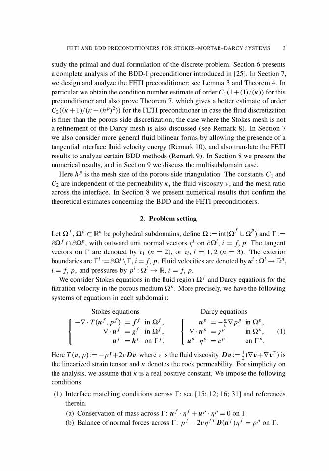
have the following matrix representation of the coupled problem in (11):
A fI I B f T
I I A f T0 I 0 0 0 0 0 0
B fI I 0 B f T
0 I 0 0 0 0 0 0
A f0 I B f T
I0 A f00 B f T 0 0 0 0 C f T
0 0 B f 0 0 0 0 0 0
0 0 0 0 ApI I B pT
I I ApT0 I 0 0
0 0 0 0 B pI I 0 B p
I0 0 0
0 0 0 0 Ap0 I B pT
I0 Ap00 B pT
−C pT
0 0 0 0 0 0 B p 0 0
0 0 C f 0 0 0 −C p 0 0
u fI
p fI
u f0
p f
upI
p pI
u p0
p p
λ
=
f fI
g fI
f f0
g f
f pI
g pI
f p0
g p
0
. (13)
Following [19; 40], we choose the following matrix representation in each sub-domain �i , i = f, p:
AiI I BiT
I I AiT0 I 0
BiI I 0 Bi
I0 0
Ai0 I BiT
I0 Ai00 BiT
0 0 Bi 0
=[
K iI I K iT
0 I
K i0 I K i
00
]. (14)
5.1. The primal formulation. From the last equation in (13) we see that the mortarcondition on 0 (using the Darcy side as the slave side) can be imposed as u p
0 =
(C p)−1C f u f0 =5u f
0, where 5 is the L2(0) projection on the space of piecewiseconstant functions on each subinterval ep
∈ Tph p(0). We note that C p is a diagonal
matrix for the lowest order Raviart–Thomas elements.Now we eliminate ui
I , piI , i = f, p, and λ, to obtain the following (saddle point)
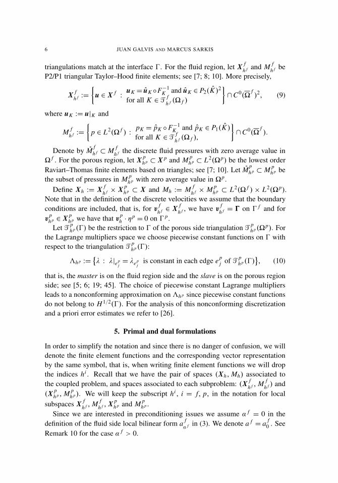
Schur complement:
S
u f0
p f
p p
=b0
b f
bp
. (15)
Here S is given by
S : =
S f0 B f T 0
B f 0 00 0 0
+ 5T
S p0 0 B pT
0 0 0B p 0 0
5= S f+ S p
=
S f0 +5
T S p05 B f T 5T B pT
B f 0 0B p5 0 0
= [S0 BT
B 0
],
FETI AND BDD PRECONDITIONERS FOR STOKES–MORTAR–DARCY SYSTEMS 9
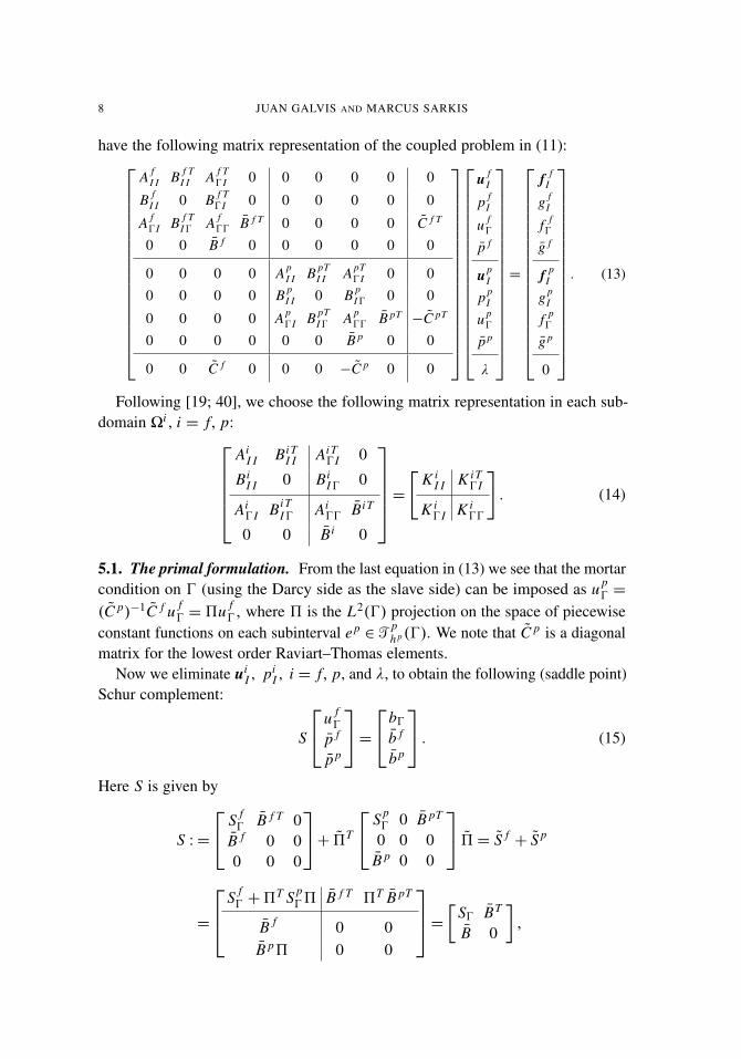
where
5 :=
5 0 00 1 00 0 1
and BT:= [B f T 5T B pT
]. (16)
Here, we have introduced
S f:=
S f0 B f T 0
B f 0 00 0 0
, S p:= 5T
S p0 0 B pT
0 0 0B p 0 0
5 (17)
and
S0 := S f0 +5
T S p05. (18)
The local matrices Si0 and Bi and the local Schur complement Si are given by
Si=
[Si0 BiT
Bi 0
]:= K i
00 − K i0 I(K i
I I)−1K iT
0 I , i = p, f. (19)
The right side of (15) is given byb0b f
bp
= f f
0
g f
0
−K f
0 I
(K f
I I
)−1
[f f
I
g fI
]0
+
5
T f p0
0g p
− 5T
K p0 I
(K p
I I
)−1
[f p
I
g pI
]0
.
We note that the reduced system (15), as well as the original system (13), issolvable when b f
+ bp= 0, and the solution is unique when we restrict to pressures
with zero average value on �.From now on we only work with functions defined on 0 and extended inside
the subdomain using the discrete Stokes and Darcy problems. It is convenient todefine the space
V0 :={v0 = (v
f0, v
p0) : v
f0 = SH(v f
· η f|0) and v p
0 = DH(v p· ηp|0))
}(20)
and
Mh0 :=
{q ∈ Mh
: q i= piecewise constant in �i for i = f, p,
and∫� f
q f+
∫�p
q p= 0
}. (21)

10 JUAN GALVIS AND MARCUS SARKIS
Here SH (DH) is the velocity component of the discrete Stokes (Darcy) harmonicextension operator that maps discrete interface normal velocity u f
0 ∈ H 1/200 (0) (re-
spectively u p0 ∈ (H
1/2(0))′) to the solution of following problem: Find ui∈ X i
hi
and pi∈ M
ihi such that for all vi
∈ X ihi and q i
∈ Mihi , i = f, p, we have
a f (SHu f , v f )+ b f (v f , p f ) = 0,b f (SHu f , q f ) = 0,
SHu f· η f= u f
0 on 0,SHu f
= 0 on 0 f ,
(22)
and a p(DHu p, v p)+ bp(v p, p p) = 0,
bp(DHu p, q p) = 0,DHu p
· ηp= u p
0 on 0,DHu p
· ηp= 0 on 0 p.
(23)
The degrees of freedom associated with SHu f· τ f on 0 are free. This cor-
responds to imposing the natural boundary condition τ T D(SHu f )η f = 0 on 0which is the expression for interface condition of Beavers–Joseph–Saffman withα f= 0.
For i = f, p, define the normal trace component of X ihi by
Z ihi =
{vi· ηi|0 : vi
∈ X ihi
}. (24)
Associated with the coupled problem (13) we introduce the balanced subspace:
V0,B :={v f0 ∈ Z f
h f : (vf0,5v
f0 ) ∈ V0 and
∫0
v f0 · η f = 0
}, (25)
with V0 defined in (20); see [40]. Observe that V0,B = KerB, where B is definedin (16) and (19). Then for v f
0 ∈ V0,B we have Bv f0 = 0. We will refer to functions
vf0 ∈ V0,B as balanced functions. If v p
0 =5vf0 and v f
0 is a balanced function, thenwe also say that v p
0 is a balanced function or the pair (v f0 ,5v
f0) is balanced.
5.2. Dual formulation. In the system (13), we first eliminate the unknowns u fI , p f
Iand up
I , p pI . We obtain
S f0 B f T 0 0 C f T
B f 0 0 0 0
0 0 S p0 B pT
−C pT
0 0 B p 0 0
C f 0 −C p 0 0
u f0
p f
u p0
p p
λ
=
b f
bp
0
, (26)

FETI AND BDD PRECONDITIONERS FOR STOKES–MORTAR–DARCY SYSTEMS 11
where the right side of (26) is given by
b f
bp
0
=
[f f0
g f
]− K f
0 I
(K f
I I
)−1[
f fI
g fI
][
f p0
g p
]− K p
0 I
(K p
I I
)−1
[f p
I
g pI
]0
.
Here Si0, K i
I I and K iI0, i = f, p, are defined in (19) and (14).
Let Ni :=[C i 0
]and consider Si , i = f, p, defined in (19). Then the matrix in
the left side of (26) can be rewritten asS f 0 N f T
0 S p−N pT
N f−N p 0
.Now we eliminate the unknowns u f
0, p f and u p0, p p. We end up with the reduced
systemFλ= c, (27)
where the operator F is defined by
F := N f (S f )−1 N f T+ N p(S p)−1 N pT , (28)
and the right side c is given by
c = N f (S f )−1
{[f f0
g f
]− K f
0 I
(K f
I I
)−1
[f f
I
g fI
]}
− N p(S p)−1
{[f p0
g p
]− K p
0 I
(K p
I I
)−1
[f f
Ig p
I
]}.
Note that F is positive semidefinite and since a discrete Lagrange multiplier in3h p does not have necessarily zero mean average value on 0, the operator F hasone simple zero eigenvalue corresponding to a constant Lagrange multiplier. Thelinear system above, as well as the original linear system (13), is solvable for zeromean right side, that is, for cT
· (1, . . . , 1)= 0.
6. BDD preconditioner
In this section we design and analyze a BDD type preconditioner for the Schurcomplement system (15); see [9; 19; 42] and also [1; 21; 35; 40; 43]. For the sake
12 JUAN GALVIS AND MARCUS SARKIS
of simplicity on the analysis we assume that 0 = {1}× (0, 1), � f= (1, 2)× (0, 1)
and�p= (0, 1)×(0, 1). We introduce the velocity coarse space on 0 as the span of
the normal velocity v0 = y(1− y) (with v0 also denoting its vector representation).Define
R0 :=
[vT
0 00 I2×2
], S0 := R0S RT
0 and Q0 := RT0 S†
0 R0. (29)
The system (15) is solvable when the right side satisfies b f+ bp
= 0 withuniqueness of the solution in the space of vectors with pressure component havingzero average value on �. Then S0 is invertible restricted to vectors with pressurecomponent in Mh
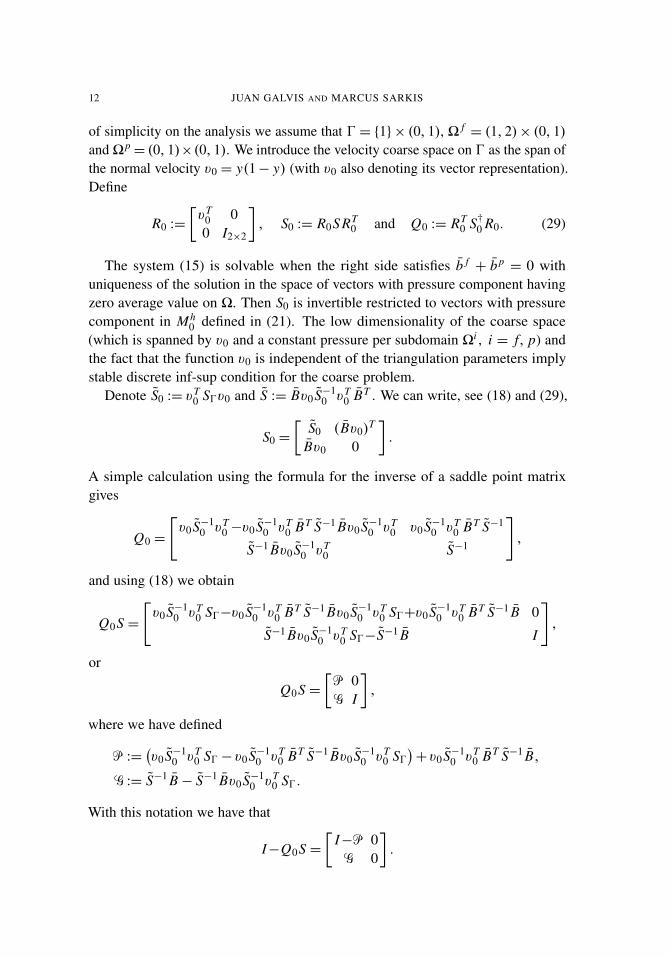
0 defined in (21). The low dimensionality of the coarse space(which is spanned by v0 and a constant pressure per subdomain �i , i = f, p) andthe fact that the function v0 is independent of the triangulation parameters implystable discrete inf-sup condition for the coarse problem.
Denote S0 := vT0 S0v0 and S := Bv0 S−1
0 vT0 BT . We can write, see (18) and (29),
S0 =
[S0 (Bv0)
T
Bv0 0
].
A simple calculation using the formula for the inverse of a saddle point matrixgives
Q0 =
[v0 S−1
0 vT0 −v0 S−1
0 vT0 BT S−1 Bv0 S−1
0 vT0 v0 S−1
0 vT0 BT S−1
S−1 Bv0 S−10 vT
0 S−1
],
and using (18) we obtain
Q0S =
[v0 S−1
0 vT0 S0−v0 S−1
0 vT0 BT S−1 Bv0 S−1
0 vT0 S0+v0 S−1
0 vT0 BT S−1 B 0
S−1 Bv0 S−10 vT
0 S0−S−1 B I
],
or
Q0S =[
P 0G I
],
where we have defined
P :=(v0 S−1
0 vT0 S0 − v0 S−1
0 vT0 BT S−1 Bv0 S−1
0 vT0 S0
)+ v0 S−1
0 vT0 BT S−1 B,
G := S−1 B− S−1 Bv0 S−10 vT
0 S0.
With this notation we have that
I−Q0S =[
I−P 0G 0
].
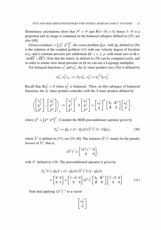
FETI AND BDD PRECONDITIONERS FOR STOKES–MORTAR–DARCY SYSTEMS 13
Elementary calculations show that P2= P and B(I−P) = 0, hence I−P is a
projection and its image is contained on the balanced subspace defined in (25); seealso [40].
Given a residual r =[
f T0 gT
]T , the coarse problem Q0r , with Q0 defined in (29),is the solution of the coupled problem (13) with one velocity degree of freedom(v0), and a constant pressure per subdomain �i , i = f, p, with mean zero in �=int(�
f∪�p). Note that the matrix S0 defined in (29) can be computed easily, and
in order to ensure zero mean pressure on � we can use a Lagrange multiplier.For balanced functions v f
0 and u f0 , the S0-inner product (see (18)) is defined by
〈u f0, v
f0 〉S0 := 〈S0u f
0, vf0 〉 = u f T
0 S0vf0 .
Recall that Bu f0 = 0 when u f
0 is balanced. Then, on this subspace of balancedfunctions, the S0 inner product coincides with the S-inner product defined by
⟨v f0
q f
q p
,u f
0
p f
p p
⟩S
:=
v f0
q f
q p
T
S
u f0
p f
p p
= [v f0
q
]T [S0 BT
B 0
][u f0
p
],
where pT=[
p p p p]T . Consider the BDD preconditioner operator given by
S−1N := Q0+ (I−Q0S) (S f )† (I−SQ0) , (30)
where S f is defined in (17); see [19; 40]. The notation (S f )† stands for the pseudo-inverse of S f , that is,
(S f )† =
[(S f )−1 0
0 0
],
with S f defined in (19). The preconditioned operator is given by
S−1N S = Q0S+ (I−Q0S) (S f )†S (I−Q0S)
=
[P 0G I
]+
[I−P 0
G 0
](S f )†
[S0 BT
B 0
] [I−P 0
G 0
]. (31)
Note that applying (S f )−1 to a vector[u f0
p
]

14 JUAN GALVIS AND MARCUS SARKIS
is equivalent to solving the linear systemA f
I I B f TI I A f T
0 I 0
B fI I 0 B f
I0 0
A f0 I B f T
I0 A f00 B f T
0 0 B f 0
w
fI
s fI
wf0
s f
=
00
u f0
p f
.
If u f0 is balanced, so is the velocity component of
(S f )−1
[u f0
p f
].
Using elementary calculations with the matrices in (31) we obtain⟨S−1
N S[ u0
p
],[ v0
q
]⟩S= 〈(S f
0 )−1S0u0, v0〉S0 ,
for u0, v0 ∈ Range(I−P). In order to bound the condition number of the pre-conditioned operator S−1
N S, we need only analyze the condition of the operator(S f0 )−1S0. Note that
c〈u f0, u f
0〉S0 ≤⟨(
S f )−1S0u f
0, u f0
⟩S0≤ C〈u f
0, u f0〉S0
is equivalent to
c〈S f u f0, u f
0〉 ≤ 〈S0u f0, u f
0〉 ≤ C〈S f u f0, u f
0〉. (32)
The next theorem shows that the condition number estimate for the BDD methodintroduced in (30) is of order O(1+ (1/κ)), where κ is the permeability of theporous medium; see (1).
Theorem 2. If u f0 is a balanced function then
〈S f0 u f
0, u f0〉 ≤ 〈S0u f
0, u f0〉 ≺
(1+ 1
κ
)〈S f0 u f
0, u f0〉.
Proof. The lower bound follows trivially from S f0 and S p
0 being positive on thesubspace of balanced functions. Next we concentrate on the upper bound.
Let v f0 be a balanced function and v p
0 = 5vf0 . Define v p
= DHvp0 ; see (23).
Using properties of the discrete operator DH [38] we obtain
〈S p0v
p0, v
p0〉 = a p(v p, v p)�
ν
κ‖v
p0‖
2(H1/2)′(0).
Using the L2-stability property of mortar projection 5, we have
‖vp0‖
2(H1/2)′(0) ≺ ‖v
p0‖
2L2(0) = ‖v
f0‖
2L2(0) ≺ ‖v
f0‖
2H1/2
00 (0).

FETI AND BDD PRECONDITIONERS FOR STOKES–MORTAR–DARCY SYSTEMS 15
With SH defined in (22), define v f= SHv
f0 . Using properties of SH [40], we
haveν‖v
f0‖
2H1/2
00 (0)� a f (v f , v f )
and then〈S p0v
p0, v
p0〉 ≺
1κ〈S f u f
0, u f0〉. (33)
This gives the upper bound and finishes the proof. �
Recall that we consider the preconditioned projected conjugate gradient methodapplied to the Schur complement problem (15). Here is the algorithm:
(1) Initialize
x (0) = Q0b+w
d(0) = b− Sx (0)
with w ∈ Range(I−Q0S). Recall that all vectors have three components,for instance,
x =
x0x f
x p
and b =
b0b f
bp
.(2) Iterate k = 1, 2, . . . until convergence
Precondition: z(k−1)= (S f )†d(k−1),
Project: y(k−1)= (I−Q0S)z(k−1)
βk= 〈y(k−1), d(k−1)
〉/〈y(k−2), d(k−1)〉 [β(1) = 0] ,
r (k) = y(k−1)+β(k)r (k) [r (1) = y(0)] ,
α(k) = 〈y(k−1), d(k−1)〉/〈d(k), Sr (k)〉,
x (k) = x (k−1)+α(k)r (k),
d(k) = d(k−1)−α(k)Sr (k).
Implementation of the projected preconditioned conjugate gradient algorithm for thesystem (15) involving the BDD preconditioner (30).
7. FETI preconditioner
In this section we analyze a FETI preconditioner for the reduced linear system(27); see [9; 19; 42; 24; 30; 37]. Recall the definition of F in (28). We proposethe following preconditioner
(N p)†(S p)(N p)†T , (34)
where (N p)† is the pseudo-inverse (N p)† = [(C p)−1 0].

16 JUAN GALVIS AND MARCUS SARKIS
Note that after computing the action of (S f )−1 and (S p)−1 in the application ofF to a zero average Lagrange multiplier, we end up with balanced functions. There-fore, to apply the preconditioned operator (N p)†(S p)(N p)†T F to a zero meanLagrange multiplier, we do not need to solve a coarse problem at the beginning ofthe CG, nor inside of the CG iteration.
The FETI preconditioner in (34) can be considered as the dual preconditionerof the BDD preconditioner defined in (30); see the proof of Lemma 3 below.
Recall the definition of Si , i = f, p, in (19) and the definition of space ofbalanced functions V0 = V f
0 × V p0 in (25) and (24). We prove the following result.
Lemma 3. Let λ ∈3h p ∩ L20(0) be a zero mean Lagrange multiplier. Then
〈N f (S f )−1 N f Tλ, λ〉 ≺1κ〈N p(S p)−1 N pTλ, λ〉.
Proof. Consider a zero mean Lagrange multiplier λ. Define t = (S p0)−1/2C pTλ and
w f= C f Tλ. Then it is enough to prove that
‖(S f0 )−1/2w f
‖2≺ ‖t‖2.
Since w f is balanced, that is, w f∈ V f
0 , we have that
‖(S f0 )−1/2w f
‖2= sup
z f ∈Z fh f
〈(S f0 )−1/2w f , z f
〉2
‖z f ‖2= supv f balanced
〈w f , v f〉
2
‖(S f0 )
1/2v f‖2
= supv f balanced
〈λ, N f v f〉
2
‖(S f0 )
1/2v f‖2
= supv f balanced
〈(S p0)−1/2C pλ, (S p
0)1/2(C p)−1C f v f
〉2
‖(S f0 )
1/2v f‖2.
Then using the Cauchy–Schwarz inequality and (33) in the proof of Theorem 2,we have
‖(S f0 )−1/2w f
‖2= supv f balanced
〈t, (S p0)
1/2(C p)−1C f v f〉
2
‖(S f0 )
1/2v f‖2
≤ ‖t‖2 supv f balanced
‖(S p0)
1/2(C p)−1C f v f‖
2
‖(S f0 )
1/2v f‖2≺
1κ‖t‖2. �
Using Lemma 3 we can derive the following estimate for the condition numberof the FETI preconditioner defined in (34).
Theorem 4. Let λ be a zero mean Lagrange multiplier. Then
〈N p(S p)−1 N Tp λ, λ〉 ≺ 〈Fλ, λ〉 ≺
(1+ 1
κ
)〈N p(S p)−1 N pTλ, λ〉.

FETI AND BDD PRECONDITIONERS FOR STOKES–MORTAR–DARCY SYSTEMS 17
The condition number estimate O((κ+1)/κ) can be improved in the case wherethe fluid side triangulation is finer than the porous side triangulation. This case hassome advantages when κ is small. In order to fix ideas and simplify notation weanalyze in detail the case where the triangulation of the fluid side is a refinementof the porous side triangulation. In particular, in Theorem 7, we will prove that thecondition of the FETI preconditioned operator is of order O((κ + 1)/(κ + (h p)2))
in this simpler situation. The analysis that we will present to prove Theorem 7 canbe extended easily for the case where the fluid side triangulation is finer than (andnot necessarily a refinement of) the porous side triangulation; see Remark 8.
We assume that the fluid side discretization on 0, Tfh f (�
f )|0, is a refinementof the corresponding porous side discretization, T
ph p(�p)|0. That is, assume that
h p= rh f for some positive integer r . We will refer to this assumption as the
nested refinement assumption. For j = 1, . . . ,m p, we introduce the normal fluidvelocity φ f
j as the P2 bubble function defined on Tph p(�p)|0 and with support on
the interval epj = {0} × [( j − 1)h p, jh p
]. Recall that we are using P2/P1 Taylor–Hood discretization on the fluid side. Under the nested refinement assumption wehave φ f
j ∈ Z fh f with Z f
h f defined in (24). Denote by Z fh f ,b the subspace of Z f
h f
spanned by all φ fj , j = 1, . . . ,m p, and by Z f
h f ,0 the subspace of Z fh f spanned by
functions with zero average on all edges epj , j = 1, . . . ,m p. Note that Z f
h f ,b andZ f
h f ,0 form a direct sum for Z fh f and the image 5Z f
h f ,0 is the zero vector.Before deriving the condition number estimate of the FETI preconditioner under
the nested refinement assumption we first prove a preliminary lemma.
Lemma 5. Assume that h p= rh f , where r is a positive integer. If v f
0,b ∈ Z fh f ,b is a
balanced function, then
〈S f0 v
f0,b, v
f0,b〉 ≺
κ
(h p)2〈S p05v
f0,b,5v
f0,b〉.
Proof. Let
vf0,b =
m p∑j=1
β jφfj ∈ Z f
h f ,b ⊂ Z fh f ,
and note that since the basis functions φ fj , j = 1, . . . ,m p, do not overlap each
other on 0, they are orthogonal in L2(0) and also in H 10 (0). Then
‖vf0,b‖
2L2(0) =
m p∑j=1
β2j ‖φ
fj ‖
2L2(0) � h p
m p∑j=1
β2j , (35)
|vf0,b|
2H1(0) =
m p∑j=1
β2j |φ
fj |
2H1
0 (epj )�
1h p
m p∑j=1
β2j . (36)

18 JUAN GALVIS AND MARCUS SARKIS
Using (35), (36) and a interpolation estimate we see that
‖vf0,b‖
2H1/2
00 (0)�
m p∑j=1
β2j �
1h p ‖v
f0,b‖
2L2(0).
Note also that 〈S f vf0,b, v
f0,b〉 ≤ a f (SHv
f0,b,SHv
f0,b)� ν‖v
f0,b‖
2H1/2
00 (0).
Denote by
z p0,b =
m p∑j=1
ρ jχepj
the unique piecewise constant function such that5v f0,b= z p
0,b. Note that |ρ j |� |β j |,j = 1, . . . ,m p. We obtain
〈S f0 v
f0,b, v
f0,b〉 ≺
ν
h p ‖vf0,b‖
2L2(0) �
ν
h p ‖zp0,b‖
2L2(0) (37)
≺ν
(h p)2‖z p0,b‖
2(H1/2)′(0) �
κ
(h p)2〈S p0 z p0,b, z p
0,b〉, (38)
where we have used an inverse inequality for piecewise constant functions. �
We now translate Lemma 5 in a result concerning the dual preconditioner.
Lemma 6. Assume that h p= rh f , where r is a positive integer and let λ be a zero
mean Lagrange multiplier. Then
(h p)2
κ〈N p(S p)−1 N pTλ, λ〉 ≺ 〈N f (S f )−1 N f Tλ, λ〉.
Proof. We proceed as before. Let t = (S f0 )−
12 C f Tλ and w = C pλ. Then
‖(S p0)−
12w‖2 = sup
z p∈Z ph p
〈(S p0)−
12w, z p
〉2
‖z p‖2= supv pbalanced
〈w, v p〉
2
‖(S p0)
12 v p‖2
= supv pbalanced
〈λ, N pv p〉
2
‖(S p0)
12 v p‖2
= supv
fb balanced
〈λ, C f vfb 〉
2
‖(S p0)
12 (C p)−1 N f v
fb‖
2
= supv
fb balanced
〈(S f0 )−
12 C f Tλ, (S f
0 )12 v
fb 〉
2
‖(S p0)
12 (C p)−1C f v
fb‖
2
≤ ‖t‖2 supv
fb balanced
‖(S f0 )
12 v
fb‖
2
‖(S p0)
12 (C p)−1C f v
fb‖
2≺
κ
(h p)2‖t‖2,
where the last step follows from Lemma 5. �
From Lemmas 3 and 6, the next theorem follows.

FETI AND BDD PRECONDITIONERS FOR STOKES–MORTAR–DARCY SYSTEMS 19
Theorem 7. Assume that h p= rh f , where r is a positive integer. Let λ be a zero
mean Lagrange multiplier, then(1+
(h p)2
κ
)〈N p(S p)−1 N pTλ, λ〉 ≺ 〈Fλ, λ〉 ≺
(1+
1κ
)〈N p(S p)−1 N pTλ, λ〉.
We solve the system (27) using preconditioned conjugate gradient. Here is thealgorithm:
(1) Initialize:
x (0) = 0 (no coarse problem)
λ(0) = c
(2) Iterate k = 1, 2, . . . until convergence:
Precondition: y(k−1)= (N p)†(S p)(N pT )†d(k−1),
βk= 〈y(k−1), d(k−1)
〉/〈y(k−2), d(k−1)〉 [β(1) = 0] ,
r (k) = y(k−1)+β(k)r (k) [r (1) = y(0)] ,
α(k) = 〈y(k−1), d(k−1)〉/〈d(k), Fr (k)〉,
x (k) = x (k−1)+α(k)r (k),
d(k) = d(k−1)−α(k)Fr (k).
Implementation of the preconditioned conjugate gradient algorithm for the system (27)involving the FETI preconditioner (34).
Remark 8. Theorem 7 can be extended for the case where h f≤ 2h p. We only
need to extend the argument given in the proof of Lemma 5. The basic idea inthe proof of Lemma 5 is to associate a bubble function φ f
j ∈ Z fh f to each porous
side element epj , j = 1, . . . ,m p, in such a way that we can construct a one to
one and continuous map v f0,b 7→ z p
0,b. The bubble functions φ fj , j = 1, . . . ,m p,
can be chosen orthogonal in L2(0) and in H 10 (0). This can also be done when
h f≤ h p. The smaller the h f , the closer is the size of the support of the bubble φ f
j
to the size of the element epj since more and more elements e f can be associated
to only one element ep. This construction can also be carried out in the caseh p < h f
≤ 2h p where nonorthogonal Taylor–Hood basis functions must be used.This last situation leads to the appearance of an additional constant that dependson the nonorthogonality; see Section 8.
Remark 9. We note that Lemma 5 can be used directly to obtain a bound for thebalancing domain decomposition preconditioner similar to the one presented inSection 6 but with S p instead of S f in (30); see Proposition 2 of [25]. In this casean additional variable elimination is needed. We have to eliminate the component

20 JUAN GALVIS AND MARCUS SARKIS
of the normal fluid velocity in the space Z fh f ,0 and work with the Schur comple-
ment with respect to the space Z fh f ,b. This is rather difficult to implement (we can
use Lagrange multipliers in this case). Then passing to the dual preconditionerpermits us to take advantage of the case where the fluid side discretization on 0 isa refinement of the corresponding porous side discretization.
Remark 10. Theorems 2, 4 and 7 are also valid for the case α f > 0 in (3). Tosee this we need to compare, for different values of α f , the energy of discreteextensions for a given normal velocity defined on 0. Given the outward normalvelocity v f
0 on 0, let SHα f vf0 denote the discrete harmonic extension in the sense of
(a fα f , b f ), that is, the solution of problem (22) with a f replaced by a f
α f . Recall thata f= a f
0 , where a f0 = aα f when α f
= 0, and therefore, SHvf0 =SH0v
f0 . Note that
in (22) we have imposed the natural boundary condition τ T D(SHu f )η f = 0 on 0.Now we define another extension denoted by SHv
f0 . Given the outward normal
velocity v f0 on 0, let SHv
f0 be the (a f , b f )-discrete harmonic extension given
by the solution of (22) with the boundary condition SHvf0 · τ = 0. For both SH
and SH are imposed essential boundary condition v f0 for the normal component
on 0. The difference between them is in how the boundary condition is imposedfor the tangential component on 0: For the SH, is imposed homogeneous naturalboundary condition, while for SH, is imposed homogeneous essential boundarycondition.
Both extensions SHα f and SH satisfy the zero discrete divergence and boundaryconditions in (22). Using this fact and the minimization property of the (a f
α f , b f )-discrete harmonic extension SHα f and the (a f , b f )-discrete harmonic extensionSH, we get
a f (SHvf0 ,SHv
f0 )
= a f0 (SHv
f0 ,SHv
f0 ) (by definition)
≤ a f0 (SHα f v
f0 ,SHα f v
f0 ) (by the minimization property of SH)
≤ a fα f (SHα f v
f0 ,SHα f v
f0 ) (α f > 0)
≤ a fα f (SHv
f0 , SHv
f0 ) (by the minimization property of SHα f )
= a f0 (SH0v
f0 , SH0v
f0 ) (because SHu f
· τ f= 0 on 0)
� ν‖vf0‖
2H1/2
00 (0)
� a f (SH0vf0 ,SHv
f0 ).
The last two equivalences follow from properties of the (a f , b)-discrete harmonicextensions SH and SH (which coincides with the discrete Stokes harmonic ex-tension) [28; 40]. The two equivalences appearing above are independent of the

FETI AND BDD PRECONDITIONERS FOR STOKES–MORTAR–DARCY SYSTEMS 21
permeability, fluid viscosity and mesh sizes. Then, the energy of the (a fα f , b)-
discrete harmonic extensions is equivalent to the energy of the (a f , b)-discreteharmonic extension, that is, the discrete Stokes harmonic extension. This equiva-lence guarantees the extensions of Theorems 2, 4 and 7 to the case α f > 0.
8. Numerical results
In this section we present numerical tests in order to verify the estimates in Theo-rems 2, 4 and 7. We consider� f
= (1, 2)×(0, 1) and�p= (0, 1)×(0, 1). See [11]
and [26] for examples of exact solutions and compatible divergence and boundarydata. Note that the reduced systems (15) and (27) involve only degrees of freedomon the interface 0. To solve both reduced systems (15) and (27) we can use thePCG algorithms described on pages 15 and 19. Recall that the original system(11) is a “three times” saddle point problem. Note that since the finite elementbasis of M f
h f ×M ph p and 3h p
have no zero mean, the finite element matrix in (13)has the kernel composed by constant pressures in �= int(� f ∪�p) and constantLagrange multipliers on 0. The corresponding system is solved up to a constantpressure and a constant Lagrange multiplier. These constants can be recoveredwhen imposing the zero average pressure constraint [26].
In our test problems we compute the eigenvalues of the preconditioned operators.We also run PCG until the initial residual is reduced by a factor of 10−6.
8.1. BDD preconditioner. In the case of the BDD preconditioner (30) for (15), wesolve a coarse problem before reducing the system to ensure balanced velocities atthe beginning of the CG iterations.
We consider α f= 0 and ν = 1, and different values of h f and h p with non-
matching grids across the interface 0. Table 1 shows results for κ = 1, Table 2for κ = 10−3 and Table 3 for κ = 10−5. These three tables reveal growth of orderO(1+ (1/κ)) in κ and hence, verify the sharpness of the estimate in Theorem 2.
h f↓ h p
→ 3−1∗ 2−0 3−1
∗ 2−1 3−1∗ 2−2 3−1
∗ 2−3 3−1∗ 2−4
2−1∗ 2−0 1, 1.0189(3) 1, 1.0198(3) 1, 1.0194(3) 1, 1.0193(3) 1, 1.0193(3)
2−1∗ 2−1 1, 1.0209(3) 1, 1.0200(3) 1, 1.0197(3) 1, 1.0196(3) 1, 1.0196(3)
2−1∗ 2−2 1, 1.0217(3) 1, 1.0205(3) 1, 1.0202(3) 1, 1.0201(3) 1, 1.0201(3)
2−1∗ 2−3 1, 1.0220(3) 1, 1.0208(3) 1, 1.0204(3) 1, 1.0203(3) 1, 1.0203(3)
2−1∗ 2−4 1, 1.0221(3) 1, 1.0209(3) 1, 1.0205(3) 1, 1.0204(3) 1, 1.0204(3)
Table 1. Minimum and maximum eigenvalues (and number ofPCG iterations) for the BDD preconditioned operator. Here κ = 1and α f
= 0.

22 JUAN GALVIS AND MARCUS SARKIS
h f↓ h p
→ 3−1∗ 2−1 3−1
∗ 2−2 3−1∗ 2−3 3−1
∗ 2−4
2−1∗ 2−0 1, 21.0147(3) 1, 20.6035(3) 1, 20.3686(3) 1, 20.2893(3)
2−1∗ 2−1 1, 21.3303(6) 1, 20.8549(7) 1, 20.6550(7) 1, 20.5836(7)
2−1∗ 2−2 1, 22.0017(6) 1, 21.3392(9) 1, 21.1424(10) 1, 21.0735(10)
2−1∗ 2−3 1, 22.2367(6) 1, 21.6045(10) 1, 21.3626(9) 1, 21.2955(10)
2−1∗ 2−4 1, 22.3479(6) 1, 21.7006(10) 1, 21.4666(11) 1, 21.3929(9)
Table 2. Minimum and maximum eigenvalues (and number ofPCG iterations) for the BDD preconditioned operator. Here κ =10−3 and α f
= 0.
h f↓ h p
→ 3−1∗ 2−1 3−1
∗ 2−2 3−1∗ 2−3 3−1
∗ 2−4
2−1∗ 2−0 1, 1977.08(3) 1, 1945.05(3) 1, 1932.10(3) 1, 1928.32(3)
2−1∗ 2−1 1, 1997.27(6) 1, 1972.77(7) 1, 1961.34(7) 1, 1957.88(7)
2−1∗ 2−2 1, 2053.57(6) 1, 2021.03(13) 1, 2010.27(17) 1, 2006.90(17)
2−1∗ 2−3 1, 2079.68(6) 1, 2044.05(13) 1, 2032.42(21) 1, 2029.13(31)
2−1∗ 2−4 1, 2090.10(6) 1, 2054.33(13) 1, 2042.26(22) 1, 2038.90(28)
Table 3. Minimum and maximum eigenvalues (and number ofPCG iterations) for the BDD preconditioned operator. Here κ =10−5 and α f
= 0.
8.2. FETI preconditioner. In the case of the FETI preconditioner (34), we solvethe reduced system (27) up to a constant Lagrange multiplier and a constant pres-sure. These constants are recovered after enforcing zero mean pressure on � =int (�
f∪�
p) [26]. We recall that the FETI method can be viewed as the dual
preconditioner counterpart of the BDD preconditioner. We repeat the same exper-iments mentioned above for the latter preconditioner.
h f↓ h p
→ 3−1∗ 2−1 3−1
∗ 2−2 3−1∗ 2−3 3−1
∗ 2−4
2−1∗ 2−0 1.0000, 1.0208(3) 1.0000, 1.0194(3) 1.0000, 1.0193(3) 1.0000, 1.0193(3)
2−1∗ 2−1 1.0017, 1.0200(3) 1.0000, 1.0197(3) 1.0000, 1.0196(3) 1.0000, 1.0196(3)
2−1∗ 2−2 1.0026, 1.0205(3) 1.0004, 1.0202(3) 1.0000, 1.0200(3) 1.0000, 1.0201(3)
2−1∗ 2−3 1.0027, 1.0208(3) 1.0007, 1.0204(3) 1.0001, 1.0203(3) 1.0000, 1.0203(3)
2−1∗ 2−4 1.0028, 1.0209(2) 1.0007, 1.0205(3) 1.0002, 1.0204(3) 1.0000, 1.0204(3)
2−1∗ 2−5 1.0028, 1.0209(2) 1.0007, 1.0206(3) 1.0002, 1.0205(3) 1.0000, 1.0204(3)
Table 4. Minimum and maximum eigenvalues (and number ofPCG iterations) of the FETI preconditioned operator. Here κ = 1and α f
= 0.

FETI AND BDD PRECONDITIONERS FOR STOKES–MORTAR–DARCY SYSTEMS 23
h f ↓ h p→ 3−1∗ 2−1 3−1
∗ 2−2 3−1∗ 2−3 3−1
∗ 2−4
2−1∗ 2−0 1.000, 20.7608(3) 1.000, 20.4405(3) 1.000, 20.3110(3) 1.000, 20.2732(3)
2−1∗ 2−1 2.707, 20.9627(5) 1.000, 20.7177(7) 1.000, 20.6034(7) 1.000, 20.5688(7)
2−1∗ 2−2 3.634, 21.5257(5) 1.425, 21.2003(10) 1.000, 21.0927(12) 1.000, 21.0590(12)
2−1∗ 2−3 3.714, 21.7868(5) 1.651, 21.4305(9) 1.106, 21.3142(11) 1.000, 21.2813(12)
2−1∗ 2−4 3.760, 21.891 (5) 1.663, 21.5333(9) 1.162, 21.4126(11) 1.026, 21.3790(12)
2−1∗ 2−5 3.771, 21.937 (5) 1.673, 21.5768(9) 1.164, 21.4561(11) 1.040, 21.4220(12)
Table 5. Minimum and maximum eigenvalues (and number ofPCG iterations) for the FETI preconditioned operator. Here κ =10−3 and α f
= 0.
h f↓ h p
→ 3−1∗ 2−2 3−1
∗ 2−3 3−1∗ 2−4
2−1∗ 2−0 1.00, 1945.05(3) 1.00, 1932.10(3) 1.00, 1928.32(3)
2−1∗ 2−1 1.00, 1972.77(7) 1.00, 1961.34(7) 1.00, 1957.88(7)
2−1∗ 2−2 43.45, 2021.03(11) 1.00, 2010.27(17) 1.00, 2006.90(17)
2−1∗ 2−3 66.10, 2044.05(11) 11.58, 2032.42(20) 1.00, 2029.13(37)
2−1∗ 2−4 67.29, 2054.33(10) 17.20, 2042.26(19) 3.64, 2038.90(35)
2−1∗ 2−5 68.32, 2058.68(10) 17.42, 2046.61(10) 5.04, 2043.20(36)
Table 6. Minimum and maximum eigenvalues (and number ofPCG iterations) for the FETI preconditioned operator. Here κ =10−5 and α f
= 0.
We consider α f= 0, ν = 1 and different values of h f and h p with nonmatching
grids across the interface 0; see Table 4 on the previous page for the results whenκ = 1, Table 5 for κ = 10−3 and Table 6 for the case κ = 10−5. Note that in Tables4–6 the minimum eigenvalues are strictly greater than one when h f
≤ 2h p, andthe value of the minimum eigenvalues seem to stabilize very quickly for smallerh f with fixed h p. This confirms the extension of Theorem 7 for the case whereh f≤ 2h p (Remark 8). In Table 7 we present the numerical results where one of
the meshes on the interface is a refinement of the other side triangulation on theinterface. We observe a behavior similar to the behavior of Table 6 with a biggervalue for the minimum eigenvalue when h f ≤ h p. This verifies the estimates ofTheorem 7. This shows that the FETI preconditioner is scalable for the parametersfaced in practice, that is, when the fluid side mesh is finer than the porous side mesh,and the permeability κ is very small. We conclude that the numerical experimentsconcerning the FETI preconditioner reveal the sharpness of the results obtained inTheorems 4 and 7 and Remark 8.
Recall that we have assumed α f= 0. Now consider α f > 0. Numerical exper-
iment were performed with α f > 0 revealing results similar to the ones presented

24 JUAN GALVIS AND MARCUS SARKIS
h f↓ h p
→ 2−1∗ 2−2 2−1
∗ 2−3 2−1∗ 2−4
2−1∗ 2−0 1.00, 1961.35(3) 1.00, 1937.86(3) 1.00, 1929.93(3)
2−1∗ 2−1 1.00, 1986.49(7) 1.00, 1966.50(7) 1.00, 1959.36(7)
2−1∗ 2−2 176.56, 2034.92(7) 1.00, 2015.24(18) 1.00, 2008.35(17)
2−1∗ 2−3 151.62, 2061.45(7) 44.91, 2037.26(13) 1.00, 2030.55(45)
2−1∗ 2−4 154.45, 2071.06(7) 38.04, 2047.66(13) 11.98, 2040.29(21)
2−1∗ 2−5 154.86, 2075.43(7) 38.73, 2051.91(13) 10.20, 2044.66(24)
Table 7. Minimum and maximum eigenvalues (and number ofPCG iterations) for the FETI preconditioned operator. Here κ =10−5 and α f
= 0. The refinement condition of Theorem 7 is satis-fied under the diagonal.
h f↓ h p
→ 3−1 2−2 3−1 2−3 3−1 2−4
2−1 2−0 1.00, 1678.07(3) 1.00, 1666.84(3) 1.00, 1663.55(3)2−1 2−1 1.00, 1787.53(7) 1.00, 1776.50(7) 1.00, 1773.22(7)2−1 2−2 41.65, 1812.69(17) 1.00, 1801.61(17) 1.00, 1798.29(17)2−1 2−3 63.63, 1816.43(17) 11.24, 1804.66(13) 1.00, 1801.34(43)2−1 2−4 66.82, 1817.38(17) 16.75, 1805.30(13) 3.58, 1801.91(23)2−1 2−5 67.99, 1817.68(17) 17.37, 1805.57(13) 4.97, 1802.14(24)
Table 8. Minimum and maximum eigenvalues (and number ofPCG iterations) for the FETI preconditioned operator. Here κ =10−5 and α f
= 1.
above for the case α f= 0. We only include Table 8 which shows the extreme
eigenvalues of the FETI preconditioned operator for the case α f= 1, ν = 1 and
κ = 10−5. This table presents a similar behavior to the one with α f= 0 in Table
6 and hence confirms Remark 10, which says that the parameter α f does not playmuch of a role for preconditioning.
9. The multisubdomain case
The methods introduced in the previous sections considered only the two-subdo-main cases where discrete Stokes and Darcy indefinite subproblems are solvedexactly in each subdomain and in each CG iteration. These methods might be verycostly for large subproblems since direct or accurate iterative local solvers for theindefinite systems have to be used. In this section we show that the methodologydeveloped for the two-subdomain cases can be developed also for the multisub-domain case. The analysis (using tools developed in Section 7) and numericalexperiments for the multisubdomain case will be presented elsewhere.

FETI AND BDD PRECONDITIONERS FOR STOKES–MORTAR–DARCY SYSTEMS 25
We now extend the FETI method of Section 7 for many subdomains whenthe triangulations T
fh f and T
ph p coincide on the interface 0. Let {�i
j }ni
j=1 be ageometrically conforming substructures of �i , i = f, p. We also assume that{�
fj }
n f
j=1 ∪ {�pj }
n p
j=1 form a geometrically conforming decomposition of �; hence,the two decompositions are aligned on the interface 0. We define the local innerinterfaces as 0i
j = ∂�ij \ ∂�
i , j = 1, . . . , ni , i = f, p. We also define
0 =
n f⋃j=1
0fj ∪
n p⋃j=1
0pj ∪0.
See Figure 1. In order to simplify the presentation, we assume that for the fluidregion, the spaces X f
h f and M fh f are the P2/P0 triangular finite elements, while
for the porous region, the spaces X ph p ⊂ X p and M p
h p ⊂ L2(�p) are the lowestorder Raviart–Thomas finite elements based on triangles. Similar as in the previoussections, and using the FETI-DP framework [42], we decompose the velocity andpressure spaces as follows:
X fI : interior velocities in the subdomains {� f
j }n f
j=1
X f0
: interface velocities on 0 ∩�f
X pI : interior velocities in the subdomains {�p
j }n p
j=1
X p0
: interface velocities on 0 ∩�p
M iI , (i = p, f ): interior zero mean pressure in each subdomain {�i
j }ni
j=1, i = f, p
M i0, (i = p, f ): constant pressure in each subdomain {�i
j }ni
j=1, i = f, p
MI = M fI ×M p
I
X I = X fI × X p
I , X0 = X f0× X p
0, MI = M f
I ×M pI and M0 = M f
0 ×M p0
Figure 1. Global interface 0 that includes all local interfaces andthe Stokes–Darcy interface 0.
26 JUAN GALVIS AND MARCUS SARKIS
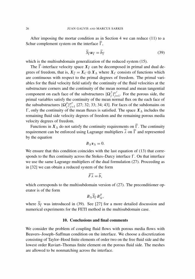
After imposing the mortar condition as in Section 4 we can reduce (11) to aSchur complement system on the interface 0,
S0u0 = b0 (39)
which is the multisubdomain generalization of the reduced system (15).The 0-interface velocity space X0 can be decomposed in primal and dual de-
grees of freedom, that is, X0 = XC ⊕ X1 where XC consists of functions whichare continuous with respect to the primal degrees of freedom. The primal vari-ables for the fluid velocity field satisfy the continuity of the fluid velocities at thesubstructure corners and the continuity of the mean normal and mean tangentialcomponent on each face of the substructures {� f
j }n f
j=1. For the porous side, theprimal variables satisfy the continuity of the mean normal flux on the each face ofthe subsubstructures {�p
j }n p
j=1 [27; 32; 33; 34; 43]. For faces of the subdomains on0, only the continuity of the mean fluxes is satisfied. The space X1 includes theremaining fluid side velocity degrees of freedom and the remaining porous mediavelocity degrees of freedom.
Functions in X1 do not satisfy the continuity requirements on 0. The continuityrequirement can be enforced using Lagrange multipliers λ on 0 and representedby the equation
B1v1 = 0.
We ensure that this condition coincides with the last equation of (13) that corre-sponds to the flux continuity across the Stokes–Darcy interface 0. On that interfacewe use the same Lagrange multipliers of the dual formulation (27). Proceeding asin [32] we can obtain a reduced system of the form
F λ= b,
which corresponds to the multisubdomain version of (27). The preconditioner op-erator is of the form
B1 S0BT1,
where S0 was introduced in (39). See [27] for a more detailed discussion andnumerical experiments for the FETI method in the multisubdomain case.
10. Conclusions and final comments
We consider the problem of coupling fluid flows with porous media flows withBeavers–Joseph–Saffman condition on the interface. We choose a discretizationconsisting of Taylor–Hood finite elements of order two on the free fluid side and thelowest order Raviart–Thomas finite element on the porous fluid side. The meshesare allowed to be nonmatching across the interface.

FETI AND BDD PRECONDITIONERS FOR STOKES–MORTAR–DARCY SYSTEMS 27
We design and analyze two preconditioners for the resulting symmetric linearsystem. We note that the original linear system is symmetric indefinite and involvesthree Lagrange multipliers: one for each subdomain pressure and a third one toimpose the weak conservation of mass across the interface 0; see Section 1.
One preconditioner is based on BDD methods and the other one is based onFETI methods. In the case of the BDD preconditioner, the energy is controlledby the Stokes side, while in the FETI preconditioner, the energy is controlled bythe Darcy system; see Theorems 2 and 4. In both cases a bound C1((κ + 1)/κ) isderived. Furthermore, under the assumption that the fluid side mesh on the inter-face is finer than the corresponding porous side mesh, we derive the better boundC2((κ + 1)/(κ + (h p)2)) for the FETI preconditioner; see Theorem 7 and Remark8. This better bound also shows that the FETI preconditioner is more scalable forparameters faced in practice, for example, problems with small permeability κ andwhere the fluid side mesh is finer than the porous side mesh. The constants C1
and C2 above are independent of the fluid viscosity ν, the mesh ratio across theinterface and the permeability κ .
References
[1] Y. Achdou, Y. Maday, and O. B. Widlund, Iterative substructuring preconditioners for mor-tar element methods in two dimensions, SIAM J. Numer. Anal. 36 (1999), no. 2, 551–580.MR 99m:65233 Zbl 0931.65110
[2] T. Arbogast and D. S. Brunson, A computational method for approximating a Darcy–Stokessystem governing a vuggy porous medium, Comput. Geosci. 11 (2007), no. 3, 207–218. MR2009b:76155 Zbl 05200264
[3] T. Arbogast and M. S. M. Gomez, A discretization and multigrid solvers for a Darcy–Stokessystem of three dimensional vuggy porous media, Comput. Geosci. 13 (2009), no. 3, 331–348.
[4] G. S. Beavers and D. D. Joseph, Boundary conditions at a naturally permeable wall, J. FluidMech. 30 (1967), 197–207.
[5] F. Ben Belgacem and Y. Maday, The mortar element method for three-dimensional finite ele-ments, RAIRO Modél. Math. Anal. Numér. 31 (1997), no. 2, 289–302. MR 98e:65107 Zbl0868.65082
[6] C. Bernardi, Y. Maday, and A. T. Patera, A new nonconforming approach to domain decomposi-tion: the mortar element method, Nonlinear partial differential equations and their applications.Collège de France Seminar, Vol. XI (H. Brezis et al., eds.), Pitman Res. Notes Math. Ser., no.299, Longman Sci. Tech., Harlow, 1994, pp. 13–51. MR 95a:65201 Zbl 0797.65094
[7] D. Braess, Finite elements: Theory, fast solvers, and applications in solid mechanics, 2nd ed.,Cambridge University Press, Cambridge, 2001. MR 2001k:65002 Zbl 0976.65099
[8] S. C. Brenner and L. R. Scott, The mathematical theory of finite element methods, Texts inApplied Mathematics, no. 15, Springer, New York, 1994. MR 95f:65001 Zbl 0804.65101
[9] S. C. Brenner and L.-Y. Sung, BDDC and FETI-DP without matrices or vectors, Comput. Meth-ods Appl. Mech. Engrg. 196 (2007), no. 8, 1429–1435. MR 2007k:65208 Zbl 1173.65363
[10] F. Brezzi and M. Fortin, Mixed and hybrid finite element methods, Springer Series in Computa-tional Mathematics, no. 15, Springer, New York, 1991. MR 92d:65187 Zbl 0788.73002

28 JUAN GALVIS AND MARCUS SARKIS
[11] E. Burman and P. Hansbo, A unified stabilized method for Stokes’ and Darcy’s equations, J.Comput. Appl. Math. 198 (2007), no. 1, 35–51. MR 2007i:65076
[12] M. Discacciati and A. Quarteroni, Analysis of a domain decomposition method for the couplingof Stokes and Darcy equations, Numerical mathematics and advanced applications (F. Brezzi, A.Buffa, S. Corsaro, and A. Murli, eds.), Springer Italia, Milan, 2003, pp. 3–20. MR 2008i:65288Zbl 02064881
[13] M. Discacciati, Domain decomposition methods for the coupling of surface and groundwaterflows, Ph.D. thesis, Ecole Polytechnique Fédérale, Lausanne (Switzerland), 2004.
[14] M. Discacciati, Iterative methods for Stokes/Darcy coupling, Domain decomposition methodsin science and engineering (R. Kornhuber et al., eds.), Lect. Notes Comput. Sci. Eng., no. 40,Springer, Berlin, 2005, pp. 563–570. MR 2236665 Zbl 02143589
[15] M. Discacciati, E. Miglio, and A. Quarteroni, Mathematical and numerical models for couplingsurface and groundwater flows, Appl. Numer. Math. 43 (2002), no. 1-2, 57–74. MR 2003h:76087 Zbl 1023.76048
[16] M. Discacciati and A. Quarteroni, Convergence analysis of a subdomain iterative method forthe finite element approximation of the coupling of Stokes and Darcy equations, Comput. Vis.Sci. 6 (2004), no. 2-3, 93–103. MR 2005e:65142 Zbl 02132413
[17] M. Discacciati, A. Quarteroni, and A. Valli, Robin–Robin domain decomposition methods forthe Stokes–Darcy coupling, SIAM J. Numer. Anal. 45 (2007), no. 3, 1246–1268. MR 20083:65390 Zbl 1139.76030
[18] C. R. Dohrmann, A preconditioner for substructuring based on constrained energy minimiza-tion, SIAM J. Sci. Comput. 25 (2003), no. 1, 246–258. MR 2004k:74099 Zbl 1038.65039
[19] M. Dryja and W. Proskurowski, On preconditioners for mortar discretization of elliptic prob-lems, Numer. Linear Algebra Appl. 10 (2003), no. 1-2, 65–82. MR 2004b:65201 Zbl 1071.65530
[20] M. Dryja, J. Galvis, and M. Sarkis, BDDC methods for discontinuous Galerkin discretiza-tion of elliptic problems, J. Complexity 23 (2007), no. 4-6, 715–739. MR 2008m:65316Zbl 1133.65097
[21] M. Dryja, H. H. Kim, and O. B. Widlund, A BDDC algorithm for problems with mortar dis-cretization, Tech. Report TR2005-873, Courant Institute of Mathematical Sciences, ComputerScience Department, 2005.
[22] V. J. Ervin, E. W. Jenkins, and S. Sun, Coupled generalized nonlinear Stokes flow with flowthrough a porous medium, SIAM J. Numer. Anal. 47 (2009), no. 2, 929–952. MR 2485439
[23] C. Farhat, M. Lesoinne, and K. Pierson, A scalable dual-primal domain decomposition method,Numer. Linear Algebra Appl. 7 (2000), no. 7-8, 687–714. MR 2001k:65085 Zbl 1051.65119
[24] C. Farhat and F.-X. Roux, A method of finite element tearing and interconnecting and its par-allel solution algorithm, Internat. J. Numer. Methods Engrg. 32 (1991), 1205–1227. Zbl 0758.65075
[25] J. Galvis and M. Sarkis, Balancing domain decomposition methods for mortar coupling Stokes–Darcy systems, Domain decomposition methods in science and engineering XVI (O. Widlundand D. Keyes, eds.), Lect. Notes Comput. Sci. Eng., no. 55, Springer, Berlin, 2007, pp. 373–380.MR 2334125
[26] , Non-matching mortar discretization analysis for the coupling Stokes–Darcy equations,Electron. Trans. Numer. Anal. 26 (2007), 350–384. MR 2009a:76120 Zbl 1170.76024
[27] J. Galvis and M. Sarkis, FETI-DP for Stokes–Mortar–Darcy systems, 2009, Submitted to theproceedings of the 19th International Conference on Domain Decomposition Methods.

FETI AND BDD PRECONDITIONERS FOR STOKES–MORTAR–DARCY SYSTEMS 29
[28] V. Girault and P.-A. Raviart, Finite element methods for Navier–Stokes equations, SpringerSeries in Computational Mathematics: theory and algorithms, no. 5, Springer, Berlin, 1986.MR 88b:65129 Zbl 0585.65077
[29] W. Jäger and A. Mikelic, On the interface boundary condition of Beavers, Joseph, and Saffman,SIAM J. Appl. Math. 60 (2000), no. 4, 1111–1127. MR 2001e:76122
[30] A. Klawonn and O. B. Widlund, FETI and Neumann–Neumann iterative substructuring meth-ods: connections and new results, Comm. Pure Appl. Math. 54 (2001), no. 1, 57–90. MR2001i:65131 Zbl 1023.65120
[31] W. J. Layton, F. Schieweck, and I. Yotov, Coupling fluid flow with porous media flow, SIAM J.Numer. Anal. 40 (2002), no. 6, 2195–2218. MR 2004c:76048 Zbl 1037.76014
[32] J. Li, A dual-primal FETI method for incompressible Stokes equations, Numer. Math. 102(2005), no. 2, 257–275. MR 2007e:65123 Zbl 02245459
[33] J. Li and O. Widlund, BDDC algorithms for incompressible Stokes equations, SIAM J. Numer.Anal. 44 (2006), no. 6, 2432–2455. MR 2008f:65218 Zbl 05223840
[34] , A BDDC preconditioner for saddle point problems, Domain decomposition methodsin science and engineering XVI (O. Widlund and D. Keyes, eds.), Lect. Notes Comput. Sci.Eng., no. 55, Springer, Berlin, 2007, pp. 413–420. MR 2334130
[35] J. Mandel, Balancing domain decomposition, Comm. Numer. Methods Engrg. 9 (1993), no. 3,233–241. MR 94b:65158 Zbl 0796.65126
[36] J. Mandel and M. Brezina, Balancing domain decomposition for problems with large jumps incoefficients, Math. Comp. 65 (1996), no. 216, 1387–1401. MR 97a:65109 Zbl 0853.65129
[37] J. Mandel and R. Tezaur, Convergence of a substructuring method with Lagrange multipliers,Numer. Math. 73 (1996), no. 4, 473–487. MR 97h:65142 Zbl 0880.65087
[38] T. P. Mathew, Domain decomposition and iterative refinement methods for mixed finite elementdiscretizations of elliptic problems, Ph.D. thesis, Courant Institute of Mathematical Sciences,1989.
[39] M. Mu and J. Xu, A two-grid method of a mixed Stokes–Darcy model for coupling fluid flowwith porous media flow, SIAM J. Numer. Anal. 45 (2007), no. 5, 1801–1813. MR 2008i:65264Zbl 1146.76031
[40] L. F. Pavarino and O. B. Widlund, Balancing Neumann–Neumann methods for incompressibleStokes equations, Comm. Pure Appl. Math. 55 (2002), no. 3, 302–335. MR 2002h:76048Zbl 1024.76025
[41] B. Rivière and I. Yotov, Locally conservative coupling of Stokes and Darcy flows, SIAM J.Numer. Anal. 42 (2005), no. 5, 1959–1977. MR 2006a:76035 Zbl 1084.35063
[42] A. Toselli and O. Widlund, Domain decomposition methods—algorithms and theory, SpringerSeries in Computational Mathematics, no. 34, Springer, Berlin, 2005. MR 2005g:65006 Zbl1069.65138
[43] X. Tu, A BDDC algorithm for a mixed formulation of flow in porous media, Electron. Trans.Numer. Anal. 20 (2005), 164–179. MR 2006g:76078 Zbl 1160.76368
[44] , A BDDC algorithm for flow in porous media with a hybrid finite element discretization,Electron. Trans. Numer. Anal. 26 (2007), 146–160. MR 2008k:76086 Zbl 1170.76034
[45] B. I. Wohlmuth, A mortar finite element method using dual spaces for the Lagrange multiplier,SIAM J. Numer. Anal. 38 (2000), no. 3, 989–1012. MR 2001h:65132 Zbl 0974.65105
Received November 22, 2008. Revised November 17, 2009.

30 JUAN GALVIS AND MARCUS SARKIS
JUAN GALVIS: [email protected] of Mathematics, Texas A&M University, College Station, TX 77843-3368,United Stateswww.math.tamu.edu/~jugal
MARCUS SARKIS: [email protected] Polytechnic Institute, Mathematical Sciences Department, 100 Institute Road,Worcester, MA 01609, United States
and
Instituto Nacional de Matemática Pura e Aplicada, Estrada Dona Castorina 110,22460-320 Rio de Janeiro, RJ, Brazilwww.wpi.edu/~msarkis

COMM. APP. MATH. AND COMP. SCI.Vol. 5, No. 1, 2010
A CUT-CELL METHOD FOR SIMULATING SPATIAL MODELSOF BIOCHEMICAL REACTION NETWORKS
IN ARBITRARY GEOMETRIES
WANDA STRYCHALSKI, DAVID ADALSTEINSSON AND TIMOTHY ELSTON
Cells use signaling networks consisting of multiple interacting proteins to respondto changes in their environment. In many situations, such as chemotaxis, spatialand temporal information must be transmitted through the network. Recentcomputational studies have emphasized the importance of cellular geometry insignal transduction, but have been limited in their ability to accurately representcomplex cell morphologies. We present a finite volume method that addressesthis problem. Our method uses Cartesian-cut cells in a differential algebraicformulation to handle the complex boundary dynamics encountered in biologicalsystems. The method is second-order in space and time. Several models ofsignaling systems are simulated in realistic cell morphologies obtained from livecell images. We then examine the effects of geometry on signal transduction.
1. Introduction
Cells must be able to sense and respond to external environmental cues. Informationabout external signals, such as hormones or growth factors, is transmitted bysignaling pathways to the cellular machinery required to generate the appropriateresponse. Defects in these pathways can lead to diseases, such as cancer, diabetes,and heart disease. Therefore, understanding how intracellular signaling pathwaysfunction is not only a fundamental problem in cell biology, but also important fordeveloping therapeutic strategies for treating disease.
In many pathways, proper signal transduction requires that both the spatialand temporal dynamics of the system be tightly regulated [10]. For example,recent experiments have revealed spatial gradients of protein activation in migratingcells [19]. Mathematical models can be used to elucidate the control mechanismsused to regulate the spatiotemporal dynamics of signaling pathways, and recentcomputational studies emphasize the importance of cellular geometry in signalingnetworks [16; 17; 23]. For computational simplicity, many of these investigations
MSC2000: 92-08, 65M06.Keywords: systems biology, numerical methods, reaction-diffusion equation.
31

32 WANDA STRYCHALSKI, DAVID ADALSTEINSSON AND TIMOTHY ELSTON
assume idealized cell geometries [12; 16], whereas others approximate irregularlyshaped cells using a “staircase” representation of the cell membrane [22].
Both finite element and finite volume methods have been used to simulate spatialmodels of biochemical reaction networks [16; 22; 23; 31]. The most common finitevolume algorithm to simulate reaction networks in two and three dimensions isthe virtual cell algorithm [22]. Cellular geometries are represented by staircasecurves. The authors note that the approximation of fluxes across membranes leadsto a decrease in the spatial accuracy of the numerical method to first-order. Thetemporal accuracy of algorithm in [22] is also limited to first-order. For finiteelement methods, which typically require a triangulation of the computationaldomain, grid generation can be a challenge. This becomes especially true if theboundaries of the computational domain are moving.
To overcome the issues of accurate boundary representation and grid generation,we developed a finite volume method that utilizes a Cartesian grid. Our numericalscheme is based on a cut-cell method that accurately represents the cell boundaryusing a piecewise-linear approximation. The method presented here extends theresults on embedded boundary methods to systems of nonlinear reaction diffusionequations with arbitrary boundary conditions. Embedded boundary methods [4; 5;9; 13; 15; 25] have been used to solve Poisson’s equation [9] and the heat equation[15; 25] with homogeneous Dirichlet and Neumann boundary conditions as wellas hyperbolic conservation laws [5]. Surface diffusion of one species in threedimensions was simulated with an embedded boundary discretization in [24]. Wealso offer an alternative formulation to embedded boundary methods for handlingthe temporal update. In our formulation, the boundary conditions form a system ofnonlinear algebraic equations that can be solved with existing differential algebraicequation solvers. We provide a novel use of DASPK (Differential Algebraic SolverPack) [2] as a time integrator for the finite volume method. The embedded boundaryspatial discretization combined with the differential algebraic formulation allowsus to achieve second-order accuracy in space and time. Our method also providesan appropriate framework for addressing moving boundary problems using levelset methods [18; 26].
The remainder of the article is organized as follows. In Section 2, we describethe mathematical formulation and governing equations. In Section 3, we describethe numerical scheme, the flux based formulation, and coupling reactions termson the interior and boundary with spatial terms to form one interconnected system.We also outline how the system is adapted for the DASPK numerical solver [2]. InSection 4, we verify the numerical method. The computed solution is compared to aknown solution on a circular domain. Additionally, we perform grid refinements ofthe computed solution on a well resolved grid to show convergence in the absence ofan exact solution. The numerical method is then demonstrated on a more physically

CUT-CELL METHOD FOR SIMULATING MODELS OF BIOCHEMICAL REACTIONS 33
relevant domain with an irregular domain. Finally, we simulate a biologicallyrelevant reaction-diffusion model on a very irregular domain.
2. Mathematical formulation
Spatial models of biochemical reaction networks are typically represented usingpartial differential equations consisting of reaction and diffusion terms. Activetransport, driven by molecular motors, also occurs within cells. This effect can beincluded in our numerical scheme by the use of advection terms and will be addressedin future work. For simplicity we restrict ourselves to two spatial dimensions xand y. For a given chemical species, the reaction terms encompass processes suchas activation, degradation, protein modifications and the formation of molecularcomplexes. These reactions typically include nonlinear terms, such as those arisingfrom Michaelis–Menten kinetics. In a system consisting of n chemical species,the concentration of the i th species ci evolves in space and time according to theequation
∂ci
∂t=−∇ · J+ fi (c), (1)
where J = −Di∇ci is the flux density, Di is the diffusion coefficient, and thefunction fi (c) models the reactions within the cell that affect ci . The elements ofthe vector c are the concentrations of the n chemical species. Reactions also mayoccur on the cell membrane yielding nonlinear conditions on the boundary ∂�:
−DEn · ∇ci |∂�+ g(c)|∂� = 0. (2)
Equations (1) and (2) are solved subject to appropriate initial conditions ci (x, y, 0)for each species in the system.
3. Numerical methods
Our goal is to develop a simulation tool that can accurately and efficiently solvespatial models of signaling and regulatory pathways in realistic cellular geometries.We obtain the computational domain from live-cell images. The model equationsare solved on a Cartesian grid by discretizing the Laplacian operator, which modelsmolecular diffusion, with a finite volume method.
3.1. Computational domain. Figure 1 shows a gray-scale image of a mouse fi-broblast [19]. Because the original image is noisy, the image was smoothed byconvolving it twice with the standard five-point Gaussian smoothing filter. Aftersmoothing, a suitable thresholding value was picked, and the front was computed byan iso-contour finder. A signed distance function is constructed with the smoothenedboundary using fast marching methods [14]. The zero-level set of the signed distance

34 WANDA STRYCHALSKI, DAVID ADALSTEINSSON AND TIMOTHY ELSTON
Figure 1. Grayscale image of a mouse fibroblast taken from sup-plemental data in [19] (left) and the smoothened boundary (right).
function yields piecewise linear segments used to define cut cells (Figure 2). Implicitrepresentation of irregular boundaries has also been proposed in [4; 13].
3.2. Discretization of the spatial operator. We utilize a Cartesian grid-based, finitevolume algorithm originally presented in [9] to discretize the diffusion operatorarising from (1). Finite volume methods store the average value of the concentrationover a computational grid cell at the location (i, j). That is,
ci, j =1
Vi, j
∫∫Vi, j
c(x, y) dV, (3)
Figure 2. Computational boundary (dashed line) with an assumedhigher-order representation of the cell boundary drawn as a solidline.
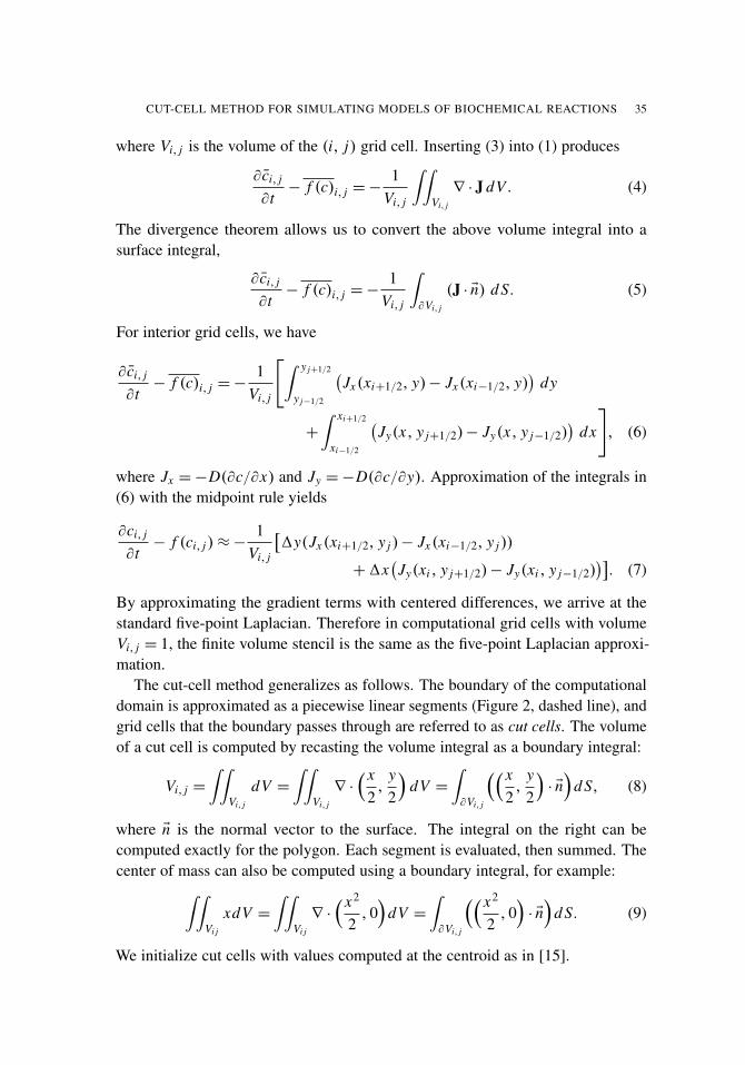
CUT-CELL METHOD FOR SIMULATING MODELS OF BIOCHEMICAL REACTIONS 35
where Vi, j is the volume of the (i, j) grid cell. Inserting (3) into (1) produces
∂ ci, j
∂t− f (c)i, j =−
1Vi, j
∫∫Vi, j
∇ · J dV . (4)
The divergence theorem allows us to convert the above volume integral into asurface integral,
∂ ci, j
∂t− f (c)i, j =−
1Vi, j
∫∂Vi, j
(J · En) d S. (5)
For interior grid cells, we have
∂ ci, j
∂t− f (c)i, j =−
1Vi, j
[∫ y j+1/2
y j−1/2
(Jx(xi+1/2, y)− Jx(xi−1/2, y)
)dy
+
∫ xi+1/2
xi−1/2
(Jy(x, y j+1/2)− Jy(x, y j−1/2)
)dx
], (6)
where Jx =−D(∂c/∂x) and Jy =−D(∂c/∂y). Approximation of the integrals in(6) with the midpoint rule yields
∂ci, j
∂t− f (ci, j )≈−
1Vi, j
[1y(Jx(xi+1/2, y j )− Jx(xi−1/2, y j ))
+1x(Jy(xi , y j+1/2)− Jy(xi , y j−1/2)
)]. (7)
By approximating the gradient terms with centered differences, we arrive at thestandard five-point Laplacian. Therefore in computational grid cells with volumeVi, j = 1, the finite volume stencil is the same as the five-point Laplacian approxi-mation.
The cut-cell method generalizes as follows. The boundary of the computationaldomain is approximated as a piecewise linear segments (Figure 2, dashed line), andgrid cells that the boundary passes through are referred to as cut cells. The volumeof a cut cell is computed by recasting the volume integral as a boundary integral:
Vi, j =
∫∫Vi, j
dV =∫∫
Vi, j
∇ ·
( x2,
y2
)dV =
∫∂Vi, j
(( x2,
y2
)· En)
d S, (8)
where En is the normal vector to the surface. The integral on the right can becomputed exactly for the polygon. Each segment is evaluated, then summed. Thecenter of mass can also be computed using a boundary integral, for example:∫∫
Vi j
xdV =∫∫
Vi j
∇ ·
( x2
2, 0)
dV =∫∂Vi, j
(( x2
2, 0)· En)
d S. (9)
We initialize cut cells with values computed at the centroid as in [15].

36 WANDA STRYCHALSKI, DAVID ADALSTEINSSON AND TIMOTHY ELSTON
Next, we construct the integral on the right side of (5) for a cut cell. In general,there are up to five surface integrals to approximate. Let al,m ∈ [0, 1] represent thefraction of each of the four cell edges covered by the cut cell and a f be the lengthof the line segment representing the boundary. Then (7) becomes
∂ci, j
∂t− f (ci, j )≈−
1Vi, j
[1y
(ai+1/2, j Jx(xci+1/2, y j )− ai−1/2, j Jx(xci−1/2, y j )
)+1x
(ai, j+1/2 Jy(xi , yc j+1/2)− ai, j−1/2 Jy(xi , yc j−1/2)
)+ a f J f
]. (10)
The notation (xci±1/2, y j ) indicates the midpoint of partially covered (xi±1/2, y j )
face. Let
Fi±1/2, j =−ai±1/2, j1y Jx(xci±1/2, y j ), Fi, j±1/2 =−ai, j±1/21x Jy(xi , yc j±1/2).
With this notation, we rewrite the previous equation as
∂ci, j
∂t− f (ci, j )≈
1Vi, j
(Fi+1/2, j − Fi−1/2, j + Fi, j+1/2− Fi, j−1/2− F f
i, j
). (11)
We refer to the Fs as the surface fluxes (Figure 3). On a full edge with al,m = 1 thesurface flux is calculated with centered differences. For example, in Figure 3, wehave
Fi−1/2, j+1 = D1yci, j+1− ci−1, j+1
1x. (12)
The flux gradient across a cut edge, for example (xi−1/2, y j ), is approximated bya linear interpolation of two gradients, which are computed by centered differences.A linear interpolation formula between two points y1 and y2 as a function of a
ci−1, j+1 ci, j+1 ci+1, j+1
ci−1, j ci, j
Fi−1/2, jFi, j+1/2
F fi, j
Outside
Figure 3. Diagram of fluxes for cut cells where shaded boxesindicate cells that are inside the boundary.

CUT-CELL METHOD FOR SIMULATING MODELS OF BIOCHEMICAL REACTIONS 37
parameter µ ∈ [0, 1] isy I= (1−µ)y1+µy2. (13)
In the case of a cut-cell edge, µ= (1+ al,m)/2. For example, to construct Fi−1/2, j
in Figure 3, the gradient at (xi−1/2, y j ) and (xi−1/2, y j+1) is used:
Fi−1/2, j = Dai−1/2, j1y[(1+ ai−1/2, j )
2(ci, j − ci−1, j )
1x
+(1− ai−1/2, j )
2(ci, j+1− ci−1, j+1)
1x
]. (14)
To calculate the flux through a boundary, for example, F fi, j , we compute the
gradient along a line normal to the boundary and centered at the boundary midpoint.To find function values on the normal line, we interpolate using three equally spacedcell-centered points (Figure 4). If the normal line is oriented with an angle ofπ/4 < |θ | < 3π/4 relative to the horizontal grid lines, horizontal grid points areused to compute the values on the line. Otherwise vertical points are used.
The two points computed along the normal line and the value on the boundaryare then used to construct a quadratic polynomial. The concentration gradient iscalculated by differentiating the quadratic polynomial and evaluating the result atthe boundary point c f :
G f=
1d2− d1
[d2
d1(c f− cI
1)−d1
d2(c f− cI
2)
], (15)
cI2
cI1
c f
Outside
Figure 4. White circles indicate interpolated values that dependon the grid-based values.

38 WANDA STRYCHALSKI, DAVID ADALSTEINSSON AND TIMOTHY ELSTON
where cI1 and cI
2 are the interpolated values along the normal line and d1 and d2,respectively, are the distances of these two points from the boundary. The flux F f
i jin (11) is calculated by multiplying G f by the area of the cut-cell edge a f and thediffusion coefficient D. The discretization of the boundary condition (2) becomesthe algebraic equation
DG f+ g(c f )= 0. (16)
Because all gradients are constructed with second-order methods, the overall dis-cretization scheme is second-order in space. Further discussion on the accuracy ofthe spatial discretization scheme can be found in [9].
3.3. Time discretization. Spatial discretizations of (1) and (2) are treated as adifferential-algebraic system of nonlinear equations (DAE). The general form for adifferential-algebraic system is
F(t,C,C ′)= 0, (17)
where C is an (Ng+Nb)×1 vector. The first Ng entries are associated with Cartesiangrid based values in the differential-algebraic system from the discretization of(1) for the chemical species concentrations. These entries have an explicit timederivative term. The Nb remaining entries arise from discretizing the boundaryconditions given in (2) that form algebraic constraints. As noted in [1], reformulatingalgebraic constraints in a nonlinear model as a system of ordinary differentialequations may be time consuming or impossible. DAEs formed by reaction-diffusionequations described in Section 2 are semiexplicit, index-1 systems of the form
C ′1 = F1(C1,C2, t),
0 = F2(C1,C2, t).(18)
C1 represents the first Ng variables and C2 represents the remaining Nb variables.Equation (18) is an index-1 system if and only if ∂F2/∂C2 is nonsingular [1].Ordinary differential equations are index-0.
We use the DASPK solver described in [2] as a time integrator for our differentialalgebraic system. In DAPSK, backward differentiation formulas (BDF) discretizethe time derivative in (17). A basic implicit method with a backward Euler timediscretization of (17) is given by,
F(
tn+1,Cn+1,Cn+1
−Cn
1t
)= 0, (19)
where n is defined such that tn= n1t . Newton’s method can be used to solve the
resulting nonlinear equations for Cn+1,
Cn+1m+1 = Cn+1
m −
(∂F∂C+
11t
∂F∂C ′
)∣∣∣−1
Cn+1m
F(
tn+1,Cn+1m ,
Cn+1m −Cn
1t
), (20)

CUT-CELL METHOD FOR SIMULATING MODELS OF BIOCHEMICAL REACTIONS 39
where m is the index of the Newton iteration. In order to achieve higher-ordertemporal accuracy, a higher-order interpolating polynomial is used to approximatethe time derivative.
In a k-step BDF, the time derivative is replaced by the derivative of an inter-polating polynomial at k + 1 times tn+1, tn . . . , tn+1−k evaluated at tn+1. If weapproximate the derivative using a kth order stencil using k known values and theimplicit value Cn+1 we get
C ′ n+1≈
11t
(α0Cn+1
+
k∑i=1
αi Cn+1−i). (21)
The coefficients of the BDF are given by αi s. In DAPSK, these values are coefficientsof the Newton divided difference interpolating polynomial [1]. The default order ofthe BDF method in DASPK is five.
The new implicit equation to be solved at each time step is
F(
tn+1,Cn+1,11t
(α0Cn+1
+
k∑i=1
αi Cn+1−i))= 0. (22)
This can be rewritten as
F(
tn+1,Cn+1,α0
1tCn+1
+ v)= 0, (23)
where v is a vector that depends on previously computed time values. Details ofchoosing step-size, starting selection and variable order strategies are found in [1].The nonlinear system is solved with a modified Newton’s method, given by
Cn+1m+1 = Cn
m − ζ(∂F∂C+α0
1t∂F∂C ′
)∣∣∣−1
Cn+1m
F(
tn+1,Cn+1m ,
α0
1tCn+1
m + v), (24)
where ζ is a constant chosen to speed up convergence and m is the iteration index.Each step of the Newton iteration requires inverting the matrix
A =∂F∂C+α0
1t∂F∂C ′
. (25)
We store this matrix in sparse triple format, and use routines from SPARSKIT [20]to solve the linear system iteratively. The generalized minimal residual (GMRES)method [21] with an incomplete LU (ILU) preconditioner is used to solve the linearsystem.
4. Results
4.1. Convergence tests. To demonstrate the accuracy of our method on a domaincontaining all types of cut cells, the convergence of our method is compared against

40 WANDA STRYCHALSKI, DAVID ADALSTEINSSON AND TIMOTHY ELSTON
an exact solution on a circle. The exact solution to the diffusion equation with azero Dirichlet boundary condition can be found in terms of Bessel functions. Let λdenote the first root of the Bessel function J0(x), and r be the radius of the circlecentered at the point (0.5, 0.5). Then the expression
f (x, y, t)= exp(−D
(λr
)2t)
J0
(λ
√
(x − 0.5)2+ (y− 0.5)2
r
)(26)
is an exact solution to the diffusion equation.For this example, the error is computed as the difference between computed
solution values on a triangular grid subtracted from the exact solution. The grids forboth two dimensional triangular meshes were the same. For purposes of generatingthe following convergence data, the spatial steps 1x and 1y are equal and set to1/N , where N is the grid size. The time step 1t is set to 1x/4 (that is, it is refinedwith the spatial step size). Because DASPK uses variable time steps, the output atthe time step requested might be interpolated as described in [1]. A time series ofthe truncation error in the infinity norm over time is shown in Figure 5. Table 1lists the truncation error at the simulation time t = 0.4. The convergence rate r iscalculated as
r = loge1
e2
/log
1x1
1x2, (27)
where e1 and e2 are errors computed in norms with grid spacing 1x1 and 1x2. Alog-log plot of truncation error as a function of the spatial step is shown in Figure 6.The error was calculated with the computed and exact solutions at the time value oft = 0.4. The results of this analysis demonstrate global second-order accuracy ofthe numerical method.
Next we tested a nonlinear system in which a protein C can exist in two dis-tinct chemical states: active and inactive. The reactions that convert the proteinbetween the two states are assumed to follow Michaelis–Menten kinetics, whichdescribes the kinetics of many enzymatic reactions including phosphorylation anddephosphorylation events [11]. The protein C is deactivated in the interior of the
Grid size Time step L2 norm r L1 norm r L∞ norm r
50 × 50 5.00·10−3 2.95·10−4− 2.61·10−4
− 5.46·10−4−
100 × 100 2.50·10−3 4.94·10−5 2.58 4.32·10−5 2.59 9.28·10−5 2.56200 × 200 1.25·10−3 1.05·10−5 2.24 9.20·10−6 2.23 2.09·10−5 2.15400 × 400 6.25·10−4 2.42·10−6 2.11 2.13·10−6 2.11 5.42·10−6 1.95
Table 1. The norms and convergence rates for the diffusion equa-tion at the time value of 0.4.

CUT-CELL METHOD FOR SIMULATING MODELS OF BIOCHEMICAL REACTIONS 41
1.75 ×10⁻⁴
3.97 ×10⁻⁵
1.03 ×10⁻⁵
L ∞
Nor
m o
f Tru
ncat
ion
Erro
r
10-5
0
5
10
15
20
25
30
Time0 0.05 0.10 0.15 0.20 0.25 0.30 0.35 0.40
Figure 5. L∞-norm truncation error for the diffusion equation,with size N = 100, 200, 400 (from top to bottom). The time step ateach refinement was set to 1/(4N ).
computational domain according to the following equations:
∂Ci
∂t= D1Ci +
k2Ca
Km2+Ca,
∂Ca
∂t= D1Ca −
k2Ca
km2+Ca, (28)
where Ci and Ca are the concentrations of inactive and active protein, respectively,k2 is the maximum deactivation rate, and Km2 is the Michaelis constant. Activation
Second order referenceL∞ normL1 normL2 normFirst order reference
Trun
catio
n Er
ror
10-5
0.1
1
10
100
Grid size50 100 200 400
Figure 6. Truncation error for the diffusion equation at the timevalue of 0.4. The convergence data is the same as in Table 1.

42 WANDA STRYCHALSKI, DAVID ADALSTEINSSON AND TIMOTHY ELSTON
occurs on the boundary, ∂�, according to the following boundary conditions:
−DEn · ∇Ci |∂� =k1SCi
Km1+Ci
∣∣∣∂�, −DEn · ∇Ca|∂� =−
k1SCi
Km1+Ci
∣∣∣∂�, (29)
where k1 is the maximum activation rate and Km1 is the Michaelis constant. Theequations are solved in the domain
�(r, θ)= r ≤ 0.3− 0.09 sin(4θ). (30)
In our simulation, � is shifted to the center of the unit box. The initial concentrationof inactive protein is assumed to be constant and equal to 1. There is initially noactive protein. Figure 7 shows a plot of the active concentration at t = 0.25.For visualization purposes, the computational domain and boundary points aretriangulated with Triangle [27]. The concentration of the active protein is shown asa cross-section of the two-dimensional geometry at several time values in Figure7, bottom. The constants (see figure caption) were arbitrarily chosen to generate agradient. Execution times for Mac Pro desktop computer with dual-core 2.66 GHzIntel Xeon processors for different grid sizes are listed in Table 2.
We compute the error as the difference between successive grid refinements asfollows. The truncation error function E(x, y, t) is defined on interior values of thecoarser grid. Computed solution values located in coarse grid cut cells are excludedfrom the domain. This includes some values located in interior points for the morerefined grid (Figure 8). The truncation error function is defined as
E(x, y, t)= c1x(x, y, t)− c1x/2(x, y, t). (31)
The coarse grid values are located in the center of a box defined by four refined gridvalues. Four refined grid values are averaged and subtracted from one coarse value.Because the time integration is handled implicitly, a different convergence rate ofthe truncation error in cut cells and boundary values would affect the convergence
ExecutionGrid size Time step time
50 × 50 5.000·10−3 1.76 s100 × 100 2.500·10−3 5.81 s200 × 200 1.250·10−3 32.15 s400 × 400 6.250·10−4 203.95 s800 × 800 3.125·10−4 1202.18 s
Table 2. Execution times for the two-species model. The end timeof the simulation was t = 0.5.
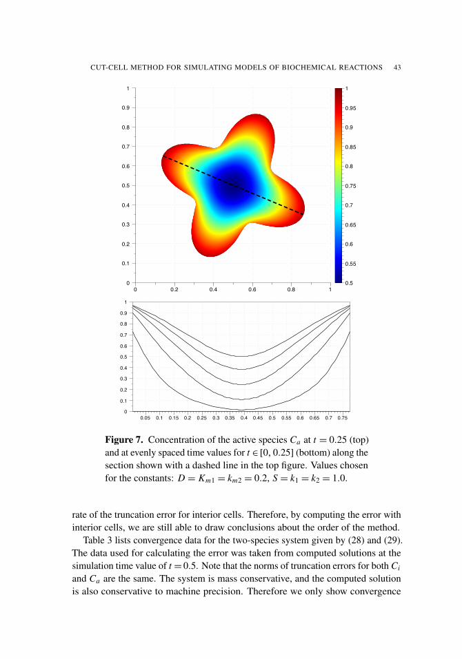
CUT-CELL METHOD FOR SIMULATING MODELS OF BIOCHEMICAL REACTIONS 43
0 0.2 0.4 0.6 0.8 10
0.1
0.2
0.3
0.4
0.5
0.6
0.7
0.8
0.9
1
0.5
0.55
0.6
0.65
0.7
0.75
0.8
0.85
0.9
0.95
1
0.05 0.1 0.15 0.2 0.25 0.3 0.35 0.4 0.45 0.5 0.55 0.6 0.65 0.7 0.750
0.1
0.2
0.3
0.4
0.5
0.6
0.7
0.8
0.9
1
Figure 7. Concentration of the active species Ca at t = 0.25 (top)and at evenly spaced time values for t ∈ [0, 0.25] (bottom) along thesection shown with a dashed line in the top figure. Values chosenfor the constants: D = Km1 = km2 = 0.2, S = k1 = k2 = 1.0.
rate of the truncation error for interior cells. Therefore, by computing the error withinterior cells, we are still able to draw conclusions about the order of the method.
Table 3 lists convergence data for the two-species system given by (28) and (29).The data used for calculating the error was taken from computed solutions at thesimulation time value of t = 0.5. Note that the norms of truncation errors for both Ci
and Ca are the same. The system is mass conservative, and the computed solutionis also conservative to machine precision. Therefore we only show convergence
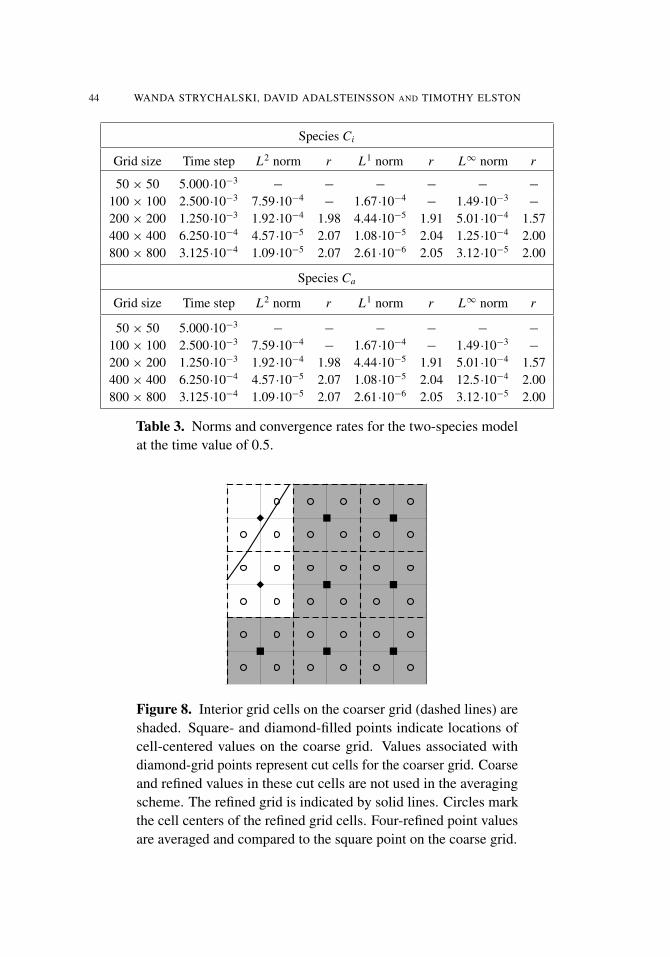
44 WANDA STRYCHALSKI, DAVID ADALSTEINSSON AND TIMOTHY ELSTON
Species Ci
Grid size Time step L2 norm r L1 norm r L∞ norm r
50 × 50 5.000·10−3− − − − − −
100 × 100 2.500·10−3 7.59·10−4− 1.67·10−4
− 1.49·10−3−
200 × 200 1.250·10−3 1.92·10−4 1.98 4.44·10−5 1.91 5.01·10−4 1.57400 × 400 6.250·10−4 4.57·10−5 2.07 1.08·10−5 2.04 1.25·10−4 2.00800 × 800 3.125·10−4 1.09·10−5 2.07 2.61·10−6 2.05 3.12·10−5 2.00
Species Ca
Grid size Time step L2 norm r L1 norm r L∞ norm r
50 × 50 5.000·10−3− − − − − −
100 × 100 2.500·10−3 7.59·10−4− 1.67·10−4
− 1.49·10−3−
200 × 200 1.250·10−3 1.92·10−4 1.98 4.44·10−5 1.91 5.01·10−4 1.57400 × 400 6.250·10−4 4.57·10−5 2.07 1.08·10−5 2.04 12.5·10−4 2.00800 × 800 3.125·10−4 1.09·10−5 2.07 2.61·10−6 2.05 3.12·10−5 2.00
Table 3. Norms and convergence rates for the two-species modelat the time value of 0.5.
Figure 8. Interior grid cells on the coarser grid (dashed lines) areshaded. Square- and diamond-filled points indicate locations ofcell-centered values on the coarse grid. Values associated withdiamond-grid points represent cut cells for the coarser grid. Coarseand refined values in these cut cells are not used in the averagingscheme. The refined grid is indicated by solid lines. Circles markthe cell centers of the refined grid cells. Four-refined point valuesare averaged and compared to the square point on the coarse grid.
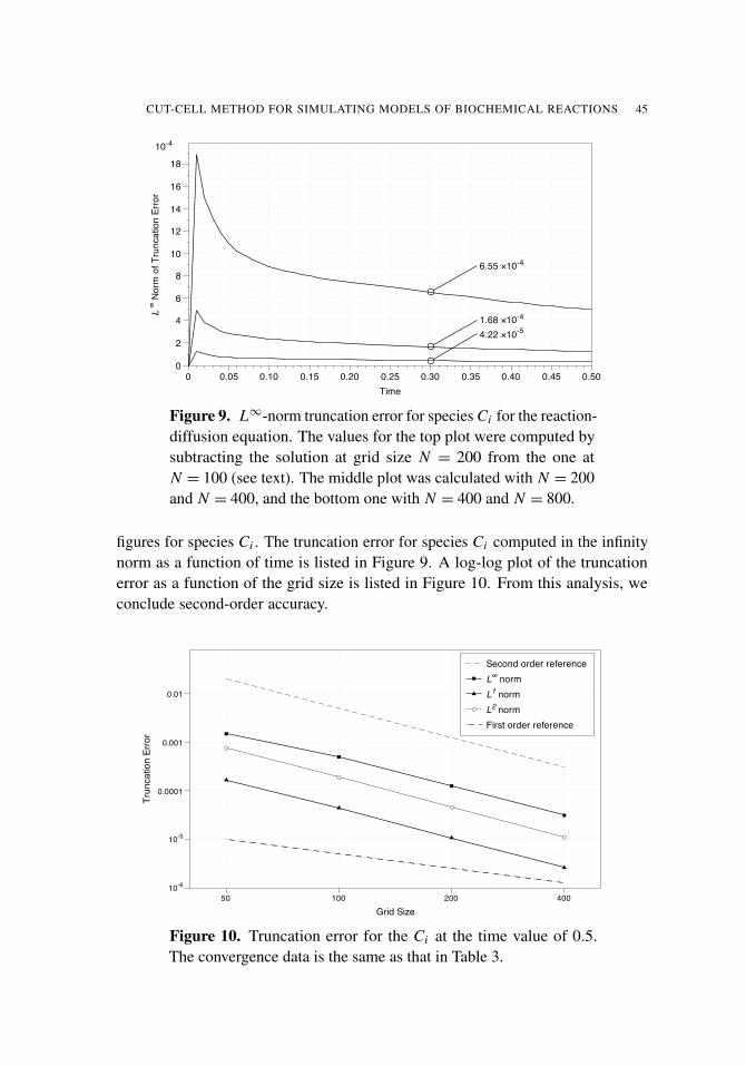
CUT-CELL METHOD FOR SIMULATING MODELS OF BIOCHEMICAL REACTIONS 45
6.55 ×10⁻⁴
1.68 ×10⁻⁴
4.22 ×10⁻⁵
L ∞
Nor
m o
f Tru
ncat
ion
Erro
r10-4
0
2
4
6
8
10
12
14
16
18
Time0 0.05 0.10 0.15 0.20 0.25 0.30 0.35 0.40 0.45 0.50
Figure 9. L∞-norm truncation error for species Ci for the reaction-diffusion equation. The values for the top plot were computed bysubtracting the solution at grid size N = 200 from the one atN = 100 (see text). The middle plot was calculated with N = 200and N = 400, and the bottom one with N = 400 and N = 800.
figures for species Ci . The truncation error for species Ci computed in the infinitynorm as a function of time is listed in Figure 9. A log-log plot of the truncationerror as a function of the grid size is listed in Figure 10. From this analysis, weconclude second-order accuracy.
Second order referenceL∞ normL1 normL2 normFirst order reference
Trun
catio
n Er
ror
10-6
10-5
0.0001
0.001
0.01
Grid Size50 100 200 400
Figure 10. Truncation error for the Ci at the time value of 0.5.The convergence data is the same as that in Table 3.

46 WANDA STRYCHALSKI, DAVID ADALSTEINSSON AND TIMOTHY ELSTON
4.2. A two-compartment model. In this model, we have two compartments: cyto-plasm and nucleus. The cellular geometry was taken from a yeast cell undergoingchemotrophic growth in the direction of a pheromone gradient [8]. Proteins involvedin the pheromone response pathway are known to localize on the plasma membrane,the nucleus, and in the cytosol [7]. The nucleus is modeled as a circle locatedtoward the front of the cell. Because yeast cells are three dimensional, we modelthe top view of the cell as in [6], where membrane-bound species are located inthe interior of the computational domain but are assumed to diffuse slower thancytosolic forms.
The model consists of two species, A and C , with inactive and active forms.Protein C is allowed to enter and exit the nucleus, whereas protein A is restrictedto the cytoplasm (Figure 11, top).
A! A!
CA!! C!
C! ! C
0.2 0.4 0.6 0.8 1
0
0.1
0.2
0.3
0.4
0.5
0.6
0.7
0.8
0.9
1
0.75
0.76
0.77
0.78
0.79
0.8
0.81
0.82
0.83
0.84
0.85
0.86
0.87
Figure 11. Two-compartment model. Top: reactions and speciesin the two-compartment model. Bottom: steady-state concentrationvalues for active C species in the cytoplasm and nucleus.

CUT-CELL METHOD FOR SIMULATING MODELS OF BIOCHEMICAL REACTIONS 47
Initially both A and C are in their inactive forms. At the beginning of thesimulation, the reaction rate for the activation of A, k0, is instantaneously increasedfrom 0 to 1. This is meant to model the cell receiving an external signal. Once A isactivated it is assumed to interact with the cell membrane, causing a reduction in theprotein’s diffusion coefficient [30]. The active form of A can then activate proteinC . The active form of C is only deactivated within the nucleus. This simple modelcaptures some of the signaling events that occur during the pheromone response ofyeast [28]. If we denote the concentration of a chemical species with brackets, theequations for the cytoplasmic species are:
∂[Ac]
∂t= D11[Ac] − k0[Ac],
∂[A∗c ]∂t= D21[A∗c ] + k0[Ac],
∂[Cc]
∂t= D11[Cc] − k1[A∗c ][Cc],
∂[C∗c ]∂t= D11[C∗c ] + k1[A∗c ][Cc],
(32)
where the asterisks denote the active form of the protein, D1 is the diffusioncoefficient in the cytoplasm, D2 is diffusion coefficient in the membrane, and the ksrepresent the reaction rates. Subscripts indicate cytosolic and nuclear species. Theboundary conditions at the cell membrane ∂�1 are no flux for all chemical species.The nuclear boundary conditions for A species are also no flux, whereas C speciesare allowed to move through the nuclear membrane ∂�2 and satisfy the conditions
−D1(En · ∇[Cc])|∂�2 =−k2([Cn] − [Cc])|∂�2,
−D1(En · ∇[C∗c ])|∂�2 =−k2([C∗n ] − [C∗
c ])|∂�2,
−D1(En · ∇[Cn])|∂�2 = k2([Cn] − [Cc])|∂�2,
−D1(En · ∇[C∗n ])|∂�2 = k2([C∗n ] − [C∗
c ])|∂�2 .
(33)
Nuclear C∗ is deactivated according to the equations
∂[Cn]
∂t= D11[Cn] + k3[C∗n ],
∂[C∗n ]∂t= D11[C∗n ] − k3[C∗n ]. (34)
The steady-state spatial distribution of active C is illustrated in Figure 11, bottom.All reaction constants were arbitrarily chosen to be 1, D1=0.1, D2=0.01, and1x=1/200. The initial values were zero except for [Ac](x, y, 0) = [Cc](x, y, 0) = 1.The execution time of the simulation to run from t = 0 until t = 20 was 150 secondson Mac Pro desktop computer with dual-core 2.66 GHz Intel Xeon processors.
To verify that the system is close a steady-state solution at t = 20, we subtractedthe solution of active C in the cytoplasm [C∗c ] for all times from the assumed steady-state solution at the time value of t = 20. If the system exponentially converges tothe computed solution at t = 20, we assume this time value is close to steady-state.Figure 12 shows the infinity norm of the difference between the computed solution

48 WANDA STRYCHALSKI, DAVID ADALSTEINSSON AND TIMOTHY ELSTON
Difference from Steady StateExponential Fit
L∞ N
orm
of D
iffer
ence
10-10
10-9
10-8
10-7
10-6
10-5
0.0001
0.001
0.01
0.1
1
10
Time0 2 4 6 8 10 12 14 16 18 20
Figure 12. Solid line: norm of difference of the computed solutionat the assumed steady-state value at t = 20 from computed solutionover time. Dashed line: exponential fit.
and the solution at t = 20 sampled over time. Based on this data, the system isclose to its steady-state solution.
The model simulation suggests a spatial activation gradient can be generated bythe position of the nucleus. The inactivation of C in the nucleus leads to a higherconcentration of active protein in the rear of the cell in spite of a uniform spatialsignal from active A.
4.3. Rho family GTPase model. The Rho family of GTPases regulates many cel-lular functions, including polarization and motility. We created a model with threekey members of this family, Cdc42, Rac, and Rho; the interactions, based on [3],can be schematically represented as follows:
Signal Cdc42 Rac Rho
A more complicated model involving these proteins in one dimension can be foundin [6]. As in the previous example, we assume a top view of a three dimensionalcell with membrane bound active forms and cytosolic inactive forms of the threeproteins. The model has a total of six species. The cell boundary ∂� is taken fromsupplemental material from [19].

CUT-CELL METHOD FOR SIMULATING MODELS OF BIOCHEMICAL REACTIONS 49
In our model, a uniform extracellular signal triggers the activation of Cdc42protein on the cell edge,
−DEn · ∇ [Cdc42i ]∣∣∂�=
k1S [Cdc42i ]Km1+ [Cdc42i ]
∣∣∣∂�,
−DEn · ∇ [Cdc42a]∣∣∂�=−
k1S [Cdc42i ]km2+ [Cdc42i ]
∣∣∣∂�.
(35)
In the cell interior, active Cdc42 is inactivated. A positive feedback loop increasesthe activation of Cdc42,
∂ [Cdc42i ]∂t
= D1 [Cdc42i ]+k2 [Cdc42a]
Km3+ [Cdc42a]−
k3 [Cdc42a] [Cdc42i ]Km4+ [Cdc42i ]
,
∂ [Cdc42a]∂t
= D1 [Cdc42a]−k2 [Cdc42a]
km5+ [Cdc42a]+
k3 [Cdc42a] [Cdc42i ]km6+ [Cdc42i ]
.
(36)
Rac is activated by Cdc42, and a positive feedback loop increases the concentrationof active Rac. Active Rho increases the deactivation of Rac in the cytosol,
∂[Raci ]
∂t= D1[Raci ]+
(k4[Rhoa]+k5)[Raca]
Km7+[Raca]−(k6[Cdc42a]+k7[Raca])[Raci ]
Km8+[Raci ],
∂[Raca]
∂t= D1[Raca]−
(k4[Rhoa]+k5)[Raca]
km9+[Raca]+(k6[Cdc42a]+k7[Raca])[Raci ]
km10+[Raci ].
Rho is activated by the active form of Rac and deactivated in the interior,
∂ [Rhoi ]∂t
= D1 [Rhoi ] +k8 [Rhoa]
Km11+ [Rhoa]−
k9 [Raca] [Rhoi ]Km12+ [Rhoi ]
,
∂ [Rhoa]∂t
= D1 [Rhoa]−k8 [Rhoa]
km13+ [Rhoa]+
k9 [Raca] [Rhoi ]km14+ [Rhoi ]
.
(37)
The boundary conditions for Rac and Rho species are no flux. The steady-statedistribution is displayed in Figure 13. To achieve these results, a step size 1x =1/200 and a diffusion coefficient D = 0.1 were used. The reaction constantsfor the simulation were arbitrarily chosen as follows: S = k3 = k5 = k7 = 1.0,k2 = k4 = k8 = 3.0, k1 = k6 = k9 = 5.0, and all Kmi and kmi equal to 0.2.
The initial concentration of inactive chemical species was set to one and zero foractive species. The execution time was 217 seconds for 1600 time steps on a MacPro desktop computer with dual-core 2.66 GHz Intel Xeon processors.
In this model, a gradient is formed by protein activation on the cell edge, andpropagated to the downstream signaling components Rac and Rho. Figure 13 showsthat filopodia and thin protrusions have higher activation levels due the increasedratio of cell membrane to cell volume in these regions [16].

50 WANDA STRYCHALSKI, DAVID ADALSTEINSSON AND TIMOTHY ELSTON
Inactive Active
0 0.2 0.4 0.6 0.8 10
0.1
0.2
0.3
0.4
0.5
0.6
0.7
0.8
0.9
1
0
0.05
0.1
0.15
0.2
0.25
0.3
0.35Cdc42i
0 0.2 0.4 0.6 0.8 10
0.1
0.2
0.3
0.4
0.5
0.6
0.7
0.8
0.9
1
0.65
0.7
0.75
0.8
0.85
0.9
0.95
1Cdc42a
0 0.2 0.4 0.6 0.8 10
0.1
0.2
0.3
0.4
0.5
0.6
0.7
0.8
0.9
1 Raci
0.17
0.18
0.19
0.2
0.21
0.22
0.23
0.24
0 0.2 0.4 0.6 0.8 10
0.1
0.2
0.3
0.4
0.5
0.6
0.7
0.8
0.9
1 Raca
0.76
0.77
0.78
0.79
0.8
0.81
0.82
0.83
0 0.2 0.4 0.6 0.8 10
0.1
0.2
0.3
0.4
0.5
0.6
0.7
0.8
0.9
1 Rhoi
0.27
0.275
0.28
0.285
0.29
0.295
0.3
0 0.2 0.4 0.6 0.8 10
0.1
0.2
0.3
0.4
0.5
0.6
0.7
0.8
0.9
1 Rhoa
0.7
0.705
0.71
0.715
0.72
0.725
0.73
Figure 13. Rho GTPase model: steady-state distribution of proteinconcentration amounts in a fibroblast. The boundary was takenfrom a live cell image [19]. Values chosen for the constants: S =k3 = k5 = k7 = 1.0, k2 = k4 = k8 = 3.0, k1 = k6 = k9 = 5.0, andall Kmi and kmi equal to 0.2.
5. Conclusions
We have developed an accurate and efficient cut-cell method for simulating spatialmodels of signaling pathways in realistic cellular geometries. We demonstratedour method using models that consist of multiple species interacting in multiple

CUT-CELL METHOD FOR SIMULATING MODELS OF BIOCHEMICAL REACTIONS 51
compartments. The examples were chosen to illustrate the numerical methodsand therefore lack many details found in real biological signaling systems. Inparticular, feedback and feed forward control mechanisms that regulate pathwayactivity were not considered in detail. Our numerical methods provide importanttools for investigating such regulatory mechanisms in realistic cell geometriesand, therefore, should provide important insights into the ways signaling networksprocess and transmit information.
Our algorithm extends previous work on embedded boundary methods [5; 9;15; 25]. These methods have been implemented in two and three dimension forPoisson’s equation, the heat equation, and hyperbolic conservation laws. Ourformulation extends these methods to systems of reaction-diffusion equations withnonlinear reactions in the interior as well as nonlinear reactions affecting boundaryvalues. The boundary conditions treated in previous work [9; 15; 25] have beenhomogeneous Dirichlet and Neumann, which is not sufficient for many modelsof signaling pathways [16]. In [15], a second-order implicit method was used toupdate the heat equation in time [29]. In our method, we use an implicit nonlinearsolver to handle nonlinear reactions occurring in the interior. An advantage of thedifferential-algebraic formulation is the ability to treat the boundary conditionsas algebraic constraints. This allows us to handle reactions that take place on thephysical boundary of the reaction-diffusion equation.
One limitation of the finite volume discretization arises from the interpolationmethod to obtain the normal derivative to the surface as shown in Figure 4. Cut cellsmust not have a zero volume cell within two rows or columns. For biological cellswith long, thin or irregularly-shaped components such as neurons, mesh adaptiverefinement may be needed to resolve the cellular geometry.
The underlying Cartesian-grid based finite volume discretization allows us touse advection schemes originally developed for hyperbolic conservation laws tosimulate active transport or motility. In future reports, we will show how level setmethods [18; 26] can be combined with biochemical reaction networks to investigatethe effect of moving boundaries on cell signaling. Future work also includes a three-dimensional implementation of our fixed boundary algorithm. A three-dimensionalextension of our method could be coupled with the method for simulating diffusionon a surface presented in [24] to obtain an algorithm for simulating models that takeinto account processes that occur both in the cytoplasm and on the cell membrane.
6. Acknowledgments
We thank Meng Jin and Yi Wu for insightful discussions. This work was supportedby NIH grants R01-GM079271 and R01-GM078994.

52 WANDA STRYCHALSKI, DAVID ADALSTEINSSON AND TIMOTHY ELSTON
References
[1] K. E. Brenan, S. L. Campbell, and L. R. Petzold, Numerical solution of initial-value problems indifferential-algebraic equations, Classics in Applied Mathematics, no. 14, SIAM, Philadelphia,1996. MR 96h:65083 Zbl 0844.65058
[2] P. N. Brown, A. C. Hindmarsh, and L. R. Petzold, Using Krylov methods in the solution oflarge-scale differential-algebraic systems, SIAM J. Sci. Comput. 15 (1994), no. 6, 1467–1488.MR 95g:65092 Zbl 0812.65060
[3] K. Burridge and K. Wennerberg, Rac and Rho take center stage, Cell 116 (2004), 167–179.[4] P. Colella, D. Graves, T. Ligocki, D. Trebotich, and B. V. Straalen, Embedded boundary
algorithms and software for partial differential equations, J. Phys. Conf. Ser. 125 (2008),012084.
[5] P. Colella, D. T. Graves, B. J. Keen, and D. Modiano, A Cartesian grid embedded boundarymethod for hyperbolic conservation laws, J. Comput. Phys. 211 (2006), no. 1, 347–366. MR2006i:65142 Zbl 1120.65324
[6] A. T. Dawes and L. Edelstein-Keshet, Phosphoinositides and Rho proteins spatially regulateactin polymerization to initiate and maintain directed movement in a one-dimensional model ofa motile cell, Biophys. J. 92 (2007), no. 3, 744–768.
[7] H. G. Dohlman, G Proteins and pheromone signaling, Annu. Rev. Physiol. 64 (2002), 129–152.[8] N. Hao, S. Nayak, M. Behar, R. H. Shanks, M. J. Nagiec, B. Errede, J. Hasty, and T. C. Elston,
Regulation of cell signaling dynamics by the protein kinase-scaffold ste5, Mol. Cell. 30 (2008),no. 5, 649–656.
[9] H. Johansen and P. Colella, A Cartesian grid embedded boundary method for Poisson’s equationon irregular domains, J. Comput. Phys. 147 (1998), no. 1, 60–85. MR 99m:65231 Zbl0923.65079
[10] B. N. Kholodenko, Cell-signalling dynamics in time and space, Nat. Rev. Mol. Cell. Biol. 7(2006), no. 3, 165–176.
[11] B. N. Kholodenko, G. C. Brown, and J. B. Hoek, Diffusion control of protein phosphorylation insignal transduction pathways, Biochem. J. 350 (2000), no. Pt. 3, 901–907.
[12] H. Levine, D. A. Kessler, and W. J. Rappel, Directional sensing in eukaryotic chemotaxis: Abalanced inactivation model, Proc. Natl. Acad. Sci. USA. 103 (2006), no. 26, 9761–9766.
[13] T. J. Ligocki, P. O. Schwartz, J. Percelay, and P. Colella, Embedded boundary grid generationusing the divergence theorem, implicit functions, and constructive solid geometry, J. Phys. Conf.Ser. 125 (2008), 012080 (5pp).
[14] R. Malladi, J. A. Sethian, and B. C. Vemuri, A fast level set based algorithm for topology-independent shape modeling, J. Math. Imaging Vision 6 (1996), 269–289. MR 97a:68174
[15] P. McCorquodale, P. Colella, and H. Johansen, A Cartesian grid embedded boundary methodfor the heat equation on irregular domains, J. Comput. Phys. 173 (2001), no. 2, 620–635.MR 2002h:80009 Zbl 0991.65099
[16] J. Meyers, J. Craig, and D. J. Odde, Potential for control of signaling pathways via cell size andshape, Curr. Biol. 16 (2006), no. 17, 1685–1693.
[17] S. R. Neves, P. Tsokas, A. Sarkar, E. A. Grace, P. Rangamani, S. M. Taubenfeld, C. M. Alberini,J. C. Schaff, R. D. Slizter, I. I. Moraru, and R. Iyengar, Cell shape and negative links in regulatorymotifs together control spatial information flow in signaling networks, Cell 133 (2008), no. 4,666–680.
[18] S. Osher and J. A. Sethian, Fronts propagating with curvature-dependent speed: algorithmsbased on Hamilton–Jacobi formulations, J. Comput. Phys. 79 (1988), no. 1, 12–49. MR89h:80012 Zbl 0659.65132

CUT-CELL METHOD FOR SIMULATING MODELS OF BIOCHEMICAL REACTIONS 53
[19] O. Pertz, L. Hodgson, R. Klemke, and K. Hahn, Spatiotemporal dynamics of RhoA activity inmigrating cells, Nature 440 (2006), no. 7087, 1069–1072.
[20] Y. Saad, SPARSKIT: A basic tool-kit for sparse matrix computations (version 2), 2005, usermanual.
[21] Y. Saad and M. H. Schultz, GMRES: a generalized minimal residual algorithm for solvingnonsymmetric linear systems, SIAM J. Sci. Statist. Comput. 7 (1986), 856–869. MR 87g:65064Zbl 0599.65018
[22] J. C. Schaff, B. M. Slepchenko, Y. Choi, J. Wagner, D. Resasco, and L. Loew, Analysis ofnonlinear dynamics on arbitrary geometries with the Virtual Cell, Chaos 11 (2001), no. 1,115–131. Zbl 0992.92021
[23] I. C. Schneider, E. M. Parrish, and J. M. Haugh, Spatial analysis of 3’ phosphoinositide signalingin living fibroblasts, III: influence of cell morphology and morphological polarity, Biophys. J.89 (2005), no. 2, 1420–1430.
[24] P. Schwartz, D. Adalsteinsson, P. Colella, A. Arkin, and M. Onsum, Numerical computation ofdiffusion on a surface, P. Natl. Acad. Sci. USA 102 (2005), no. 32, 11151–11156.
[25] P. Schwartz, M. Barad, P. Colella, and T. Ligocki, A Cartesian grid embedded boundary methodfor the heat equation and Poisson’s equation in three dimensions, J. Comput. Phys. 211 (2006),no. 2, 531–550. MR 2006e:65194 Zbl 1086.65532
[26] J. A. Sethian, Level set methods and fast marching methods: evolving interfaces in computationalgeometry, fluid mechanics, computer vision, and materials science, 2nd ed., Cambridge Univ.Press, Cambridge, 1999. MR 2000c:65015 Zbl 0973.76003
[27] J. R. Shewchuk, Engineering a 2D quality mesh generator and Delaunay triangulator, Appliedcomputational geometry (M. C. Lin and D. Manocha, eds.), Lecture Notes in Computer Science,no. 1148, Springer, Berlin, 1996, pp. 203–222. MR 97k:68004
[28] Y. Shimada, M. P. Gulli, and M. Peter, Nuclear sequestration of the exchange factor Cdc24 byFar1 regulates cell polarity during yeast mating, Nat. Cell. Biol. 2 (2000), no. 2, 117–124.
[29] E. H. Twizell, A. B. Gumel, and M. A. Arigu, Second-order, L0-stable methods for the heatequation with time-dependent boundary conditions, Adv. Comput. Math. 6 (1996), no. 3-4,333–352 (1997). MR 97m:65164 Zbl 0872.65084
[30] J. Valdez-Taubas and H. R. B. Pelham, Slow diffusion of proteins in the yeast plasma membraneallows polarity to be maintained by endocytic cycling, Curr. Biol. 13 (2003), no. 18, 1636–1640.
[31] O. C. Zienkiewicz and R. L. Taylor, The finite element method set, 6th ed., Butterworth–Heinemann, 2005.
Received June 24, 2009. Revised December 4, 2009.
WANDA STRYCHALSKI: [email protected] Center for Interdisciplinary Applied Mathematics, Department of Mathematics,University of North Carolina at Chapel Hill, Chapel Hill, NC 27599, United Stateshttp://www.unc.edu/~wandastr
DAVID ADALSTEINSSON: [email protected] Center for Interdisciplinary Applied Mathematics, Department of Mathematics,University of North Carolina at Chapel Hill, Chapel Hill, NC 27599, United Stateshttp://amath.unc.edu/David/David
TIMOTHY ELSTON: [email protected] of Pharmacology, University of North Carolina at Chapel Hill, Chapel Hill, NC 27599,United Stateshttp://www.amath.unc.edu/Faculty/telston/


COMM. APP. MATH. AND COMP. SCI.Vol. 5, No. 1, 2010
AN URN MODEL ASSOCIATED WITH JACOBI POLYNOMIALS
F. ALBERTO GRÜNBAUM
We consider an urn model leading to a random walk that can be solved explicitlyin terms of the well-known Jacobi polynomials.
1. Urn models and orthogonal polynomials
There are two simple and classical models in statistical mechanics which haverecently been associated with very important classes of orthogonal polynomials.The oldest one of these models is due to D. Bernoulli (1770) and S. Laplace (1810),while the more recent model is due to Paul and Tatiana Ehrenfest (1907) [6]. Whileboth of these models are featured in very classical texts in probability theory, suchas [7], the connection with orthogonal polynomials is of much more recent vintage.In fact, the polynomials in question due to Krawtchouk and Hahn had not beenrecognized as basic objects with rich properties until around 1950. For a fewpertinent and useful references, see [1; 2; 4; 5; 11; 14; 16; 18].
From these comments one could get the impression that the relations betweenorthogonal polynomials — especially some well-known classes of them — are onlya matter of historical interest. Nothing could be further from the truth: thereare several areas of probability and mathematical physics where recent importantprogress hinges on the connections with orthogonal polynomials.
The entire area of random matrix theory starts with the work of E. Wigner and F.Dyson and reaches a new stage in the hands of M. Mehta who brought the powerof orthogonal polynomials into the picture.
In the area of random growth processes, the seminal work of K. Johanssondepends heavily on orthogonal polynomials, specifically Laguerre and Meixnerones; see [15].
The connection between birth-and-death processes and orthogonal polynomialshas many parents, but the people that made the most of it are S. Karlin and J.McGregor [17]. We will have a chance to go back to their work in connectionwith our model here. The ideas of using the spectral analysis of the corresponding
MSC2000: primary 33C45, 60J10; secondary 60G99.Keywords: random walks, urn models, Jacobi polynomials, orthogonal polynomials.The author was supported in part by NSF Grant DMS-0603901 and AFOSR Contract FA9550-08-1-0169.
55

56 F. ALBERTO GRÜNBAUM
one-step transition matrix have been pushed recently in the case of quantum randomwalks, an area where physics, computer science and mathematics could makeimportant contributions. See [3; 12].
The study of the so-called ASEP (asymmetric simple exclusion processes), goingback to F. Spitzer [21] and very much connected with the work of K. Johanssonmentioned earlier, has recently profited from connections with the Askey–Wilsonpolynomials. All of this has important and deep connections with combinatoricsand a host of other areas of mathematics; for example, the study of nonintersectingor noncolliding random processes, which goes back to F. Dyson.
There are many interrelations among these areas. For one example: the Hahnpolynomials that were mentioned in connection with the Bernoulli–Laplace modelwere studied by Karlin and McGregor [18] in connection with a model in geneticsdue to Moran. They have also been found to be useful in discussing randomprocesses with nonintersecting paths [8].
All of these areas are places where orthogonal polynomials have been put to verygood use. For a review of several of these items, see [19]. Orthogonal polynomialsof several variables, as well as matrix-valued orthogonal polynomials, have recentlybeen connected to certain random walks. For three examples, see [9; 10; 13].
2. The Jacobi polynomials
The classical Jacobi polynomials are usually considered either over the interval[−1, 1] or, as we will do, over [0, 1].
These polynomials are orthogonal with respect to the weight function
W (x)= xα(1− x)β .
Here we assume that α, β >−1; in fact it will be assumed throughout that α, βare nonnegative integers.
These polynomials are eigenfunctions of the differential operator
x(1− x)d2
dx2 +(α+ 1+ x(α+β + 2)
) ddx,
a fact that will not play any role in our discussion but which is crucial in mostphysical and geometrical applications of Jacobi polynomials. These applicationscover a vast spectrum including potential theory, electromagnetism and quantummechanics.
Neither the orthogonality, nor the fact that our polynomials are eigenfunctions ofthis differential operator are enough to determine them uniquely. One can multiplyeach polynomial by a constant and preserve these properties. We chose to normalize
AN URN MODEL ASSOCIATED WITH JACOBI POLYNOMIALS 57
our polynomials by the condition
Qn(1)= 1.
For us it will be important that these polynomials satisfy (and in fact be definedby) the three-term recursion relation
x Qn(x)= An Qn+1(x)+ Bn Qn(x)+Cn Qn−1(x),
with Q0 = 1 and C0 Q−1 = 0.The coefficients An, Bn,Cn are given by
An =(n+β + 1)(n+α+β + 1)
(2n+α+β + 1)(2n+α+β + 2), n ≥ 0,
Bn = 1+n(n+β)
2n+α+β−(n+ 1)(n+β + 1)
2n+α+β + 2, n ≥ 0,
Cn =n(n+α)
(2n+α+β)(2n+α+β + 1), n ≥ 1.
The coefficient Bn can be rewritten as
Bn =2n(n+α+β + 1)+ (α+ 1)β +α(α+ 1)
(2n+α+β)(2n+α+β + 2),
which makes it clear that, along with the other coefficients, it is nonnegative.Since we insist on the condition Qn(1)= 1, we can see, for instance by induction
and using the recursion relation, that
An + Bn +Cn = 1, n ≥ 1.
We also have
A0+ B0 = 1.
There are, of course, several explicit expressions for the different variants of theJacobi polynomials, and they can be used, for instance, in computing the integralsthat appear in the last section of this paper.
In terms of hypergeometric functions, the usual Jacobi polynomials are given by((α+ 1)n/n!
)2F1
(− n, n+α+β + 1; (1− x)/2
),
while our polynomials Qn(x) are obtained by multiplying these standard Jacobipolynomials by (−1)nn!/(β + 1)n and replacing x by 1− 2x .
The normalization chosen above is natural when one thinks of these polynomials(at least for some values of α, β) as the spherical functions for some appropriate

58 F. ALBERTO GRÜNBAUM
symmetric space, and insists that these functions take the value 1 at the north poleof the corresponding sphere. The simplest of all cases is the one where α = β = 0;one gets the Legendre polynomials and the usual two-dimensional sphere sitting inR3 (see [23]).
The fact that the coefficients are nonnegative and add up to one cries out for aprobabilistic interpretation of these quantities. This is the purpose of this paper. Wehave not seen in the literature concrete models of random walks where the Jacobipolynomials play this role. The urn model we give is admittedly a bit contrived, butit is quite concrete. Hopefully it will motivate other people to find a more naturaland simpler model that goes along with this recursion relation.
3. The model
Here we consider a discrete-time random walk on the nonnegative integers whoseone-step transition probability matrix coincides with the one that gives the three-termrecursion relation satisfied by the Jacobi polynomials.
At times t = 0, 1, 2, . . . , an urn contains n blue balls and this determines thestate of our random walk on Z≥ 0.
The urn sits in a “bath” consisting of an infinite number of red balls. Thetransition mechanism is made up of a few steps which are described now, leavingsome of the details for later.
In the first step a certain number of red balls from the surrounding bath are mixedwith the n blue balls in the urn.
In the second step a ball is selected (with uniform distribution) from among theballs in the urn. This “chosen ball” can be blue or red. In either case an experimentis performed in a parallel world, using an appropriate “auxiliary urn”, to determineif this chosen ball will retain its color or have it changed (from red to blue or viceversa).
Once this is settled, and the possible change of color has taken place, the mainurn contains the initial n balls plus a certain number of balls taken form the bath inthe first step, and we are ready for the third and last step. This final step consists ofhaving all red balls in the main urn removed and dropped back into the bath.
The state of the system at time t + 1 is given by the number of blue balls in theurn after these three steps are completed. Clearly, the new state can take any of thevalues n−1, n, n+1.
A more detailed description of the three steps above is given in the next section.
4. The details of the model
If at time t the urn contains n blue balls, with n = 0, 1, 2, . . . , we pick
n+α+β + 1

AN URN MODEL ASSOCIATED WITH JACOBI POLYNOMIALS 59
red balls from the bath to get a total of 2n+α+β+ 1 balls in the urn at the end ofstep one.
We now perform step 2: this gives us a blue ball with probability
n2n+α+β + 1
and a red ball with probability
n+α+β + 12n+α+β + 1
.
If the chosen ball is blue, then we throw α blue balls and n+ β red balls intoan “auxiliary urn” with n blue balls, mix all these balls, and pick one with uniformdistribution. We imagine the auxiliary urn surrounded by a bath of an infinitenumber of blue and red balls which are used to augment the n blue balls in thisauxiliary urn.
The probability of getting a blue ball in the auxiliary urn is
n+α2n+α+β
,
and if this is the outcome, the chosen ball in the main urn has its color changedfrom blue to red. If we get a red ball in this auxiliary urn, then the chosen ballretains its blue color.
On the other hand, if in step 2 we had chosen a red ball, then we throw α+ 1blue balls and n+ β + 1 red balls into a different auxiliary urn with n blue balls.This auxiliary urn is also surrounded by a bath of an infinite number of blue andred balls.
These balls are mixed and one is chosen with the uniform distribution. Theprobability that this ball in the auxiliary urn is red is given by
n+β + 12n+α+β + 2
,
and if this is the case, the chosen ball in the main urn has its color changed fromred to blue. Otherwise the chosen ball retains its red color.
Notice that the chosen ball in the main urn has a change of color only when weget a match of colors for the balls drawn in the main and an auxiliary urn: bluefollowed by blue or red followed by red.
In either case once the possible change of color of the chosen ball in the mainurn has been decided upon, we remove all the red balls from the main urn.

60 F. ALBERTO GRÜNBAUM
We see that the state of the system goes from n to n− 1 when the chosen ball isblue and then its color gets changed into red. This event has probability
n2n+α+β + 1
×n+α
2n+α+β.
Observe that this coincides with the value of Cn in the recursion relation satisfiedby our version of the Jacobi polynomials.
The state increases from n to n+ 1 if the chosen ball is red and its color getschanged into blue. This event has probability
n+α+β + 12n+α+β + 1
×n+β + 1
2n+α+β + 2.
This coincides with the values of An given earlier.As we noticed earlier, when the chosen ball is blue and the ball in the corre-
sponding auxiliary urn is red then the chosen ball retains its color. Likewise if thechosen ball is red and the ball in the corresponding auxiliary urn is blue then thechosen one retains its color. In either case, the total number of blue balls in themain urn remains unchanged and the state goes from n to n.
Recall the basic property of the coefficients An, Bn,Cn , namely
An + Bn +Cn = 1.
This shows that the probability of going from state n to state n is given by Bn .In summary, we have built a random walk whose one-step transition probability
is the one given by the three-term relation satisfied by our version of the Jacobipolynomials.
5. Birth-and-death processes and orthogonal polynomials
A Markov chain with state space given by the nonnegative integers and a tridiagonalone-step transition probability matrix P is called a birth-and-death process. Ourmodel given above clearly fits in this framework.
One of the most important connections between orthogonal polynomials andbirth-and-death processes, such as the one considered here, is given by the Karlin–McGregor formula [17].
If the polynomials satisfy
π j
∫ 1
0Qi (x)Q j (x)W (x)dx = δi j ,

AN URN MODEL ASSOCIATED WITH JACOBI POLYNOMIALS 61
one gets the following representation formula for the entries of the powers of theone-step transition probability matrix
(Pn)i j = π j
∫ 1
0xn Qi (x)Q j (x)W (x)dx .
This compact expression gives the solution to the dynamics of our random walkand allows for the study of many of its properties.
In the case of our version of the Jacobi polynomials, the squares of the norms ofthe polynomials Qi are given by
0(i+1)0(i+α+1)0(β+1)2
0(i+β+1)0(i+α+β+1)(2i+α+β+1).
In our case, when α, β are assumed to be nonnegative integers, this expressioncan of course be written without any reference to the Gamma function.
We recall how one can compute in the case of our transition matrix P its invariant(stationary) distribution, that is, the (unique up to scalars) row vector
π = (π0, π1, π2, . . . )
such thatπ P = π .
It is a simple matter of using the recursion relation for the polynomials Qi toshow that the components πi are given, up to a common multiplicative constant, bythe inverses of the integrals ∫ 1
0Q2
i (x)W (x)dx
mentioned above. This justifies the notation πi for these two apparently unre-lated quantities, and in our case furnishes an explicit expression for an invariantdistribution.
We close this paper with a note of historical interest. One of the refereessuggested that I contact Dick Askey, who reportedly had pointed out that theLegendre polynomials had surfaced for the first time in connection with a problemin probability theory.
Askey recalls that Arthur Erdelyi told him once that this occurred in a work by J.L. Lagrange. Indeed in [20] , Lagrange considers such a problem. In the process ofsolving it he needs to find the power series expansion of the expression
1√1− 2az+ (a2− 4b2)z2
in powers of z.

62 F. ALBERTO GRÜNBAUM
The three-term recursion for the coefficients in this expansion is explicitly writtendown and considered well-known by Lagrange. The account of Lagrange’s workgiven in the very complete and scholarly book [22] has a derivation of this recursion.The case a2
− 4b2= 1 gives the Legendre polynomials in the variable a. The work
of Lagrange took place in the period 1770–1773, and predates the work of Legendreand Laplace. I am thankful to the anonymous referee and to Askey for pointing mein the correct direction.
References
[1] G. E. Andrews, R. Askey, and R. Roy, Special functions, Encyclopedia of Mathematics and itsApplications, no. 71, Cambridge University Press, 1999. MR 2000g:33001 Zbl 0920.33001
[2] R. Askey, Evaluation of Sylvester type determinants using orthogonal polynomials, Advances inanalysis (H. G. W. Begehr, R. P. Gilbert, M. E. Muldoon, and M. W. Wong, eds.), World Sci.Publ., Hackensack, NJ, 2005, pp. 1–16. MR 2006i:15013 Zbl 1090.15007
[3] M. J. Cantero, F. A. Grünbaum, L. Moral, and L. Velazquez, Matrix valued Szego polynomialsand quantum random walks, Comm. Pure Appl. Math. (2009). arXiv 0901.2244
[4] T. S. Chihara, An introduction to orthogonal polynomials, Mathematics and its Applications,no. 13, Gordon and Breach, New York, 1978. MR 58 #1979 Zbl 0389.33008
[5] P. Diaconis and M. Shahshahani, Time to reach stationarity in the Bernoulli–Laplace diffusionmodel, SIAM J. Math. Anal. 18 (1987), no. 1, 208–218. MR 88e:60014 Zbl 0617.60009
[6] P. Ehrenfest and T. Eherenfest, über zwei bekannte Einwände gegen das Boltzmannsche H-Theorem, Phys. Z. 8 (1907), 311–314. JFM 38.0931.01
[7] W. Feller, An introduction to probability theory and its applications, 3rd ed., vol. I, Wiley, NewYork, 1968. MR 37 #3604 Zbl 0155.23101
[8] V. E. Gorin, Nonintersecting paths and the Hahn orthogonal polynomial ensemble, Funktsional.Anal. i Prilozhen. 42 (2008), no. 3, 23–44, 96. MR 2010a:60027 Zbl 05519876
[9] F. A. Grünbaum, The Karlin–McGregor formula for a variant of a discrete version of walsh’sspider, J. Phys. 45, art. 454010. Zbl 05638242
[10] F. A. Grünbaum, The Rahman polynomials are bispectral, Symmetry, Integrability Geom.Methods Appl. 3 (2007), Paper 065, 11. MR 2009m:33019 Zbl 05241578
[11] , Random walks and orthogonal polynomials: some challenges, Probability, geometryand integrable systems (M. Pinsky and B. Birnir, eds.), Math. Sci. Res. Inst. Publ., no. 55,Cambridge Univ. Press, 2008, pp. 241–260. MR 2009i:33011
[12] M. Hamada, N. Konno, and W. Mlotkowski, Orthogonal polynomials induced by discrete-timequantum walks in one dimension, preprint, 2009. arXiv 0903.4047
[13] M. R. Hoare and M. Rahman, A probabilistic origin for a new class of bivariate polynomials,Symmetry Integrability Geom. Methods Appl. 4 (2008), Paper 089, 18 pp. MR 2010a:33028
[14] M. E. H. Ismail, D. R. Masson, J. Letessier, and G. Valent, Birth and death processes andorthogonal polynomials, Orthogonal polynomials (P. Nevai, ed.), NATO Adv. Sci. Inst. Ser. CMath. Phys. Sci., no. 294, Kluwer, Dordrecht, 1990, pp. 229–255. MR 93c:42021 Zbl 0704.60084
[15] K. Johansson, Shape fluctuations and random matrices, Comm. Math. Phys. 209 (2000), no. 2,437–476. MR 2001h:60177 Zbl 0969.15008

AN URN MODEL ASSOCIATED WITH JACOBI POLYNOMIALS 63
[16] M. Kac, Random walk and the theory of Brownian motion, Amer. Math. Monthly 54 (1947),369–391. MR 9,46c Zbl 0031.22604
[17] S. Karlin and J. McGregor, Random walks, Illinois J. Math. 3 (1959), 66–81. MR 20 #7352Zbl 0104.11804
[18] S. Karlin and J. L. McGregor, The Hahn polynomials, formulas and an application, ScriptaMath. 26 (1961), 33–46. MR 25 #2249 Zbl 0104.29103
[19] W. König, Orthogonal polynomial ensembles in probability theory, Probab. Surv. 2 (2005),385–447. MR 2007e:60007
[20] J. L. Lagrange, Mémoire sur l’utilité de la méthode de prendre le milieu entre les résultats deplusieurs observations, Miscellanea Taurinensia 5, Reprinted in his Œuvres, volume 2, pages173–185, Min. de l’Instr. Pub. Paris.
[21] F. Spitzer, Interaction of Markov processes, Advances in Math. 5 (1970), 246–290 (1970).MR 42 #3856 Zbl 0312.60060
[22] I. Todhunter, A history of the mathematical theory of probability, MacMillan, 1865.
[23] N. J. Vilenkin and A. U. Klimyk, Representation of Lie groups and special functions, Vol 3:Classical and quantum groups and special functions, Mathematics and its Applications (SovietSeries), no. 75, Kluwer, Dordrecht, 1992. MR 96f:33043 Zbl 0778.22001
Received August 26, 2009. Revised December 13, 2009.
F. ALBERTO GRÜNBAUM: [email protected] of Mathematics, University of California, Berkeley, CA 94720, United States


COMM. APP. MATH. AND COMP. SCI.Vol. 5, No. 1, 2010
ENSEMBLE SAMPLERS WITH AFFINE INVARIANCE
JONATHAN GOODMAN AND JONATHAN WEARE
We propose a family of Markov chain Monte Carlo methods whose performanceis unaffected by affine tranformations of space. These algorithms are easy toconstruct and require little or no additional computational overhead. They shouldbe particularly useful for sampling badly scaled distributions. Computational testsshow that the affine invariant methods can be significantly faster than standardMCMC methods on highly skewed distributions.
1. Introduction
Markov chain Monte Carlo (MCMC) sampling methods typically have parametersthat need to be adjusted for a specific problem of interest [9; 10; 1]. For example,a trial step-size that works well for a probability density π(x), with x ∈ Rn , maywork poorly for the scaled density
πλ(x) = λ−n π (λx) , (1)
if λ is very large or very small. Christen [2] has recently suggested a simplemethod whose performance sampling the density πλ is independent of the value ofλ. Inspired by this idea we suggest a family of many particle (ensemble) MCMCsamplers with the more general affine invariance property. Affine invariance impliesthat the performance of our method is independent of the aspect ratio in highlyanisotropic distributions such as the one depicted in Figure 1.
An affine transformation is an invertible mapping from Rn to Rn of the formy = Ax + b. If X has probability density π(x), then Y = AX + b has density
πA,b(y) = πA,b(Ax + b) ∝ π(x). (2)
Consider, for example, the skewed probability density on R2 pictured in Figure 1:
π(x) ∝ exp(−(x1− x2)
2
2ε−(x1+ x2)
2
2
). (3)
MSC2000: 65C05.Keywords: Markov chain Monte Carlo, affine invariance, ensemble samplers.Both authors were supported in part by the Applied Mathematical Sciences Program of the U.S.Department of Energy under contract DEFG0200ER25053.
65

66 JONATHAN GOODMAN AND JONATHAN WEARE
Figure 1. Contours of the Gaussian density defined in expression (3).
Single-variable MCMC strategies such as Metropolis or heat bath (Gibbs sampler)[13; 10] would be forced to make perturbations of order
√ε and would have slow
equilibration. A better MCMC sampler would use perturbations of order√ε in the
(1,−1) direction and perturbations of order one in the (1, 1) direction.On the other hand, the affine transformation
y1 =x1− x2√ε, y2 = x1+ x2,
turns the challenging sampling problem (3) into the easier problem
πA(y) ∝ e−(y21 + y2
2)/2. (4)
Sampling the well scaled transformed density (4) does not require detailed cus-tomization. An affine invariant sampler views the two densities as equally difficult.In particular, the performance of an affine invariant scheme on the skewed density(3) is independent of ε. More generally, if an affine invariant sampler is applied to anondegenerate multivariate normal π(x)∝e−x t H x/2, the performance is independentof H .
We consider general MCMC samplers of the form X (t + 1)= R(X (t), ξ(t), π),where X (t) is the sample after t iterations, ξ(t) is a sequence of iid (independentidentically distributed) random variables1, and π is a probability density. General
1The probability space for ξ is not important. A Monte Carlo code would typically take ξ(t) to bean infinite sequence of independent uniform [0, 1] random variables.

ENSEMBLE SAMPLERS WITH AFFINE INVARIANCE 67
purpose samplers such as Gibbs samplers have this form. We call such an MCMCalgorithm affine invariant if, for any affine transformation Ax + b,
R(Ax + b, ξ(t), πA,b) = AR(x(t), ξ(t), π) + b,
for every x and almost all ξ(t).Less formally, suppose we make two Monte Carlo runs using the same random
number generator and seed so that the ξ(t) will be identical for both runs. Supposeone of the runs uses probability density π and starting point X (0). Suppose theother uses πA,b and initial point Y (0) = AX (0) + b. If the algorithm is affineinvariant, the sequences will satisfy Y (t) = AX (t)+ b. We are not aware of apractical sampler that has this affine invariance property for any general class ofdensities.
In this paper we propose a family of affine invariant ensemble samplers. Anensemble, EX , consists of L walkers2 Xk ∈ Rn . Since each walker is in Rn , we maythink of the ensemble EX = (X1, . . . , X L) as being in RnL . The target probabilitydensity for the ensemble is the one in which the walkers are independent and drawnfrom π , that is,
5(Ex) = 5(x1, . . . , xL) = π(x1) π(x2) · · ·π(xL). (5)
An ensemble MCMC algorithm is a Markov chain on the state space of ensembles.Starting with EX(1), it produces a sequence EX(t). The ensemble Markov chain canpreserve the product density (5) without the individual walker sequences Xk(t)(as functions of t) being independent, or even being Markov. This is because thedistribution of Xk(t + 1) can depend on X j (t) for j 6= k.
We apply an affine transformation to an ensemble by applying it separately toeach walker:
EX = (X1, . . . , X L)A,b−→ (AX1+ b, . . . , AX L + b) = (Y1, . . . , YL) = EY . (6)
Suppose that EX(1)A,b−→ EY (1) and that EY (t) is the sequence produced using πA,b in
place of π in (5) and the same initial random number generator seed. The ensembleMCMC method is affine invariant if EX(t)
A,b−→ EY (t). We will describe the details of
the algorithms in Section 2.Our ensemble methods are motivated in part by the Nelder–Mead [11] simplex
algorithm for solving deterministic optimization problems. Many in the optimizationcommunity attribute its robust convergence to the fact that it is affine invariant.Applying the Nelder–Mead algorithm to the ill conditioned optimization problem for
2Here xk is walker k in an ensemble of L walkers. This is inconsistent with (3) and (4), where x1was the first component of x ∈ R2.

68 JONATHAN GOODMAN AND JONATHAN WEARE
the function (3) in Figure 1 is exactly equivalent to applying it to the easier problemof optimizing the well scaled function (4). This is not the case for noninvariantmethods such as gradient descent [6].
The Nelder–Mead simplex optimization scheme evolves many copies of thesystem toward a local minimum (in our terminology: many walkers in an ensemble).A new position for any one copy is suggested by an affine invariant transformationwhich is constructed using the current positions of the other copies of the system.Similarly, our Monte Carlo method moves one walker using a proposal generatedwith the help of other walkers in the ensemble. The details of the construction ofour ensemble MCMC schemes are given in the next section.
An additional illustration of the power of affine invariance was pointed out tous by our colleague Jeff Cheeger. Suppose we wish to sample X uniformly in aconvex body, K (a bounded convex set with nonempty interior). A theorem ofFritz John [8] states that there is a number r depending only on the dimension suchthat for any convex body K there is an affine transformation Ax + B that makesK = AK+b well conditioned in the sense that B1⊆ K and K ⊆ Br , where Br is theball of radius r centered at the origin. An affine invariant sampling method should,therefore, be uniformly effective over all the convex bodies of a given dimensionregardless of their shape.
After a discussion of the integrated autocorrelation time as a means of comparingour ensemble methods with single-particle methods in Section 3 we present theresults of several numerical tests in Section 4. The first of our test distributions is adifficult two-dimensional problem that illustrates the advantages and disadvantagesof our scheme. In the second example we use our schemes to sample from a 101-dimensional approximation to the invariant measure of stochastic partial differentialequation. In both cases the affine invariant methods significantly outperform thesingle site Metropolis scheme. Finally, in Section 5 we give a very brief discussionof the method used to compute the integrated autocorrelation times of the algorithms.
2. Construction
As mentioned in the introduction, our ensemble Markov chain is evolved by mov-ing one walker at time. We consider one step of the ensemble Markov chainEX(t)→ EX(t + 1) to consist of one cycle through all L walkers in the ensemble.
This is expressed in pseudo-code as
for k = 1, . . . , L{
update: Xk(t)→ Xk(t + 1)}

ENSEMBLE SAMPLERS WITH AFFINE INVARIANCE 69
Each walker Xk is updated using the current positions of all of the other walkers inthe ensemble. The other walkers (besides Xk) form the complementary ensemble
EX[k](t)= {X1(t + 1), . . . , Xk−1(t + 1), Xk+1(t), . . . , X L(t)} .
Let µ(dxk, xk | Ex[k]) be the transition kernel for moving walker Xk . The notationmeans that for each xk ∈ Rn and Ex[k] ∈ R(L−1)n , the measure µ(·, xk | Ex[k]) is theprobability measure for Xk(t + 1), if Xk(t)= xk and EX[k](t)= Ex[k].
Our single walker moves are based on partial resampling [13; 10]. This statesthat the transformation EX(t)→ EX(t + 1) preserves the joint distribution 5 if thesingle walker moves Xk(t)→ Xk(t + 1) preserve the conditional distribution ofxk given X[k]. For our 5 (which makes walkers independent), this is the same assaying that µ(·, · | Ex[k]) preserves π for all Ex[k], or (somewhat informally)
π(xk) dxk =
∫Rnµ(dxk, xk | Ex[k])π(xk) dxk .
As usual, this condition is achieved using detailed balance. We use a trialdistribution to propose a new value of Xk and then accept or reject this moveusing the appropriate Metropolis Hastings rule [13; 10]. Our motivation is that thedistribution of the walkers in the complementary ensemble carries useful informationabout the density π . This gives an automatic way to adapt the trial move to thetarget density. Christen [2] uses an ensemble of 2 walkers to generate scale invarianttrial moves using the relative positions of the walkers.
The simplest (and best on the Rosenbrock test problem in Section 4) move of thiskind that we have found is the stretch move. In a stretch move, we move walker Xk
using one complementary walker X j ∈ EX[k](t) (that is, j 6= k). The move consistsof a proposal of the form (see Figure 2)
Xk(t)→ Y = X j + Z(Xk(t)− X j ). (7)
The stretch move defined in expression (7) is similar to what is referred to as the“walk move” in [2] though the stretch move is affine invariant while the walk moveof [2] is not. As pointed out in [2], if the density g of the scaling variable Z satisfiesthe symmetry condition
g(1
z
)= z g(z), (8)
then the move (7) is symmetric in the sense that (in the usual informal way Metrop-olis is discussed)
Pr (Xk(t)→ Y )= Pr (Y → Xk(t)) .

70 JONATHAN GOODMAN AND JONATHAN WEARE
X j
Xk
Y
Figure 2. A stretch move. The light dots represent the walkers notparticipating in this move. The proposal is generated by stretchingalong the straight line connecting X j to Xk .
The particular distribution we use is the one suggested in [2]:
g(z) ∝
1√
zif z ∈
[1a, a],
0 otherwise.(9)
where the parameter a > 1 can be adjusted to improve performance.To find the appropriate acceptance probability for this move we again appeal to
partial resampling. Notice that the proposal value Y lies on the ray{y ∈ Rn
: y− X j = λ (Xk(t)− X j ), λ > 0}.
The conditional density of π along this ray is proportional to
‖y− X j‖n−1 π(y).
Since the proposal in (7) is symmetric, partial resampling then implies that if weaccept the move Xk(t + 1)= Y with probability
min{
1,‖Y − X j‖
n−1 π(Y )‖Xk(t)− X j‖
n−1 π(Xk(t))
}=min
{1, Zn−1 π(Y )
π(Xk(t))
},
and set Xk(t + 1)= Xk(t) otherwise, the resulting Markov chain satisfies detailedbalance.
The stretch move, and the walk and replacement moves below, define irreducibleMarkov chains on the space of general ensembles. An ensemble is general if thereis no lower-dimensional hyperplane (dim< n) that contains all the walkers in theensemble. The space of general ensembles is G⊂ RnL . For L ≥ n+ 1, a conditionwe always assume, almost every ensemble (with respect to 5) is general. Therefore,sampling 5 restricted to G is (almost) the same as sampling 5 on all of RnL . It isclear that if EX(1) ∈ G, then almost surely EX(t) ∈ G for t = 2, 3, . . . . We assume

ENSEMBLE SAMPLERS WITH AFFINE INVARIANCE 71
that EX(1) is general. It is clear that any general ensemble can be transformed toany other general ensemble by a finite sequence of stretch moves.
The operation EX(t)→ EX(t + 1) using one stretch move per walker is given by
for k = 1, . . . , L{
choose X j ∈ EX[k](t) at randomgenerate Y = X j + Z(Xk(t)− X j ), all Z choices independentaccept, set Xk(t + 1)= Y , with probability (7)otherwise reject, set Xk(t + 1)= Xk(t)}
We offer two alternative affine invariant methods. The first, which we call thewalk move, is illustrated in Figure 3. A walk move begins by choosing a subset Sof the walkers in EX[k](t). It is necessary that |S| ≥ 2, and that the choice of S isindependent of Xk(t). The walk move offers a proposal Xk→ Xk +W , where Wis normal with mean zero and the same covariance as the walkers X j ∈ S.
More formally, let
πS(x)= (1/ |S|)∑X j∈S
δ(x − X j )
be the empirical distribution of the walkers in S. Given S, the mean of a randomvariable X ∼ πS is
X S =1|S|
∑X j∈S
X j .
Xk
Y
X S
Figure 3. A walk move. The dots represent the ensemble of par-ticles. The dark ones represent the walkers in EX S . The diamondinside the triangle represents the sample mean X S . The proposedperturbation has covariance equal to the sample covariance of thethree dark dots. The perturbation is generated by summing randommultiples of the arrows from X S to the vertices of the triangle.

72 JONATHAN GOODMAN AND JONATHAN WEARE
The covariance is
CS =1|S|
∑X j∈S
(X j − X S)(X j − X S)t . (10)
It is easy to check that if the Z j are univariate standard normals then, conditionedon S,
W =∑X j∈S
Z j (X j − X S) (11)
is normal with mean zero and covariance (10). The proposed trial move is
Xk(t)→ Xk(t)+W.
The random variable (11) is symmetric in that
Pr(X→ X +W = Y )= Pr(Y → Y −W = X).
Therefore, we insure detailed balance by accepting the move Xk(t)→ Xk(t)+Wwith the Metropolis acceptance probability
min{
1,π ((Xk(t)+W )
π ((Xk(t))
}.
The walk move ensemble Monte Carlo method just described clearly is affineinvariant in the sense discussed above. In the invariant density 5(Ex) given by (5),the covariance matrix for W satisfies (an easy check)
cov [W ] ∝ covπ [X ].
The constant of proportionality depends on σ 2 and |S|. If π is highly skewed in thefashion of Figure 1, then the distribution of the proposed moves will have the sameskewness.
Finally, we propose a variant of the walk move called the replacement move.Suppose πS(x | S) is an estimate of π(x) using the subensemble S ⊂ X[k](t). Areplacement move seeks to replace Xk(t)with an independent sample from πS(x | S).The probability of an x → y proposal is π(x)πS(y | S), and the probability of ay→ x proposal is π(y)πS(x | S). It is crucial here, as always, that S is the samein both expressions. If Px→y is the probability of accepting an x → y proposal,detailed balance is the formula
π(x)πS(y | S)Px→y = π(y)πS(x | S)Py→x .
The usual reasoning suggests that we accept an x→ y proposal with probability
Px→y =min{
1,π(y)
πS(y | S)·πS(x | S)π(x)
}. (12)

ENSEMBLE SAMPLERS WITH AFFINE INVARIANCE 73
In the case of a Gaussian π , one can easily modify the proposal used in the walkmove to define a density πS(x | S) that is an accurate approximation to π if L and|S| are large. This is harder if π is not Gaussian. We have not done computationaltests of this method yet.
3. Evaluating ensemble sampling methods
We need criteria that will allow us to compare the ensemble methods above tostandard single-particle methods. Most Monte Carlo is done for the purpose ofestimating the expected value of something:
A = Eπ [ f (X)]=∫
Rnf (x)π(x) dx, (13)
where π is the target density and f is some function of interest.3 Suppose X (t),for t = 1, 2, . . . , Ts , are the successive states of a single-particle MCMC samplerfor π . The standard single-particle MCMC estimator for A is
As =1Ts
Ts∑t=1
f (X (t)). (14)
An ensemble method generates a random path of the ensemble Markov chainEX(t) = (X1(t), . . . , X L(t)) with invariant distribution 5 given by (5). Let Te bethe length of the ensemble chain. The natural ensemble estimator for A is
Ae =1Te
Te∑t=1
(1L
L∑k=1
f (Xk(t)). (15)
When Ts = LTe, the two methods do about the same amount of work, dependingon the complexity of the individual samplers.
For practical Monte Carlo, the accuracy of an estimator is given by the asymptoticbehavior of its variance in the limit of long chains [13; 10]. For large Ts we have
var[As]≈
varπ [ f (X)]Ts/τs
, (16)
where τs is the integrated autocorrelation time given by
τs =
∞∑t=−∞
Cs(t)Cs(0)
, (17)
3Kalos and Whitlock [9] make a persuasive case for making this the definition: Monte Carlomeans using random numbers to estimate some number that itself is not random. Generating randomsamples for their own sakes is simulation.
74 JONATHAN GOODMAN AND JONATHAN WEARE
and the lag t autocovariance function is
Cs(t)= limt ′→∞
cov[
f (X (t ′+ t)) , f (X (t ′))]. (18)
We estimate τs from the time series f (X (t)) using a shareware procedure calledAcor that uses a variant (described below) of the self consistent window method of[7].
Define the ensemble average as F(Ex)= 1L
L∑k=1
f (xk). Then (15) is
Ae =1Te
Te∑t=1
F( EX(t)).
The analogous definitions of the autocovariance and integrated autocorrelation timefor the ensemble MCMC method are
τe =
∞∑t=−∞
Ce(t)Ce(0)
,
withCe(t)= lim
t ′→∞cov
[F( EX(t ′+ t)) , F( EX(t ′))
].
Given the obvious relation (5 in (5) makes the walkers in the ensemble indepen-dent)
var5 [F( EX)] =1L
varπ [ f (X)],
the ensemble analogue of (16) is
var[ Ae] ≈varπ [ f (X)]
LTe/τe.
The conclusion of this discussion is that, in our view, a sensible way to comparesingle-particle and ensemble Monte Carlo is to compare τs to τe. This compares thevariance of two estimators that use a similar amount of work. Comparing variancesis preferred to other possibilities such as comparing the mixing times of the twochains [4] for two reasons. First, the autocorrelation time may be estimated directlyfrom Monte Carlo data. It seems to be a serious challenge to measure other mixingrates from Monte Carlo data (see, however, [5] for estimating the spectral gap).Second, the autocorrelation time, not the mixing rate, determines the large timeerror of the Monte Carlo estimator. Practical Monte Carlo calculations that are notin this large time regime have no accuracy.
Of course, we could take as our ensemble method one in which each Xk(t) isan independent copy of a single Markov chain sampling π . The reader can easilyconvince herself or himself that in this case τe = τs exactly. Thus such an ensemblemethod with Te = LTs would have exactly the same large time variance as thesingle-particle method. Furthermore with Te = LTs the two chains would require

ENSEMBLE SAMPLERS WITH AFFINE INVARIANCE 75
exactly the same computation effort to generate. The two methods would thereforebe indistinguishable in the long time limit.
4. Computational tests
In this section we present and discuss the results of computational experiments todetermine the effectiveness of our ensemble methods relative to a standard single-particle Markov chain Monte Carlo method. The MCMC method that we choosefor comparison is the single site Metropolis scheme in which one cycles throughthe coordinates of X (t) perturbing a single coordinate at a time and accepting orrejecting that perturbation with the appropriate Metropolis acceptance probabilitybefore moving on to the next coordinate. For the perturbations in the Metropolisscheme we choose Gaussian random variables. All user defined parameters arechosen (by trial and error) to optimize performance (in terms of the integratedautocorrelation times). In all cases this results in an acceptance rate close to 30%.For the purpose of discussion, we first present results from tests on a difficulttwo-dimensional example. The second example is a 101-dimensional, badly scaleddistribution that highlights the advantages of our scheme.
4.1. The Rosenbrock density. In this subsection we present numerical tests on theRosenbrock density, which is given by4
π(x1, x2)∝ exp(−
100(x2− x12)2+ (1− x1)
2
20
). (19)
Here are some contours of the Rosenbrock density:
4 To avoid confusion with earlier notation, in the rest of this section (x1, x2) represents an arbitrarypoint in R2.
76 JONATHAN GOODMAN AND JONATHAN WEARE
f (x1, x2)= x1 f (x1, x2)= x2
method↓ensemble
size→ 1 10 100 ∞ 1 10 100 ∞
Metropolis 163 – – – 322 – – –stretch moves – 19.4 8.06 8.71 – 67.0 18.4 23.5walk moves, |S| = 3 – 46.4 19.8 18.6 – 68.0 44.2 47.1
Table 1. Autocorrelation times (multiplied by 10−3) with thefunctionals f (x1, x2) = x1 and f (x1, x2) = x2 for single-particleisotropic Metropolis and the chains generated by the two ensemblemethods. The ensemble methods with ensemble size L =∞ gener-ate complementary walkers by exact sampling of the Rosenbrockdensity. The per-step cost of the methods are roughly equivalenton this problem.
Though only two-dimensional, this is a difficult density to sample efficiently as itexhibits the scaling and degeneracy issues that we have discussed throughout thepaper. Further the Rosenbrock density has the feature that there is not a single affinetransformation that can remove these problems. Thus in some sense this densityis designed to cause difficulties for our affine invariant estimators. Of course itsdegeneracy will cause problems for the single-particle estimator and we will seethat the affine invariant schemes are still superior.
Table 1 presents results for the functionals f (x1, x2)= x1 and f (x1, x2)= x2. Thevalues given should be multiplied by 1000 because we subsampled every Markovchain by 1000. In both cases, the best ensemble sampler has an autocorrelation timeabout ten times smaller than that of isotropic Metropolis. The walk move methodwith |S| = 3 has autocorrelation times a little more than twice as long as the stretchmove method. All estimates come from runs of length Ts = 1011 and Te = Ts/L .In all cases we estimate the autocorrelation time using the Acor procedure.
To simulate the effect of L = ∞ (infinite ensemble size), we generate thecomplementary X j used to move Xk by independent sampling of the Rosenbrockdensity (19). For a single step, this is exactly the same as the finite L ensemblemethod. The difference comes in possible correlations between steps. With finite L ,it is possible that at time t = 1 we take j = 4 for k = 5 (that is, use X4(1) to helpmove X5(1)), and then use j = 4 for k = 5 again at the next time t = 2. Presumably,possibilities like this become unimportant as L→∞. We sample the Rosenbrockdensity using the fact that the marginal of X is Gaussian, and the conditional densityof Y given X also is Gaussian.
Finally, we offer a tentative explanation of the fact that stretch moves are betterthan walk moves for the Rosenbrock function. The walk step, W , is chosen usingthree points as in Figure 3; see (11). If the three points are close to Xk , the covariance
ENSEMBLE SAMPLERS WITH AFFINE INVARIANCE 77
u
Figure 4. Sample path generated according to π in (22).
of W will be skewed in the same direction of the probability density near Xk . Ifone or more of the Xm are far from Xk , the simplex formed by the Xm will havethe wrong shape. In contrast, the stretch move only requires that we choose onepoint X j in the same region as Xk . This suggests that it might be desirable to useproposals which depend on clusters of near by particles. We have been unable tofind such a method that is at the same time reasonably quick and has the Markovproperty, and is even approximately affine invariant. The replacement move mayhave promise in this regard.
4.2. The invariant measure of an SPDE. In our second example we attempt togenerate samples of the infinite-dimensional measure on continuous functions of[0, 1] defined formally by
exp(−
∫ 1
0
12 ux(x)2+ V (u(x)) dx
), (20)
where V represents the double well potential
V (u)= (1− u2)2.
This measure is the invariant distribution of the stochastic Allen–Cahn equation
ut = uxx − V ′(u)+√
2 η, (21)
with free boundary condition at x = 0 and x = 1 [3; 12]. In these equations η is aspace time white noise. Samples of this measure tend to resemble rough horizontallines found either near 1 or near −1 (see Figure 4).
In order to sample from this distribution (or approximately sample from it) onemust first discretize the integral in (20). The finite-dimensional distribution can

78 JONATHAN GOODMAN AND JONATHAN WEARE
method time
Metropolis 80stretch moves 5.2walk moves, |S| = 3 1.4
Table 2. Autocorrelation times (multiplied by 10−3 with f givenin (23) for single-particle Metropolis and the chains generated bythe two ensemble methods. The ensemble size is 102. Note that interms of CPU time in our implementation, the Metropolis schemeis about five times more costly per step than the other two methods.We have not adjusted these autocorrelation times to incorporate theextra computational requirements of the Metropolis scheme.
then be sampled by Markov chain Monte Carlo. We use the discretization
π(u(0), u(h), u(2h) . . . , u(1))=
exp(−
N−1∑i=0
12h(u((i + 1)h)− u(ih))2+
h2
(V (u((i + 1)h)+ u(ih))
)), (22)
where N is a large integer and h = 1/N . This distribution can be seen to convergeto (20) in an appropriate sense as N→∞. In our experiments we choose N = 100.Note that the first term in (22) strongly couples neighboring values of u in thediscretization while the entire path roughly samples from the double well representedby the second term in (22).
For this problem we compare the auto correlation time for the function
f (u(0), u(h), . . . , u(1))=N−1∑i=0
h2
(u((i + 1)h)+ u(ih)
), (23)
which is the trapezoidal rule approximation of the integral∫ 1
0 u(x) dx . As beforewe use |S| = 3 for the walk step and Te = Ts/L where Ts = 1011 and L = 102.As with most MCMC schemes that employ global moves (moves of many or allcomponents at a time), we expect the performance to decrease somewhat as oneconsiders larger and larger problems. However, as the integrated auto correlationtimes reported in Table 2 indicate, the walk move outperforms single site Metropolisby more than a factor of 50 on this relatively high-dimensional problem. Note thatin terms of CPU time in our implementation, the Metropolis scheme is about 5 timesmore costly per step than the other two methods tested. We have not adjusted theautocorrelation times in Table 2 to incorporate the extra computational requirementsof the Metropolis scheme.

ENSEMBLE SAMPLERS WITH AFFINE INVARIANCE 79
5. Software
Most of the software used here is available on the web (for example, Acor). Wehave taken care to supply documentation and test programs, and to create easygeneral user interfaces. The user needs only to supply procedures in C or C++ thatevaluate π(x) and f (x), and one that supplies the starting ensemble EX(1). Weappreciate feedback on user experiences.
The Acor program for estimating τ uses a self consistent window strategy relatedto that of [7] to estimate (18) and (17). Suppose the problem is to estimate theautocorrelation time for a time series, f (0)(t), and to get an error bar for its mean,f . The old self consistent window estimate of τ (see (17) and [13]) is
τ (0) =min{
s∣∣∣∣ 1+ 2
∑1≤t≤Ms
C (0)(t)
C (0)(0)= s
}, (24)
where C(t) is the estimated autocovariance function
C (0)(t)=1
T−t
T−t∑t ′=1
( f (0)(t ′)− f )( f (0)(t + t ′)− f ). (25)
The window size is taken to be M = 10 in computations reported here. An efficientimplementation would use an FFT to compute the estimated autocovariance function.The overall running time would be O(T ln(T )).
The new Acor program uses a trick that avoids the FFT and has an O(T ) runningtime. It computes the quantities C (0)(t) for t = 0, . . . , R. We used R = 10 in thecomputations presented here. If (24) indicates that M τ > R, we restart after apairwise reduction
f (k+1)(t)= 12
(f (k)(2t) + f (k)(2t + 1)
).
The new time series is half as long as the old one and its autocorrelation time isshorter. Repeating the above steps (25) and (24) successively for k = 1, 2, . . . givesan overall O(T ) work bound. Of course, the (sample) mean of the time seriesf (k)(t) is the same f for each k. So the error bar is the same too. Eventually weshould come to a k where (24) is satisfied for s ≤ R. If not, the procedure reportsfailure. The most likely cause is that the original time series is too short relative toits autocorrelation time.
6. Conclusions
We have presented a family of many particle ensemble Markov chain Monte Carloschemes with an affine invariance property. Such samplers are uniformly effective onproblems that can be rescaled by affine transformations to be well conditioned. AllGaussian distributions and convex bodies have this property. Numerical tests indicate

80 JONATHAN GOODMAN AND JONATHAN WEARE
that even on much more general distributions our methods can offer significant per-formance improvements over standard single-particle methods. The computationalcost of our methods over standard single-particle schemes is negligible.
Acknowledgments
Our work grew out of discussions of a talk by Colin Fox at the 2009 SIAM meetingon Computational Science. We are grateful to our colleagues Jeff Cheeger andEsteban Tabak for useful comments and suggestions.
References
[1] C. Andrieu and J. Thoms, A tutorial on adaptive MCMC, Stat. Comput. 18 (2008), 343–373.[2] J. Christen, A general purpose scale-independent MCMC algorithm, technical report I-07-16,
CIMAT, Guanajuato, 2007.[3] G. Da Prato and J. Zabczyk, Ergodicity for infinite-dimensional systems, London Math. Soc.
Lecture Note Series, no. 229, Cambridge University Press, Cambridge, 1996. MR 97k:60165Zbl 0849.60052
[4] P. Diaconis and L. Saloff-Coste, What do we know about the Metropolis algorithm?, J. Comput.System Sci. 57 (1998), no. 1, 20–36. MR 2000b:68094 Zbl 0920.68054
[5] K. Gade, Numerical estimation of the second largest eigenvalue of a reversible markov transitionmatrix, Ph.D. thesis, Courant Institute, New York University, 2008.
[6] P. E. Gill, W. Murray, and M. H. Wright, Practical optimization, Academic Press, London, 1981.MR 83d:65195 Zbl 0503.90062
[7] J. Goodman and A. Sokal, Multigrid Monte Carlo method: conceptual foundations, Phys. Rev.D 40 (1989), no. 6, 2035–2071.
[8] F. John, Extremum problems with inequalities as subsidiary conditions, Studies and essayspresented to R. Courant on his 60th birthday (K. O. Friedrichs, O. E. Neugebauer, and J. J.Stoker, eds.), Interscience, New York, 1948, pp. 187–204. MR 10,719b Zbl 0034.10503
[9] M. H. Kalos and P. A. Whitlock, Monte Carlo methods, 2nd ed., Wiley, 2008. MR 2503174Zbl 1170.65302
[10] J. S. Liu, Monte Carlo strategies in scientific computing, Springer Series in Stat., no. 16, Springer,New York, 2001. MR 2002i:65006 Zbl 0991.65001
[11] J. A. Nelder and R. Mead, A simplex method for function minimization, Comput. J. 7 (1965),308–313. Zbl 0229.65053
[12] M. G. Reznikoff and E. Vanden-Eijnden, Invariant measures of stochastic partial differentialequations and conditioned diffusions, C. R. Math. Acad. Sci. Paris 340 (2005), no. 4, 305–308.MR 2121896 Zbl 1063.60092
[13] A. Sokal, Monte Carlo methods in statistical mechanics: foundations and new algorithms,Functional integration, Plenum, NY, 1997, pp. 131–192. Zbl 0890.65006
Received November 6, 2009.
JONATHAN GOODMAN: [email protected] Institute, New York University, 251 Mercer St., New York, NY 10012, United States
JONATHAN WEARE: [email protected] Institute, New York University, 251 Mercer St., New York, NY 10012, United States

COMM. APP. MATH. AND COMP. SCI.Vol. 5, No. 1, 2010
A SECOND-ORDER ACCURATE METHOD FOR SOLVINGTHE SIGNED DISTANCE FUNCTION EQUATION
PETER SCHWARTZ AND PHILLIP COLELLA
We present a numerical method for computing the signed distance to a piecewise-smooth surface defined as the zero set of a function. It is based on a marchingmethod by Kim (2001) and a hybrid discretization of first- and second-orderdiscretizations of the signed distance function equation. If the solution is smoothat a point and at all of the points in the domain of dependence of that point, thesolution is second-order accurate; otherwise, the method is first-order accurate,and computes the correct entropy solution in the presence of kinks in the initialsurface.
1. Introduction
Let 0 be a continuous, piecewise smooth (D−1)-dimensional manifold in RD
defined implicitly as the zero set of a function, that is, there is a continuous piecewisesmooth φ defined on some ε-neighborhood of 0 such that
0 = {x : φ(x)= 0}. (1)
We also assume that ∇φ is bounded and piecewise smooth on 0, and that there is aconstant c > 0 such that |∇φ(x0)| ≥ c at all points, x0 ∈ 0 where ∇φ is defined.At such points, n, the unit normal to 0, is given by
n=∇φ
|∇φ|.
Given such a surface 0, we can define the signed distance function ψ
ψ(x)= s minx′∈0|x− x′| = sdist(x, 0), (2)
where s is defined to be the positive on one side of 0 and negative on the other. Ifx0 ∈ 0, is a point at which the minimum in the right-hand side of (2) is achieved,and 0 is smooth at that point, then, s = sign((x− x0) ·∇φ(x0)). If 0 is not smoothat that point, then s is the single value taken on by sign((x − x′) · ∇φ(x′)) at all
MSC2000: primary 65-02; secondary 76-02.Keywords: eikonal, narrow band, Hamilton–Jacobi, signed distance function.
81

82 PETER SCHWARTZ AND PHILLIP COLELLA
points sufficiently close to x0 such that ∇φ(x′) is defined. In any case, s =±1 onRD−0 and changes only at 0.
If ψ(x) is smooth, then ψ satisfies the signed distance function equation.
|∇ψ(x)| = 1. (3)
In that case, solutions to the signed distance function equation satisfy the character-istic equations
dxdσ= w, x(0)= x0,
dw
dσ= 0, w(0)= (∇ψ)(x0),
dψdσ= 1, ψ(0)= ψ(x(0)),
where σ denotes arc length. These equations can be solved analytically to obtain
x(σ )= x(0)+σ(∇ψ)(x(0)), w(σ )=(∇ψ)(x(0)), ψ(σ )=ψ(x(0))+σ, (4)
that is, the curves are straight lines in (x, ψ) space, while w = ∇ψ is constantalong each trajectory.
The characteristic form of the equations suggest that signed-distance functionscan be constructed incrementally. Given that ψ is known on �r = {x : |ψ(x)| ≤ r},then one can extend ψ to �r+δ using (4). It is easy to show that this reasoningextends to nonsmooth signed distance functions, that is, ones defined by (2). Fastmarching methods [13; 7] are numerical methods for computing the signed distancefunction based on this observation. Fast marching methods have two components:
(1) A discretization of the signed distance function equation that permits thecalculation of the signed distance at a given grid point by using a stencil ofnearby values that have already been computed.
(2) A marching algorithm, which is a method for determining the order in whichgrid values are to be computed.
For example, the method in [7; 13] uses a first-order accurate discretization of thesigned distance function equation, and a marching algorithm based on computing,at each step, the value of ψ that has the minimum magnitude among all of theuncomputed values adjacent to valid values.
A number of problems in numerical simulation related to implicit functionrepresentation of surfaces require the computation of the signed distance from agiven surface; see [14; 2]. The motivating application for this paper is the use of

SECOND-ORDER ACCURATE SOLUTION OF THE SIGNED DISTANCE FUNCTION 83
narrow-band level-set methods for representing the propagation of fronts in large-scale fluid dynamics simulations combined with second-order accurate volume-of-fluid methods [4] for discretizing the PDE on either side of the front. This imposestwo requirements that have not been simultaneously met by previous methods. Thefirst is the use of a marching method that is a good match for adaptive and parallelimplementation based on patch-based domain decomposition. We impose thisrequirement for compatibility with the software frameworks typically used for high-performance implementations of block-structured adaptive grid methods. In such anapproach, the construction of a solution is based on steps that update independentlythe points on a collection of rectangles whose disjoint union covers the domain,interleaved with steps that communicate ghost cell data. The marching method in[7; 13; 6] does not fit into this category: it is specified as a serial algorithm, inthat the values on a grid are computed one at a time, with the next value/locationdetermined by the previously computed values. Not only is this a poor match forthe block-structured software frameworks, but it also imposes a serial bottleneckin a parallel computation. The second requirement is that we obtain a solutionthat is second-order accurate at all points whose domain of dependence includesno singularities, since the volume-of-fluid discretizations requires that level ofaccuracy [12; 5; 11]. In all cases, the solution should converge to a signed-distancefunction, even in regions whose domain of dependence include discontinuities inthe derivatives. While second-order accurate algorithms have been proposed [14;3; 9; 10; 15], not a great deal of attention has been paid to distinguishing betweenconverging and diverging characteristics for an initial surface that contains kinks inthe context of second-order accurate methods.
In the present work, we present a method that meets our requirements. We use avariation on the global marching method in [8]. Given the values at grid points in�r , we compute simultaneously and independently all of the grid values in �r+δ,where δ is comparable to the mesh spacing. Since the method computes the solutionat a large number of points independently as local functions of the previouslycomputed values in �r , the method maps naturally onto a block-structured domain-decomposition implementation. Second, our discretization of the signed distancefunction equation is analogous to the construction of the fluxes for a second-orderGodunov method for a scalar conservation law. It is a hybridization of a high-orderand low-order method, where the choice of hybridization coefficient is based on alocal curvature calculation. The high-order method is a straightforward differenceapproximation to the characteristic form of the equations (4). The low-order methodis similar to the method in [7; 13] but uses a least-squares approach for computing∇ψ based on different approximations depending on whether the characteristics arelocally converging or diverging. The choice of δ is based on a condition analogousto a Courant–Friedrichs–Lewy (CFL) condition under which all the points in the

84 PETER SCHWARTZ AND PHILLIP COLELLA
high-order stencil should be available for computing the value of ψ at a grid point.The use of a least-squares algorithm for approximating the gradient in the low-ordermethod involving all of the valid nearest neighbors maximizes the likelihood thatthere will be sufficient valid points for computing the low-order estimate for ψwhen it is needed.
The resulting method is second-order accurate in regions where the solution issmooth, and characteristics trace back to portions of the original surface 0 that aresmooth. If there are kinks in the original surface or that form away from the originalsurface due to convergence of characteristics, the method is first-order accurate inthe range of influence of the kinks. The method appears to provide solutions thatsatisfy the entropy condition, correctly distinguishing between the two directionsof propagation from kinks in the original surface. The solution on the side of thesurface corresponding to converging characteristics propagates as a kink, while thesolution on the side corresponding to diverging characteristics takes the form of acentered expansion fan.
2. Kim’s global marching method
We discretize the problem to a grid consisting of equally spaced points in ZD. Wedenote the grid-spacing by h. Given
φi = φ(ih),
where i ∈ ZD and ih in a ε−neighborhood of 0, we wish to compute
ψi ≈ ψ(ih) , |ψi | ≤ R. (5)
Our marching algorithm for computing such solutions is given in the box on thenext page.
Here the function E(ψ,�valid, i) computes a value for ψ at i using only the setof values {ψi } that have been computed on �valid. E can be undefined, for example,if there are insufficient points in a neighborhood of i to perform the computation.The quantity σ is a CFL number for the marching method, and depends on thedetails of E. In determining which points over which to iterate in the for loop, wehave assumed that σ < 1. The computation in the for loop can be performed inparallel using a domain-decomposition strategy over the points adjacent to the validregion denoted by ⋃
s:|sd |≤1
(�valid+ s)−�valid.
In principle, the method described here could iterate an arbitrarily large number oftimes before updating r . For the discretization method described in the next section,
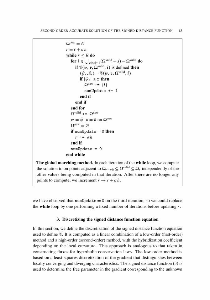
SECOND-ORDER ACCURATE SOLUTION OF THE SIGNED DISTANCE FUNCTION 85
�new=∅
r = ε+ σhwhile r ≤ R do
for i ∈⋃
s:|sd |≤1(�valid+ s)−�valid do
if E(ψ, v, �valid, i) is defined then(ψ i , vi )= E(ψ, v, �valid, i)if |ψ i | ≤ r then�new += {i}numUpdate += 1
end ifend if
end for�valid += �new
ψ = ψ , v = v on �new
�new=∅
if numUpdate= 0 thenr += σh
end ifnumUpdate = 0
end while
The global marching method. In each iteration of the while loop, we computethe solution to on points adjacent to �r−σh ⊆�
valid⊆�r independently of the
other values being computed in that iteration. After there are no longer anypoints to compute, we increment r→ r + σh.
we have observed that numUpdate= 0 on the third iteration, so we could replacethe while loop by one performing a fixed number of iterations before updating r .
3. Discretizing the signed distance function equation
In this section, we define the discretization of the signed distance function equationused to define E. It is computed as a linear combination of a low-order (first-order)method and a high-order (second-order) method, with the hybridization coefficientdepending on the local curvature. This approach is analogous to that taken inconstructing fluxes for hyperbolic conservation laws. The low-order method isbased on a least-squares discretization of the gradient that distinguishes betweenlocally converging and diverging characteristics. The signed distance function (3) isused to determine the free parameter in the gradient corresponding to the unknown

86 PETER SCHWARTZ AND PHILLIP COLELLA
value of 9. This step is similar to that used in [13] and [7]. The high-order methodis based on solving the characteristic form of the equations.
3.1. Least-squares discretization. Given a collection of points p ∈ P ⊂ ZD, wehave the following relationship between the values of the distance function, ψ , andthe gradient:
1h
(ψ(ih)−ψ((i + p)h)
)=− p · ∇ψ + O(h) for p ∈ P . (6)
If P has D linearly independent elements, then we can use (6) as the startingpoint for deriving a first-order accurate method for computing solutions to (3).Given
ψi+ p ≈ ψ((i + p)h) for p ∈ P, (7)
we define ψ ≈ ψ(ih), v ≈ (∇ψ)(ih) as satisfying a least-squares solution to thecoupled equations:
Av =−1h(ψϒ −9), (8)
where the unknown ψ is viewed as a free parameter, to be determined later, and
9 = (ψi+ p1, ψi+ p2, . . . ψi+ pr )T , (9)
A = ( p1, p2, . . . pr )T , (10)
ϒ = (1, 1, . . . 1)T . (11)
Since A is of rank D, the least-squares solution to (8) is given by
v =−(AT A)−1 AT 1h(ψϒ −9)=
ψ−ψ
`n− (ω2− (ω2 · n)n), (12)
where
ω1 =−1h(AT A)−1 ATϒ, ω2 =−
1h(AT A)−1 AT9,
`=1‖ω1‖
, n= ω1`, ψ = (ω2 ·ω1)`2= ψ(ih− `n)+ O(h2).
(13)
We assume here that ω1 is not the zero vector. If ω1 = ω1(P)= 0, then the least-squares problem does not produce a value for ψ , although the expression (12) forthe gradient is still well-defined.
Following [7; 13], the condition ‖v‖2 = 1 leads to a quadratic equation for ψ :
(ψ −ψ)2+ `2‖(ω2− (ω2 · n)n)‖2 = `2. (14)
If (14) has two real roots, we choose the root for which |ψ |> |ψ |. If (14) has noreal roots, we set ψ = ψ .
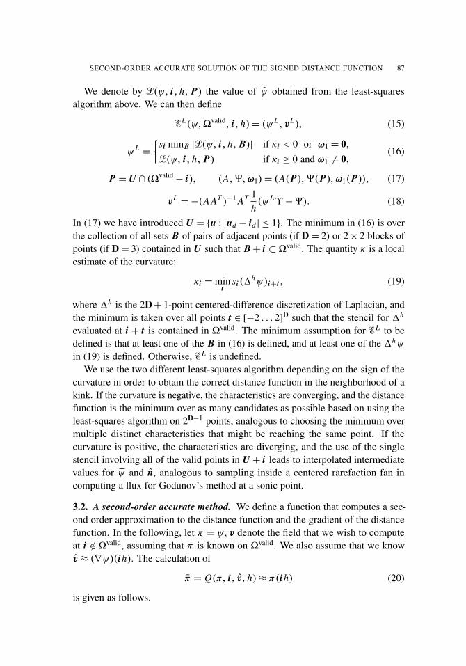
SECOND-ORDER ACCURATE SOLUTION OF THE SIGNED DISTANCE FUNCTION 87
We denote by L(ψ, i, h, P) the value of ψ obtained from the least-squaresalgorithm above. We can then define
EL(ψ,�valid, i, h)= (ψ L , vL), (15)
ψ L=
{si minB |L(ψ, i, h, B)| if κi < 0 or ω1 = 0,L(ψ, i, h, P) if κi ≥ 0 and ω1 6= 0,
(16)
P = U ∩ (�valid− i), (A, 9,ω1)= (A(P),9(P),ω1(P)), (17)
vL=−(AAT )−1 AT 1
h(ψ Lϒ −9). (18)
In (17) we have introduced U = {u : |ud − id | ≤ 1}. The minimum in (16) is overthe collection of all sets B of pairs of adjacent points (if D= 2) or 2× 2 blocks ofpoints (if D= 3) contained in U such that B+ i ⊂�valid. The quantity κ is a localestimate of the curvature:
κi =mint
si (1hψ)i+t , (19)
where 1h is the 2D+ 1-point centered-difference discretization of Laplacian, andthe minimum is taken over all points t ∈ [−2 . . . 2]D such that the stencil for 1h
evaluated at i + t is contained in �valid. The minimum assumption for EL to bedefined is that at least one of the B in (16) is defined, and at least one of the 1hψ
in (19) is defined. Otherwise, EL is undefined.We use the two different least-squares algorithm depending on the sign of the
curvature in order to obtain the correct distance function in the neighborhood of akink. If the curvature is negative, the characteristics are converging, and the distancefunction is the minimum over as many candidates as possible based on using theleast-squares algorithm on 2D−1 points, analogous to choosing the minimum overmultiple distinct characteristics that might be reaching the same point. If thecurvature is positive, the characteristics are diverging, and the use of the singlestencil involving all of the valid points in U + i leads to interpolated intermediatevalues for ψ and n, analogous to sampling inside a centered rarefaction fan incomputing a flux for Godunov’s method at a sonic point.
3.2. A second-order accurate method. We define a function that computes a sec-ond order approximation to the distance function and the gradient of the distancefunction. In the following, let π = ψ, v denote the field that we wish to computeat i /∈ �valid, assuming that π is known on �valid. We also assume that we knowv ≈ (∇ψ)(ih). The calculation of
π = Q(π, i, v, h)≈ π(ih) (20)
is given as follows.

88 PETER SCHWARTZ AND PHILLIP COLELLA
1. Compute x, the first point along the ray {ih− si vδ : δ > 0} that intersects acoordinate plane of gridpoints:
x = ih− si hv
vmax, (21)
where vmax is the component of v whose magnitude is largest, with dmax thecorresponding coordinate direction.
2. Compute a quadratic interpolant in the coordinate plane containing x:
j =⌊
x/h− 12(u− edmax)
⌋, y = x− jh, (22)
π = π j +∑
d 6=dmax
(∂π
∂xdyd +
12∂2π
∂x2d
y2d
)+
∂2π
∂xd1∂xd2
yd1 yd2, (23)
where all of the derivatives are evaluated at jh. The last term in (23) is definedonly for D= 3 and d1 6= d2, d1, d2 6= dmax. We denote by ed the unit vector inthe dth coordinate direction, and u = (1 . . . 1), both elements of ZD.
The derivatives appearing in the sum in (23) are computed using second-orderaccurate centered differences at jh, assuming j , j ± ed
∈ �valid. The mixedderivative is approximated by the average of centered differences:
∂2π
∂xd1∂xd2
≈1N
∑(D2
d1,d2π) j+s/2 (24)
where
(D2d1,d2
π)k+ed1/2+ed1/2 =1h2 (πk+πk+ed1+ed1 −πk+ed1 −πk+ed2 ) (25)
is defined if k, k+ ed1 , k+ ed2 , k+ ed1 + ed2 are all in �valid. The sum in (24) istaken over all s of the form α1ed1 +α2ed2 , α1 =±1, α2 =±1 for which (D2
d1,d2) is
defined, and N is the number of terms in the sum.Given the function Q defined above, we can define a second-order accurate
discretization of the characteristic form of the equations (4) at ih. We iterate twiceto obtain a sufficiently accurate computation of v, computing v at the point i usingthe least-squares algorithm defined in the previous section, and then
v := Q(v, �valid, i, v, h), vH= Q(v, �valid, i, v, h). (26)
We then use vH to compute ψH :
ψH= Q(ψ,�valid, i, vH , h)+ si h
∣∣∣∣ vH
vHmax
∣∣∣∣. (27)
We denote by EH the resulting second-order accurate method for computing ψ, v:
EH (φ, v, �valid, i)≡ (ψH , vH ). (28)

SECOND-ORDER ACCURATE SOLUTION OF THE SIGNED DISTANCE FUNCTION 89
If the low-order method is defined, and the points required for the various evaluationsof Q are defined, then (28) is defined. Otherwise, it is undefined.
3.3. Hybridization. We hybridize the low- and high-order methods based on themagnitude of the curvature. Assuming both EL and EH are defined, we compute
(ψ L , vL)= EL(ψ, v, �valid, i), (29)
(ψH , vH )= EH (ψ, v, �valid, i), (30)
E(ψ, v, �valid, i)=((1− ηi )ψ
H+ ηiψ
L , (1− η2i )v
H+ η2
i vL), (31)
where the hybridization parameter η is given by
ηi =
{1 if h|1hψ |max > C,
h/C |1hψ |max otherwise,(32)
|1hψ |max =maxt|(1hψ)i+t |, (33)
where the range over which the max is taken is the same as in (19). If the high-ordervalue EH (ψ, v, �valid, i) is not defined, but the low-order value is, then
E(ψ, v, �valid, i)= EL(ψ, v, �valid, i). (34)
If the low order value is not defined, then E(ψ, v, �valid, i) is not defined. Theconstant C is an empirically determined parameter, independent of h. In ournumerical experiments, C = 1.
If σ < 1/√
5, and we replace the values of ψ , v on grid points in �r with thoseof a smooth distance function ψe, it is possible to show that, for sufficiently smallh, both EH and EL are defined for all grid points in �r+σh and that
ψHi = ψ
e(ih)+ O(h3), vH=∇ψe(ih)+ O(h3), (35)
ψ Li = ψ
e(ih)+ O(h2), vL=∇ψe(ih)+ O(h), (36)
from which it follows that
E(ψ, v, �valid, i)= (ψe(ih),∇ψe(ih))+ O(h3). (37)
Thus we expect that the global error in our solution will be O(h2). This also explainswhy we use η2, rather than η, to hybridize the gradient calculation. Otherwise, wewould introduce an O(h2) contribution to the error in the gradient at every step,leading to a first-order accurate method for the gradient, and hence for ψ . In theneighborhood of kinks in the level sets of ψ , the value of the curvature is O(h−1),and we will use the low-order method, leading to a first-order accurate method inthe range of influence of the kinks.

90 PETER SCHWARTZ AND PHILLIP COLELLA
3.4. Initialization. We now describe the method we use to provide test problemswith an initial, narrow band three or four cells wide. We are given an initialrepresentation of the surface by a discretized implicit function, from which weconstruct the distance function and the gradient of the distance function an O(h)distance. If the surface is smooth, then our initialization procedure is an O(h2)
approximation to the distance function. If the characteristics cross near the surfaceor the surface is not smooth, then the initialization reduces to a first-order accuratemethod within the range of influence of the kink.
We require some more notation. Denote by (G0φ) the centered differenceapproximation to the gradient of φ. Given a grid location i , let
d =φi
‖(G0φ)i‖.
Let P⊂� denote i and its neighbors. Let
m i =minp∈P‖(G0φ) p‖, Mi =max
p∈P‖(G0φ) p‖. (38)
We choose a nondimensional parameter, ε, independent of h and attempt to detecta discontinuity in the gradient by checking whether M exceeds m by an amountgreater than ε. If so, we make a robust but lower order estimate of the gradient:
if 1−m i
Mi≥ ε, then v = (G0φ) p : ‖(G0φ) p‖ = Mi . (39)
In our numerical experiments, ε = 1/(2√
2). Alternatively, if
1−m i
Mi< ε, (40)
then we define a point,
x0 = ih− d(G0φ)i
‖(G0φ)i‖. (41)
At x0 we biquadratically interpolate an estimate of the gradient v. Finally, weuse root-finding in the direction v to make an estimate of the distance.
4. Numerical results
For our fast marching problems, we always compute the max norm of the error.Where useful, we also compute the L1 and the L2- norm of the solution error.
For a discrete variable, ζ , the max norm is given by
‖ζ‖∞ =maxi|ζi |. (42)

SECOND-ORDER ACCURATE SOLUTION OF THE SIGNED DISTANCE FUNCTION 91
L1 norm rate L2 norm rate L∞ norm rate
4.4566e-02 1.0240e-02 2.1393e-021.0592e-02 2.07 2.4083e-03 2.08 5.9743e-03 1.84
Table 1. Solution error for 2D curve in polar coordinates: h = 1100
and 1200 .
The L p-norm is given by
‖ζ‖p =
(∑i
|(ζi )phD
)1/p
. (43)
For all of the test problems that follow we have used a marching parameter ofσ = 1/(2
√5).
Our first test problem uses the implicit function r = 2 cos 4θ + 7. The domainhas a lower left corner with coordinates (−10,−10,−10) and an upper right cornerwith coordinates (10, 10, 10). The initial bandwidth is approximately six grid cellswide at all resolutions. The final bandwidth is approximately 1.2. Calculations wereperformed on grids with h = 1
100 , 1200 , and 1
400 . Richardson error extrapolation wasused to calculate the results presented in Table 1. The solution is shown in Figure 1and the error is shown in Figure 2.
Figure 1. Curve in polar coordinates.

92 PETER SCHWARTZ AND PHILLIP COLELLA
Figure 2. Error for a curve given in polar coordinates.
Our second test problem has as its zero-level set a surface of revolution. Thedomain has a lower left corner with coordinates (−10,−10,−10) and an upperright corner with coordinates (10, 10, 10). The surface is centered at (0, 0, 0)and obtained by rotating the function r = 2 cos 2θ + 7 around the y-axis. Theinitial bandwidth is approximately six grid cells wide at all resolutions. The finalbandwidth is 1.5. Calculations were performed on grids with h = 1
100 , 1200 , and 1
400 .Richardson error estimation was used to calculate the results presented in Table 2.Slices of the error are presented in Figure 3.
Our next example uses as an implicit function whose zero set is the surface of acube. In this case, to test the robustness of the algorithm we initialized the annularregion to the wrong weak solution of the signed distance function equation. Inparticular, where the characteristics diverge we do not round the corners in theinitial narrow band. Nonetheless our algorithm extends this initial data to a distancefunction.
In this example, the initial band has a diameter of about four grid cells at thecoarse resolution. The final bandwidth is about two and one half times the diameter
L1 norm rate L2 norm rate L∞ norm rate
7.0725 e-01 1.5893 e-02 7.2842e-041.2275 e-01 2.52 3.0446 e-03 2.38 1.813 e-04 2.00
Table 2. Solution error for surface of revolution: h = 1100 and 1
200 .

SECOND-ORDER ACCURATE SOLUTION OF THE SIGNED DISTANCE FUNCTION 93
Figure 3. Slices of the error for a surface of revolution.
of the initial band. Since the only error occurs in places where the gradient isdiscontinuous, we present the max norm of the error in Table 3.
Our final example uses an implicit function generated by taking the union ofparallelepipeds. The zero-set is in the shape of a cube whose corners are removed.Two-dimensional slices are in the shape of a cross. This example tests cases wherecharacteristics meet at a corner as well cases where the characteristics diverge at acorner.
In this problem the domain has a lower left corner with coordinates (0, 0) andan upper right corner with coordinates (1, 1). The initial band is approximately sixcells in diameter at all resolutions. The final bandwidth is 0.15. Since the errorsonly occur in places where the gradient is discontinuous, we present the max normof the error in Table 4. The error is in Figure 4. Three isosurfaces, including thezero level set, are presented in Figures 5–7.
L∞ norm rate
0.004930.00260 0.920.0013 1.0
Table 3. Solution error for distance to a cube: h = 150 , 1
100 , and 1200 .

94 PETER SCHWARTZ AND PHILLIP COLELLA
L∞ norm rate
.00120
.000580 1.05
Table 4. Solution error for distance to a union of parallelepipeds:h = 1
50 , 1100 , and 1
200 .
Figure 4. Slices of the error for a union of parallelepipeds.
Figure 5. The zero isosurface of the union of parallelepipeds.
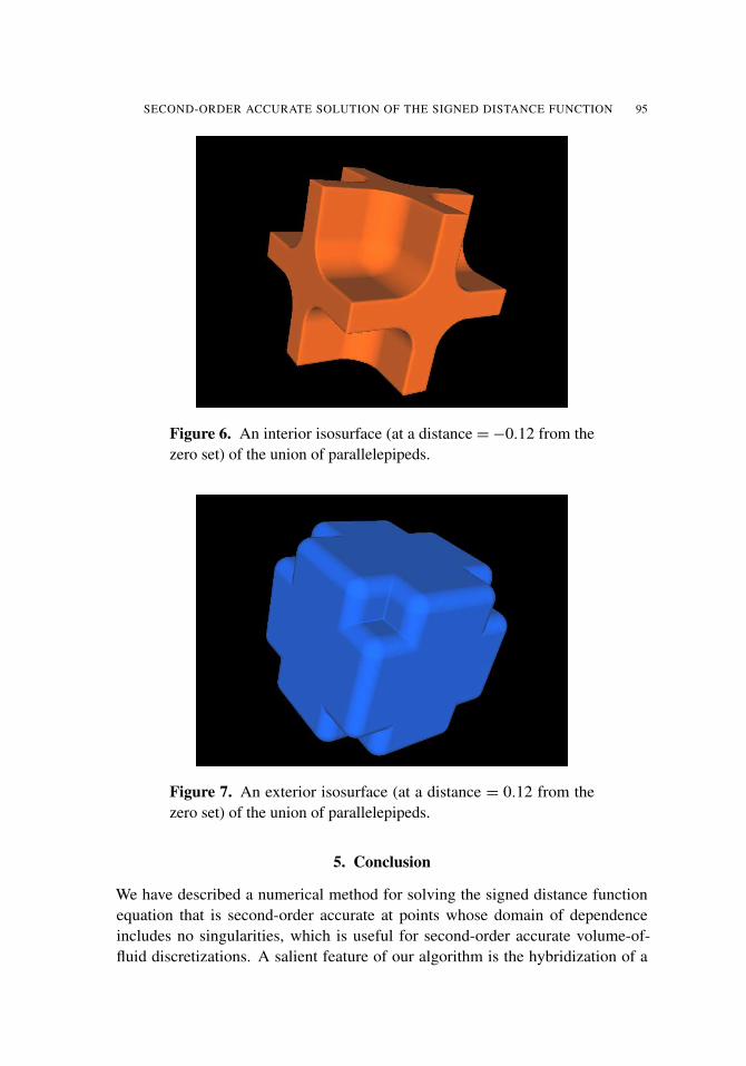
SECOND-ORDER ACCURATE SOLUTION OF THE SIGNED DISTANCE FUNCTION 95
Figure 6. An interior isosurface (at a distance =−0.12 from thezero set) of the union of parallelepipeds.
Figure 7. An exterior isosurface (at a distance = 0.12 from thezero set) of the union of parallelepipeds.
5. Conclusion
We have described a numerical method for solving the signed distance functionequation that is second-order accurate at points whose domain of dependenceincludes no singularities, which is useful for second-order accurate volume-of-fluid discretizations. A salient feature of our algorithm is the hybridization of a

96 PETER SCHWARTZ AND PHILLIP COLELLA
high-order and low-order method, where the choice of hybridization coefficient isbased on a local curvature calculation. The resulting calculation appears to providesolutions that satisfy the entropy condition, correctly distinguishing between thetwo directions of propagation from kinks in the original surface. In addition, we usea marching method that is a good match for adaptive and parallel implementationbased on patch-based domain decomposition, which is the software frameworktypically used for high-performance implementations of block-structured adaptivegrid methods.
Our future work will focus on tracking moving fronts in hyperbolic problems.In these problems, the motion of the interface naturally decomposes into advectionby a vector velocity combined with motion of the interface normal to itself at aknown scalar speed. The importance of the signed distance function equation maybe observed in the special case where the vector velocity is zero and the scalarspeed is spatially constant. In this context, a method of solving the Hamilton–Jacobiequation reduces to a method for computing the signed distance function, up to arelabeling of contours, which leads to the conclusion that numerical methods forHamilton–Jacobi can be no more accurate than the associated solution to the signeddistance function equation. Considering the general front-tracking problem, onemay begin by extending velocities and scalar speeds in the normal direction offthe interface by solving the transport equation, as was done in [1]. Establishedalgorithms for advection may be employed for the velocity component of themotion, while an algorithm for solving the signed distance function equation maybe employed for motion given by scalar speeds.
References
[1] D. Adalsteinsson and J. A. Sethian, The fast construction of extension velocities in level setmethods, J. Comput. Phys. 148 (1999), no. 1, 2–22. MR 99j:65189 Zbl 0919.65074
[2] D. Adalsteinsson and J. A. Sethian, A fast level set method for propagating interfaces, J. Comput.Phys. 118 (1995), no. 2, 269–277. MR 96a:65154 Zbl 0823.65137
[3] D. L. Chopp, Some improvements of the fast marching method, SIAM J. Sci. Comput. 23 (2001),no. 1, 230–244. MR 2002h:65012 Zbl 0991.65105
[4] P. Colella, Volume-of-fluid methods for partial differential equations, Proceedings of an Inter-national Conference on Godunov methods: Theory and Applications (E. F. Toro, ed.), Kluwer,New York, 2001, pp. 161–177. MR 1963590 Zbl 0989.65118
[5] P. Colella, D. T. Graves, B. J. Keen, and D. Modiano, A Cartesian grid embedded bound-ary method for hyperbolic conservation laws, J. Comput. Phys. 211 (2006), no. 1, 347–366.MR 2006i:65142 Zbl 1120.65324
[6] R. Dial, Algorithm 360: Shortest path forest with topological ordering, CACM 12 (1969),632–633.
[7] J. Helmsen, E. G. Puckett, P. Colella, and M. Dorr, Two new methods for simulating pho-tolithography development, Optical Microlithography IX (G. E. Fuller, ed.), SPIE ConferenceProceedings, no. 2726, 1996, pp. 503–555.

SECOND-ORDER ACCURATE SOLUTION OF THE SIGNED DISTANCE FUNCTION 97
[8] S. Kim, An O(N ) level set method for eikonal equations, SIAM J. Sci. Comput. 22 (2001), no. 6,2178–2193. MR 2002h:65126 Zbl 0994.76080
[9] C. Min and F. Gibou, A second order accurate level set method on non-graded adaptive Cartesiangrids, J. Comput. Phys. 225 (2007), no. 1, 300–321. MR 2008g:65128 Zbl 1122.65077
[10] G. Russo and P. Smereka, A remark on computing distance functions, J. Comput. Phys. 163(2000), no. 1, 51–67. MR 2001d:65139 Zbl 0964.65089
[11] P. Schwartz, D. Adalsteinsson, P. Colella, A. Arkin, , and M. Onsum, Numerical computation ofdiffusion on a surface, Proc. Natl. Aca. Sci. 102 (2006), 11151–56.
[12] P. Schwartz, M. Barad, P. Colella, and T. Ligocki, A Cartesian grid embedded boundary methodfor the heat equation and Poisson’s equation in three dimensions, J. Comput. Phys. 211 (2006),no. 2, 531–550. MR 2006e:65194 Zbl 1086.65532
[13] J. A. Sethian, A fast marching level set method for monotonically advancing fronts, Proc. Nat.Acad. Sci. USA 93 (1996), no. 4, 1591–1595. MR 97c:65171 Zbl 0852.65055
[14] , Fast marching methods, SIAM Rev. 41 (1999), no. 2, 199–235. MR 2000m:65125Zbl 0926.65106
[15] M. Sussman, P. Smereka, and S. Osher, A level set approach for computing solutions to incom-pressible two-phase flow, J. Comput. Phys. 114 (1994), 146–159. Zbl 0808.76077
Received February 5, 2008. Revised July 9, 2009.
PETER SCHWARTZ: [email protected] Berkeley National Laboratory, 1 Cyclotron Road, MS 50A-1148MS 50A-1148,Berkeley CA 94720, United Stateshttp://seesar.lbl.gov/ANAG/staff/schwartz/index.html
PHILLIP COLELLA: [email protected] Numerical Algorithms Group, Lawrence Berkeley National Laboratory,1 Cyclotron Road MS 50A-1148, Berkeley CA 94720, United States


COMM. APP. MATH. AND COMP. SCI.Vol. 5, No. 1, 2010
ON THE SECOND-ORDER ACCURACY OFVOLUME-OF-FLUID INTERFACE RECONSTRUCTIONALGORITHMS: CONVERGENCE IN THE MAX NORM
ELBRIDGE GERRY PUCKETT
Given a two times differentiable curve in the plane, I prove that — using onlythe volume fractions associated with the curve — one can construct a piecewiselinear approximation that is second-order in the max norm. I derive two parame-ters that depend only on the grid size and the curvature of the curve, respectively.When the maximum curvature in the 3 by 3 block of cells centered on a cellthrough which the curve passes is less than the first parameter, the approxima-tion in that cell will be second-order. Conversely, if the grid size in this blockis greater than the second parameter, the approximation in the center cell can beless than second-order. Thus, this parameter provides an a priori test for whenthe interface is under-resolved, so that when the interface reconstruction methodis coupled to an adaptive mesh refinement algorithm, this parameter may be usedto determine when to locally increase the resolution of the grid.
1. Introduction
In this article I study the interface reconstruction problem for a volume-of-fluidmethod in two space dimensions. Let � ∈ R2 denote a simply connected domainand let z(s)= (x(s), y(s)), where s is arc length, denote a curve in�. The interfacereconstruction problem is to compute an approximation z(s) to z(s) in � using onlythe volume fractions due to z on the grid. I define volume fractions and discussthis problem in more detail in Section 1.1 below.
Let L be a characteristic length of the problem. Cover � with a grid consistingof square cells each of side 1x ≤ L and let
h =1xL
(1)
MSC2000: 76-04, 65M06, 65M12, 76M20, 76M25.Keywords: volume-of-fluid, piecewise linear interface reconstruction, fronts, front reconstruction,
two-phase flow, multiphase systems, underresolved computations, adaptive mesh refinement,computational fluid dynamics, LVIRA, ELVIRA.
Sponsored by the U.S. Department of Energy (Mathematical, Information, and Computing SciencesDivision, contracts DE-FC02-01ER25473 and DE-FG02-03ER25579).
99

100 ELBRIDGE GERRY PUCKETT
be a dimensionless parameter that represents the size of a grid cell as a nondimen-sional quantity. Note that h is bounded above by 1. This ensures that second-orderaccurate methods, which have O(h2) error, will be more accurate than first-orderaccurate methods, which have O(h) error. For the remainder of this article it willbe understood that quantities such as the arc length s and the radius of curvatureR are also nondimensional quantities obtained by division by L as in (1) and thatthe curvature κ has been nondimensionalized by dividing by 1/L .
In this article I prove that a piecewise linear volume-of-fluid interface reconstruc-tion method will be a second-order accurate approximation to the exact interfacez(s)= (x(s), y(s)) in the max norm provided the following four conditions hold:
I. The interface z is two times continuously differentiable: z(s) ∈ C2 (�).
II. The maximum valueκmax =max
s|κ(s)| (2)
of the curvature κ(s) of z(s) satisfies1
κmax ≤ Cκ ≡min{Ch h−1,
(√h)−1}
, (3)
where Ch is a constant that is independent of h and is defined by
Ch ≡
√2− 1
4√
3. (4)
III. In each cell Ci j that contains a portion of the interface, the slope mi j of thepiecewise linear approximation
gi j (x)= mi j x + bi j (5)
to the interface in that cell is given by
mi j =Si+α − Si+β
α−βfor α, β = 1, 0,−1 with α 6= β, (6)
where Si+α and Si+β denote two distinct column sums of volume fractionsfrom the 3× 3 block of cells Bi j surrounding the cell Ci j .2 The column sumsSi−1, Si , and Si+1 are defined and described in more detail in Section 1.3.
IV. The column sums Si+α and Si+β in (6) are sufficiently accurate that the slopemi j defined in (6) is a first-order accurate approximation to g′(xc), where xc
is the center of the bottom edge of the cell Ci j .
1It is only necessary that the maximum curvature of the interface satisfy this condition in a neigh-borhood of the cell Ci j in which one wishes to reconstruct the interface. For example, in the 3× 3block of cells Bi j centered on Ci j .
2I will usually omit the subscript i, j when writing the piecewise linear approximation g definedin (5) and simply write g(x) instead of gi j (x). Similarly, when no confusion is likely to arise, I willdrop the subscript i, j from the slope m and the y-intercept b and simply write g(x)= m x + b.

SECOND-ORDER ACCURACY OF VOF INTERFACE RECONSTRUCTION 101
Section 3 is devoted to proving that if condition (3) above is satisfied, one canalways find an orientation of the 3×3 block of cells (say, after rotating by a multipleof 90 degrees) so that there are two column sums Si+α and Si+β , both in the sameorientation of the 3× 3 block, satisfying the condition in item IV above. Note thathere I do not provide an algorithm for determining which orientation of the 3× 3block of cells is the correct one to use or, given a correct orientation, how to findthe two column sums to use in (6). What I do prove is that if the interface satisfiesEquation (3), then one can find an orientation of the 3× 3 block of cells that hastwo distinct column sums Si+α and Si+β such that the slope mi j obtained in (6)is a first-order accurate approximation to g′(xc) and hence, g is a second-orderaccurate approximation to g in the max norm as illustrated in Figure 1.3
xi−2 xi−1 xi xi+1xc = 0|yj−2
yj−1
yj
yj+1
yc = 0 −g(x) = tanh(x)
(xl, yl)
(xr, yr)
g(x) = m x + b
Figure 1. In this example the interface is g(x)= tanh x . All threecolumn sums are exact (in the sense of Section 1.3), but for theinverse function x = g−1(y) only the center column sum is exact.Also plotted is the linear approximation g(x) = m x + b in thecenter cell produced by the volume-of-fluid interface reconstruc-tion algorithm when the slope m is chosen as half the differencebetween the first and third column sums. The main result of thispaper is that |g(x)− g(x)| ≤ Ch2 for all x ∈ [xi−1, xi ] providedthat the slope m is defined in the manner described in Section 1.3.
3In this particular example all three of the column sums Si−1, Si and Si+1 are exact. Conse-quently, Theorem 23 in Section 4 implies any two of them can be used in (6) and that the resultingslope m = g′(xc) is a first-order accurate approximation to g′(xc), regardless of whether one choosesthe slope to be m = (Si − Si−1), m = (Si+1− Si−1)/2, or m = (Si+1− Si ).

102 ELBRIDGE GERRY PUCKETT
A variety of algorithms have been proposed for determining the correct columnsums to use to determine the approximate slope via Equation (6). I refer the inter-ested reader to [6; 7; 11; 14; 22; 23; 25; 37] for further information.
Finally, I would like to emphasize that the criteria in (3) provides an a priori testto determine when a given computation of the interface is well-resolved; namely,the computation is well-resolved whenever
h ≤ Hmax =min{Ch (κmax)−1 , (κmax)
−2}. (7)
This will enable researchers who employ block structured adaptive mesh refine-ment to model the motion of an interface [30; 31; 33; 34] to compute an approx-imation to the curvature of the interface in each cell and then check to see if theconditions in (7) are satisfied in order to determine if the computation is under-resolved in that cell. Cells in which h > Hmax are then tagged for refinement. Inthis regard I note that Sussman and Ohta [32] have developed second- and fourth-order accurate volume-of-fluid algorithms for computing the curvature from thevolume fraction information.
1.1. A detailed statement of the problem. Suppose that I am given a simply con-nected computational domain � ∈ R2 that is divided into two distinct regions �d
and �l so that �=�d ∪�l . I will refer to �d as the “dark” fluid4 and to �l as the“light” fluid. Let z(s) = (x(s), y(s)), where s is arc length, denote the interfacebetween these two fluids. Cover � with a uniform square grid of cells, each withside h, and let 3i j denote the fraction of dark fluid in the (i, j)-th cell. Eachnumber 3i j satisfies 0≤3i j ≤ 1 and is called the volume fraction (of dark fluid)in the (i, j)-th cell.5 Note that
0<3i j < 1 (8)
if and only if a portion of the interface z(s) lies in the (i, j)-th cell and that 3i j = 1(resp. 3i j = 0) if the i, j cell only contains dark (resp. light) fluid.
In this paper I consider the following problem. Given only the collection of vol-ume fractions 3i j in the grid covering � I wish to reconstruct z(s); that is, to finda piecewise linear approximation z to z. Furthermore, the approximate interface zmust have the property that the volume fractions 3i j due to z are identical to the
4Although these algorithms have historically been known as “volume-of-fluid” methods, they arefrequently used to model the interface between any two materials, including gases, liquids, solidsand any combination thereof [8; 16; 17; 18]. However, when analyzing the method, the conventionis to refer to the two materials as fluids.
5Even though in two dimensions 3i j is technically an area fraction, the convention is to refer toit as a volume fraction.

SECOND-ORDER ACCURACY OF VOF INTERFACE RECONSTRUCTION 103
original volume fractions 3i j ; that is,
3i j =3i j for all cells Ci j . (9)
An algorithm for finding such an approximation is known as a volume-of-fluidinterface reconstruction method. The property that 3i j = 3i j is the principalfeature that distinguishes volume-of-fluid interface reconstruction methods fromother interface reconstruction methods. It ensures that the computational value ofthe total volume of each fluid is exact. In other words, all volume-of-fluid interfacereconstruction methods are conservative in that they conserve the volume of eachmaterial in the computation. When the underlying numerical method is a conser-vative finite difference method this can be essential since, for example, in order toobtain the correct shock speed it is necessary for all of the conserved quantitiesto be conserved by the underlying numerical method; for example, see [5; 17; 18;26]. More generally, a necessary condition for the numerical method to convergeto the correct weak solution of the underlying partial differential equation (PDE)is that all of the quantities that are conserved in the PDE must be conserved by thenumerical method [15].
Volume-of-fluid methods have been used by researchers to track material inter-faces since at least the early 1970s (see [20; 21], for example), and a variety of suchalgorithms have been developed for modeling everything from flame propagation[3] to curvature and solidification [4]. In particular, the problem of developinghigh-order accurate volume-of-fluid methods for modeling the curvature and sur-face tension of an interface has received much attention [1; 2; 4; 10; 13; 24].Volume-of-fluid methods were among the first interface tracking algorithms to beimplemented in codes originally developed at the U.S. National Laboratories andsubsequently released to the general public which are capable of tracking fluidinterfaces in a variety of complex fluid flow problems [9; 12; 19; 35; 36]).
In this paper I do not consider the related problem of approximating the move-ment of the interface in time, for which one would use a volume-of-fluid advectionalgorithm. See [23; 27; 28] for a detailed description and analysis of several suchalgorithms. In the present paper I only consider the accuracy that one can obtainwhen using a volume-of-fluid interface reconstruction algorithm to approximate agiven stationary interface z(s).
1.2. Basic assumptions and definitions. Unless explicitly stated otherwise, I willalways assume that the exact interface z(s) = (x(s), y(s)) is twice continuouslydifferentiable: z ∈ C2(�). In particular, the derivatives x(s), y(s), x(s) and y(s)exist and are continuous. I also assume that the curvature κ(s) of the interface z(s)is bounded in �, so that there always exists a constant κmax independent of s suchthat (2) holds.

104 ELBRIDGE GERRY PUCKETT
By the center cell Ci j I mean the square with side h that contains a portion of theinterface z(s)= (x(s), y(s)) for s in some interval, say s ∈ (sl, sr ). In what followsI will consider the 3× 3 block of square cells Bi j — each with side h, surroundingthe center cell as shown, for example, in Figure 1. Unless I note otherwise, I willdenote the coordinates of the vertical edges of the cells in the 3× 3 block Bi j
centered on the cell Ci j by xi−2, xi−1, xi and xi+1 and the horizontal edges of thecells in Bi j by y j−2, y j−1, y j , y j+1 as shown, for example, in Figure 1. It willalways be the case that
xi+1− xi = h, xi − xi−1 = h,
y j+1− y j = h, y j − y j−1 = h,
and so on, where h is the (nondimensional) grid size.
1.3. The column sums. The volume fraction3i j in the (i, j)-th cell Ci j is a nondi-mensional way of storing the volume of dark fluid in that cell. Consider the columnconsisting of Ci j and the cells immediately above and below Ci j . The column sum
Si ≡
j+1∑j ′= j−1
3i j ′
is a nondimensional way of storing the total volume of dark fluid in those threecells. In order to approximate the portion of the interface g(x) lying in the (i, j)-thcell Ci j , I will use the three column sums in the 3× 3 block of cells Bi j that haveCi j in its center to compute the slope m of the piecewise linear approximation g(x)to g(x) (for example, see Figure 1). I use Si−1 to denote the column sum to theleft of Si and Si+1 to denote the column sum to the right of Si , so that
Si−1 ≡
j+1∑j ′= j−1
3i−1, j ′, Si+1 ≡
j+1∑j ′= j−1
3i+1, j ′ . (10)
Now consider an arbitrary column consisting of three cells with left edge x = xi
and right edge x = xi+1. Furthermore, assume that the interface can be written as afunction y = g(x) on the interval [xi , xi+1]. Assume also that the interface entersthe column through its left edge and exits the column through its right edge anddoes not cross the top or bottom edges of the column, as is the case with all threecolumns in the example shown in Figure 1. Then the total volume of dark fluid thatoccupies the three cells in this particular column and lies below the interface g(x)is equal to the integral of g over the interval [xi , xi+1]. This leads to the followingrelationship between the column sum and the normalized 6 volume of dark fluid in
6The normalized volume is the nondimensional quantity obtained by dividing the integral of g(x)over the interval [xi , xi+1] by h2.

SECOND-ORDER ACCURACY OF VOF INTERFACE RECONSTRUCTION 105
the column:
Si ≡
j+1∑j ′= j−1
3i j ′ =1h2
∫ xi+1
xi
(g(x)− y j−2 h
)dx . (11)
I will use the phrase the i-th column sum Si is exact whenever (11) holds, and Iwill refer to integrals such as the one on the right in (11) as the normalized integralof g in that column.
Given the 3× 3 block of cells surrounding a cell Ci j that contains a portiony = g(x) of the interface, most of the important results in this paper are based onhow well the column sums Si−1, Si and Si+1 approximate the normalized integralof g in that particular column. This is because the slope mi j of the piecewise linearapproximation to g in Ci j will be the divided difference of two of these columnsums; that is, mi j is chosen to be one of the three quantities
mli j = Si − Si−1, mc
i j =12(Si+1− Si−1), mr
i j = Si+1− Si . (12)
In particular, if two of the column sums Si+α and Si+β where α, β = 1, 0,−1 andα 6= β are exact, then the slope
mi j =
(Si+α − Si+β
)(α−β)
(13)
will produce a piecewise linear approximation g(x) to the portion of the interfaceg(x) in Ci j that is second-order accurate in the max norm as shown, for example,in Figure 1.
In order to see why this will be the most accurate choice for the approximateslope mi j , consider the case when the block Bi j has two exact column sums asshown in Figure 2. In this example the interface is a line g(x)= m x + b. In thisparticular orientation of the 3× 3 block of cells g has two exact column sums;namely, the sums in the first and second columns. It is easy to check that
m =1h2
∫ xi
xi−1
( g(x)− y j−2h)dx
−1h2
∫ xi−1
xi−2
( g(x)− y j−2h)dx = (Si − Si−1)= mli j ,
where Si denotes the column sum associated with the interval [xi−1, xi ] and Si−1
denotes the column sum associated with the interval [xi−2, xi−1].In this example, the divided difference ml
i j of the column sums Si−1 and Si isexactly equal to the slope m of the exact interface. It is always the case that whenthe exact interface is a line one can find an orientation of the 3× 3 block of cellssuch that at least one of the divided differences of the column sums in (12) is exact.

106 ELBRIDGE GERRY PUCKETT
xi−2 xi−1 xi xi+1
yj−2
yj−1
yj
yj+1
g(x)
(xl, yl)
(xr, yr)
Figure 2. Here the interface is a line, g(x) = m x + b, havingtwo exact column sums (those in the first and second columns).The slope ml
i j from (12) is then exactly equal to the slope m of theinterface: ml
i j = m. Whenever the exact interface is a line, one canfind an orientation of the 3× 3 block of cells such that at least oneof the divided differences of the column sums in (12) is exact.
For example, in the case shown in Figure 2 one could rotate the 3×3 block of cells90 degrees clockwise and in this orientation the correct slope to use when formingthe piecewise linear approximation g(x)= mi j + bi j would be mi j = mr
i j , whichagain would be exactly equal to the slope m of the exact interface.
However, as I will show in Section 3, there are some instances in which theinterface satisfies (3) but the center column sum Si is not exact. Much of the workin Section 3 is devoted to showing that when the interface satisfies (3), the centercolumn sum Si are exact to O(h):
1h2
∫ xi+1
xi
(g(x)− y j−2h)dx − Si = Ch,
where C > 0 is a constant that is independent of h. Then, in Section 4, I prove thatthis is sufficient to still obtain second-order accuracy in the max norm.
I am now ready to finish the description of the volume-of-fluid interface recon-struction algorithms that I study in this article. Given an arbitrary interface z in thedomain �, I choose an orientation of the 3× 3 block of cells such that at least twoof the column sums are sufficiently accurate that one of the divided differences in

SECOND-ORDER ACCURACY OF VOF INTERFACE RECONSTRUCTION 107
(12) satisfies|mi j − g′(xc)| ≤ Ch, (14)
where C is a constant that is independent of h. In this article I prove that, providedthe condition in (3) is satisfied, it is possible to find such an orientation.
1.4. A brief overview of the structure of this article. In the next section I beginby proving several lemmas that lead to Theorem 6, which states that if
h ≤ Ch (κmax)−1 (15)
where Ch is defined in (4), then the interface can be written as a function of one ofthe coordinate variables in terms of the other on an interval [a, b] with |b−a | ≥ 4 h.This ensures that, given a cell Ci j that contains a portion of the interface, I canalways find a 3× 3 block of cells centered on the cell Ci j in which I can write theinterface as a function of one of the variables in terms of the other; for example,y = g(x). To achieve this, it may be necessary to rotate the 3× 3 block of cellscentered on Ci j by 90, 180, or 270 degrees and/or reflect the coordinates aboutone of the coordinate axes: x →−x or y→−y. No other coordinate transfor-mations besides one of these three rotations and a possible reversal of one or bothof the variables x→−x and/or y→−y are required in order for the algorithmsstudied in this article to converge to the exact interface as h→ 0. Furthermore,these coordinate transformations are only used to determine a first-order accurateapproximation to the slope of the tangent to the interface z in the current cell ofinterest, or equivalently, a first-order accurate approximation m to g′(xc) in thecenter cell, as shown, for example, in Figure 1. The grid covering the domain �always remains the same.
In particular, if one is using the interface reconstruction algorithm as part of anumerical method to solve a more complex problem than the one posed here (forexample, the movement of a fluid interface where the fluid flow is a solution of theEuler or Navier–Stokes equations), it is not necessary to perform these coordinatetransformations on the underlying numerical fluid flow solver. Therefore, unlessnoted otherwise, in what follows I will always write y = g(x) and denote thecoordinates of the edges of the cells in the 3× 3 block by x = xi−2, xi−1, xi , xi+1
and y = y j−2, y j−1, y j , y j+1, it being implicitly understood that a transformationof the coordinate system as described above may have been performed in order forthis representation of the interface to be valid, and that I may have interchangedthe names of the variables x and y in order to write the interface as y = g(x).
In Section 2 I will also prove that in the (possibly transformed) coordinates thefunction y = g(x) that represents the interface satisfies
|g′(x)| ≤√
3, maxx|g′′(x)| ≤ 8κmax. (16)

108 ELBRIDGE GERRY PUCKETT
These inequalities are a part of Theorem 6. I use these bounds to prove several ofthe results in Sections 3 and 4.
In Section 3 I prove that if h satisfies
h ≤max{Ch(κmax)−1, (κmax)
−2},
then, using one of the transformations described above, I can find a coordinateframe in which there are at least two columns with column sums Si+α and Si+β inthe 3× 3 block of cells Bi j centered on the cell Ci j which contains the portion ofthe interface of interest, such that their divided difference,
mi j =(Si+α − Si+β)
(α−β)for α, β =−1, 0, 1 and α 6= β,
satisfies (14).In Section 4 I use this result to prove Theorem 24, which is the main result of
this paper. Namely that g(x) is a second-order accurate approximation to g(x) inIi in the max norm:
| g(x)− gi j (x) | ≤( 50
3 κmax+CS)h2 for all x ∈ Ii = [xi−1, xi ].
Here CS is a constant that is independent of h and the approximate interface gi j (x)is being constructed in the center cell Ci j = [xi−1, xi ] × [y j−1, y j ] of the 3× 3block of cells Bi j that contains the portion of the interface that is of interest, asshown, for example, in Figure 1. A corollary of this result is that when the size ofthe computational grid h is too large
h ≥ Hmax, (17)
where Hmax is defined in (7), then the convergence rate may be less than second-order. Thus, (17) may be used as a criterion for predicting when the computationof the interface may be under-resolved.
2. The first constraint on the grid size h
The principle purpose of this section is to show that for a given interface z(s) witha maximum curvature κmax there exists a value of the grid size h = hmax such thatthe interface can be written as a function of one of the coordinate variables in termsof the other in any given 3× 3 block of cells Bi j of side h ≤ hmax centered on acell Ci j that contains a portion of the interface. The main result in this section isTheorem 6, in which I derive the constraint
h ≤ hmax ≡ Ch(κmax)−1, (18)
where Ch is the constant defined in (4). I also prove that in the same 3× 3 blockof cells Bi j centered on the cell Ci j the bounds in (16) hold.

SECOND-ORDER ACCURACY OF VOF INTERFACE RECONSTRUCTION 109
The constraint in (18) is not sufficient to guarantee that the volume-of-fluidinterface reconstruction algorithm will be second-order accurate in the limit ash→ 0. In Section 3 below, I will show that this requires a more stringent constrainton h, namely
h ≤ (κmax)−2.
Suppose that I am interested in a neighborhood of the point z(s0) = (x(s0),y(s0))≡ (x0, y0) on the interface7 and at this point I have
x2(s0)≥12 . (19)
I will now show that in some neighborhood of the point (x0, y0) I can representthe interface (x(s), y(s)) as the single valued function y(s) = g(x(s)). Then, inLemma 4 I will answer the question: Over how large an interval [xl, xr ] wherexl < x0 = x(s0) < xr is this representation of the interface valid? I will nowproceed to address this question.
Let sl < sr8 chosen such that sl is the largest number less than s0 and sr is the
smallest number greater than s0 such that
x2(s)≥ 14 for all s ∈ [sl, sr ]. (20)
Given that at the point z(s0) the inequality in (19) holds there are two possibilitiesfor the point z(sl) (resp. z(sr )).
(1) At the point z(sl) (resp. z(sr )) I have
x2(sl)=14
(resp. x2(sr )=
14
). (21)
In this case I can estimate the size of the interval [xl, x0] (resp. [x0, xr ]) overwhich I can represent the interface as a function of one of the coordinatevariables in terms of the other, say y = g(x), and bound the first and secondderivatives of this function. All of these estimates will be in terms of onequantity; namely, κmax, the maximum curvature of the interface.
(2) For all s < s0 (resp. s > s0) I have
x2(s) > 14 ,
and at some point z(sl) (resp. z(sr )) the interface z(s) intersects the boundaryof the computational domain �. In this case the bound in (2) holds from thepoint x0 up to the point xl (resp. xr ) on the boundary. In this case, I can
7In this section, and this section only, x0 and y0 denote a point on the interface z(s0) =(x(s0), y(s0))≡ (x0, y0) rather than the location of one of the grid lines in the 3× 3 block of cells.
8Without loss of generality I can assume that x(s) increases with increasing s, since otherwisethe change of variables s→−s is also a parametrization of the interface by arc length for which x(s)increases with increasing s.

110 ELBRIDGE GERRY PUCKETT
express the interface as a function such as y = g(x) from x0 ∈ [−h/2, h/2] allthe way to the boundary on the left (resp. right); that is, in the interval [xl, x0]
(resp. in the interval [x0, xr ]).
Note that since I have assumed that the domain � is bounded and that either theinterface enters and exits the domain across the boundary or it is a closed curve in�, these are the only two possibilities. For if the interface is a closed curve, suchas a circle, it must be the case that eventually x(s)→ 0.
In either case, there is an interval [xl, xr ] upon which I can express the interfaceas a function y = g(x) and upon which all of the bounds that I prove below willhold. The only difference between cases (1) and (2) above is that in case (2) oneor both of the points xl and xr lie on the boundary of the domain.
Since, for the purposes of the proving the lemmas and theorems below, I donot know a priori the distance from x0 to the boundary, for the remainder of thissection I will assume that case (1) above holds and proceed to estimate the sizeof the intervals [xl, x0] and [x0, xr ] in terms of the bound κmax on the curvatureof the interface. This will allow me to explicitly estimate the size of the interval[xl, xr ] containing the point of interest (x0, y0)≡ (x(s0), y(s0)) over which I canexpress the interface as a function y = g(x) and prove explicit bounds on the firstand second derivatives of g.
Remark 1. If the inequality in (19) fails to hold at the point z(s0) at which I wishto reconstruct the interface, then y2(s0)≥
12 instead, since s is arc length and hence
x2(s)+ y2(s)= 1. In this case I instead choose y to be the independent variableand the same analysis will produce the same estimates throughout. Therefore, inall of what follows x will denote the independent variable, it being understood thatin some cases y is the correct variable to choose.
Remark 2. The choice of the constant 12 in (19) and the constant 1
4 in (21) isarbitrary. One could have chosen instead any two constants C1 and C2 that satisfyC1 > C2 > 0 in the proof of Lemma 3. The lemma will continue to hold, but thevalues of the constants Ch and hmax in Theorem 6 below will change. In otherwords, all of our results will remain true, albeit with different constants.
I begin by finding a bounds on the second derivatives x(s) and y(s) of thefunctions x(s) and y(s) in terms of the global bound κmax on the curvature ofthe interface. I will use these bounds to estimate the size of the intervals [xl, x0]
and [x0, xr ] in terms of the intervals [sl, s0] and [s0, sr ], respectively, in the twosubsequent lemmas.
Lemma 3 (A bound on x(s) and y(s)). Suppose that I am given a point z(s0) =
(x(s0), y(s0)) on the interface at which the inequality
y2(s)≤ 12 ≤ x2(s) (22)

SECOND-ORDER ACCURACY OF VOF INTERFACE RECONSTRUCTION 111
holds. Let sl < s0 be the largest number less than s0 and sr > s0 be the smallestnumber greater than s0 such that
14 ≤ x2(s)
(and hence y2(s)≤ 3
4
)for all s ∈ [sl, sr ] . (23)
Then|x(s)| ≤
√3
2 κmax for all s ∈ [sl, sr ] . (24)
Similarly, if the roles of x(s) and y(s) are reversed in the inequalities in Equations(22) and (23) above, then I have
|y(s)| ≤√
32 κmax for all s ∈ [sl, sr ] . (25)
Proof. To begin, recall that since the parameter s is arc length,
x2(s)+ y2(s)= 1 (26)
holds for all s, and hence the curvature κ(s) can be written as
κ(s)= x(s)y(s)− y(s)x(s) (27)
(see [29, page 555]). Differentiating (26) with respect to s I find that
x(s)x(s)=−y(s)y(s), (28)
or equivalently−x2(s)x(s)= y(s)x(s)y(s). (29)
Multiplying (27) by y(s) I have
y(s)κ(s)= y(s)x(s)y(s)− y2(s)x(s), (30)
and thus, using (29) in (30), I obtain
y(s)κ(s)=−x(s)(x2(s)+ y2(s))=−x(s). (31)
Combining (31) and (23) I obtain the following bound on x(s) in terms of thebound κmax on the curvature κ(s),
|x(s)| = |y(s)κ(s)| ≤ |y(s)|κmax ≤√
32 κmax.
One can use an identical argument to prove the bound on y(s) in (25). �
In the next lemma I explicitly demonstrate how the size of the intervals [xl, x0] and[x0, xr ] depend on the size of the intervals [sl, s0] and [s0, sr ] respectively. In thelemma after that I provide an explicit relationship between the size of the intervals[sl, s0] and [s0, sr ] the bound κmax in (2) on the curvature of the interface.

112 ELBRIDGE GERRY PUCKETT
Lemma 4. Let z(s0) = (x(s0), y(s0)) be a point on the interface at which the in-equality
y2(s0)≤12 ≤ x2(s0)
holds, and let sl < s0 be the greatest number less than s0 and sr > s0 the smallestnumber greater than s0 such that
14 ≤ x2(s) for all s ∈ [sl, sr ]. (32)
Then, letting xl ≡ x(sl), x0 ≡ x(s0), and xr ≡ x(sr ), the following inequalities hold:
12 |s0− sl | ≤ |x0− xl | ≤ |s0− sl |,
12 |sr − s0| ≤ |xr − x0| ≤ |sr − s0|. (33)
Proof. I prove that the inequalities involving sl are true. The proof of the other pairof inequalities is identical. By the mean-value theorem I have
x0− xl = x(s)(s0− sl) for some s ∈ (s0, sl). (34)
Since both (26) and (32) hold I have 14 ≤ x2(s)≤ 1 for all s ∈ [sl, sr ], and hence
12 ≤ |x(s)| ≤ 1 for all s ∈ [sl, sr ]. (35)
Combining (34) and (35) I obtain
12 |s0− sl | ≤ |x0− xl | ≤ |s0− sl |,
as claimed. �
But how large are the intervals [sl, s0] and [s0, sr ] in terms of the physical coor-dinates x and y? The following lemma addresses this question.
Lemma 5. Let z(s0) = (x(s0), y(s0)) be a point on the interface at which the in-equality
y2(s0)≤12 ≤ x2(s0) (36)
holds. If sl < s0 is the greatest number less than s0 and sr > s0 is the smallestnumber greater than s0 such that
x2(sl)=14 = x2(sr ), (37)
then the distances |sr − s0| and |s0− sl | satisfy
|s0− sl | ≥
√2− 1√
3(κmax)
−1 , |sr − s0| ≥
√2− 1√
3(κmax)
−1 . (38)
Proof. I will prove the first inequality; the proof of the second is identical. Letxl = x(sl) and x0= x(s0). By the mean-value theorem I have x0− xl = x(s)(s0−sl)
for some s ∈ (s0, sr ), and hence
|x0− xl | = |x(s)||s0− sl | ≤√
32 |s0− sl |κmax, (39)
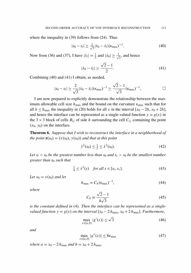
SECOND-ORDER ACCURACY OF VOF INTERFACE RECONSTRUCTION 113
where the inequality in (39) follows from (24). Thus
|s0− sl | ≥2√
3|x0− xl |(κmax)
−1. (40)
Now from (36) and (37), I have |xl | =12 and |x0| ≥
1√
2, and hence
|x0− xl | ≥
√2− 12
. (41)
Combining (40) and (41) I obtain, as needed,
|s0− sl | ≥2√
3|x0− xl |(κmax)
−1≥
√2− 1√
3(κmax)
−1, �
I am now prepared to explicitly demonstrate the relationship between the max-imum allowable cell size hmax and the bound on the curvature κmax such that forall h ≤ hmax the inequality in (20) holds for all x in the interval [x0− 2h, x0+ 2h],and hence the interface can be represented as a single-valued function y = g(x) inthe 3× 3 block of cells Bi j of side h surrounding the cell Ci j containing the point(x0, y0) on the interface.
Theorem 6. Suppose that I wish to reconstruct the interface in a neighborhood ofthe point z(s0)= (x(s0), y(s0)) and that at this point
y2(s0)≤12 ≤ x2(s0). (42)
Let sl < s0 be the greatest number less than s0 and sr > s0 be the smallest numbergreater than s0 such that
14 ≤ x2(s) for all s ∈ [sl, sr ]. (43)
Let x0 = x(s0) and lethmax = Ch(κmax)
−1, (44)
where
Ch ≡
√2− 1
4√
3(45)
is the constant defined in (4). Then the interface can be represented as a single-valued function y = g(x) on the interval [x0− 2 hmax, x0+ 2 hmax]. Furthermore,
maxx∈[a,b]
|g′(x)| ≤√
3 (46)
andmax
x∈[a,b]|g′′(x)| ≤ 8κmax (47)
where a = x0− 2 hmax and b = x0+ 2 hmax.

114 ELBRIDGE GERRY PUCKETT
Remark 7. As a consequence of this theorem, if the point z0 = z(s0) lies in somecell Ci j of side h ≤ hmax, then the interface can be represented as a single-valuedfunction y = g(x) throughout the 3×3 block Bi j of square cells of side h surround-ing Ci j and the bounds in (46) and (47) hold throughout Bi j .
Remark 8. It is apparent that interchanging the roles of x(s) and y(s) in Lem-mas 3–5 and Theorem 6 above will show that the interface can be represented asa single-valued function x = G(y) throughout the 3× 3 block Bi j of square cellsof side h surrounding Ci j and the bounds in (46) and (47) hold throughout the Bi j
with x replaced by y and g replaced by G.
Proof. Let xl = x(sl) and xr = x(sr ). Since, by the implicit function theorem, theinterface can be represented as a single-valued function y = g(x) on any intervalover which x2(s)≥ 1
4 6= 0, it follows immediately from the assumption in (43) thatthe interface z(s)= (x(s), y(s)) can be written as (x(s), g(x(s)) for all s ∈ [sl, sr ];or, equivalently, as (x, g(x)) for all x ∈ [xl, xr ].
Now I need to prove that [x0 − 2hmax, x0 + 2hmax] ⊆ [xl, xr ], or equivalently,that
xl ≤ x0− 2hmax (48)
andxr ≥ x0+ 2hmax. (49)
To see that (48) holds note that (33) and (38) imply
|x0− xl | ≥12 |s0− sl | ≥
√2− 1√
3(κmax)
−1=
√2− 1
2√
3(κmax)
−1= 2hmax.
Since x0− xl > 0, Equation (48) follows immediately. The proof of (49) is nearlyidentical.
To see that (46) holds for x ∈ [xl, xr ] note that from (43) I have
1x2(s)
≤ 4 for all s ∈ [sl, sr ]. (50)
Furthermore, since s is arc length, I know that x2(s)+ y2(s) = 1 for all s, andhence (43) also implies that
y2(s)≤ 34 for all s ∈ [sl, sr ]. (51)
Combining (50) and (51) yields∣∣g′(x(s))∣∣2 = ∣∣∣∣ y2(s)x2(s)
∣∣∣∣≤ 3, (52)
from which the expression in (46) follows immediately.

SECOND-ORDER ACCURACY OF VOF INTERFACE RECONSTRUCTION 115
To see that (47) holds on the interval [x0−2hmax, x0+2hmax], write the curvatureof the interface κ(x) in terms of the first and second derivatives of g [29, page 555]:
κ(x)=g′′(x)(
1+ g′(x)2)3/2 . (53)
The inequality in (47) follows immediately from the fact that (52) holds on x ∈[x0− 2 hmax, x0+ 2 hmax]. �
3. The accuracy of the column sums in a 3× 3 block of cells
Notation. In this section I will often denote the edges of the 3× 3 block of cellsby x0, x1, x2, x3 and y0, y1, y2, y3 as shown, for example, in Figure 3, rather thanxi−2, xi−1, xi , xi+1 and y j−2, y j−1, y j , y j+1.
It is important to note that there is no bound of the form (3) that will ensurethat the interface will always have at least two exact column sums in any of the
x0 x1 x2 x3xc
|y0
y1
y2
y3
yc −•(xl, yl)
•(xr, yr)
•(xm, ym)
c(x)
Figure 3. An example of a circular interface c(x) that satisfies(3), but for which the center column sum is not exact in any of thefour standard orientations of the grid. Hence, any approximationm to the slope c′(xc) of the form (13) will perforce have a nonexactcolumn sum Si . Theorem 15 shows that the error between the sumSi and the normalized integral of c over the second column is O(h)(that is, (3) implies that (54) holds). Theorem 23 shows that thissuffices to prove |m− c′(xc)| = O(h). Finally, Theorem 24 showsthat this yields an approximate interface g(x) which is a second-order accurate approximation of c(x) in the max norm.

116 ELBRIDGE GERRY PUCKETT
four standard orientations of the grid. The argument is as follows. Consider thecurve shown in Figure 3, where I have chosen h so that (
√h)−1≤ Chh−1. Let
0< ε < h be a small parameter. I can always find a circle c(x)9 that passes throughthe three noncollinear points (xl, yl)= (x0, y1+ε), (xm, ym)= (x1+ε, y2−ε) and(xr , yr )= (x2−ε, y3) as shown in the figure. As ε→ 0 the arc of the circle passingthrough (xl, yl), (xm, ym) and (xr , yr ) tends to the chord connecting (xl, yl) and(xr , yr ), which, since the curvature of the chord is 0, implies that the radius R ofthe circle tends to∞. Therefore, for some ε > 0, the radius will satisfy R ≥
√h,
or equivalently, κmax = R−1≤ (√
h)−1, and hence the circle satisfies (3). However,since by construction y1 < yl and xr < x2, the center column sum will not be exactin any of the four standard orientations of the block Bi j . Consequently, if onewishes to construct an approximation to c(x) based solely on the volume fractioninformation contained in the 3× 3 block Bi j centered on the cell Ci j containingthe point (xm, ym), the best result that one can hope for is that the center columnsum Si is exact to O(h).
Much of the work in this section is devoted to showing that when cases suchas the one shown in Figure 3 occur, the error between the column sum Si and thenormalized integral of the interface in that column is O(h):∣∣∣∣Si −
1h2
∫Ii
(g(x)− y j−2h
)dx∣∣∣∣≤ Ch, (54)
where the constant C > 0 is independent of h. In Section 4 I prove that this issufficient to ensure that the approximations
mli j = (Si − Si−1) , mr
i j = (Si+1− Si )
to g′(xc) are still first-order accurate, provided that the column sum Si−1 (resp. Si+1)is exact. This fact is essential to the proof of Theorem 24, which is the main resultof this paper; namely, that the volume-of-fluid approximation g(x) to the interfaceg(x) is second-order accurate in the max norm.
In this regard, I introduce the following terminology.
Definition 9. Let C > 0 be a constant that is independent of h and let Si denotethe column that is made up of the three cells that are centered on the cell Ci j =
[xi−1, xi ]× [y j−1, y j ] in which the interface will be reconstructed. Then I will saythat the i-th column sum Si is exact to O(h) if and only if (54) holds.
The main result in this section is Theorem 10; that a well-resolved interface hastwo column sums that are exact to O(h). In other words, given a function g thatsatisfies (3), one will always be able to find two columns whose divided difference
9When the exact interface is a circle, I will usually denote it by c(x), as I have done in Figure 3.Otherwise, I always denote the exact interface by g(x).

SECOND-ORDER ACCURACY OF VOF INTERFACE RECONSTRUCTION 117
as defined in (12) will yield a first-order accurate approximation m to g′(xc) wherexc= (x1+x2)/2. This — together with the fact that I know the exact volume of fluidin the center cell — will allow me to construct a piecewise linear approximationg(x) to the interface in that cell which is second-order accurate in the max norm.
I have chosen to present the results in the remainder of this section (and only inthis section) in “top down” form. In other words, I state the main result first andprove it, in part, using the results of lemmas and theorems that I state and provelater in the section. I have chosen to structure the paper in this manner because Ibelieve that this makes it much easier for the reader to follow the motivation for thevarious minor results that I need in order to prove the main results of the section.
3.1. Assumptions concerning the interface function g. In what follows, when Ispeak about the interface entering and exiting the 3× 3 block of cells Bi j , I amonly concerned with the last time that it enters Bi j before entering the center cellCi j of the block Bi j and the first time that it exits Bi j after having exited the centercolumn Si of Bi j . As will be apparent from the material below, the condition in(3) prevents a C2 function of x from entering Bi j through one of its edges, passingthrough the center cell Ci j , exiting Bi j and then turning around and reentering Bi j
as shown, for example, in Figure 4. The critical assumptions are that the interfacemust be a C2 function of x in some domain
D = [xi−2, xi+1]× [yb, yt ] ⊂�
x0 x1 x2 x3xc
|yb = y−1
y0
y1
y2
yt = y3
yc−
g(x)
(xl, yl) (xr, yr) Figure 4. Here h = 1 and the interface isthe parabola g(x)= a(x−xc)
2−h/2 with
a= 9. The maximum curvature κmax= 18exceeds (
√h)−1
= 1, so g does not sat-isfy (3). The interface enters the 3× 3block of cells Bi j through the top edge ofthe first column, passes through the cen-ter cell Ci j , exits Bi j through the bottomedge of the center column (that is, theline y = y0), and then passes through Bi j
again; the second path being symmetricto the first. In general, as h→ 0 the con-straint κmax ≤ (
√h)−1 on the curvature
ensures that the interface does not have“hairpin” turns on the scale of the 3× 3block of cells Bi j . A finer grid (that is, a
smaller h) is required in order to resolve curves such as the one illustrated here.

118 ELBRIDGE GERRY PUCKETT
with yb≤ y j−2< y j+1≤ yt that contains the 3×3 block Bi j (see Figure 4 again), andthat the interface must satisfy the constraint on the curvature in (3). This precludesthe interface from folding back upon itself on scales that are O(h).
Theorem 10 (A well-resolved interface has two column sums that are exact toO(h)). Consider the 3× 3 block of square cells Bi j , each with side h, centered onthe cell Ci j through which the interface z(s) passes. Assume that in some domainD = [xi−2, xi+1] × [yb, yt ] ⊆� with yb ≤ y j−2 < y j+1 ≤ yt (resp. D = [xb, xt ] ×
[y j−2, y j+1] ⊆� with xb ≤ xi−2 < xi+1 ≤ xt ) that contains the 3× 3 block of cellsBi j the interface z(s) can be represented as a function y = g(x) (resp. x = G(y))with g ∈ C2
[xi−2, xi+1] (resp. G ∈ C2[y j−2, y j+1]). Furthermore, assume that the
interface z(s) satisfies the constraint on the curvature in Equation (3). Then in oneof the standard orientations of the grid (that is, rotation of the block by 0, 90, 180,or 270 degrees and/or interchanging the arc length parameter s with s ′ =−s) theinterface has at least two column sums that are either exact or exact to O(h).
The remainder of Section 3 is concerned with proving Theorem 10 via a se-quence of lemmas and theorems. In proving this theorem I will use symmetryarguments such as the one demonstrated in Figure 5. In the following symmetrylemma, I show that when the constraint on the curvature in Equation (3) holds thereare only four canonical ways the interface can enter the 3× 3 block of cells Bi j ,pass through the center cell Ci j and then exit Bi j . In the remainder of the lemmasand theorems in this section I will show that, given the assumptions of Theorem10, two of these cases are not possible and in the other two cases either there areat least two distinct column sums in Bi j that are exact to O(h) or the particularinterface configuration is not consistent with the hypotheses of Theorem 10.
The purpose of the symmetry lemma is to avoid having to prove that Theorem 10holds for every possible way in which the interface can enter the 3× 3 block ofcells Bi j , pass through the center cell Ci j and then exit Bi j , and reduce all ofthese possible cases to the four canonical cases mentioned above. In the proofof the symmetry lemma, I will argue that one particular interface configuration isequivalent to another, say configuration 1 is equivalent to configuration 2, in thesense that the argument I use to prove Theorem 10 is true for configuration 1 canalso be used to prove that the theorem is true for configuration 2. In order to seethat configurations 1 and 2 are equivalent I will argue that by
(1) rotating the block Bi j by 90, 180, 270 degrees, and/or
(2) interchanging the arc length parameter s with s ′ =−s, and/or
(3) reflecting the block Bi j about one of the centerlines x = xc = (x1+ x2)/2 oryc = (y1+ y2)/2.
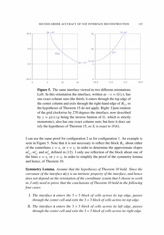
SECOND-ORDER ACCURACY OF VOF INTERFACE RECONSTRUCTION 119
−3h/2
−h/2
h/2
3h/2
0 h 2h 3h
G(y)
(yl,−xl)
(yr,−xr)
−3h/2 −h/2 h/2 3h/20
h
2h
3h
g(x)
(xl, yl)
(xr, yr)
Figure 5. The same interface viewed in two different orientations.Left: In this orientation the interface, written as −x = G(y), hasone exact column sum (the third); it enters through the top edge ofthe center column and exits through the right-hand edge of Bi j , sothe hypotheses of Theorem 15 do not apply. Right: Upon rotationof the grid clockwise by 270 degrees the interface, now describedby y = g(x) (g being the inverse funtion of G, which is strictlymonotonic), also has one exact column sum; but here it does sat-isfy the hypotheses of Theorem 15, so Si is exact to O(h).
I can use the same proof for configuration 2 as for configuration 1. An example isseen in Figure 5. Note that it is not necessary to reflect the block Bi j about eitherof the centerlines x = xc or y = yc in order to determine the approximate slopesml
i j , mci j and mr
i j defined in (12). I only use reflection of the block about one ofthe lines x = xc or y = yc in order to simplify the proof of the symmetry lemmaand hence, of Theorem 10.
Symmetry Lemma. Assume that the hypotheses of Theorem 10 hold. Since thecurvature of the interface z(s) is an intrinsic property of the interface, and hencedoes not depend on the orientation of the coordinate system that I choose to workin, I only need to prove that the conclusions of Theorem 10 hold in the followingfour cases:
I. The interface z enters the 3 × 3 block of cells across its top edge, passesthrough the center cell and exits the 3× 3 block of cells across its top edge.
II. The interface z enters the 3 × 3 block of cells across its left edge, passesthrough the center cell and exits the 3× 3 block of cells across its right edge.

120 ELBRIDGE GERRY PUCKETT
III. The interface z enters the 3 × 3 block of cells across its top edge, passesthrough the center cell and exits the 3× 3 block of cells across its bottomedge.
IV. The interface z enters the 3× 3 block of cells across its left hand edge, passesthrough the center cell and exits the 3× 3 block of cells across its top edge.
Proof. As already noted, without loss of generality I may assume that the arc lengths has been chosen so that the interface is traversed from left to right as s increases.In particular, this implies that I do not need to consider any case in which theinterface enters the 3× 3 block of cells across its right edge.
To assist the reader in following the argument that I need only consider casesI–IV, the following is a list of all of the ways in which the interface g can enterand exit the 3× 3 block of cells together with which of cases I–IV it is equivalentto.
(1) The interface z enters the 3× 3 block of cells across the left edge and exitsacross:(a) The left edge. This violates the assumption that the cell size h is suffi-
ciently small that the interface can be written as a function of one of thecoordinate variables in terms of the other in the 3× 3 block of cells Bi j .
(b) The right edge. This is case II. Since, the interface can be written as afunction on the 3× 3 block of cells Bi j and the first time that the interfaceexits Bi j is across the right-hand edge, it has three exact column sums asshown, for example, in Figure 1. Thus, I have just proved that Theorem10 holds for case II.
(c) The top edge. This is case IV in the statement of the Symmetry Lemmaand is the subject of Lemma 13 and Theorem 15 below. (All of the work inSection 3.2 below is concerned with proving this case when the interfaceis an increasing, monotonic function of x .)
(d) The bottom edge. After reflection about the line y = yc and reversal of thearc length parameter s→ s ′ =−s this is equivalent to (1c) immediatelyabove and hence falls under case IV in the statement of the SymmetryLemma.
(2) The interface z enters the 3× 3 block of cells across the top edge and exitsacross:(a) The left edge. Upon reversal of the arc length parameter s→ s ′ =−s this
case is equivalent to case (1c), and hence is equivalent to case IV in thestatement of the theorem.
(b) The right edge. Upon reflection of the 3 × 3 block of cells about themidline x = xc this case is equivalent to case (1c), and hence is equivalentto case IV in the statement of the theorem.

SECOND-ORDER ACCURACY OF VOF INTERFACE RECONSTRUCTION 121
(c) The bottom edge. This is case III of the Symmetry Lemma. It has twosubcases:(i) The interface y = g(x) is strictly monotonic in the 3×3 block of cells
Bi j , and therefore it is invertible. Rotating the 3× 3 block of cells90 degrees counterclockwise yields case (1b) and hence this case isequivalent to case II of the Symmetry Lemma. I have already proventhat Theorem 10 holds in this case.
(ii) The interface z is not strictly monotonic in the 3× 3 block of cellsBi j . In Lemma 12 I will prove that this case cannot occur.
(d) The top edge. This is case I of the symmetry lemma. In Lemma 11 I willprove that the condition on the maximum curvature κmax in Equation (3)prevents this case from occurring.
(3) The interface z enters the 3× 3 block of cells Bi j across the bottom edge andexits across:(a) The left edge. After rotation of the block Bi j clockwise by 90 degrees
this case is equivalent to case (1c), and hence is equivalent to case IV ofthe symmetry lemma.
(b) The right edge. After rotation of the block Bi j by 180 degrees and reversalof the arc length parameter s→ s ′ = −s this case is equivalent to case(1c), and hence is equivalent to case IV of the symmetry lemma.
(c) The bottom edge. After rotation of the block Bi j by 180 degrees andreversal of the arc length parameter s→ s ′ =−s this case is equivalent to(2d) which is case I of the symmetry lemma, which I prove cannot occur.
(d) The top edge. After rotation of the block Bi j by 180 degrees and reversalof the arc length parameter s → s ′ = −s this case is equivalent to (2c)above.
(4) The interface z enters the 3× 3 block of cells Bi j across the right-hand edgeand exits across:(a) The right edge. As in case (1a) above, this violates the assumption that
the cell size h is sufficiently small that the interface can be written as afunction in the block Bi j and hence, this case is not allowed.
(b) The left edge.(c) The bottom edge.(d) The top edge.
In each of cases 4(b-d) I can change the parametrization of the interface byinterchanging the arc length parameter s with s ′ =−s so that the interface en-ters the 3×3 block of cells Bi j across its left, bottom, or top edge respectivelyand exits Bi j across its right edge. Therefore, cases 4(b-d) are equivalent tocases 1(b), 3(b), and 2(d), respectively. �

122 ELBRIDGE GERRY PUCKETT
In order to prove that if the interface satisfies the hypotheses of Theorem 10,then it has at least two column sums that are exact to O(h), I will often need toseparate the proof into two parts:
A. The interface g is a strictly monotonic function on the interval under consid-eration.
B. The interface g is not a strictly monotonic function on the interval under con-sideration.
Recall that a function g(x) is strictly monotonic on the interval [a, b] if and onlyif x < y H⇒ g(x) < g(y) for all x, y ∈ [a, b]. In the following, when I refer tothe interface g as being strictly monotonic or not strictly monotonic, the interval[a, b] is implicitly understood to be [x0, x3]; that is, the bottom edge of the 3× 3block of cells Bi j under consideration.
Recall that ξ is called a critical point of the function g if and only if g′(ξ)= 0.If the function g is a strictly monotonic function on [x0, x3], then it cannot have acritical point in [x0, x3]. In the simplest cases, if g is strictly monotonic then, sinceit is invertible, the 3× 3 grid can be rotated by 90 degrees and an interface that hasonly one or no exact column sums in the original orientation will have two or threeexact column sums in the new orientation. However in one case — namely, the oneshown in Figure 5 — the lack of a critical point makes it much more difficult toprove that the interface has at least two column sums that are exact to O(h). Theexistence of a critical point ξ ∈ [x0, x3] greatly simplifies the proof of Lemmas 11–13. In fact, as will become apparent from the proofs of these lemmas, the existenceof a critical point ξ ∈ [x0, x3] is sufficient to force the middle column sum Si to beexact.
Lemma 11 (Case I of the Symmetry Lemma cannot occur). Let g ∈ C2[x0, x3] be
a nonmonotonic function that satisfies the assumptions of Theorem 10. Then caseI of the symmetry lemma cannot occur; the interface cannot enter the 3× 3 blockof cells Bi j across its top edge at some point (xl, y3), pass through the center cellCi j of Bi j , and exit Bi j across its top edge at some point (xr , y3).
Proof. Since g is assumed to cross the line y = y3 twice in the interval [x0, x3] it isnot monotonic, and since g must pass through the center cell of the 3× 3 block, itfollows that g must have at least one critical point ξ ∈ [x0, x3] such that g′(ξ)= 0and y3− g(ξ) > h. There are two cases:
A. x3− ξ ≤ 3h/2; that is, ξ lies to the right of the midline x = xc of the blockBi j .
B. x3− ξ > 3h/2; that is, ξ lies to the left of the midline x = xc of the block Bi j .
I will prove the theorem for case A. I will then indicate the changes one needsto make in the proof of case A in order to prove case B. Consider the parabolic

SECOND-ORDER ACCURACY OF VOF INTERFACE RECONSTRUCTION 123
comparison function p defined by
p(x)= a(x − ξ)2+ g(ξ),
where the coefficient a is given by
a =y3− g(ξ)(x − ξ)2
(55)
and x = x3+ h/4. See Figure 6 for an example. Note that a was chosen so that
p(x)= g(xr )= y3, p′(ξ)= g′(ξ)= 0. (56)
Since g(xr )= y3 and p is a monotone increasing function for x >ξ , and ξ < xr < x ,I must have g(xr ) > p(xr ). Thus, the difference f (x) = g(x)− p(x) between gand p satisfies
f (ξ)= g(ξ)− p(ξ)=0, f ′(ξ)= g′(ξ)− p′(ξ)=0, f (xr )= g(xr )− p(xr )>0.(57)
x0 x1 x2 x3 x4xc
|y0
y1
y2
y3
+(ξ, g(ξ)))
ξ
|
•(xr, yr)•(xl, yl)
g(x)
x
|
•(x, y3)
p(x)
Figure 6. An example in which the interface g(x) enters the topedge of the 3× 3 block of cells Bi j at the point (xl, yl)= (xl, y3),passes through the center cell Ci j and leaves Bi j at the point(xr , yr )= (xr , y3). The function p(x) is the parabolic comparisonfunction that I use for this particular interface in the proof of caseA of Lemma 11. The presence of a critical point (ξ, g(ξ)) ∈ Bi j
with g(ξ) < y2 is essential to the successful use of a paraboliccomparison function in the proof of Lemma 11.

124 ELBRIDGE GERRY PUCKETT
The first and last of these equations imply there exists ζ ∈ [ξ, xr ] such that
f ′(ζ )= g′(ζ )− p′(ζ ) > 0, (58)
and this, together with the middle equation in (57), imply there exists η ∈ [ξ, ζ ]such that
f ′′(η)= g′′(η)− p′′(η) > 0. (59)
In other words,
g′′(η) > p′′(η)= 2a for some η ∈ [ξ, ζ ]. (60)
Since x3− ξ ≤ 3h/2, it follows that x − ξ ≤ 7h/4, and hence that
1(x − ξ)2
≥16
49h2 .
This inequality, together with y3− g(ξ) > h, imply
g′′(ξ) > 2a = 2(y3− g(ξ))(x − ξ)2
>32h49h2 >
3249h
.
From (47), I havemax
x∈[x0,x3]|g′′(x)| ≤ 8κmax,
and hence κg(ξ)≥ g′′(ξ)/8 where κg(x) denotes the curvature of the interface g(x)at the point (x, g(x)). Thus
κg(ξ)≥g′′(ξ)
8>
449h
>4
52h=
113h
. (61)
Since Ch =
√2−1
4√
3<
116
, it follows from (61) that
κgmax ≥ κ
g(ξ) >1
13h>
Ch
h.
Hence, the interface does not satisfy the assumption (3) and thus this interfaceconfiguration cannot occur.
In the event that case B holds, replace (xr , y3) with (xl, y3), set x = x0−h/4, etc.,and the proof that case I of the symmetry lemma cannot occur when x3− ξ > 3h/2(case B) is essentially identical to the proof when x3− ξ ≤ 3h/2 (case A). �
Recall that in the proof of the Symmetry Lemma, I showed that case II willalways have three exact column sums. Hence case II has already been proved.Therefore, I must now consider case III of the Symmetry Lemma. In the proof ofthat case, I showed that when the interface function g is strictly monotonic it isequivalent to case II of the Symmetry Lemma, so it also has three exact columnsums. Therefore, I only need to consider the nonmonotonic version of case III.

SECOND-ORDER ACCURACY OF VOF INTERFACE RECONSTRUCTION 125
Lemma 12 (Nonmonotonic version of case III of the Symmetry Lemma). Let g ∈C2[x0, x3] be a nonmonotonic function satisfying the assumptions of Theorem 10.
Then case III of the Symmetry Lemma cannot occur; that is, the interface cannotenter the 3× 3 block of cells Bi j across its top edge at some point (xl, y3), passthrough the center cell Ci j of Bi j , and exit Bi j across its bottom edge at some point(xr , y0) with x0 ≤ xl < xr ≤ x3.
Proof. I will show that if the interface g enters the 3×3 block of cells Bi j across itstop edge, passes through the center cell Ci j of Bi j , and exits Bi j across its bottomedge, then it cannot satisfy
κgmax ≤ Chh−1 (62)
and hence it fails to satisfy the first constraint in (3).First note that since g is nonmonotonic there is at least one point ξ ∈ [x0, x3]
such that g′(ξ) = 0. As in the proof of Lemma 11 there are two cases: A and B.However, in this proof I must also consider two subcases of each of these cases:
A. The points ξ and x3 satisfy x3 − ξ ≤ 3h/2 and one of the following twoconditions hold:
(i) y3− g(ξ) > h (ii) y3− g(ξ)≤ h
B. The points ξ and x3 satisfy x3 − ξ > 3h/2 and one of the following twoconditions hold:
(i) y3− g(ξ) > h (ii) y3− g(ξ)≤ h
I will prove the lemma for case B(i). The proofs of the other three cases are nearlyidentical.
Therefore, assume that x3− ξ > 3h/2 and y3− g(ξ) > h both hold and considerthe parabolic comparison function
p(x)= a(x − ξ)2+ g(ξ)
where the coefficient a is defined by
a =3h− g(ξ)(x − ξ)2
(63)
and x is defined by x = x0− h/4. Note that a was chosen so that
p(x)= y3 = 3h, p′(ξ)= g′(ξ)= 0. (64)
Since x < xl < ξ and p is a monotone decreasing function for x < ξ , I must haveg(xl) > p(xl) as shown in Figure 7. Thus, the difference f (x) = g(x)− p(x)between g and p satisfies
f (ξ)=g(ξ)− p(ξ)=0, f ′(ξ)=g′(ξ)− p′(ξ)=0, f (xl)=g(xl)− p(xl)>0.(65)

126 ELBRIDGE GERRY PUCKETT
x−1 x0 x1 x2 x3
y0
y1
y2
y3
ξ|
g(ξ)−x|
g(x)p(x)
(xl, yl)
(xr, yr)
Figure 7. An example in which the interface g(x) enters the3× 3 block of cells Bi j at its upper left corner (xl, yl) = (x0, y3).It then passes through the center cell and leaves Bi j at its lowerright corner (xr , yr ) = (x3, y3). The function p is the paraboliccomparison function used in the proof of case B(1) of Lemma 12.
The first and last of these equations imply that there exists ζ ∈ [xl, ξ ] such that
f ′(ζ )= g′(ζ )− p′(ζ ) < 0, (66)
and this, together with the middle equation in (65), implies there exists η ∈ [ζ, ξ ]such that
f ′′(η)= g′′(η)− p′′(η) > 0. (67)
In other words,
g′′(η) > p′′(η)= 2a for some η ∈ [ζ, ξ ]. (68)
Note that ξ − x0 ≤ 3h/2 implies that ξ − x ≤ 7h/4. This inequality, together withy3− g(ξ) > h, implies
g′′(η) > p′′(η)= 2a = 2y3− g(ξ)(x − ξ)2
>32h49h2 .
As in the proof of Lemma 11, it follows from (47) that κg(ξ) > g′′(ξ)/8; hence
κg(ξ)≥g′′(ξ)
8>
449h
>4
52h>
113h
. (69)

SECOND-ORDER ACCURACY OF VOF INTERFACE RECONSTRUCTION 127
Consequently,
κgmax ≥ κ
g(ξ) >1
13h>
Ch
h,
whereby g fails to satisfy (62), and hence the constraint in (3) as claimed. �
Lemma 13 (Case IV of the Symmetry Lemma). Let g ∈ C2[x0, x3] be a function
that satisfies the assumptions of Theorem 10. Assume also that the interface genters the 3× 3 block of cells Bi j across its left edge at the point (xl, yl)= (x0, yl),passes through the center cell Ci j = [x1, x2]× [y1, y2], and exits Bi j across its topedge at (xr , yr ) = (xr , y3) with x1 < xr ≤ x3. Then the interface has at least twocolumn sums in Bi j that are either exact or exact to O(h).
Proof. I will proceed by dividing the problem into two major divisions: (1) thecase in which the interface is strictly monotonic and (2) the case in which it isnot. The examples in which the center column sum is not exact in any of the fourstandard orientations of the block Bi j — as shown, for example, in Figures 3, 5, 9and 10 — are in the strictly monotonic category of case IV; the first of these twomajor divisions.
In order to make the argument as clear as possible, I have enumerated the proofof case IV into its various subdivisions here.
(1) The interface g is strictly monotonically increasing.(a) The ordinate yl of the point (x0, yl) satisfies y0≤ yl ≤ y1. Since g is strictly
monotonic, it is invertible. Therefore it can be written as a function x =g−1(x) on the interval [y0, y3]. Furthermore, since it must pass throughthe center cell Ci j = [x1, x2]× [y1, y2] before exiting the block Bi j acrossits top edge, rotation of the block clockwise by 90 degrees will yield anorientation in which the second and third column sums are exact. Thus,this particular case of the lemma is proved.
(b) The ordinate yl of the point (x0, yl) satisfies y1 < yl < y2. There are twosubdivisions of this case:(i) The abscissa xr of the point (xr , y3) at which the interface exits Bi j
satisfies x2 ≤ xr ≤ x3. In this case the column sums Si−1 and Si areboth exact and the lemma is again proved.
(ii) The abscissa xr of the point (xr , y3) at which the interface exits Bi j isstrictly less than right-hand edge x = x2 of the second column. Sincethe interface is assumed to be a function y = g(x) on the interval[x0, x3], and since it must pass through the center cell Ci j = [x1, x2]×
[y1, y2], I have x1 < xr < x2. In this case the first column sum Si−1 isexact and, since the interface satisfies the constraint κmax ≤ (
√h)−1
in (3), the second column sum Si is exact to O(h). I will prove thislatter statement in Theorem 15 below.

128 ELBRIDGE GERRY PUCKETT
(c) The ordinate yl of the point (x0, yl) at which g enters Bi j satisfies y2 ≤
yl ≤ y3. Since the interface is strictly monotonically increasing, it cannotenter the center cell Ci j = [x1, x2] × [y1, y2] if yl ≥ y2. This contradictsthe basic assumption that the interface passes through Ci j . Therefore thiscase must be excluded.
(2) The interface is not strictly monotonically increasing.
(a) The abscissa xr of the point (xr , y3) at which the interface exits the blocksatisfies x2 ≤ xr ≤ x3. In this case the column sums Si−1 and Si are exactand once again the lemma is proved.
(b) The abscissa xr of the point (xr , y3) at which the interface g exits Bi j isless than right-hand edge of the second column; that is, xr < x2. In thiscase, since g is not strictly monotonic, and since it must pass through thecenter cell Ci j = [x1, x2]× [y1, y2], g must have a critical point (ξ, g(ξ))with y3 − g(ξ) > h which is also a local minimum of g. An exampleappears in Figure 8. I will now prove that this is inconsistent with
κgmax ≤
Ch
h, (70)
and hence with the constraint in (3).
Proof of case (2b). Assume that the conditions listed in (2b) above hold and recallthat the point (ξ, g(ξ)) is a local minimum of g. I form a comparison function pof the form
p(x)= a(x − ξ)2+ g(ξ), (71)
where the coefficient a is defined by
a =y3− g(ξ)(ξ − x2)2
. (72)
Note that a was chosen so that
p(x2)= y3 = 3h, p′(ξ)= g′(ξ). (73)
Since p is a monotone increasing function for ξ < x and ξ < xr I must haveg(xr ) > p(xr ) as shown, for example, in Figure 8.
Thus, the difference f (x)= g(x)− p(x) between g and p satisfies
f (ξ)= g(ξ)− p(ξ)=0, f ′(ξ)= g′(ξ)− p′(ξ)=0, f (xr )= g(xr )− p(xr )>0.(74)
The first and last of these equations imply there exists ζ ∈ [ξ, xr ] such that
f ′(ζ )= g′(ζ )− p′(ζ ) > 0, (75)
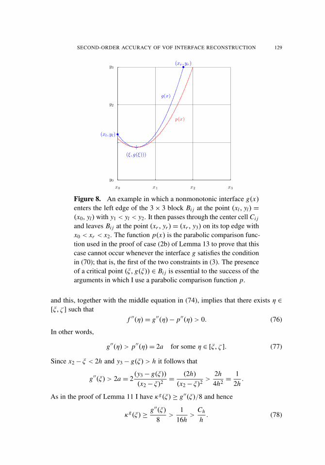
SECOND-ORDER ACCURACY OF VOF INTERFACE RECONSTRUCTION 129
x0 x1 x2 x3
y0
y2
y3
+(ξ, g(ξ)))
•(xr, yr)
•(xl, yl)
g(x)
p(x)
Figure 8. An example in which a nonmonotonic interface g(x)enters the left edge of the 3× 3 block Bi j at the point (xl, yl) =
(x0, yl) with y1 < yl < y2. It then passes through the center cell Ci j
and leaves Bi j at the point (xr , yr )= (xr , y3) on its top edge withx0 < xr < x2. The function p(x) is the parabolic comparison func-tion used in the proof of case (2b) of Lemma 13 to prove that thiscase cannot occur whenever the interface g satisfies the conditionin (70); that is, the first of the two constraints in (3). The presenceof a critical point (ξ, g(ξ)) ∈ Bi j is essential to the success of thearguments in which I use a parabolic comparison function p.
and this, together with the middle equation in (74), implies that there exists η ∈[ξ, ζ ] such that
f ′′(η)= g′′(η)− p′′(η) > 0. (76)
In other words,
g′′(η) > p′′(η)= 2a for some η ∈ [ξ, ζ ]. (77)
Since x2− ξ < 2h and y3− g(ξ) > h it follows that
g′′(ξ) > 2a = 2(y3− g(ξ))(x2− ξ)2
=(2h)
(x2− ξ)2>
2h4h2 =
12h.
As in the proof of Lemma 11 I have κg(ξ)≥ g′′(ξ)/8 and hence
κg(ξ)≥g′′(ξ)
8>
116h
>Ch
h. (78)

130 ELBRIDGE GERRY PUCKETT
Consequently, κgmax ≥ κ
g(ξ) > Ch/h, whereby g fails to satisfy (70) and hence, theconstraint on κmax in (3) as claimed. �
3.2. The comparison circle z(s). All that remains is to prove (ii) from case (1b)in the preceding proof. This is the case in which the center column sum is not exactin each of the four standard orientations of the block Bi j as shown in the examplesin Figures 3 and 5. The remainder of this section is devoted to proving this result,which is stated explicitly in Theorem 15 below.
Notation. In what follows it will be convenient to translate the coordinate systemso that the origin coincides with the point (x0, y1). This results in the follow-ing relations, which I will use in several of the proofs below: (x0, y1) = (0, 0),(x1, y2)= (h, h), and (x2, y3)= (2h, 2h), where x0, . . . , x3 and y0, . . . , y3 are thecoordinates of the grid lines as shown, for example, in Figure 9.
x0 = 0 x1 = h x2 = 2h x3 = 3h
y0 = −h
y1 = 0
y2 = h
y3 = 2h
•(xl, yl)
•(xr, yr)
g(x)
•(xr , yr)
c(x) = z(s)
×(x0, y0)
Figure 9. In this figure g is an arbitrary strictly monotonicallyincreasing function that enters the 3× 3 block Bi j through its leftedge at the point (xl, yl) with y1 ≤ yl < y2, passes through thecenter cell Ci j , and exits Bi j through the top of its center columnSi at the point (xr , yr ) with x1 < xr < x2. Lemma 16 says that if gsatisfies κmax ≤ (
√h)−1, the distance x2− xr is O(h3/2). In order
to prove this, I form a comparison function z(s) which is a circlethat has curvature κ = (
√h)−1 and passes through (x0, y1) and
(x1, y2). In the circle comparison theorem (Theorem 14) I provethat g must eventually lie below the graph of z, thereby implyingthat xr < xr . Then, in Lemma 17, I prove that x2− xr is O(h3/2).

SECOND-ORDER ACCURACY OF VOF INTERFACE RECONSTRUCTION 131
Now consider the circle z(s)= (x(s), x(s)) defined by
x(s)= R sin(φ0+
sR
)− R sinφ0, y(s)=−R cos
(φ0+
sR
)+ R cosφ0, (79)
together with the parameters
φ0 =π4− sin−1 R
√2=π4−
s12R, (80)
s1 = 2R sin−1 R√
2, s2 = R cos−1(cosφ0− 2R)− Rφ0. (81)
It is relatively straightforward to check the equalities
z(0)=(x0,y1)=(0,0), z(s1)=(x1,y2)=(h,h), z(s2)=(xr ,y3)=(xr ,2h). (82)
Note that the variable xr in the last of these equations plays the same role withrespect to the function z(s) as the variable xr plays with respect to the interfacez(s)= (x, g(x)). Namely, xr is the x-coordinate at which the graph of z(s) exitsthe top of the 3× 3 block Bi j . This is illustrated in Figure 9. In what follows I willoften use (x, c(x)) to denote the graph of z(s) reparametrized as a function of xjust as I use (x, g(x)) to denote the graph of the interface z(s).
3.3. The circle comparison theorem. Suppose that the interface (x, g(x)) satisfiesκmax ≤ (
√h)−1. In the following theorem I prove that once g(x) < c(x) for some
x ∈ (x0, x2), then g(x) must remain below c(x) for all x ∈ (x0, xr ), where (x0, y0)
is the point at which g initially crosses c as shown in Figure 9. An immediateconsequence of this fact is that xr ≤ xr . Consequently, if xr < x2, then xr ≤ xr < x2
and hence |x2− xr | ≤ |x2− xr |. Since I have constructed the comparison functionc so that I can easily show that |x2 − xr | is O(h3/2), it follows that |x2 − xr | isO(h3/2). This, together with the fact that g′(x) ≤
√3 from (46), is sufficient to
show that the error in the second column sum associated with g is O(h).
Theorem 14 (The circle comparison theorem). Assume that R =√
h and let g ∈C2[x0, x3] be a strictly monotonic function that satisfies
κmax ≤ (√
h)−1. (83)
Furthermore, assume that g enters the 3× 3 block of cells Bi j on its left edge at thepoint (xl, yl) with y1 < yl < y2, passes through the center cell Ci j , and exits Bi j
through the top of its center column at the point (xr , yr )= (xr , y3) with x1< xr < x2.Let (x0, y0) denote the first point at which the graph of g crosses the graph of c asshown in, for example, Figure 9. Then
g(x) < c(x) for all x ∈ (x0, xr ]. (84)

132 ELBRIDGE GERRY PUCKETT
Proof. First note that since c is a circle, the curvature of c is constant: κ c= (√
h)−1.Hence, by (83),
κg(x)≤ κ c(x) for all x ∈ [x0, xr ].
To prove that (84) is true I start by assuming that
g(ξ)= c(ξ) for some ξ ∈ (x0, xr ], (85)
and then show that this implies that the maximum curvature κmax of g in (x0, xr )
must exceed (√
h)−1, thereby contradicting (83).Since g(x) > c(x) for x0 < x < x0 and g(x) < c(x) for x0 < x < ξ it follows
thatg′(x0) < c′(x0). (86)
However, since by (85) g(ξ) = c(ξ) for some ξ > x0 it must be the case thateventually g′(x)≥ c′(x). Therefore let x∗ ∈ (x0, ξ) be the first x such that g′(x∗)=c′(x∗). I have
g′(x∗)= g′(x0)+
∫ x∗
x0
g′′(x) dx = c′(x0)+
∫ x∗
x0
c′′(x) dx = c′(x∗),
which, by virtue of (86), can only be true if g′′(x) > c′′(x) on some subinterval of(x0, x∗). So in particular g′′(η) > c′′(η) for some η ∈ (x0, x∗). Now recall that
(1) g is strictly monotonic and hence 0< g′(x) for all x ∈ (x0, xr ].
(2) 0< g′(x) < c′(x) for all x ∈ (x0, x∗).
(3) κg(x)= g′′(x)(1+ g′(x)2)−3/2 for all x .
Items (1)–(3) imply that
κg(η)=g′′(η)
(√
1+ g′(η)2)3>
c′′(η)
(√
1+ c′(η)2)3= κ c(η)=
1√
h,
which contradicts (83) as claimed. �
3.4. The column sum Si is exact to O(h).
Theorem 15 (The column sum Si is exact to O(h)). Assume that the interface g ∈C2[x0, x3] and that g is a strictly monotonically increasing function that satisfies
κmax ≤ (√
h)−1. (87)
Furthermore, assume that the g enters the 3× 3 block of cells Bi j on its left edgeat the point (xl, yl) with y1 ≤ yl ≤ y3, passes through the center cell Ci, j =
[x1, x2] × [y1, y2], and exits Bi j through the top of its center column at the point(xr , yr )= (xr , y3) with x1 < xr < x2 as shown, for example, in Figure 10. Then the

SECOND-ORDER ACCURACY OF VOF INTERFACE RECONSTRUCTION 133
x0 x1 x2 x3
y0
y1
y2
y3
y4
•(xl, yl)
• (xr, yr)
g(x)
c(x) = z(s)
×(x0, y0)
Figure 10. To see the error between the center column sum Si
and the exact volume (area) under the interface y = g(x), I haveplotted the row of cells that lie above the standard 3× 3 block ofcells Bi, j centered on the cell Ci, j = [x1, x2] × [y1, y2] in whichthe approximation to the interface g will be constructed. I havealso plotted the comparison circle c(x) which, in Theorem 14, Iprove provides an upper bound on g(x) for all x ∈ [x0, x2] where(x0, y0) is the point at which the interface g intersects comparisoncircle c.
error between the column sum Si and the normalized integral of g over the secondcolumn is O(h): ∣∣∣Si − h−2
∫ x2
x1
(g(x)− y0)dx∣∣∣≤ CSh, (88)
whereCS = 8
√3(2√
2− 1)2. (89)
Proof. As one can see from the example shown in Figure 10, the error betweenthe column sum Si and the exact normalized volume (area) under the interfacey = g(x) in the center column is
h−2∫ x2
x1
(g(x)− y0)dx − Si = h−2∫ x2
xr
(g(x)− y3)dx,
since
Si = h−2∫ x2
x1
(min{g(x), y3}− y0)dx,

134 ELBRIDGE GERRY PUCKETT
and, by assumption, min[x0,xr ]
g(x)≥ yl ≥ y1. Thus, it suffices to show that∣∣∣∣∫ x2
xr
(g(x)− y3)dx∣∣∣∣≤ CSh3. (90)
In other words, I need to show that the volume in the region below the interfacey = g(x) that lies in the cell C2,4 is O(h3).
By (46) in I have |g′(x)| ≤√
3. This implies∣∣∣∣∫ x2
xr
(g(x)− y3)dx∣∣∣∣≤ ∣∣∣∣∫ x2
xr
l(x)dx∣∣∣∣, (91)
where l(x) is the line with slope√
3 that passes through the point xr . The regionof integration on the right side of (91) is a right triangle with corners (xr , y3),(x2, y3), and (x2, y3 +
√3(x2 − xr )) and the integral is the area of this triangle,
namely,√
3(x2− xr )2/2. Thus I have∣∣∣∣∫ x2
xr
(g(x)− y3) dx∣∣∣∣≤ ∣∣∣∣∫ x2
xr
l(x) dx∣∣∣∣≤√
32(x2− xr )
2≤
√3
2C2h3, (92)
where the bound (x2−xr )2≤ C2h3 between the second to last and last terms in (92)
follows from the inequality (93) immediately below. Equation (92) implies (90).Equation (88) — and hence the theorem — follows immediately. �
Lemma 16 (x2− xr is O(h3/2)). Let g ∈ C2[x0, x3] be a function that satisfies the
assumptions stated in Theorem 14. Then
x2− xr ≤ Ch3/2, (93)
whereC = 4(2
√2− 1). (94)
Proof. By the circle comparison theorem (Theorem 14) there exists a point x0 ∈
[x0, xr ) such thatg(x)≤ c(x) for all x ∈ [x0, xr ].
This implies that xr ≤ xr . Since by assumption xr < x2, Equation (93) followsimmediately from Equation (95) in Lemma 17 below. �
Lemma 17 ( x2 − xr is O(h3/2)). Let R =√
h and let xr be defined as in (82)above. Then
x2− xr ≤ Ch3/2, (95)
where C is defined in (94).
Proof. Since the coordinate system has been arranged so that the origin is at thepoint (x0, y1) and hence x2 = 2h = y3 (for example, see Figure 9), I have
x2 = yr = y(s2).
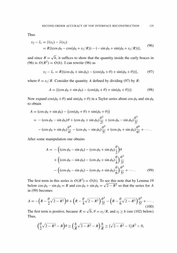
SECOND-ORDER ACCURACY OF VOF INTERFACE RECONSTRUCTION 135
Thus
x2− xr = y(s2)− x(s2)
= R{(cosφ0− cos(φ0+ s2/R))− (− sinφ0+ sin(φ0+ s2/R))},(96)
and since R =√
h, it suffices to show that the quantity inside the curly braces in(96) is O(R2)= O(h). I can rewrite (96) as
x2− xr = R{(cosφ0+ sinφ0)− (cos(φ0+ θ)+ sin(φ0+ θ))}, (97)
where θ = s2/R. Consider the quantity A defined by dividing (97) by R:
A = {(cosφ0+ sinφ0)− (cos(φ0+ θ)+ sin(φ0+ θ))}. (98)
Now expand cos(φ0+ θ) and sin(φ0+ θ) in a Taylor series about cosφ0 and sinφ0
to obtain
A = (cosφ0+ sinφ0)−(cos(φ0+ θ)+ sin(φ0+ θ)
)= − (cosφ0− sinφ0)θ + (cosφ0+ sinφ0)
θ2
2!+ (cosφ0− sinφ0)
θ3
3!
− (cosφ0+ sinφ0)θ4
4!− (cosφ0− sinφ0)
θ5
5!+ (cosφ0+ sinφ0)
θ6
6!+ · · · .
After some manipulation one obtains
A = −((cosφ0− sinφ0)− (cosφ0+ sinφ0)
θ
2
)θ
+
((cosφ0− sinφ0)− (cosφ0+ sinφ0)
θ
4
)θ3
3!
−
((cosφ0− sinφ0)− (cosφ0+ sinφ0)
θ
6
)θ5
5!+ · · · . (99)
The first term in this series is O(R2)= O(h). To see this note that by Lemma 19below cosφ0− sinφ0 = R and cosφ0+ sinφ0 =
√2− R2 so that the series for A
in (99) becomes
A =−(
R− θ2
√2− R2
)θ +
(R− θ
4
√2− R2
)θ3
3!−
(R− θ
6
√2− R2
)θ5
5!+ · · · .
(100)The first term is positive, because R =
√h, θ = s2/R, and s2 ≥ h (see (102) below).
Thus, (θ2
√2− R2− R
)θ ≥
( hR
√2− R2− R
) hR≥(√
2− R2− 1)R2 > 0,

136 ELBRIDGE GERRY PUCKETT
for all 0< h ≤ 1, and hence all 0< R ≤ 1. Similarly, since s2 ≤ 4h (see Lemma18 again), it follows that(
θ2
√2− R2− R
)θ ≤
(2R√
2− R2− R)4R = 4
(2√
2− R2− 1)R2, (101)
for all 0< h ≤ 1, or equivalently all 0< R ≤ 1. Combining equations (97), (98),(100), and (101) yields
x2− xr ≤ 4(2√
2− R2− 1)R3+ O(R5)≤ 4(2
√2− 1)R3
+ O(R5).
It is possible to show — for example by plotting it with MATLAB — that the co-efficient (R− θ
√2− R2)/4 of the second term in the expansion of A in terms of
R in (100) is negative for 0< h ≤ 1 and that furthermore, the tail of the series isbounded by this term. Equation (95) follows immediately. �
Lemma 18 (s2 = O(h)). Assume that h ≤ 1 and let s2 be defined as in (81). Then
h ≤ s2 ≤ 4h. (102)
Proof. First, note that I am only interested in functions g that exit the 3× 3 blockof cells at the point (xr , y3) when xr < x2 as shown for example in Figure 3. Forotherwise the first and second column sums would be exact and I would be done.
x0 x1 x2 x3
y0
y1
y2
y3
•(x(0), y(0))
•(x(s2), y(s2)) = (xr, yr)
z(s)
Figure 11. In this figure h = 14 and hence the comparison circle
z(s) has radius R =√
h = 2h.

SECOND-ORDER ACCURACY OF VOF INTERFACE RECONSTRUCTION 137
Since a consequence of Theorem 14 is that xr = x(s2) ≤ xr , it follows that I amonly interested in values of R =
√h and s2 such that xr < x2.
To obtain the lower bound on s2 in (102) note that s2 is an arc of the circlez and that when h = 1 the radius of z is R =
√h = h. In this case the point
(xr , yr ) = (x0, y3) and hence xr = x0. Since this is half the circumference of thecircle with center (x0, y2) and radius h, s2= π when h = 1. Since s2 will always begreater than the length of the chord connecting the points (x0, y1) and (xr , yr ) andsince this particular chord is the diameter of z all other chords of z will be smaller.In particular, since the radius of z R =
√h→ 0 as h→ 0, all chords connecting
(x0, y1) and (xr , yr ) will be smaller than this one. The lower bound on s2 in (102)follows immediately.
In order to write s2 in the form s2 = Ch where C is a constant independentof h note that since h ≤ 1 and x(s2) < x2, the arc of the circle that connects thepoints (x(0), y(0)) and (x(s2), y(s2)) always lies entirely within the triangle withvertices (x0, y1), (x2, y1) and (x2, y3), as shown in Figure 11, for example. Hence,the arc length s2 will always be bounded above by the sum of the lengths of thetwo perpendicular sides of this right triangle; namely,
s2 < 4h.
This is the upper bound on s2 in (102). �
In order to prove that x2 − xr = O(h3/2) in Lemma 17, I expanded x2 − xr
in a Taylor series about the point φ0. As we saw in Lemma 17 the coefficient ofthe first nonzero term in this expansion is cosφ0 − sinφ0. Hence, the fact thatcosφ0 − sinφ0 = R is a crucial part of the proof that |x2 − xr | = O(h3/2). Thepurpose of the following lemma is to prove this fact and also to establish the valueof cosφ0+ sinφ0.
Lemma 19 (cosφ0− sinφ0 = R). Let φ0 be defined as in (80):
φ0 =π
4− sin−1 R
√2.
Thencosφ0− sinφ0 = R, cosφ0+ sinφ0 =
√2− R2. (103)
Proof. Define θ by sin θ = R/√
2, so that
φ0 =π
4− sin−1 R
√2=π
4− θ.
The first equation in (103) follows from writing φ0 as π/4− θ and applying thetrigonometric identities for the sine and cosine of the difference of two angles:
cosφ0− sinφ0 =√
2 sin θ = R.

138 ELBRIDGE GERRY PUCKETT
To prove the second equality in (103) I again use the trigonometric identities forthe sine and cosine of the difference of two angles, together with the trigonometricidentity cos(arcsin x)=
√1− x2, to obtain
cosφ0+ sinφ0 =√
2 cos θ =√
2 cos(
sin−1 R√
2
)=
√2− R2. �
4. Second-order accuracy in the max norm
In this section I will assume the coordinate system has been arranged so that thebottom edge of the 3× 3 block of cells Bi j lies along the line y = 0 and that thevertical line x = xc which passes through the center of the center cell is x = 0 asshown in Figure 12. In particular, note that the origin is at the center of the bottomedge of the 3× 3 block and the center of Ci j is (0, 3h/2) as shown in the figure.
I will also denote the interval that forms the bottom of the 3× 3 block Bi j by I ,and the intervals [xi−2, xi−1], [xi−1, xi ] and [xi , xi+1] that are associated with thethree columns of Bi j by Ii+α for α =−1, 0, 1. Thus, I = [−3h/2, 3h/2] and
Ii+α ≡
[−3h/2,−h/2] if α =−1,
[−h/2, h/2] if α = 0,
[h/2, 3h/2] if α = 1.
−3h/2 −h/2 h/2 3h/20
h
2h
3h
|(0,0)
+(0,3h/2)
g(x)
Figure 12. In this section I will work with the coordinate systemshown here. The origin is at the center of the bottom of the 3× 3block Bi j so that the center of the center cell Ci j is (0, 3h/2) asshown in the figure. This latter point corresponds to the pointlabeled (xc, yc) in some of the other figures.

SECOND-ORDER ACCURACY OF VOF INTERFACE RECONSTRUCTION 139
Given an arbitrary integrable function g(x) on the interval I = [−3h/2, 3h/2],let 3i, j (g) denote the volume fraction due to g in the center cell
3i, j (g)= h−2∫
Ii
θ j (g(x))dx . (104)
where θ j (g) is defined by
θ j (g)≡ (g(x)− ( j − 1)h)+− (g(x)− jh)+ (105)
and
x+ ={
x if x > 0,0 if x ≤ 0,
(106)
is the ramp function. I will denote the volume fractions in the other cells similarly;that is, I will use 3i ′, j ′(g) for i ′ = i − 1, i, i + 1 and j ′ = j − 1, j, j + 1 to denotethe volume fraction in the (i ′, j ′)-th cell. When the function g under considerationis apparent, I will simply write 3i ′, j ′ or equivalently 3i+α, j+β for some α, β =−1, 0, 1.
In the following lemma I make the implicit assumption that the 3× 3 block ofcells Bi j has been arranged so that the volume fraction 3i, j (g) is the volume (area)of dark fluid in the center cell. In other words, if one assumes that the block Bi j
has been rotated so that the interface z can be represented as a function g(x) onthe interval I = [−3h/2, 3h/2], then there are two possibilities:
(1) 3i, j (g)= h−2∫
Iiθ j (g)dx is the volume of dark fluid in Ci j ,
(2) 3i, j (g)= h−2∫
Iiθ j (g)dx is the volume of light fluid in Ci j .
In the event that (2) holds, one can reflect the 3× 3 block Bi j about the line y = yc,where yc = (y j + y j+1)/2 is the line that divides the block Bi, j in half horizontally,to ensure that case (1) holds. This is necessary because when I write the piecewiselinear approximation gi, j (x)=mi, j x+bi, j to g(x) in Ci, j I am implicitly assumingthat
3i, j (gi, j )= h−2∫
Ii
θ j (gi, j (x))dx
is the volume of dark fluid in Ci, j . It is necessary to be consistent about which fluidis represented by the volume fraction 3i, j in order to prove the following lemma.
Lemma 20 (Equal volume fractions ensure that g intersects g in the center cellCi, j ). Let g(x) be a continuous function on the interval Ii ≡ [−h/2, h/2] andassume that a portion of the interface g(x) passes through the center cell
Ci, j = [−h/2, h/2]× [h, 2h].

140 ELBRIDGE GERRY PUCKETT
Furthermore, assume that the 3× 3 block of cells Bi j centered on Ci, j has beenarranged so that
3i, j (g)= h−2∫
Ii
θ j (g(x))dx (107)
is the (nonzero) volume fraction of dark fluid in Ci, j . Let
g(x)= mx + b (108)
be a piecewise linear approximation to g that passes through the center cell Ci, j
and assume that g and g have the same volume fraction
0<3i, j (g)=3i, j (g) < 1
in Ci j . Then there exists a point x∗ ∈ Ii = [−h/2, h/2] such that
g(x∗)= g(x∗).
Proof. Consider
h−2∫
Ii
[θ j (g(x))− θ j (g(x))
]dx =3i, j (g)−3i, j (g)= 0,
and note that θ j (g) defined in (105) is a strictly monotonically increasing functionof g(x):
g(x) < g(x)⇒ θ j (g(x)) < θ j (g(x)).
Therefore, in order for 3i, j (g)=3i, j (g) to hold, there are two possibilities. Thefirst is that g(x)= g(x) for all x ∈ Ii , in which case the theorem is true and x∗ isany point in Ii .
The second possibility is that there exists a point x− ∈ Ii with g(x−) < g(x−)and there also exists a point x+ ∈ Ii where g(x+) > g(x+). Thus, since bothg(x) and g(x) are continuous, there must be a point x∗ between x− and x+ whereg(x∗)= g(x∗). To see this, consider the function f (x)= g(x)− g(x). The functionf is continuous and furthermore,
f (x+)= g(x+)− g(x+) > 0, f (x−)= g(x−)− g(x−) < 0.
Hence, if x− < x+, then there must exist an x∗ ∈ (x−, x+) ⊂ Ii (or, if x+ < x−,then x∗ ∈ (x+, x−)⊂ Ii ) such that f (x∗)= 0, or equivalently, g(x∗)= g(x∗), asclaimed. �
An immediate consequence of this lemma is that the piecewise constant volume-of-fluid interface reconstruction algorithm as defined below must be first-orderaccurate. The details are as follows.

SECOND-ORDER ACCURACY OF VOF INTERFACE RECONSTRUCTION 141
Definition 21. The piecewise constant VOF interface reconstruction algorithm isdefined by
g(x)= y j−1+ h3i, j (g) for all x ∈ Ii = [xi−1, xi ], (109)
where, as usual, I have assumed that the 3× 3 block Bi j centered about the cell Ci j
in which I want to reconstruct the interface has been rotated so that the interfacecan be written as a single valued function g(x) on the interval I = [−3h/2, 3h/2]and
3i, j (g)= h−2∫
Ii
θ j (g)dx
is the volume of dark fluid in Ci j .
Corollary 22 (The piecewise constant VOF interface reconstruction algorithm isfirst-order). Suppose that the interface passes through a portion of the cell Ci, j
and that it can be represented as a C2 function on the interval I = [−3h/2, 3h/2].Then the piecewise constant interface reconstruction algorithm defined in (109)produces a first-order accurate approximation g to the exact interface g in Ci, j :
|g(x)− g(x)| ≤ CP h for all x ∈ Ii = [−h/2, h/2],
where CP =√
3.
Proof. By assumption the interface g is continuous and passes through the centercell Ci j . Furthermore, the piecewise constant interface reconstruction algorithmdefined in (109) is a member of the class of piecewise linear approximations tog. Therefore, Lemma 20 applies, and hence there exists a point x∗ ∈ Ii such thaty j−1 ≤ g(x∗)≤ y j and
g(x∗)= g(x∗).
The assumption10 that g ∈ C2[I ] allows me to apply Theorem 6 to obtain (see
Equation (46)) ∣∣g′(x)∣∣≤√3 for all x ∈ [−h/2, h/2]. (110)
Thus, applying the Taylor remainder theorem [29] to g(x), I find that for all x ∈[−h/2, h/2]
|g(x)− g(x)| = |g(x∗)+ g′(ξ)(x − x∗)− g(x∗)| ≤ |g′(ξ)h| ≤√
3h,
since ξ = ξ(x) is some number between x and x∗ (that is, ξ ∈ [−h/2, h/2]) andhence, (110) applies. �
10Actually, I only need the interface g to be one times continuously differentiable on Ii ; that is,g ∈ C1
[Ii ]. I have assumed g ∈ C2[I ] here so that I will not have to prove a special version of
Theorem 6 in order to obtain the bound in (46) on g′(x).

142 ELBRIDGE GERRY PUCKETT
Theorem 23 (The approximation to g′ is first-order accurate). Assume that theinterface g ∈ C2
[I ] where I = [−3h/2, 3h/2] and that at least two distinct columnsums Si+α and Si+β with α, β = 1, 0,−1 and α 6= β are exact to O(h):∣∣∣∣Si+α − h−2
∫Ii+α
g(x) dx∣∣∣∣≤ CSh, (111)
∣∣∣∣Si+β − h−2∫
Ii+β
g(x) dx∣∣∣∣≤ CSh, (112)
where
CS = 8√
3(2√
2− 1)2 (113)
is the constant obtained in Theorem 15. Then the slope defined by
m =Si+α − Si+β
α−βfor α, β = 1, 0,−1 with α 6= β
of the piecewise linear approximation g(x) = mx + b to the exact interface gsatisfies
|m− g′(0)| ≤(26
3 κmax+CS)h. (114)
Proof. Note that during the course of proving Theorem 10, I have shown that theonly column sum that may not be exact is the middle one, Si ; for example, see thelist in the proof of the Symmetry Lemma. Therefore, I may assume that
Si+α = h−2∫
Ii+α
g(x)dx if α = 1 or −1. (115)
Now note that the inequality in (88) can be rewritten in the following way. If (88)holds for the i-th column sum Si , then there exists εi > 0 with |εi | ≤ CSh such that
h−2∫
Ii
g(x)dx = Si + εi if α = 0. (116)
In other words, if the column sum Si is not exact, then εi is the area of the regionbounded by the horizontal line y = y3, the vertical line x = x2, and the graph of theinterface y = g(x) as shown in Figure 10. Otherwise, the column sum Si is exactand εi = 0.
By the Taylor remainder theorem
g(x)= g(0)+ g′(0)x + 12 g′′(ξ)x2, (117)

SECOND-ORDER ACCURACY OF VOF INTERFACE RECONSTRUCTION 143
for some ξ ∈ (−x, x).11 Applying (117) to g and performing the integration inequations (115) and (116) for each α =−1, 0, 1 yields
Si−1 = g(0)h−1− g′(0)+ 13
24 g′′(ξ−1)h, (118)
Si = g(0)h−1+
124 g′′(ξ0)h− εi , (119)
Si+1 = g(0)h−1+ g′(0)+ 13
24 g′′(ξ1)h, (120)
where the term with g′(0) has dropped out of the expression for Si , since g′(0)x isan odd function of x and the interval Ii = [−h/2, h/2] is centered about x = 0.
Subtracting the expression in (118) from the expression in (120) and dividingby 2 yields the centered difference approximation to the derivative g′(0) plus errorterms:
Si+1− Si−1
2= g′(0)+ 13
24
(g′′(ξ1)+ g′′(ξ−1)
)h. (121)
Rearranging the terms in (121) and using (47) yields∣∣∣∣ Si+1− Si−1
2− g′(0)
∣∣∣∣= ∣∣ 1324
(g′′(ξ1)+ g′′(ξ−1)
)h∣∣≤ 26
3 κmaxh ≤( 26
3 κmax+CS)h.
Similarly, subtracting Si−1 from Si and Si from Si+1 yield the two one-sided dif-ference approximations to g′(0),
|(Si − Si−1)− g′(0)| ≤( 14
3 κmax+CS)h,
|(Si+1− Si )− g′(0)| ≤( 14
3 κmax+CS)h.
The inequality in (114) follows immediately. �
The following theorem is the main result of this paper.
Theorem 24. Assume the interface g ∈ C2[I ] where I = [−3h/2, 3h/2] and that
at least two of the column sums Si+α and Si+β for α, β = 1, 0,−1 with α 6= β areexact to O(h). Let
g(x)= mx + b
be a piecewise linear approximation to g(x) in Ii = [−h/2, h/2] with
m =Si+α − Si+β
α−β, (122)
and assume that g(x) and g(x) have the same volume fraction in the center cell:
3i, j (g)=3i, j (g).
11Technically speaking, if x > 0, then ξ ∈ (0, x), while if x < 0, then ξ ∈ (x, 0). My intention isfor the notation ξ ∈ (−x, x) to cover both cases.

144 ELBRIDGE GERRY PUCKETT
Then g(x) is a second-order accurate approximation to g(x) in Ii :
|g(x)− g(x)| ≤( 50
3 κmax+CS)h2 for all x ∈ Ii = [−h/2, h/2]
whereCS = 8
√3(2√
2− 1)2. (123)
Proof. By Lemma 20 I know that there exists x∗ ∈ Ii = [−h/2, h/2] such thatg(x∗)= g(x∗). Let x ∈ Ii be arbitrary, but fixed. By the Taylor remainder theoremI know that there exists ξ = ξ(x) ∈ Ii such that
g(x)= g(x∗)+g′(x∗)(x− x∗)+ 12 g′′(ξ)(x− x∗)2.
Hence,
|g(x)− g(x)| =∣∣g(x∗)+g′(x∗)(x− x∗)+ 1
2 g′′(ξ)(x− x∗)2− g(x∗)−m(x− x∗)∣∣
≤ |g′(x∗)−m||x− x∗|+ 12 |g′′(ξ)|(x− x∗)2
≤ |g′(x∗)−m|h+4κmaxh2,
where I have used (47) to bound g′′(ξ) and the fact that x, x∗ ∈ Ii = [−h/2, h/2]to obtain |x − x∗| ≤ h. In order to bound
∣∣g′(x∗)−m∣∣ I rewrite this expression as:
|g′(x∗)−m| = |g′(x∗)− g′(0)| + |g′(0)−m|. (124)
In order to bound the first term on the right side of (124) I expand g′(x∗) in a Taylorseries about x = 0 and use the Taylor remainder theorem to obtain
g′(x∗)= g′(0)+ g′′(ζ )(x∗− 0),
for some ζ ∈ Ii . From (47) and, since x∗ ∈ Ii = [−h/2, h/2] implies |x∗| ≤ h/2, Ihave
|g′(x∗)− g′(0)| ≤ |g′′(ζ )||x∗| ≤ 4κmaxh. (125)
Finally, using the bound on |g′(0)−m| in (114), I have
|g(x)− g(x)| ≤ (|g′(x∗)− g′(0)| + |g′(0)−m|)h+ 4κmaxh2
≤(8+ 26
3
)κmaxh2
+CSh2=( 50
3 κmax+CS)h2,
as claimed. �
5. Conclusions
Given any C2 curve z(s) in R2 overlaid with a computational grid consisting ofsquare cells, each with (nondimensional) side h, I have proven that for each cellCi j that contains a portion of the curve z(s) there exist at least two columns ortwo rows in the 3× 3 block of cells Bi j centered on the cell Ci j whose divided

SECOND-ORDER ACCURACY OF VOF INTERFACE RECONSTRUCTION 145
difference is a first-order accurate approximation mi j to the slope of the curve z(s)in the center cell Ci j . This approximation to the slope of z in Ci j , together with theknowledge of the exact volume fraction 3i j in Ci j , is sufficient to construct a linesegment gi j (x) that is an O(h2) approximation to the curve z(s)= (x(s), g(x(s))it in the max norm in that cell:
|g(x)− gi j (x)| ≤ C(κmax)h2 for all x ∈ [xi , xi+1]. (126)
Here κmax is the maximum curvature of the interface z in the 3× 3 block of cellsBi j centered on the cell Ci j , C (κmax) is a constant that depends on κmax but isindependent of h, and xi , xi+1 denote the left and right edges, respectively, of thecell Ci j .
I have not demonstrated a way in which to find these two columns or two rowsgiven the volume fraction information in the 3× 3 block of cells Bi j centered onthe cell Ci j . However, there are at least two algorithms currently in use that mayprovide the user with a way to choose the columns correctly, and hence produce afirst-order accurate approximation to the slope of the curve z(s) in the center cellCi j . These algorithms are the ones named LVIRA and ELVIRA in [23]. Howeverthis remains to be proven. Computational studies in [23] show that these algorithmsare second-order accurate in the discrete max norm when the results are averagedover many (for example, one thousand) computations. However these algorithmsmay need to be modified in order to achieve strict second-order accuracy in themax norm without averaging.
In Theorem 24, I have proven that (126) holds provided that the maximum value
κmax =maxs|κ(s)|
of the curvature κ(s) of the interface z(s) in the 3× 3 block of cells Bi j satisfies
κmax ≤ Cκ ≡min{Chh−1, (√
h)−1}, (127)
where Ch is a constant that is independent of h. As h→ 0 the second constraint in(127) eventually becomes the condition that must be satisfied; that is, (
√h)−1 <
Chh−1 for h small enough. It is natural to ask if this constraint is necessary, sinceI only need this constraint when the center column sum Si is not exact; that is, Ionly use the constraint κmax ≤ (
√h)−1 to prove Theorem 15.
I have performed a number of computations in an effort to determine if the firstconstraint
κmax ≤ Chh−1
is sufficient to ensure that (126) holds. These computations, together with severaltheorems I have proven in special cases when the center column sum Si is not

146 ELBRIDGE GERRY PUCKETT
exact,12 lead me to believe that the second constraint in (127)
κmax ≤ (√
h)−1
is indeed necessary. However this issue requires further study.In closing, I would like to emphasize that when the interface reconstruction
algorithm is coupled to an adaptive mesh refinement algorithm, the parameter
Hmax =min{Ch(κmax)−1, (κmax)
−2}
can be used to develop a criterion for determining when to increase the resolutionof the grid. Namely, the computation of the interface in a given cell Ci j is under-resolved whenever
h > Hmax,
where κmax is the maximum curvature of the interface over the 3× 3 block of cellsBi j centered on Ci j , and hence the grid needs to be refined in a neighborhood ofthis block.
Acknowledgment
I wish to express my sincere thanks to Professor Greg Miller of the Departmentof Applied Science at University of California, Davis who first suggested that wecollaborate on finding a proof of the convergence of the LVIRA and ELVIRA al-gorithms and whose ideas form the basis for the results in Section 4.
References
[1] I. Aleinov and E. G. Puckett, Computing surface tension with high-order kernels, Proceedingsof the 6th International Symposium on Computational Fluid Dynamics (K. Oshima, ed.), Amer-ican Society of Mechanical Engineers, 1995, pp. 6–13.
[2] J. U. Brackbill, D. B. Kothe, and C. Zemach, A continuum method for modeling surface tension,J. Comput. Phys. 100 (1992), no. 2, 335–354. MR 93c:76008 Zbl 0775.76110
[3] A. J. Chorin, Flame advection and propagation algorithms, J. Comput. Phys. 35 (1980), no. 1,1–11. MR 81d:76061 Zbl 0425.76086
[4] , Curvature and solidification, J. Comput. Phys. 57 (1985), no. 3, 472–490. MR 86d:80001 Zbl 0555.65085
[5] P. Colella, L. F. Henderson, and E. G. Puckett, A numerical study of shock wave refraction at agas interface, Proceedings of the AIAA 9th Computational Fluid Dynamics Conference, 1989,pp. 426–439.
[6] J. J. Helmsen, P. Colella, E. G. Puckett, and M. R. Dorr, Two new methods for simulating pho-tolithography development in three dimensions, Proceeedings of the 10th SPIE Optical/LaserMicrolithography Conference, vol. 2726, SPIE, 1996, pp. 253–261.
12I have not included these theorems in this article.

SECOND-ORDER ACCURACY OF VOF INTERFACE RECONSTRUCTION 147
[7] J. J. Helmsen, P. Colella, and E. G. Puckett, Non-convex profile evolution in two dimensionsusing volume of fluids, Technical report lbnl-40693, Lawrence Berkeley National Laboratory,1997.
[8] L. F. Henderson, P. Colella, and E. G. Puckett, On the refraction of shock waves at a slow-fastgas interface, J. Fluid Mech. 224 (1991), 1–27.
[9] C. W. Hirt and B. D. Nichols, Volume of fluid (VOF) method for the dynamics of free boundaries,Journal of Computational Physics 39 (1981), 201–225.
[10] R. M. Hurst, Numerical approximations to the curvature and normal of a smooth interfaceusing high-order kernels, MS thesis, University of California, Davis, 1995.
[11] D. R. Korzekwa, D. B. Kothe, K. L. Lam, E. G. Puckett, P. K. Tubesing, and M. W. Williams,A second-order accurate, linearity-preserving volume tracking algorithm for free surface flowson 3-D unstructured meshes, Proceedings of the 3rd ASME /JSME Joint Fluids EngineeringConference, American Society of Mechanical Engineers, 1999.
[12] D. B. Kothe, J. R. Baumgardner, S. T. Bennion, J. H. Cerutti, B. J. Daly, and K. S. Torrey,Pagosa: A massively-parallel, multi-material hydro-dynamics model for three-dimensionalhigh-speed flow and high-rate deformation, technical report la-ur-92-4306, Los Alamos Na-tional Laboratory, 1992.
[13] D. B. Kothe, E. G. Puckett, and M. W. Williams, Convergence and accuracy of kernel-basedcontinuum surface tension models, Fluid dynamics at interfaces (W. Shyy and R. Naranyan,eds.), Cambridge University Press, New York, 1999, pp. 347–356.
[14] D. B. Kothe, E. G. Puckett, and M. W. Williams, Approximating interface topologies with ap-plications to interface tracking algorithms, Proceedings of the 37th AIAA Aerospace SciencesMeetings, American Institute of Aeronautics and Astronautics, 1999, pp. 1–9.
[15] P. Lax and B. Wendroff, Systems of conservation laws, Comm. Pure Appl. Math. 13 (1960),217–237. MR 22 #11523 Zbl 0152.44802
[16] G. H. Miller and P. Colella, A conservative three-dimensional Eulerian method for coupledsolid-fluid shock capturing, J. Comput. Phys. 183 (2002), no. 1, 26–82. MR 2003j:76080Zbl 1057.76558
[17] G. H. Miller and E. G. Puckett, Edge effects in molybdenum-encapsulated molten silicate shockwave targets, J. Appl. Phys. 75 (1994), 1426–1434.
[18] , A high-order godunov method for multiple condensed phases, Journal of Computa-tional Physics 128 (1996), 134–164.
[19] B. D. Nichols, C. W. Hirt, and R. S. Hotchkiss, SOLA-VOF: A solution algorithm for tran-sient fluid flow with multiple free boundaries, technical report la-8355, Los Alamos NationalLaboratory, 1980.
[20] W. F. Noh and P. R. Woodward, SLIC (Simple line interface calculation), technical teport ucrl-77651, Los Alamos National Laboratory, 1976.
[21] , SLIC (Simple line interface calculation), Lecture Notes in Physics, no. 59, Springer,New York, 1976.
[22] J. E. Pilliod, An analysis of piecewise linear interface reconstruction algorithms for volume-of-fluid methods, MS thesis, University of California, Davis, 1992.
[23] J. E. Pilliod, Jr. and E. G. Puckett, Second-order accurate volume-of-fluid algorithms for track-ing material interfaces, J. Comput. Phys. 199 (2004), no. 2, 465–502. MR 2005d:65145Zbl 1126.76347
[24] S. Popinet and S. Zaleski, A front-tracking algorithm for accurate representation of surfacetension, Int. J. Numer. Methods Fluids 30 (1999), 775–793. Zbl 0940.76047

148 ELBRIDGE GERRY PUCKETT
[25] E. G. Puckett, A volume-of-fluid interface tracking algorithm with applications to computingshock wave refraction, Proceedings of the 4th International Symposium on Computational FluidDynamics (H. Dwyer, ed.), 1991, pp. 933–938.
[26] E. G. Puckett, L. F. Henderson, and P. Colella, A general theory of anomalous refraction, ShockWaves at Marseilles (R. Brun and L. Z. Dumitrescu, eds.), vol. 4, Springer, 1995, pp. 139–144.
[27] W. J. Rider and D. B. Kothe, Reconstructing volume tracking, J. Comput. Phys. 141 (1998),no. 2, 112–152. MR 99a:65200 Zbl 0933.76069
[28] R. Scardovelli and S. Zaleski, Direct numerical simulation of free-surface and interfacial flow,Annu. Rev. Fluid Mech. (1999), no. 31, 567–603. MR 99m:76002
[29] S. K. Stein and A. Barcellos, Calculus and analytic geometry, 5th ed., McGraw-Hill, 1992.Zbl 0375.26001
[30] M. Sussman, A. S. Almgren, J. B. Bell, P. Colella, L. H. Howell, and M. L. Welcome, Anadaptive level set approach for incompressible two-phase flows, Proceedings of the 1996 ASMEFluids Engineering Summer Meeting (San Diego, CA), American Society of Mechanical Engi-neers, 1996, pp. 355–360.
[31] M. Sussman, A. S. Almgren, J. B. Bell, P. Colella, L. H. Howell, and M. L. Welcome, Anadaptive level set approach for incompressible two-phase flows, J. Comput. Phys. 148 (1999),no. 1, 81–124. MR 99m:76098 Zbl 0930.76068
[32] M. Sussman and M. Ohta, Improvements for calculating two-phase bubble and drop motionusing an adaptive sharp interface method, FDMP Fluid Dyn. Mater. Process. 3 (2007), no. 1,21–36. MR 2008a:76117 Zbl 1153.76436
[33] M. Sussman and E. G. Puckett, A coupled level set and volume-of-fluid method for computing3D and axisymmetric incompressible two-phase flows, J. Comput. Phys. 162 (2000), no. 2, 301–337. MR 2001c:76099 Zbl 0977.76071
[34] M. M. Sussman, An adaptive mesh algorithm for free surface flows in general geometries,Adaptive method of lines (A. V. Wouwer, P. Saucez, and W. E. Shiesser, eds.), Chapman &Hall/CRC, New York, 2001, pp. 207–213. MR 2002c:65004
[35] M. D. Torrey, L. D. Cloutman, R. C. Mjolsness, and C. W. Hirt, NASA-VOF2D: A computer pro-gram for incompressible flows with free surfaces, technical report LA-10612-MS, Los AlamosNational Laboratory, December 1985.
[36] M. D. Torrey, R. C. Mjolsness, and L. R. Stein, NASA-VOF3D: A three-dimensonal com-puter program for incompressible flows with free surfaces, technical report LA-11009-MS, LosAlamos National Laboratory, 1987.
[37] M. W. Williams, Numerical methods for tracking interfaces with surface tension in 3-D mold-filling processes, Ph.D. thesis, University of California, Davis, 2000.
Received June 12, 2009.
ELBRIDGE GERRY PUCKETT: [email protected] of Mathematics, University of California, Davis, CA 95616, United States

Guidelines for Authors
Authors may submit manuscripts in PDF format on-line at the Submission page atpjm.math.berkeley.edu/camcos.
Originality. Submission of a manuscript acknowledges that the manuscript isoriginal and and is not, in whole or in part, published or under considerationfor publication elsewhere. It is understood also that the manuscript will not besubmitted elsewhere while under consideration for publication in this journal.
Language. Articles in CAMCoS are usually in English, but articles written inother languages are welcome.
Required items. A brief abstract of about 150 words or less must be included. Itshould be self-contained and not make any reference to the bibliography. If thearticle is not in English, two versions of the abstract must be included, one in thelanguage of the article and one in English. Also required are keywords and subjectclassifications for the article, and, for each author, postal address, affiliation (ifappropriate), and email address.
Format. Authors are encouraged to use LATEX but submissions in other varieties ofTEX, and exceptionally in other formats, are acceptable. Initial uploads should bein PDF format; after the refereeing process we will ask you to submit all sourcematerial.
References. Bibliographical references should be complete, including article titlesand page ranges. All references in the bibliography should be cited in the text. Theuse of BibTEX is preferred but not required. Tags will be converted to the houseformat, however, for submission you may use the format of your choice. Links willbe provided to all literature with known web locations and authors are encouragedto provide their own links in addition to those supplied in the editorial process.
Figures. Figures must be of publication quality. After acceptance, you will need tosubmit the original source files in vector graphics format for all diagrams in yourmanuscript: vector EPS or vector PDF files are the most useful.
Most drawing and graphing packages (Mathematica, Adobe Illustrator, Corel Draw,MATLAB, etc.) allow the user to save files in one of these formats. Make surethat what you are saving is vector graphics and not a bitmap. If you need help,please write to [email protected] with details about how your graphicswere generated.
White Space. Forced line breaks or page breaks should not be inserted in thedocument. There is no point in your trying to optimize line and page breaks inthe original manuscript. The manuscript will be reformatted to use the journal’spreferred fonts and layout.
Proofs. Page proofs will be made available to authors (or to the designatedcorresponding author) at a Web site in PDF format. Failure to acknowledge thereceipt of proofs or to return corrections within the requested deadline may causepublication to be postponed.

Communications in Applied Mathematicsand Computational Science
vol. 5 no. 1 2010
1FETI and BDD preconditioners for Stokes–Mortar–Darcy SystemsJuan Galvis and Marcus Sarkis
31A cut-cell method for simulating spatial models of biochemical reactionnetworks in arbitrary geometries
Wanda Strychalski, David Adalsteinsson and Timothy
Elston
55An urn model associated with Jacobi polynomialsF. Alberto Grünbaum
65Ensemble samplers with affine invarianceJonathan Goodman and Jonathan Weare
81A second-order accurate method for solving the signed distance functionequation
Peter Schwartz and Phillip Colella
99On the second-order accuracy of volume-of-fluid interface reconstructionalgorithms: convergence in the max norm
Elbridge Gerry Puckett
1559-3940(2010)5:1;1-8
Com
munications
inA
ppliedM
athematics
andC
omputationalScience
vol.5,no.1
2010