Communication Systems/Print Version

Wikibooks.org

March 24, 2011.

Contents

0.1 INTRODUCTION . . . . . . . . . . . . . . . . . . . . . . . . . . . . . . . . . . . . . . . 10.2 TABLE OF CONTENTS . . . . . . . . . . . . . . . . . . . . . . . . . . . . . . . . . . . . 10.3 INTRODUCTION . . . . . . . . . . . . . . . . . . . . . . . . . . . . . . . . . . . . . . . 10.4 WHO IS THIS BOOK FOR? . . . . . . . . . . . . . . . . . . . . . . . . . . . . . . . . . 20.5 WHAT THIS BOOK WILL COVER . . . . . . . . . . . . . . . . . . . . . . . . . . . . . . 20.6 WHERE TO GO FROM HERE . . . . . . . . . . . . . . . . . . . . . . . . . . . . . . . . 20.7 DIVISION OF MATERIAL . . . . . . . . . . . . . . . . . . . . . . . . . . . . . . . . . . 30.8 ABOUT THIS BOOK . . . . . . . . . . . . . . . . . . . . . . . . . . . . . . . . . . . . . 40.9 CHRONOLOGY . . . . . . . . . . . . . . . . . . . . . . . . . . . . . . . . . . . . . . . . 40.10 CLAUDE SHANNON . . . . . . . . . . . . . . . . . . . . . . . . . . . . . . . . . . . . . 60.11 HARRY NYQUIST . . . . . . . . . . . . . . . . . . . . . . . . . . . . . . . . . . . . . . . 60.12 WIDEBAND VS NARROWBAND . . . . . . . . . . . . . . . . . . . . . . . . . . . . . . . 60.13 FREQUENCY SPECTRUM . . . . . . . . . . . . . . . . . . . . . . . . . . . . . . . . . . 60.14 TIME DIVISION MULTIPLEXING . . . . . . . . . . . . . . . . . . . . . . . . . . . . . . 70.15 ZERO SUBSTITUTIONS . . . . . . . . . . . . . . . . . . . . . . . . . . . . . . . . . . . 130.16 BENEFITS OF TDM . . . . . . . . . . . . . . . . . . . . . . . . . . . . . . . . . . . . . 180.17 SYNCHRONOUS TDM . . . . . . . . . . . . . . . . . . . . . . . . . . . . . . . . . . . 180.18 STATISTICAL TDM . . . . . . . . . . . . . . . . . . . . . . . . . . . . . . . . . . . . . 190.19 PACKETS . . . . . . . . . . . . . . . . . . . . . . . . . . . . . . . . . . . . . . . . . . . 220.20 DUTY CYCLES . . . . . . . . . . . . . . . . . . . . . . . . . . . . . . . . . . . . . . . . 220.21 INTRODUCTION . . . . . . . . . . . . . . . . . . . . . . . . . . . . . . . . . . . . . . . 220.22 WHAT IS FDM? . . . . . . . . . . . . . . . . . . . . . . . . . . . . . . . . . . . . . . . 240.23 BENEFITS OF FDM . . . . . . . . . . . . . . . . . . . . . . . . . . . . . . . . . . . . . 260.24 EXAMPLES OF FDM . . . . . . . . . . . . . . . . . . . . . . . . . . . . . . . . . . . . . 260.25 ORTHOGONAL FDM . . . . . . . . . . . . . . . . . . . . . . . . . . . . . . . . . . . . 260.26 VOLTAGE CONTROLLED OSCILLATORS ( VCO) . . . . . . . . . . . . . . . . . . . . . . 260.27 PHASE-LOCKED LOOPS . . . . . . . . . . . . . . . . . . . . . . . . . . . . . . . . . . . 270.28 PURPOSE OF VCO AND PLL . . . . . . . . . . . . . . . . . . . . . . . . . . . . . . . . 270.29 VARACTORS . . . . . . . . . . . . . . . . . . . . . . . . . . . . . . . . . . . . . . . . . 270.30 FURTHER READING . . . . . . . . . . . . . . . . . . . . . . . . . . . . . . . . . . . . . 270.31 WHAT IS AN ENVELOPE FILTER? . . . . . . . . . . . . . . . . . . . . . . . . . . . . . . 270.32 CIRCUIT DIAGRAM . . . . . . . . . . . . . . . . . . . . . . . . . . . . . . . . . . . . . 280.33 POSITIVE VOLTAGES . . . . . . . . . . . . . . . . . . . . . . . . . . . . . . . . . . . . 280.34 PURPOSE OF ENVELOPE FILTERS . . . . . . . . . . . . . . . . . . . . . . . . . . . . . 280.35 DEFINITION . . . . . . . . . . . . . . . . . . . . . . . . . . . . . . . . . . . . . . . . . 290.36 TYPES OF MODULATION . . . . . . . . . . . . . . . . . . . . . . . . . . . . . . . . . . 290.37 WHY USE MODULATION? . . . . . . . . . . . . . . . . . . . . . . . . . . . . . . . . . 300.38 EXAMPLES . . . . . . . . . . . . . . . . . . . . . . . . . . . . . . . . . . . . . . . . . . 300.39 NON-SINUSOIDAL MODULATION . . . . . . . . . . . . . . . . . . . . . . . . . . . . . 300.40 FURTHER READING . . . . . . . . . . . . . . . . . . . . . . . . . . . . . . . . . . . . . 31

III

Contents

0.41 WHAT ARE THEY? . . . . . . . . . . . . . . . . . . . . . . . . . . . . . . . . . . . . . . 310.42 WHAT ARE THE PROS AND CONS? . . . . . . . . . . . . . . . . . . . . . . . . . . . . . 310.43 SAMPLING AND RECONSTRUCTION . . . . . . . . . . . . . . . . . . . . . . . . . . . . 320.44 FURTHER READING . . . . . . . . . . . . . . . . . . . . . . . . . . . . . . . . . . . . . 320.45 TWISTED PAIR WIRE . . . . . . . . . . . . . . . . . . . . . . . . . . . . . . . . . . . . 320.46 COAXIAL CABLE . . . . . . . . . . . . . . . . . . . . . . . . . . . . . . . . . . . . . . . 330.47 FIBER OPTICS . . . . . . . . . . . . . . . . . . . . . . . . . . . . . . . . . . . . . . . . 330.48 WIRELESS TRANSMISSION . . . . . . . . . . . . . . . . . . . . . . . . . . . . . . . . . 330.49 RECEIVER DESIGN . . . . . . . . . . . . . . . . . . . . . . . . . . . . . . . . . . . . . 340.50 THE SIMPLE RECEIVER . . . . . . . . . . . . . . . . . . . . . . . . . . . . . . . . . . . 350.51 THE OPTIMAL RECEIVER . . . . . . . . . . . . . . . . . . . . . . . . . . . . . . . . . . 350.52 CONCLUSION . . . . . . . . . . . . . . . . . . . . . . . . . . . . . . . . . . . . . . . . 360.53 FURTHER READING . . . . . . . . . . . . . . . . . . . . . . . . . . . . . . . . . . . . . 360.54 ANALOG MODULATION OVERVIEW . . . . . . . . . . . . . . . . . . . . . . . . . . . . 360.55 TYPES OF ANALOG MODULATION . . . . . . . . . . . . . . . . . . . . . . . . . . . . . 360.56 THE BREAKDOWN . . . . . . . . . . . . . . . . . . . . . . . . . . . . . . . . . . . . . . 370.57 HOW WE WILL COVER THE MATERIAL . . . . . . . . . . . . . . . . . . . . . . . . . . 370.58 AMPLITUDE MODULATION . . . . . . . . . . . . . . . . . . . . . . . . . . . . . . . . 370.59 AM DEMODULATION . . . . . . . . . . . . . . . . . . . . . . . . . . . . . . . . . . . . 550.60 AM-DSBSC . . . . . . . . . . . . . . . . . . . . . . . . . . . . . . . . . . . . . . . . . 580.61 AM-DSB-C . . . . . . . . . . . . . . . . . . . . . . . . . . . . . . . . . . . . . . . . . 610.62 AM-SSB . . . . . . . . . . . . . . . . . . . . . . . . . . . . . . . . . . . . . . . . . . . 620.63 AM-VSB . . . . . . . . . . . . . . . . . . . . . . . . . . . . . . . . . . . . . . . . . . . 690.64 FREQUENCY MODULATION . . . . . . . . . . . . . . . . . . . . . . . . . . . . . . . . 700.65 FM TRANSMISSION POWER . . . . . . . . . . . . . . . . . . . . . . . . . . . . . . . . 760.66 FM TRANSMITTERS . . . . . . . . . . . . . . . . . . . . . . . . . . . . . . . . . . . . . 770.67 FM RECEIVERS . . . . . . . . . . . . . . . . . . . . . . . . . . . . . . . . . . . . . . . 770.68 PHASE MODULATION . . . . . . . . . . . . . . . . . . . . . . . . . . . . . . . . . . . . 770.69 WRAPPED/UNWRAPPED PHASE . . . . . . . . . . . . . . . . . . . . . . . . . . . . . . 840.70 PM TRANSMITTER . . . . . . . . . . . . . . . . . . . . . . . . . . . . . . . . . . . . . 850.71 PM RECEIVER . . . . . . . . . . . . . . . . . . . . . . . . . . . . . . . . . . . . . . . . 850.72 CONCEPT . . . . . . . . . . . . . . . . . . . . . . . . . . . . . . . . . . . . . . . . . . . 850.73 INSTANTANEOUS PHASE . . . . . . . . . . . . . . . . . . . . . . . . . . . . . . . . . . 850.74 INSTANTANEOUS FREQUENCY . . . . . . . . . . . . . . . . . . . . . . . . . . . . . . . 860.75 DETERMINING FM OR PM . . . . . . . . . . . . . . . . . . . . . . . . . . . . . . . . . 860.76 BANDWIDTH . . . . . . . . . . . . . . . . . . . . . . . . . . . . . . . . . . . . . . . . . 870.77 THE BESSEL FUNCTION . . . . . . . . . . . . . . . . . . . . . . . . . . . . . . . . . . 870.78 CARSON’S RULE . . . . . . . . . . . . . . . . . . . . . . . . . . . . . . . . . . . . . . . 880.79 DEMODULATION: FIRST STEP . . . . . . . . . . . . . . . . . . . . . . . . . . . . . . . 880.80 FILTERED NOISE . . . . . . . . . . . . . . . . . . . . . . . . . . . . . . . . . . . . . . 880.81 NOISE ANALYSIS . . . . . . . . . . . . . . . . . . . . . . . . . . . . . . . . . . . . . . . 890.82 ELECTROMAGNETIC SPECTRUM . . . . . . . . . . . . . . . . . . . . . . . . . . . . . . 890.83 RADIO WAVES . . . . . . . . . . . . . . . . . . . . . . . . . . . . . . . . . . . . . . . . 900.84 FADING AND INTERFERENCE . . . . . . . . . . . . . . . . . . . . . . . . . . . . . . . 950.85 REFLECTION . . . . . . . . . . . . . . . . . . . . . . . . . . . . . . . . . . . . . . . . . 1000.86 DIFFRACTION . . . . . . . . . . . . . . . . . . . . . . . . . . . . . . . . . . . . . . . . 1000.87 PATH LOSS . . . . . . . . . . . . . . . . . . . . . . . . . . . . . . . . . . . . . . . . . . 1000.88 RAYLEIGH FADING . . . . . . . . . . . . . . . . . . . . . . . . . . . . . . . . . . . . . 100

IV

Contents

0.89 RICIAN FADING . . . . . . . . . . . . . . . . . . . . . . . . . . . . . . . . . . . . . . . 1000.90 DOPPLER SHIFT . . . . . . . . . . . . . . . . . . . . . . . . . . . . . . . . . . . . . . . 1000.91 TYPES OF NOISE . . . . . . . . . . . . . . . . . . . . . . . . . . . . . . . . . . . . . . . 1000.92 NOISE TEMPERATURE . . . . . . . . . . . . . . . . . . . . . . . . . . . . . . . . . . . 1050.93 NOISE FIGURE . . . . . . . . . . . . . . . . . . . . . . . . . . . . . . . . . . . . . . . . 1050.94 RECEIVER SENSITIVITY . . . . . . . . . . . . . . . . . . . . . . . . . . . . . . . . . . . 1090.95 CASCADED SYSTEMS . . . . . . . . . . . . . . . . . . . . . . . . . . . . . . . . . . . . 1090.96 TRANSMISSION LINE EQUATION . . . . . . . . . . . . . . . . . . . . . . . . . . . . . 1090.97 THE FREQUENCY DOMAIN . . . . . . . . . . . . . . . . . . . . . . . . . . . . . . . . . 1180.98 CHARACTERISTIC IMPEDANCE . . . . . . . . . . . . . . . . . . . . . . . . . . . . . . . 1220.99 ISOTROPIC ANTENNAS . . . . . . . . . . . . . . . . . . . . . . . . . . . . . . . . . . . 1230.100 DIRECTIONAL ANTENNAS . . . . . . . . . . . . . . . . . . . . . . . . . . . . . . . . . 1240.101 LINK-BUDGET ANALYSIS . . . . . . . . . . . . . . . . . . . . . . . . . . . . . . . . . . 1250.102 TECHNICAL CATEGORISATIONS . . . . . . . . . . . . . . . . . . . . . . . . . . . . . . 1260.103 MULTIPATHING . . . . . . . . . . . . . . . . . . . . . . . . . . . . . . . . . . . . . . . 1260.104 APPLICATION SYSTEMS . . . . . . . . . . . . . . . . . . . . . . . . . . . . . . . . . . . 1260.105 DEFINITION . . . . . . . . . . . . . . . . . . . . . . . . . . . . . . . . . . . . . . . . . 1260.106 SQUARE WAVE . . . . . . . . . . . . . . . . . . . . . . . . . . . . . . . . . . . . . . . . 1270.107 OTHER PULSES . . . . . . . . . . . . . . . . . . . . . . . . . . . . . . . . . . . . . . . 1270.108 SINC . . . . . . . . . . . . . . . . . . . . . . . . . . . . . . . . . . . . . . . . . . . . . 1270.109 COMPARISON . . . . . . . . . . . . . . . . . . . . . . . . . . . . . . . . . . . . . . . . 1270.110 SLEW-RATE-LIMITED PULSES . . . . . . . . . . . . . . . . . . . . . . . . . . . . . . . 1280.111 RAISED-COSINE ROLLOFF . . . . . . . . . . . . . . . . . . . . . . . . . . . . . . . . . 1280.112 BINARY SYMMETRIC PULSES . . . . . . . . . . . . . . . . . . . . . . . . . . . . . . . . 1280.113 ASYMMETRIC PULSES . . . . . . . . . . . . . . . . . . . . . . . . . . . . . . . . . . . . 1290.114 ASYMMETRIC CORRELATION RECEIVER . . . . . . . . . . . . . . . . . . . . . . . . . 1290.115 REFERENCES . . . . . . . . . . . . . . . . . . . . . . . . . . . . . . . . . . . . . . . . . 1290.116 WHAT IS "KEYING?" . . . . . . . . . . . . . . . . . . . . . . . . . . . . . . . . . . . . 1290.117 AMPLITUDE SHIFT KEYING . . . . . . . . . . . . . . . . . . . . . . . . . . . . . . . . 1300.118 FREQUENCY SHIFT KEYING . . . . . . . . . . . . . . . . . . . . . . . . . . . . . . . . 1300.119 PHASE SHIFT KEYING . . . . . . . . . . . . . . . . . . . . . . . . . . . . . . . . . . . . 1310.120 BINARY TRANSMITTERS . . . . . . . . . . . . . . . . . . . . . . . . . . . . . . . . . . 1320.121 BINARY RECEIVERS . . . . . . . . . . . . . . . . . . . . . . . . . . . . . . . . . . . . . 1320.122 PRONUNCIATION . . . . . . . . . . . . . . . . . . . . . . . . . . . . . . . . . . . . . . 1320.123 EXAMPLE: 4-ASK . . . . . . . . . . . . . . . . . . . . . . . . . . . . . . . . . . . . . . 1330.124 BITS PER SYMBOL . . . . . . . . . . . . . . . . . . . . . . . . . . . . . . . . . . . . . . 1330.125 QPSK . . . . . . . . . . . . . . . . . . . . . . . . . . . . . . . . . . . . . . . . . . . . . 1330.126 CPFSK (MSK) . . . . . . . . . . . . . . . . . . . . . . . . . . . . . . . . . . . . . . . 1330.127 DPSK . . . . . . . . . . . . . . . . . . . . . . . . . . . . . . . . . . . . . . . . . . . . . 1330.128 FOR FURTHER READING . . . . . . . . . . . . . . . . . . . . . . . . . . . . . . . . . . 1330.129 DEFINITION . . . . . . . . . . . . . . . . . . . . . . . . . . . . . . . . . . . . . . . . . 1340.130 CONSTELLATION PLOTS . . . . . . . . . . . . . . . . . . . . . . . . . . . . . . . . . . 1340.131 BENEFITS OF QAM . . . . . . . . . . . . . . . . . . . . . . . . . . . . . . . . . . . . . 1350.132 FOR FURTHER READING . . . . . . . . . . . . . . . . . . . . . . . . . . . . . . . . . . 1350.133 DEFINITION . . . . . . . . . . . . . . . . . . . . . . . . . . . . . . . . . . . . . . . . . 1350.134 CONSTELLATION PLOTS . . . . . . . . . . . . . . . . . . . . . . . . . . . . . . . . . . 1360.135 BENEFITS OF QAM . . . . . . . . . . . . . . . . . . . . . . . . . . . . . . . . . . . . . 1360.136 FOR FURTHER READING . . . . . . . . . . . . . . . . . . . . . . . . . . . . . . . . . . 136

V

Contents

0.137 LINE CODES . . . . . . . . . . . . . . . . . . . . . . . . . . . . . . . . . . . . . . . . . 1370.138 NON-RETURN TO ZERO CODES (NRZ) . . . . . . . . . . . . . . . . . . . . . . . . . . 1400.139 MANCHESTER . . . . . . . . . . . . . . . . . . . . . . . . . . . . . . . . . . . . . . . . 1420.140 DIFFERENTIAL CODES . . . . . . . . . . . . . . . . . . . . . . . . . . . . . . . . . . . 1420.141 COMPARISON . . . . . . . . . . . . . . . . . . . . . . . . . . . . . . . . . . . . . . . . 1430.142 FURTHER READING . . . . . . . . . . . . . . . . . . . . . . . . . . . . . . . . . . . . . 1430.143 PURPOSE . . . . . . . . . . . . . . . . . . . . . . . . . . . . . . . . . . . . . . . . . . . 1450.144 CONNECTION METHODS . . . . . . . . . . . . . . . . . . . . . . . . . . . . . . . . . . 1450.145 DATA FORMAT . . . . . . . . . . . . . . . . . . . . . . . . . . . . . . . . . . . . . . . . 1460.146 FTP RETURN CODES . . . . . . . . . . . . . . . . . . . . . . . . . . . . . . . . . . . . 1470.147 ANONYMOUS FTP . . . . . . . . . . . . . . . . . . . . . . . . . . . . . . . . . . . . . 1470.148 COMMANDS . . . . . . . . . . . . . . . . . . . . . . . . . . . . . . . . . . . . . . . . . 1480.149 FURTHER READING . . . . . . . . . . . . . . . . . . . . . . . . . . . . . . . . . . . . . 149

1 AUTHORS 151

LIST OF FIGURES 1531.1 LICENSE . . . . . . . . . . . . . . . . . . . . . . . . . . . . . . . . . . . . . . . . . . . 155

VI

Introduction

Current Status:

0.1 Introduction

This book will eventually cover a large number of topics in the field of electrical communications.The reader will also require a knowledge of Time and Frequency Domain representations, whichis covered in-depth in the SIGNALS AND SYSTEMS1 book. This book will, by necessity, touch ona number of different areas of study, and as such is more than just a text for aspiring ElectricalEngineers. This book will discuss topics of analog communication schemes, computer program-ming, network architectures, information infrastructures, communications circuit analysis, andmany other topics. It is a large book, and varied, but it should be useful to any person interestedin learning about an existing communication scheme, or in building their own. Where previ-ous Electrical Engineering books were grounded in theory (notably the SIGNALS AND SYSTEMS2

book), this book will contain a lot of information on current standards, and actual implemen-tations. It will discuss how current networks and current transmission schemes work, and mayeven include information for the intrepid engineer to create their own versions of each.

This book is still in an early stage of development. Many topics do not yet have pages, and manyof the current pages are stubs. Any help would be greatly appreciated.

0.2 Table of Contents

0.3 Introduction

People are prone to take for granted the fact that modern technology allows us to transmit dataat nearly the speed of light to locations that are very far away. 200 years ago, it would be deemedpreposterous to think that we could transmit webpages from China to Mexico in less than a sec-ond. It would seem equally preposterous to think that people with cellphones could be talkingto each other, clear as day, from miles away. Today, these things are so common, that we acceptthem without even asking how these miracles are possible.

0.3.1 What is Communications?

Communications is the field of study concerned with the transmission of information throughvarious means. It can also be defined as technology employed in transmitting messages. It canalso be defined as the inter-transmitting the content of data (speech, signals, pulses etc.) fromone node to another.

1 HTTP://EN.WIKIBOOKS.ORG/WIKI/SIGNALS%20AND%20SYSTEMS2 HTTP://EN.WIKIBOOKS.ORG/WIKI/SIGNALS%20AND%20SYSTEMS

1

Contents

0.4 Who is This Book For?

This book is for people who have read the SIGNALS AND SYSTEMS3 wikibook, or an equivalentsource of the information. Topics considered in this book will rely heavily on knowledge ofFourier Domain representation and the Fourier Transform. This book can be used to accom-pany a number of different classes spanning the 3rd and fourth years in a study of electricalengineering. Knowledge of integral and differential calculus is assumed. The reader may ben-efit from knowledge of such topics as semiconductors, electromagnetic wave propagation, etc.,although these topics are not necessary to read and understand the information in this book.

0.5 What this Book will Cover

This book is going to take a look at nearly all facets of electrical communications, from the shapeof the electrical signals, to the issues behind massive networks. It makes little sense to be dis-cussing these subjects outside the realm of current examples. We have the Internet, so in dis-cussing issues concerning digital networks, it makes good sense to reference these issues to theInternet. Likewise, this book will attempt to touch on, at least briefly, every major electrical com-munications network that people deal with on a daily basis. From AM radio to the Internet, fromDSL to cable TV, this book will attempt to show how the concepts discussed apply to the realworld.

This book also acknowledges a simple point: It is easier to discuss the signals and the networkssimultaneously. For this kind of task to be undertaken in a paper book would require hundreds,if not thousands of printed pages, but through the miracle of Wikimedia, all this information canbe brought together in a single, convenient location.

This book would like to actively solicit help from anybody who has experience with any of theseconcepts: Computer Engineers, Communications Engineers, Computer Programmers, NetworkAdministrators, IT Professionals. Also, this book may cover all these topics, but the reader doesn’tneed to have prior knowledge of all these disciplines to advance. Information will be developedas completely as possible in the text, and links to other information sources will be provided asneeded.

0.6 Where to Go From Here

Since this book is designed for a junior and senior year of study, there aren’t necessarily manytopics that will logically follow this book. After reading and understanding this material, the nextlogical step for the interested engineer is either industry or graduate school. Once in graduateschool, there are a number of different areas to concentrate study in. In industry, the number iseven higher.

3 HTTP://EN.WIKIBOOKS.ORG/WIKI/SIGNALS%20AND%20SYSTEMS

2

Division of Material

0.7 Division of Material

Admittedly, this is a very large topic, one that can span not only multiple printed books, but alsomultiple bookshelves. It could then be asked "Why don’t we split this book into 2 or more smallerbooks?" This seems like a good idea on the surface, but you have to consider exactly where thedivision would take place. Some would say that we could easily divide the information between"Analog and Digital" lines, or we could divide up into "Signals and Systems" books, or we couldeven split up into "Transmissions and Networks" Books. But in all these possible divisions, weare settling for having related information in more than 1 place.

0.7.1 Analog and Digital

It seems most logical that we divide this material along the lines of analog information and digitalinformation. After all, this is a "digital world", and aspiring communications engineers should beable to weed out the old information quickly and easily. However, what many people don’t realizeis that digital methods are simply a subset of analog methods with more stringent requirements.Digital transmissions are done using techniques perfected in analog radio and TV broadcasts.Digital computer modems are sending information over the old analog phone networks. Digitaltransmissions are analyzed using analog mathematical concepts such as modulation, SNR (sig-nal to noise ratio), Bandwidth, Frequency Domain, etc... For these reasons, we can simplify bothdiscussions by keeping them in the same book.

0.7.2 Signals and Systems

Perhaps we should divide the book in terms of the signals that are being sent, and the systemsthat are physically doing the sending. This makes some sense, except that it is impossible todesign an appropriate signal without understanding the restrictions of the underlying networkthat it will be sent on. Also, once we develop a signal, we need to develop transmitters andreceivers to send them, and those are physical systems as well.

0.7.3 Systems Approach

It is a bit confusing to be writing a book about Communication Systems and also consideringthe pedagogical Systems Approach. Although using the same word, they are not quite the samething.

This approach is almost identical to the description above (Signals & Systems) except that it isnot limited to the consideration of signals (common in many university texts), but can includeother technological drivers (codecs, lasers, and other components).

In this case we give a brief overview of different communication systems (voice, data, cellular,satellite etc.) so that students will have a context in which to place the more detailed (and oftengeneric) information. Then we can then zoom in on the mathematical and technological detailsto see how these systems do their magic. This lends itself quite well to technical subjects sincethe basic systems (or mathematics) change relatively slowly, but the underlying technology canoffen change rapidly and take unexpected terns.

3

Contents

I would like to suggest that the table of contents in this book be rearranged to reflect this peda-gogical approach: Systems examples first, followed by the details.

0.7.4 Why would anyone want to study (tele)communications?

Telecommunications is an alluring industry with a provocative history filled with eccentric per-sonalities: Bell, Heavyside, Kelvin, Brunel and many others. It is fraught with adventure and dan-ger: adventure spanning space and time; danger ranging from the remote depths of the oceanfloor to deep space, from the boardrooms of AT&T to the Hong Kong stock exchange.

Telecommunications has been heralded as a modern Messiah and cursed as a pathetic sham. Ithas created and destroyed empires and institutions. It has proclaimed the global village whilesponsoring destructive nationalism. It has come to ordinary people, but has remained largely inthe control of the ‘media’ and even ’big brother’. Experts will soon have us all traveling down atechno-information highway, destination — unknown.

Telecommunications has become the lifeblood of modern civilization. Besides all that, there’sbig bucks in it

0.8 About This Book

There are a few points about this book that are worth mentioning:

1. i Information

Real-world examples will appear in these boxes

2. The programming parts of this book will not use any particular language, although we mayconsider particular languages in dedicated chapters.

This page will attempt to show some of the basic history of electrical communication systems.

0.9 Chronology

HISTORY_OF_TELECOMMUNICATION4

1831 Samuel Morse invents the first repeater and the telegraph is born

1837 Charles Wheatstone patents "electric telegraph"

1849 England to France telegraph cable goes into service -- and fails after 8 days.

1850 Morse patents "clicking" telegraph.

1851 England-France commercial telegraph service begins. This one uses gutta-percha, and sur-vives.

4 HTTP://EN.WIKIPEDIA.ORG/WIKI/HISTORY_OF_TELECOMMUNICATION

4

Chronology

1858 August 18 - First transatlantic telegraph messages sent by the Atlantic Telegraph Co. Thecable deteriorated quickly, and failed after 3 weeks.

1861 The first transcontinental telegraph line is completed

1865 The first trans-Atlantic cable goes in service

1868 First commercially successful transatlantic telegraph cable completed between UK andCanada, with land extension to USA. The message rate is 2 words per minute.

1870 The trans-Atlantic message rate is increased to 20 words per minute.

1874 Baudot invents a practical Time Division Multiplexing scheme for telegraph. Uses 5-bitcodes & 6 time slots -- 90 bps max. rate. Both Western Union and Murray would use this as thebasis of multiplex telegraph systems.

1875 Typewriter invented.

1876 Alexander Graham Bell and Elisa Grey independently invent the telephone (although it mayhave been invented by Antonio Meucci as early as 1857)

1877 Bell attempts to use telephone over the Atlantic telegraph cable. The attempt fails.

1880 Oliver Heaviside’s analysis shows that a uniform addition of inductance into a cable wouldproduce distortionless transmission.

1883 Test calls placed over five miles of under-water cable.

1884 - San Francisco-Oakland gutta-percha cable begins telephone service.

1885 Alexander Graham Bell incorporated AT&T

1885 James Clerk Maxwell predicts the existence of radio waves

1887 Heinrich Hertz verifies the existence of radio waves

1889 Almon Brown Strowger invents the first automated telephone switch

1895 Gugliemo Marconi invents the first radio transmitter/receiver

1901 Gugliemo Marconi transmits the first radio signal across the Atlantic 1901 Donald Murraylinks typewriter to high-speed multiplex system, later used by Western Union

1905 The first audio broadcast is made

1910 Cheasapeake Bay cable is first to use loading coils underwater

1911 The first broadcast license is issued in the US

1912 Hundreds on the Titanic were saved due to wireless

1915 USA transcontinental telephone service begins (NY-San Francisco).

1924 The first video signal is broadcast

1927 First commercial transatlantic radiotelephone service begins

1929 The CRT display tube is invented

1935 Edwin Armstrong invents FM

5

Contents

1939 The blitzkrieg and WW II are made possible by wireless

1946 The first mobile radio system goes into service in St. Louis

1948 The transistor is invented

1950 Repeatered submarine cable used on Key West-Havana route.

1956 The first trans-Atlantic telephone cable, TAT-1, goes into operation. It uses 1608 vacuumtubes.

1957 The first artificial satellite, Sputnik goes into orbit

1968 The Carterphone decision allows private devices to be attached to the telephone

1984 The MFJ (Modification of Final Judgement) takes effect and the Bell system is broken up

1986 The first transAtlantic fiber optic cable goes into service

0.10 Claude Shannon

0.11 Harry Nyquist

0.11.1 Section 1: Communications Basics

It is important to know the difference between a baseband signal, and a broad band signal. Inthe Fourier Domain, a baseband signal is a signal that occupies the frequency range from 0Hzup to a certain cutoff. It is called the baseband because it occupies the base, or the lowest rangeof the spectrum.

In contrast, a broadband signal is a signal which does not occupy the lowest range, but insteada higher range, 1MHz to 3MHz, for example. A wire may have only one baseband signal, but itmay hold any number of broadband signals, because they can occur anywhere in the spectrum.

BASEBAND5

0.12 Wideband vs Narrowband

in form of frequency modulation. wideband fm has been defined as that in which the modula-tion index normally exceeds unity.

0.13 Frequency Spectrum

A graphical representation of the various frequency components on a given transmissionmedium is called a frequency spectrum.

5 HTTP://EN.WIKIPEDIA.ORG/WIKI/%20BASEBAND

6

Time Division Multiplexing

Consider a situation where there are multiple signals which would all like to use the same wire(or medium). For instance, a telephone company wants multiple signals on the same wire at thesame time. It certainly would save a great deal of space and money by doing this, not to mentiontime by not having to install new wires. How would they be able to do this? One simple answeris known as Time-Division Multiplexing.

0.14 Time Division Multiplexing

TIME-DIVISION_MULTIPLEXING6

Time-Division Multiplexing (TDM) is a convenient method for combining various digital signalsonto a single transmission media such as wires, fiber optics or even radio. These signals may beinterleaved at the bit, byte, or some other level. The resulting pattern may be transmitted directly,as in digital carrier systems, or passed through a modem to allow the data to pass over an analognetwork. Digital data is generally organized into frames for transmission and individual usersassigned a time slot, during which frames may be sent. If a user requires a higher data rate thanthat provided by a single channel, multiple time slots can be assigned.

Digital transmission schemes in North America and Europe have developed along two slightlydifferent paths, leading to considerable incompatibility between the networks found on the twocontinents.

BRA (basic rate access) is a single digitized voice channel, the basic unit of digital multiplexing.

Figure 1

6 HTTP://EN.WIKIPEDIA.ORG/WIKI/TIME-DIVISION_MULTIPLEXING

7

Contents

Figure 2

0.14.1 North American TDM

The various transmission rates are not integral numbers of the basic rate. This is because addi-tional framing and synchronization bits are required at every multiplexing level.

Figure 3

In North America, the basic digital channel format is known as DS-0. These are grouped intoframes of 24 channels each. A concatenation of 24 channels and a start bit is called a frame.Groups of 12 frames are called multiframes or superframes. These vary the start bit to aid insynchronizing the link and add signaling bits to pass control messages.

8

Time Division Multiplexing

DIGITAL_SIGNAL_17

Figure 4

S Bit Synchronization

The S bit is used to identify the start of a DS-1 frame. There are 8 thousand S bits per second.They have an encoded pattern, to aid in locating channel position within the frame.

Figure 5

This forms a regular pattern of 1 0 1 0 1 0 for the odd frames and 0 0 1 1 1 0 for the even frames.Additional synchronization information is encoded in the DS-1 frame when it is used for digitaldata applications, so lock is more readily acquired and maintained.

For data customers, channel 24 is reserved as a special sync byte, and bit 8 of the other channelsis used to indicate if the remaining 7 bits are user data or system control information. Undersuch conditions, the customer has an effective channel capacity of 56 Kbps.

To meet the needs of low speed customers, an additional bit is robbed to support sub-rate mul-tiplexer synchronization, leaving 6 x 8 Kbps = 48 Kbps available. Each DS-0 can be utilized as:

• 5 x 9.6 Kbps channels or• 10 x 4.8 Kbps channels or• 20 x 2.48 Kbps channels.

In the DS-2 format, 4 DS-1 links are interleaved, 12 bits at a time. An additional 136 Kbps is addedfor framing and control functions resulting in a total bit rate of 6.312 Mbps.

7 HTTP://EN.WIKIPEDIA.ORG/WIKI/DIGITAL_SIGNAL_1

9

Contents

Signaling

Signaling provides control and routing information. Two bits, called the A and B bits, are takenfrom each channel in frames 6 and 12 in the multiframe. The A bit is the least significant bit ineach channel in frame 6, and the B bit is the least significant bit in each channel in frame 12. Thisprovides a signaling rate of 666 2/3 bps per channel.

The quality of voice transmission is not noticeably affected when 2% of the signal is robbed forsignaling. For data, it may be a different story. If the data is encoded in an analog format suchas FSK or PSK, then robbing bits is of no consequence, but if the data is already in digital form,then robbing bits results in unacceptable error rates. It is for this reason that in North America,a 64 Kbps clear channel cannot readily be switched through the PSTN. This means that datacustomers are limited to 56 Kbps clear channels. This simple condition has a profound effect onthe development of new services such as ISDN. In most facilities, the A and B bits represent thestatus of the telephone hook switch, and correspond to the M lead on the E&M interface of thecalling party.

ESF

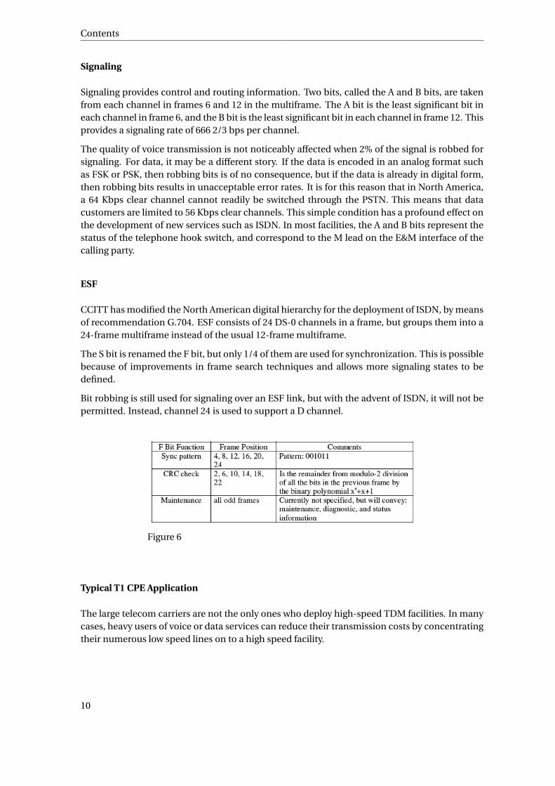
CCITT has modified the North American digital hierarchy for the deployment of ISDN, by meansof recommendation G.704. ESF consists of 24 DS-0 channels in a frame, but groups them into a24-frame multiframe instead of the usual 12-frame multiframe.

The S bit is renamed the F bit, but only 1/4 of them are used for synchronization. This is possiblebecause of improvements in frame search techniques and allows more signaling states to bedefined.

Bit robbing is still used for signaling over an ESF link, but with the advent of ISDN, it will not bepermitted. Instead, channel 24 is used to support a D channel.

Figure 6

Typical T1 CPE Application

The large telecom carriers are not the only ones who deploy high-speed TDM facilities. In manycases, heavy users of voice or data services can reduce their transmission costs by concentratingtheir numerous low speed lines on to a high speed facility.

10

Time Division Multiplexing

There are many types of T1 multiplexers available today. Some are relatively simple devices,while others allow for channel concatenation, thus supporting a wide range of data rates. Theability to support multiple DS-0s allows for easy facilitation of such protocols as the video tele-conferencing standard, Px64.

Figure 7

Multiplexers

Multiplexing units are often designated by the generic term Mab wherea is input DS level and bis the output DS level. Thus, an M13 multiplexer combines 28 DS–1s into a single DS–3 and anM23 multiplexer combines 7 DS–2s into a single DS–3.

11

Contents

Figure 8

ZBTSI

ZBTSI (zero byte time slot interchange) is used on DS–4 links. Four DS-1 frames are loaded intoa register, and renumbered 1–96. If there are any empty slots [all zeros], the first framing bit isinverted and all blank slots are relocated to the front of the frame. Channel 1 is then loaded with a7-bit number corresponding to the original position of the first empty slot. Bit 8 used to indicatewhether the following channel contains user information or another address for an empty slot.

If there is a second vacancy, bit 8 in the previous channel is set, and the empty slot address isplaced in channel 2. This process continues until all empty positions are filled.

The decoding process at the receiver is done in reverse. Borrowing 1 in 4 framing bits for thissystem is not enough to cause loss of synchronization and provides a 64 Kbps clear channel tothe end-user.

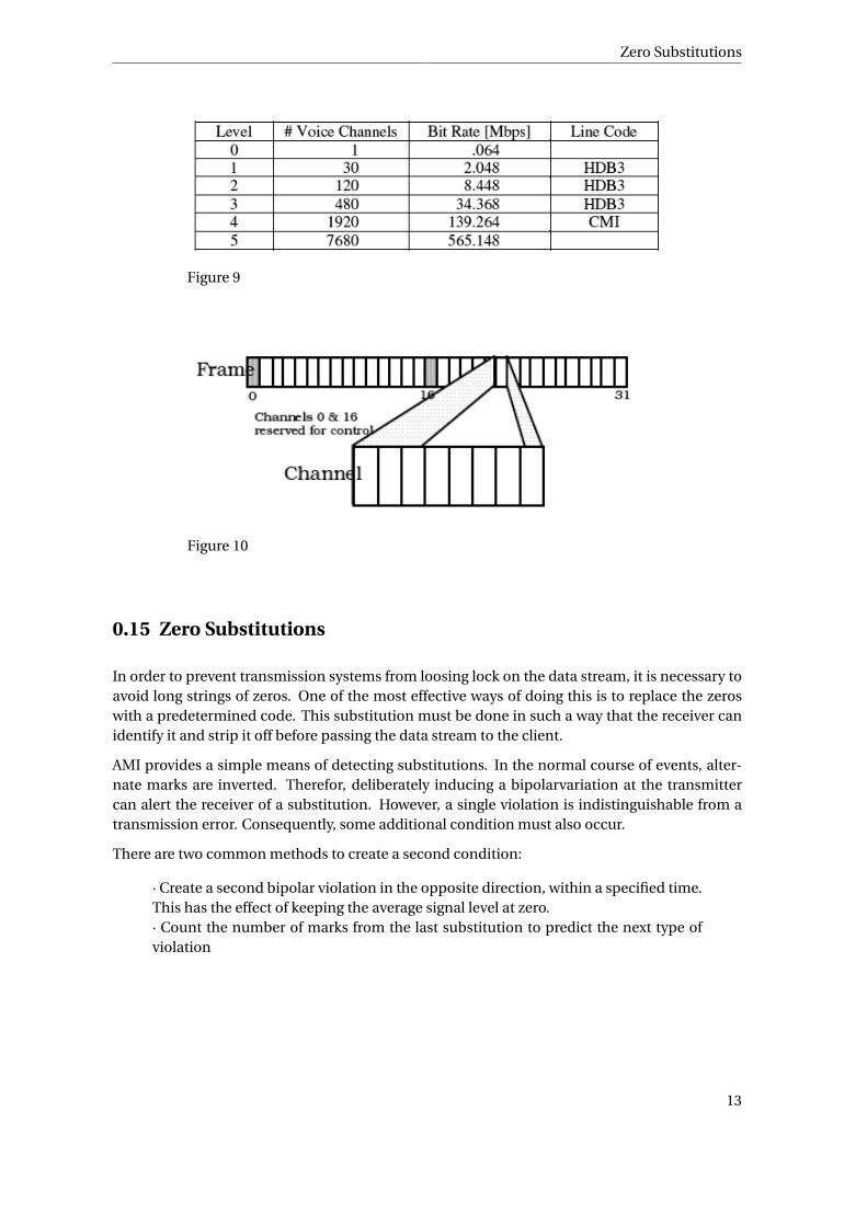
0.14.2 European TDM Carriers

European systems were developed along slightly different principles. The 64 Kbps channel is stillthe basic unit, but signaling is not included in each channel. Instead, common channel signalingis used. In a level 1 carrier, channels 0 and 16 are reserved for signaling and control. This subtledifference means that European systems did not experience the toll fraud and 56 k bottleneckscommon to North American systems, and they experience a much larger penetration of ISDNservices.

12

Zero Substitutions

Figure 9

Figure 10

0.15 Zero Substitutions

In order to prevent transmission systems from loosing lock on the data stream, it is necessary toavoid long strings of zeros. One of the most effective ways of doing this is to replace the zeroswith a predetermined code. This substitution must be done in such a way that the receiver canidentify it and strip it off before passing the data stream to the client.

AMI provides a simple means of detecting substitutions. In the normal course of events, alter-nate marks are inverted. Therefor, deliberately inducing a bipolarvariation at the transmittercan alert the receiver of a substitution. However, a single violation is indistinguishable from atransmission error. Consequently, some additional condition must also occur.

There are two common methods to create a second condition:

· Create a second bipolar violation in the opposite direction, within a specified time.This has the effect of keeping the average signal level at zero.· Count the number of marks from the last substitution to predict the next type ofviolation

13

Contents

0.15.1 B6ZS

B6ZS (binary six zero substitution) is used on T2 AMI transmission links.

Synchronization can be maintained by replacing strings of zeros with bipolar violations. Sincealternate marks have alternate polarity, two consecutive pulses of the same polarity constitute aviolation. Therefor, violations can be substituted for strings of zeros, and the receiver can deter-mine where substitutions were made.

Since the last mark may have been either positive (+) or negative (-), there are two types of sub-stitutions:

Figure 11

These substitutions force two consecutive violations. A single bit error does not create this con-dition.

Figure 12

0.15.2 B8ZS

This scheme uses the same substitution as B6ZS.

Figure 13

14

Zero Substitutions

0.15.3 B3ZS

B3ZS is more involved than B6ZS, and is used on DS–3 carrier systems. The substitution is notonly dependent on the polarity of the last mark, but also on the number of marks since the lastsubstitution.

Figure 14

Figure 15

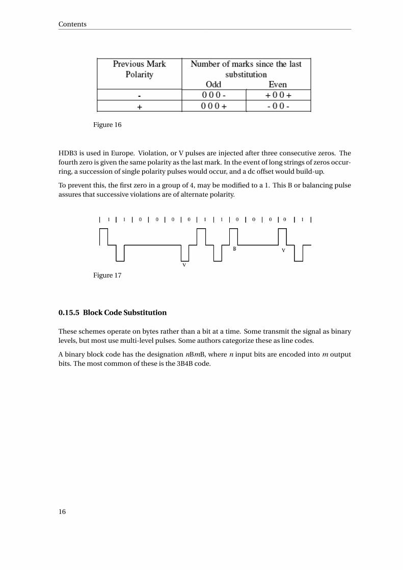
0.15.4 HDB3

HDB3 (high density binary 3) introduces bipolar violations when four consecutive zeros occur. Itcan therefore also be called B4ZS. The second and thirds zeros are left unchanged, but the fourthzero is given the same polarity as the last mark. The first zero may be modified to a one to makesure that successive violations are of alternate polarity.

15

Contents

Figure 16

HDB3 is used in Europe. Violation, or V pulses are injected after three consecutive zeros. Thefourth zero is given the same polarity as the last mark. In the event of long strings of zeros occur-ring, a succession of single polarity pulses would occur, and a dc offset would build-up.

To prevent this, the first zero in a group of 4, may be modified to a 1. This B or balancing pulseassures that successive violations are of alternate polarity.

Figure 17

0.15.5 Block Code Substitution

These schemes operate on bytes rather than a bit at a time. Some transmit the signal as binarylevels, but most use multi-level pulses. Some authors categorize these as line codes.

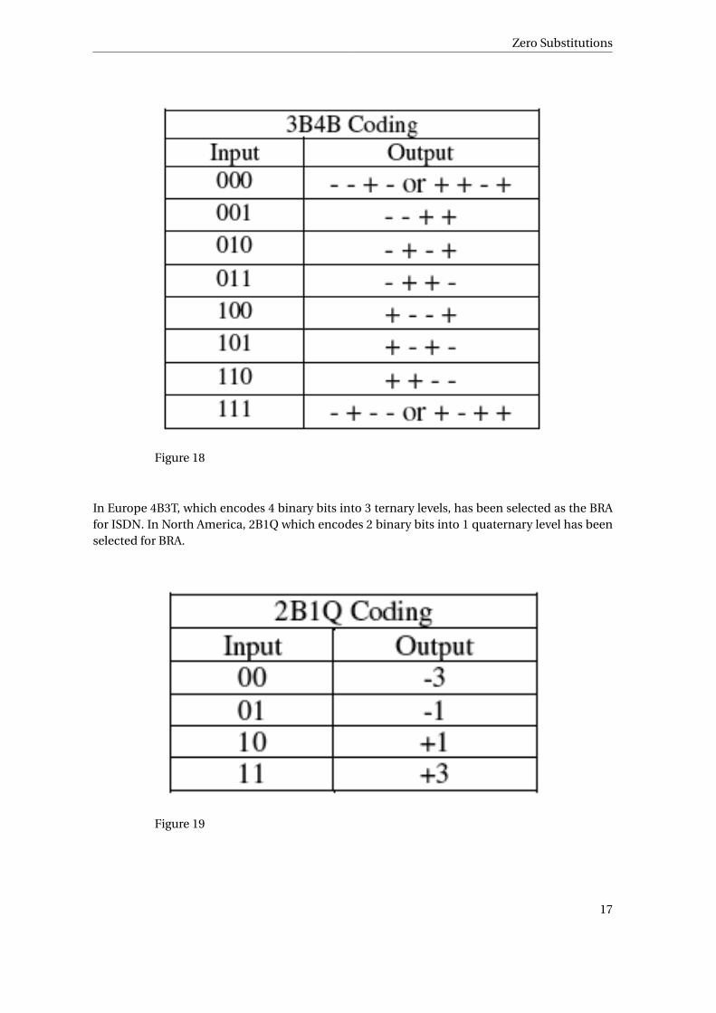
A binary block code has the designation nBmB, where n input bits are encoded into m outputbits. The most common of these is the 3B4B code.

16

Zero Substitutions

Figure 18

In Europe 4B3T, which encodes 4 binary bits into 3 ternary levels, has been selected as the BRAfor ISDN. In North America, 2B1Q which encodes 2 binary bits into 1 quaternary level has beenselected for BRA.

Figure 19

17

Contents

Some block codes do not generate multilevel pulses. For example, 24B1P or 24B25B simply addsa P or parity bit to a 24 bit block.

0.16 Benefits of TDM

TDM is all about cost: fewer wires and simpler receivers are used to transmit data from mul-tiple sources to multiple destinations. TDM also uses less bandwidth than Frequency-DivisionMultiplexing (FDM) signals, unless the bitrate is increased, which will subsequently increase thenecessary bandwidth of the transmission.

0.17 Synchronous TDM

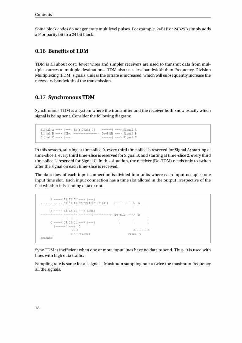
Synchronous TDM is a system where the transmitter and the receiver both know exactly whichsignal is being sent. Consider the following diagram:

Signal A ---> |---| |A|B|C|A|B|C| |------| ---> Signal ASignal B ---> |TDM| --------------> |De-TDM| ---> Signal BSignal C ---> |---| |------| ---> Signal C

In this system, starting at time-slice 0, every third time-slice is reserved for Signal A; starting attime-slice 1, every third time-slice is reserved for Signal B; and starting at time-slice 2, every thirdtime-slice is reserved for Signal C. In this situation, the receiver (De-TDM) needs only to switchafter the signal on each time-slice is received.

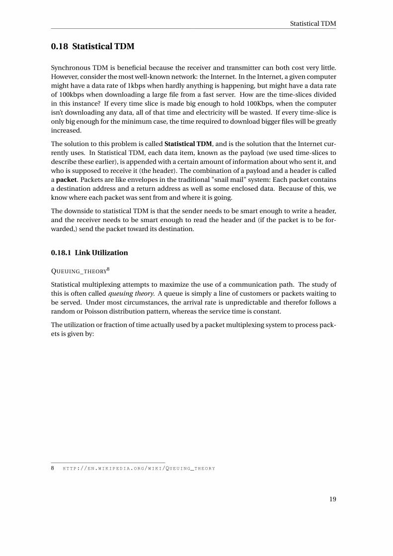
The data flow of each input connection is divided into units where each input occupies oneinput time slot. Each input connection has a time slot alloted in the output irrespective of thefact whether it is sending data or not.

A -----|A3|A2|A1|---> |---|.............|C3|B3|A3|C2|B2|A2|C1|B1|A1| |------| ---> A

| | | | | | |B -----|B3|B2|B1|---> |MUX|

-------------|--------|--------|----------> |De-MUX| ---> B| | | | | | |

C -----|C3|C2|C1|---> |---| | | ||------| ---> C

<--> <-------->Bit Interval Frame (x

seconds)

Sync TDM is inefficient when one or more input lines have no data to send. Thus, it is used withlines with high data traffic.

Sampling rate is same for all signals. Maximum sampling rate = twice the maximum frequencyall the signals.

18

Statistical TDM

0.18 Statistical TDM

Synchronous TDM is beneficial because the receiver and transmitter can both cost very little.However, consider the most well-known network: the Internet. In the Internet, a given computermight have a data rate of 1kbps when hardly anything is happening, but might have a data rateof 100kbps when downloading a large file from a fast server. How are the time-slices dividedin this instance? If every time slice is made big enough to hold 100Kbps, when the computerisn’t downloading any data, all of that time and electricity will be wasted. If every time-slice isonly big enough for the minimum case, the time required to download bigger files will be greatlyincreased.

The solution to this problem is called Statistical TDM, and is the solution that the Internet cur-rently uses. In Statistical TDM, each data item, known as the payload (we used time-slices todescribe these earlier), is appended with a certain amount of information about who sent it, andwho is supposed to receive it (the header). The combination of a payload and a header is calleda packet. Packets are like envelopes in the traditional "snail mail" system: Each packet containsa destination address and a return address as well as some enclosed data. Because of this, weknow where each packet was sent from and where it is going.

The downside to statistical TDM is that the sender needs to be smart enough to write a header,and the receiver needs to be smart enough to read the header and (if the packet is to be for-warded,) send the packet toward its destination.

0.18.1 Link Utilization

QUEUING_THEORY8

Statistical multiplexing attempts to maximize the use of a communication path. The study ofthis is often called queuing theory. A queue is simply a line of customers or packets waiting tobe served. Under most circumstances, the arrival rate is unpredictable and therefor follows arandom or Poisson distribution pattern, whereas the service time is constant.

The utilization or fraction of time actually used by a packet multiplexing system to process pack-ets is given by:

8 HTTP://EN.WIKIPEDIA.ORG/WIKI/QUEUING_THEORY

19

Contents

Figure 20

The queue length or average number of items waiting to be served is given by:

q = ρ2

2(1−ρ) +ρ

20

Statistical TDM

Figure 21

Example

A T1 link has been divided into a number of 9.6 Kbps channels and has acombined user data rate of 1.152 Mbps. Access to this channel is offeredto 100 customers, each requiring 9.6 Kbps data 20% of the time. If the userarrival time is strictly random find the T1 link utilization.

Solution

The utilization or fraction of time used by the system to process packetsis given by:

ρ = αN R

M= 0.2×100×9.6×103

1.152×106 = 0.167

A 24 channel system dedicated to DATA, can place five 9.6 Kbps customersin each of 23 channels, for a total of 115 customers. In the above statisticallink, 100 customers created an average utilization of 0.167 and were easilyfitted, with room to spare if they transmit on the average 20% of the time.If however, the customer usage were not randomly distributed, then theabove analysis would have to be modified.

21

Contents

This example shows the potential for statistical multiplexing. If channels were assigned on a de-mand basis (only when the customer had something to send), a single T1 may be able to supporthundreds of low volume users.

A utilization above 0.8 is undesirable in a statistical system, since the slightest variation in cus-tomer requests for service would lead to buffer overflow. Service providers carefully monitordelay and utilization and assign customers to maximize utilization and minimize cost.

0.19 Packets

Packets will be discussed in greater detail once we start talking about digital networks (specifi-cally the Internet). Packet headers not only contain address information, but may also include anumber of different fields that will display information about the packet. Many headers containerror-checking information (checksum, Cyclic Redundancy Check) that enables the receiver tocheck if the packet has had any errors due to interference, such as electrical noise.

0.20 Duty Cycles

Duty cycle is defined as " the time that is effectively used to send or receive the data, expressed asa percentage of total period of time." The more the duty cycle , the more effective transmissionor reception.

We can define the pulse width, τ, as being the time that a bit occupies from within its total allotedbit-time Tb. If we have a duty cycle of D, we can define the pulse width as:

τ= DTb

Where:

0 < τ≤ Tb

The pulse width is equal to the bit time if we are using a 100% duty cycle.

0.21 Introduction

It turns out that many wires have a much higher bandwidth than is needed for the signals thatthey are currently carrying. Analog Telephone transmissions, for instance, require only 3 000Hz of bandwidth to transmit human voice signals. Over short distances, however, twisted-pairtelephone wire has an available bandwidth of nearly 100 000 Hz!

There are several terrestrial radio based communications systems deployed today. They include:

• Cellular radio• Mobile radio

22

Introduction

• Digital microwave radio

Mobile radio service was first introduced in the St. Louis in 1946. This system was essentiallya radio dispatching system with an operator who was able to patch the caller to the PSTN viaa switchboard. Later, an improved mobile telephone system, IMTS, allowed customers to dialtheir own calls without the need for an operator. This in turn developed into the cellular radionetworks we see today.

The long haul PSTNs and packet data networks use a wide variety of transmission media includ-ing

• Terrestrial microwave• Satellite microwave• Fiber optics• Coaxial cable

In this section, we will be concerned with terrestrial microwave systems. Originally, microwavelinks used FDM exclusively as the access technique, but recent developments are changing ana-log systems to digital where TDM is more appropriate.

0.21.1 Fixed Access Assignment

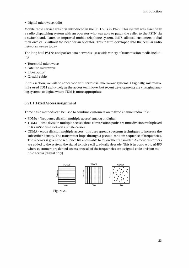
Three basic methods can be used to combine customers on to fixed channel radio links:

• FDMA - (frequency division multiple access) analog or digital• TDMA - (time division multiple access) three conversation paths are time division multiplexed

in 6.7 mSec time slots on a single carrier.• CDMA - (code division multiple access) this uses spread spectrum techniques to increase the

subscriber density. The transmitter hops through a pseudo-random sequence of frequencies.The receiver is given the sequence list and is able to follow the transmitter. As more customersare added to the system, the signal to noise will gradually degrade. This is in contrast to AMPSwhere customers are denied access once all of the frequencies are assigned code division mul-tiple access [digital only]

Figure 22

23

Contents

0.22 What is FDM?

FREQUENCY-DIVISION_MULTIPLEXING9

Frequency Division Multiplexing (FDM) allows engineers to utilize the extra space in each wireto carry more than one signal. By frequency-shifting some signals by a certain amount, engineerscan shift the spectrum of that signal up into the unused band on that wire. In this way, multi-ple signals can be carried on the same wire, without having to divy up time-slices as in Time-Division Multiplexing schemes.In analog transmission, signals are commonly multiplexed usingfrequency-division multiplexing (FDM), in which the carrier bandwidth is divided into subchan-nels of different frequency widths, each carrying a signal at the same time in parallel

i Information

Broadcast radio and television channels are separated in the frequency spectrum usingFDM. Each individual channel occupies a finite frequency range, typically some multipleof a given base frequency.

Traditional terrestrial microwave and satellite links employ FDM. Although FDM in telecommu-nications is being reduced, several systems will continue to use this technique, namely: broad-cast & cable TV, and commercial & cellular radio.

0.22.1 Analog Carrier Systems

The standard telephony voice band [300 – 3400 Hz] is heterodyned and stacked on high fre-quency carriers by single sideband amplitude modulation. This is the most bandwidth efficientscheme possible.

Figure 23

The analog voice channels are pre-grouped into threes and heterodyned on carriers at 12, 16, and20 kHz. The resulting upper sidebands of four such pregroups are then heterodyned on carriersat 84, 96, 108, and 120 kHz to form a 12-channel group.

Since the lower sideband is selected in the second mixing stage, the channel sequence is reversedand a frequency inversion occurs within each channel.

9 HTTP://EN.WIKIPEDIA.ORG/WIKI/%20FREQUENCY-DIVISION_MULTIPLEXING

24

What is FDM?

Figure 24

This process can continue until the available bandwidth on the coaxial cable or microwave linkis exhausted.

Figure 25

In the North American system, there are:

• 12 channels per group• 5 groups per supergroup• 10 super groups per mastergroup• 6 master groups per jumbogroup

In the European CCITT system, there are:

• 12 channels per group• 5 groups per supergroup• 5 super groups per mastergroup• 3 master groups per supermastergroup

There are other FDM schemes including:

• L600 - 600 voice channels 60–2788 kHz• U600 - 600 voice channels 564–3084 kHz• L3 - 1860 voice channels 312–8284 kHz, comprised of 3 mastergroups and a supergroup• L4 - 3600 voice channels, comprised of six U600s

25

Contents

0.23 Benefits of FDM

FDM allows engineers to transmit multiple data streams simultaneously over the same chan-nel, at the expense of bandwidth. To that extent, FDM provides a trade-off: faster data for lessbandwidth. Also, to demultiplex an FDM signal requires a series of bandpass filters to isolateeach individual signal. Bandpass filters are relatively complicated and expensive, therefore thereceivers in an FDM system are generally expensive.

0.24 Examples of FDM

As an example of an FDM system, Commercial broadcast radio (AM and FM radio) simultane-ously transmits multiple signals or "stations" over the airwaves. These stations each get theirown frequency band to use, and a radio can be tuned to receive each different station. Anothergood example is cable television, which simultaneously transmits every channel, and the TV"tunes in" to which channel it wants to watch.

0.25 Orthogonal FDM

ORTHOGONAL_FREQUENCY-DIVISION_MULTIPLEXING10

Orthogonal Frequency Division Multiplexing (OFDM) is a more modern variant of FDM that usesorthogonal sub-carriers to transmit data that does not overlap in the frequency spectrum and isable to be separated out using frequency methods. OFDM has a similar data rate to traditionalFDM systems, but has a higher resilience to disruptive channel conditions such as noise andchannel fading.

0.26 Voltage Controlled Oscillators (VCO)

VOLTAGE-CONTROLLED_OSCILLATOR11

A voltage-controlled oscillator (VCO) is a device that outputs a sinusoid of a frequency that is afunction of the input voltage. VCOs are not time-invariant, linear components. A complete studyof how a VCO works will probably have to be relegated to a book on electromagnetic phenomena.This page will, however, attempt to answer some of the basic questions about VCOs.

A basic VCO has input/output characteristics as such:

v(t) ----|VCO|----> sin(a[f + v(t)]t + O)

VCOs are often implemented using a special type of diode called a "Varactor". Varactors, whenreverse-biased, produce a small amount of capacitance that varies with the input voltage.

10 HTTP://EN.WIKIPEDIA.ORG/WIKI/ORTHOGONAL_FREQUENCY-DIVISION_MULTIPLEXING11 HTTP://EN.WIKIPEDIA.ORG/WIKI/VOLTAGE-CONTROLLED_OSCILLATOR

26

Phase-Locked Loops

0.27 Phase-Locked Loops

PHASE-LOCKED_LOOP12

If you are talking on your cellphone, and you are walking (or driving), the phase angle of yoursignal is going to change, as a function of your motion, at the receiver. This is a fact of nature,and is unavoidable. The solution to this then, is to create a device which can "find" a signal of aparticular frequency, negate any phase changes in the signal, and output the clean wave, phase-change free. This device is called a Phase-Locked Loop (PLL), and can be implemented using aVCO.

0.28 Purpose of VCO and PLL

VCO and PLL circuits are highly useful in modulating and demodulating systems. We will discussthe specifics of how VCO and PLL circuits are used in this manner in future chapters.

0.29 Varactors

As a matter of purely professional interest, we will discuss varactors here.

0.30 Further reading

• CLOCK AND DATA RECOVERY13 has detailed information about designing and analyzing PLLs.(VCO)

0.31 What is an Envelope Filter?

If anybody has some images that they can upload, it would be much better then these ASCII artthings.

The envelope detector is a simple analog circuit that can be used to find the peaks in a quickly-changing waveform. Envelope detectors are used in a variety of devices, specifically becausepassing a sinusoid through an envelope detector will suppress the sinusoid.

12 HTTP://EN.WIKIPEDIA.ORG/WIKI/PHASE-LOCKED_LOOP13 HTTP://EN.WIKIBOOKS.ORG/WIKI/CLOCK%20AND%20DATA%20RECOVERY

27

Contents

0.32 Circuit Diagram

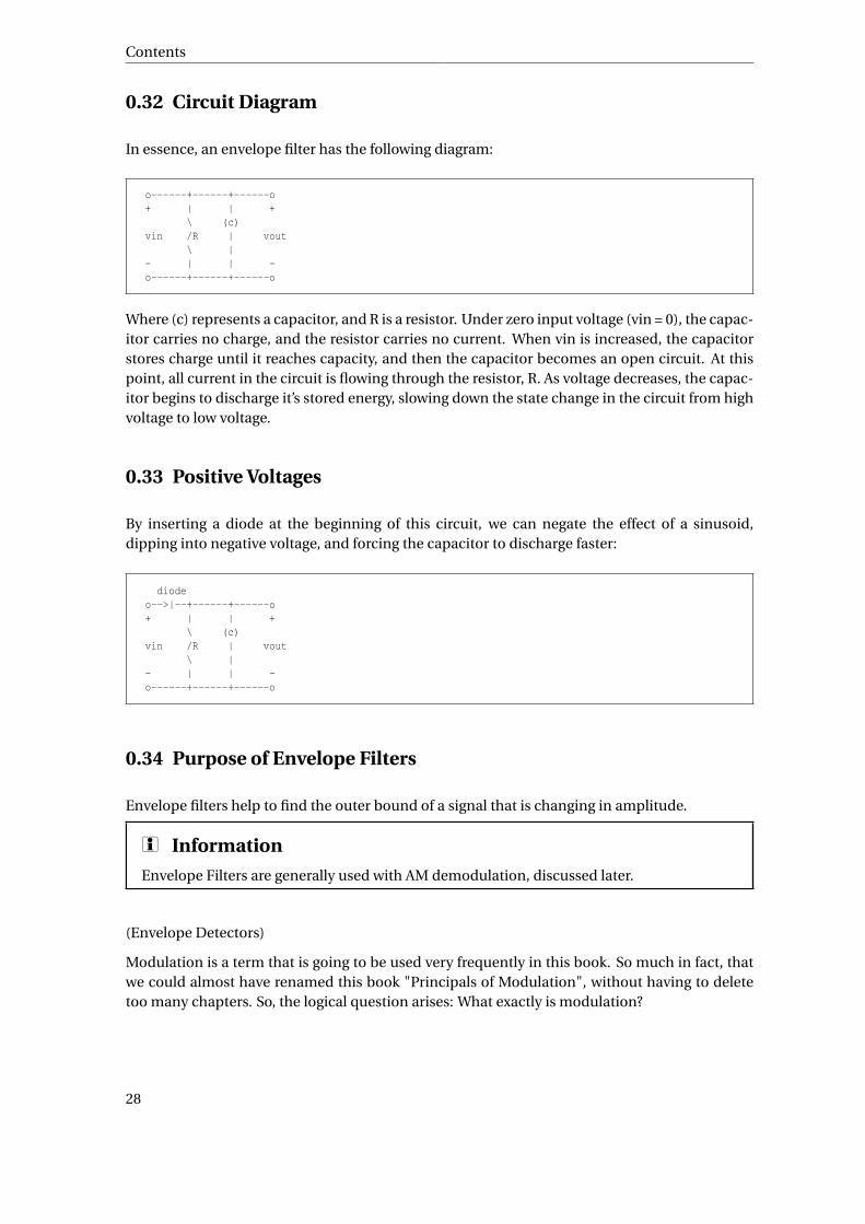
In essence, an envelope filter has the following diagram:

o------+------+------o+ | | +

\ (c)vin /R | vout

\ |- | | -o------+------+------o

Where (c) represents a capacitor, and R is a resistor. Under zero input voltage (vin = 0), the capac-itor carries no charge, and the resistor carries no current. When vin is increased, the capacitorstores charge until it reaches capacity, and then the capacitor becomes an open circuit. At thispoint, all current in the circuit is flowing through the resistor, R. As voltage decreases, the capac-itor begins to discharge it’s stored energy, slowing down the state change in the circuit from highvoltage to low voltage.

0.33 Positive Voltages

By inserting a diode at the beginning of this circuit, we can negate the effect of a sinusoid,dipping into negative voltage, and forcing the capacitor to discharge faster:

diodeo-->|--+------+------o+ | | +

\ (c)vin /R | vout

\ |- | | -o------+------+------o

0.34 Purpose of Envelope Filters

Envelope filters help to find the outer bound of a signal that is changing in amplitude.

i Information

Envelope Filters are generally used with AM demodulation, discussed later.

(Envelope Detectors)

Modulation is a term that is going to be used very frequently in this book. So much in fact, thatwe could almost have renamed this book "Principals of Modulation", without having to deletetoo many chapters. So, the logical question arises: What exactly is modulation?

28

Definition

0.35 Definition

Modulation is a process of mixing a signal with a sinusoid to produce a new signal. This new sig-nal, conceivably, will have certain benefits of an un-modulated signal, especially during trans-mission. If we look at a general function for a sinusoid:

f (t ) = A sin(ωt +φ)

we can see that this sinusoid has 3 parameters that can be altered, to affect the shape of thegraph. The first term, A, is called the magnitude, or amplitude of the sinusoid. The next term, ωis known as the frequency, and the last term, φ is known as the phase angle. All 3 parameters canbe altered to transmit data.

The sinusoidal signal that is used in the modulation is known as the carrier signal, or simply "thecarrier". The signal that is used in modulating the carrier signal(or sinusoidal signal) is knownas the "data signal" or the "message signal". It is important to notice that a simple sinusoidalcarrier contains no information of its own.

In other words we can say that modulation is used because the some data signals are not alwayssuitable for direct transmission, but the modulated signal may be more suitable.

0.36 Types of Modulation

There are 3 basic types of modulation: Amplitude modulation, Frequency modulation, andPhase modulation.

amplitude modulation

a type of modulation where the amplitude of the carrier signal is modulated(changed) in proportion to the message signal while the frequency and phase arekept constant.

frequency modulation

a type of modulation where the frequency of the carrier signal is modulated(changed) in proportion to the message signal while the amplitude and phase arekept constant.

phase modulation

a type of modulation where the phase of the carrier signal is modulated (changed) inproportion to the message signal while the amplitude and frequency are kept con-stant.

29

Contents

0.37 Why Use Modulation?

Clearly the concept of modulation can be a little tricky, especially for the people who don’t liketrigonometry. Why then do we bother to use modulation at all? To answer this question, let’sconsider a channel that essentially acts like a bandpass filter: The lowest frequency componentsand the highest frequency components are attenuated or unusable, in some way. If we can’t sendlow-frequency signals, then we need to shift our signal up the frequency ladder. Modulation al-lows us to send a signal over a bandpass frequency range. If every signal gets its own frequencyrange, then we can transmit multiple signals simultaneously over a single channel, all using dif-ferent frequency ranges.

Another reason to modulate a signal is to allow the use of a smaller antenna. A baseband (lowfrequency) signal would need a huge antenna because in order to be efficient, the antenna needsto be about 1/10th the length of the wavelength. Modulation shifts the baseband signal up toa much higher frequency, which has much smaller wavelengths and allows the use of a muchsmaller antenna.

0.38 Examples

Think about your car radio. There are more than a dozen (or so) channels on the radio at anytime, each with a given frequency: 100.1MHz, 102.5MHz etc... Each channel gets a certain range(usually about 0.2MHz), and the entire station gets transmitted over that range. Modulationmakes it all possible, because it allows us to send voice and music (which are essentiall basebandsignals) over a bandpass (or "Broadband") channel.

0.39 non-sinusoidal modulation

A sine wave at one frequency can be separated from a sine wave at another frequency (or a cosinewave at the same frequency) because the two signals are "orthogonal".

There are other sets of signals, such that every signal in the set is orthogonal to every other signalin the set.

A simple orthogonal set is time multiplexed division (TDM) -- only one transmitter is active atany one time.

Other more complicated sets of orthogonal waveforms -- Walsh codes and various pseudonoisecodes such as Gold codes and maximum length sequences -- are also used in some communica-tion systems.

The process of combining these waveforms with data signals is sometimes called "modulation",because it is so very similar to the way modulation combines sine waves are with data signals.

30

further reading

0.40 further reading

• DATA CODING THEORY/SPECTRUM SPREADING14

• WIKIPEDIA:WALSH CODE15

• WIKIPEDIA:GOLD CODE16

• WIKIPEDIA:PSEUDONOISE CODE17

• WIKIPDIA:MAXIMUM LENGTH SEQUENCE18

There is lots of talk nowadays about buzzwords such as "Analog" and "Digital". Certainly, engi-neers who are interested in creating a new communication system should understand the dif-ference. Which is better, analog or digital? What is the difference? What are the pros and cons ofeach? This chapter will look at the answers to some of these questions.

0.41 What are They?

What exactly is an analog signal, and what is a digital signal?

Analog : Analog signals are signals with continuous values. Analog signals are used in manysystems, although the use of analog signals has declined with the advent of cheap digitalsignals.

Digital : Digital signals are signals that are represented by binary numbers, "1" or "0". The 1and 0 values can correspond to different discrete voltage values, and any signal that doesntquite fit into the scheme just gets rounded off.

0.42 What are the Pros and Cons?

Each paradigm has its own benefits and problems.

Analog : Analog systems are less tolerant to noise, make good use of bandwidth, and are easyto manipulate mathematically. However, analog signals require hardware receivers andtransmitters that are designed to perfectly fit the particular transmission. If you are work-ing on a new system, and you decide to change your analog signal, you need to completelychange your transmitters and receivers.

Digital : Digital signals are more tolerant to noise, but digital signals can be completely cor-rupted in the presence of excess noise. In digital signals, noise could cause a 1 to be inter-preted as a 0 and vice versa, which makes the received data different than the original data.Imagine if the army transmitted a position coordinate to a missile digitally, and a single bitwas received in error? This single bit error could cause a missile to miss its target by miles.Luckily, there are systems in place to prevent this sort of scenario, such as checksums and

14 HTTP://EN.WIKIBOOKS.ORG/WIKI/DATA%20CODING%20THEORY%2FSPECTRUM%20SPREADING15 HTTP://EN.WIKIPEDIA.ORG/WIKI/WALSH%20CODE16 HTTP://EN.WIKIPEDIA.ORG/WIKI/GOLD%20CODE17 HTTP://EN.WIKIPEDIA.ORG/WIKI/PSEUDONOISE%20CODE18 HTTP://EN.WIKIBOOKS.ORG/WIKI/WIKIPDIA%3AMAXIMUM%20LENGTH%20SEQUENCE

31

Contents

CRCs, which tell the receiver when a bit has been corrupted and ask the transmitter to re-send the data. The primary benefit of digital signals is that they can be handled by simple,standardized receivers and transmitters, and the signal can be then dealt with in software(which is comparatively cheap to change).

The Difference between Digital and Discrete:

Digital quantity may be either 0 or 1, but discrete may be any numerical value i.e. 0,1....9.

0.43 Sampling and Reconstruction

The process of converting from analog data to digital data is called "sampling". The process ofrecreating an analog signal from a digital one is called "reconstruction". This book will not talkabout either of these subjects in much depth beyond this, although other books on the topic ofEE might, such as A-LEVEL PHYSICS (ADVANCING PHYSICS)/DIGITISATION19.

0.44 further reading

• ELECTRONICS/DIGITAL TO ANALOG & ANALOG TO DIGITAL CONVERTERS20

Signals need a channel to follow, so that they can move from place to place. These Communi-cation Mediums, or "channels" are things like wires and antennae that transmit the signal fromone location to another. Some of the most common channels are listed below:

0.45 Twisted Pair Wire

TWISTED PAIR21 Twisted Pair is a transmission medium that uses two conductors that are twistedtogether to form a pair. The concept for the twist of the conductors is to prevent interference.Ideally, each conductor of the pair basically receives the same amount of interference, positiveand negative, effectively cancelling the effect of the interference. Typically, most inside cablinghas four pairs with each pair having a different twist rate. The different twist rates help to furtherreduce the chance of crosstalk by making the pairs appear electrically different in reference toeach other. If the pairs all had the same twist rate, they would be electrically identical in referenceto each other causing crosstalk, which is also referred to as capacitive coupling. Twisted pair wireis commonly used in telephone and data cables with variations of categories and twist rates.

SHIELDED TWISTED PAIR22 Other variants of Twisted Pair are the Shielded Twisted Pair cables.The shielded types operate very similar to the non-shielded variety, except that Shielded TwistedPair also has a layer of metal foil or mesh shielding around all the pairs or each individual pair to

19 HTTP://EN.WIKIBOOKS.ORG/WIKI/A-LEVEL%20PHYSICS%20%28ADVANCING%20PHYSICS%29%2FDIGITISATION

20 HTTP://EN.WIKIBOOKS.ORG/WIKI/ELECTRONICS%2FDIGITAL%20TO%20ANALOG%20%26%20ANALOG%20TO%20DIGITAL%20CONVERTERS

21 HTTP://EN.WIKIPEDIA.ORG/WIKI/TWISTED%20PAIR22 HTTP://EN.WIKIPEDIA.ORG/WIKI/SHIELDED%20TWISTED%20PAIR

32

Coaxial Cable

further shield the pairs from electromagnetic interference. Shielded twisted pair is typically de-ployed in situations where the cabling is subjected to higher than normal levels of interference.

0.46 Coaxial Cable

COAXIAL CABLE23 Another common type of wire is Coaxial Cable. Coaxial cable (or simply,"coax") is a type of cable with a single data line, surrounded by various layers of padding andshielding. The most common coax cable, common television cable, has a layer of wire mesh sur-rounding the padded core, that absorbs a large amount of EM interference, and helps to ensurea relatively clean signal is transmitted and received. Coax cable has a much higher bandwidththan a twisted pair, but coax is also significantly more expensive than an equal length of twistedpair wire. Coax cable frequently has an available bandwidth in excess of hundreds of megahertz(in comparison with the hundreds of kilohertz available on twisted pair wires).

Originally, Coax cable was used as the backbone of the telephone network because a single coax-ial cable could hold hundreds of simultaneous phone calls by a method known as "FrequencyDivision Multiplexing" (discussed in a later chapter). Recently however, Fiber Optic cables havereplaced Coaxial Cable as the backbone of the telephone network because Fiber Optic channelscan hold many more simultaneous phone conversations (thousands at a time), and are less sus-ceptible to interference, crosstalk, and noise then Coaxial Cable.

0.47 Fiber Optics

GLASS FIBERS24 Fiber Optic cables are thin strands of glass that carry pulses of light (frequentlyinfrared light) across long distances. Fiber Optic channels are usually immune to common RFinterference, and can transmit incredibly high amounts of data very quickly. There are 2 generaltypes of fiber optic cable: single frequency cable, and multi-frequency cable. single frequencycable carries only a single frequency of laser light, and because of this there is no self-interferenceon the line. Single-frequency fiber optic cables can attain incredible bandwidths of many giga-hertz. Multi-Frequency fiber optics cables allow a Frequency-Division Multiplexed series of sig-nals to each inhabit a given frequency range. However, interference between the different signalscan decrease the range over which reliable data can be transmitted.

0.48 Wireless Transmission

In wireless transmission systems, signals are propagated as Electro-Magnetic waves throughfree space. Wireless signals are transmitted by a transmitter, and received by a receiver. Wirelesssystems are inexpensive because no wires need to be installed to transmit the signal, but wire-less transmissions are susceptible not only to EM interference, but also to physical interference.

23 HTTP://EN.WIKIPEDIA.ORG/WIKI/COAXIAL%20CABLE24 HTTP://EN.WIKIPEDIA.ORG/WIKI/GLASS%20FIBERS

33

Contents

A large building in a city, for instance can interfere with cell-phone reception, and a large moun-tain could block AM radio transmissions. Also, WiFi internet users may have noticed that theirwireless internet signals don’t travel through walls very well.

There are 2 types of antennas that are used in wireless communications, isotropic, and direc-tional.

0.48.1 Isotropic

People should be familiar with isotropic antennas because they are everywhere: in your car, onyour radio, etc... Isotropic antennas are omni-directional in the sense that they transmit dataout equally (or nearly equally) in all directions. These antennas are excellent for systems (suchas FM radio transmission) that need to transmit data to multiple receivers in multiple directions.Also, Isotropic antennas are good for systems in which the direction of the receiver, relative tothe transmitter is not known (such as cellular phone systems).

0.48.2 Directional

Directional antennas focus their transmission power in a single narrow direction range. Someexamples of directional antennas are satellite dishes, and wave-guides. The downfall of the di-rectional antennas is that they need to be pointed directly at the receiver all the time to maintaintransmission power. This is useful when the receiver and the transmitter are not moving (suchas in communicating with a geo-synchronous satellite).

0.49 Receiver Design

It turns out that if we know what kind of signal to expect, we can better receive those signals. Thisshould be intuitive, because it is hard to find something if we don’t know what precisely we arelooking for. How is a receiver supposed to know what is data and what is noise, if it doesnt knowwhat data looks like?

Coherent transmissions are transmissions where the receiver knows what type of data is beingsent. Coherency implies a strict timing mechanism, because even a data signal may look likenoise if you look at the wrong part of it. In contrast, noncoherent receivers don’t know exactlywhat they are looking for, and therefore noncoherent communication systems need to be farmore complex (both in terms of hardware and mathematical models) to operate properly.

This section will talk about coherent receivers, first discussing the "Simple Receiver" case, andthen going into theory about what the optimal case is. Once we know mathematically what anoptimal receiver should be, we then discuss two actual implementations of the optimal receiver.

It should be noted that the remainder of this book will discuss optimal receivers. After all, whywould a communication’s engineer use anything that is less than the best?

34

The Simple Receiver

0.50 The Simple Receiver

A simple receiver is just that: simple. A general simple receiver will consist of a low-pass filter(to remove excess high-frequency noise), and then a sampler, that will select values at certainpoints in the wave, and interpolate those values to form a smooth output curve. In place ofa sampler (for purely analog systems), a general envelope filter can also be used, especially inAM systems. In other systems, different tricks can be used to demodulate an input signal, andacquire the data. However simple receivers, while cheap, are not the best choice for a receiver.Occcasionally they are employed because of their price, but where performance is an issue, abetter alternative receiver should be used.

0.51 The Optimal Receiver

Mathematically, Engineers were able to predict the structure of the optimal receiver. Read thatsentence again: Engineers are able to design, analyze, and build the best possible receiver, forany given signal. This is an important development for several reasons. First, it means that nomore research should go into finding a better receiver. The best receiver has already been found,after all. Second, it means any communications system will not be hampered (much) by thereceiver.

0.51.1 Derivation

here we will attempt to show how the coherent receiver is derived.

0.51.2 Matched Receiver

The matched receiver is the logical conclusion of the optimal receiver calculation. The matchedreceiver convolutes the signal with itself, and then tests the output. Here is a diagram:

s(t)----->(Convolve with r(t))----->

This looks simple enough, except that convolution modules are often expensive. An alternativeto this approach is to use a correlation receiver.

0.51.3 Correlation Receiver

The correlation receiver is similar to the matched receiver, instead with a simple switch: Themultiplication happens first, and the integration happens second.

Here is a general diagram:

35

Contents

r(t)|v

s(t) ----->(X)----->(Integrator)--->

In a digital system, the integrator would then be followed by a threshold detector, while in ananalog receiver, it might be followed by another detector, like an envelope detector.

0.52 Conclusion

To do the best job of receiving a signal, we need to know the form of the signal that we are send-ing. This should seem obvious, we can’t design a receiver until after we’ve decided how the signalwill be sent. This method poses some problems however, in that the receiver must be able to lineup the received signal with the given reference signal to work the magic: If the received signaland the reference signal are out of sync with each other, either as a function of an error in phaseor an error in frequency, then the optimal receiver will not work.

0.53 further reading

DEMODULATION25

0.53.1 Section 2: Analog Modulation

0.54 Analog Modulation Overview

Let’s take a look at a generalized sinewave:

x (t ) = A sin(ωt +θ)

It consists of three components namely; amplitude, frequency and phase. Each of which can bedecomposed to provide finer detail:

x(t ) = As(t )sin(2π[ fc +k fm(t )]t +αφ(t ))

0.55 Types of Analog Modulation

We can see 3 parameters that can be changed in this sine wave to send information:

25 HTTP://EN.WIKIPEDIA.ORG/WIKI/DEMODULATION

36

The Breakdown

• As(t ). This term is called the "Amplitude", and changing it is called "Amplitude Modulation"(AM)

• k fm(t ) This term is called the "Frequency Shift", and changing it is called "Frequency Modu-lation"

• αφ(t ). this term is called the "Phase angle", and changing it is called "Phase Modulation".• The terms frequency and phase modulation are often combined into a more general group

called "Angle Modulation".

0.56 The Breakdown

Each term consists of a coefficient (called a "scaling factor"), and a function of time that corre-sponds to the information that we want to send. The scaling factor out front, A, is also used asthe transmission power coefficient. When a radio station wants their signal to be stronger (re-gardless of whether it is AM, FM, or PM), they "crank-up" the power of A, and send more powerout onto the airwaves.

0.57 How we Will Cover the Material

We are going to go into separate chapters for each different type of modulation. This book willattempt to discuss some of the mathematical models and techniques used with different mod-ulation techniques. It will also discuss some practical information about how to construct atransmitter/receiver, and how to use each modulation technique effectively.

Amplitude modulation is one of the earliest radio modulation techniques. The receivers usedto listed to AM-DSB-C are perhaps the simplest receivers of any radio modulation technique;which may be why that version of amplitude modulation is still widely used today. By the end ofthis module, you will know the most popular versions of amplitude modulation, some popularAM modulation circuits, and some popular AM demodulation circuits.

0.58 Amplitude Modulation

AMPLITUDE_MODULATION26

Amplitude modulation (AM) occurs when the amplitude of a carrier wave is modulated, to cor-respond to a source signal. In AM, we have an equation that looks like this:

Fsi g nal (t ) = A(t )sin(ωt )

We can also see that the phase of this wave is irrelevant, and does not change (so we don’t eveninclude it in the equation).

26 HTTP://EN.WIKIPEDIA.ORG/WIKI/AMPLITUDE_MODULATION

37

Contents

i Information

AM Radio uses AM modulation

AM Double-Sideband (AM-DSB for short) can be broken into two different, distinct types: Car-rier, and Suppressed Carrier varieties (AM-DSB-C and AM-DSB-SC, for short, respectively). Thispage will talk about both varieties, and will discuss the similarities and differences of each.

Figure 26

0.58.1 Characteristics

Modulation Index

Amplitude modulation requires a high frequency constant carrier and a low frequency modula-tion signal.

A sine wave carrier is of the form

ec = Ec sin(ωc t )

A sine wave modulation signal is of the form

em = Em sin(ωm t )

Notice that the amplitude of the high frequency carrier takes on the shape of the lower frequencymodulation signal, forming what is called a modulation envelope.

38

Amplitude Modulation

Figure 27

The modulation index is defined as the ratio of the modulation signal amplitude to the carrieramplitude.

mam = Em

Ec

where0 ≤ mam ≤ 1

The overall signal can be described by:

eam = (Ec +Em sin(ωm t ))sin(ωc t )

More commonly, the carrier amplitude is normalized to one and the am equation is written as:

eam = (1+mam sin(ωm t ))sin(ωc t )

In most literature this expression is simply written as:

e = (1+m sinωm t )sinωc t

If the modulation index is zero (mam = 0

) the signal is simply a constant amplitude carrier.

If the modulation index is 1 (mam = 1

), the resultant waveform has maximum or 100% amplitude modulation.

39

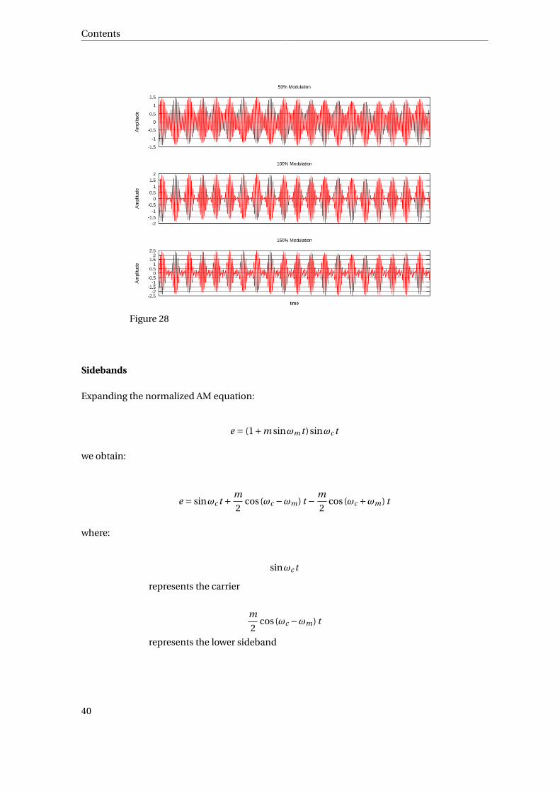
Contents

Figure 28

Sidebands

Expanding the normalized AM equation:

e = (1+m sinωm t )sinωc t

we obtain:

e = sinωc t + m

2cos(ωc −ωm) t − m

2cos(ωc +ωm) t

where:

sinωc t

represents the carrier

m

2cos(ωc −ωm) t

represents the lower sideband

40

Amplitude Modulation

m

2cos(ωc +ωm) t

represents the upper sideband

The sidebands are centered on the carrier frequency. The are the sum and difference frequenciesof the carrier and modulation signals. In the above example, they are just single frequencies, butnormally the baseband modulation signal is a range of frequencies and hence two bands areformed.

As a side point, note that multiplication in the time domain causes addition and subtraction inthe frequency domain.

0.58.2 AM Modulator

The standard amplitude modulation equation is:

eam = (1+m sinωm t )sinωc t

From this we notice that AM involves a multiplication process. (Recall that multiplication in thetime domain is equal to addition and subtraction in the frequency domain). There are severalways to perform this function electronically. The simplest method uses a switch.

Switching Modulators

Switching modulators can be placed into two categories: unipolar and bipolar.

Bipolar Switching Modulator

The bipolar switch is the easiest to visualize. Note that an AM waveform appears to consist of alow frequency dc signal whose polarity is reversing at a carrier rate.

41

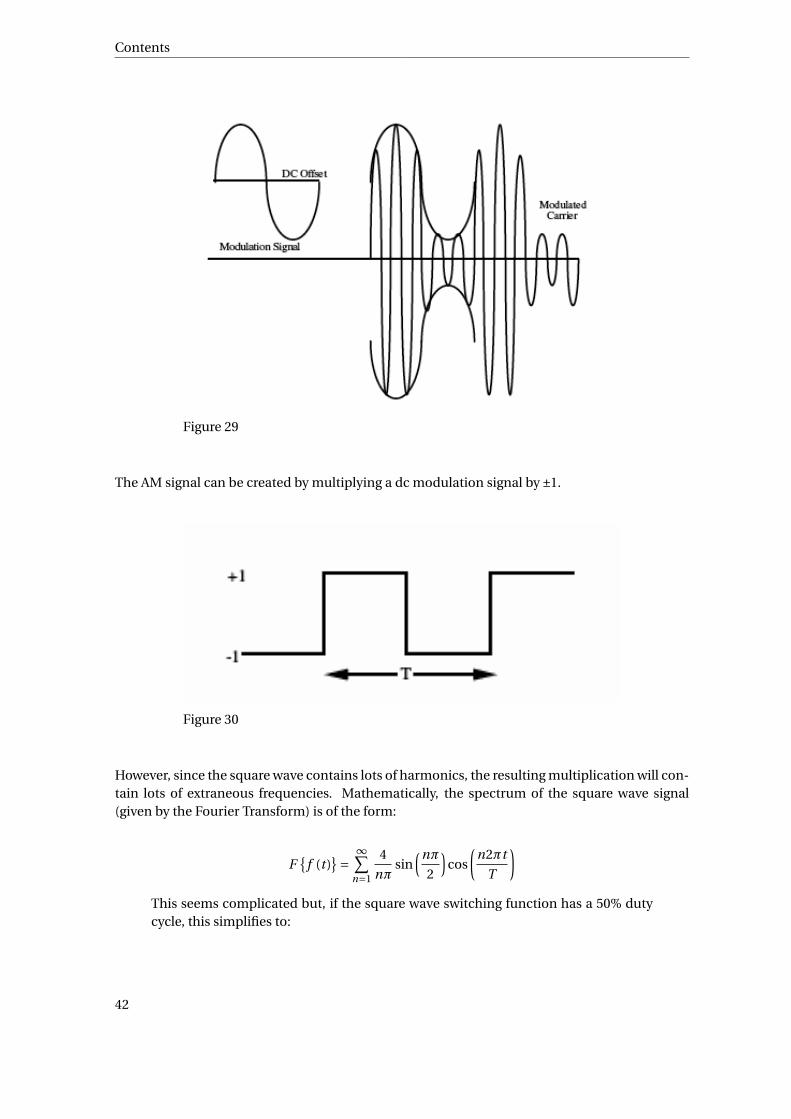
Contents

Figure 29

The AM signal can be created by multiplying a dc modulation signal by ±1.

Figure 30

However, since the square wave contains lots of harmonics, the resulting multiplication will con-tain lots of extraneous frequencies. Mathematically, the spectrum of the square wave signal(given by the Fourier Transform) is of the form:

F

f (t )= ∞∑

n=1

4

nπsin

(nπ

2

)cos

(n2πt

T

)This seems complicated but, if the square wave switching function has a 50% dutycycle, this simplifies to:

42

Amplitude Modulation

F

f (t )= 4

π

∞∑n=1,3,5...

1

ncos

(n2πt

T

)This tells us that the square wave is actually composed of a series of cosines (phaseshifted sines) at odd multiples of the fundamental switching frequency. Therefore,using this signal to multiply the baseband signal results in AM signals being gener-ated at each of the odd harmonics of the switching (carrier) frequencies. Since theamplitude of the harmonics decreases rapidly, this technique is practical for onlythe first few harmonics, and produces an enormous amount of unwanted signals(noise).

Figure 31

A band pass filter can be used to select any one of the AM signals. The number ofdifferent output frequencies can be significantly reduced if the multiplier acceptssinewaves at the carrier input.

DOUBLE-SIDEBAND SUPPRESSED-CARRIER TRANSMISSION27

Removing the DC component from the input eliminates the carrier signal and cre-ates DSBSC modulation.

Physically this is done by reversing the signal leads:

Figure 32

27 HTTP://EN.WIKIPEDIA.ORG/WIKI/DOUBLE-SIDEBAND%20SUPPRESSED-CARRIER%20TRANSMISSION

43

Contents

The process of reversing the polarity of a signal is easily accomplished by placing two switch pairsin the output of a differential amplifier. The MC1496 BALANCED MODULATOR28 is an exampleof such a device.

Figure 33

Unipolar Switching Modulator

As previously mentioned, an AM signal can be created by multiplying a dc modulation signal by0 & 1.

28 HTTP://WWW.ONSEMI.COM/PUB_LINK/COLLATERAL/MC1496-D.PDF

44

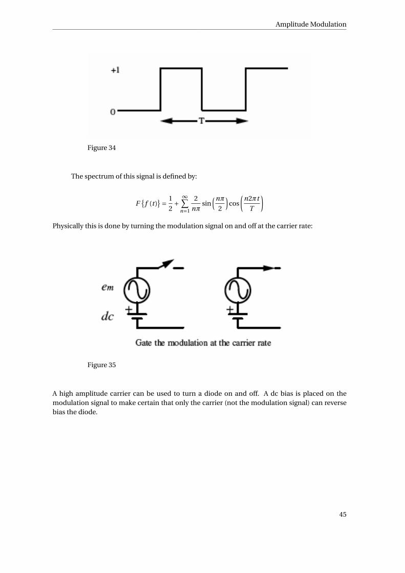
Amplitude Modulation

Figure 34

The spectrum of this signal is defined by:

F

f (t )= 1

2+

∞∑n=1

2

nπsin

(nπ

2

)cos

(n2πt

T

)

Physically this is done by turning the modulation signal on and off at the carrier rate:

Figure 35

A high amplitude carrier can be used to turn a diode on and off. A dc bias is placed on themodulation signal to make certain that only the carrier (not the modulation signal) can reversebias the diode.

45

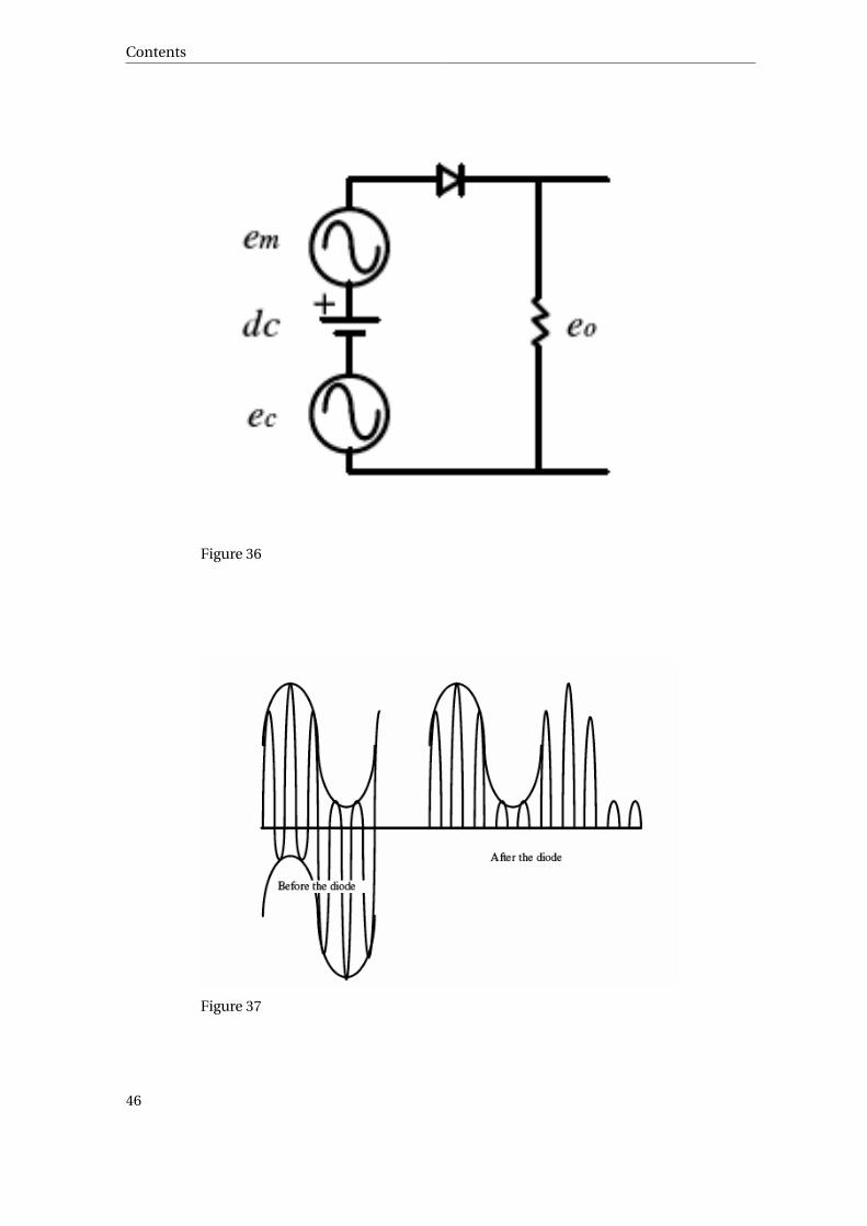
Contents

Figure 36

Figure 37

46

Amplitude Modulation

It may not seem obvious, but the output of this circuit contains a series of AM signals. A band-pass filter is needed to extract the desired one. Normally it is the 1st or 3rd harmonic of thefundamental. (The 1st harmonic is the fundamental.)

Collector Modulator

The diode switching modulator is incapable of producing high power signals since it is a passivedevice. A transistor can be used to overcome this limitation. A collector modulator is used forhigh level modulation.

Figure 38

Square Law Modulator

The voltage-current relationship of a diode is nonlinear near the knee and is of the form:

47

Contents

i (t ) = av (t )+bv2 (t )

The coefficient a and b are constants associated with the particular diode.

Figure 39

Amplitude modulation occurs if the diode is kept in the square law region when signals combine.

Figure 40

48

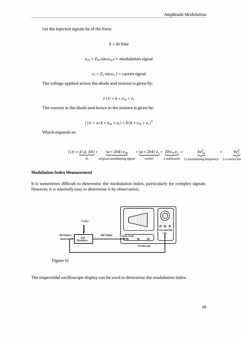
Amplitude Modulation

Let the injected signals be of the form:

k = dc bias

em = Em sinωm t = modulation signal

ec = Ec sinωc t = carrier signal

The voltage applied across the diode and resistor is given by:

v (t ) = k +em +ec

The current in the diode and hence in the resistor is given by:

i (t ) = a (k +em +ec )+b (k +em +ec )2

Which expands to:

i (t ) = k (a_bk)︸ ︷︷ ︸dc

+ (a +2bk)em︸ ︷︷ ︸original modulating signal

+ (a +2bk)ec︸ ︷︷ ︸carrier

+ 2bemec︸ ︷︷ ︸2 sidebands

+ be2m︸︷︷︸

2 x modulating frequency

+ be2c︸︷︷︸

2 x carrier frequency

Modulation Index Measurement

It is sometimes difficult to determine the modulation index, particularly for complex signals.However, it is relatively easy to determine it by observation.

Figure 41

The trapezoidal oscilloscope display can be used to determine the modulation index.

49

Contents

Figure 42

AM modulation index:

m = Emax −Emin

Emax +Emin

The trapezoidal display makes it possible to quickly recognize certain types of problems, whichwould reduce the AM signal quality.

Figure 43

The highest authorized carrier power for AM broadcast in the US is 50 kilowatts, although direc-tional stations are permitted 52.65 kilowatts to compensate for losses in the phasing system. TheERP can be much higher

C-QUAM

The basic idea behind the C-Quam modulator is actually quite simple. The output stage is anordinary AM modulator however; the carrier signal has been replaced by an amplitude limitedvector modulator. Therefore, the limiter output is really a phase-modulated signal.

50

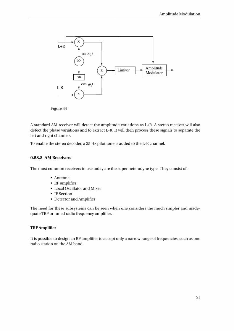
Amplitude Modulation

Figure 44

A standard AM receiver will detect the amplitude variations as L+R. A stereo receiver will alsodetect the phase variations and to extract L-R. It will then process these signals to separate theleft and right channels.

To enable the stereo decoder, a 25 Hz pilot tone is added to the L-R channel.

0.58.3 AM Receivers

The most common receivers in use today are the super heterodyne type. They consist of:

• Antenna• RF amplifier• Local Oscillator and Mixer• IF Section• Detector and Amplifier

The need for these subsystems can be seen when one considers the much simpler and inade-quate TRF or tuned radio frequency amplifier.

TRF Amplifier

It is possible to design an RF amplifier to accept only a narrow range of frequencies, such as oneradio station on the AM band.

51

Contents

Figure 45

By adjusting the center frequency of the tuned circuit, all other input signals can be excluded.

Figure 46

The AM band ranges from about 500 kHz to 1600 kHz. Each station requires 10 kHz of this spec-trum, although the baseband signal is only 5 kHz.

Recall that for a tuned circuit: Q = fc

B . The center or resonant frequency in an RLC networkis most often adjusted by varying the capacitor value. However, the Q remains approximatelyconstant as the center frequency is adjusted. This suggests that as the bandwidth varies as thecircuit is tuned.

For example, the Q required at the lower end of the AM band to select only one radiostation would be approximately:

Q = fc

B= 500 kH z

10 kH z= 50

52

Amplitude Modulation

As the tuned circuit is adjusted to the higher end of the AM band, the resulting band-width is:

B = fc

Q= 1600 kH z

50= 30 kH z

A bandwidth this high could conceivably pass three adjacent stations, thus making meaningfulreception impossible.

To prevent this, the incoming RF signal is heterodyned to a fixed IF or intermediate frequencyand passed through a constant bandwidth circuit.

Superheterodyne Receiver

Figure 47

The RF amplifier boosts the RF signal into the mixer. It has broad tuning and amplifies not justone RF station, but many of them simultaneously. It also amplifies any input noise and evencontributes some of its own.

The other mixer input is a high frequency sine wave created by a local oscillator. In AM receivers,it is always 455 kHz above the desired station carrier frequency. An ideal mixer will combine theincoming carrier with the local oscillator to create sum and difference frequencies. .

A real mixer combines two signals and creates a host of new frequencies:

• A dc level• The original two frequencies• The sum and difference of the two input frequencies• Harmonics of the two input frequencies• Sums and differences of all of the harmonics

Since the RF amplifier passes several radio stations at once, the mixer output can be very com-plex. However, the only signal of real interest is the difference between the desired station carrierfrequency and the local oscillator frequency. This difference frequency, also called the IF (inter-mediate frequency) will alway be 455 kHz. By passing this through a 10 kHz BPF (band pass filter)centered at 455 kHz, the bulk of the unwanted signals can be eliminated.

53

Contents

Local Oscillator Frequency

Since the mixer generates sum and difference frequencies, it is possible to generate the 455 kHzIF signal if the local oscillator is either above or below the IF. The inevitable question is which ispreferable.

Case I The local Oscillator is above the IF. This would require that theoscillator tune from (500 + 455) kHz to (1600 + 455) kHz or approximately1 to 2 MHz. It is normally the capacitor in a tuned RLC circuit, which isvaried to adjust the center frequency while the inductor is left fixed.

Since

fc = 1

2πp

LC

solving for C we obtain

C = 1

L(2π fc

)2

When the tuning frequency is a maximum, the tuning capacitor is a min-imum and vice versa. Since we know the range of frequencies to be cre-ated, we can deduce the range of capacitance required.

Cmax

Cmin= L

(2π fmax

)2

L(2π fmin

)2 =(

2 M H z

1 M H z

)2

= 4

Making a capacitor with a 4:1 value change is well within the realm of possibility.

Case II The local Oscillator is below the IF. This would require that theoscillator tune from (500 - 455) kHz to (1600 - 455) kHz or approximately45 kHz to 1145 kHz, in which case:

Cmax

Cmin=

(1145 kH z

45 kH z

)2

≈ 648

It is not practical to make a tunable capacitor with this type of range. Therefore the local oscilla-tor in a standard AM receiver is above the radio band.

Image Frequency

Just as there are two oscillator frequencies, which can create the same IF, two different stationfrequencies can create the IF. The undesired station frequency is known as the image frequency.

54

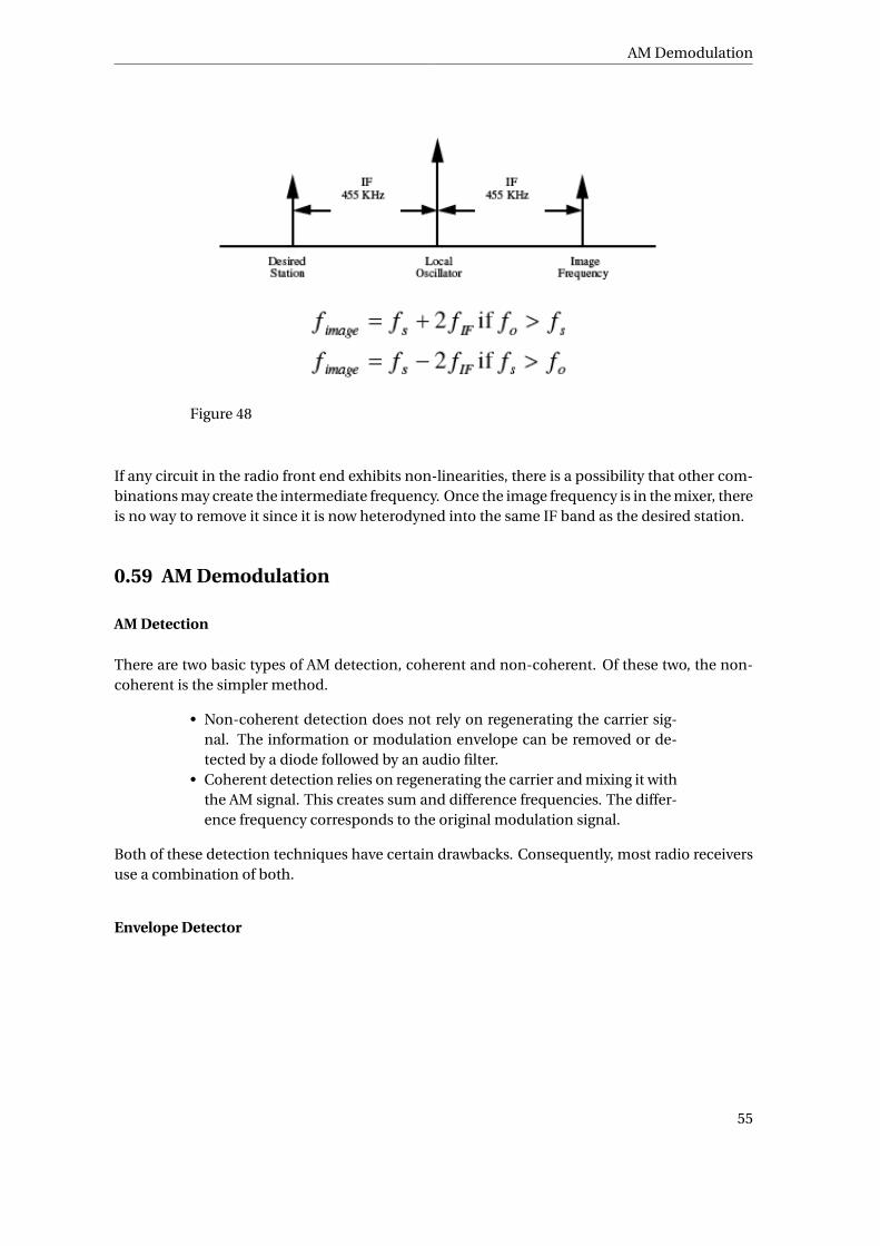
AM Demodulation

Figure 48

If any circuit in the radio front end exhibits non-linearities, there is a possibility that other com-binations may create the intermediate frequency. Once the image frequency is in the mixer, thereis no way to remove it since it is now heterodyned into the same IF band as the desired station.

0.59 AM Demodulation

AM Detection

There are two basic types of AM detection, coherent and non-coherent. Of these two, the non-coherent is the simpler method.

• Non-coherent detection does not rely on regenerating the carrier sig-nal. The information or modulation envelope can be removed or de-tected by a diode followed by an audio filter.

• Coherent detection relies on regenerating the carrier and mixing it withthe AM signal. This creates sum and difference frequencies. The differ-ence frequency corresponds to the original modulation signal.

Both of these detection techniques have certain drawbacks. Consequently, most radio receiversuse a combination of both.

Envelope Detector

55

Contents

Figure 49

When trying to demodulate an AM signal, it seems like good sense that only the amplitude of thesignal needs to be examined. By only examining the amplitude of the signal at any given time, wecan remove the carrier signal from our considerations, and we can examine the original signal.Luckily, we have a tool in our toolbox that we can use to examine the amplitude of a signal: TheEnvelope Detector.

An envelope detector is simply a half wave rectifier followed by a low pass filter. In the case ofcommercial AM radio receivers, the detector is placed after the IF section. The carrier at thispoint is 455 kHz while the maximum envelope frequency is only 5 kHz. Since the ripple compo-nent is nearly 100 times the frequency of the highest baseband signal and does not pass throughany subsequent audio amplifiers.

An AM signal where the carrier frequency is only 10 times the envelope frequencywould have considerable ripple:

Figure 50

56

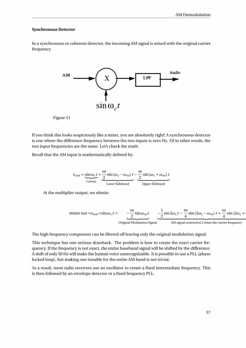
AM Demodulation

Synchronous Detector

In a synchronous or coherent detector, the incoming AM signal is mixed with the original carrierfrequency.

Figure 51

If you think this looks suspiciously like a mixer, you are absolutely right! A synchronous detectoris one where the difference frequency between the two inputs is zero Hz. Of in other words, thetwo input frequencies are the same. Let’s check the math.

Recall that the AM input is mathematically defined by:

eam = sinωc t︸ ︷︷ ︸Carrier

+ m

2sin(ωc −ωm) t︸ ︷︷ ︸

Lower Sideband

− m

2sin(ωc +ωm) t︸ ︷︷ ︸

Upper Sideband

At the multiplier output, we obtain:

mixer out =eam×sinωc t = −m

2sinωm t︸ ︷︷ ︸

Original Modulation Signal

−1

2sin2ωc t − m

4sin(2ωc −ωm) t + m

4sin(2ωc +ωm) t︸ ︷︷ ︸

AM signal centered at 2 times the carrier frequency

The high frequency component can be filtered off leaving only the original modulation signal.

This technique has one serious drawback. The problem is how to create the exact carrier fre-quency. If the frequency is not exact, the entire baseband signal will be shifted by the difference.A shift of only 50 Hz will make the human voice unrecognizable. It is possible to use a PLL (phaselocked loop), but making one tunable for the entire AM band is not trivial.

As a result, most radio receivers use an oscillator to create a fixed intermediate frequency. Thisis then followed by an envelope detector or a fixed frequency PLL.

57

Contents

Squaring Detector

The squaring detector is also a synchronous or coherent detector. It avoids the problem of havingto recreate the carrier by simply squaring the input signal. It essentially uses the AM signal itselfas a sort of wideband carrier.

Figure 52

The output of the multiplier is the square of the input AM signal:

(eam)2 =(sinωc t + m

2cos(ωc −ωm) t − m

2cos(ωc +ωm) t

)2

Since the input is being multiplied by the sinωc t component, one of the resulting differenceterms is the original modulation signal. The principle difficulty with this approach is trying tocreate a linear, high frequency multiplier.

0.60 AM-DSBSC

AM-DSB-SC is characterized by the following transmission equation:

v(t ) = As(t )cos(2π fc t )

It is important to notice that s(t) can contain a negative value. AM-DSB-SC requires a coher-ent receiver, because the modulation data can go negative, and therefore the receiver needs toknow that the signal is negative (and not just phase shifted). AM-DSB-SC systems are very sus-ceptible to frequency shifting and phase shifting on the receiving end. In this equation, A is thetransmission amplitude.

Double side band suppressed carrier modulation is simply AM without the broadcast carrier.Recall that the AM signal is defined by:

58

AM-DSBSC

eam = (1+m sinωm t )sinωc t = sinωc t+m2

2cos(ωc −ωm) t−m2

2cos(ωc +ωm) t

The carrier term in the spectrum can be eliminated by removing the dc offset fromthe modulating signal:

eDSBSC = m sinωm t sinωc t = m2

2cos(ωc −ωm) t−m2

2cos(ωc +ωm) t

0.60.1 Double Balanced Ring Modulator

One of the circuits which is capable of creating DSBSC is the double balance ring modulator.

Figure 53

If the carrier is large enough to cause the diodes to switch states, then the circuit acts like a diodeswitching modulator:

Figure 54

59

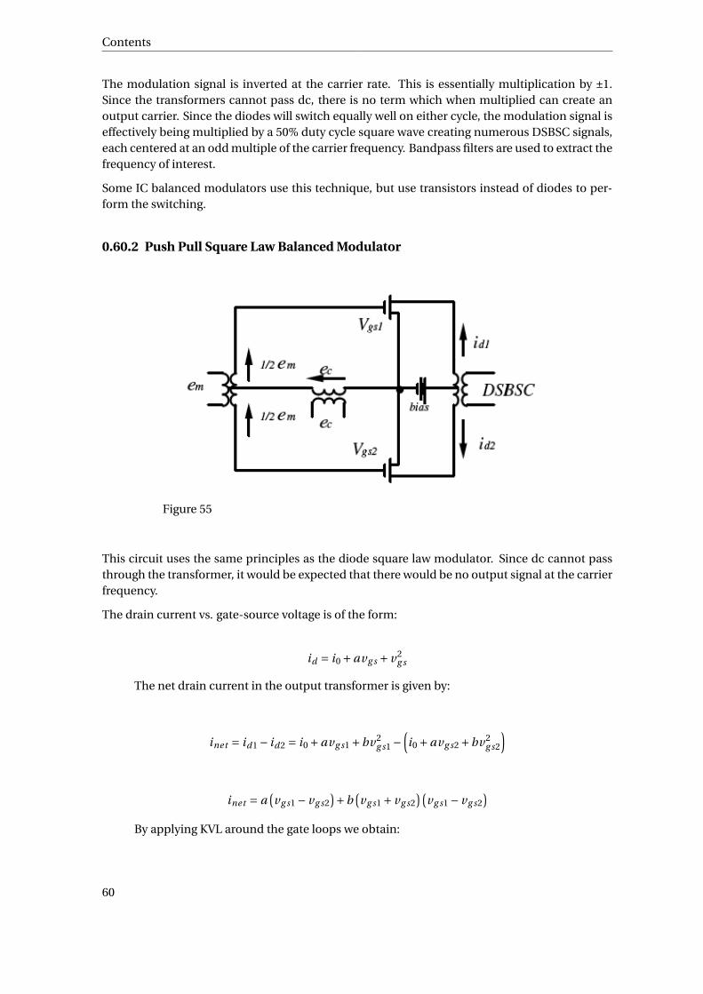
Contents

The modulation signal is inverted at the carrier rate. This is essentially multiplication by ±1.Since the transformers cannot pass dc, there is no term which when multiplied can create anoutput carrier. Since the diodes will switch equally well on either cycle, the modulation signal iseffectively being multiplied by a 50% duty cycle square wave creating numerous DSBSC signals,each centered at an odd multiple of the carrier frequency. Bandpass filters are used to extract thefrequency of interest.

Some IC balanced modulators use this technique, but use transistors instead of diodes to per-form the switching.

0.60.2 Push Pull Square Law Balanced Modulator

Figure 55

This circuit uses the same principles as the diode square law modulator. Since dc cannot passthrough the transformer, it would be expected that there would be no output signal at the carrierfrequency.

The drain current vs. gate-source voltage is of the form:

id = i0 +avg s + v2g s

The net drain current in the output transformer is given by:

inet = id1 − id2 = i0 +avg s1 +bv2g s1 −

(i0 +avg s2 +bv2

g s2

)

inet = a(vg s1 − vg s2

)+b(vg s1 + vg s2

)(vg s1 − vg s2

)By applying KVL around the gate loops we obtain:

60

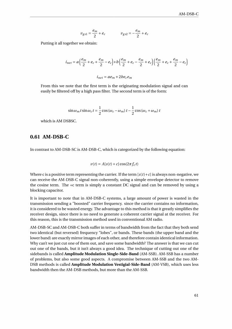
AM-DSB-C

vg s1 = em

2+ec vg s2 =−em

2+ec

Putting it all together we obtain:

inet = a(em

2+ec + em

2−ec

)+b

(em

2+ec − em

2+ec

)(em

2+ec + em

2−ec

)

inet = aem +2bec em

From this we note that the first term is the originating modulation signal and caneasily be filtered off by a high pass filter. The second term is of the form:

sinωm t sinωc t = 1

2cos(ωc −ωm) t − 1

2cos(ωc +ωm) t

which is AM DSBSC.

0.61 AM-DSB-C

In contrast to AM-DSB-SC is AM-DSB-C, which is categorized by the following equation:

v(t ) = A[s(t )+ c]cos(2π fc t )

Where c is a positive term representing the carrier. If the term [s(t )+c] is always non-negative, wecan receive the AM-DSB-C signal non-coherently, using a simple envelope detector to removethe cosine term. The +c term is simply a constant DC signal and can be removed by using ablocking capacitor.

It is important to note that in AM-DSB-C systems, a large amount of power is wasted in thetransmission sending a "boosted" carrier frequency. since the carrier contains no information,it is considered to be wasted energy. The advantage to this method is that it greatly simplifies thereceiver design, since there is no need to generate a coherent carrier signal at the receiver. Forthis reason, this is the transmission method used in conventional AM radio.

AM-DSB-SC and AM-DSB-C both suffer in terms of bandwidth from the fact that they both sendtwo identical (but reversed) frequency "lobes", or bands. These bands (the upper band and thelower band) are exactly mirror images of each other, and therefore contain identical information.Why can’t we just cut one of them out, and save some bandwidth? The answer is that we can cutout one of the bands, but it isn’t always a good idea. The technique of cutting out one of thesidebands is called Amplitude Modulation Single-Side-Band (AM-SSB). AM-SSB has a numberof problems, but also some good aspects. A compromise between AM-SSB and the two AM-DSB methods is called Amplitude Modulation Vestigial-Side-Band (AM-VSB), which uses lessbandwidth then the AM-DSB methods, but more than the AM-SSB.

61

Contents

0.61.1 Transmitter

A typical AM-DSB-C transmitter looks like this:

c cos(...)| |

Signal ---->(+)---->(X)----> AM-DSB-C

which is a little more complicated than an AM-DSB-SC transmitter.

0.61.2 Receiver

An AM-DSB-C receiver is very simple:

AM-DSB-C ---->|Envelope Filter|---->|Capacitor|----> Signal

The capacitor blocks the DC component, and effectively removes the +c term.

0.62 AM-SSB

To send an AM-SSB signal, we need to remove one of the sidebands from an AM-DSB signal. Thismeans that we need to pass the AM-DSB signal through a filter, to remove one of the sidebands.The filter, however, needs to be a very high order filter, because we need to have a very aggres-sive roll-off. One sideband needs to pass the filter almost completely unchanged, and the othersideband needs to be stopped completely at the filter.

To demodulate an AM-SSB signal, we need to perform the following steps:

1. Low-pass filter, to remove noise2. Modulate the signal again by the carrier frequency3. Pass through another filter, to remove high-frequency components4. Amplify the signal, because the previous steps have attenuated it significantly.

AM-SSB is most efficient in terms of bandwidth, but there is a significant added cost involved interms of more complicated hardware to send and receive this signal. For this reason, AM-SSB israrely seen as being cost effective.

Single sideband is a form of AM with the carrier and one sideband removed. In normal AMbroadcast, the transmitter is rated in terms of the carrier power. SSB transmitters attempt toeliminate the carrier and one of the sidebands. Therefore, transmitters are rated in PEP (peakenvelope power).

PEP =(peak envelope voltage

)2

2RL

With normal voice signals, an SSB transmitter outputs 1/4 to 1/3 PEP.

62

AM-SSB

There a numerous variations of SSB:

• SSB - Single sideband - amateur radio• SSSC - Single sideband suppressed carrier - a small pilot carrier is trans-

mitted• ISB - Independent sideband - two separate sidebands with a sup-

pressed carrier. Used in radio telephony.• VSB - Vestigial sideband - a partial sideband. Used in broadcast TV.• ACSSB - Amplitude companded SSB

There are several advantages of using SSB:

• More efficient spectrum utilization• Less subject to selective fading• More power can be placed in the intelligence signal• 10 to 12 dB noise reduction due to bandwidth limiting

0.62.1 Filter Method

The simplest way to create SSB is to generate DSBSC and then use a bandpass filter to extractone of the sidebands.

Figure 56

This technique can be used at relatively low carrier frequencies. At high frequencies, the Q of thefilter becomes unacceptably high. The required Q necessary to filter off one of the sidebands canbe approximated by:

Q ≈ fcp

S

4∆ f

where:

fc = carrier frequency

∆ f = sideband separation

63

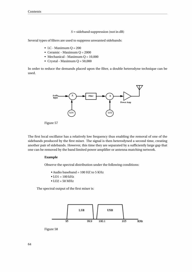
Contents

S = sideband suppression (not in dB)

Several types of filters are used to suppress unwanted sidebands:

• LC - Maximum Q = 200• Ceramic - Maximum Q = 2000• Mechanical - Maximum Q = 10,000• Crystal - Maximum Q = 50,000

In order to reduce the demands placed upon the filter, a double heterodyne technique can beused.

Figure 57

The first local oscillator has a relatively low frequency thus enabling the removal of one of thesidebands produced by the first mixer. The signal is then heterodyned a second time, creatinganother pair of sidebands. However, this time they are separated by a sufficiently large gap thatone can be removed by the band limited power amplifier or antenna matching network.

Example

Observe the spectral distribution under the following conditions:

• Audio baseband = 100 HZ to 5 KHz• LO1 = 100 kHz• LO2 = 50 MHz

The spectral output of the first mixer is:

Figure 58

64

AM-SSB

If the desired sideband suppression is 80 dB, the Q required to filter offone of the sidebands is approximately:

S = log−1(

80

20

)= 104

Q ≈ fcp

S

4∆ f= 100×103

p104

4×200= 12500

It is evident that a crystal filter would be needed to remove the unwanted sideband.

After the filter, only one sideband is left. In this example, we’ll retain the USB. Thespectrum after the second mixer is:

Figure 59

The Q required to suppress one of the side bands by 80 dB is approximately:

Q ≈ fcp

S

4∆ f= 50×106

p104

4×200.2×103 = 6244

Thus, we note that the required Q drops in half.

This SSB filter technique is used in radiotelephone applications.

65

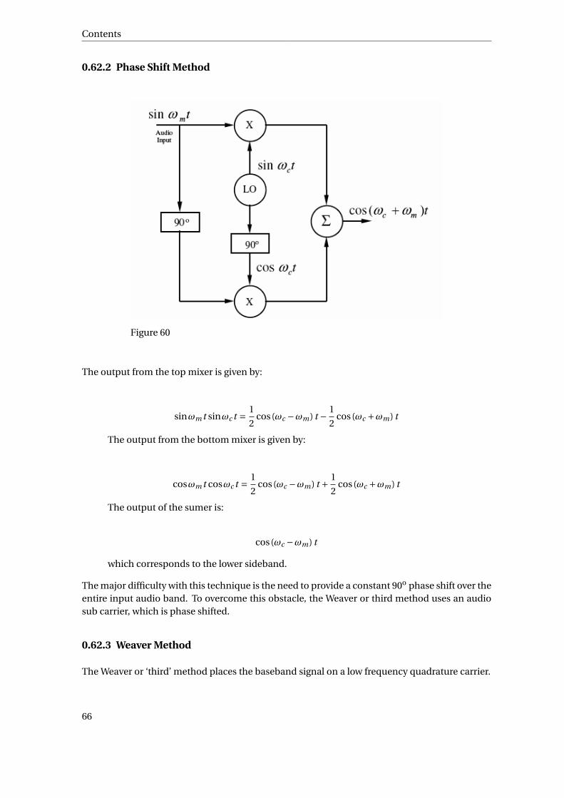
Contents

0.62.2 Phase Shift Method

Figure 60

The output from the top mixer is given by:

sinωm t sinωc t = 1

2cos(ωc −ωm) t − 1

2cos(ωc +ωm) t

The output from the bottom mixer is given by:

cosωm t cosωc t = 1

2cos(ωc −ωm) t + 1

2cos(ωc +ωm) t

The output of the sumer is:

cos(ωc −ωm) t

which corresponds to the lower sideband.

The major difficulty with this technique is the need to provide a constant 90o phase shift over theentire input audio band. To overcome this obstacle, the Weaver or third method uses an audiosub carrier, which is phase shifted.

0.62.3 Weaver Method

The Weaver or ‘third’ method places the baseband signal on a low frequency quadrature carrier.

66

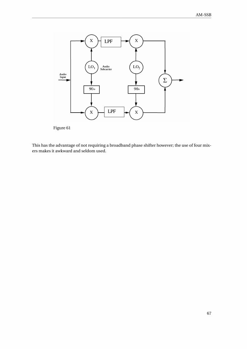
AM-SSB

Figure 61

This has the advantage of not requiring a broadband phase shifter however; the use of four mix-ers makes it awkward and seldom used.

67

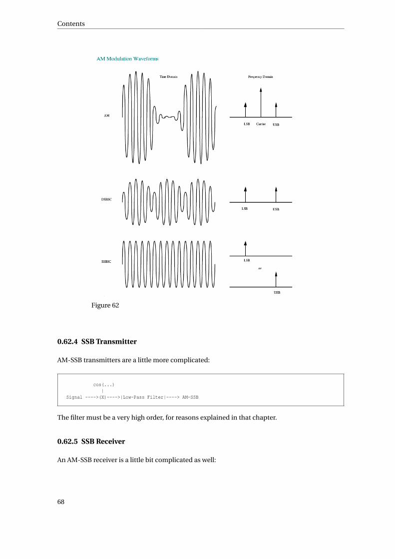
Contents

Figure 62

0.62.4 SSB Transmitter

AM-SSB transmitters are a little more complicated:

cos(...)|

Signal ---->(X)---->|Low-Pass Filter|----> AM-SSB

The filter must be a very high order, for reasons explained in that chapter.

0.62.5 SSB Receiver

An AM-SSB receiver is a little bit complicated as well:

68

AM-VSB

cos(...)|

AM-SSB ---->(X)---->|Low-Pass Filter|---->|Amplifier|----> Signal

This filter doesnt need to be a very high order, like the transmitter has.

These receivers require extremely stable oscillators, good adjacent channel selectivity, and typi-cally use a double conversion technique. Envelope detectors cannot be used since the envelopevaries at twice the frequency of the AM envelope.

Stable oscillators are needed since the detected signal is proportional to the difference betweenthe untransmitted carrier and the instantaneous side band. A small shift of 50 Hz makes thereceived signal unusable.

SSB receivers typically use fixed frequency tuning rather than continuous tuning as found onmost radios. Crystal oscillators are often used to select the fixed frequency channels.

0.63 AM-VSB

As a compromise between AM-SSB and AM-DSB is AM-VSB. To make an AM-VSB signal, we passan AM-DSB signal through a lowpass filter. Now, the trick is that we pass it through a low-orderfilter, so that some of the filtered sideband still exists. This filtered part of the sideband is calledthe "Vestige" of the sideband, hence the name "Vestigial Side Band".

AM-VSB signals then can get demodulated in a similar manner to AM-SSB. We can see when weremodulate the input signal, the two vestiges (the positive and negative mirrors of each other)over-lap each other, and add up to the original, unfiltered value!

AM-VSB is less expensive to implement then AM-SSB because we can use lower-order filters.

i Information

Broadcast television in North America uses AM-VSB

0.63.1 Transmitter

here we will talk about an AM-VSB transmitter circuit.

0.63.2 Receiver

here we will talk about an AM-VSB receiver circuit. (AM)

69

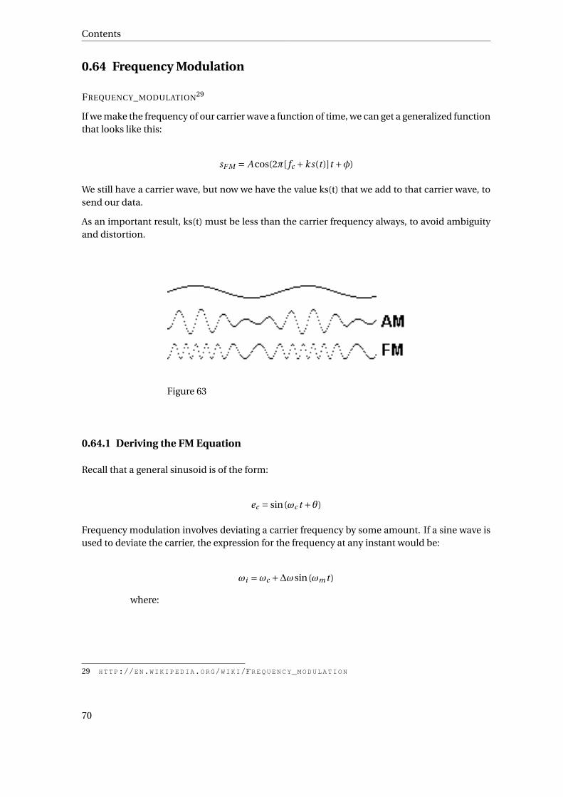
Contents

0.64 Frequency Modulation

FREQUENCY_MODULATION29

If we make the frequency of our carrier wave a function of time, we can get a generalized functionthat looks like this:

sF M = A cos(2π[ fc +ks(t )]t +φ)

We still have a carrier wave, but now we have the value ks(t) that we add to that carrier wave, tosend our data.

As an important result, ks(t) must be less than the carrier frequency always, to avoid ambiguityand distortion.

Figure 63

0.64.1 Deriving the FM Equation

Recall that a general sinusoid is of the form:

ec = sin(ωc t +θ)

Frequency modulation involves deviating a carrier frequency by some amount. If a sine wave isused to deviate the carrier, the expression for the frequency at any instant would be:

ωi =ωc +∆ωsin(ωm t )

where:

29 HTTP://EN.WIKIPEDIA.ORG/WIKI/FREQUENCY_MODULATION

70

Frequency Modulation

ωi =instantaneous frequency

ωc =carrier frequency

∆ω=carrier deviation

ωm =modulation frequency

This expression describes a signal varying sinusoidally about some average frequency. However,we cannot simply substitute this expression into the general equation for a sinusoid to get theFM equation. This is because the sine operator acts on angles, not frequency. Therefore, we mustdefine the instantaneous frequency in terms of angles.

It should be noted that the modulation signal amplitude governs the amount of carrier deviationwhile the modulation signal frequency governs the rate of carrier deviation.

The term ω is an angular velocity (radians per second) and is related to frequency and angle bythe following relationship:

ω= 2πf =dθ

d t

To find the angle, we must integrateω

with respect to time:

∫ωd t = θ

We can now find the instantaneous angle associated with the instantaneous fre-quency:

θ = ∫ωi d t = ∫

(ωc +∆ωsin(ωm t ))d t =ωc t − ∆ωωm

cos(ωm t ) =ωc t − ∆ ffm

cos(ωm t )

This angle can now be substituted into the general carrier signal to define FM:

e f m = sin

(ωc t − ∆ f

fmcos(ωm t )

)The FM modulation index is defined as the ratio of the carrier deviation to modula-tion frequency:

71

Contents

m f m = ∆ f

fm

Consequently, the FM equation is often written as:

e f m = sin(ωc t −m f m cos(ωm t )

)0.64.2 Bessel’s Functions

BESSEL_FUNCTION30

This is a very complex expression and it is not readily apparent what the sidebands of this signalare like. The solution to this problem requires a knowledge of Bessel’s functions of the first kindand order p. In open form, it resembles:

Jp (x) =∞∑

k=0

(−1)k( x

2

)2k+p

k !(k +p

)!

where:

Jp (x) =Magnitude of the frequency component

p =Side frequency number (not to be confused with side-bands)

x =Modulation index

As a point of interest, Bessel’s functions are a solution to the following equation:

x2 + d 2 y

d x2 +xd y

d x+ (

x2 −p2)= 0

Bessel’s functions occur in the theory of cylindrical and spherical waves, much like sine wavesoccur in the theory of plane waves.

It turns out that FM generates an infinite number of side frequencies (in both the upper andlower sidebands). Each side frequency is an integer multiple of the modulation signal frequency.The amplitude of higher order side frequencies decreases rapidly and can generally be ignored.

30 HTTP://EN.WIKIPEDIA.ORG/WIKI/BESSEL_FUNCTION

72

Frequency Modulation

The amplitude of the carrier signal is also a function of the modulation index and under someconditions, its amplitude can actually go to zero. This does not mean that the signal disappears,but rather that all of the broadcast energy is redistributed to the side frequencies.

A plot of the carrier and first five side frequency amplitudes as a function of modulation indexresembles:

Figure 64

The Bessel coefficients have several interesting properties including:

J 20 +2

(J 2

1 + J 22 + J 2

3 +·· ·)= 1

One very useful interpretation of this is: J0 represents the voltage amplitude of the carrier, J1

represents the amplitude of the 1st side frequency, J2 the 2nd side frequency etc. Note that thesum of the squares (power) remains constant.

0.64.3 FM Bandwidth

FM generates upper and lower sidebands, each of which contain an infinite number of side fre-quencies. However, the FM bandwidth is not infinite because the amplitude of the higher orderside frequencies decreases rapidly. Carson’s Rule is often used to calculate the bandwidth, sinceit contains more than 90% of the FM signal.

Carson’s Rule

CARSON%27S_RULE31

B f m ≈ 2(m f m +1

)fm = 2

(∆ f + fm

))

31 HTTP://EN.WIKIPEDIA.ORG/WIKI/%20CARSON%2527S_RULE

73

Contents

In commercial broadcast applications, the maximum modulation index (m f m) = 5, the maxi-mum, carrier deviation (∆ f ) = 75 kHz, and maximum modulation frequency ( fm) = 15 kHz. Thetotal broadcast spectrum according to Carson’s rule is 180 kHz, but an additional 20 kHz guardband is used to separate adjacent radio stations. Therefore, each FM radio station is allocated200 kHz.

0.64.4 Noise

In AM systems, noise easily distorts the transmitted signal however, in FM systems any addednoise must create a frequency deviation in order to be perceptible.

Figure 65

The maximum frequency deviation due to random noise occurs when the noise is at right anglesto the resultant signal. In the worst case the signal frequency has been deviated by:

δ= θ fm

This shows that the deviation due to noise increases as the modulation frequency increases.Since noise power is the square of the noise voltage, the signal to noise ratio can significantlydegrade.

Figure 66

74

Frequency Modulation

To prevent this, the amplitude of the modulation signal is increased to keep the S/N ratio con-stant over the entire broadcast band. This is called pre-emphasis.

0.64.5 Pre & De-emphasis

PREEMPHASIS32

Increasing the amplitude of high frequency baseband signals in the FM modulator (transmitter)must be compensated for in the FM demodulator (receiver) otherwise the signal would soundquite tinny (too much treble).

The standard curves resemble:

Figure 67

In commercial FM broadcast, the emphasis circuits consist of a simple RC network with a timeconstant of 75 µSec and a corner frequency of 2125 Hz.

Figure 68

32 HTTP://EN.WIKIPEDIA.ORG/WIKI/PREEMPHASIS

75

Contents

The magnitude of the pre-emphasis response is defined by:

Figure 69

0.65 FM Transmission Power

The equation for the transmitted power in a sinusoid is a fundamental equation. Remember it.

Since the value of the amplitude of the sine wave in FM does not change, the transmitted poweris a constant. As a general rule, for a sinusoid with a constant amplitude, the transmitted powercan be found as follows:

P (t ) = A2

2RL

Where A is the amplitude of the sine wave, and RL is the resistance of the load. In a normalizedsystem, we set RL to 1.

The Bessel coefficients can be used to determine the power in the carrier and any side frequency:

PT = PC(

J 20 +2

(J 2

1 + J 22 + J 2

3 +·· ·))

PC

is the power in the unmodulated carrier.

PT

is the total power and is by definition equal to the unmodulated carrierpower.

As the modulation index varies, the individual Bessel coefficients change and power is redis-tributed from the carrier to the side frequencies.

76

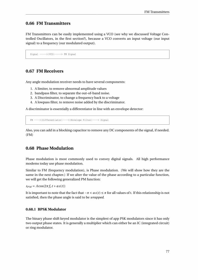
FM Transmitters

0.66 FM Transmitters

FM Transmitters can be easily implemented using a VCO (see why we discussed Voltage Con-trolled Oscillators, in the first section?), because a VCO converts an input voltage (our inputsignal) to a frequency (our modulated output).

Signal ----->|VCO|-----> FM Signal

0.67 FM Receivers

Any angle modulation receiver needs to have several components:

1. A limiter, to remove abnormal amplitude values2. bandpass filter, to separate the out-of-band noise.3. A Discriminator, to change a frequency back to a voltage4. A lowpass filter, to remove noise added by the discriminator.

A discriminator is essentially a differentiator in line with an envelope detector:

FM ---->|Differentiator|---->|Envelope Filter|----> Signal

Also, you can add in a blocking capacitor to remove any DC components of the signal, if needed.(FM)

0.68 Phase Modulation

Phase modulation is most commonly used to convey digital signals. All high performancemodems today use phase modulation.

Similar to FM (frequency modulation), is Phase modulation. (We will show how they are thesame in the next chapter.) If we alter the value of the phase according to a particular function,we will get the following generalized PM function:

sP M = A cos(2π fc t +αs(t ))

It is important to note that the fact that −π<αs(t ) ≤π for all values of t. If this relationship is notsatisfied, then the phase angle is said to be wrapped.

0.68.1 BPSK Modulator

The binary phase shift keyed modulator is the simplest of app PSK modulators since it has onlytwo output phase states. It is generally a multiplier which can either be an IC (integrated circuit)or ring modulator.

77

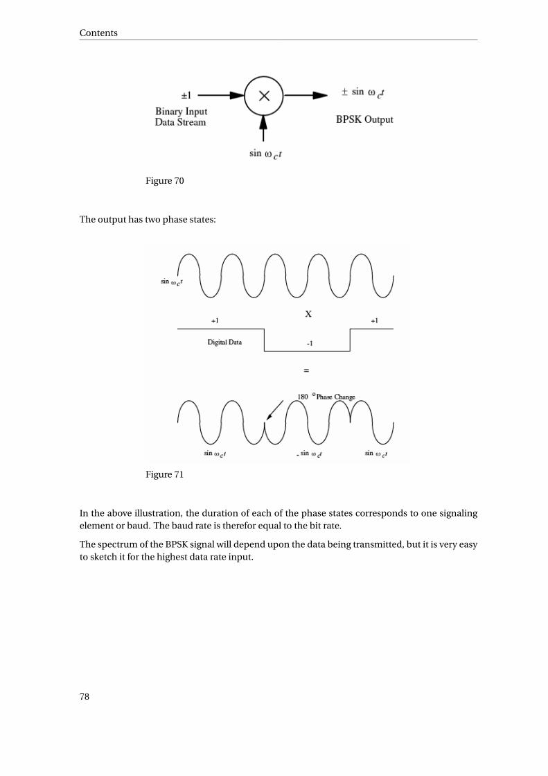
Contents

Figure 70

The output has two phase states:

Figure 71

In the above illustration, the duration of each of the phase states corresponds to one signalingelement or baud. The baud rate is therefor equal to the bit rate.

The spectrum of the BPSK signal will depend upon the data being transmitted, but it is very easyto sketch it for the highest data rate input.

78

Phase Modulation

Figure 72

The resultant BPSK spectrum is:

Figure 73

0.68.2 QPSK Modulators (4-PSK)

Quadrature modulation uses two data channels denoted I (in phase) and Q (quadrature phase)displaced by 90o with respect to each other. It may seem somewhat paradoxical, that althoughthese two channels are combined prior to transmission, they do not interfere with each other.

79

Contents

Figure 74

The receiver is quite capable of separating them because of their quadrature or orthogonal na-ture.

Figure 75

In the most basic configuration, there are 4 possible output phases. This suggests that eachoutput symbol correspond to 2 bits of binary information. Since several bits can be encodedinto a baud, the bit rate exceeds the baud rate.

80

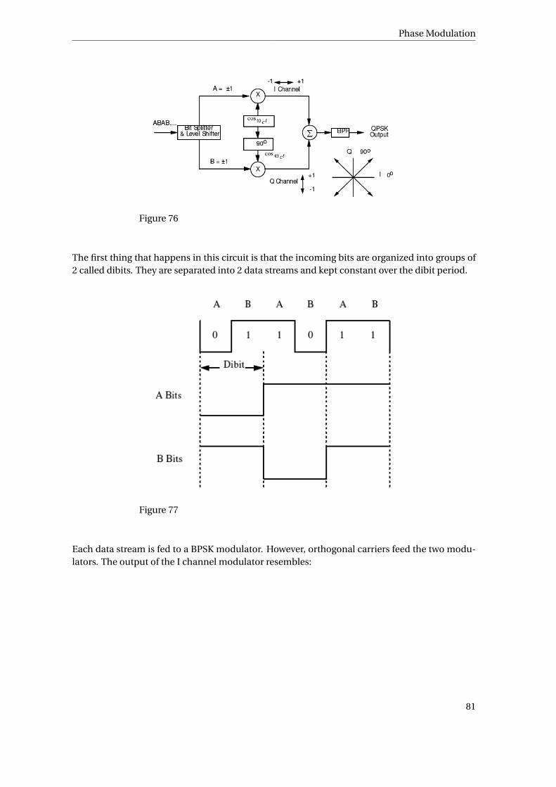
Phase Modulation

Figure 76

The first thing that happens in this circuit is that the incoming bits are organized into groups of2 called dibits. They are separated into 2 data streams and kept constant over the dibit period.

Figure 77

Each data stream is fed to a BPSK modulator. However, orthogonal carriers feed the two modu-lators. The output of the I channel modulator resembles:

81

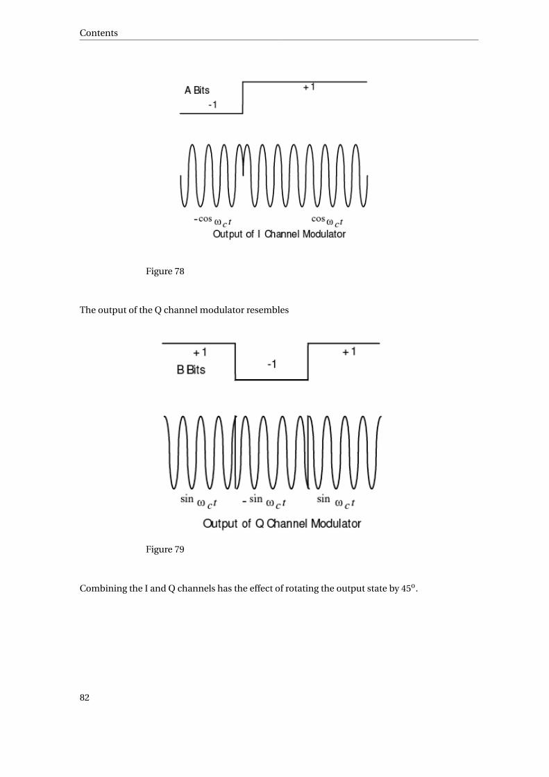
Contents

Figure 78

The output of the Q channel modulator resembles

Figure 79

Combining the I and Q channels has the effect of rotating the output state by 45o.

82

Phase Modulation

Figure 80

Rotating the output reference to 45o for the sake of clarity, the transmitted output for this partic-ular data sequence is therefor:

Figure 81

0.68.3 8-PSK

This process of encoding more bits into each output baud or phase state can be continued. Or-ganizing binary bits into 3 bytes corresponds to 8 different conditions.

The output constellation diagram for the 8 different phase states is:

83

Contents

Figure 82

From this diagram it is readily apparent that two different amplitudes are needed on the I andQ channels. If the A bit is used to control the polarity of the I channel and the B bit the polarityof the Q channel, then the C bit can be used to define the two different amplitudes. In order toevenly space the phase states; the amplitudes must be ± 0.38 and ± 0.92. The magnitude of the Iand Q channel signals must always be different. An inverter can be used to assure this condition.

The input bit stream is organized into 3 bit bytes. Each bit is sent to a different location to controla certain aspect of the modulator. The inputs to the 2 - 4 level converter are 0’s or 1’s but theoutput is ± 0.38 or ± 0.92, depending on the C bit.

Figure 83

0.69 Wrapped/Unwrapped Phase

The phase angle is a circular quantity, with the restriction 0 = 2π. Therefore, if we wrap thephase a complete 360 degrees around, the receiver will not know the difference, and the trans-mission will fail. When the phase exceeds 360 degrees, the phase value is said to be wrapped. Itis highly difficult to construct a communication system that can detect and decode a wrappedphase value.

84

PM Transmitter

0.70 PM Transmitter

PM signals can be transmitted using a technique very similar to FM transmitters. The onlydifference is that we need to add a differentiator to it:

Signal ---->|Differentiator|---->|VCO|----> PM Signal

0.71 PM Receiver

PM receivers have all the same parts as an FM receiver, except for the 3rd step:

1. A limiter, to remove abnormal amplitude values2. bandpass filter, to separate the out-of-band noise.3. A Phase detector, to convert a phase back into a voltage4. A lowpass filter, to remove noise added by the discriminator.

Phase detectors can be created using a Phase-Locked-Loop (again, see why we discussed themfirst?). (PM)

0.72 Concept

We can see from our initial overviews that FM and PM modulation schemes have a lot in com-mon. Both of them are altering the angle of the carrier sinusoid according to some function. Itturns out that we can go so far as to generalize the two together into a single modulation schemeknown as angle modulation. Note that we will never abbreviate "angle modulation" with theletters "AM", because Amplitude modulation is completely different from angle modulation.

0.73 Instantaneous Phase

Let us now look at some things that FM and PM have of common:

sF M = A cos(2π[ fc +ks(t )]t +φ)

sP M = A cos(2π fc t +αs(t ))

What we want to analyze is the argument of the sinusoid, and we will call it Psi. Let us show thePsi for the bare carrier, the FM case, and the PM case:

Ψcar r i er (t ) = 2π fc t +φ

85

Contents

ΨF M (t ) = 2π[ fc +ks(t )]t +φ

ΨP M (t ) = 2π fc t +αs(t )

s(t ) = A cos(Ψ(t ))

This Psi value is called the Instantaneous phase of the sinusoid.

0.74 Instantaneous Frequency

Using the Instantaneous phase value, we can find the Instantaneous frequency of the wave withthe following formula:

f (t ) = dΨ(t )

d t

We can also express the instantaneous phase in terms of the instantaneous frequency:

Ψ(t ) =∫ t

−∞f (λ)dλ

Where the Greek letter "lambda" is simply a dummy variable used for integration. Using theserelationships, we can begin to study FM and PM signals further.

0.75 Determining FM or PM

If we are given the equation for the instantaneous phase of a particular angle modulated trans-mission, is it possible to determine if the transmission is using FM or PM? it turns out that it ispossible to determine which is which, by following 2 simple rules:

1. In PM, instantaneous phase is a linear function.2. In FM, instantaneous frequency minus carrier frequency is a linear function.

For a refresher course on Linearity, there is a chapter on the subject in the SIGNALS AND SYSTEMS

BOOK33 worth re-reading.

i Information

FM radio uses generalized "Angle Modulation"

33 HTTP://EN.WIKIBOOKS.ORG/WIKI/SIGNALS%20AND%20SYSTEMS%2FTIME%20DOMAIN%20ANALYSIS%2FLTI%20SYSTEMS

86

Bandwidth

0.76 Bandwidth

In a PM system, we know that the value αs(t ) can never go outside the bounds of (−π,π]. Sincesinusoidal functions oscillate between [-1, 1], we can use them as a general PM generating func-tion. Now, we can combine FM and PM signals into a general equation, called angle modulation:

v(t ) = A sin(2π fc t +βsin(2π fm t ))

If we want to analyze the spectral components of this equation, we will need to take the Fouriertransform of this. But, we can’t integrate a sinusoid of a sinusoid, much less find the transformof it. So, what do we do?

It turns out (and the derivation will be omitted here, for now) that we can express this equationas an infinite sum, as such:

v(t ) = A∞∑

n=−∞Jn(β)sin[2π(n fm + fc )t ]

But, what is the term Jn(β)? J is the Bessel function, which is a function that exists only as an openintegral (it is impossible to write it in closed form). Fortunately for us, there are extensive tablestabulating Bessle function values.

0.77 The Bessel Function

The definition of the Bessel function is the following equation:

Jn(β) = 1

2π

∫ π

−πe j [βsi n(θ−nθ)]dθ

The bessel function is a function of 2 variables, N and β.

Bessel Functions have the following properties:

• If n is even:

J−n(β) = Jn(β)

• If n is odd:

87

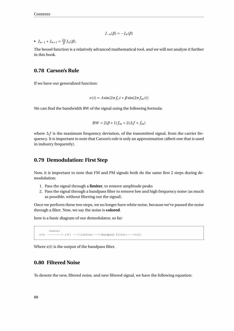
Contents

J−n(β) =−Jn(β)

• Jn−1 + Jn+1 = 2nβ Jn(β).

The bessel function is a relatively advanced mathematical tool, and we will not analyze it furtherin this book.

0.78 Carson’s Rule

If we have our generalized function:

v(t ) = A sin(2π fc t +βsin(2π fm t ))

We can find the bandwidth BW of the signal using the following formula:

BW = 2(β+1) fm = 2(∆ f + fm)

where ∆ f is the maximum frequency deviation, of the transmitted signal, from the carrier fre-quency. It is important to note that Carson’s rule is only an approximation (albeit one that is usedin industry frequently).

0.79 Demodulation: First Step

Now, it is important to note that FM and PM signals both do the same first 2 steps during de-modulation:

1. Pass the signal through a limiter, to remove amplitude peaks2. Pass the signal through a bandpass filter to remove low and high frequency noise (as much

as possible, without filtering out the signal).

Once we perform these two steps, we no longer have white noise, because we’ve passed the noisethrough a filter. Now, we say the noise is colored.

here is a basic diagram of our demodulator, so far:

channels(t) ---------> r(t) --->|Limiter|--->|Bandpass Filter|---->z(t)

Where z(t) is the output of the bandpass filter.

0.80 Filtered Noise

To denote the new, filtered noise, and new filtered signal, we have the following equation:

88

Noise Analysis

z(t ) = γA cos(Ψ(t ))+n0(t )

Where we call the additive noise n0(t ) because it has been filtered, and is not white noise any-more. n0(t ) is known as narrow band noise, and can be denoted as such:

n0(t ) = W(t )cos(2π fc t )+Z(t )sin(2π fc t )

Now, once we have it in this form, we can use a trigonometric identity to make this equationmore simple:

n0(t ) = R(t )cos(2π fc t +Θ(t ))

Where

R(t ) =√

W(t )2 +Z(t )2

Θ(t ) = t an−1(Z(t )/W(t))

Here, the new noise parameter R(t) is a rayleigh random variable, and is discussed in the nextchapter.

0.81 Noise Analysis

R(t) is a noise function that affects the amplitude of our received signal. However, our receiverpasses the signal through a limiter, which will remove amplitude fluctuations from our signal.For this reason, R(t) doesnt affect our signal, and can be safely ignored for now. This meansthat the only random variable that is affecting our signal is the variable Θ(t ), "Theta". Theta isa uniform random variable, with values between pi and -pi. Values outside this range "Wraparound" because phase is circular.

0.81.1 Section 3: Transmission

This page will discuss some of the fundamental basics of EM wave propagation.

0.82 Electromagnetic Spectrum

ELECTROMAGNETIC_WAVE34

34 HTTP://EN.WIKIPEDIA.ORG/WIKI/ELECTROMAGNETIC_WAVE

89

Contents

Figure 84

0.83 Radio Waves

RADIO_WAVES35

Maxwell first predicted the existence of electromagnetic waves in the 19th century. He came tothis conclusion by careful examination of the equations describing electric and magnetic phe-nomenon. It was left up to Hertz to create these waves, and Marconi to exploit them.

In spite of one hundred years of study, exactly what radio waves are and why they exist, remainsomewhat of a mystery.

Electromagnetic waves in free space, or TEM waves, consist of electric and magnetic fields, eachat right angles to each other and the direction of propagation.

Figure 85

35 HTTP://EN.WIKIPEDIA.ORG/WIKI/RADIO_WAVES

90

Radio Waves

The relationship between wavelength and frequency is give by:

c =λ f

where c is the speed of light (approximately 300,000,000 m/s in vacuum),f is the frequency of the wave, and is the wavelength of the wave.

Radio waves can be reflected and refracted in a manner similar to light. They are affected by theground terrain, atmosphere and other objects.

Maxwell’s equations state that a time varying magnetic field produces an electric field and a timevarying electric field produces a magnetic field. This is kind of a chicken and egg situation.

Radio waves propagate outward from an antenna, at the speed of light. The exact nature ofthese waves is determined by the transmission medium. In free space, they travel in straightlines, whereas in the atmosphere, they generally travel in a curved path. In a confined or guidedmedium, radio waves do not propagate in the TEM mode, but rather in a TE or TM mode.

Radio waves interact with objects in three principle ways:

Reflection – A radio wave bounces off an object larger than its wavelength.

Diffraction – Waves bend around objects.Scattering – A radiowave bounces off an object smaller than its wave-length.

Because of these complex interactions, radio wave propagation is often examined in three dis-tinct regions in order to simplify the analysis:

Surface (or ground) waves are located very near the earth’s surface.Space waves occur in the lower atmosphere (troposphere).Sky waves occur in the upper atmosphere (ionosphere).

The boundaries between these regions are somewhat fuzzy. In many cases, it is not possible toexamine surface waves without considering space waves.

91

Contents

Figure 86

92

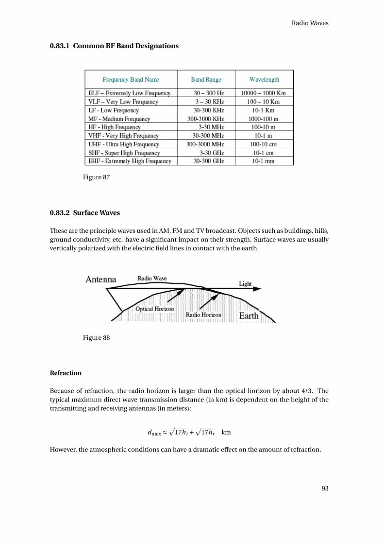
Radio Waves

0.83.1 Common RF Band Designations

Figure 87

0.83.2 Surface Waves

These are the principle waves used in AM, FM and TV broadcast. Objects such as buildings, hills,ground conductivity, etc. have a significant impact on their strength. Surface waves are usuallyvertically polarized with the electric field lines in contact with the earth.

Figure 88

Refraction

Because of refraction, the radio horizon is larger than the optical horizon by about 4/3. Thetypical maximum direct wave transmission distance (in km) is dependent on the height of thetransmitting and receiving antennas (in meters):

dmax ≈√

17ht +√

17hr km

However, the atmospheric conditions can have a dramatic effect on the amount of refraction.

93

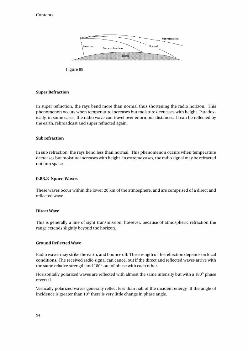
Contents

Figure 89

Super Refraction

In super refraction, the rays bend more than normal thus shortening the radio horizon. Thisphenomenon occurs when temperature increases but moisture decreases with height. Paradox-ically, in some cases, the radio wave can travel over enormous distances. It can be reflected bythe earth, rebroadcast and super refracted again.

Sub refraction

In sub refraction, the rays bend less than normal. This phenomenon occurs when temperaturedecreases but moisture increases with height. In extreme cases, the radio signal may be refractedout into space.

0.83.3 Space Waves

These waves occur within the lower 20 km of the atmosphere, and are comprised of a direct andreflected wave.

Direct Wave

This is generally a line of sight transmission, however, because of atmospheric refraction therange extends slightly beyond the horizon.

Ground Reflected Wave

Radio waves may strike the earth, and bounce off. The strength of the reflection depends on localconditions. The received radio signal can cancel out if the direct and reflected waves arrive withthe same relative strength and 180o out of phase with each other.

Horizontally polarized waves are reflected with almost the same intensity but with a 180o phasereversal.

Vertically polarized waves generally reflect less than half of the incident energy. If the angle ofincidence is greater than 10o there is very little change in phase angle.

94

Fading and Interference

0.83.4 Sky Waves

These waves head out to space but are reflected or refracted back by the ionosphere. The heightof the ionosphere ranges from 50 to 600 km.

Radio waves are refracted by the ionized gas created by solar radiation. The amount of ionizationdepends on the time of day, season and the position in the 11-year sun spot cycle. The specificradio frequency refracted is a function of electron density and launch angle.

A communication channel thousands of kilometers long can be established by successive reflec-tions at the earth’s surface and in the upper atmosphere. This ionospheric propagation takesplace mainly in the HF band.

The ionosphere is composed of several layers, which vary according to the time of day. Eachlayer has different propagation characteristics:

D layer – This layer occurs only during the day at altitudes of 60 to 90 km.High absorption takes place at frequencies up to 7 MHz.

E layer – This layer occurs at altitudes of 100 to 125 km. In the sum-mer, dense ionization clouds can form for short periods. These cloudscalled sporadic E can refract radio signals in the VHF spectrum. Thisphenomenon allows amateur radio operators to communicate over enor-mous distances.

F layer - This single nighttime layer splits into two layers (F1 and F2) dur-ing the day. The F1 layer forms at about 200 km and F2 at about 400 km.The F2 layer propagates most HF short-wave transmissions.

Because radio signals can take many paths to the receiver, multipath fading can occur. If thesignals arrive in phase, the result is a stronger signal. If they arrive out of phase with each other,they tend to cancel.

Deep fading, lasting from minutes to hours over a wide frequency range, can occur when solarflares increase the ionization in the D layer.

The useful transmission band ranges between the LUF (lowest usable frequency) and MUF (max-imum usable frequency). Frequencies above the MUF are refracted into space. Below the LUF,radio frequencies suffer severe absorption. If a signal is near either of these two extremes, it maybe subject to fading.

Meteors create ionization trails that reflect radio waves. Although these trails exist for only a fewseconds, they have been successfully used in communications systems spanning 1500 km.

The Aurora Borealis or Northern Lights cause random reflection in the 3 - 5 MHz region. Auroracauses signal flutter at 100 Hz to 2000 Hz thus making voice transmission impossible.

0.84 Fading and Interference

Radio signals may vary in intensity for many reasons.

95

Contents

0.84.1 Flat Earth Reflections (Horizontal Polarization)

There are at least two possible paths for radio waves to travel when the antennas are near theearth: direct path and reflected path. These two signals interact in a very complex manner. How-ever, ignoring polarization and assuming a flat earth can produce some interesting mathematicaldescriptions.

Figure 90

p1 = direct wave path length

p2 = reflected wave path length

∆

p = p2 - p1 difference in path lengths

d = distance

From the geometry we can observe:

p21 = (hr −ht )2 +d 2

p22 = (hr +ht )2 +d 2

p22 −p2

1 = (hr −ht )2 +d 2 − (hr +ht )2 −d 2 = 4hr ht

(p2 −p1

)(p2 +p1

)= 4hr ht

But∆p = (p2 −p1

)and d ≈ p1 ≈ p2

96

Fading and Interference

∆p2d ≈ 4hr ht

therefore

∆p ≈ 2hr ht

d

If the difference in the two paths ∆p, is 1/2 λ long, the two signals tend to cancel. If ∆p is equalto λ, the two signals tend to reinforce. The path difference ∆p therefore corresponds to a phaseangle change of:

ϕp = 2π

λ∆p = 4πhr ht

λd

The resultant received signal is the sum of the two components. The situation is unfortunatelymade more complex by the fact that the phase integrity of the reflected wave is not maintainedat the point of reflection.

If we limit the examination of reflected waves to the horizontally polarized situation, we obtainthe following geometry:

Figure 91

Applying the cosine rule to this diagram, we obtain a resultant signal of:

Er = E1

√2(1−cosϕp

)= 2E1 sin(ϕp

2

)The signal strength of the direct wave is the unit distance value divided by the distance: Er = E0

dTherefore, the received signal can be written as:

Er = 2E0

dsin

(2πhr ht

λd

)For small angles this can be approximated by:

Er ≈ 2E0

d

2πhr ht

λd= E0

4πhr ht

λd 2

97

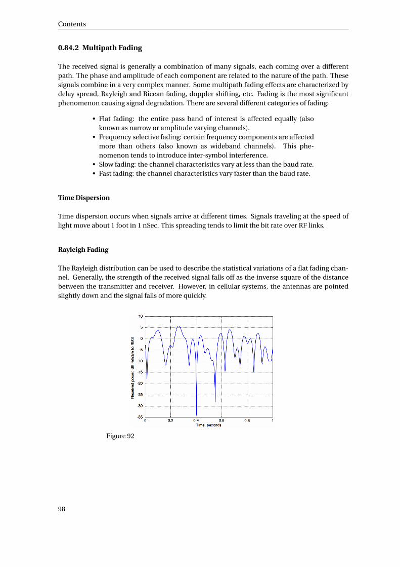
Contents

0.84.2 Multipath Fading

The received signal is generally a combination of many signals, each coming over a differentpath. The phase and amplitude of each component are related to the nature of the path. Thesesignals combine in a very complex manner. Some multipath fading effects are characterized bydelay spread, Rayleigh and Ricean fading, doppler shifting, etc. Fading is the most significantphenomenon causing signal degradation. There are several different categories of fading:

• Flat fading: the entire pass band of interest is affected equally (alsoknown as narrow or amplitude varying channels).

• Frequency selective fading: certain frequency components are affectedmore than others (also known as wideband channels). This phe-nomenon tends to introduce inter-symbol interference.

• Slow fading: the channel characteristics vary at less than the baud rate.• Fast fading: the channel characteristics vary faster than the baud rate.

Time Dispersion

Time dispersion occurs when signals arrive at different times. Signals traveling at the speed oflight move about 1 foot in 1 nSec. This spreading tends to limit the bit rate over RF links.

Rayleigh Fading

The Rayleigh distribution can be used to describe the statistical variations of a flat fading chan-nel. Generally, the strength of the received signal falls off as the inverse square of the distancebetween the transmitter and receiver. However, in cellular systems, the antennas are pointedslightly down and the signal falls of more quickly.

Figure 92

98

Fading and Interference

Ricean Fading

The Ricean distribution is used to describe the statistical variations of signals with a strong di-rect or line-of-sight component and numerous weaker reflected ones. This can happen in anymultipath environment such as inside buildings or in an urban center.

A received signal is generally comprised of several signals, each taking a slightly different path.Since some may add constructively in-phase and others out of phase, the overall signal strengthmay vary by 40 dB or more if the receiver is moved even a very short distance.

Doppler Shift

A frequency shift is caused by the relative motion of the transmitter and receiver, or any objectthat reflects/refracts signal. This movement creates random frequency modulation. Dopplerfrequency shift is either positive or negative depending on whether the transmitter is movingtowards or away from the receiver.

This Doppler frequency shift is given by:

fd = vm

cfc

vm is the relative motion of the transmitter with respect to the receiver, c is the speed of light andfc is the transmitted frequency. In the multipath environment, the relative movement of eachpath is generally different. Thus, the signal is spread over a band of frequencies. This is knownas the Doppler spread.

0.84.3 Atmospheric Diffraction

Radio waves cannot penetrate very far into most objects. Consequently, there is often a shadowzone behind objects such as buildings, hills, etc.

The radio shadow zone does not have a very sharp cutoff due to spherical spreading, also calledHuygens’ principle. Each point on a wavefront acts as it were a point source radiating along thepropagation path. The overall wavefront is the vector sum of all the point sources or wavelets.The wavelet magnitude is proportional to 1+ cosθ where θ is measured from the direction ofpropagation. The amplitude is a maximum in the direction of propagation and zero in the re-verse direction.

99

Contents

0.85 Reflection

0.86 Diffraction

0.87 Path Loss

0.88 Rayleigh Fading

0.89 Rician Fading

0.90 Doppler Shift

This page is going to talk about the effect of noise on transmission systems.

0.91 Types of Noise

ELECTRONIC_NOISE36

Most man made electro-magnetic noise occurs at frequencies below 500 MHz. The most signif-icant of these include:

• Hydro lines• Ignition systems• Fluorescent lights• Electric motors

Therefore deep space networks are placed out in the desert, far from these sources of interfer-ence.

There are also a wide range of natural noise sources which cannot be so easily avoided, namely:

•Atmospheric noise - lighting < 20 MHz•Solar noise - sun - 11 year sunspot cycle•Cosmic noise - 8 MHz to 1.5 GHz•Thermal or Johnson noise. Due to free electrons striking vibrating ions.•White noise - white noise has a constant spectral density over a specifiedrange of frequencies. Johnson noise is an example of white noise.•Gaussian noise - Gaussian noise is completely random in nature how-ever, the probability of any particular amplitude value follows the normaldistribution curve. Johnson noise is Gaussian in nature.•Shot noise - bipolar transistors

36 HTTP://EN.WIKIPEDIA.ORG/WIKI/ELECTRONIC_NOISE

100

Types of Noise

in =√

2q Idc∆ f

where q = electron charge 1.6 x 10-17 coulombs

•Excess noise, flicker, 1/f, and pink noise < 1 KHz are Inversely proportionalto frequency and directly proportional to temperature and dc current•Transit time noise - occurs when the electron transit time across a junc-tion is the same period as the signal.

Of these, only Johnson noise can be readily analysed and compensated for. The noise power isgiven by:

Pn = kT B

Where:

k = Boltzman’s constant (1.38 x 10-23 J/K)T = temperature in degrees KelvinB = bandwidth in Hz

This equation applies to copper wire wound resistors, but is close enough to be used for all re-sistors. Maximum power transfer occurs when the source and load impedance are equal.

0.91.1 Combining Noise Voltages

The instantaneous value of two noise voltages is simply the sum of their individual values at thesame instant.

vtot al i nst = v1 i nst + v2 i nst

This result is readily observable on an oscilloscope. However, it is not particularly helpful, sinceit does not result in a single stable numerical value such as one measured by a voltmeter.

If the two voltages are coherent [K = 1], then the total rms voltage value is the sum of the individ-ual rms voltage values.

vtot al r ms = v1 r ms + v2 r ms

If the two signals are completely random with respect to each other [K = 0], such as Johnson noisesources, the total power is the sum of all of the individual powers:

Ptot al r andom noi se = Pn1 r andom +Pn2 r andom

101

Contents

A Johnson noise of power P = kTB, can be thought of as a noise voltage applied through a resistor,Thevenin equivalent.

Figure 93

An example of such a noise source may be a cable or transmission line. The amount of noisepower transferred from the source to a load, such as an amplifier input, is a function of the sourceand load impedances.

102

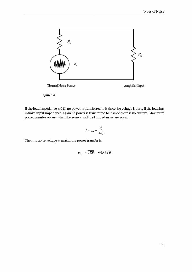
Types of Noise

Figure 94

If the load impedance is 0Ω, no power is transferred to it since the voltage is zero. If the load hasinfinite input impedance, again no power is transferred to it since there is no current. Maximumpower transfer occurs when the source and load impedances are equal.

PL max =e2

s

4Rs

The rms noise voltage at maximum power transfer is:

en =p

4RP =p

4RkT B

103

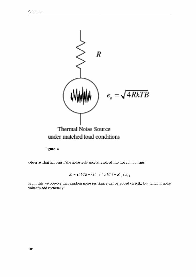
Contents

Figure 95

Observe what happens if the noise resistance is resolved into two components:

e2n = 4RkT B = 4(R1 +R2)kT B = e2

n1 +e2n2

From this we observe that random noise resistance can be added directly, but random noisevoltages add vectorially:

104

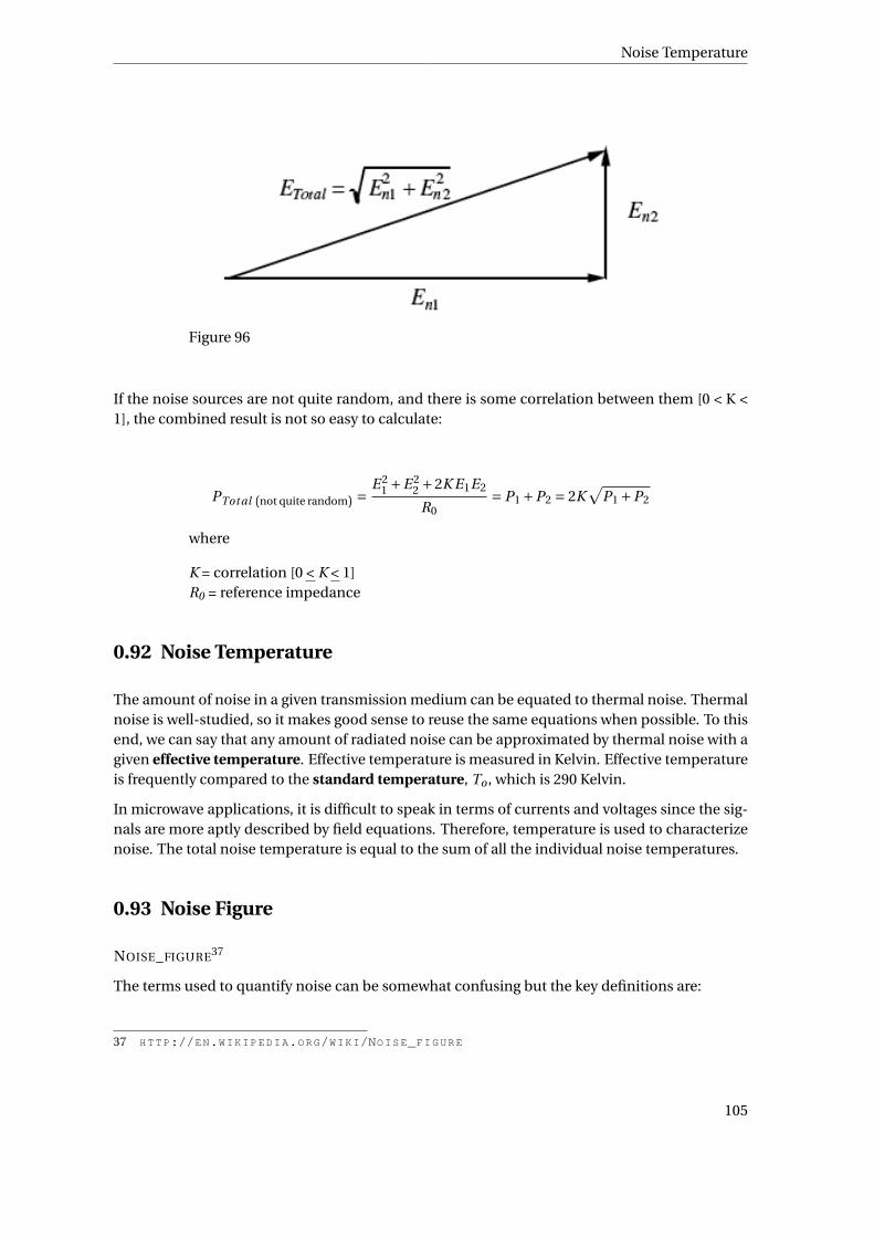
Noise Temperature

Figure 96

If the noise sources are not quite random, and there is some correlation between them [0 < K <1], the combined result is not so easy to calculate:

PTot al (not quite random) =E 2

1 +E 22 +2K E1E2

R0= P1 +P2 = 2K

√P1 +P2

where

K = correlation [0 < K < 1]R0 = reference impedance

0.92 Noise Temperature

The amount of noise in a given transmission medium can be equated to thermal noise. Thermalnoise is well-studied, so it makes good sense to reuse the same equations when possible. To thisend, we can say that any amount of radiated noise can be approximated by thermal noise with agiven effective temperature. Effective temperature is measured in Kelvin. Effective temperatureis frequently compared to the standard temperature, To , which is 290 Kelvin.

In microwave applications, it is difficult to speak in terms of currents and voltages since the sig-nals are more aptly described by field equations. Therefore, temperature is used to characterizenoise. The total noise temperature is equal to the sum of all the individual noise temperatures.

0.93 Noise Figure

NOISE_FIGURE37

The terms used to quantify noise can be somewhat confusing but the key definitions are:

37 HTTP://EN.WIKIPEDIA.ORG/WIKI/NOISE_FIGURE

105

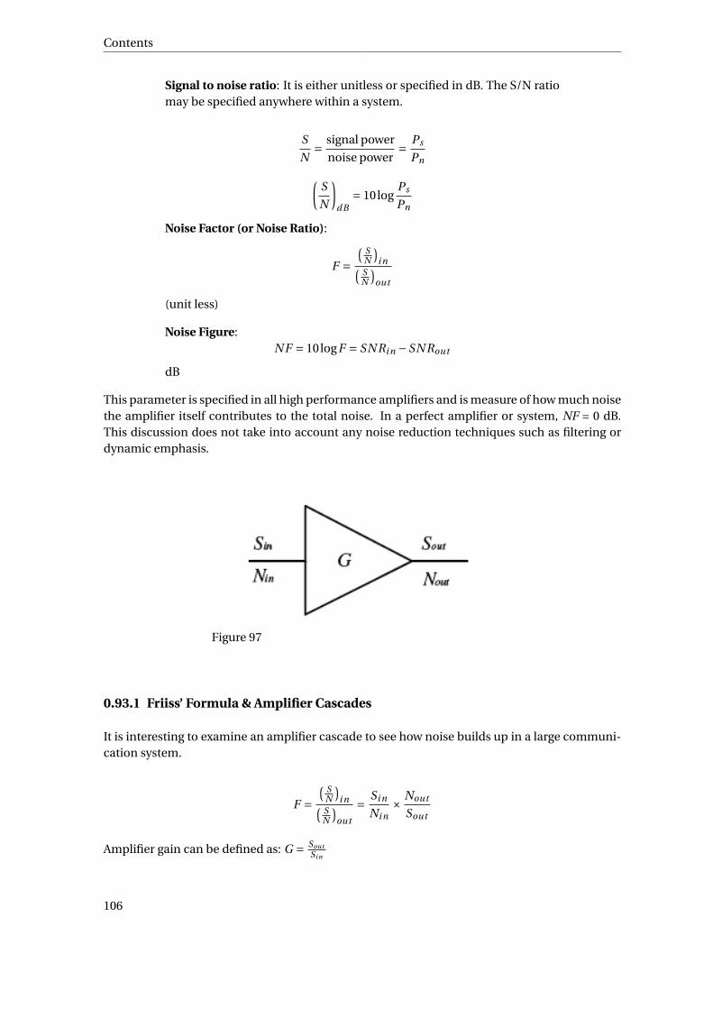
Contents

Signal to noise ratio: It is either unitless or specified in dB. The S/N ratiomay be specified anywhere within a system.

S

N= signal power

noise power= Ps

Pn(S

N

)dB

= 10logPs

Pn

Noise Factor (or Noise Ratio):

F =( S

N

)i n( S

N

)out

(unit less)

Noise Figure:N F = 10logF = SN Ri n −SN Rout

dB

This parameter is specified in all high performance amplifiers and is measure of how much noisethe amplifier itself contributes to the total noise. In a perfect amplifier or system, NF = 0 dB.This discussion does not take into account any noise reduction techniques such as filtering ordynamic emphasis.

Figure 97

0.93.1 Friiss’ Formula & Amplifier Cascades

It is interesting to examine an amplifier cascade to see how noise builds up in a large communi-cation system.

F =( S

N

)i n( S

N

)out

= Si n

Ni n× Nout

Sout

Amplifier gain can be defined as: G = SoutSi n

106

Noise Figure

Figure 98

Therefore the output signal power is:

Sout =GSi n

and the noise factor (ratio) can be rewritten as:

F = Si n

Ni n× Nout

GSi n= Nout

GNi n

The output noise power can now be written:

Nout = FGNi n

From this we observe that the input noise is increased by the noise ratio and amplifier gain as itpasses through the amplifier. A noiseless amplifier would have a noise ratio (factor) of 1 or noisefigure of 0 dB. In this case, the input noise would only be amplified by the gain since the amplifierwould not contribute noise.

The minimum noise that can enter any system is the Johnson Noise:

Ni n(minimum) = kT B

Therefore the minimum noise that can appear at the output of any am-plifier is:

Nout (minimum) = FGkT B

The output noise of a perfect amplifier would be (F = 1):

Nout(perfect) =GkT B

The difference between these two values is the noised created (added) bythe amplifier itself:

107

Contents

Nout (added) = Nout (minimum)−Nout(perfect) = FGkT B−GkT B = (F −1)GkT B

This is the additional (created) noise, appearing at the output.

The total noise out of the amplifier is then given by:

Ntot al = Nout(perfect)+Nout (added) =GkT B+(F −1)GkT B

If a second amplifier were added in series, the total output noise would consist the first stagenoise amplified by the second stage gain, plus the additional noise of the second amplifier:

Ntot al =G1G2kT B + (F1 −1)G1G2kT B + (F2 −1)G2kT B

If we divide both sides of this expression by the common term:

G1G2kT B

we obtain:

Ntot al

G1G2kT B= G1G2kT B + (F1 −1)G1G2kT B + (F2 −1)G2kT B

G1G2kT B

Recall:

F = Nout

GNi n= Ntot al

G1G2kT B

Then:

Fover al l = F1 + F2 −1

G1

This process can be extended to include more amplifiers in cascade to arrive at:

Friiss’ Formula

F = F1 + F2 −1

G1+ F3 −1

G1G2+

This equation shows that the overall system noise figure is largely determined by the noise figureof the first stage in a cascade since the noise contribution of any stage is divided by the gains ofthe preceding stages. This is why the 1st stage in any communication system should be an LNA(low noise amplifier).

108

Receiver Sensitivity

0.94 Receiver Sensitivity

In a given bandwidth, W, we can show that the noise power N equals:

N = F (kT0)W

From N, we can show that the sensitivity of the receiver is equal to

SN R ×N

0.95 Cascaded Systems

This page will discuss the topic of signal propagation through physical mediums, such as wires.

0.96 Transmission Line Equation

TRANSMISSION_LINE38

Many kinds of communication systems require signals at some point to be conveyed over copperwires.

The following analysis requires two assumptions:

• A transmission line can be decomposed into small, distributed passiveelectrical elements• These elements are independent of frequency (i.e. although reactance isa function of frequency, resistance, capacitance and inductance are not)

These two assumptions limit the following analysis to frequencies up to the low MHz region.The second assumption is particularly difficult to defend since it is well known that the resis-tance of a wire increases with frequency because the conduction cross-section decreases. Thisphenomenon is known as the skin effect and is not easy to evaluate.

38 HTTP://EN.WIKIPEDIA.ORG/WIKI/TRANSMISSION_LINE

109

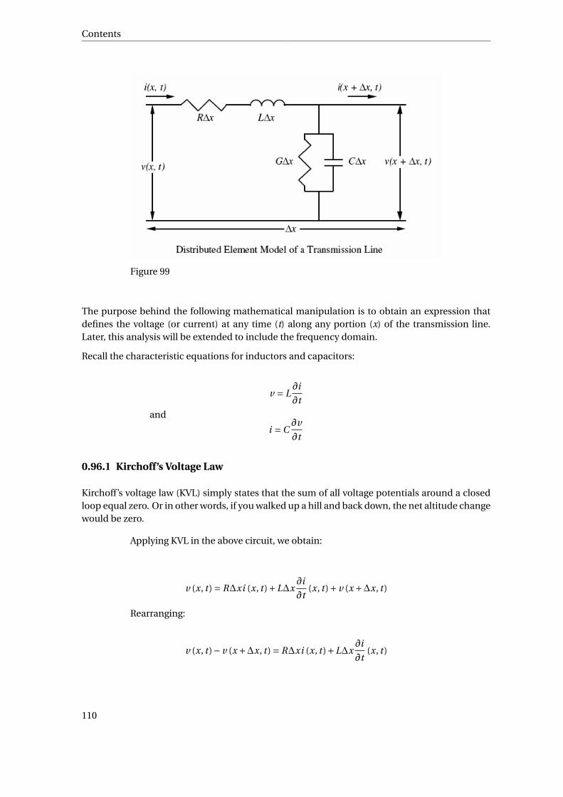
Contents

Figure 99

The purpose behind the following mathematical manipulation is to obtain an expression thatdefines the voltage (or current) at any time (t) along any portion (x) of the transmission line.Later, this analysis will be extended to include the frequency domain.

Recall the characteristic equations for inductors and capacitors:

v = L∂i

∂t

and

i =C∂v

∂t

0.96.1 Kirchoff’s Voltage Law

Kirchoff’s voltage law (KVL) simply states that the sum of all voltage potentials around a closedloop equal zero. Or in other words, if you walked up a hill and back down, the net altitude changewould be zero.

Applying KVL in the above circuit, we obtain:

v (x, t ) = R∆xi (x, t )+L∆x∂i

∂t(x, t )+ v (x +∆x, t )

Rearranging:

v (x, t )− v (x +∆x, t ) = R∆xi (x, t )+L∆x∂i

∂t(x, t )

110

Transmission Line Equation

But the LHS (left hand side) of the above equation, represents the voltagedrop across the cable element

∆v

, therefor:

∆v = R∆xi (x, t )+L∆x∂i

∂t(x, t )

Dividing through by∆x

, we obtain:

∆v

∆x= Ri (x, t )+L

∂i

∂t(x, t )

The LHS is easily recognized as a derivative. Simplifying the notation:

∂v

∂x= Ri +L

∂i

∂t

This expression has both current and voltage in it. It would be convenient to write the equationin terms of current or voltage as a function of distance or time.

0.96.2 Simplifying the Equation (trust me)

The first step in separating voltage and current is to take the derivative with respect to the posi-tion x (Equation 1):

∂2v

∂x2 = R∂i

∂x+L

∂2i

∂x∂t

The next step is to eliminate the current terms, leaving an expression withvoltage only. The change in current along the line is equal to the cur-rent being shunted across the line through the capacitance C and con-ductance G. By applying KCL in the circuit, we obtain the necessary infor-mation (Equation 2):

∂i

∂x=Gv +C

∂v

∂t

Taking the derivative with respect to time, we obtain (Equation 3):

∂2i

∂x∂t=G

∂v

∂t+C

∂2v

∂t 2

Substituting (Equation 2) and (Equation 3) into (Equation 1), we obtainthe desired simplification:

111

Contents

∂2v

∂x2 = R

[Gv +C

∂v

∂t

]+L

[G∂v

∂t+C

∂2v

∂t 2

]Collecting the terms, we obtain:

The Transmission Line Equation for Voltage

∂2v

∂x2 = RGv + (RC +LG)∂v

∂t+LC

∂2v

∂t 2

This equation is known as the transmission line equation. Note that it has voltage at any partic-ular location x as a function of time t.

Similarly for current, we obtain:

The Transmission Line Equation for Current

∂2i

∂x2 = RGi + (RC +LG)∂i

∂t+LC

∂2i

∂t 2

But we’re not quite done yet.

0.96.3 Solving the Transmission Line Equation

Historically, a mathematician would solve the transmission line equation for v by assuming a so-lution for v, substituting it into the equation, and observing whether the result made any sense.An engineer would follow a similar procedure by making an “educated guess” based on somelaboratory experiments, as to what the solution might be. Today there are more sophisticatedtechniques used to find solutions. In this respect, the engineer may lag behind the mathemati-cian by several centuries in finding applications for mathematical tools.

To solve the transmission line equation, we shall guess that the solution for the voltage functionis of the form:

v (t ) = e jωt e−γx

The first term represents a unity vector rotating at an angular velocity of ω radians per second,in other words, a sine wave of some frequency. The second term denotes the sinusoid beingmodified by the transmission line, namely its amplitude decaying exponentially with distance. Ifwe let γ be a complex quantity, we can also include any phase changes which occur as the signaltravels down the line.

The sine wave is used as a signal source because it is easy to generate, and manip-ulate mathematically. Euler’s Identity shows the relationship between exponentialnotation and trigonometric functions:

Euler’s Identity

112

Transmission Line Equation

e jωt = cos(ωt )+ j sin(ωt )

Going back to our educated guess, we will let

γ=α+ jβ

, therefore:

v (t ) = e jωt e−(α+ jβ)x = e−αx e(ωt−βx) j

The terme−αx

represents the exponential amplitude decay as this signal travels downthe line.

α

is known as the attenuation coefficient and is expressed in Nepers permeter.

The terme(ωt−βx) j

represents the frequency of the signal at any point along the line.

β

component is known as the phase shift coefficient, and is expressed inradians per meter.

Substituting our educated guess

v (t ) = e jωt e−(α+ jβ)x

into the transmission line equation for voltage, we obtain:

∂2

∂x2

[e jωt e−(α+ jβ)x

]= RG

[e jωt e−(α+ jβ)x

]+(RC +LG)

∂

∂t

[e jωt e−(α+ jβ)x

]+LC

∂2

∂t 2

[e jωt e−(α+ jβ)x

]This looks pretty intimidating, but if you can do basic differentials and algebra, you can do this!

Simplifying the Equation (trust me)

The idea now is to work through the math to see if we come up with a reasonable solution. If wearrive at a contradiction or an unreasonable result, it means that our educated guess was wrongand we have to do more experimenting and come up with a better guess as to how voltage andcurrent travel down a transmission line.

Let’s look at this equation one term at a time:

113

Contents

LHS = RHS Term 1 + RHS Term 2 + RHS Term 3

Starting with the left hand side (LHS) we get the following simplification:

∂2

∂x2

[e jωt e−(α+ jβ)x

]= ∂

∂x

[−(α+ jβ

)e jωt e−(α+ jβ)x

]= (

α+ jβ)2 e jωt e−(α+ jβ)x

Believe it or not, the RHS Term 1 does not need simplifying.

Simplifying the RHS Term 2, we obtain:

(RC +LG)∂

∂t

[e jωt e−(α+ jβ)x

]= (RC +LG) jω

(e jωt e−(α+ jβ)x

)Simplifying the RHS Term 3, we obtain:

LC∂2

∂t 2

[e jωt e−(α+ jβ)x

]= LC

∂

∂t

[jωe jωt e−(α+ jβ)x

]=−LCω2e jωt e−(α+ jβ)x

Let’s put it all back together:

(α+ jβ

)2 e jωt e−(α+ jβ)x = RG(e jωt e−(α+ jβ)x

)+(RC +LG) jω

(e jωt e−(α+ jβ)x

)−LCω2

(e jωt e−(α+ jβ)x

)Note that each of the four terms contain the expression

e jωt e−(α+ jβ)x

.

Therefore we end up with:

(α+ jβ

)2 = RG + (RC +LG) jω−LCω2

And this can be further simplified to:

Attenuation and Phase Shift Coefficients

α+ jβ= γ=√(

R + jωL)(

G + jωC)

This result is not self contradictory or unreasonable. Therefore we conclude that our educatedguess was right and we have successfully found an expression for attenuation and phase shift ona transmission line as a function of its distributed electrical components and frequency.

114

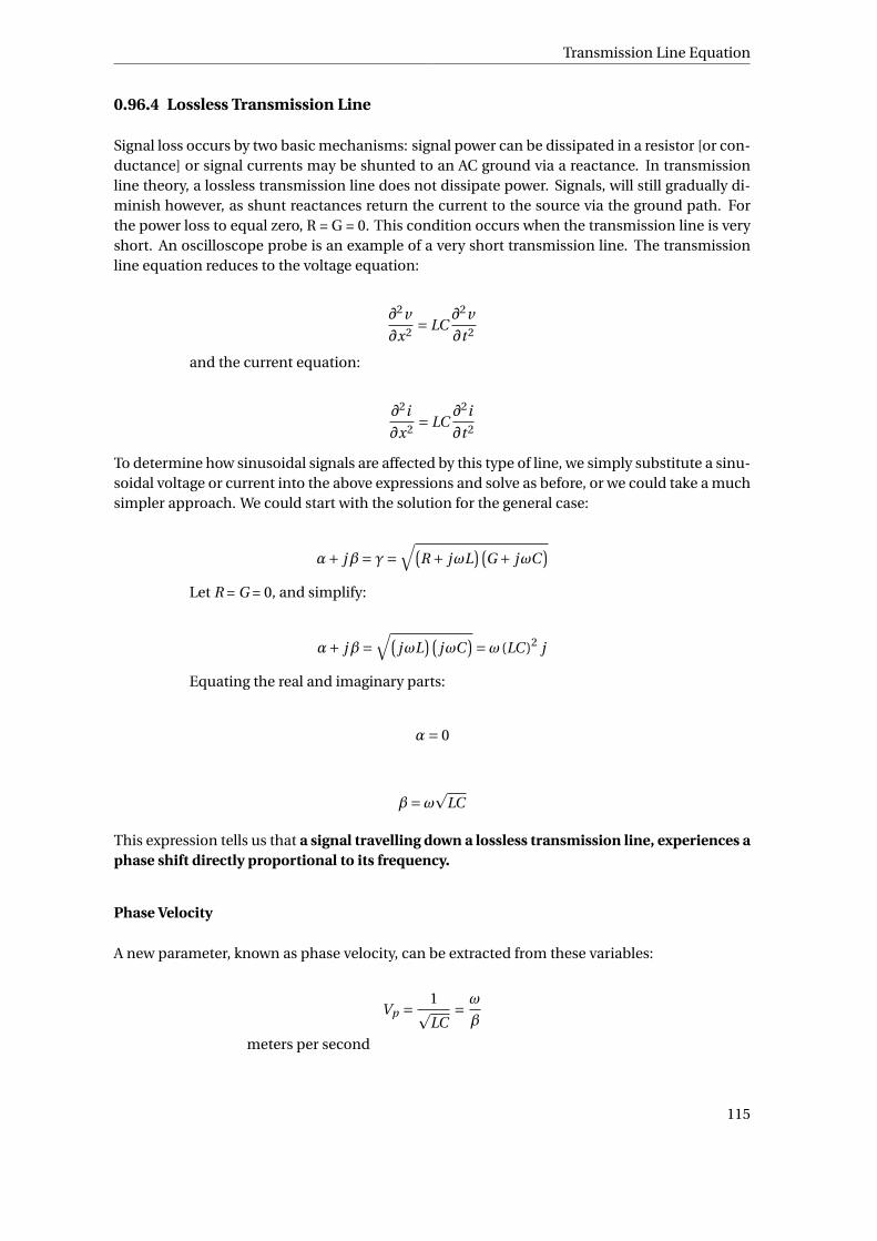
Transmission Line Equation

0.96.4 Lossless Transmission Line

Signal loss occurs by two basic mechanisms: signal power can be dissipated in a resistor [or con-ductance] or signal currents may be shunted to an AC ground via a reactance. In transmissionline theory, a lossless transmission line does not dissipate power. Signals, will still gradually di-minish however, as shunt reactances return the current to the source via the ground path. Forthe power loss to equal zero, R = G = 0. This condition occurs when the transmission line is veryshort. An oscilloscope probe is an example of a very short transmission line. The transmissionline equation reduces to the voltage equation:

∂2v

∂x2 = LC∂2v

∂t 2

and the current equation:

∂2i

∂x2 = LC∂2i

∂t 2

To determine how sinusoidal signals are affected by this type of line, we simply substitute a sinu-soidal voltage or current into the above expressions and solve as before, or we could take a muchsimpler approach. We could start with the solution for the general case:

α+ jβ= γ=√(

R + jωL)(

G + jωC)

Let R = G = 0, and simplify:

α+ jβ=√(

jωL)(

jωC)=ω (LC )2 j

Equating the real and imaginary parts:

α= 0

β=ωp

LC

This expression tells us that a signal travelling down a lossless transmission line, experiences aphase shift directly proportional to its frequency.

Phase Velocity

A new parameter, known as phase velocity, can be extracted from these variables:

Vp = 1pLC

= ω

β

meters per second

115

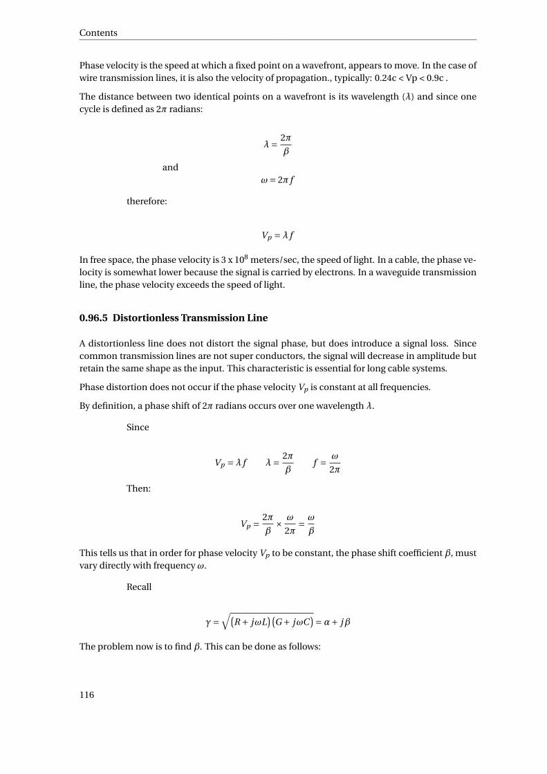
Contents

Phase velocity is the speed at which a fixed point on a wavefront, appears to move. In the case ofwire transmission lines, it is also the velocity of propagation., typically: 0.24c < Vp < 0.9c .

The distance between two identical points on a wavefront is its wavelength (λ) and since onecycle is defined as 2π radians:

λ= 2π

β

andω= 2π f

therefore:

Vp =λ f

In free space, the phase velocity is 3 x 108 meters/sec, the speed of light. In a cable, the phase ve-locity is somewhat lower because the signal is carried by electrons. In a waveguide transmissionline, the phase velocity exceeds the speed of light.

0.96.5 Distortionless Transmission Line

A distortionless line does not distort the signal phase, but does introduce a signal loss. Sincecommon transmission lines are not super conductors, the signal will decrease in amplitude butretain the same shape as the input. This characteristic is essential for long cable systems.

Phase distortion does not occur if the phase velocity Vp is constant at all frequencies.

By definition, a phase shift of 2π radians occurs over one wavelength λ.

Since

Vp =λ f λ= 2π

βf = ω

2π

Then:

Vp = 2π

β× ω

2π= ω

β

This tells us that in order for phase velocity Vp to be constant, the phase shift coefficient β, mustvary directly with frequency ω.

Recall

γ=√(

R + jωL)(

G + jωC)=α+ jβ

The problem now is to find β. This can be done as follows:

116

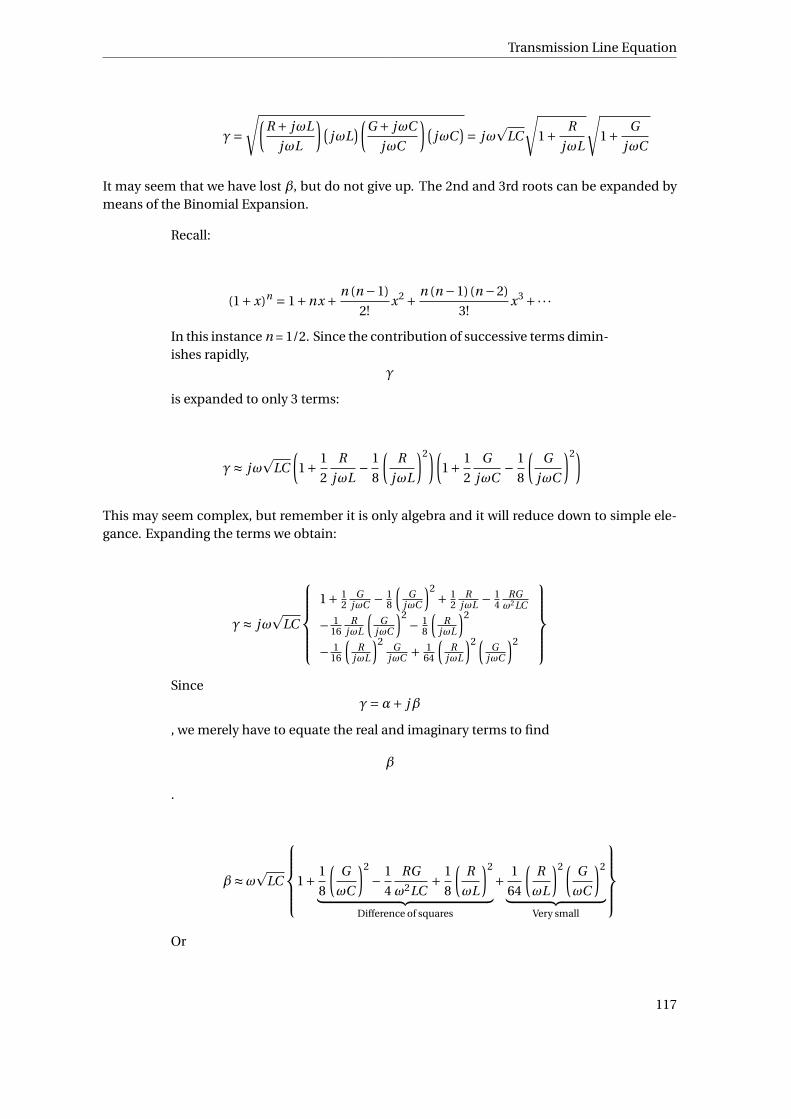
Transmission Line Equation

γ=√(

R + jωL

jωL

)(jωL

)(G + jωC

jωC

)(jωC

)= jωp

LC

√1+ R

jωL

√1+ G

jωC

It may seem that we have lost β, but do not give up. The 2nd and 3rd roots can be expanded bymeans of the Binomial Expansion.

Recall:

(1+x)n = 1+nx + n (n −1)

2!x2 + n (n −1)(n −2)

3!x3 +·· ·

In this instance n = 1/2. Since the contribution of successive terms dimin-ishes rapidly,

γ

is expanded to only 3 terms:

γ≈ jωp

LC

(1+ 1

2

R

jωL− 1

8

(R

jωL

)2)(1+ 1

2

G

jωC− 1

8

(G

jωC

)2)

This may seem complex, but remember it is only algebra and it will reduce down to simple ele-gance. Expanding the terms we obtain:

γ≈ jωp

LC

1+ 1

2G

jωC − 18

(G

jωC

)2 + 12

RjωL − 1

4RGω2LC

− 116

RjωL

(G

jωC

)2 − 18

(R

jωL

)2

− 116

(R

jωL

)2G

jωC + 164

(R

jωL

)2 (G

jωC

)2

Since

γ=α+ jβ

, we merely have to equate the real and imaginary terms to find

β

.

β≈ωp

LC

1+ 1

8

(G

ωC

)2

− 1

4

RG

ω2LC+ 1

8

(R

ωL

)2

︸ ︷︷ ︸Difference of squares

+ 1

64

(R

ωL

)2 (G

ωC

)2

︸ ︷︷ ︸Very small

Or

117

Contents

β≈ωp

LC

1+ 1

8

(R

ωL− G

ωC

)2Note that if

R

ωL= G

ωC

thenβ≈ω

pLC

From this we observe that β is directly proportional to ω.

Therefore the requirement for distortionless transmission is:

RC = LG

HEAVISIDE_CONDITION39

This is one of the essential design characteristics for a broadband coaxcable network.

If we equate the real terms, we obtain:

α≈p

RG

So there is a reason to study algebra after all!

0.97 The Frequency Domain

Signal analysis is often performed in the frequency domain. This tells us how the transmissionline affects the spectral content of the signals they are carrying.

To determine this, it is necessary to find the Fourier Transform of the transmission line equation.Recall:

∂2v

∂x2 = RGv + (RC +LG)∂v

∂t+LC

∂2v

∂t 2

and recall (hopefully) the Fourier Transform (which converts the time domain to the frequencydomain):

F

f (t )= F (ω) =

∞∫−∞

e− jωt f (t )d t

39 HTTP://EN.WIKIPEDIA.ORG/WIKI/HEAVISIDE_CONDITION

118

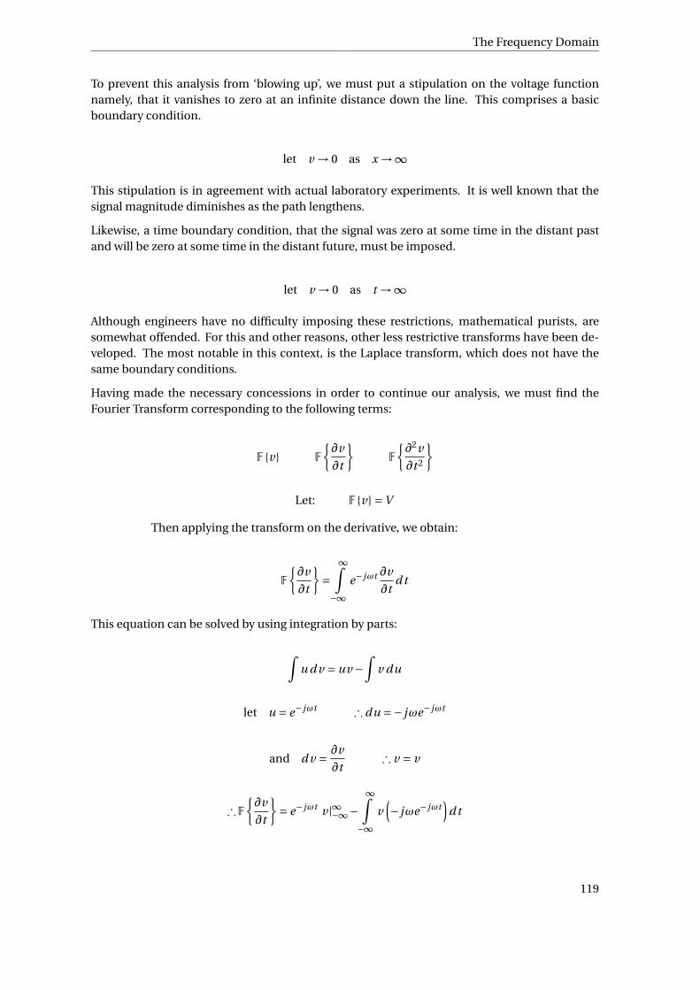
The Frequency Domain

To prevent this analysis from ‘blowing up’, we must put a stipulation on the voltage functionnamely, that it vanishes to zero at an infinite distance down the line. This comprises a basicboundary condition.

let v → 0 as x →∞

This stipulation is in agreement with actual laboratory experiments. It is well known that thesignal magnitude diminishes as the path lengthens.

Likewise, a time boundary condition, that the signal was zero at some time in the distant pastand will be zero at some time in the distant future, must be imposed.

let v → 0 as t →∞

Although engineers have no difficulty imposing these restrictions, mathematical purists, aresomewhat offended. For this and other reasons, other less restrictive transforms have been de-veloped. The most notable in this context, is the Laplace transform, which does not have thesame boundary conditions.

Having made the necessary concessions in order to continue our analysis, we must find theFourier Transform corresponding to the following terms:

F v F

∂v

∂t

F

∂2v

∂t 2

Let: F v =V

Then applying the transform on the derivative, we obtain:

F

∂v

∂t

=

∞∫−∞

e− jωt ∂v

∂td t

This equation can be solved by using integration by parts:

∫u d v = uv −

∫v du

let u = e− jωt ∴ du =− jωe− jωt

and d v = ∂v

∂t∴ v = v

∴ F

∂v

∂t

= e− jωt v |∞−∞−

∞∫−∞

v(− jωe− jωt

)d t

119

Contents

Applying the boundary conditions when t goes to infinity makes the 1st term disappear.

∴ F

∂v

∂t

= jω

∞∫−∞

e− jωt v d t

Note that the resulting integral is simply the Fourier Transform. In other words:

F

∂v

∂t

= jωF v = jωV

similarly:

F

∂2v

∂t 2

= (

jω)2F v = (

jω)2 V

We can now write the transmission line equation in the frequency domain:

∂2V

∂x2 = RGV + (RC +LG) jωV +LC(

jω)2 V

where:

V =V (ω) = F v (t )

Rearranging the terms, we obtain:

∂2V

∂x2 = [RG + (RC +LG) jω+ (

jωL)(

jωC)]

V

or

∂2V

∂x2 = [(R + jωL

)(G + jωC

)]V

since:

√(R + jωL

)(G + jωC

)=α+ jβ= γ

then

∂2V

∂x2 = γ2V

or

120

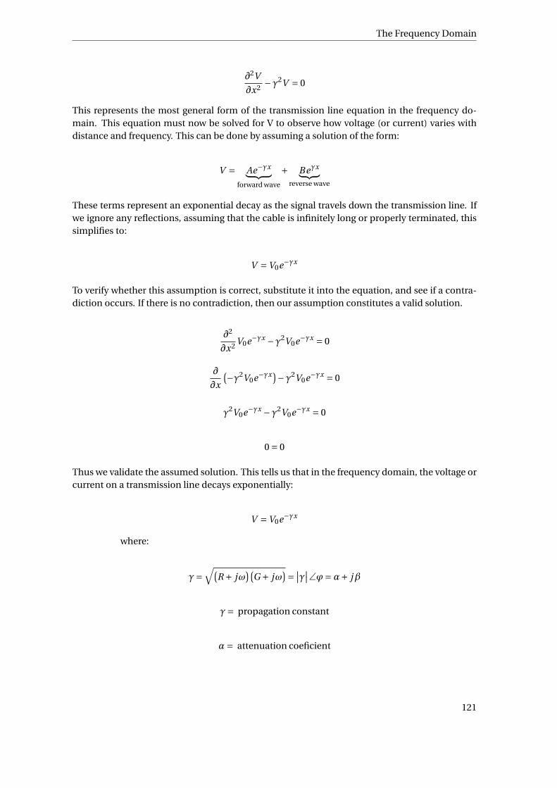
The Frequency Domain

∂2V

∂x2 −γ2V = 0

This represents the most general form of the transmission line equation in the frequency do-main. This equation must now be solved for V to observe how voltage (or current) varies withdistance and frequency. This can be done by assuming a solution of the form:

V = Ae−γx︸ ︷︷ ︸forward wave

+ Beγx︸ ︷︷ ︸reverse wave

These terms represent an exponential decay as the signal travels down the transmission line. Ifwe ignore any reflections, assuming that the cable is infinitely long or properly terminated, thissimplifies to:

V =V0e−γx

To verify whether this assumption is correct, substitute it into the equation, and see if a contra-diction occurs. If there is no contradiction, then our assumption constitutes a valid solution.

∂2

∂x2 V0e−γx −γ2V0e−γx = 0

∂

∂x

(−γ2V0e−γx)−γ2V0e−γx = 0

γ2V0e−γx −γ2V0e−γx = 0

0 = 0

Thus we validate the assumed solution. This tells us that in the frequency domain, the voltage orcurrent on a transmission line decays exponentially:

V =V0e−γx

where:

γ=√(

R + jω)(

G + jω)= ∣∣γ∣∣∠ϕ=α+ jβ

γ= propagation constant

α= attenuation coeficient

121

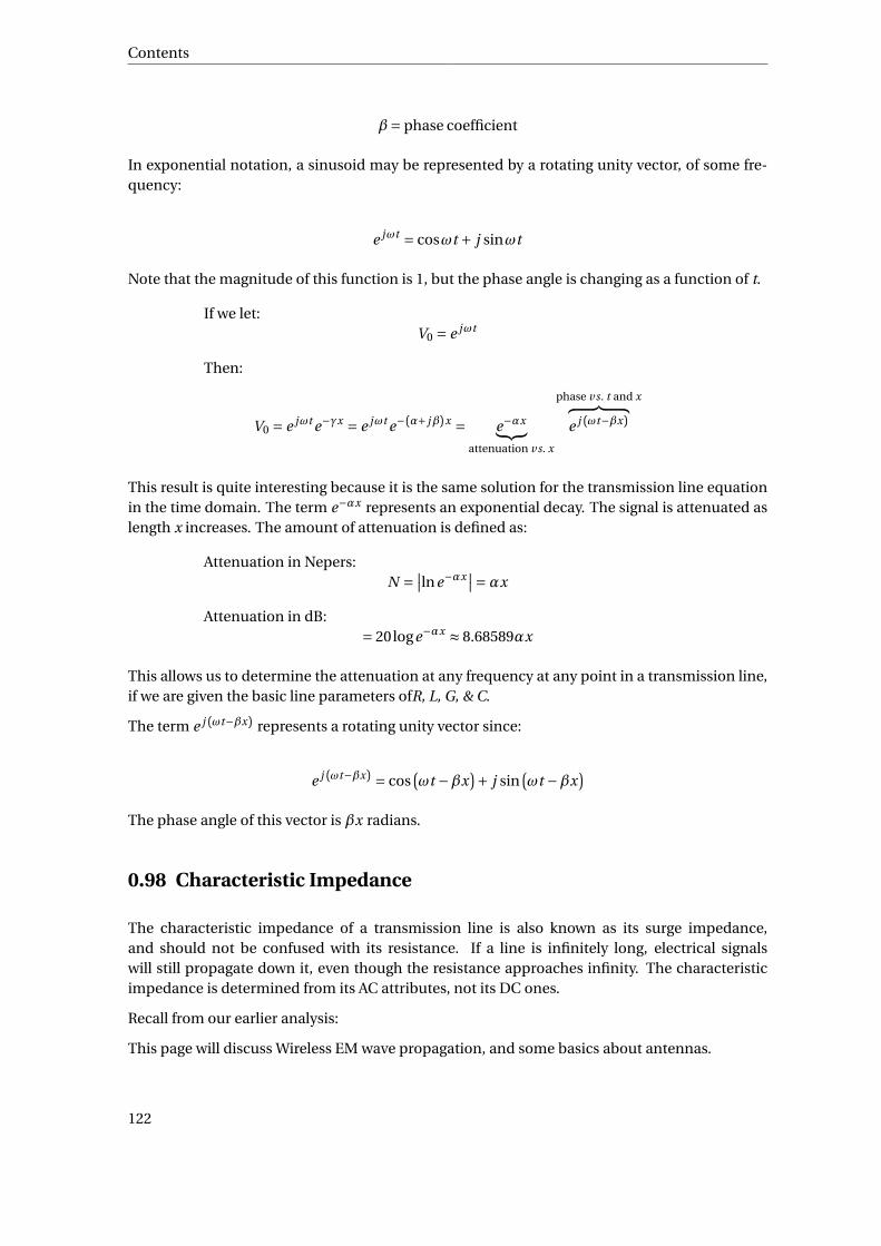
Contents

β= phase coefficient

In exponential notation, a sinusoid may be represented by a rotating unity vector, of some fre-quency:

e jωt = cosωt + j sinωt

Note that the magnitude of this function is 1, but the phase angle is changing as a function of t.

If we let:V0 = e jωt

Then:

V0 = e jωt e−γx = e jωt e−(α+ jβ)x = e−αx︸ ︷︷ ︸attenuation v s. x

phase v s. t and x︷ ︸︸ ︷e j(ωt−βx)

This result is quite interesting because it is the same solution for the transmission line equationin the time domain. The term e−αx represents an exponential decay. The signal is attenuated aslength x increases. The amount of attenuation is defined as:

Attenuation in Nepers:N = ∣∣lne−αx

∣∣=αx

Attenuation in dB:= 20loge−αx ≈ 8.68589αx

This allows us to determine the attenuation at any frequency at any point in a transmission line,if we are given the basic line parameters ofR, L, G, & C.

The term e j(ωt−βx) represents a rotating unity vector since:

e j(ωt−βx) = cos(ωt −βx

)+ j sin(ωt −βx

)The phase angle of this vector is βx radians.

0.98 Characteristic Impedance

The characteristic impedance of a transmission line is also known as its surge impedance,and should not be confused with its resistance. If a line is infinitely long, electrical signalswill still propagate down it, even though the resistance approaches infinity. The characteristicimpedance is determined from its AC attributes, not its DC ones.

Recall from our earlier analysis:

This page will discuss Wireless EM wave propagation, and some basics about antennas.

122

Isotropic Antennas

0.99 Isotropic Antennas

i Information

In communication we talk about ’antennas’; insects have ’antennae’

An isotropic antenna radiates it’s transmitted power equally in all directions. This is an idealmodel; all real antennas have at least some directionality associated with them. However, it ismathematically convenient, and good enough for most purposes.

i Information

A radio antenna is an example of an isotropic antenna

0.99.1 Power Flux Density

If the transmitted power is spread evenly across a sphere of radius R from the antenna, we canfind the power per unit area of that sphere, called the Power Flux Density using the Greek letter(capital phi) and the following formula:

Φ= PT

4πR2

Where PT is the total transmitted power of the signal.

0.99.2 Effective Area

The effective area of an antenna is the equivalent amount of area of transmission power, from anon-ideal isotropic antenna that appears to be the area from an ideal antenna. For instance, if ourantenna is non-ideal, and 1 meter squared of area can effectively be modeled as .5 meters squaredfrom an ideal antenna, then we can use the ideal number in our antenna. We can relate the actualarea and the effective area of our antenna using the antenna efficiency number, as follows:

η= Ae

A

The area of an ideal isotropic antenna can be calculated using the wavelength of the transmittedsignal as follows:

A = λ2

4π

123

Contents

0.99.3 Received Power

The amount of power that is actually received by a receiver placed at distance R from the isotropicantenna is denoted PR , and can be found with the following equation:

PR =ΦR Ae

Where ΦR is the power flux density at the distance R. If we plug in the formula for the effective areaof an ideal isotropic antenna into this equation, we get the following result:

PR = PT

(4πR/λ)2 = PT

LP

Where LP is the path-loss, and is defined as:

LP =(

4πR

λ

)2

The amount of power lost across freespace between two isotropic antenna (a transmitter and areceiver) depends on the wavelength of the transmitted signal.

0.100 Directional Antennas

A directional antenna, such as a parabolic antenna, attempts to radiate most of its power in thedirection of a known receiver.

i InformationA "satellite dish" is an example of a parabolic antenna

Here are some definitions that we need to know before we proceed:

Azimuth Angle:The Azimuth angle, often denoted with a (Greek lower-case Theta), is the anglethat the direct transmission makes with respect to a given reference angle (often the angle ofthe target receiver) when looking down on the antenna from above.

Elevation Angle:The elevation angle is the angle that the transmission direction makes with theground. Elevation angle is denoted with a (Greek lower-case phi)

0.100.1 Directivity

Given the above definitions, we can define the transmission gain of a directional antenna as a func-tion of and , assuming the same transmission power:

124

Link-Budget Analysis

GT (θ,φ) = Φθ, φ

Φi sotr opi c

0.100.2 Effective Area

The effective area of a parabolic antenna is given as such:

Ae = ηπD2

4

0.100.3 Transmit Gain

Gmax = 4πAe

λ2

If we are at the transmit antenna, and looking at the receiver, the angle that the transmission differsfrom the direction that we are looking is known as (Greek upper-case Psi), and we can find thetransmission gain as a function of this angle as follows:

G(Ψ) =(

2J1((πD/λ)si n(Ψ))

si n(Ψ)

)2 (λ

πD

)2

Where J1( ) denotes the first-order bessel function.

0.100.4 Friis Equation

The Friis Equation is used to relate several values together when using directional antennas:

PR = PT GT GR

LP

The Friis Equation is the fundamental basis for link-budget analysis.

0.101 Link-Budget Analysis

If we express all quantities from the Friis Equation in decibels, and divide both sides by the noise-density of the transmission medium, N0, we get the following equation:

C /N0 = E I RP −LP + (GR /Te )−k

Where C/N0 is the received carrier-to-noise ratio, and we can decompose N0 as follows:

125

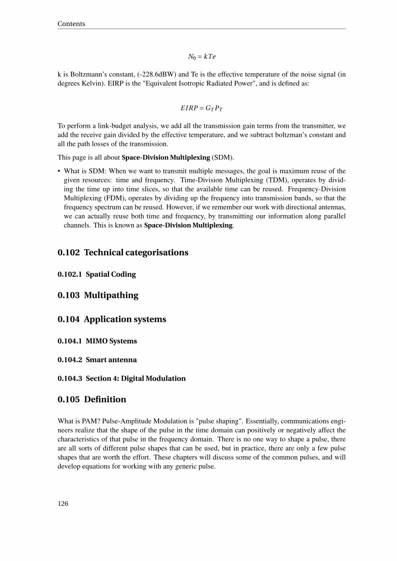
Contents

N0 = kTe

k is Boltzmann’s constant, (-228.6dBW) and Te is the effective temperature of the noise signal (indegrees Kelvin). EIRP is the "Equivalent Isotropic Radiated Power", and is defined as:

E I RP =GT PT

To perform a link-budget analysis, we add all the transmission gain terms from the transmitter, weadd the receive gain divided by the effective temperature, and we subtract boltzman’s constant andall the path losses of the transmission.

This page is all about Space-Division Multiplexing (SDM).

• What is SDM: When we want to transmit multiple messages, the goal is maximum reuse of thegiven resources: time and frequency. Time-Division Multiplexing (TDM), operates by divid-ing the time up into time slices, so that the available time can be reused. Frequency-DivisionMultiplexing (FDM), operates by dividing up the frequency into transmission bands, so that thefrequency spectrum can be reused. However, if we remember our work with directional antennas,we can actually reuse both time and frequency, by transmitting our information along parallelchannels. This is known as Space-Division Multiplexing.

0.102 Technical categorisations

0.102.1 Spatial Coding

0.103 Multipathing

0.104 Application systems

0.104.1 MIMO Systems

0.104.2 Smart antenna

0.104.3 Section 4: Digital Modulation

0.105 Definition

What is PAM? Pulse-Amplitude Modulation is "pulse shaping". Essentially, communications engi-neers realize that the shape of the pulse in the time domain can positively or negatively affect thecharacteristics of that pulse in the frequency domain. There is no one way to shape a pulse, thereare all sorts of different pulse shapes that can be used, but in practice, there are only a few pulseshapes that are worth the effort. These chapters will discuss some of the common pulses, and willdevelop equations for working with any generic pulse.

126

Square Wave

0.106 Square Wave

The most logical way to transmit a digital signal is through a stream of pulses. One distinct pulsefor a digital "1", and another distinct pulse for a digital "0". Intuitively, a square pulse will transmitthis data, and there are a number of different ways to transmit the data using

The square wave is a basic choice for transmitting digital data because it is easy to transmit, and isgenerally easy to receive. If we take the fourier transform of a square wave, we get a sinc function.A sinc function is a never-ending function, which means that a square wave in the time domainhas a very wide bandwidth. When using a square wave, there will always be a trade-off, becausehigh-frequency components of the square wave will be attenuated by the channel, and the resultantwaveform will be more prone to error on the other end.

0.106.1 Unipolar Square Wave

A unipolar square wave is a wave where a logical 1 is transmitted using a square pulse of height A.Then a logical 0 is transmitted with a 0 voltage.

0.106.2 Bipolar Square Wave

A bipolar square wave is a square wave where a 1 is transmitted with a pulse of height A/2, and a 0is transmitted with a pulse of -A/2.

0.107 Other pulses

It turns out that simply by changing the shape of the pulse (changing it away from a square wave),we can create a signal with better properties: lower bandwidth, lower error rate, etc... This sectionwill talk about a few different pulses.

0.108 Sinc

By the property of duality, however, we can see that if we have a sinc wave in the time domain, wewill have a square-shape in the frequency domain. This is an interesting result, because it means thatwe can transmit a sinc shape with definite bandwidth bounds, and it can travel through a channel inits entirety without being attenuated, or losing any harmonics!

0.109 Comparison

Here we will show a basic comparison between square pulses and sinc pulses:

Metric Square Pulse Sinc PulseBandwidth Large bandwidth Small bandwidth

127

Contents

Jitter Not susceptible to Jitter Very susceptible to JitterNoise Very susceptible to Noise Susceptible to NoiseISS Not affected by ISS Affected heavily by ISS

0.110 slew-rate-limited pulses

Most systems that use RS232, RS485, or high speed clocks use slew-rate-limited drivers. Some usedriver chips with integrated slew-rate limiting; other systems use digital driver chips that put sharpsquare pulses on their output pins, then an external slew-rate-limiting resistor40 between that outputpin and the rest of the system.

0.111 Raised-Cosine Rolloff

Sinc pulses use less bandwidth, but they are very susceptible to jitter. Conversely, Square pulseshave a large bandwidth, but are very resistant to jitter. The decision seems hopeless, but the intrepidcommunications engineer will try to find a 3rd option. The 3rd option is called the "Raised-CosineRolloff" pulse, and has the best characteristics of each wave. Raised Cosine Rolloff (RCR) pulsesare resistant to jitter, and at the same time have reasonably good bandwidth. Granted the bandwidthof an RCR pulse is wider than a sinc pulse, and the jitter resistance isn’t as good as with a squarewave, but this is a compromise, after all.

Pulse Bandwidth Jitter ResistanceRectangular rb/2 ExcellentSinc BadRCR Good

0.112 Binary symmetric pulses

A system uses binary symmetric pulses if it transmits only 2 kinds of pulse, s1 and s0, and s1(t) =-s0(t). In a symmetric case, our comparator circuits are very easy: If the correlator outputs a positivevalue, it’s a binary 1. If it outputs a negative value, it’s a binary 0.

40 SLEW-RATE-LIMITING RESISTOR ˆHTTP://MASSMIND.ORG/TECHREF/ELECTIPS.HTM#SERIES_RESISTOR

128

Asymmetric Pulses

0.113 Asymmetric Pulses

Asymmetric pulses are more difficult for many reasons:

1. The threshold where the comparator should test the value may not be zero2. The correlation receiver needs to correlate two different signals.3. The different pulses may have different power, and they may be different susceptible to noise.

0.114 Asymmetric Correlation Receiver

When asymmetric pulses are used, the receiver system must actually employ 2 coherent optimalreceivers, each one tuned to receive one of the pulses. When two coherent optimal receivers areused, the receiver that is outputting the highest voltage value at the end of time T has received it’spulse.

... why not employ only 1 coherent optimal receiver, tuned to receiver neither s0 nor s1, but insteadtuned to receive the difference (s1 - s0) ? ...

Some PAM systems, such as Ethernet 100BASE-T2, use PAM-5 ...

0.115 References

(PAM)

This page discusses the binary modulation schemes and "keying".

0.116 What is "Keying?"

Square waves, sinc waves, and raised-cosine rolloff waves are all well and good, but all of them havedrawbacks. If we use an optimal, matched filter, we can eliminate the effect of jitter, so frankly, whywould we consider square waves at all? Without jitter as a concern, it makes no sense to correct forjitter, or even take it into consideration. However, since the matched filter needs to look at individualsymbols, the transmitted signal can’t suffer from any intersymbol interference either. Therefore, wearen’t using the sinc pulse.

Since the raised-cosine roll-off wave suffers from both these problems (in smaller amounts, how-ever), we don’t want to use that pulse either.

So the question is, what other types of pulses can we send?

It turns out that if we use some of the techniques we have developed using analog signal modulation,and implement a sinusoidal carrier wave, we can create a signal with no inter-symbol interference,very low bandwidth, and no worries about jitter. Just like analog modulation, there are 3 aspects ofthe carrier wave that we can change: the amplitude, the frequency, and the phase angle. Instead of"modulation", we call these techniques keying techniques, because they are operating on a binary-number basis.

129

Contents

There is one important point to note before continuing with this discussion: Binary signals are notperiodic signals. Therefore, we cannot expect that a binary signal is going to have a discrete spectralike a periodic squarewave will have. For this reason, the spectral components of binary data arecontinuous spectra.

0.117 Amplitude Shift Keying

In an ASK system, we are changing the amplitude of the sine wave to transmit digitial data. Wehave the following cases:

• Binary 1: A1 sin( fc t )• Binary 0: A0 sin( fc t )

The simplest modulation scheme sets A0 = 0V (turning the transmitter off), and setting A1 = +5V(any random non-zero number turns the transmitter on). This special case of ASK is called OOK(On-Off keying). Morse code uses OOK.

Another common special case of ASK sets A1 to some positive number, and A0 to the correspondingnegative number A0 = -A1. We will mention this case again later.

In ASK, we have the following equation:

a(t )sin(ωt )

by the principal of duality, multiplication in the time domain becomes convolution in the frequencydomain, and vice-versa. Therefore, our frequency spectrum will have the following equation:

A( jω)∗δ(t −ω)

where the impulse function is the fourier-transform of the sinusoid, centered at the frequency ofthe wave. the value for A is going to be a sinc wave, with a width dependant on the bitrate. Weremember from the SIGNALS AND SYSTEMS41 book that convolution of a signal with an impulseis that signal centered where the impulse was centered. Therefore, we know now that the frequencydomain shape of this curve is a sinc wave centered at the carrier frequency.

0.118 Frequency Shift Keying

In Frequency Shift Keying (FSK), we can logically assume that the parameter that we will bechanging is the frequency of the sine wave. FSK is unique among the different keying methods inthat data is never transmitted at the carrier frequency, but is instead transmitted at a certain offsetfrom the carrier frequency. If we have a carrier frequency of fc , and a frequency offset of ∆ f , wecan transmit binary values as such:

• Binary 1: A sin(( fc +∆ f )t )

41 HTTP://EN.WIKIBOOKS.ORG/WIKI/SIGNALS%20AND%20SYSTEMS

130

Phase Shift Keying

• Binary 0: A sin(( fc −∆ f )t )

Similar to ASK, we have FSK, which uses 2 different frequencies to transmit data. For now wewill call them ω1,ω2. Using the same logic that we used above, the fourier representations of thesewaves will be (respectively):

A1( jω)∗δ(t −ω1)

A0( jω)∗δ(t −ω2)

With one sinc wave centered at the first frequency, and one sinc wave centered at the second fre-quency. Notice that A1 and A0 are the half-square waves associated with the 1s and the 0s, respec-tively. These will be described later.

0.118.1 Error Rate

The BER of coherent QPSK in the presence of gaussian and Rayleigh noise is as follows:

| border=1

|- | Gaussian Noise || Rayleigh Fading |- | 12 erfc

(√EbN0

)| 1

2

(1−

√γ0

2+γ0

)|

0.119 Phase Shift Keying

PSK systems are slightly different then ASK and FSK systems, and because of this difference, wecan exploit an interesting little trick of trigonometry. PSK is when we vary the phase angle of thewave to transmit different bits. For instance:

• Binary 1: A sin( fc t +φ1)• Binary 0: A sin( fc t +φ0)

If we evenly space them out around the unit-circle, we can give ourselves the following nice values:

• Binary 1: A sin( fc t +0)• Binary 0: A sin( fc t +π)

Now, according to trigonometry, we have the following identity:

sin( fc t +π) =−sin( fc t )

So in general, our equations for each signal (s) is given by:

• s1(t ) = A sin( fc t )• s0(t ) =−A sin( fc t )

Which looks awfully like an ASK signal. Therefore, we can show that the spectrum of a PSK signalis the same as the spectrum of an ASK signal.

There are two commonally used forms of Phase Shift keying Modulation:

131

Contents

Binary Phase Shift Keying (BPSK)

Quadrature Phase Shift Keying (QPSK)

Binary Phase Shift keying is set out above.

0.119.1 QPSK

Quadrature Phase Shift Keying utilises the fact that a cosine wave is in quadrature to a sine wave,allowing 2 bits to be simultaneously represented.

• Binary 11: A sin( fc t +0)+cos( fc +π/2)• Binary 10: A sin( fc t +0)+cos( fc −π/2)• Binary 01: A sin( fc t +π)++cos( fc +π/2)• Binary 00: A sin( fc t +π)++cos( fc −π/2)

QPSK has the advantage over BPSK of requiring half the transmission band width for the same datarate, and error probability.

0.119.2 Error Rate

The BER of coherent BPSK in the presence of gaussian and Rayleigh noise is as follows:

| border=1

|- | Gaussian Noise || Rayleigh Fading |- | 12 erfc

(√EbN0

)| 1

2

(1−

√γ0

1+γ0

)|

0.120 Binary Transmitters

0.121 Binary Receivers

Now what if try to cram more information into a single bittime? If we take 2 bits at a time, andarrange them together, we can assign each set of 2 bits to a different symbol, and then we cantransmit the different symbols.

0.122 Pronunciation

First off, "M-ary" is not pronounced like the female name "mary". If you say "mary" to a boardroomfilled with engineers, they will laugh at you, and your boss will politely tell you later to start cleaningup your desk. "M-ary" is pronounced like "em airy".

132

Example: 4-ASK

0.123 Example: 4-ASK

Let us use the following scheme:

• "00" = +5V• "01" = +1.66V• "10" = -1.66V• "11" = -5V

we can see now that we can transmit data twice as fast using this scheme, although we need tohave a more complicated receiver, that can decide between 4 different pulses (instead of 2 differentpulses, like we have been using).

0.124 Bits Per Symbol

All popular communication systems transmit an integer number of bits per symbol. We can relatethe number of bits ("k") and the number of different symbols ("m") with the following equation:

m = 2k

This causes the number of symbols to be a power of two.

With M-ary modulation techniques, the "symbols per second" rate can be much slower than the"bits per second" data rate.

0.125 QPSK

0.126 CPFSK (MSK)

[MSK]minimum shift keying

0.127 DPSK

0.128 For further reading

• WIKIPEDIA:CONSTELLATION_DIAGRAM42

• WIKIPEDIA:QUADRATURE AMPLITUDE MODULATION43

42 HTTP://EN.WIKIPEDIA.ORG/WIKI/CONSTELLATION_DIAGRAM43 HTTP://EN.WIKIPEDIA.ORG/WIKI/QUADRATURE%20AMPLITUDE%20MODULATION

133

Contents

The quadrature amplitude modulation (QAM) system of modulation is the most popular M-ARY

SCHEME44.

0.129 Definition

Consider the case of a system with two carrier waves instead of a single carrier wave as we haveconsidered with modulation schemes so far. One is a sine wave, and the other is a cosine wave ofthe same frequency. Since these two waves are orthogonal we can use them simultaneously in asingle channel without losing the information of either. If both waves have the same frequency f wecan write out the equation for a generic symbol, s:

s(t ) = Ak sin( f t )+Bk cos( f t )

In this way, we can create multiple symbols by simply changing the values of A and B. This equationcan be broken up into two parts:

• Ak sin( f t ) Which is called the "in-phase" component of the equation.• Bk cos( f t ) Which is called the "quadrature" component of the equation.

An equation which is written as a sum of a sine plus a cosine is said to be in "quadrature form". Ifwe combine the two components into a single waveform as such:

s(t ) =√

A2k +B 2

k cos( f t + tan−1(Bk /Ak ))

This form is called the "Polar Form" of the equation.

i Information56K modems and Digital TV use QAM

0.130 Constellation Plots

If we make a graph with the X axis being the values for A, and the Y axis being the values for B,we get what is called a Constellation Plot. These plots are called constellation plots due to thesimiliarity in shape and layout with astronomical star charts. The A and B values for each symbolare plotted (the "stars") and various measurements between them are used to determine informationfrom the system. On a constellation plot, we can see a number of rules:

1. The further apart the points are on the constellation plot, the less likely they are to be mistakenfor each other in the presence of noise.

2. The closer the points are to the origin, the less power it takes to send.

44 HTTP://EN.WIKIBOOKS.ORG/WIKI/COMMUNICATION%20SYSTEMS%2FM-ARY%20MODULATION%20SCHEMES%20

134

Benefits of QAM

3. The more points there are, the faster the data rate (bit rate) at a fixed symbol rate (moresymbols)

4. The fewer points there are, the simpler and cheaper the hardware necessary to distinguishbetween them (fewer symbols, fewer thresholds in the receiver).

For these reasons there is no single "best" constellation plot, but it is up to the engineer to pickthe points that are best for the system. In other words, trade offs need to be made between speed,performance, and cost of hardware. These tradeoffs can be made by placing the constellation pointsat different locations on the constellation plot.

0.131 Benefits of QAM

Increase the efficiency of transmission by utilising both amplitude and phase variations.

Reducing or eliminating intermodulation interference caused by a continuous carrier near the mod-ulation sidebands.

0.132 For further reading

QUADRATURE AMPLITUDE MODULATION45 CONSTELLATION DIAGRAM46

The quadrature amplitude modulation (QAM) system of modulation is the most popular M-aryscheme.

0.133 Definition

Let us say that we have 2 carrier waves. One is a sine wave, and the other is a cosine wave. Sincethese two waves are orthogonal, we can use them simultaneously, without losing the information ofeither. If both waves have the same frequency, f, we can write out the equation for a generic symbol,s:

s(t ) = Ak sin( f t )+Bk cos( f t )

In this way, we can create multiple symbols by simply changing the values of A and B. This equationcan be broken up into two parts:

• Ak sin( f t ) Which is called the "in-phase" component of the equation.• Bk cos( f t ) Which is called the "quadrature" component of the equation.

An equation which is written as a sum of a sine plus a cosine is said to be in "quadrature form". Ifwe combine the two components into a single waveform as such:

45 HTTP://EN.WIKIPEDIA.ORG/WIKI/QUADRATURE%20AMPLITUDE%20MODULATION46 HTTP://EN.WIKIPEDIA.ORG/WIKI/CONSTELLATION%20DIAGRAM

135

Contents

s(t ) =√

A2k +B 2

k cos( f t + tan−1(Bk /Ak ))

This form is called the "Polar Form" of the equation.

i Information56K modems and Digital TV use QAM

0.134 Constellation Plots

If we make a graph with the X axis being the values for A, and the Y axis being the values for B, weget what is called a "Constellation Plot". If A and B have discrete values, then the constellation plotwill show dots at points that correspond to values for A and B coordinates. It is called a constellationplot because the layout of the different points can look very similar to the layout of stars in the sky.

On a constellation plot, we can see a number of points:

1. The further apart the points are, the less likely they are to be mixed up2. The closer the points are to the origin, the less power it takes to send.

1. The more points there are, the faster the data rate (bit rate) at a fixed symbol rate.2. The fewer points there are, the simpler and cheaper the hardware necessary to distinguish

between them.

For these two reasons, there is no single "best" constellation plot, but it is up to the engineer to pickthe points that are best for the system. By placing the points manually, the engineer is able to maketrade-offs between the power of the system, and the number of bits per symbol (and therefore thebitrate).

0.135 Benefits of QAM

0.136 For further reading

QUADRATURE AMPLITUDE MODULATION47 CONSTELLATION DIAGRAM48 (QAM)

1. REDIRECT COMMUNICATION SYSTEMS/NONCOHERENT RECEIVERS49

47 HTTP://EN.WIKIPEDIA.ORG/WIKI/QUADRATURE%20AMPLITUDE%20MODULATION48 HTTP://EN.WIKIPEDIA.ORG/WIKI/CONSTELLATION%20DIAGRAM49 HTTP://EN.WIKIBOOKS.ORG/WIKI/COMMUNICATION%20SYSTEMS%2FNONCOHERENT%

20RECEIVERS

136

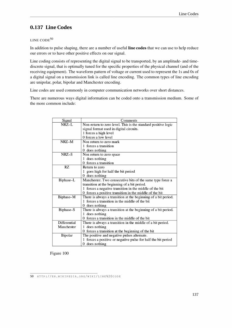
Line Codes

0.137 Line Codes

LINE CODE50

In addition to pulse shaping, there are a number of useful line codes that we can use to help reduceour errors or to have other positive effects on our signal.

Line coding consists of representing the digital signal to be transported, by an amplitude- and time-discrete signal, that is optimally tuned for the specific properties of the physical channel (and of thereceiving equipment). The waveform pattern of voltage or current used to represent the 1s and 0s ofa digital signal on a transmission link is called line encoding. The common types of line encodingare unipolar, polar, bipolar and Manchester encoding.

Line codes are used commonly in computer communication networks over short distances.

There are numerous ways digital information can be coded onto a transmission medium. Some ofthe more common include:

Figure 100

50 HTTP://EN.WIKIPEDIA.ORG/WIKI/LINE%20CODE

137

Contents

| style="border-collapse:collapse;background:white;" cellpadding=5pxalign=left width=72%

|+ Common line codes |- style="font-weight:bold; text-align:center;" ! width=20% style=" bor-der:1px solid gray;"|Signal ! width=80% style=" border:1px solid gray;"|Comments |- valign=top| style="border:1px solid gray; text-align:center;"| NRZ-L | style="border:1px solid gray;"| Non-return to zero level. This is the standard positive logic signal format used in digital circuits.

1 forces a high level

0 forces a low level |- valign=top | style="border:1px solid gray; text-align:center;"| NRZ-M |style="border:1px solid gray;"| Non-return to zero mark.

1 forces a transition

0 does nothing |- valign=top | style="border:1px solid gray; text-align:center;"| NRZ-S |style="border:1px solid gray;"| Non-return to zero space.

1 does nothing

0 forces a transition |- valign=top | style="border:1px solid gray; text-align:center;"| RZ |style="border:1px solid gray;"| Return to zero.

1 goes high for half the bit period

0 does nothing |- valign=top | style="border:1px solid gray; text-align:center;"| Biphase-L |style="border:1px solid gray;"| Manchester. Two consecutive bits of the same type force a transi-tion at the beginning of a bit period.

1 forces a negative transition in the middle of the bit

0 forces a positive transition in the middle of the bit |- valign=top | style="border:1px solid gray;text-align:center;"| Biphase-M | style="border:1px solid gray;"| There is always a transition at thebeginning of a bit period. 1 forces a transition in the middle of the bit. 0 does nothing. |- valign=top| style="border:1px solid gray; text-align:center;"| Biphase-S | style="border:1px solid gray;"| Thereis always a transition at the beginning of a bit period. 1 does nothing

0 forces a transition in the middle of the bit. |- valign=top | style="border:1px solid gray; text-align:center;"| Differential Manchester | style="border:1px solid gray;"| There is always a transitionin the middle of a bit period.

138

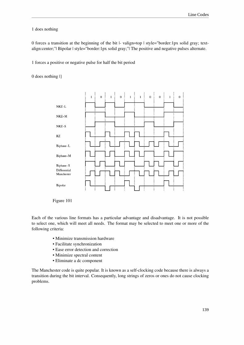
Line Codes

1 does nothing

0 forces a transition at the beginning of the bit |- valign=top | style="border:1px solid gray; text-align:center;"| Bipolar | style="border:1px solid gray;"| The positive and negative pulses alternate.

1 forces a positive or negative pulse for half the bit period

0 does nothing |

Figure 101

Each of the various line formats has a particular advantage and disadvantage. It is not possibleto select one, which will meet all needs. The format may be selected to meet one or more of thefollowing criteria:

• Minimize transmission hardware• Facilitate synchronization• Ease error detection and correction• Minimize spectral content• Eliminate a dc component

The Manchester code is quite popular. It is known as a self-clocking code because there is always atransition during the bit interval. Consequently, long strings of zeros or ones do not cause clockingproblems.

139

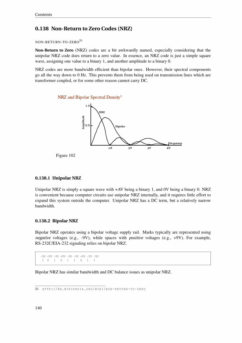
Contents

0.138 Non-Return to Zero Codes (NRZ)

NON-RETURN-TO-ZERO51

Non-Return to Zero (NRZ) codes are a bit awkwardly named, especially considering that theunipolar NRZ code does return to a zero value. In essence, an NRZ code is just a simple squarewave, assigning one value to a binary 1, and another amplitude to a binary 0.

NRZ codes are more bandwidth efficient than bipolar ones. However, their spectral componentsgo all the way down to 0 Hz. This prevents them from being used on transmission lines which aretransformer coupled, or for some other reason cannot carry DC.

Figure 102

0.138.1 Unipolar NRZ

Unipolar NRZ is simply a square wave with +AV being a binary 1, and 0V being a binary 0. NRZis convenient because computer circuits use unipolar NRZ internally, and it requires little effort toexpand this system outside the computer. Unipolar NRZ has a DC term, but a relatively narrowbandwidth.

0.138.2 Bipolar NRZ

Bipolar NRZ operates using a bipolar voltage supply rail. Marks typically are represented usingnegative voltages (e.g., -9V), while spaces with positive voltages (e.g., +9V). For example,RS-232C/EIA-232 signaling relies on bipolar NRZ.

-5V +5V -5V +5V -5V -5V +5V -5V -5V1 0 1 0 1 1 0 1 1

Bipolar NRZ has similar bandwidth and DC balance issues as unipolar NRZ.

51 HTTP://EN.WIKIPEDIA.ORG/WIKI/NON-RETURN-TO-ZERO

140

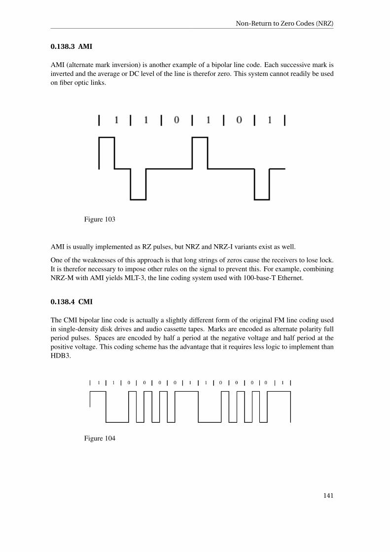
Non-Return to Zero Codes (NRZ)

0.138.3 AMI

AMI (alternate mark inversion) is another example of a bipolar line code. Each successive mark isinverted and the average or DC level of the line is therefor zero. This system cannot readily be usedon fiber optic links.

Figure 103

AMI is usually implemented as RZ pulses, but NRZ and NRZ-I variants exist as well.

One of the weaknesses of this approach is that long strings of zeros cause the receivers to lose lock.It is therefor necessary to impose other rules on the signal to prevent this. For example, combiningNRZ-M with AMI yields MLT-3, the line coding system used with 100-base-T Ethernet.

0.138.4 CMI

The CMI bipolar line code is actually a slightly different form of the original FM line coding usedin single-density disk drives and audio cassette tapes. Marks are encoded as alternate polarity fullperiod pulses. Spaces are encoded by half a period at the negative voltage and half period at thepositive voltage. This coding scheme has the advantage that it requires less logic to implement thanHDB3.

Figure 104

141

Contents

0.139 Manchester

MANCHESTER CODE52

Manchester codes were an invention that allows for timing information to be sent along with thedata. In an NRZ code, if there is a long stream of ones or zeros, the receiver could conceivablysuffer so much compound jitter that it would either lose or gain an entire bit time, and then be out ofsync with the transmitter. This is because a long stream of 1s or 0s would not "change state" at all,but instead would simply stay at a single value. Manchester codes say that every single bittime willhave a transition in the middle of the bit time, so that a receiver could find that transition, and "lockon" to the signal again, if it started to stray away from center. Because there are more transitions,however, manchester codes also require the highest bandwidth of all the line codes.

i InformationEthernet LAN uses manchester codes

0.140 Differential Codes

Some communication channels (such as phase-modulated sine waves and differential twisted pairs)have the characteristic that transitions between the 2 symbols used can be easily distinguished, butwhen first starting to receive it is difficult to tell which of the 2 states it is in. For example, full-speedUSB uses a twisted pair and transmits +3.3 V on one line and 0 V on the other line for "1", but 0 Von the one line and +3.3 V on the other line for "0". Because some cables have an extra half-twist inthem, it is impossible for a device that was just plugged in to tell whether the symbol it is currentlyreceiving is a "1" or a "0".

Differential codes still work, not even noticing when the 2 wires get switched.

Differential codes, in general, look exactly the same on a oscilloscope or spectrum analyzer as thenon-differential code they are based on, and so use exactly the same bandwidth and have exactlythe same bitrate.

Differential codes that work when the 2 wires get switched include:

• Differential Manchester encoding -- based on Manchester encoding• Non-Return-to-Zero Inverted (NRZI) -- based on non-return-to-zero (NRZ)

(A few non-differential codes also work even when the 2 wires get switched -- such as bipolarencoding, and MLT-3 encoding).

52 HTTP://EN.WIKIPEDIA.ORG/WIKI/MANCHESTER%20CODE

142

further reading

0.140.1 Differential NRZ

0.140.2 Differential Manchester

0.141 Comparison

Code Bandwidth Timing DC valueUnipolar NRZ Low bandwidth No timing informa-

tionHigh DC compo-nent

Bipolar NRZ Lower bandwidth No timing informa-tion

No DC component

Differential NRZ Lower bandwidth No timing informa-tion

Little or no DCcomponent

Manchester High bandwidth Good clock recov-ery

No DC component

Differential Manch-ester

Moderate band-width

Good clock recov-ery

No DC Component

0.142 further reading

• WIKIPEDIA:DIFFERENTIAL CODING53

0.142.1 Section 5: Analog Networks

1. REDIRECT COMMUNICATION NETWORKS/CIRCUIT SWITCHING NETWORKS54

1. REDIRECT COMMUNICATION NETWORKS/CABLE TELEVISION NETWORK55

1. REDIRECT COMMUNICATION NETWORKS/RADIO COMMUNICATIONS56

0.142.2 Section 6: Digital Networks

1. REDIRECT COMMUNICATION NETWORKS/PARALLEL VS SERIAL57

1. REDIRECT COMMUNICATION NETWORKS/OSI REFERENCE MODEL58

53 HTTP://EN.WIKIPEDIA.ORG/WIKI/DIFFERENTIAL%20CODING54 HTTP://EN.WIKIBOOKS.ORG/WIKI/COMMUNICATION%20NETWORKS%2FCIRCUIT%20SWITCHING%

20NETWORKS55 HTTP://EN.WIKIBOOKS.ORG/WIKI/COMMUNICATION%20NETWORKS%2FCABLE%20TELEVISION%

20NETWORK56 HTTP://EN.WIKIBOOKS.ORG/WIKI/COMMUNICATION%20NETWORKS%2FRADIO%

20COMMUNICATIONS57 HTTP://EN.WIKIBOOKS.ORG/WIKI/COMMUNICATION%20NETWORKS%2FPARALLEL%20VS%

20SERIAL58 HTTP://EN.WIKIBOOKS.ORG/WIKI/COMMUNICATION%20NETWORKS%2FOSI%20REFERENCE%

20MODEL

143

Contents

1. REDIRECT COMMUNICATION NETWORKS/CHANNELS59

1. REDIRECT COMMUNICATION NETWORKS/INTERNET60

1. REDIRECT COMMUNICATION NETWORKS/ETHERNET61 (IEEE 802.3)

1. REDIRECT COMMUNICATION NETWORKS/WIRELESS INTERNET62

0.142.3 Section 7: Hybrid Networks

1. REDIRECT COMMUNICATION NETWORKS/ANALOG AND DIGITAL TV63

1. REDIRECT COMMUNICATION NETWORKS/ANALOG AND DIGITAL TELEPHONY64

0.142.4 Section 8: Advanced Internet

ARP Protocol and ARPANET Internet Backbone (Fiber Optics and SONET, ATM Networks)

1. REDIRECT COMMUNICATION NETWORKS/BERKELEY SOCKET API65

DNS

1. REDIRECT COMMUNICATION NETWORKS/IP PROTOCOL AND ICMP66

1. REDIRECT COMMUNICATION NETWORKS/TCP AND UDP PROTOCOLS67

1. REDIRECT COMMUNICATION NETWORKS/HTTP PROTOCOL68

FILE TRANSFER PROTOCOL69 File Transfer Protocol (FTP) is a standard network protocol used toexchange and manipulate files over a TCP/IP based network, such as the INTERNET70. FTP is builton a client-server architecture and utilizes separate control and data connections between the clientand server applications. FTP is also often used as an application component to automatically transferfiles for program internal functions. FTP can be used with user-based password authentication orwith anonymous user access.

59 HTTP://EN.WIKIBOOKS.ORG/WIKI/COMMUNICATION%20NETWORKS%2FCHANNELS60 HTTP://EN.WIKIBOOKS.ORG/WIKI/COMMUNICATION%20NETWORKS%2FINTERNET61 HTTP://EN.WIKIBOOKS.ORG/WIKI/COMMUNICATION%20NETWORKS%2FETHERNET62 HTTP://EN.WIKIBOOKS.ORG/WIKI/COMMUNICATION%20NETWORKS%2FWIRELESS%20INTERNET63 HTTP://EN.WIKIBOOKS.ORG/WIKI/COMMUNICATION%20NETWORKS%2FANALOG%20AND%

20DIGITAL%20TV64 HTTP://EN.WIKIBOOKS.ORG/WIKI/COMMUNICATION%20NETWORKS%2FANALOG%20AND%

20DIGITAL%20TELEPHONY65 HTTP://EN.WIKIBOOKS.ORG/WIKI/COMMUNICATION%20NETWORKS%2FBERKELEY%20SOCKET%

20API66 HTTP://EN.WIKIBOOKS.ORG/WIKI/COMMUNICATION%20NETWORKS%2FIP%20PROTOCOL%20AND%

20ICMP67 HTTP://EN.WIKIBOOKS.ORG/WIKI/COMMUNICATION%20NETWORKS%2FTCP%20AND%20UDP%

20PROTOCOLS68 HTTP://EN.WIKIBOOKS.ORG/WIKI/COMMUNICATION%20NETWORKS%2FHTTP%20PROTOCOL69 HTTP://EN.WIKIPEDIA.ORG/WIKI/FILE%20TRANSFER%20PROTOCOL70 HTTP://EN.WIKIBOOKS.ORG/WIKI/INTERNET

144

Purpose

0.143 Purpose

Objectives of FTP, as outlined by its RFC, are:

• To promote sharing of files (computer programs and/or data).• To encourage indirect or implicit use of remote computers.• To shield a user from variations in file storage systems among different hosts.• To transfer data reliably, and efficiently.

0.144 Connection methods

FTP runs over the Transmission Control Protocol (TCP). Usually FTP servers listen on the well-known port number 21 (IANA-reserved) for incoming connections from clients. A connectionto this port from the FTP client forms the control stream on which commands are passed to theFTP server and responses are collected. FTP uses out-of-band control; it opens dedicated dataconnections on other port numbers. The parameters for the data streams depend on the specificallyrequested transport mode. Data connections usually use port number 20.

In active mode, the FTP client opens a dynamic port, sends the FTP server the dynamic port numberon which it is listening over the control stream and waits for a connection from the FTP server. Whenthe FTP server initiates the data connection to the FTP client it binds the source port to port 20 onthe FTP server.

In order to use active mode, the client sends a PORT command, with the IP and port as argument.The format for the IP and port is "h1,h2,h3,h4,p1,p2". Each field is a decimal representation of 8bits of the host IP, followed by the chosen data port. For example, a client with an IP of 192.168.0.1,listening on port 49154 for the data connection will send the command "PORT 192,168,0,1,192,2".The port fields should be interpreted as p1×256 + p2 = port, or, in this example, 192×256 + 2 =49154.

In passive mode, the FTP server opens a dynamic port, sends the FTP client the server’s IP addressto connect to and the port on which it is listening (a 16-bit value broken into a high and low byte,as explained above) over the control stream and waits for a connection from the FTP client. In thiscase, the FTP client binds the source port of the connection to a dynamic port.

To use passive mode, the client sends the PASV command to which the server would reply withsomething similar to "227 Entering Passive Mode (127,0,0,1,192,52)". The syntax of the IP addressand port are the same as for the argument to the PORT command.

In extended passive mode, the FTP server operates exactly the same as passive mode, however itonly transmits the port number (not broken into high and low bytes) and the client is to assume thatit connects to the same IP address that was originally connected to.

While data is being transferred via the data stream, the control stream sits idle. This can causeproblems with large data transfers through firewalls which time out sessions after lengthy periods ofidleness. While the file may well be successfully transferred, the control session can be disconnectedby the firewall, causing an error to be generated.

The FTP protocol supports resuming of interrupted downloads using the REST command. Theclient passes the number of bytes it has already received as argument to the REST command and

145

Contents

restarts the transfer. In some commandline clients for example, there is an often-ignored but valu-able command, "reget" (meaning "get again"), that will cause an interrupted "get" command to becontinued, hopefully to completion, after a communications interruption.

Resuming uploads is not as easy. Although the FTP protocol supports the APPE command toappend data to a file on the server, the client does not know the exact position at which a transfer gotinterrupted. It has to obtain the size of the file some other way, for example over a directory listingor using the SIZE command.

In ASCII mode (see below), resuming transfers can be troublesome if client and server use differentend of line characters.

0.145 Data format

While transferring data over the network, several data representations can be used. The two mostcommon transfer modes are:

• ASCII mode• Binary mode: In "Binary mode", the sending machine sends each file byte for byte and as such

the recipient stores the bytestream as it receives it. (The FTP standard calls this "IMAGE" or "I"mode)

In ASCII mode, any form of data that is not plain text will be corrupted. When a file is sent usingan ASCII-type transfer, the individual letters, numbers, and characters are sent using their ASCIIcharacter codes. The receiving machine saves these in a text file in the appropriate format (forexample, a Unix machine saves it in a Unix format, a Windows machine saves it in a Windowsformat). Hence if an ASCII transfer is used it can be assumed plain text is sent, which is stored bythe receiving computer in its own format. Translating between text formats might entail substitutingthe end of line and end of file characters used on the source platform with those on the destinationplatform, e.g. a Windows machine receiving a file from a Unix machine will replace the line feedswith carriage return-line feed pairs. It might also involve translating characters; for example, whentransferring from an IBM mainframe to a system using ASCII, EBCDIC characters used on themainframe will be translated to their ASCII equivalents, and when transferring from the systemusing ASCII to the mainframe, ASCII characters will be translated to their EBCDIC equivalents.

By default, most FTP clients use ASCII mode. Some clients try to determine the required transfer-mode by inspecting the file’s name or contents, or by determining whether the server is running anoperating system with the same text file format.

The FTP specifications also list the following transfer modes:

• EBCDIC mode - this transfers bytes, except they are encoded in EBCDIC rather than ASCII.Thus, for example, the ASCII mode server

• Local mode - this is designed for use with systems that are word-oriented rather than byte-oriented. For example mode "L 36" can be used to transfer binary data between two 36-bitmachines. In L mode, the words are packed into bytes rather than being padded. Some FTPservers accept "L 8" as being equivalent to "I".

In practice, these additional transfer modes are rarely used. They are however still used by somelegacy mainframe systems.

146

FTP return codes

The text (ASCII/EBCDIC) modes can also be qualified with the type of carriage control used (e.g.TELNET NVT carriage control, ASA carriage control), although that is rarely used nowadays.

Note that the terminology "mode" is technically incorrect, although commonly used by FTP clients."MODE" in RFC 959 refers to the format of the protocol data stream (STREAM, BLOCK or COM-PRESSED), as opposed to the format of the underlying file. What is commonly called "mode" isactually the "TYPE", which specifies the format of the file rather than the data stream. FTP also sup-ports specification of the file structure ("STRU"), which can be either FILE (stream-oriented files),RECORD (record-oriented files) or PAGE (special type designed for use with TENEX). PAGESTRU is not really useful for non-TENEX systems, and RFC 1123 section 4.1.2.3 recommends thatit not be implemented.

0.146 FTP return codes

FTP server return codes indicate their status by the digits within them. A brief explanation of variousdigits’ meanings are given below:

• 1xx: Positive Preliminary reply. The action requested is being initiated but there will be anotherreply before it begins.

• 2xx: Positive Completion reply. The action requested has been completed. The client may nowissue a new command.

• 3xx: Positive Intermediate reply. The command was successful, but a further command is requiredbefore the server can act upon the request.

• 4xx: Transient Negative Completion reply. The command was not successful, but the client isfree to try the command again as the failure is only temporary.

• 5xx: Permanent Negative Completion reply. The command was not successful and the clientshould not attempt to repeat it again.

• x0x: The failure was due to a syntax error.• x1x: This response is a reply to a request for information.• x2x: This response is a reply relating to connection information.• x3x: This response is a reply relating to accounting and authorization.• x4x: Unspecified as yet• x5x: These responses indicate the status of the Server file system vis-a-vis the requested transfer

or other file system action.

0.147 Anonymous FTP

A host that provides an FTP service may additionally provide anonymous FTP access. Users typ-ically login to the service with an ’anonymous’ account when prompted for user name. Althoughusers are commonly asked to send their email address in lieu of a password, little to no verificationis actually performed on the supplied data.

As modern FTP clients typically hide the anonymous login process from the user, the ftp clientwill supply dummy data as the password (since the user’s email address may not be known to theapplication). For example, the following ftp user agents specify the listed passwords for anonymouslogins:

147

Contents

• MOZILLA FIREFOX71 (3.0.7) — mozilla@example.com• KDE72 Konqueror (3.5) — anonymous@• wget (1.10.2) — -wget@• lftp (3.4.4) — lftp@

0.148 Commands

Enter ftp /? in Windows, or ftp --help in Unix, to get the command parameters.

Once connected to a server, type help to display the different possible commands.

To manipulate the files with the mouth, download a good FTP client which will do the interface (forexample THIS FILEZILLA DOESN’T NEED ANY INSTALLATION73).

1. REDIRECT COMMUNICATION NETWORKS/ROUTING74

0.148.1 Section 9: Coding and Security

1. REDIRECT DATA CODING THEORY/TRANSMISSION CODES75

1. REDIRECT DATA CODING THEORY/SPECTRUM SPREADING76

1. REDIRECT DATA CODING THEORY/DATA COMPRESSION77

1. REDIRECT DATA CODING THEORY/HAMMING CODES78

Network Security (HTTPS and SSN) WEP MD5 Checksum DES and RSA

0.148.2 Appendices

The 802 portion of the IEEE is responsible for publishing standards on a number of different proto-cols. Any chapter with a note such as (IEEE 802.3) is referring to the group below that has publishedthe currently accepted standard for that topic.

Working Group Task Status802.1 Higher Layer LAN Proto-

cols Working GroupActive

802.2 Logical Link Control Work-ing Group

Inactive

802.3 Ethernet Working Group Active802.4 Token Bus Working Group Disbanded

71 HTTP://EN.WIKIBOOKS.ORG/WIKI/MOZILLA%20FIREFOX72 HTTP://EN.WIKIBOOKS.ORG/WIKI/KDE73 HTTP://PORTABLEAPPS.COM/APPS/INTERNET/FILEZILLA_PORTABLE74 HTTP://EN.WIKIBOOKS.ORG/WIKI/COMMUNICATION%20NETWORKS%2FROUTING75 HTTP://EN.WIKIBOOKS.ORG/WIKI/DATA%20CODING%20THEORY%2FTRANSMISSION%20CODES76 HTTP://EN.WIKIBOOKS.ORG/WIKI/DATA%20CODING%20THEORY%2FSPECTRUM%20SPREADING77 HTTP://EN.WIKIBOOKS.ORG/WIKI/DATA%20CODING%20THEORY%2FDATA%20COMPRESSION78 HTTP://EN.WIKIBOOKS.ORG/WIKI/DATA%20CODING%20THEORY%2FHAMMING%20CODES

148

Further Reading

802.5 Token Ring Working Group Inactive802.6 Metropolitan Area Network

Working GroupDisbanded

802.7 Broadband TAG Disbanded802.8 Fiber Optic TAG Disbanded802.9 Isochronous LAN Working

GroupDisbanded

802.10 Security Working Group Disbanded802.11 Wireless LAN Working

GroupActive

802.12 Demand Priority WorkingGroup

Inactive

802.14 Cable Modem WorkingGroup

Disbanded

802.15 Wireless Personal Area Net-work (WPAN) WorkingGroup

Active

802.16 Broadband Wireless AccessWorking Group

Active

802.17 Resilient Packet Ring Work-ing Group

Active

802.18 Radio Regulatory TAG Active802.19 Coexistence TAG Active802.20 Mobile Broadband Wireless

Access (MBWA) WorkingGroup

Active

802.21 Media Independent HandoffWorking Group

Active

802.22 Wireless Regional AreaNetworks

Active

0.149 Further Reading

0.149.1 Wikibooks

• COMMUNICATION THEORY79

• VOICE OVER IP80

• INTERNET TECHNOLOGIES81

• NETWORKING:PORTS AND PROTOCOLS82

• INTERNET ENGINEERING83

79 HTTP://EN.WIKIBOOKS.ORG/WIKI/COMMUNICATION%20THEORY80 HTTP://EN.WIKIBOOKS.ORG/WIKI/VOICE%20OVER%20IP81 HTTP://EN.WIKIBOOKS.ORG/WIKI/INTERNET%20TECHNOLOGIES82 HTTP://EN.WIKIBOOKS.ORG/WIKI/NETWORKING%3APORTS%20AND%20PROTOCOLS83 HTTP://EN.WIKIBOOKS.ORG/WIKI/INTERNET%20ENGINEERING

149

Contents

• SERIAL COMMUNICATIONS BOOKSHELF84

• ANALOG AND DIGITAL CONVERSION85

• WIRELESS MESH NETWORKS86

0.149.2 Wikipedia Articles

• WIKIPEDIA:HISTORY OF INTERNET87

0.149.3 Books

*Garcia and Widjaja, "Communication Networks: Fundamental Concepts and Key Architectures",Second Edition, McGraw Hill, 2004. ISBN 007246352X *Stern and Mahmoud, "CommunicationSystems: Analysis and Design", Prentice Hall, 2004. ISBN 0130402680 *Silage, Dennis, "DigitalCommunication Systems Using SystemVue", DaVinci Engineering Press, 2006. ISBN 1584508507*Haykin and Moher, "Modern Wireless Communications", Prentice Hall, 2005. ISBN 0130224723*Gibson, Jerry D. "Principles of Digital and Analog Communications, Second Edition", MacmillanPublishing Company, 1989. ISBN 0023418605

84 HTTP://EN.WIKIBOOKS.ORG/WIKI/INFORMATION%20TECHNOLOGY%20BOOKSHELF%23SERIAL%20COMMUNICATIONS

85 HTTP://EN.WIKIBOOKS.ORG/WIKI/ANALOG%20AND%20DIGITAL%20CONVERSION86 HTTP://EN.WIKIBOOKS.ORG/WIKI/WIRELESS%20MESH%20NETWORKS87 HTTP://EN.WIKIPEDIA.ORG/WIKI/HISTORY%20OF%20INTERNET

150

1 Authors

Edits User7 ADRIGNOLA1

1 AMERICAN EAGLE2

10 ANUPAMA3

15 AVICENNASIS4

2 AZ15685

2 AZTECVIC6

1 DARKLAMA7

13 DAVIDCARY8

2 DIVU7899

1 EVERLONG10

1 FISHPI11

3 FTIERCEL12

3 GAH413

4 GAUTAMRAJ14

1 HENSE88815

1 HERBYTHYME16

3 JACKPOTTE17

1 JAMESSUNGJIN.KIM18

1 JENVAN19

3 JOMEGAT20

3 JSDRATM21

1 HTTP://EN.WIKIBOOKS.ORG/W/INDEX.PHP?TITLE=USER:ADRIGNOLA2 HTTP://EN.WIKIBOOKS.ORG/W/INDEX.PHP?TITLE=USER:AMERICAN_EAGLE3 HTTP://EN.WIKIBOOKS.ORG/W/INDEX.PHP?TITLE=USER:ANUPAMA4 HTTP://EN.WIKIBOOKS.ORG/W/INDEX.PHP?TITLE=USER:AVICENNASIS5 HTTP://EN.WIKIBOOKS.ORG/W/INDEX.PHP?TITLE=USER:AZ15686 HTTP://EN.WIKIBOOKS.ORG/W/INDEX.PHP?TITLE=USER:AZTECVIC7 HTTP://EN.WIKIBOOKS.ORG/W/INDEX.PHP?TITLE=USER:DARKLAMA8 HTTP://EN.WIKIBOOKS.ORG/W/INDEX.PHP?TITLE=USER:DAVIDCARY9 HTTP://EN.WIKIBOOKS.ORG/W/INDEX.PHP?TITLE=USER:DIVU78910 HTTP://EN.WIKIBOOKS.ORG/W/INDEX.PHP?TITLE=USER:EVERLONG11 HTTP://EN.WIKIBOOKS.ORG/W/INDEX.PHP?TITLE=USER:FISHPI12 HTTP://EN.WIKIBOOKS.ORG/W/INDEX.PHP?TITLE=USER:FTIERCEL13 HTTP://EN.WIKIBOOKS.ORG/W/INDEX.PHP?TITLE=USER:GAH414 HTTP://EN.WIKIBOOKS.ORG/W/INDEX.PHP?TITLE=USER:GAUTAMRAJ15 HTTP://EN.WIKIBOOKS.ORG/W/INDEX.PHP?TITLE=USER:HENSE88816 HTTP://EN.WIKIBOOKS.ORG/W/INDEX.PHP?TITLE=USER:HERBYTHYME17 HTTP://EN.WIKIBOOKS.ORG/W/INDEX.PHP?TITLE=USER:JACKPOTTE18 HTTP://EN.WIKIBOOKS.ORG/W/INDEX.PHP?TITLE=USER:JAMESSUNGJIN.KIM19 HTTP://EN.WIKIBOOKS.ORG/W/INDEX.PHP?TITLE=USER:JENVAN20 HTTP://EN.WIKIBOOKS.ORG/W/INDEX.PHP?TITLE=USER:JOMEGAT21 HTTP://EN.WIKIBOOKS.ORG/W/INDEX.PHP?TITLE=USER:JSDRATM

151

Authors

409 JUGANDI22

1 KAR.MA23

1 KUMAR APPAIAH24

2 L0G1C25

2 MATTB11288526

1 MIKE’S BOT ACCOUNT27

1 MIKE.LIFEGUARD28

4 MSTHEDON29

3 PANIC2K430

5 QUITEUNUSUAL31

4 RECENT RUNES32

1 SANTOSHADIMULAM33

1 SHORTBUS2834

1 SJLEGG35

2 WEBAWARE36

159 WHITEKNIGHT37

26 WKNIGHT811138

1 XEROL39

1 XRAYMAN40

1 YMS41

22 HTTP://EN.WIKIBOOKS.ORG/W/INDEX.PHP?TITLE=USER:JUGANDI23 HTTP://EN.WIKIBOOKS.ORG/W/INDEX.PHP?TITLE=USER:KAR.MA24 HTTP://EN.WIKIBOOKS.ORG/W/INDEX.PHP?TITLE=USER:KUMAR_APPAIAH25 HTTP://EN.WIKIBOOKS.ORG/W/INDEX.PHP?TITLE=USER:L0G1C26 HTTP://EN.WIKIBOOKS.ORG/W/INDEX.PHP?TITLE=USER:MATTB11288527 HTTP://EN.WIKIBOOKS.ORG/W/INDEX.PHP?TITLE=USER:MIKE%27S_BOT_ACCOUNT28 HTTP://EN.WIKIBOOKS.ORG/W/INDEX.PHP?TITLE=USER:MIKE.LIFEGUARD29 HTTP://EN.WIKIBOOKS.ORG/W/INDEX.PHP?TITLE=USER:MSTHEDON30 HTTP://EN.WIKIBOOKS.ORG/W/INDEX.PHP?TITLE=USER:PANIC2K431 HTTP://EN.WIKIBOOKS.ORG/W/INDEX.PHP?TITLE=USER:QUITEUNUSUAL32 HTTP://EN.WIKIBOOKS.ORG/W/INDEX.PHP?TITLE=USER:RECENT_RUNES33 HTTP://EN.WIKIBOOKS.ORG/W/INDEX.PHP?TITLE=USER:SANTOSHADIMULAM34 HTTP://EN.WIKIBOOKS.ORG/W/INDEX.PHP?TITLE=USER:SHORTBUS2835 HTTP://EN.WIKIBOOKS.ORG/W/INDEX.PHP?TITLE=USER:SJLEGG36 HTTP://EN.WIKIBOOKS.ORG/W/INDEX.PHP?TITLE=USER:WEBAWARE37 HTTP://EN.WIKIBOOKS.ORG/W/INDEX.PHP?TITLE=USER:WHITEKNIGHT38 HTTP://EN.WIKIBOOKS.ORG/W/INDEX.PHP?TITLE=USER:WKNIGHT811139 HTTP://EN.WIKIBOOKS.ORG/W/INDEX.PHP?TITLE=USER:XEROL40 HTTP://EN.WIKIBOOKS.ORG/W/INDEX.PHP?TITLE=USER:XRAYMAN41 HTTP://EN.WIKIBOOKS.ORG/W/INDEX.PHP?TITLE=USER:YMS

152

List of Figures

• GFDL: Gnu Free Documentation License. http://www.gnu.org/licenses/fdl.html

• cc-by-sa-3.0: Creative Commons Attribution ShareAlike 3.0 License.http://creativecommons.org/licenses/by-sa/3.0/

• cc-by-sa-2.5: Creative Commons Attribution ShareAlike 2.5 License.http://creativecommons.org/licenses/by-sa/2.5/

• cc-by-sa-2.0: Creative Commons Attribution ShareAlike 2.0 License.http://creativecommons.org/licenses/by-sa/2.0/

• cc-by-sa-1.0: Creative Commons Attribution ShareAlike 1.0 License.http://creativecommons.org/licenses/by-sa/1.0/

• cc-by-2.0: Creative Commons Attribution 2.0 License.http://creativecommons.org/licenses/by/2.0/

• cc-by-2.0: Creative Commons Attribution 2.0 License.http://creativecommons.org/licenses/by/2.0/deed.en

• cc-by-2.5: Creative Commons Attribution 2.5 License.http://creativecommons.org/licenses/by/2.5/deed.en

• cc-by-3.0: Creative Commons Attribution 3.0 License.http://creativecommons.org/licenses/by/3.0/deed.en

• GPL: GNU General Public License. http://www.gnu.org/licenses/gpl-2.0.txt

• PD: This image is in the public domain.

• ATTR: The copyright holder of this file allows anyone to use it for any purpose, provided thatthe copyright holder is properly attributed. Redistribution, derivative work, commercial use,and all other use is permitted.

• EURO: This is the common (reverse) face of a euro coin. The copyright on the design ofthe common face of the euro coins belongs to the European Commission. Authorised isreproduction in a format without relief (drawings, paintings, films) provided they are notdetrimental to the image of the euro.

• LFK: Lizenz Freie Kunst. http://artlibre.org/licence/lal/de

• CFR: Copyright free use.

• EPL: Eclipse Public License. http://www.eclipse.org/org/documents/epl-v10.php

153

List of Figures

1 Jugandi PD2 Jugandi PD3 Jugandi PD4 Jugandi PD5 Jugandi PD6 Jugandi PD7 Jugandi PD8 Jugandi PD9 Jugandi PD10 Jugandi PD11 Jugandi PD12 Jugandi |date=2001-01-01 PD13 Jugandi |date=2001-01-01 PD14 Jugandi PD15 Jugandi PD16 PD17 PD18 PD19 Jugandi PD20 Jugandi PD21 Jugandi PD22 Jugandi PD23 Jugandi PD24 Jugandi PD25 Jugandi PD26 Original uploader was CUDDLYABLE342 at EN.WIKIPEDIA43

Later versions were uploaded by NOCLIP44 at EN.WIKIPEDIA45.PD

27 Jugandi PD28 Original uploader was KRISHNAVEDALA46 at EN.WIKIPEDIA47 GFDL29 Jugandi PD30 Jugandi PD31 Jugandi PD32 PD33 Jugandi PD34 Jugandi PD35 Jugandi PD36 Jugandi PD37 Jugandi PD38 Jugandi PD39 Jugandi PD40 Jugandi PD

42 HTTP://EN.WIKIBOOKS.ORG/WIKI/%3AEN%3AUSER%3ACUDDLYABLE343 HTTP://EN.WIKIPEDIA.ORG44 HTTP://EN.WIKIBOOKS.ORG/WIKI/%3AEN%3AUSER%3ANOCLIP45 HTTP://EN.WIKIPEDIA.ORG46 HTTP://EN.WIKIBOOKS.ORG/WIKI/%3AEN%3AUSER%3AKRISHNAVEDALA47 HTTP://EN.WIKIPEDIA.ORG

154

List of Figures

41 Jugandi

1.1 License

PD-self

PD

42 Jugandi PD43 PD44 Jugandi PD45 Jugandi PD46 Jugandi PD47 Jugandi PD48 Jugandi PD49 Jugandi PD50 Jugandi PD51 Jugandi PD52 Jugandi PD53 Jugandi PD54 Jugandi PD55 Jugandi PD56 Jugandi PD57 Jugandi PD58 Jugandi PD59 Jugandi PD60 Jugandi PD61 Jugandi PD62 Jugandi PD63 Original uploader was CUDDLYABLE348 at EN.WIKIPEDIA49

Later versions were uploaded by NOCLIP50 at EN.WIKIPEDIA51.PD

64 Jugandi PD65 Jugandi PD66 Jugandi PD67 Jugandi PD68 Jugandi PD69 Jugandi PD70 Jugandi PD71 Jugandi PD72 jugandi PD73 Jugandi PD74 Jugandi PD75 Jugandi PD76 Jugandi PD77 Jugandi PD78 Jugandi PD79 Jugandi PD80 Jugandi PD81 Jugandi PD

48 HTTP://EN.WIKIBOOKS.ORG/WIKI/%3AEN%3AUSER%3ACUDDLYABLE349 HTTP://EN.WIKIPEDIA.ORG50 HTTP://EN.WIKIBOOKS.ORG/WIKI/%3AEN%3AUSER%3ANOCLIP51 HTTP://EN.WIKIPEDIA.ORG

155

List of Figures

82 Jugandi PD83 Jugandi PD84 unknown. Original uploader was JUGANDI52 at

EN.WIKIBOOKS53PD

85 unknown. Original uploader was JUGANDI54 atEN.WIKIBOOKS55

PD

86 Jugandi PD87 Jugandi PD88 Jugandi PD89 Jugandi PD90 Jugandi PD91 Jugandi PD92 Splash GFDL93 Jugandi PD94 Jugandi PD95 Jugandi PD96 Jugandi PD97 Jugandi PD98 Jugandi PD99 Jugandi PD100 Jugandi PD101 Jugandi PD102 Jugandi PD103 Jugandi PD104 Jugandi PD

52 HTTP://EN.WIKIBOOKS.ORG/WIKI/%3AWIKIBOOKS%3AEN%3AUSER%3AJUGANDI53 HTTP://EN.WIKIBOOKS.ORG54 HTTP://EN.WIKIBOOKS.ORG/WIKI/%3AWIKIBOOKS%3AEN%3AUSER%3AJUGANDI55 HTTP://EN.WIKIBOOKS.ORG

156