Communication Networks with EndogenousLink Strength∗

Francis Bloch, Bhaskar Dutta †

February 14, 2008

Abstract

This paper analyzes the formation of networks when players choosehow much to invest in each relationship. We suppose that playershave a fixed endowment that they can allocate across links, and in thebaseline model, suppose that link strength is an additively separableand convex function of individual investments, and that agents use thepath which maximizes the product of link strengths. We show thatboth the stable and efficient network architectures are stars. However,the investments of the hub may differ in stable and efficient networks.Under alternative assumptions on the investment technology and thereliability measure, other network architectures can emerge as efficientand stable.

JEL Classification Numbers: D85, C70Keywords: communication networks, network reliability, endoge-

nous link strength.

∗We thank two anonymous referees and the associate editor for their perceptive com-ments. We have also benefited from discussions with C. Blackorby, S. Goyal and M.Jackson and from the comments of participants in seminars and conferences at Brescia,CORE, Guanajuato, University of Maryland at College Park, Montpellier, Montreal, Parisand Saint-Etienne.

†Bloch is at GREQAM, Universite d’Aix-Marseille, 2 rue de Charite, 13002 Marseille,France. He is also affiliated with the University of Warwick. Dutta is in the Departmentof Economics, University of Warwick, Coventry CV4 7AL, England.

1

1 Introduction

Following a long tradition in sociology, economists have recently focussedattention on the role of social networks in economic activities. One of themain contributions of this emerging literature has been to propose strategicmodels of network formation, where self-interested agents establish bilaterallinks in order to maximize their utility. Following the pioneering work of Balaand Goyal (2000) and Jackson and Wolinsky (1996), most of the literatureassumes that agents make a discrete decision – namely, choose whether ornot to invest in a link of fixed quality. However, in a wide variety of contextsarising in both formal and informal networks, agents do not only choose withwhom they link, but also how much they spend on every link they form. Inthis paper, our objective is to study a model of network formation, wherethe quality of links is endogenously chosen by the agents.1

Our analysis is centered around communication networks – networkswhere agents derive positive benefits from the agents with whom they areconnected, with benefits decreasing as the distance increases between twoagents. Communication networks can either be formal networks (like thephone or internet), or informal networks of social relations.2 In formal com-munication networks, the reliability of a communication link depends on thephysical characteristics of the connection; in informal social networks, thestrength of a social link depends on the frequency and the length of socialinteractions. In both cases, it is commonly observed that different links mayhave different quality, and that agents can choose the amount they invest onevery relation. Communication networks thus represent an obvious testingground for a theory of network formation with endogenous link strength.

The modeling of network formation with endogenous link strength posesnew conceptual difficulties, which were absent in the literature where linkshave a fixed, exogenous value. First, the technology transforming individualinvestments into the quality of a bilateral link needs to be specified. In thisexploratory analysis of the formation of links with endogenous quality, we

1See Goyal (2005), which also emphasizes the importance of studying networks wherethe strength of links can be chosen endogenously.

2The role of social networks as communication devices has long been acknowledged.The use of social networks in job referrals has been studied, among others, by Granovetter(1974), Boorman (1975), Montgomery (1991), Calvo-Armengol and Jackson (2004). Aclassic reference on the role of social networks in the diffusion of innovation is Coleman,Katz and Menzel (1966).

2

focus attention on the simple situation where agents’ investment decisionsare independent. We also assume that agents may face a fixed cost in theformation of links. This leads us to specify the strength of a link as an addi-tively separable and convex function of agents’ investments. In this setting,agents do not need the consent of their partner to form a link, and the modelcan be interpreted as a generalization of Bala and Goyal (2000)’s version ofone-sided, two-way flow model of link formation. In a later Section of thepaper, we also provide a partial analysis of the case of perfect complements,where the strength of a link is given by the minimum of both parties’ invest-ments. This case is reminiscent of Jackson and Wolinsky (1996)’s model oflink formation with consent, and our analysis generalizes their approach tohandle weighted networks where agents optimally “match” investments ontheir bilateral link.

The second difficulty stems from the modeling of benefits from indi-rect connections. In the existing literature, it is assumed that agents al-ways choose to connect through the shortest path, and that indirect bene-fits are a decreasing function of the length of the connection.3 When linkstrength is endogenous, it is natural to suppose that agents choose to connectthrough the path with the highest reliability (measured by the product oflink strengths normalized to belong to (0, 1)) – which is not necessarily theshortest path. However, this is not the only way to model the reliability ofan indirect connection. At the end of the paper, we consider an alternativemodel, where the value of an indirect connection depends on the weakest linkalong the path.

Throughout the paper, we consider the following problem. We supposethat agents are endowed with a fixed endowment X, that they allocate acrossdifferent connections. Our first task is to compute the strongly efficientnetwork architecture, which maximizes the sum of benefits of all agents. Ina second step, we characterize the set of stable networks, obtained whenagents form relations in a voluntary, decentralized manner. Because of thewell-known coordination problem in noncooperative games of bilateral linkformation, we consider two equilibrium concepts. We say that a network isNash stable if it is immune to individual deviations, and strongly pairwisestable if it is immune to deviations by individuals as well as pairs of agents.

3Jackson and Wolinsky (1996) specify a decay factor δ ∈ (0, 1) and assume that indirectbenefits are given by δtv where t is the length of the shortest path connecting two agentsand v a fixed parameter. For most of their analysis, Bala and Goyal (2000) suppose thatthe value of a connection is independent of the distance between two agents.

3

The main results of our study can be summarized as follows. We first showthat the efficient network must be a star, that is a network where one agent(the hub) is connected to all other agents, while peripheral agents are onlyconnected with the hub. Moreover, when link strength is a linear function ofindividual investments, the unique efficient network is the symmetric star inwhich the hub invests equally on all the links.

We also have a characterization of stable networks. If link strength isa strictly convex function of individual investments, then the unique Nashstable network is the star where the center of the star invests fully on just onelink. If link strength is a linear function of individual investments, then onlystars can be strongly pairwise stable. We provide a necessary and sufficientcondition for the existence of strongly pairwise stable networks in terms ofX and the number of individuals. The larger the number of individuals, theweaker is the sufficient condition.

In the penultimate section of the paper, we consider two extensions ofthe basic framework. First, we retain the assumption that link strengthis a separable, convex function of individual investments, but consider amodel of weakest-link reliability, where the value of an indirect connectionis independent of the distance, and is only affected by the strength of theweakest link along the path. In this case, the symmetric star again emergesas an efficient network architecture.4 The symmetric star is also stronglypairwise stable, as any deviation from a network where all links have equalstrength is bound to decrease the value of the weakest link.

Second, we consider the case where individual investments act as perfectcomplements in the “production” of link strength. The efficient networkarchitecture is now very different. Trees cannot be optimal, because endplayers of the network waste part of their endowments, and have an incentiveto invest what remains from their endowment on a new link. Regular graphs(where all agents have the same number of links) are likely candidates forefficient network architectures, and we show that for small numbers of players,the circle is in fact the efficient network architecture. However, when thenumber of players increases, the circle can be dominated by other networkarchitectures. Finally, we note that the circle is always strongly pairwisestable.

Our results are related to the results obtained in the discrete link for-

4However, this is not the unique efficient architectures - other networks which generatethe same distribution of link strengths are equally efficient.

4

mation literature (Bala and Goyal (2000)’s two-way flow model with decay,Hojman and Szeidl (2007)’s model with strong decreasing returns to scaleand decay and Feri (2007)’s evolutionary model) and we now comment onthe relation between our analyses. Bala and Goyal (2000) also characterizethe star as the efficient network architecture in their two-way flow model withdecay when the cost parameter is such that neither the empty nor the com-plete graph are efficient (Bala and Goyal (2000), Proposition 5.5 p. 1220).However, Nash equilibrium has little predictive power in their model, andeven when they resort to the refinement of strict Nash equilibria, they areunable to obtain a complete characterization in the two-way flow model withdecay (see Bala and Goyal (2000), Proposition 5.3 p. 1215).) By placing ad-ditional restrictions on the benefit function and the effect of decay, Hojmanand Szeidl (2007) are able to fully characterize the set of Nash equilibria,and show that it is a periphery-sponsored star (Hojman and Szeidl (2007),Theorem 1.) However, the characterization of efficient networks in theirmodel is complicated (see the Example 1 and Proposition 1 in Hojman andSzeidl (2007)). Feri (2007) also characterizes periphery-sponsored stars asthe unique stochastically stable equilibria of his model.

The similarity between these characterizations and our results are partlydriven by our assumption on the link formation technology. Because theformation of links typically involves a fixed cost, we find natural to assumethat link strength is a convex function of individual investments. As a con-sequence, agents have an incentive to concentrate their investments on asingle link, and the model appears to be similar to a model of discrete linkformation, where every agent forms a single link of maximal intensity. How-ever, there remain significant differences between our model of endogenouslink quality and discrete link formation models. First, because we consider aricher set of weighted networks, agents have more opportunities. To establishthat the star is the efficient network in our setting is a much harder task thanin Bala and Goyal (2000)’s analysis, because we are optimizing over a muchlarger set of feasible networks. Similarly, in the noncooperative game of linkformation, we characterize best responses in a larger space of strategies. Sec-ond, in our setting, the fixed cost can be made arbitrarily low, and we devotemuch attention to the case of linear investments where the fixed cost is equalto zero. With linear investments, agents have no a priori reason to concen-trate their investments on a single link, and the emergence of equilibriumnetworks where some agents invest all their resources in a single link is notdriven by the assumption on technology but by the general structure of the

5

model. Finally, in our analysis, the concentration of investments in a singlelink is an equilibrium result rather than an assumption. As we will arguebelow, the fact that agents could have invested in multiple links changes theanalysis deeply, and is the driving force behind our sharp characterization ofNash and strongly pairwise equilibria of the game of link formation.

Related WorkGiven the obvious importance of networks with links of varying strength,

a number of recent papers have proposed models where agents choose howmuch to invest in a relationship. In some of these models, agents choose theirinvestment after the network has been established. For example, Bramoulleand Kranton (2006) study the agent’s incentives to provide a public goodonce the network is fixed. In a specific model of strategic alliances amongfirms, Goyal and Moraga-Gonzales (2001) consider a two-stage model wherefirms first form links and then decide their R&D investment. This is a modelof ”nonspecific networking” because the firm chooses the same investmentacross all its links. Durieu, Haller and Solal (2004) also consider a modelof nonspecific networking. Agents choose a single investment, which appliesto the links with all other agents. Still in the framework of nonspecific net-working, Cabrales, Calvo-Armengol and Zenou (2007) propose an axiomaticderivation of the relation between pairwise link intensities and agents’ ”so-cialization intensities”, represented by scalars. Brueckner (2003) considersa model of friendship networks. Agents choose to invest in relationships,and the value of indirect benefits is given by the product of the strengthof links. For most of his analysis, Brueckner (2003) concentrates on threeplayer networks, and studies the effect of the network structure on the invest-ment choices in the complete and star networks. Other papers, more closelyrelated to ours, consider the formation of the network and the choice of in-vestments as simultaneous. Goyal, Konovalov and Moraga-Gonzales (2003)extend their analysis of cost-reducing alliances by allowing firms to choosedifferent investments on different links. Rogers (2005) proposes a differentmodel of network formation with endogenous link quality. In his model, linksare directed and can be interpreted as the influence that every agent has onanother agent. As in our paper, agents allocate a fixed endowment on dif-ferent relationships. Agent’s utilities depend on the values of other agents intheir neighborhoods, and are defined in a circular way. Two different modelsare studied: one where agents receive value from their neighbors, and onewhere they give values to their neighbors. In this environment, which is very

6

different from ours, Rogers (2005) characterizes Nash and efficient networkstructures, emphasizing the importance of heterogeneity across agents.

2 Model and Notations

Investments and link strengthLet N = {1, 2, ..., n} be a set of individuals. Individuals derive benefits

from links to other individuals. These benefits may be the pleasure fromfriendship, or the utility from (non-rival) information possessed by otherindividuals, and so on. In order to fix ideas, we will henceforth interpretbenefits as coming from information possessed by other individuals. Eachindividual has a total resource (time, money) of X > 0, and has to decide onhow to allocate X in establishing links with others.5

Let xji denote the amount of resource invested by player i in the relation-

ship with j. Then, the strength of the relationship between i and j, sij isassumed to be a symmetric, additively separable function of xj

i and xij,

sij = φ(xji ) + φ(xi

j)

where φ(.) is a nondecreasing, convex function. Furthermore, we supposethat φ(0) = 0 and φ(X) < 1/2 so that sij ∈ (0, 1).

Some remarks are in order. First, we consider a setting where link strengthis an additively separable function of investments. This implies that anagent’s decision to allocate his endowment over direct links is independent ofhis neighbors’ decisions. However, this does not mean that an agent’s invest-ment strategy is independent of the choices of other agents, as these choicesaffect the value of indirect links and hence the payoffs obtained in the game.Second, we consider a model with nondecreasing returns to investment. Whilethis assumption may seem at odds with the classical literature on produc-tive investments, we strongly believe that convexity is the right assumptionto make when one discusses investments in communication links. The for-mation of any network involves a fixed cost component. Whenever agentsneed to invest a fixed initial amount in a communication link, the qualityof the communication link is likely to be a convex function of investments.In fact, the literature on discrete link formation assumes an extreme form of

5To keep matters simple, we thus assume that agents do not incur a monetary cost ofinvestment, but only an opportunity cost.

7

convexity, where φ(xji ) = 0 as long as xj

i < c and φ(xji ) = s when xj

i ≥ c.Finally, without loss of generality, we can normalize units of investment, sothat every link strength is a number between 0 and 1.

Link strength and reliabilityWe say that individuals i and j are linked if and only if sij > 0. Each

pattern of allocations of X, that is the vector x ≡ (xji ){i,j∈N,i6=j} results in

a weighted graph, which we denote by g(x).6 We say that ij ∈ g(x) ifmin(xj

i , xij) > 0.

Given any g, a path between individuals i and j is a sequence i0 =i, i1, ..., im, ..., iM = j such that im+1im ∈ g for all m ∈ {0, . . . ,M − 1}. Twoindividuals are connected if there exists a path between them. Connectednessdefines an equivalence relation, and we can partition the set of individualsaccording to this relation. Blocks of that partition are called components.

Suppose i and j are connected. Then, the benefit that i derives from jdepends on the reliability with which i can access j’s information. Thereare different ways to model how the strength of links affects the reliabilityof the communication channel. In our view, the most natural interpretationis that the strength of a link is an index of the quality of the transmission,so that messages sent along stronger links are more likely to be deliveredwithout delay or distortion. With this interpretation, the reliability of anypath between i and j is given by the product of the link strengths along thepath. For any path p(i, j) = i, i1, ..., iM−1, j, we thus define

r(p(i, j)) = sii1 ...sim−1im ...siM−1j.

We assume that agents always choose to transmit information along the pathwith the highest reliability, and for any connected pair of agents i, j, we letp∗(i, j) denote the most reliable path in the set of all paths P (i, j)

p∗(i, j) = arg maxp(i,j)∈P (i,j)

r(p(i, j)).

The benefit of the connection from i to j is then given by

R(i, j) = r(p∗(i, j)) = maxp(i,j)∈P (i,j)

r(p(i, j))

6To simplify notation, we will sometimes ignore the dependence of g on the specificpattern of allocations.

8

The total utility that agent i obtains in the weighted graph g can then becomputed as:

Ui(g) =∑j 6=i

R(i, j),

and the total value of the graph is given by

V (g) =∑

i

Ui(g).

Efficient and stable networksWe now define efficient and stable graphs. The notion of efficiency that

we use is the strong efficiency notion introduced by Jackson and Wolinsky(1996).

Definition 1 A graph g is efficient if V (g) ≥ V (g′) for all g′.

We now describe the concepts of stability that will be used in this paper.Given any pattern of investments x, and individual i, (x−i, x

′i) denotes

the vector where i deviates from xi to x′i. Similarly, (x−i,j, x

′i,j) denotes the

vector where i and j have jointly deviated from (xi, xj) to (x′i, x

′j).

Definition 2 A graph g(x) is Nash stable if there is no individual i and x′i

such that Ui(g(x−i, x′i)) > Ui(g(x)).

So, a graph g induced by a vector x is Nash stable if no individual canchange her pattern of investment in the different links and obtain a higherutility.

Definition 3 A graph g(x) is strongly pairwise stable if it is Nash stable andthere is no pair of individuals (i, j) and joint deviation (x′

i, x′j) such that

Uk(g(x−i,j, x′i,j)) > Uk(g(x)) for k = i, j

A Nash-stable graph is strongly pairwise stable if no pair of individu-als can both be strictly better off by changing their pattern of investment.Jackson and Wolinsky (1996) define a weaker notion of stability - pairwisestability. They basically restrict deviations by assuming that only one link at

9

a time can be changed. Our current definition corresponds to the definitionof pairwise stability used by Dutta and Mutuswami (1997).7

We also recall that a tree is an acyclic connected network, (a connectednetwork for which there does not exist a sequence of nodes i0, i1, ..., in suchthat ikik+1 ∈ g for i = 0, n − 1 and i0 = in). Among trees, a particularnetwork structure is the star.

Definition 4 A graph g is a star if there is some i ∈ N such that g ={ik|k ∈ N, k 6= i}.

The distinguished individual i figuring in the definition will be referredto as the “hub”.

3 Efficient and stable networks

In this Section, we characterize the set of efficient and stable networks, andprovide some intuition for our results. The formal proofs are given in theAppendix. Our first Theorem characterizes efficient networks.

Theorem 1 Suppose φ is a separable, convex function of individuals invest-ments. Then, the unique efficient network is a star. Moreover, if φ is linear,then the unique efficient network is the symmetric star where the hub investsan equal amount in all links with peripheral agents.

The intuitive explanation for this result is the following. The star is aminimally connected network, every peripheral agent concentrates his in-vestment on a single link, and the distance between two nodes which are notdirectly connected is minimized. All these features contribute to making thestar an obvious candidate for the efficient network. In fact, Bala and Goyal(2000) also show that the star is the unique efficient network architecturein the discrete link formation model. The novelty of Theorem 1 is that theset of networks on which we optimize is much richer than in Bala and Goyal(2000), as we allow agents to use weighted links. Hence, the main message

7The concept of ”strong pairwise stability” has been used by different authors underdifferent names. See Gilles and Sarangi (2004) and Bloch and Jackson (2006) for anattempt to unify the terminology and a comparison of different stability concepts.

10

of the Theorem is that stars remain the unique efficient networks even if weconsider a much larger set of weighted networks. Because the set of networkson which we optimize is much larger, the proof of Theorem 1 is markedlydifferent, and much more involved than the proof of Theorem 5.5 in Bala andGoyal (2000).

In the proof, we first show that, by reducing the number of links toform a star, the aggregate benefits of the network increase. By convexity,links become stronger, and the distance between nodes is reduced. However,the star that is formed is not necessarily feasible – it could involve the hubinvesting more than her endowment X. To solve this problem, we graduallyreallocate the investments on the links in a way which increases the value ofaggregate benefits. Finally, we show that the value of the network increaseswhen we merge two stars into a single one.

Our second Theorem shows that the star is also the unique Nash stablenetwork for strictly convex investments, and the only candidate for stronglypairwise stable networks with linear investments.

Theorem 2 (i) If φ is strictly convex, the unique Nash stable network is astar where the hub invests all her endowment in a single link.

(ii) If φ is linear, a strongly pairwise stable network must be a star with(n − 1) peripheral nodes, and the set of strongly pairwise stable networks is

nonempty iff X ≥ (n−1)2

n(n2−3n+3).

Theorem 2 characterizes the set of Nash stable networks when φ is strictlyconvex, and strongly pairwise stable networks for linear φ. In both cases,stable networks are stars. With strictly increasing returns to scale, the hubinvests in a single link to a peripheral agent; for constant returns to scale, theallocation of investment of the hub is indeterminate. The efficient symmetric

star is stable as long as the endowment X is greater than (n−1)2

n(n2−3n+3), an

expression which is decreasing in n for n ≥ 3, and converges to 0 as n goesto infinity.

In contrast to Bala and Goyal (2000), we characterize the star as theunique Nash stable architecture with a convex technology, and the uniquecandidate for strongly pairwise equilibrium with a linear technology. Thestrategy of the proof is related to Hojman and Szeidl (2007)’s proof eventhough the models and the arguments are different. With a strictly convex

11

link strength technology, we show that agents never have an incentive toinvest in multiple links. Given this ”one-link property”, we progressivelyrule out all network architectures but the star.8

We first rule out cycles in equilibrium. Cycles arise when all agentsinvest fully on the link to their neighbor. Agents must then access the sameindirect benefits through any node in the cycle, so that the cycle is fullysymmetric. An agent then has an incentive to redirect his investment towardsthe neighbor who invests towards him, breaking the cycle towards a line butincreasing the strength of his direct link.

Once cycles are ruled out, we show that the only candidate equilibriumamong trees are stars. For any tree with diameter greater than or equal tothree, we prove that there must exist terminal nodes who have an incentive toreallocate their investment in order to decrease the distance of their indirectconnections. Finally, we provide an argument to show that disconnectedstars cannot form in equilibrium.

When the link strength technology is linear, agents may invest in multiplelinks, and the marginal benefits of any connection must be equalized. We usethis fact to construct joint pairwise deviations, and are able to show that,in any strongly pairwise equilibrium, if an agent invests in multiple links, allhis neighbors must reciprocate by investing their entire endowment towardshim.9 This characterization enables us to use the same steps as in the case ofstrictly convex link strength technologies to rule out all network architecturesbut stars.

Taken together, theorems 1 and 2 also help us understand the gap be-tween efficiency and stability in networks with endogenous link strength.Efficient and stable networks are always stars, but the allocation of the hub’sinvestment may differ. With increasing returns to investment, the hub in-vests all his investment in one link in equilibrium, but efficiency may requirehim to spread his investment across links, in order to increase the benefitsof peripheral agents. When φ is linear, the symmetric star emerges as astrongly pairwise stable network when endowments are large enough. Sincethis is the unique efficient network, this result identifies a condition under

8This is also the structure of Hojman and Szeidl (2007)’s proof, which first establishesthat agents invest in a single link (Lemma 2), then shows that the distance betweenterminal nodes is at most two (Lemma 3) and finally rules out cycles and paths (Lemma4).

9Notice that this argument exploits the fact that individual investment choices arecontinuous, and has no equivalent in discrete models of link formation.

12

which efficiency is compatible with stability when individual investments areperfect substitutes. It is interesting to note that the threshold value of Xrequired to ensure this compatibility becomes smaller and smaller when thenumber of individuals becomes large.

4 Extensions

In this section, we discuss two extensions of the analysis, one dealing withan alternative model of investment, and the other with an alternative modelof reliability.

4.1 Weakest link reliability

We now suppose that agents evaluate paths according to the value of theweakest link in the path rather than the product of link strengths. Thisnotion of “weakest link reliability” is useful for physical communication net-works, like the internet, where the quality of a connection depends on thebottleneck of the network. Formally, we define the alternative notion ofreliability as:

r(p(i, j)) = minsim−1im∈p(i,j)

sim−1im

Agents choose to use the paths with the highest reliability, and we define thebenefit of a connection from i to j in this setting as:

R(i, j) = maxp(i,j)∈P (i,j)

minsim−1im∈p(i,j)

sim−1im

With weakest link reliability, distance between nodes becomes irrelevant.Networks with different architectures but with identical distributions of linkstrengths result in the same value. Hence, efficient networks will typicallynot be unique. The next Theorem shows that any efficient network withweakest link reliability is equivalent to a star – the unique efficient networkin our baseline model.

Theorem 3 Let φ be a separable, convex function of individual investments,and suppose indirect benefits correspond to the notion of weakest link relia-bility. Then,

13

(i) Any efficient network is equivalent to a star.(ii) If φ is linear, then any efficient network is equivalent to a symmet-

ric star where the hub invests equal amounts on every link. Moreover, thesymmetric star is strongly pairwise stable.

(iii) If φ is strictly convex, a star where the hub invests in a single link isstrongly pairwise stable.

The characterization of stars as efficient networks with weakest link relia-bility relies on arguments which are very similar to those showing that starsare optimal in our baseline model. The main difference between the two ap-proaches is that efficient network architectures with weakest link reliabilityare not unique. In fact, when link strength technology is linear, any treewith links of equal strength is efficient, and it can be shown that links ofequal strength can be obtained for any tree.10 As stars are strongly pairwisestable, the set of strongly pairwise stable networks is nonempty.

A complete characterization of the set of stable networks is difficult. Sincethe value of a path depends on the weakest link along the path, a joint real-location of investments by two players leading to more equal link strengthsdoes not necessarily increase their payoffs. This lack of responsiveness ofpayoffs to individual choices prevents deviations and results in a large num-ber of strongly pairwise stable networks. The following example illustrateswhy only a global reallocation of investments can improve individual payoffs.

Example 1 Let #N = 6. Consider a line where si,i+1 > 0 and sij = 0 ifj 6= i + 1. In particular, let s12 = s56 = 5/4X, and s23 = s34 = s45 = 7/6X.

All individuals can gain if 2, 3, 4 and 5 relocate their investments so asto equalize link strength to 6/5X. However, this joint deviation requirescoordination among more than two agents and is not possible given ourequilibrium concept. No pair of agent has an incentive to deviate from theirstrategies, so this inefficient network is strongly pairwise stable.

10To prove this last statement, one has to construct an algorithm, where terminal nodesinvest their full endowment on their predecessor, who invest X/(n− 1) on their successorsand (n− 2)X/(n− 1) on their predecessors, etc..

14

4.2 Investments as perfect complements

As a polar opposite to the case of perfect substitutes, we consider a modelwhere investments are perfect complements, so that an agent only benefitsfrom a relationship when the other agent also invests in the link. Formally,

sij = min{xji , x

ij}.

When investments are perfect complements, agents should allocate “match-ing” investments on every link in order to maximize direct benefits. Thisintuition suggests that the efficient and stable network architectures will bevery different from those obtained in the previous section. Stars will performvery badly, because the hub can only invest a small amount on every link. Incontrast, regular networks where all agents invest the same amount on everylink should perform fairly well.

Unfortunately, once indirect benefits are taken into account, the analysisof efficient and stable networks becomes intractable. We have to contentourselves with partial characterization results summarized in the followingTheorem.

Theorem 4 Suppose that individual investments are perfect complements.Then,

(i) An efficient graph cannot contain any component with three or morenodes which is a tree.

(ii) For 3 ≤ n ≤ 7, the symmetric circle where every link has value X/2is the unique efficient network.

(iii) Moreover, the symmetric circle is strongly pairwise stable.

Theorem 4 establishes that trees cannot be efficient, and for small num-bers of players (where distance does not matter too much), the unique regularnetwork of degree 2 is the efficient network. However, for larger numbers ofagents, efficiency may require a denser graph, where links are weaker, butdistances between nodes shorter. Finally, we check that the set of stronglypairwise networks is nonempty and contains the symmetric circle.11 Hence,

11A complete characterization of the strongly pairwise stable networks is a difficult task.Since investments on a link are strategic complements, multiple equilibria typically arise,making the analysis of the entire game intractable.

15

comparing the case of perfect substitutes and perfect complements, we seethat in the latter case, efficient and stable networks will be denser and moresymmetric across players.

5 Conclusion

In this paper, we analyze the formation of communication networks whenplayers choose how much to invest in each relationship. We suppose thatplayers have a fixed endowment that they can allocate across links, and inthe baseline model, suppose that link strength is an additively separableand convex function of individual investments, and that agents use the pathwhich maximizes the product of link strengths. Under these assumptions, wecharacterize the optimal and stable networks. We also provide partial char-acterization results for alternative specifications of the investment technologyand the benefit function.

In our view, this paper provides a first step in the study of networks whereagents endogenously choose the quality of the links they form. One obviousdrawback of our analysis is that agents are ex ante homogeneous. Thisassumption leads us to conclude that links will all be of the same quality(in the case of linear investments), or that, due to the hub’s investments,some agents will be better connected than others (in the case of convexinvestments). Neither of these distributions of link intensities does justiceto the broad array of social networks one observes in reality. In order tostudy the formation of networks with varying link quality, and the effectof individual characteristics on the efficient and stable distribution of linkqualities, we need to introduce heterogeneity across agents. Following Rogers(2005), we could consider agents who differ both in their attractiveness (theintrinsic utility they bring to other agents), and their endowment. This seemsto us to be a very promising avenue for future work.

6 References

Bala, V. and S. Goyal (2000) “A Noncooperative Model of NetworkFormation,” Econometrica 68, 1181-1229.Bloch, F. and M. O. Jackson (2006) “Equilibrium Definitions in Net-work Formation Games”, International Journal of Game Theory 34, 305-318.

16

Boorman, S. (1975) “ A Combinatorial Optimization Model for Transmis-sion of Job Information through Contact Networks”, Bell Journal of Eco-nomics 6, 216-249.Bramoulle, Y. and R. Kranton (2007) “Public Goods in Networks”,Journal of Economic Theory 135, 478-494.Brueckner, J. (2003) “Friendship Networks”, mimeo., University of Illinoisat Urbana Champaign.Cabrales, A., Calvo-Armengol, A. and Y. Zenou (2007) “Effortand Synergies in Network Formation”, mimeo., Universidad Carlos III, Uni-versitat Autonoma de Barcelona, IUI Stockholm.Calvo-Armengol, A. and M. Jackson (2004) “The Effects of SocialNetworks on Employment and Inequality” American Economic Review 94,426-454.Coleman, J., E. Katz and H. Menzel (1966) Medical Innovation: ADiffusion Study, Bobbs Hill, New York.Durieu, J., H. Haller and P. Solal (2004) “Nonspecific Networking”,mimeo., Virginia Tech.and University of Saint-Etienne.Dutta, B. and S. Mutuswami (1997) “Stable Networks”, Journal of Eco-nomic Theory 76, 322-344.Feri, F. (2007) “Stochastic Stability in Networks with Decay”, Journal ofEconomic Theory 135, 442-457.Gilles, R. and S. Sarangi (2004) “Social Network Formation with Con-sent”, mimeo., Virginia Tech and University of Louisiana.Goyal, S. (2005) “Strong and Weak Links”, Journal of the European Eco-nomic Association, 3, 608-616..Goyal, S. and J. Moraga Gonzales (2001) “R&D Networks”, RANDJournal of Economics 32, 686-707.Goyal, S., A. Konovalov and J. Moraga Gonzales (2003) “HybridR&D Networks,”, mimeo., Tinbergen Institute.Granovetter, M. (1974) Getting a job: A Study of Contacts and Careers,Harvard University Press, Cambridge.Hojman, D. and A. Szeidl (2007) “Core and Periphery in Networks”,Journal of Economic Theory, forthcoming.Jackson, M. O. and A. Wolinsky (1996) “A Strategic Model of Eco-nomic and Social Networks,” Journal of Economic Theory 71, 44-74.Montgomery, I. (1991) “Social Networks and Labor Market Outcomes”(1991) American Economic Review 81, 1408-1418.

17

Rogers, B. (2005) “A Strategic Theory of Network Status,” mimeo., MEDS,Northwestern University.

7 Appendix

Proof of Theorem 1: We prove the first statement in two steps. Consider anyfeasible component h of g of size m where the total amount of investment is mX.12

Step 1: We construct a feasible star S with higher aggregate utility than h,whenever h is not a star.

Step 2: If the graph g contains different components, we construct a singleconnected star which has higher aggregate utility than the sum of the stars.

Proof of Step 1: Order the link strengths of the component h so that:

z1 ≥ z2 ≥ ... ≥ zK .

Construct a star S by picking an agent at random (say agent m), and connectinghim to the (m − 1) other agents with links of strengths z1, z2, ....,

∑Kk=m−1 zk in

the following way:

for all i = 1, . . . ,m− 2, xmi = min{φ−1(zi), X}, xi

m = φ−1(zi)− xmi

xmm−1 = min{φ−1(

K∑k=m−1

zk), X}, xim = φ−1(

K∑k=m−1

zk)− xmm−1

Let si, i = 1, . . . ,m − 1, denote the strengths of the (m − 1) links in the star.Notice that by construction,

si = zi, i = 1, . . . ,m− 2, and sm−1 ≥ zm−1 (1)

In this star, direct benefits are exactly equal to those of the component h. Weshow that indirect benefits have increased. In the star S, indirect benefits aregiven by:

I = 2m−1∑

i6=j,i,j=1

sisj

12If the total amount invested in the component is strictly smaller than mX,then clearly the sum of utilities of agents in the component cannot be maximal.

18

Let D = {ij|i and j are not neighbours in h}. So, D is the set of pairs of nodeswhich are not directly connected in h, and so derive indirect benefits from eachother.13

Suppose first that h is a tree, but not a star. For each pair i, j in D, let zti

and ztj denote the strengths of the two terminal links in the unique path p∗(i, j).Clearly, for all i, j ∈ D,

Rp(i, j) ≤ ztiztj (2)

Moreover, since h is not a star, the (geodesic) distance between at least one pairof nodes, say i, j in h must be at least three. Hence, the inequality must be strictfor such i, j since the maximum strength of any link is strictly less than one andthe indirect benefit is the product of link strengths along the most reliable path.Also, note that each pair of nodes in D is associated with a unique pair of terminallinks, and that one can construct exactly (m−1)(m−2)

2 pairs of terminal nodes outof the set {z1, . . . , zm−1}. So, letting I ′ denote the sum of indirect benefits in h,the following inequality must be true

I ′ < 2m−1∑

i6=j,i,j=1

zizj = I

where the last equality follows from equation 1.Suppose now that h is not a tree, so that the cardinality of D is now strictly less

than (m−1)(m−2)2 . We can again associate a unique pair of terminal links (zti , ztj )

to any pair of nodes i, j ∈ D.14 Equation 2 will hold again, aggregate indirectbenefits in h is I ′, where

I ′ < 2m−1∑

i6=j,i,j=1

zizj ≤ I (3)

The first inequality holds because there are now fewer than (m−1)(m−2)2 pairs in D,

and the sum is being taken over the product of the pairs which can be formed outof the strongest (m− 1) links.

If the star S is feasible, then this completes the proof. However, S may not befeasible. By construction, each peripheral agent invests no more than X. However,

13Note that if ij ∈ h, but the link strength is so weak that they do not derive directbenefits from each other, then h cannot be efficient; both i and j should switch theirinvestment from ij to some other link.

14Since h is not a tree, there may be more than one most reliable path connectingi and j. The tie-breaking rule used to select some most reliable path - and hencethe terminal links - is not important since the pair (zti , ztj ) can only be terminallinks for the pair (i, j).

19

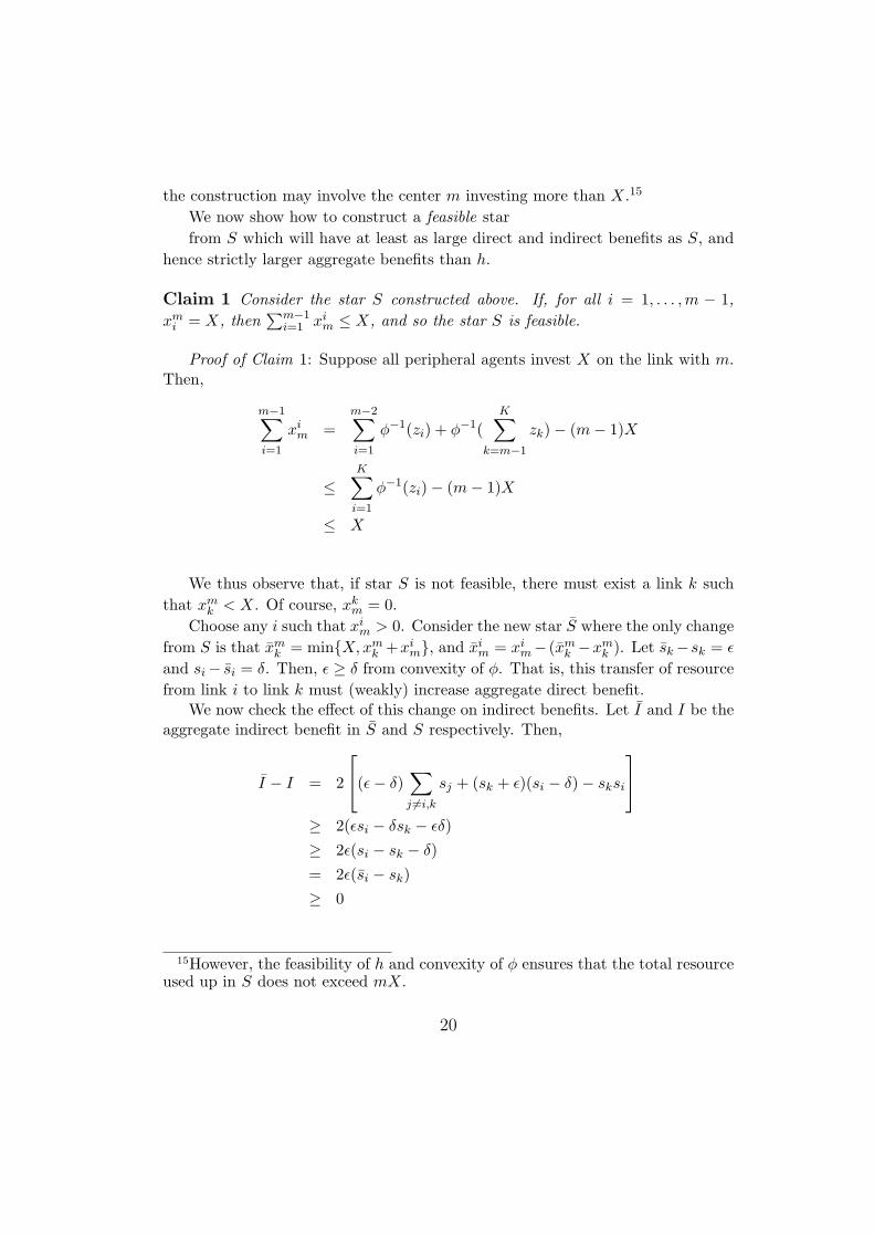
the construction may involve the center m investing more than X.15

We now show how to construct a feasible starfrom S which will have at least as large direct and indirect benefits as S, and

hence strictly larger aggregate benefits than h.

Claim 1 Consider the star S constructed above. If, for all i = 1, . . . ,m − 1,xm

i = X, then∑m−1

i=1 xim ≤ X, and so the star S is feasible.

Proof of Claim 1: Suppose all peripheral agents invest X on the link with m.Then,

m−1∑i=1

xim =

m−2∑i=1

φ−1(zi) + φ−1(K∑

k=m−1

zk)− (m− 1)X

≤K∑

i=1

φ−1(zi)− (m− 1)X

≤ X

We thus observe that, if star S is not feasible, there must exist a link k suchthat xm

k < X. Of course, xkm = 0.

Choose any i such that xim > 0. Consider the new star S where the only change

from S is that xmk = min{X, xm

k +xim}, and xi

m = xim− (xm

k −xmk ). Let sk−sk = ε

and si− si = δ. Then, ε ≥ δ from convexity of φ. That is, this transfer of resourcefrom link i to link k must (weakly) increase aggregate direct benefit.

We now check the effect of this change on indirect benefits. Let I and I be theaggregate indirect benefit in S and S respectively. Then,

I − I = 2

(ε− δ)∑j 6=i,k

sj + (sk + ε)(si − δ)− sksi

≥ 2(εsi − δsk − εδ)≥ 2ε(si − sk − δ)= 2ε(si − sk)≥ 0

15However, the feasibility of h and convexity of φ ensures that the total resourceused up in S does not exceed mX.

20

The last inequality holds because si = φ(X) + φ(xim) ≥ φ(X) ≥ sk.

So, aggregate benefit is at least as high in S as it is in S. If S is not feasible,then we can continue to transfer resources from the hub to some peripheral nodein the same way, until some star with aggregate benefit at least as high as S isfeasible.

Proof of Step 2: Consider two feasible stars S1 and S2 of sizes s1 and s2.Construct a new star S∗of size s1 + s2 centered around the hub of S,m2, with thefollowing investments:

xm2∗i = X for all i 6= m2

xi∗m2

= xim2

In terms of direct benefits, the only change between the new star S∗ and the starsS1 and S2 is that the hub of S1 now invests fully on its link with m2. Given theconvexity of φ, this change must have weakly increased aggregate direct benefits.Consider next the indirect benefits in the new star, I∗ and the sum of indirectbenefits in the two stars, I1 + I2. Indirect benefits inside the star S2 have notchanged, and peripheral nodes of S2 have gained access to new indirect connections.Agents in the star S1 have gained access to new indirect connections to agents instar S2. We focus attention on the difference in aggregate indirect benefits foragents inside the star S1. New indirect connections linking the hub of S1,m1 to allthe players in S1 have been created. At the same time, the strength of an indirectconnection between two peripheral nodes i and j of S1 has been decreased from(φ(X)+φ(xi

m1))(φ(X)+φ(xj

m1)) to φ(X)2. The difference in indirect benefits canthus be computed as:

∆I1 = 2(s1 − 1)φ(X)2 −∑

i,j∈S1\m1

φ(X)(φ(xim1

) + φ(xjm1

))−∑

i,j∈S1\m1

φ(xim1

)φ(xjm1

).

= 2(s1 − 1)φ(X)2 − 2(m− 2)φ(X)∑

i∈S1\m1

φ(xim1

)−∑

i,j∈S1\m1

φ(xim1

)φ(xjm1

).

By convexity of φ, ∑i∈S1\m1

φ(xm1i ) ≤ φ(X)

and ∑i,j∈S1\m1

φ(xim1

)φ(xjm1

) <∑

i∈S1\m1

φ(xm1i )2 ≤ φ(X)2

21

so that∆I1 > 0.

Hence, aggregate indirect benefits have increased after the merger of the two stars.As the same argument can be repeated with any pair of stars, we have completedstep 2 and the proof of the first statement of the Theorem.

Next, suppose that φ is linear. Let S∗ be the star with hub at n, where all arcshave strength X + X

n−1 . Let S be any other star with hub n where sin may not

be equal to sjn for i 6= j, but wheren−1∑i=1

(xni + xi

n) = nX. Of course, total direct

benefits are maximized at both S∗ and S. We now show that the sum of indirectbenefits in S∗ is greater than that in S.

Without loss of generality let s1n and s2n denote the weakest and strongest linksin S. Consider the effect of increasing investment on s1n by ε and simultaneouslydecreasing investment on s2n by ε.

The effect on the overall value can be computed as

∆V = 2[ε(s2n − s1n)− ε2]

Hence, for ε small enough, ∆V > 0 and so local changes in the direction ofequalization are profitable. But this implies that the symmetric star has highervalue than the asymmetric star. �

Several lemmas precede the proof of Theorem 2.

Lemma 1 Suppose φ is strictly convex, and g is a connected network which isNash stable. Then, all agents invest in a single link.

Proof. For any pair of connected agents (i, j), let W ji denote the equilibrium

marginal value to i of the connection with j – namely the value of the directconnection to j, and of all indirect connections to agents that i accesses throughj.

Suppose that agent i actually invests on two links to agents j and k. Theequilibrium values of the connections to j and k are given by

Wi = (φ(xji ) + φ(xi

j))Wji + (φ(xk

i ) + φ(xik))W

ki .

Suppose without loss of generality that W ji ≥ W k

i , and consider a deviation, whereagent i invests xj

i + xki on the link with agent j. This will result in a change in

utility∆Wi ≥ W j

i φ(xji + xk

i )−W ji φ(xj

i )−W ki φ(xk

i ) > 0,

22

concluding the proof of the Lemma.

Lemma 2 Suppose φ is linear, and g is strongly pairwise stable. If there is anagent i who invests in multiple links, then all of i’s neighbors invest fully in thelink to i.

Proof. For any triple of agents (i, j, k) where ij, jk ∈ g, let W j,ki denote the

equilibrium marginal value to i of the connection to k through j.Suppose that agent i invests on two links to agents j and k. There are two

cases to consider.Case 1: Both j and k invest on two or more links, so that xi

j < X and xik < X.

Assume that sij ≤ sik. We construct a joint reallocation of resources for playersi and j which makes both players strictly better off. Consider first a reallocation,where agent i shifts ε resources from the link to k to the link to j . Because φis linear and player i invests in both links, the marginal values of the connectionsto j and k must be equal, that is W j

i = W ki . Hence, by reallocating investment

to the link with j , agent i’s utility cannot decrease. Consider now the utility toagent j of the connection to i :

Wj = sij(1 + sikWi,kj +

∑m6=j,k

simW i,mj ).

Hence, the reallocation of investment will result in a utility change

∆Wj = ε(1 +∑

m6=j,k

silWi,mj + W i,k

j (sik − sij))− ε2W i,kj .

For ε close to zero, the change in utility is positive as sij ≤ sik.Next, consider an agent l such that xl

j > 0 and consider a reallocation whereagent j shifts δ resources from the link to l to the link to i. Because xi

j may beequal to zero, this reallocation may result in a utility loss for agent j. However,this utility loss must be continuous in δ and hence, for any ε, one can find δ(ε),such that the total effect of the reallocation of resources (δ, ε) on the utility of j isstrictly positive. Now consider agent i. Since agent i could have chosen to connectdirectly to agent l, the equilibrium marginal value of i’s connection to j must beat least as large as the marginal value of a possible direct connection to l. So,

W ji = 1 + sjlW

j,li +

∑m6=i,l

sjmW j,mi ≥ W j,l

i . (4)

23

Now the effect of the reallocation of resources δ on the utility of agent i is givenby:

∆Wi = δ(1 +∑

m6=i,l

sjmW j,mi + W j,l

i (sjl − sij))− δ2W j,li .

Using equation 4,∆Wi ≥ δ(1− sij)W

j,li − δ2W j,l

i ,

which is strictly positive for δ close to zero. Hence, we have constructed a jointreallocation of resources which makes both players i and j strictly better off.

Case 2: Suppose xij = X, but xi

k < X.From the proof above, it is clear that if sij ≥ sik, then individuals i and k can

jointly plan a profitable deviation. So, assume that sij < sik. Since xij = X, this

means that X > xik > 0. Let xl

k > 0 for some l. Since i invests on k, W ki ≥ W l

i .Similarly, since k invests on i, W i

k ≥ W jk . Suppose k transfers some resource from

the link to l to the link to i. Then, i’s total utility strictly increases since he getsthe additional direct benefit, and there cannot be any loss in indirect benefit sinceW k

i ≥ W li . Moreover, k is indifferent since W i

k = W ik. For an exactly analogous

reason, a transfer of resource by i from the link to j to the link to k makes k betteroff and leaves i indifferent. So, i and k have a profitable joint deviation.

Lemma 3 Let g be a connected network which is not a tree. Then,(i) If φ is strictly convex, then g is not Nash stable.(ii) If φ is linear, then g is not strongly pairwise stable.

Proof. Let g contain a cycle {(12), (23), . . . , (r − 1, r), (r1)}. Denote R ={1, 2, . . . , r}.

(i) Since φ is strictly convex, Lemma 1 implies that all agents invest only onone link. For each i ∈ R, let Li denote the set of nodes contained in N \R whichcan be accessed through node i. Note that each pair Li, Lj must be disjoint sets -since agents invest in only one link, there can be at most one cycle.

Let Vi be the total benefit that i gets from nodes in Li. We first show thatVi ≡ V for all i ∈ R.

Suppose not, so that Vi 6= Vj for some i, j ∈ R. Then, there must be a pair ofadjacent nodes i, i + 1 such that Vi+1 > Vi. Then, i− 1 is better off connecting toi + 1 rather than to i. Hence, Vi ≡ V for all i ∈ R.

So, i gets a benefit of φ(X)k from node i + k in R and φ(X)kV from nodes inLi+k. Let B = 1 + V . Then, if r is odd, agent i initially obtains

Ui = 2B

(r−1)/2∑k=1

φ(X)k

24

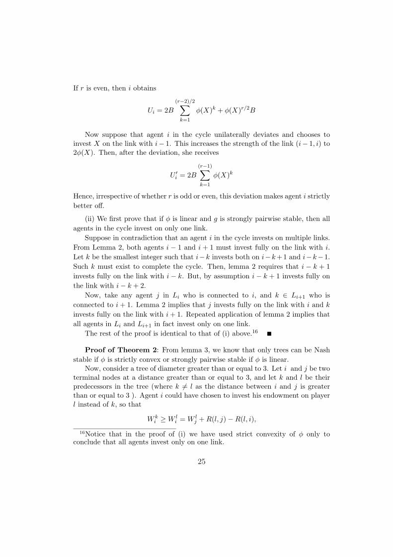
If r is even, then i obtains

Ui = 2B

(r−2)/2∑k=1

φ(X)k + φ(X)r/2B

Now suppose that agent i in the cycle unilaterally deviates and chooses toinvest X on the link with i− 1. This increases the strength of the link (i− 1, i) to2φ(X). Then, after the deviation, she receives

U ′i = 2B

(r−1)∑k=1

φ(X)k

Hence, irrespective of whether r is odd or even, this deviation makes agent i strictlybetter off.

(ii) We first prove that if φ is linear and g is strongly pairwise stable, then allagents in the cycle invest on only one link.

Suppose in contradiction that an agent i in the cycle invests on multiple links.From Lemma 2, both agents i − 1 and i + 1 must invest fully on the link with i.Let k be the smallest integer such that i−k invests both on i−k +1 and i−k−1.Such k must exist to complete the cycle. Then, lemma 2 requires that i − k + 1invests fully on the link with i− k. But, by assumption i− k + 1 invests fully onthe link with i− k + 2.

Now, take any agent j in Li who is connected to i, and k ∈ Li+1 who isconnected to i + 1. Lemma 2 implies that j invests fully on the link with i and k

invests fully on the link with i + 1. Repeated application of lemma 2 implies thatall agents in Li and Li+1 in fact invest only on one link.

The rest of the proof is identical to that of (i) above.16

Proof of Theorem 2: From lemma 3, we know that only trees can be Nashstable if φ is strictly convex or strongly pairwise stable if φ is linear.

Now, consider a tree of diameter greater than or equal to 3. Let i and j be twoterminal nodes at a distance greater than or equal to 3, and let k and l be theirpredecessors in the tree (where k 6= l as the distance between i and j is greaterthan or equal to 3 ). Agent i could have chosen to invest his endowment on playerl instead of k, so that

W ki ≥ W l

i = W lj + R(l, j)−R(l, i),

16Notice that in the proof of (i) we have used strict convexity of φ only toconclude that all agents invest only on one link.

25

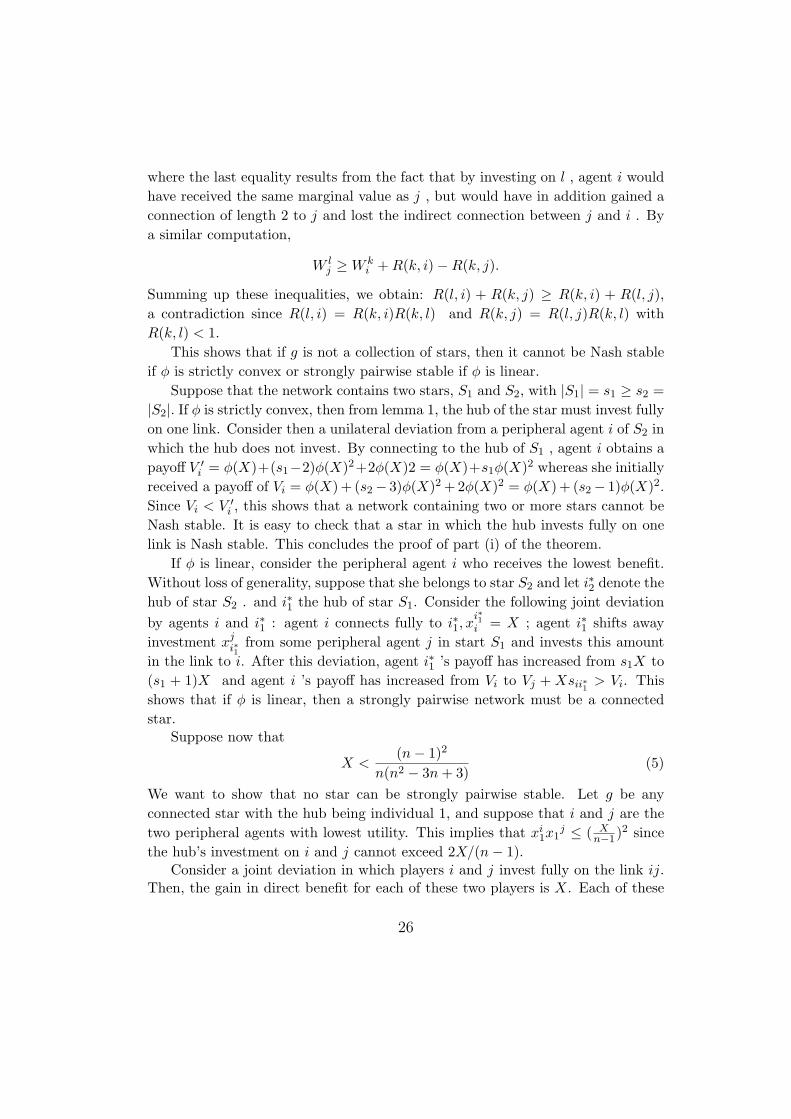
where the last equality results from the fact that by investing on l , agent i wouldhave received the same marginal value as j , but would have in addition gained aconnection of length 2 to j and lost the indirect connection between j and i . Bya similar computation,

W lj ≥ W k

i + R(k, i)−R(k, j).

Summing up these inequalities, we obtain: R(l, i) + R(k, j) ≥ R(k, i) + R(l, j),a contradiction since R(l, i) = R(k, i)R(k, l) and R(k, j) = R(l, j)R(k, l) withR(k, l) < 1.

This shows that if g is not a collection of stars, then it cannot be Nash stableif φ is strictly convex or strongly pairwise stable if φ is linear.

Suppose that the network contains two stars, S1 and S2, with |S1| = s1 ≥ s2 =|S2|. If φ is strictly convex, then from lemma 1, the hub of the star must invest fullyon one link. Consider then a unilateral deviation from a peripheral agent i of S2 inwhich the hub does not invest. By connecting to the hub of S1 , agent i obtains apayoff V ′

i = φ(X)+(s1−2)φ(X)2+2φ(X)2 = φ(X)+s1φ(X)2 whereas she initiallyreceived a payoff of Vi = φ(X) + (s2 − 3)φ(X)2 + 2φ(X)2 = φ(X) + (s2 − 1)φ(X)2.Since Vi < V ′

i , this shows that a network containing two or more stars cannot beNash stable. It is easy to check that a star in which the hub invests fully on onelink is Nash stable. This concludes the proof of part (i) of the theorem.

If φ is linear, consider the peripheral agent i who receives the lowest benefit.Without loss of generality, suppose that she belongs to star S2 and let i∗2 denote thehub of star S2 . and i∗1 the hub of star S1. Consider the following joint deviationby agents i and i∗1 : agent i connects fully to i∗1, x

i∗1i = X ; agent i∗1 shifts away

investment xji∗1

from some peripheral agent j in start S1 and invests this amountin the link to i. After this deviation, agent i∗1 ’s payoff has increased from s1X to(s1 + 1)X and agent i ’s payoff has increased from Vi to Vj + Xsii∗1

> Vi. Thisshows that if φ is linear, then a strongly pairwise network must be a connectedstar.

Suppose now that

X <(n− 1)2

n(n2 − 3n + 3)(5)

We want to show that no star can be strongly pairwise stable. Let g be anyconnected star with the hub being individual 1, and suppose that i and j are thetwo peripheral agents with lowest utility. This implies that xi

1x1j ≤ ( X

n−1)2 sincethe hub’s investment on i and j cannot exceed 2X/(n− 1).

Consider a joint deviation in which players i and j invest fully on the link ij.Then, the gain in direct benefit for each of these two players is X. Each of these

26

players loses an indirect benefit of X(X + xk1) from each player k 6= 1, i, j and the

indirect benefit of (X +xi1)(X +xj

1). So, the total loss in indirect benefit to playerl, l = i, j is

L = X∑

k 6=1,i,j

(X + xk1) + (X + xi

1)(X + xj1)

= (n− 1)2X2 + xi1x

j1

≤ (n− 1)2X2 +X2

(n− 1)2

< X

where the last inequality follows from equation 5. This shows that if the inequalityin equation 5 holds, then the set of strongly pairwise networks is empty.

Conversely, consider the connected star in which the hub invests equally oneach link, and suppose that X ≥ (n−1)2

n(n2−3n+3). As the hub of the star gets the

maximal payoff, nX, she never has any incentive to deviate. No peripheral agenthas any unilateral profitable deviation. Now, consider a joint deviation by a pairof peripheral agents i, j. The only possible such deviation is for player i to shiftsome resource from her investment on the link with the hub to a link with player j,and for player j to reciprocate. Given the linearity of φ, if this deviation is jointlyprofitable for transfers (δi, δj), then it is profitable when i and j invest fully ontheir own link. Then, the gain in direct benefit is X. The loss in indirect benefitis exactly (n − 1)2X2 + X2

(n−1)2≤ X. Hence, the connected star in which the hub

invests an equal amount on each link is strongly pairwise stable. This completesthe proof of the theorem. �

Proof of Theorem 3:(i) The proof follows the same lines as the proof of Theorem 1.

Step 1: Observe first that we can restrict attention to trees. If a networkcontains a cycle, then consider the weakest link on the cycle, and reallocate theinvestments over the other links. Since the weakest link in the cycle was never usedon any path (or agents were indifferent between using it or an alternative path), thisreallocation must weakly increase the aggregate benefits in the network. Considernow any tree h on m nodes, with link strengths {z1, . . . , zm−1}, and the star Scorresponding to h as in the proof of Theorem 1. Denote the link strengths in Sas {s1, . . . , sm−1}. Direct benefits are exactly identical in S and in h. The sum ofindirect benefits in the star S is easily calculated.

I = 2m−2∑i=1

(m− i− 1)sm−i

27

To check this, note that the link sm−1 is the minimum in all comparisons, and so thesum of indirect benefits obtained between m− 1 and other nodes is 2(m− 2)sm−1.Similarly, sm−2 is the minimum in (m− 3) comparisons and so on.

Now, consider indirect benefits in h. Note that the arc zm−1 must also beinvolved in at least (m − 2) comparisons in the graph h (the minimum beingattained if zm−1 connects some terminal node). Similarly, for any t, the t arcswith the lowest values, {zm−t, ..., zm−1} must be the minimum in at least (m −2) + (m− 3) + ... + (m− t− 1) connections (the minimum being attained if theyboth connect to some terminal node). This establishes that the sum of direct andindirect benefits is at least as high in S as in h.

Step 2: We now show that if the graph contains two stars S1 and S2, it isdominated by the graph where the two stars are merged into a single star, as inthe proof of Theorem 1. By merging the two stars into a single star with hub m2,direct benefits have increased. Furthermore, indirect benefits for players in star S2

have strictly increased. For a peripheral agent i in star S1, indirect benefits wereequal to

Ii =∑

j∈S1\m1

φ(X) + min{φ(xim1

), φ(xjm1

)}

= (m1 − 1)φ(X) +∑

j∈S1\m1

min{φ(xim1

), φ(xjm1

)}.

In the new star, indirect benefits are given by:

I∗i = (m1 + m2 − 1)φ(X).

As m2 ≥ 1 and φ(X) ≥∑

j∈S1\m1min{φ(xi

m1), φ(xj

m1)}I∗i ≥ Ii and indirect bene-fits cannot have decreased.

This concludes the proof of part (i).

(ii) Next suppose that φ is linear, and that the hub invests different amountson its links with peripheral nodes. Let i be a node for which xi

n is maximal, and j anode for which xj

n is minimal. Consider a reallocation of investments, xin = xi

n−ε,

xjn = xj

n + ε. This reallocation does not affect direct benefits. For ε small enough,it only reduces indirect benefits between i and other players who are connected tothe hub by links of maximal strength by ε. Indirect benefits between player j andall these players have been increased by ε, and indirect benefits between players i

and j have strictly increased. Hence, this reallocation of investments has strictlyincreased the value of the graph, showing that the hub must put equal weight onall links with peripheral agents.

28

Now, in the symmetric star, each link has strength (X + Xn−1). Since there are

n − 1 links, each agent gets a benefit of nX. Since this equals the total resourceavailable, the symmetric star must be strongly pairwise stable.

(iii) To show that, if φ is strictly convex, the star where the hub invests on asingle link is strongly pairwise stable, notice that the hub and the peripheral agentin which he invests obtain the maximal benefit of nφ(X) and have no incentive tomove.

Other peripheral agents have a benefit of (n−1)φ(X). If two peripheral agentsmove, they have no incentive to reallocate their links in such a way that they forma cycle. Hence, either they reallocate all their investments on their link and theyobtain 2φ(X) which is smaller than their initial payoff. Or one of them reallocateshis investment from the hub to the peripheral agent, resulting in the same payoffof (n− 1)φ(X) as before. Hence, there does not exist any profitable deviation. �

Proof of Theorem 4: (i) Suppose g is efficient and has a component with three ormore nodes, where two nodes have degree one. Denote these nodes by i and j andtheir immediate predecessors by k and l respectively. Because the component isconnected, the degrees of k and l are necessarily greater than one. But this impliesthat xi

k < X and xjl < X . Furthermore because

∑m∈N\{i}

xmk ≤ X, xm

k ≤ X − xik

for all node m 6= i to which k is connected. Now, this implies that the valueof the indirect connection between i and j in the graph is strictly smaller thanmin{X − xi

k, X − xjl }. Furthermore, in an efficient graph, xk

i = xik and xl

j = xjl

so that individual i can invest X − xik in the direct link with j and individual j

can invest X − xjl in the link with i . But, because the value of the indirect link

is smaller than min{X − xik, X − xj

l } , the investment in the direct link strictlyincreases the value of the graph, yielding a contradiction. This completes the proofof part (i).

(ii) To show that the symmetric circle is efficient for low values of n, considerthe different values of n in turn. For n = 3 , the circle is the only connected graphwhich is not a tree. Now, notice that direct benefits are equal to nX and henceare maximal in the circle. For n = 4, 5 , we show that the circle also maximizesthe value of indirect benefits. Notice first that the value of an indirect connectionis always bounded above by (X/2)2 as the middle player must allocate X over atleast two links. For n = 4 and n = 5 all indirect connections in the circle areof length 2 and have value (X/2)2 . Hence, the circle achieves the highest sumof indirect links and is efficient. It is easy to check that any other allocation ofinvestments results in a lower value of indirect links, so the circle with links of

29

equal strength is uniquely efficient.Suppose now that n = 6, 7. The indirect benefit for any node in the circle is

I =X2

2+

X3

4

Consider any other graph g. If this graph is to “dominate” the cycle, then atleast one node (say i∗ ) has to derive an indirect benefit exceeding I . For each k

, check that the circle maximizes indirect benefits from nodes at a distance of k.So, if i is to derive a larger indirect benefit in g, it must have more than two nodesat a distance of 2.17

It is tedious to show that the maximum indirect benefit that i∗ can deriveoccurs when i∗ has two neighbors, j1, j2 , with each neighbor of i∗ having threeneighbors including i∗ itself. Moreover, the optimum pattern of allocation fromthe point of view of i∗ is

xj1i = xj2

i = xij2 = xi

j2 =12

This yields i∗ a total indirect benefit of X2

2 < I .This completes the proof of part(ii).

(iii) Finally, we show that the symmetric circle is strongly pairwise stable. Inthe symmetric cycle, each i gets a direct benefit of X. No pattern of investmentcan result in higher direct benefits. So, we check whether a deviation by i and j

can improve their indirect benefits.Suppose i and j are neighbors in the cycle. Consider the effect on i of increasing

investment to X2 +y by both i and j on the link ij, and decreasing their investments

on their other neighbors by y. The change in indirect benefit for i from j’s otherneighbor is (X

2 + y)(X2 − y) − (X

2 )2 < 0. A similar calculation shows that i alsoloses from nodes which are further away.

Suppose i and j are not neighbors in the cycle. Let i and j mutually investy each on the link ij and simultaneously decrease investment on their previousneighbors by y

2 . It is easy to check that this is the best possible deviation.Clearly, this can only increase indirect benefit for i if there is some k such that

the distance between i and k is now lower. This means that i accesses k throughj. Let k be a neighbor of j. Then, the indirect benefit for i from k is

I = y(X − y

2) =

Xy

2− y2

217Since n ≤ 7, the maximum distance between any two nodes in the circle is 3.

30

Now, i has reduced the strength of links with each of its previous neighbors byy2 . Also, since k is not at a distance of 2 from i in the cycle, there must be somenode m, distinct from k which is at a distance of 2 from i. The loss in indirectbenefit for i from m is

I ′ = (X − y

2)X

2− X2

4=

Xy

2

Hence, the indirect benefit for i from k is lower than the loss in indirect benefitfrom m.

Repeating this argument, it can be shown that i’s total indirect benefit willactually go down as a result of the deviation. �

31