Communication and localization in the context of aerial

robotics (UAVs)

A Degree Thesis

Submitted to the Faculty of the

Escola Tècnica d'Enginyeria de Telecomunicació de

Barcelona

Universitat Politècnica de Catalunya

by

Adrià Sáez Mediavilla

In partial fulfilment

of the requirements for the degree in

Telecommunication System ENGINEERING

Advisor: Andrea Tonello

Klagenfurt, June 2018

1

Abstract

This project consists on the communication and localization of a drone (Mobile Station

MS). In order to do so, several simulations have been done with Matlab to send and

receive bits, as well as for simulating the ToA (Time of Arrival). Afterwards, USRP (some

hardware plaques) have been used to implement the code made on MatLab and

LabView; these USRP have been programmed with a software called LabView and,

finally, it has been possible to send and receive correctly the bits and calculate the ToA.

Lastly, this document explains the simulations, implementations, the state of art on

modern technology, the costs of this project and the conclusions.

2

Resum

Aquest projecte consisteix en la comunicació i localització d’un dron (MS). Per tant, s’han

fet varies simulacions amb MatLab per enviar uns bits i rebre els mateixos bits, i també

per simular el ToA (Time of Arrival). Seguidament, s’han utilitzat unes USRP (unes

plaques software), per implementar el codi fet en MatLab. Aquestes USRP s’han

programat amb un programa que es diu LabView i al final de tot, s’ha aconseguit enviar i

rebre correctament uns bit i també calcular el ToA.

Finalment, en aquest document s’explicaran les simulacions, les implementacions, l’estat

de l’art de la tecnologia actual, el cost que ha tingut aquest projecte i les conclusions.

3

Resumen

Este proyecto consiste en la comunicación y localización de un dron (MS). Por lo tanto,

se han hecho varias simulaciones con MatLab para enviar unos bits y recibir los mismos

bits, y también para simular el ToA (Time of Arrival). Seguidamente, se han usado unas

USRP (unas placas hardware), para implementar el código hecho en MatLab. Estas

USRP se han programado con un programa llamado LabView y al final del todo se ha

conseguido enviar y recibir correctamente unos bits y también calcular el ToA.

Finalmente, en este documento se explican las simulaciones, las implementaciones, el

estado del arte de la tecnología actual, el costo que ha tenido este proyecto y las

conclusiones.

4

Dedication

I would like to dedicate this project, first of all, to every teacher of my university that I had

during these years of my degree, since without them, I wouldn’t learn everything that I

learnt and I wouldn’t be able to do this project. Also, I would like to dedicate to them this

project because they are who have motivated me always to go ahead with the degree

and not to leave it.

On the other hand, also I would like to dedicate this proposal to every one of my mates

that I have had at the Klagenfurt university, that have been with me every day, helping

and advising me in each moment.

Also, I would like to dedicate this draft to my family, my girlfriend and to my friends, that

always have been helping me and supporting me in each of my decisions, and also, the

influenced me in the option to could come here to do my final degree thesis, in a foreign

country.

Last, but not least, I would like to dedicate this project to my 2 tutors that I have had

during the course of this proposal: Ramon Ferrús y Andrea Tonello, because they have

been who have helped me to go ahead with the project and who have advised me in

each moment.

5

Acknowledgements

During my stay at the University of Klagenfurt, almost all my acknowledgement went to

(the internet) and all the members of the laboratory, because I have been working with a

small group PHD telecommunication and electronic students from around the world,

leaded by my tutor, Andrea Tonello.

I shall also thank the official manufacturers of the hardware that I have used during the

project, Ettus company (https://www.ettus.com/), since they have a wide web page where

you can find any information related to its hardware. Moreover, I have send and received

a lot of emails from the Ettus and from the MathWorks support team when I needed

support for using the code for the hardware.

To finish with, I must thank my tutor Andrea Tonello, who gave a lecture on advanced

communications, which I assisted and I could learn a lot of useful skills for my project.

6

Revision history and approval record

Revision Date Purpose

0 02/06/2018 Document creation

1 03/06/2018 Document revision

2 06/06/2018 Document revision

3 07/06/2018 Document revision

4 08/06/2018 Document revision

5 10/06/2018 Document revision

6 12/06/2018 Document revision

7 13/06/2018 Document revision

8 16/06/2018 Document revision

9 17/06/2018 Document revision

10 18/06/2018 Document revision

11 20/06/2018 Document revision

12 23/06/2018 Final Revision

DOCUMENT DISTRIBUTION LIST

Name e-mail

Adrià Sáez adriasaez@hotmail.com

Tonello, Andrea M. andrea.tonello@aau.at

Ramon Ferrús ferrus@tsc.upc.edu

Written by: Reviewed and approved by:

Date 01/06/2018 Date 25/06/2018

Name Adrià Sáez Name Andrea Tonello

Position Project author Position Project Supervisor

7

Table of contents

Communication and localization in the context of aerial robotics (UAVs) ........................... 0

Abstract................................................................................................................................. 1

Resum................................................................................................................................... 2

Resumen .............................................................................................................................. 3

Acknowledgements .............................................................................................................. 5

Revision history and approval record................................................................................... 6

Table of contents .................................................................................................................. 7

List of Figures ....................................................................................................................... 9

List of Tables: ..................................................................................................................... 11

1. Introduction.................................................................................................................. 12

1.1. Statement of purpose .......................................................................................... 12

1.2. Requirements and specifications. ....................................................................... 13

1.3. Methods and procedures ..................................................................................... 13

1.4. Work plan ............................................................................................................. 13

1.5. Description of the deviations ............................................................................... 15

2. State of the art of the technology used or applied in this thesis:................................ 16

2.1. Overview of he main radiolocation methods ....................................................... 16

2.1.1. Basic methods used in positioning systems ................................................ 17

2.1.1.1. TOA Estimation .......................................................................................... 17

2.1.1.2. Time - Difference - of - Arrival (TDOA) Estimation .................................... 18

2.1.1.3. DOA Estimation .......................................................................................... 19

2.1.1.4. RSSI ........................................................................................................... 20

2.1.2. Fundamental differences.............................................................................. 20

2.2. Actual SDR companies/products......................................................................... 21

2.2.1. Ettus Research, and NI Company ............................................................... 21

2.3. USRP used in the lab .......................................................................................... 22

2.3.1. USRP B205mini............................................................................................ 22

2.3.2. USRP B210 .................................................................................................. 23

2.3.3. USRP X310 .................................................................................................. 24

2.3.4. NI USRP 2954R ........................................................................................... 25

3. Methodology / project development: ........................................................................... 26

3.1. Simulations .......................................................................................................... 26

3.1.1. Communication Transmitter-Receiver ......................................................... 26

8

3.1.1.1. Channel ...................................................................................................... 27

3.1.1.2. Channel estimation .................................................................................... 28

3.1.1.3. Equalizer..................................................................................................... 28

3.1.1.4. Receiver and transmitter filters .................................................................. 29

3.1.2. Time of Arrival simulation (ToA) ................................................................... 30

3.1.3. Positioning simulation................................................................................... 31

3.2. Implementation .................................................................................................... 31

3.2.1. ToA ............................................................................................................... 31

3.2.1.1. Base station................................................................................................ 32

3.2.1.2. Mobile station ............................................................................................. 34

4. Results......................................................................................................................... 36

4.1. Simulation Results ............................................................................................... 36

4.1.1. Transmitter – Receiver Communication simulation ..................................... 36

4.1.2. ToA Simulation ............................................................................................. 38

4.1.3. Position Simulation ....................................................................................... 39

4.2. Implementation results ........................................................................................ 40

4.2.1. ToA results.................................................................................................... 40

4.2.1.1. Base station................................................................................................ 41

4.2.1.2. Mobile station ............................................................................................. 42

5. Budget ......................................................................................................................... 43

6. Conclusions and future development: ........................................................................ 44

Bibliography: ....................................................................................................................... 45

Glossary.............................................................................................................................. 46

9

List of Figures

- Figure 1: Gantt diagram …………………………………………………………………………………………………...… pag 15

- Figure 2: Futuristic applications for positioning systems ………………………………………………….. pag 16

- Figure 3: Positioning system classification ………………………………………………………………………… pag 16

- Figure 4: Operation of TOA and RSSI ………………………………………………………………………………..… pag 17

- Figure 5: Operation of TDOA ……………………………………………………………………………………………… pag 18

- Figure 6: Comparison of TOA and TDOA calculations ………………………………………………………… pag 19

- Figure 7: Operation of DOA ………………………………………………………………………………………………… pag 19

- Figure 8: USRP B200mini …………………………………………………………………………………………………… pag 22

- Figure 9: USRP B205mini architecture …………………………………………………………………………….… pag 23

- Figure 10: USRP B210 ………………………………………………………………………………………………………… pag 23

- Figure 11: USRP X310 ………………………………………………………………………………………………………… pag 24

- Figure 12: USRP 2954R …………………………………………………………………………………………………….… pag 25

- Figure 13: Transmitter …………………………………………………………………………………………………….… pag 25

- Figure 14: Channel …………………………………………………………………………………………………………….. pag 26

- Figure 15: Receiver ………………………………………………………………………………………………………….… pag 27

- Figure 16: Channel design ………………………………………………………………………………………………..… pag 27

- Figure 17: Multipath/Rayleig channel ……………………………………………………………………………….. pag 28

- Figure 18: Equalizer …………………………………………………………………………………………………………… pag 29

- Figure 19: Root Raised cosine filter ………………………………………...…………………………………………. pag 29

- Figure 20: CrossCorrelation …………………………………………………………………………………………….…. Pag30

- Figure 21: Model diagram ………………………………………………………………………………………………..… pag 31

- Figure 22: BS Transmitter ………………………………………………………………………………………………..… pag 31

- Figure 23: BS Receiver 1 …………………………………………………………………………………………………..… pag 32

- Figure 24: BS Receiver 2 …………………………………………………………………………………………………….. pag 32

- Figure 25: ToA with time ………………………………………………………………………………………………….… pag 33

- Figure 26: ToA with correlation ……………………………………………………………………………………….… pag 33

- Figure 27: MS receiver 1 …………………………………………………………………………………………………..… pag 33

- Figure 28: MS receiver 2 …………………………………………………………………………………………………..… pag 34

- Figure 29: MS transmitter ………………………………………………………………………………………………..… pag 34

- Figure 30: Our BPSK signal after the Tx filter and before the channel ……………………………..… pag 35

- Figure 31: Our Signal through the Channel ………………………………………………………………………… pag 35

- Figure 32: Signal after the equalizer ………………………………………………………………………………….. pag 36

10

- Figure 33: Channel & Channel estimation ………………………………………………………………………..… pag 36

- Figure 34: Modulated Signal vs. received modulated signal …………………………………………….… pag 37

- Figure 35: ToA simulation results ……………………………………………………………………………………… pag 38

- Figure 36: Transmitted and received signal ………………………………………………………………………. pag 38

- Figure 37: Followed path by the MS …………………………………………………………………………………… pag 39

- Figure 38: BS transmitter Panel ……………………………………………………………………………………….… pag 40

- Figure 39: BS receiver panel ………………………………………………………………………………………………. pag 40

- Figure 40: MS receiver panel ……………………………………………………………………………………………… pag 41

- Figure 41: MS transmitter panel ………………………………………………………………………………………… pag 41

11

List of Tables:

Table 1: Comparison of basic Methods …………………………………………………………………………………………..… pag 20

12

1. Introduction

Wireless location has received considerable attention over the past few years. The basic

function of a location system is to gather information about the position of a mobile station

(MS) operating in a geographical area and process that information to form a location

estimate. A popular approach, known as radiolocation, measures parameters of radio

signals that travel between an MS and a set of fixed transceivers, which are subsequently

used to derive the location estimate. [1]

Radiolocation is the process of finding the location of something through the use of radio

waves. It generally refers to passive uses, particularly radar—as well as detecting buried

cables, water mains, and other public utilities. It is similar to radio navigation, but

radiolocation usually refers to passively finding a distant object rather than actively one's

own position. Both are types of radio determination. Radiolocation is also used in real-

time locating systems (RTLS) for tracking valuable assets.

An object can be located by measuring the characteristics of received radio waves. The

radio waves may be transmitted by the object to be located, or they may

be backscattered waves (as in radar or passive RFID, Radio Frequency Identification).

Many existing wireless location systems, such as the Global Positioning System (GPS)

and Loran C, make use of radiolocation techniques. With these technologies, the MS

formulates its own position, which can be relayed to a central site. Some approaches

employ a cellular network as the transport mechanism for relaying the location estimate

[2].

Radiolocation systems can be implemented in one of two ways. With the first approach,

the MS uses signals transmitted by the BSs to calculate its own position, as in GPS. With

the second approach, the BSs measure the signals transmitted by the MS and relay them

to a central site for processing. The second approach has the advantage of not requiring

any modifications or specialized equipment in the MS handset, thus accommodating the

large pool of handsets already in use in existing cellular networks

1.1. Statement of purpose

The purpose of this project is to understand real hardware and radio propagation aspects,

acquire competence in signal acquisition and real time signal processing, as well as to

learn about the specific UAV (Unmanned Aerial Vehicle) application. This application

consists on locating the UAV with one transmitter, which will be a base station

responsible for estimating the location and one receiver located inside of the UAV. To

achieve this, there will be used SDR (Software-Defined Radios), and more specifically

USRP that are some SDR from the Ettus company.

Software-defined radio (SDR) is a radio communication system where components that

have been traditionally implemented in hardware are instead implemented by means of

software on a personal computer or embedded system.

13

1.2. Requirements and specifications.

Project requirements:

- Ability to using simulation tools (MatLab, Simulink, LabView)

- Handling of handle with hardware tools

- The knowledge of the student about telecommunications.

Project specifications:

- Understand real hardware and radio propagation aspects

- Acquire competence in signal acquisition

- Acquire competence in real time signal processing

- Learn about the specific UAV applications

1.3. Methods and procedures

For the realization of this project, hardware from the Ettus Company has been used,

which will be explained on the section "State of Art" with all its characteristics.

Moreover, a code has been written from scratch for the simulation and its further

implementation on the hardware.

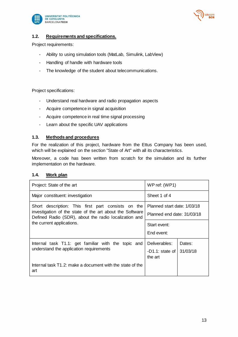
1.4. Work plan

Project: State of the art WP ref: (WP1)

Major constituent: investigation Sheet 1 of 4

Short description: This first part consists on the

investigation of the state of the art about the Software

Defined Radio (SDR), about the radio localization and

the current applications.

Planned start date: 1/03/18

Planned end date: 31/03/18

Start event:

End event:

Internal task T1.1: get familiar with the topic and

understand the application requirements

Internal task T1.2: make a document with the state of the

art

Deliverables:

-D1.1: state of

the art

Dates:

31/03/18

14

Project: Algorithms & Simulations WP ref: (WP2)

Major constituent: investigation & simulation (software) Sheet 2 of 4

Short description: This part will consist on the study of the

main algorithms for radio localization using antenna arrays.

Furthermore, it will be important to get familiar with

simulation tools for the analysis of the algorithms, e.g.,

Matlab, and for the implementation in the experimental

platform based on software defined radios, e.g., Labview or

GNU Radio

Planned start date: 20/03/18

Planned end date: 31/05/18

Start event:

End event:

Internal task T2.1: study the main algorithms for radio

localization using antenna arrays.

Internal task T2.2: Get familiar with the simulation tools.

Deliverables:

-D2.1:

algorithms of

radio

localization

Dates:

31/05/18

Project: Implementation WP ref: (WP3)

Major constituent: hardware prototype, simulation, SW Sheet 3 of 4

Short description: this part will carry out experimental

activities by implementing an algorithm, simulating and

analysing its performance. It will be also possible to implement

it on the hardware platform using Labview

Planned start date:1/04/18

Planned end date: 29/06/18

Start event:

End event:

Internal task T3.1: implement an algorithm

Internal task T3.2: simulate and analyse the algorithm

performance

Deliverables:

-D3.1:

prototype

Dates:

29/06/18

Project: Documentation WP ref: (WP4)

Major constituent: documentation Sheet 4 of 4

Short description: this part consists on the management of the

entire project, in other words, to write some reports and do

Planned start date:1/03/18

Planned end date: 29/06/18

15

presentations (one in the middle and a final report), and to be

aware of the meetings with the professor, to manage the

project time. In addition, everything must be documented and

has to be disseminated.

Start event:

End event:

Internal task T4.1: manage all the project

Internal task T4.2: dissemination

Deliverables:

Each meeting

is a

deliverable

-D4.1:

midterm

report

-D4.2: final

report

Dates:

30/04/18

28/06/18

Figure 1: Gantt diagram

1.5. Description of the deviations

The final goal of this project was to locate the exact position of a mobile station (a drone)

with three base-stations (three USRP), to make the signal indictment on real time and to

display on a map the position and the track followed by the drone on real time.

The final test consisted on the communication of the two USRPs by the same method on

the simulation and on the application of a Time Of Arrival (ToA) algorithm to calculate, on

real time, the distance of the two USRP by moving them and seeing how the distance

changes.

01-març 26-març 20-abr. 15-maig 09-juny 04-jul. 29-jul.

WP1

WP2

WP3

WP4

16

2. State of the art of the technology used or applied in this

thesis:

2.1. Overview of he main radiolocation methods

Recent years have seen rapidly increasing demand for services and systems that depend upon accurate positioning of people and objects. This has led to the development and evolution of numerous positioning systems.

Figure 2: Futuristic applications for positioning systems

Figure 3: Positioning system classification

17

As shown in Figure 3, positioning systems can be classified into two categories:

1. Global Positioning

2. Local Positioning

Global positioning systems (GPSs) allow each mobile to find its own position on the globe. A local positioning system (LPS) is a relative positioning system and can be classified into self - and remote positioning. Self - positioning systems allow each person or object to find its own position with respect to a static point at any given time and location. An example of these systems is the inertial navigation system (INS). Remote positioning systems allow each node to find the relative position of other nodes located in its coverage area. Here, nodes can be static or dynamic. Remote positioning systems themselves are divided into

1. Active target remote positioning and

2. Passive target remote positioning.

In the first case, the target is active and cooperates in the process of positioning, while in the second, the target is passive and no cooperative.

2.1.1. Basic methods used in positioning systems

2.1.1.1. TOA Estimation

TOA estimation allows the measurement of distance, thus enabling localization. Here, multiple base nodes collaborate to localize a target node via triangulation [3]. It is assumed that the positions of all base nodes are known. If these nodes are dynamic, a positioning technique such as GPS is used to allow base nodes to locate their positions (GPS – TOA positioning). In some circumstances, multiple base nodes may cooperate to find their own position before any attempt to localize a target node [4]. Assuming known positions of base nodes and a coplanar scenario, three base nodes and three measurements of distances (TOA) are required to localize a target node (see Fig. 4). In a non - coplanar case, four base nodes are required. Using the measurement of distance, the position of a target node is localized within a sphere of radius Ri with the receiver i at the centre of the sphere (where Ri is directly proportional to the TOA as shown in Figure 4). The localization of the target node can be carried out either by base nodes using a master station or by the target node itself.

Figure 4: Operation of TOA and RSSI

18

Although TOA seems to be a robust technique, it has a few drawbacks [5]:

1. It requires all nodes (base nodes and target nodes) to precisely synchronize: A small timing error may lead to a large error in the calculation of the distance Ri.

2. The transmitted signal must be labelled with a time stamp in order to allow the base node to determine the time at which the signal was initiated at the target node. This additional time stamp increases the complexity of the transmitted signal and may lead to an additional source of error.

3. The positions of the base nodes should be known; thus, either static nodes or GPS - equipped dynamic nodes should be used.

2.1.1.2. Time - Difference - of - Arrival (TDOA) Estimation

As the name suggests, TDOA estimation requires the measurement of the difference in time between the signals arriving at two base nodes. Similar to TOA estimation, this method assumes that the positions of base nodes are known [5]. The TOA difference at the base nodes can be represented by a hyperbola. A hyperbola is the locus of a point in a plane such that the difference of distances from two fixed points (called the foci) is a constant.

Assuming known positions of base nodes and a coplanar scenario, three base nodes and two TDOA measurements are required to localize a target node (see Fig. 5). As shown in the figure, the base station that first receives the signal from the target node is considered as the reference base station. The TDOA measurements are made with respect to the reference base station. For a non - coplanar case, the positions of four base nodes and three TDOA measurements are required.

Figure 5: Operation of TDOA

TDOA addresses the first drawback of TOA by removing the requirement of synchronizing the target node clock with base node clocks. In TDOA, all base nodes

receive the same signal transmitted by the target node. Therefore, as long as base node clocks are synchronized, the error in the arrival time at each base node due to unsynchronized clocks is the same.

As shown in Figure 5, TOA is the time duration (or the relative time) between the start time (ts) of the signal at the transmitter (target node) and the end time (ti) of the transmitted signal at the receiver (base node Bi). However, as shown in Figure 6, TDOA is the time difference between the end times (ti and tj) of the transmitted signal at two

19

receivers (base nodes Bi and Bj). Thus, in the TDOA technique, only base nodes’ clocks need to be synchronized to ensure minimum measurement error. In general, the complexity of target node clock synchronization is higher compared with base node clock synchronization. This is mainly due to the use of quartz clocks at target nodes, which are not as precise as atomic clocks that are generally used for timing at base nodes [5]. Target node clock synchronization is further explained later in this chapter.

Figure 6: Comparison of TOA and TDOA calculations

The base node clock can be synchronized externally by using a backbone network or internally using timing standards provided at the nodes. The fact that synchronization of target nodes is not required enables many applications for TDOA - based systems.

With respect to the second drawback of TOA, the transmitted signal from the target node in TDOA need not contain a time stamp, since a single TDOA measurement is the difference in the arrival time at the respective base nodes. This simplifies the structure of transmitted signals and removes potential sources of error. This advantage of TDOA is again exploited by many applications such as emergency call localization on highways [6] and sound source localization by an artificially intelligent humanoid robot [7].

2.1.1.3. DOA Estimation

In DOA estimation, base nodes determine the angle of the arriving signal (see Fig. 7). To allow base stations to estimate DOA, they should be equipped with antenna arrays, and each antenna array should be equipped with radio frequency (RF) front - end components. However, this incurs higher cost, complexity, and power consumption.

Figure 7: Operation of DOA

20

Similar to TOA and TDOA estimation, in DOA estimation, the positions of base nodes should be known. However, unlike TOA and TDOA, for the known position of a base node and a coplanar scenario, only two base nodes along with two DOA measurements are required. For a non - coplanar case, three base nodes are required. To determine the TDOA, the main lobe of an antenna array is steered in the direction of the peak incoming energy of the arriving signal [6].

2.1.1.4. Received signal strength indicator

Similar to the TOA, in RSSI (Received Signal Strength Indicator), multiple base nodes collaborate to localize a target node via triangulation (see Fig. 4). However, instead of measuring the TOA at base nodes, the estimation is carried out using the received signal strength (RSS) [3]. In this method, the strength of the received signal indicates the distance travelled by the signal. Assuming that the transmission strength and channel (or environment in which the signal is traveling) characteristics are known, for a coplanar case, three base nodes and three RSS measurements are required.

2.1.2. Fundamental differences

Compared with RSSI, the performance characteristics of TOA, DOA, and TDOA

techniques are very sensitive to the availability of LOS (line of side) [8 – 10]; that is, in

NLOS (no line of side) situations, the computed TOA, DOA, and TDOA are subject to

considerable error. However, the performance of the RSSI technique is altered only

mildly by the lack of LOS: NLOS leads to a shadowing (random) effect in the power –

distance relationship, which can be reduced using filtering techniques. Thus, many NLOS

identification, mitigation, and localization techniques have been designed. The difficulty in

achieving highly precise location estimates in many indoor and outdoor wireless

environments has led a number of investigators to utilize parameter estimation

techniques for positioning and tracking mobile targets. These techniques can be very

beneficial, for example, in smoothing position tracks in mixed LOS/ NLOS situations.

Kalman, Bayesian, or particle filters are widely used as state estimators. These state

estimation methods can be applied with a variety of sensor technologies and positioning

algorithms to improve positioning and tracking performance in many real - world

environments.

This section compares basic localization methods and positioning systems in Tables 1 and 2. Several positioning parameters are used to compare different methods.

21

Table 1: Comparison of basic Methods

Table 1 compares basic positioning methods previously discussed in the chapter in terms of accuracy, a need for the availability of LOS, and the number of base stations required for localization. The table shows that on average, the accuracy of the DOA estimate is poorer relative to TOA, TDOA, and RSSI estimates. This is mainly due to the fact that as the distance between the base station and the target increases, a small DOA error leads to a higher localization error. The DOA error is very sensitive to the multipath environment and the signal - to - noise ratio [21].

Complex algorithms could be used to improve the DOA performance. DOA performance in localization methods such as WLPS can be improved by incorporating its periodic transmission nature [22, 23]. RSSI is different from other methods when the availability of LOS is taken into account, since it operates in both LOS and NLOS environments. Other localization techniques are very sensitive to the availability of LOS.

- Most of the systems that operate based on the availability of LOS propagation

have higher accuracy. Thus, NLOS introduces error in the calculation, decreasing the accuracy.

- Many existing positioning systems employ multiple base nodes to localize the target node. This may create a system cost problem for the designer.

- The power consumption for most positioning systems is medium to very low. Thus, using one of the low - power positioning systems does not impose additional constraint on the designer with respect to the required power consumption.

- All positioning systems except RFID - based systems can support mobility. - Many positioning systems are well suited for both outdoor and indoor

environments.

2.2. Actual SDR companies/products

Nowadays, there are several companies that fabricate SDR platforms; therefore, we are

focusing on the hardware company chosen for the development of this proposal. This

hardware has been elected since it fulfils all the necessities for the realization of this

project.

2.2.1. Ettus Research, and NI Company

Ettus Research™, a National Instruments (NI) company since 2010, is the world's leading supplier of software defined radio platforms, including the Universal Software Radio Peripheral (USRP™) family of products. By supporting a wide variety of development environments on an expansive portfolio of high performance RF hardware, the USRP platform is the SDR platform of choice for thousands of engineers, scientists and students worldwide for algorithm development, exploration, prototyping and developing next generation wireless technologies across a wide variety of applications.

The USRP software defined radio products are designed for RF applications from DC to 6 GHz, including multiple antenna (MIMO) systems. Example application areas include white spaces, mobile phones, public safety, spectrum monitoring, radio networking, cognitive radio, satellite navigation, and amateur radio.

Together, NI and Ettus Research offer a premium software defined radio platform portfolio combining the experience, flexibility, and established relevance in applications from Ettus Research with the support, standards, and distribution of NI, a $1 billion company. Leveraging the power of the USRP Hardware Driver™ (UHD), engineers have

22

access to an ecosystem of software options, from open-source to graphical system design.

The open-source GNU Radio software code repository helps engineers interface with hundreds of active members supporting other users and growing the code base. Through this open-source community, GNU Radio software continues to evolve and address more applications including RF and communications system design encompassing both MAC and PHY research, spectrum monitoring and signal intelligence, and wireless sensors and tracking.

Among other software options, engineers can program with a graphical system design approach using NI LabVIEW software. With NI and Ettus software defined radio hardware and LabVIEW, they can prototype their wireless systems faster and significantly shorten their time to results. NI and Ettus offer a complete platform with an option to reuse existing software tools for simplified programming in a unified design flow that scales from design to deployment.

2.3. USRP used in the lab

2.3.1. USRP B205mini

The USRP™ B205mini-i delivers a 1x1 SDR/cognitive radio in the size of a business card. With a wide frequency range from 70 MHz to 6 GHz and a user-programmable, industrial-grade Xilinx Spartan-6 XC6SLX150 FPGA, this flexible and compact platform is ideal for both hobbyist and OEM applications. The RF front end uses the Analog Devices AD9364 RFIC transceiver with 56 MHz of instantaneous bandwidth. The board is bus-powered by a high-speed USB 3.0 connection for streaming data to the host computer. The USRP B205mini-i also includes connectors for GPIO, JTAG, and synchronization with a 10 MHz clock reference or PPS time reference input signal. The USRP Hardware Driver™ (UHD) software API supports all USRP products and enables users to efficiently develop applications then seamlessly transition designs between platforms as requirements expand.

Figure 8: USRP B200mini

Features: Wide frequency range: 70 MHz - 6 GHz Up to 56 MHz of instantaneous bandwidth Full duplex operation User-programmable, industrial-grade Xilinx Spartan-6 XC6SLX150 FPGA Fast and convenient bus-powered USB 3.0 connectivity Synchronization with 10 MHz clock reference or PPS time reference GPIO and JTAG for control and debug capabilities 83.3 x 50.8 x 8.4 mm form factor USRP Hardware Driver™ (UHD) open-source software API version 3.9.2 or later

23

GNU Radio support maintained by Ettus Research™ through GR-UHD, an interface to UHD distributed by GNU Radio

Figure 9: USRP B205mini architecture

2.3.2. USRP B210

The USRP B210 provides a fully integrated, single-board, Universal Software Radio Peripheral (USRP™) platform with continuous frequency coverage from 70 MHz – 6 GHz. Designed for low-cost experimentation, it combines the AD9361 RFIC direct-conversion transceiver providing up to 56MHz of real-time bandwidth, an open and reprogrammable Spartan6 FPGA, and fast SuperSpeed USB 3.0 connectivity with convenient bus-power. Full support for the USRP Hardware Driver™ (UHD) software allows you to immediately begin developing with GNU Radio, prototype your own GSM base station with OpenBTS, and seamless transition code from the USRP B210 to higher performance, industry-ready USRP platforms. An enclosure accessory kit is available to users of green PCB devices (revision 6 or later) to assemble a protective steel case.

Figure 10: USRP B210

24

Features:

First fully integrated, two-channel USRP device with continuous RF coverage from 70 MHz – 6 GHz

Full duplex, MIMO (2 Tx & 2 Rx) operation with up to 56 MHz of real-time bandwidth (61.44MS/s quadrature)

Fast and convenient SuperSpeed USB 3.0 connectivity GNURadio and OpenBTS support through the open-source USRP Hardware

Driver™ (UHD) Open and reconfigurable Spartan 6 XC6SLX150 FPGA (for advanced users) Early access prototyping platform for the Analog Devices AD9361 RFIC, a fully

integrated direct conversion transceiver with mixed signal baseband Steel enclosure accessory kit available for green PCB devices (revision 6 or later)

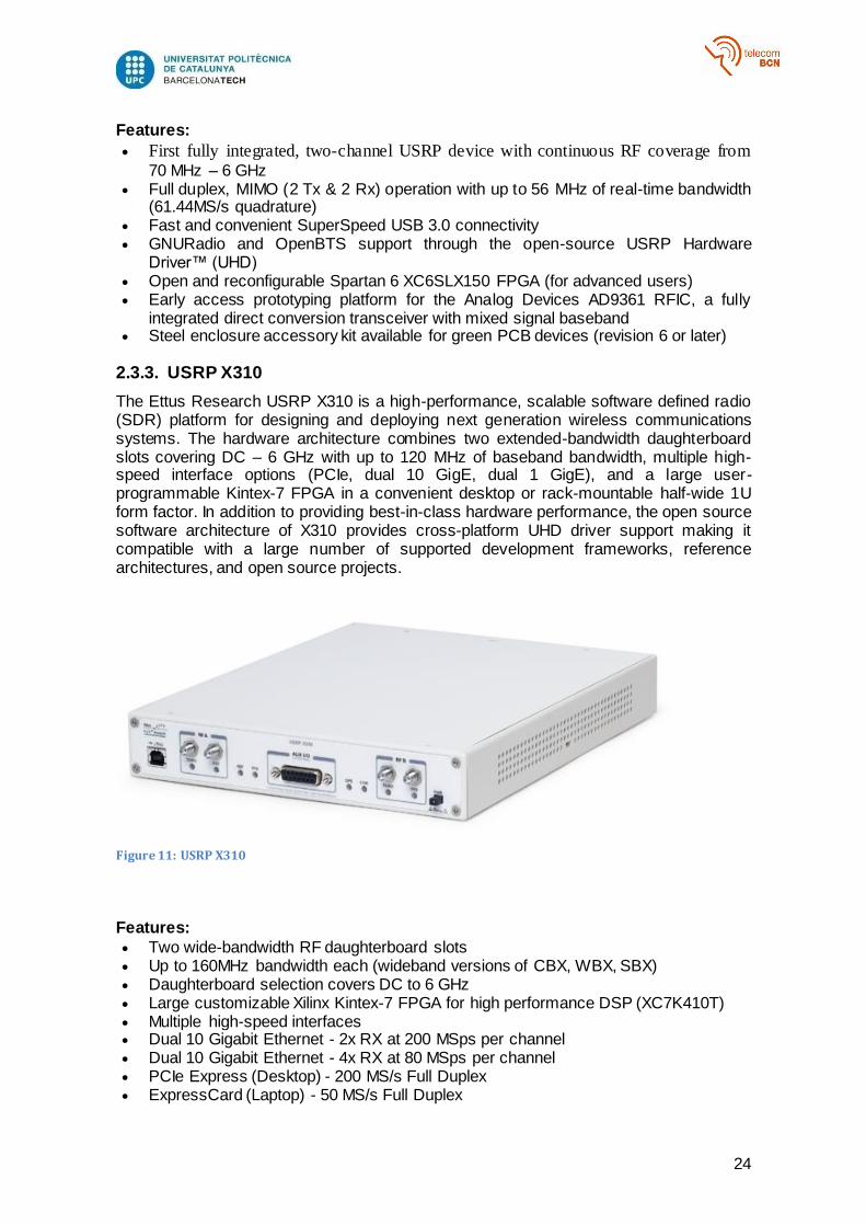
2.3.3. USRP X310

The Ettus Research USRP X310 is a high-performance, scalable software defined radio (SDR) platform for designing and deploying next generation wireless communications systems. The hardware architecture combines two extended-bandwidth daughterboard slots covering DC – 6 GHz with up to 120 MHz of baseband bandwidth, multiple high-speed interface options (PCIe, dual 10 GigE, dual 1 GigE), and a large user-programmable Kintex-7 FPGA in a convenient desktop or rack-mountable half-wide 1U form factor. In addition to providing best-in-class hardware performance, the open source software architecture of X310 provides cross-platform UHD driver support making it compatible with a large number of supported development frameworks, reference architectures, and open source projects.

Figure 11: USRP X310

Features:

Two wide-bandwidth RF daughterboard slots Up to 160MHz bandwidth each (wideband versions of CBX, WBX, SBX) Daughterboard selection covers DC to 6 GHz Large customizable Xilinx Kintex-7 FPGA for high performance DSP (XC7K410T) Multiple high-speed interfaces Dual 10 Gigabit Ethernet - 2x RX at 200 MSps per channel Dual 10 Gigabit Ethernet - 4x RX at 80 MSps per channel PCIe Express (Desktop) - 200 MS/s Full Duplex ExpressCard (Laptop) - 50 MS/s Full Duplex

25

Dual 1 Gigabit Ethernet - 25 MS/s Full Duplex UHD architecture provides compatibility with GNU Radio C++/Python API Amarisoft LTE 100 OpenBTS Other third-party software and frameworks Flexible clocking architecture Configurable sample rate Optional GPS-disciplined OCXO Coherent operation with OctoClock and OctoClock-G Compact and rugged half-wide 1U form factor for convenient desktop or rack mount

usage Digital I/O accessible on the front panel for custom control and interfacing from the

FPGA

2.3.4. NI USRP 2954R

10 MHz to 6 GHz, GPS-Disciplined OCXO, USRP Software Defined Radio Reconfigurable Device—The USRP-2954 provides an integrated hardware and software solution for rapidly prototyping high-performance wireless communication systems. Built on the LabVIEW reconfigurable I/O (RIO) architecture, USRP RIO delivers an integrated hardware and software solution, so researchers can prototype faster and shorten time to results. You can prototype a range of advanced research applications that include multiple input, multiple outputs (MIMO); synchronization of heterogeneous networks; LTE relaying; RF compressive sampling; spectrum sensing; cognitive radio; beamforming; and direction finding. The USRP-2954 is equipped with a GPS-disciplined 10 MHz oven-controlled crystal oscillator (OCXO) reference clock. The GPS disciplining delivers improved frequency accuracy and synchronization capabilities.

The same features of USRP X310

Figure 12: USRP 2954R

26

3. Methodology / project development:

This project has consisted on two well-depreciated parts (simulation and implementation),

plus a smaller part in the beginning for organization, understanding and study of the

required tools for the realization of the project. For the procedure, the tools Matlab and

Labview have been used.

3.1. Simulations

Matlab software has been employed entirely for the simulation part.

3.1.1. Communication Transmitter-Receiver

The first relevant part of the project consisted on the study of the system used for the

communication, meaning, it has been revised how the communication should be from the

beginning to the end.

The communication with two USRPs has been developed indoors, thus, it has been

decided and studied that the channel is a Rayleigh multipath, since it is the channel

which the best approach on an enclosed space with several objects inside.

Next, it has been decided to apply a BPSK modulation, since it is one of the simplest

communications; it also works correctly when transmitting data on the implementation in

the USRPs. The study of our protocol has resulted as follows:

Figure 13: Transmitter

Figure 14: Channel

BPSK

Modulator

Bits

01001110101010 Tx Filter

(root Raised Cosine)

X

cos(2𝜋 · 𝑓𝑐 · 𝑡 + 𝜑)

Rayleigh

Channel Multipath

𝑛𝑜𝑖𝑠𝑒

+

27

Figure 15: Receiver

To make this simulation, it has been required to design each and every one of the blocks, yet on a simple way, since it is not the main focus on this project and some gain blocks

have been omitted.

For some parts of the protocol/simulation, some functions already designed/implemented in the "Communications System Toolbox" have been used, such as the modulator/demodulator and the transmitter and receiver filters. Frequency, Multipath Rayleigh channel, channel estimation and the equalizer parts have been designed from

scratch.

3.1.1.1. Channel

To make the channel, the different paths to be traced by the signal have been designed,

indicating the delay and the gain on each path, being the first of all null.

Figure 16: Channel design

l

−cos(2𝜋 · 𝑓𝑐 · 𝑡+ 𝜑)

Rx Filter ( root Raised

Cosine)

Equalizer BPSK

Demodulator

Bits 01001110101010

X

28

Figure 17: Multipath/Rayleig channel

3.1.1.2. Channel estimation

For the channel estimation, it has been followed the simplest procedure. The transmitter

sends a signal known by the receiver. Therefore, to obtain the channel estimation, it is

made on the frequency domain, dividing the received signal with the sent one.

𝑦 = ℎ𝑐 ∗ 𝑥

𝑌 = 𝐻𝑐 · 𝑋 → 𝐻�̂� =𝑌

𝑋

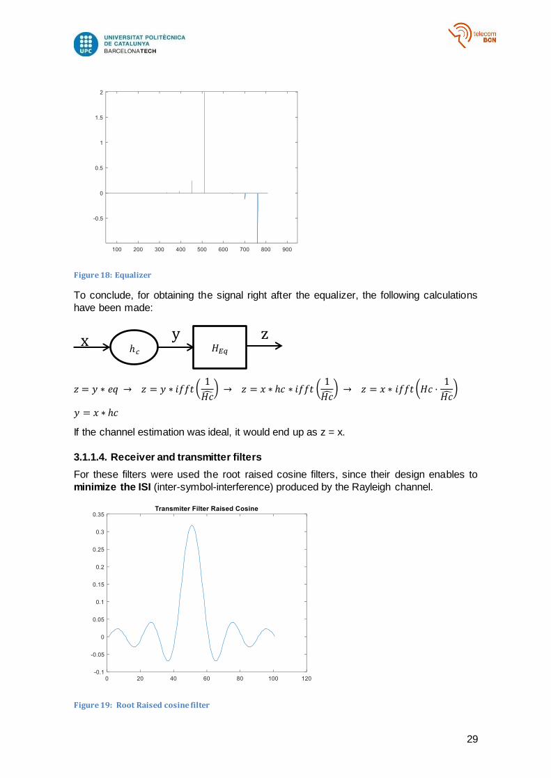
3.1.1.3. Equalizer

The equalizer has been obtained using the simplest method as well. The equalizer

consists on trying to arrange the signal, so as to make it resemble the most the sent

signal before the channel.

For this purpose, the equalizer has been designed as the inverse of the channel in the

frequency domain:

𝐻𝐸𝑞 =1

𝐻�̂�

29

Figure 18: Equalizer

To conclude, for obtaining the signal right after the equalizer, the following calculations

have been made:

𝑧 = 𝑦 ∗ 𝑒𝑞 → 𝑧 = 𝑦 ∗ 𝑖𝑓𝑓𝑡 (1

𝐻�̂�) → 𝑧 = 𝑥 ∗ ℎ𝑐 ∗ 𝑖𝑓𝑓𝑡 (

1

𝐻�̂�) → 𝑧 = 𝑥 ∗ 𝑖𝑓𝑓𝑡 (𝐻𝑐 ·

1

𝐻�̂�)

𝑦 = 𝑥 ∗ ℎ𝑐

If the channel estimation was ideal, it would end up as z = x.

3.1.1.4. Receiver and transmitter filters

For these filters were used the root raised cosine filters, since their design enables to

minimize the ISI (inter-symbol-interference) produced by the Rayleigh channel.

Figure 19: Root Raised cosine filter

ℎ𝑐 𝐻𝐸𝑞 x

y z

30

The raised cosine filter has been used on frequency, thus we have a sinc on time, with a

roll-off factor of 0.

3.1.2. Time of Arrival simulation (ToA)

In order to make this simulation, an algorithm has been designed to calculate the delay

on samples with the correlation method.

This simulation allows us to calculate the delay on samples, with a sampling frequency of

500 kHz, (used in the design of the channel as well), by the crossed correlation of the

signal which is sent and the received signal.

Once the crossed correlation is obtained, the first peak found on the correlation, in the index of that point, is the delay for the first path and, therefore, the delay on sample of

our signal. In order to find this peak, a threshold has been made by the "try and error"

method.

This method has been used since the first path of the channel is not always the one

carrying the most energy. If we focus only on the path with the highest power, it will

always give the correlation on the highest point, yet incorrectly, thus, one must focus on

the first peak which is not residual.

Figure 20: CrossCorrelation

Once these values are obtained, a simulation is made, where we introduce as input

parameter the channel through which we wish to transmit the signal (the input channel

corresponds only to the delays on time). Then, the algorithm to calculate the time in

seconds (as well as the distance) for our MS is:

𝑇 =1

𝑓𝑠

𝑠𝑒𝑔

𝑠𝑎𝑚𝑝𝑙𝑒

𝑑𝑒𝑙𝑎𝑦 = 𝑠𝑎𝑚𝑝 ∗ 𝑇 → 𝑑 = 𝑑𝑒𝑙𝑎𝑦 ∗ 𝑐

, being "c" the speed of transmission for the signal (3·108 m/s).

31

3.1.3. Positioning simulation

The last simulation which has been made is the trilateration method. It consists on

detecting and knowing the exact position of an object (mobile), using the ToA method.

This simulation consists on having 3 base stations and, by applying the ToA on each

base station with the mobile object, calculating the distance to each one of the base

stations. Then, on each BS (base station), it is calculated a circumference with the BS as

a centre and the obtained distance as the radius. The intersection point of the three

circumferences is where the exact position of the mobile is found.

3.2. Implementation

For this part of the implementation I have us the program named LabView. These

programs have been used to program the USRPs, the hardware used in this project and

for the correct sending and reception of the signals.

3.2.1. ToA

This implementation has been made only with LabView. The implementation has been

made with two USRP X301 and one USRP 2954R (they have the same features). The

scheme used to calculate the ToA is the following:

Figure 21: Model diagram

The software consists basically on sending a pulse from the BS and starting a timer. The

MS receives the pulse with a detector. Once it receives it, it resends it immediately to the

BS. Once the BS receives and detects correctly the pulse, it stops the timer. The total

time is T, while the ToA is:

𝑇 = 𝑡𝑝𝐵𝑠 + 2𝛥𝑡 + 𝑡𝑝𝑀𝑆 → 𝛥𝑡 =𝑇 − 𝑡𝑝𝐵𝑠 − 𝑡𝑝𝑀𝑆

2

, being T the total time it takes since the pulse is sent. T is the sum of processing time in

the BS, plus two times the time of the path and the processing time in the MS.

BS

USRP1

MS

USRP2

Tx1

Tx2

Rx2

Rx1

4.9GHz

5.9GHz

32

In order to do this program, it has been used the FDMA technique, since on the Uplink

(BS → MS) we have used a 4.9 GHz frequency and on the link Downlink (MS → BS) a

different frequency has been employed, of 5.9 GHz.

On the other hand, the TDMA technique could have been used, by applying different

time-slots to send and receive, since using the same frequency could cause interference

and inaccurate ToA calculus, as the signal could go from the sending antenna of the BS

the receiver antenna and generate a wrong value.

3.2.1.1. Base station

The LabView program made for this implementation has been the following:

Figure 22: BS Transmitter

Figure 22 shows the design used for the implementation of the BS transmitter, being able

to observe how the pulses are created (one imaginary and a real one), how the signal

synchronizes with the internal clock and how it is sent repetitively a pulse every 2000ms

(every 2 seconds).

Figure 23: BS Receiver 1

33

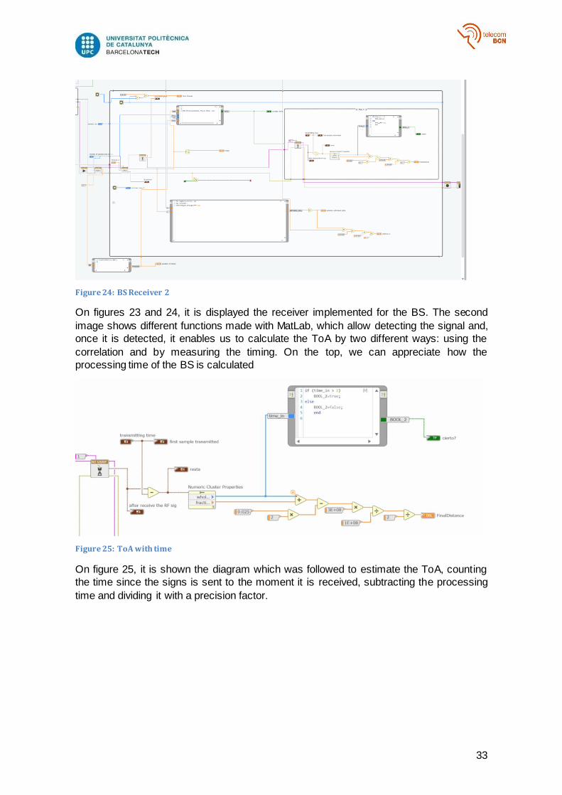
Figure 24: BS Receiver 2

On figures 23 and 24, it is displayed the receiver implemented for the BS. The second

image shows different functions made with MatLab, which allow detecting the signal and,

once it is detected, it enables us to calculate the ToA by two different ways: using the

correlation and by measuring the timing. On the top, we can appreciate how the

processing time of the BS is calculated

Figure 25: ToA with time

On figure 25, it is shown the diagram which was followed to estimate the ToA, counting

the time since the signs is sent to the moment it is received, subtracting the processing

time and dividing it with a precision factor.

34

Figure 26: ToA with correlation

Figure 26 exposes the followed procedure to calculate the ToA, the same way it has been

done on MatLab, with the correlation method and calculating the delay on samples.

3.2.1.2. Mobile station

Figure 27: MS receiver 1

Figure 27 contains the blocks diagram followed to the implementation of the MS receiver,

synchronizing it with the internal clock to revive the pulses.

Figure 28: MS receiver 2

35

This part of the receiver shows how the detector has been implemented with the first

pulse received.

Figure 29: MS transmitter

Figure 29 show how, once the pulse has been correctly detected, the transmitter

activates sending only one pulse to the BS immediately after the pulse has been

detected. It is also shown the processing time of the MS.

36

4. Results

4.1. Simulation Results

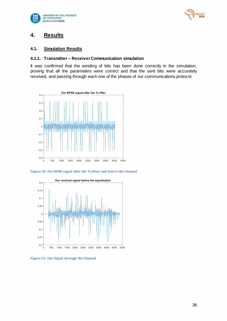
4.1.1. Transmitter – Receiver Communication simulation

It was confirmed that the sending of bits has been done correctly in the simulation,

proving that all the parameters were correct and that the sent bits were accurately

received, and passing through each one of the phases of our communications protocol.

Figure 30: Our BPSK signal after the Tx filter and before the channel

Figure 31: Our Signal through the Channel

37

Figure 32: Signal after the equalizer

On the figure 32 it is shown how the signal after the equalizer and the signal before

passing through the channel resemble a lot, thus, it is proven that the equalizer is

designed correctly.

Figure 33: Channel & Channel estimation

On the Figure 33 it is shown how the estimation of the channel is done properly, since we

have the different paths with different attenuations.

38

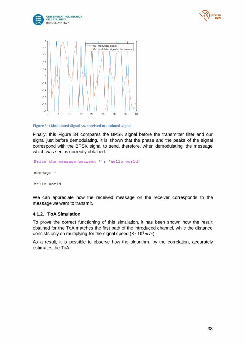
Figure 34: Modulated Signal vs. received modulated signal

Finally, this Figure 34 compares the BPSK signal before the transmitter filter and our

signal just before demodulating. It is shown that the phase and the peaks of the signal

correspond with the BPSK signal to send, therefore, when demodulating, the message

which was sent is correctly obtained.

We can appreciate how the received message on the receiver corresponds to the

message we want to transmit.

4.1.2. ToA Simulation

To prove the correct functioning of this simulation, it has been shown how the result

obtained for the ToA matches the first path of the introduced channel, while the distance

consists only on multiplying for the signal speed (3 · 108𝑚/𝑠).

As a result, it is possible to observe how the algorithm, by the correlation, accurately

estimates the ToA.

39

Figure 35: ToA simulation results

In the figure 35 it is shown how the ToA matches the first path of the introduced channel

as input parameter on our function (being null the first parameter of the channel, since the

signal does not travel directly).

Figure 36: Transmitted and received signal

On the figure 36, it is perceived how the delay on the samples, which has been produced

due to the channel, is of about 300 samples.

4.1.3. Position Simulation

To make this simulation, there were taken aleatory distances to two base stations and the

third distance to the third base station has been trigonometrically calculated. The

positions to the base stations have been set to our free will and this have been the results

of the simulation.

40

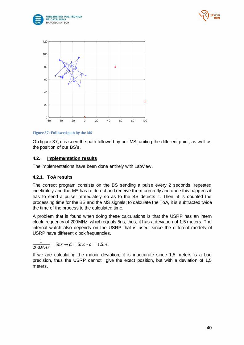
Figure 37: Followed path by the MS

On figure 37, it is seen the path followed by our MS, uniting the different point, as well as

the position of our BS’s.

4.2. Implementation results

The implementations have been done entirely with LabView.

4.2.1. ToA results

The correct program consists on the BS sending a pulse every 2 seconds, repeated

indefinitely and the MS has to detect and receive them correctly and once this happens it

has to send a pulse immediately so as to the BS detects it. Then, it is counted the

processing time for the BS and the MS signals; to calculate the ToA, it is subtracted twice

the time of the process to the calculated time.

A problem that is found when doing these calculations is that the USRP has an intern

clock frequency of 200MHz, which equals 5ns, thus, it has a deviation of 1,5 meters. The

internal watch also depends on the USRP that is used, since the different models of

USRP have different clock frequencies.

1

200𝑀𝐻𝑧= 5𝑛𝑠 → 𝑑 = 5𝑛𝑠 ∗ 𝑐 = 1,5𝑚

If we are calculating the indoor deviation, it is inaccurate since 1,5 meters is a bad

precision, thus the USRP cannot give the exact position, but with a deviation of 1,5

meters.

41

4.2.1.1. Base station

Figure 38: BS transmitter Panel

Figure 38 shows all the parameters of our BS, used to calculate the ToA

Figure 39: BS receiver panel

All the parameters of our receiver are observed on figure 39, as well as a graphic where

appears the received signal (on this case, it is only receiving noise). The most relevant

part of this image is the “FinalDistance”, referring to the distance on meters after having

calculated the ToA and multiplied it by the transmission speed; on this occasion, we use

a distance of 44cm.

42

4.2.1.2. Mobile station

Figure 40: MS receiver panel

On figure 40 appear all the parameters of the receiver for the MS, which have been used

for calculating the ToA. It is also seen a graphic of the received signal (on this case, only

noise).

Figure 41: MS transmitter panel

Finally, figure 41 shows the transmitter and its parameters, which have been used for

calculating the ToA, via the USRP.

43

5. Budget

To complete this work, USRP devices are required, as well as the software Matlab and Labview. Here are listed the prices for each device, as well as for the license of the

software.

-USRP B205mini 910 €

-USRP B210 1216 €

-USRP X310 5290 €

-NI USRP 2954R 7128 €

-VERT2450 Antenna 40 € x 4 = 160 €

-Matlab 2000 €

-LabView 3451 €

The total sum is approximately 20155 € on components and software. As for timing, 8 hours, five days a week were dedicated in order to make this project possible, which

should be evaluated with a cost of 8 €/hour.

44

6. Conclusions and future development:

The next step for a future development or the continuation of this project is the use of 3

BS, using the same method to calculate the ToA of the three BS with the MS and then,

just as it has been made on the simulation, using the method of trilateration to calculate

the exact position of the MS on real time.

Another procedure to which one could improve is using a USRP with a higher clock

frequency, so that the precision when calculating the ToA is enhanced.

Another possible improvement could be the amelioration of the existing code, searching

for more efficient algorithms to calculate the ToA; also, the use of productive methods to

locate a MS, such as using together the ToA and AoA (Angle of Arrival) methods, which

in general only employs one BS with an array of antennas.

To conclude, this part of the project has been developed for its use in a future on

applications for the localization of drones on real time, where a drone would be the MS.

45

Bibliography:

[1] [1] Overview of Radiolocation in CDMA Cellular Systems - James J. Caffery, Jr. and Gordon L. Stüber Georgia Institute of Technology

[2] [2] R. Jurgen, “The Electronic Motorist,” IEEE Spectrum, vol. 32, Mar. 1995, pp. 37–48

[3] [3] M. Vossiek , L. Wiebking , P. Gulden , J. Wieghardt , C. Hoffmann , and P. Heide , “ Wireless local positioning , ” I EEE Microw. Mag. , vol. 4 , no. 4 , pp. 77 – 86 , 2003 .

[4] [4] S. Capkun , M. Hamdi , and J. P. Hubaux , “ GPS - free positioning in mobile ad – hoc networks , ” Proc. 34th Annual Hawaii International Conference on System Science , Maui, Hawaii, Jan. 3 – 6, 2001 .

[5] [5] T. S. Rappaport , J. H. Reed , and B. D. Woerner , “ Pos ition location using wireless communications on highways of the future , ” IEEE Communication Magazine , pp. 33 – 41 , Oct. 1996 .

[6] [6] M. Laoufi , M. Heddebaut , M. Cuvelier , J. Rioult , and J. M. Rouvaen , “ Positioning emergency calls along roads and motorways using a GSM dedicated cellular radio network , ” Proc. IEEE Vehicular Technology Conference , vol. 5, pp. 2039 – 2046 , Sep. 24 – 28, 2000 .

[7] [7] U. - H. Kim , J. Kim , D. Kim , H. Kim , and B. - J. You , “ Speaker localization on a humanoid robot ’ s head using the TDOA - based feature matrix , ” Proc. IEEE 17th International Symposium on Robot and Human Interactive Communication , Munich, Germany, pp. 610 – 615 , Aug. 1 – 3, 2008 .

[8] [8] N. Alsindi , L. Xinrong , and K. Pahlavan , “ Analysis of time of arrival estimation using wideband measurements of indoor radio propagations , ” IEEE Trans. Instrum. Meas. , vol. 56 , no. 5 , pp. 1537 – 1545 , 2007 .

[9] [9] W. Xu and S. A. Zekavat , “ Spatially correlated multi - user channels: LOS versus NLOS , ” Proceedings IEEE DSP/SPE workshop 2009 , Florida, Jan. 4 – 7, 2009 .

[10] [10] Z. Wang , W. Xu , and S. A. Zekavat , “ A novel LOS and NLOS localization technique , ” Proceedings IEEE DSP/SPE workshop 2009 , Florida, Jan. 4 – 7, 2009 .

[11] [11] M. Omerbashich , “ Integrated INS/GPS navigation from a popular perspective , ” J. Air Transport. , vol. 7 , no. 1 , pp. 103 – 118 , 2002 .

[12] [12] J. Werb and C. Lanzl , “ Designing a positioning system for fi nding things and people indoors , ” IEEE Spectr. , vol. 35 , no. 9 , pp. 71 – 78 , 1998 .

[13] [13] L. M. Ni , Y. Liu , Y. C. Lau , and A. P. Patil , “ LANDMARC: indoor location sensing using active RFID , ” Wireless Networks , vol. 10 , pp. 701 – 710 , 2004 .

[14] [14] W. Wang and S. A. Zekavat , “ Comparison of semi - distributed multi - node TOA - DOA fusion localization and GPS - aided TOA (DOA) fusion localization for manets , ” EURASIP J. Adv. Signal Process. , vol. 2008. Article ID 439523, 16 pages, 2008 . doi:10.1155/2008/439523.

[15] [15] W. Wang and S. A. Zekavat , “ A novel semi - distributed localization via multi - node TOA – DOA fusion , ” IEEE T. Veh. Technol. , vol. 58 , no. 7 , pp. 3426 – 3435 , 2009 .

[16] [16] S. G. Ting , O. Abdelkhalik , and S. A. Zekavat , “ Differential geometric estimation for spacecraft formations orbits via a novel wireless positioning , ” Proceedings IEEE Aerospace Conference , 2010 .

[17] [17] T. Williamson and N. A. Spencer , “ Development and operation of the traffi c alert and collision avoidance system (TCAS) , ” IEEE Control Syst. Mag. , vol. 77 , no. 11 , pp. 1735 – 1744 , 1989 .

[18] [18] J. Hightower and G. Borriello , “ Location systems for ubiquitous computing , ” Computer , vol. 34 , no. 8 , pp. 57 – 66 , 2001 .

[19] [19] P. Bahl and V. N. Padmanabhan , “ Radar: an in - building RF - based user - location and tracking system , ” Proc. IEEE INFOCOM 2000 , Tel Aviv, Israel, vol. 2, pp. 775 – 784 , Mar. 2000.

[20] [20] K. Saneyoshi , “ Drive assist system using stereo image recognition , ” Proc. IEEE Intell. Veh. Symp. , pp. 230 – 235 , 1996 .

[21] [21] S. A. Zekavat , A. Kolbus , X. Yang , Z. Wang , J. Pourrostam , and M. Pourkhaatoon , “ A novel implementation of DOA estimation for node localization on software defi ned radios: achieving high performance with low complexity , ” Proceedings IEEE ICSPC 2007 , Dubai, UAE, 26 – 27 Nov. 2007 .

[22] [22] J. Pourrostam , S. A. Zekavat , and H. Tong , “ Novel direction - of - arrival estimation techniques for periodic sense local positioning systems in wireless environment , ” Proceedings IEEE Radar ’ 07 , 17 – 20 April, 2007 , Boston.

[23] [23] J. Pourrostam , S. A. Zekavat , and H. Tong , “ Novel direction - of - arrival estimation techniques for periodic sense local positioning systems in wireless environment , ” Proceedings IEEE Radar ’ 07 , 17 – 20 April, 2007 , Boston.

46

Glossary

- MS: Mobile Station

- BS: Base Station

- RTLS: Real Time Locating Systems

- RFID: Radio Frequency Identification

- GPS: Global Positioning System

- UAV: Unnamed aerial vehicle

- SDR: Software-Defined Radios

- USRP: Universal Software Radio Peripheral

- ToA: Time of Arrival

- AoA: Angle of Arrival

- LPS: Local Positioning System

- INS: Inertial Navigation System

- TDOA: Time Difference of Arrival

- RSSI: Received Signal Strength Indicator

- RSS: Received Signal Strength

- LOS: Line of Side

- NLOS: No Lone od Side

- WLPS: Wireless Local Positioning System

- TCAS: Traffic Collision Avoidance System

- WLAN: Wireless Local Area Network

- NIC: Network Interface Card

- RADAR: Radio Detection and Ranging

- NI: National Instruments

- RF: Radio Frequency

- MIMO: Multiple In Multiple Out