
COMMONWEALTH OF AUSTRALIA - University of Queensland · They have since been corrected and mod-ied...
73
COMMONWEALTH OF AUSTRALIA Copyright Regulations 1969 WARNING This material has been reproduced and communicated to you by or on behalf of the University of Queensland pursuant to Part VB of the Copyright Act 1968 (the Act). The material in this communication may be subject to copyright under the Act. Any further reproduction or communication of this material by you may be the subject of copyright protection under the Act. Do not remove this notice.
Transcript of COMMONWEALTH OF AUSTRALIA - University of Queensland · They have since been corrected and mod-ied...

COMMONWEALTH OF AUSTRALIA
Copyright Regulations 1969
WARNING
This material has been reproduced and communicated to you by or on behalf of the University of Queensland pursuant to Part VB of the Copyright Act 1968 (the Act). The material in this communication may be subject to copyright under the Act. Any further reproduction or communication of this material by you may be the subject of copyright protection under the Act. Do not remove this notice.


PHYS3020 — Statistical Mechanics 2006
http://www.physics.uq.edu.au/people/mdavis/phys3020/
Matthew Davis
Acknowledgement
These notes were first prepared by Joel Gilmore, Kevin Brake, and Mark Dowling, based on RossMcKenzie’s handwritten notes for PHYS3020 in 2001. They have since been corrected and mod-ified by Matthew Davis (2004–6). Thanks to Amanda Beasley for an extensive list of typos in2004.
Very Important
These notes are not complete, are not a substitute for the textbook, and are not a substitute forattending lectures.
The material outlined herein will be covered in greater detail in lectures and tutorials.
While care has been taken to ensure the accuracy of these notes, there will undoubtedly be errors,which will be picked up and corrected during class.
1

2

What is the goal of statistical mechanics?
Quick answer: to traverse from the microscopic to the macroscopic using statistical methods.
E.g. from describing the physics of individual atoms to that of bulk matter in the form of gases,liquids, solids.
Thermodynamics describes the macroscopic properties of matter without any reference to the mi-croscopic atoms and molecules that make up a particular system. It places restrictions on trans-formations of these properties that seem to be universal. However, it gives us no insight into whythese restrictions exist.
Theoretically, if we know the forces that act between the atoms and molecules that make up athermodynamic system, we can write down and solve the equations of motion for every particle(either using quantum mechanics or classical mechanics). However, it is obviously impractical todo so, and usually we aren’t interested in the detailed dynamics of every particle. However weare interested in the bulk thermodynamics properties such as pressure and temperature that weare familiar with from everyday life. We can obtain these using the laws of quantum or classicalmechanics combined with statistics. For example : later in the course we will show that classicalnon-interacting particles obey the ideal gas law, PV = NkBT .
Statistical mechanics has a wide range of applications from condensed matter to astrophysics toquantum optics. Some that we will consider are:• Cosmic microwave background• White dwarf stars• “Unzipping” DNA• Electronic properties of metals• Magnetic phase transitions• Bose-Einstein condensation
Some fundamental questions
Most importantly — the second law of thermodynamics.• Why does heat disperse as time passes?• Why does time seem to flow in only one direction?Explicitly, the microscopic equations of motion are time reversal invariant. e.g. Newton’s equationof motion for all N atoms in a gas
md2~ri
dt2= ~Fi(~r1, ~r2, . . . , ~rN)
are invariant under the transformation t → −t.
3

Hamilton’s equations of motion
pi = −∂H
∂qi
, qi =∂H
∂pi
,
are invariant under t → −t, pi → −pi, pi → −pi, qi → −qi. However, the behaviour of macro-scopic objects is not time reversal invariant. Have you ever seen• water go up a waterfall?• a fresh cup of tea get hotter and not colder with time?• sugar “undissolve” itself from the same cup of tea?The fact that playing a video tape backwards makes (some of) us laugh within seconds demon-strates that the macroscopic world is irreversible — time flows in one direction.
Significance
Statistical mechanics has played a crucial role in the history of physics. In particular it is at theheart of• the atomic hypothesis• the proposal of the quantum by Planck• even the origin of the universe! (via the observation of the cosmic microwave background)
Course summary
You may remember that the areas of classical mechanics, quantum mechanics, general relativity,and electromagnetism can be summarised by just a few equations. It turns out that statisticalmechanics can be as well.
Consider a closed system at constant temperature T , volume V . Enumerate all of the possible mi-croscopic configurations of the system by i, with Ei the energy of the ith state. Then the Helmholtzfree energy F (V, T ) is related to the partition function via
exp(−F/kBT ) = Z ≡∑
i
exp(−Ei/kBT )
where kB = 1.381 × 10⁻²³ J/K = R/NA is Boltzmann’s constant. This relates the macroscopicpotential F (V, T ) to our microscopic knowledge of the system.
This course is concerned with
1. Deriving this result, along with variations on it for e.g. variable particle number N .
2. Applying this result to obtain (and hopefully understand!) the thermodynamic properties ofa large number of model systems.
4

N.B. It turns out that enumerating the microstates, finding their energies and performing the sumis almost always a highly non-trivial exercise!
However, before we get stuck into statistical mechanics, we will use the first couple of lectures ofthis course reviewing what you should remember from thermodynamics.
5

Problem solving strategy
It is easy to get lost sometimes when approaching a problem in statistical mechanics — it happensto everyone. The strategy described below applies to just about every problem that we will comeacross in this course, and should help you get started if you are stuck.
1. Define the system. What are the macrostates?
2. Which ensemble is appropriate: microcanonical, canonical or grand canonical?
3. What are the microstates? This means working out what are the quantum numbers of thesystem, their associated energies, and the degeneracies of each energy.
4. Evaluate the partition function: i.e. perform the sum.
5. You now have the free energy. From its derivatives you can find thermodynamic propertiessuch as the internal energy, entropy, and pressure (equation of state).
6. What is the relevant microscopic energy scale? Usually it is the energy level spacing. Call itε0, say.
7. Consider the high temperature limit kBT ε0. This is the classical regime. Do your resultsagree with the equipartition theorem?
8. Consider the low temperature limit kBT ε0. This is the quantum regime. Do your resultsfor the entropy agree with the third law of thermodynamics?
6

Some useful things to know
Often in statistical mechanics we run into formulae that are somewhat complicated and difficult towork with. Often, this can be circumvented by making a well-chosen approximation. An impor-tant skill to develop in PHYS3020 is an understanding of when and where such approxima-tions can be made. It is also very important to check whether your results make physical sense.For example, at high temperature is your result consistent with what you know about classicalphysics?
Here we describe a few useful tools that will that turn up time and time again.
Taylor series expansion and exponentials
The Taylor expansion or series of the function f(x) about the point a is as follows
f(x) = f(a) + (x − a)f ′(a) +1
2(x − a)2f ′′(a) +
1
6(x − a)3f ′′′(a) + . . . (1)
=∞∑
n=0
(x − a)n
n!
dnf(x)
dxn
∣
∣
∣
∣
x=a
(2)
Taylor series are often taken about the origin, which makes them look somewhat simpler. Probablythe most important Taylor series for use in statistical mechanics is that for ex where
ex = 1 + x +x2
2!+
x3
3!+
x4
4!+ . . . (3)
If |x| 1 then we can often truncate this series at the first term
e±x ≈ 1 ± x. (4)
Understand how big things are
It is very important to understand the importance of various terms in different physical situations,and make approximations based on this knowledge. If we have an expression like 1 + x, we canforget the x if it is very small. However, if it is very large then we can probably drop the one.
As an example, exponentials often turn up in the form (eε/kBT − 1). So when we have ε kBTthen we can approximate this as
(eε/kBT − 1) ≈(
1 +ε
kBT
)
− 1,
≈ ε
kBT. (5)
In the other limit when ε kBT , then the exponential term is going to be very large compared toone, so we can use
(eε/kBT − 1) ≈ eε/kBT . (6)
7

Changing variables
A lot of integrals turn up in statistical mechanics, and with all the terms involved they can be quiteconfusing. A strategy that is often useful is to make a change of variables so that you can see theintegral in its simplest form. An example is for the energy density of a hollow box d
U
V=
∫ ∞
0
8π
(hc)3
ε3
eε
kBT − 1dε (7)
If we change variables to x = ε/kBT it becomes
U
V=
8π (kBT )4
(hc)3
∫ ∞
0
x3 dx
ex − 1(8)
This now has the advantage that all the parameter dependence is outside the integral, which is justsome constant. We can look this up in tables — we find that it is π4/15, and the final result is
U
V=
8π5 (kBT )4
15 (hc)3 (9)
Changing variables can also be useful when considering the relative importance of terms.
Stirling’s approximation
Another useful approximation is for N ! when N is very large. Factorials turn up quite oftenwhen working out different arrangements of particles in the microcanonical ensemble. Stirling’sapproximation can make such terms easier to deal with. We have
N ! ≈(
N
e
)N √2πN. (10)
This result is derived in Appendix B of Schroeder. Usually we want to know the logarithm offactorials: then we can use the slightly less accurate
ln N ! ≈ N ln N − N. (11)
Some useful integrals
∫ ∞
0
x3 dx
ex − 1=
π4
15, (12)
∫ ∞
−∞
e−ax2
dx =
√
π
a. (the gaussian integral) (13)
8

Chapter 1
Review of thermodynamics
Thermodynamics is a phenomenological theory of matter. It should really be called thermostatics.It describes systems in equilibrium, i.e., systems which when left to themselves are such that largescale observations of them do not reveal any changes with time.
Thermodynamics
• makes no assumptions about the microscopic (atomic) nature of matter.
• gives general relations between measurable quantities such as specific heats and compress-ibilities, e.g.
(
∂V
∂T
)
P
= −(
∂S
∂P
)
T
,dP
dT=
L
T∆V
• does not say why these quantities have the values that they do.
1.1 Basics
• A thermodynamic system is any macroscopic system that can be defined by a finite numberof co-ordinates, or thermodynamic parameters. Some examples are given in Figures 1.1, 1.2,1.3.
• Thermodynamic parameters are measurable macroscopic quantities associated with they
V P
Figure 1.1: Gas cylinder with moveable piston
9
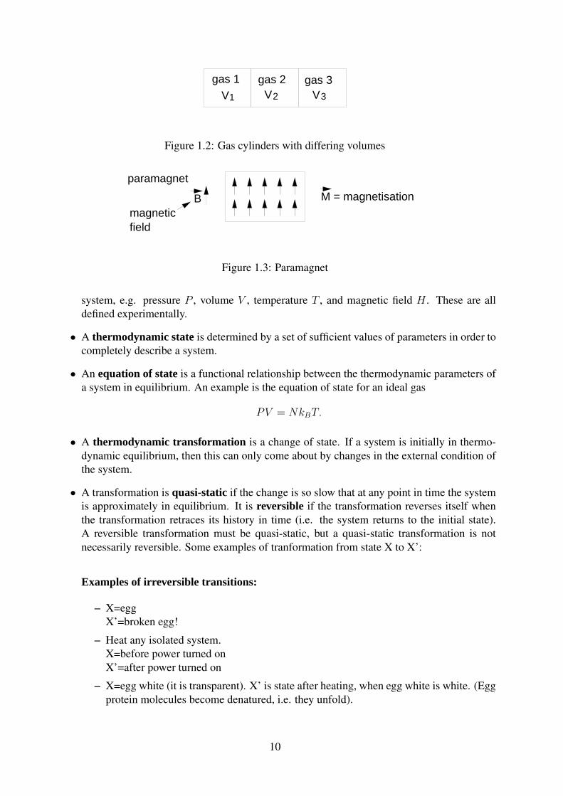
gas 1 gas 2 gas 3V1 V2 V3
Figure 1.2: Gas cylinders with differing volumes
paramagnet
magnetic field
B M = magnetisation
Figure 1.3: Paramagnet
system, e.g. pressure P , volume V , temperature T , and magnetic field H . These are alldefined experimentally.
• A thermodynamic state is determined by a set of sufficient values of parameters in order tocompletely describe a system.
• An equation of state is a functional relationship between the thermodynamic parameters ofa system in equilibrium. An example is the equation of state for an ideal gas
PV = NkBT.
• A thermodynamic transformation is a change of state. If a system is initially in thermo-dynamic equilibrium, then this can only come about by changes in the external condition ofthe system.
• A transformation is quasi-static if the change is so slow that at any point in time the systemis approximately in equilibrium. It is reversible if the transformation reverses itself whenthe transformation retraces its history in time (i.e. the system returns to the initial state).A reversible transformation must be quasi-static, but a quasi-static transformation is notnecessarily reversible. Some examples of tranformation from state X to X’:
Examples of irreversible transitions:
– X=eggX’=broken egg!
– Heat any isolated system.X=before power turned onX’=after power turned on
– X=egg white (it is transparent). X’ is state after heating, when egg white is white. (Eggprotein molecules become denatured, i.e. they unfold).
10

remove partition
air
O2N2
(N ,O Mixture)2 2
x
x
Figure 1.4: Mixing of gases N2 and O2 by removing partition
H O2
Figure 1.5: Heating of water
Example of a reversible transition:
V Pgasmoveable piston
Figure 1.6: Transformation is reversible if system is thermally isolated and piston is moved slowlyenough (i.e. process is quasi-static.)
• The concept of work is taken over from mechanics. For a system with parameters P , V , andT the work done on the system is
dW = −PdV.
• Heat is absorbed by a system if its temperature increases yet no work is done. The heatcapacity C is defined by
∆Q = C∆T
where ∆Q is the heat absorbed and ∆T is the change in temperature. The heat capacitydepends on how the system is heated, e.g. at constant volume or constant pressure. Heatcapacities per unit mass or per mole are called specific heats, and are denoted by a lowercase c.
11

• A heat reservoir (or simply reservoir) is a system so big that any loss or gain in heat doesnot change its temperature.
• A system is thermally isolated if no heat exchange can take place between it and the restof the world. Any transformations that occur without the transfer of heat are said to beadiabatic.
• Extensive thermodynamic quantities are proportional to the amount of substance that makesup a system. Examples are particle number N , volume V . Intensive quantities are indepen-dent of the amount of substance, e.g. temperature T , pressure P .
From this point we move on to the laws of thermodynamics. The historical development of these isquite interesting, and if you have the time you should read the popular book by H. C. von Baeyer,Warmth disperses and time passes: the history of heat, library QC318.M35 V66 1999. However,here we will make do with a practical summary.
The laws of thermodynamics may be considered as mathematical axioms defining a mathematicalmodel. It is possible to deduce the logical consequences of these, and it remarkable how much canbe derived from very simple assumptions. If you are interested in this approach try reading H.A.Buchdahl, Twenty Lectures on Thermodynamics (Permagon, 1975), library QC311.B9155 1975.
It should be remembered that this model is purely empirical, and does not rigorously correspondto the real world. In particular it ignores the atomic structure of matter, so it will inevitably failin the atomic domain. However, in the macroscopic world thermodynamics is extremely powerfuland useful. It allows one to draw both precise and far reaching conclusions from a few seeminglycommonplace observations.
1.2 The Second Law and Entropy
A good many times I have been present at gatherings of people who, by the stan-dards of the traditional culture, are thought highly educated and who have with con-siderable gusto been expressing their incredulity at the illiteracy of scientists. Onceor twice I have been provoked and have asked the company how many of them coulddescribe the Second Law of Thermodynamics. The response was cold: it was alsonegative. Yet I was asking something which is about the scientific equivalent of: Haveyou read a work of Shakespeare’s?— C.P. Snow, The Two Cultures (Cambridge University Press, Cambridge, 1959).
We can order all the states of a system according to whether they are adiabatically accessible toone another.
X → X ′ → X ′′
This ordering defines an empirical entropy function, S(X). The second law can be written:
The entropy of the final state of an adiabatic transition is never less than that of theinitial state i.e. dS ≥ 0.
12

N.B. S(X) is not uniquely defined. If f(S) is a monotonically increasing function then f(S(X))is equally appropriate as an empirical entropy function. It doesn’t require the definition of heat ortemperature.
1.2.1 Statements of the second law
Kelvin: There exists no thermodynamic transformation whose sole effect is to extract a quantityof heat from a given heat reservoir and to convert it entirely into work.
Claussius: There exists no thermodynamic transformation whose sole effect is to extract a quantityof heat from a colder reservoir and deliver it to a hotter reservoir.
The key word in both of these statements is sole!
1.3 The First Law, Internal Energy, and Heat
In a mechanical system with conservative forces the energy of the equilibrium state only dependson the co-ordinates x1, x2, x3, ..., xN and not on the history of the system. This allows definitionof a potential energy function V (x1, x2, x3, ..., xN )
The First Law of Thermodynamics∼
The amount of work done by a system in an adiabatictransition depends only on the co-ordinates of
the final state.
As a result we can define an Internal Energy Function, U , which has the property that the workW0 done by a system in an adiabatic transition is equal to the decrease −∆U of its internal energy.
0 = W0 + ∆U
Suppose the system K is no longer adiabatically isolated and undergoes a transition from state Xto X’. In general, we expect W0 + ∆U 6= 0. The new quantity
Q = W + ∆U
is called the heat absorbed by K.
For an infinitesimal transformation the first law can be written
dU = dQ + dW (1.1)
It should be remembered that dQ and dW considered individually are inexact differentials — i.e.they depend on the path of the transformation. However, dU itself is an exact differential, whichmeans that it has a unique value for a particular thermodynamic state.
13

A trivial consequence of the first law is that no heat is exchanged in an adiabatic process.
Example:
room temperature
V
ice water
Figure 1.7: Thermos of ice water
Thermos of ice water with heating element, as shown in Figure 1.7Initial state X = ice waterFinal state X’ = boiling waterProcess 1: lid of thermos is on so system is adiabatically isolated. Electrical work done to get fromX to X’ does not depend on the time taken. Eg. apply a small current a long time or a large currentfor a small time or turn off the current every now and then.Process 2: lid of thermos is off so the system is not adiabatically isolated. Work done does dependon history. Eg. if we wait a few hours before turning on the current the ice melts and less work isrequired compared to if we quickly turn on a large current to get from X to X’.
1.4 The Zeroth Law
Two systems KA and KB are said to be in equilibrium with one another if when they are broughtinto thermal contact the states they are in do not change.
The Zeroth Law of Thermodynamics∼
If each of two systems are in equilibrium witha third system then they are in equilibrium
with one another (Figure 1.8)
This allows us to define an empirical temperature function, t. Like an empirical entropy functionis any function that always increases, an empirical temperature function is any value that is the
14
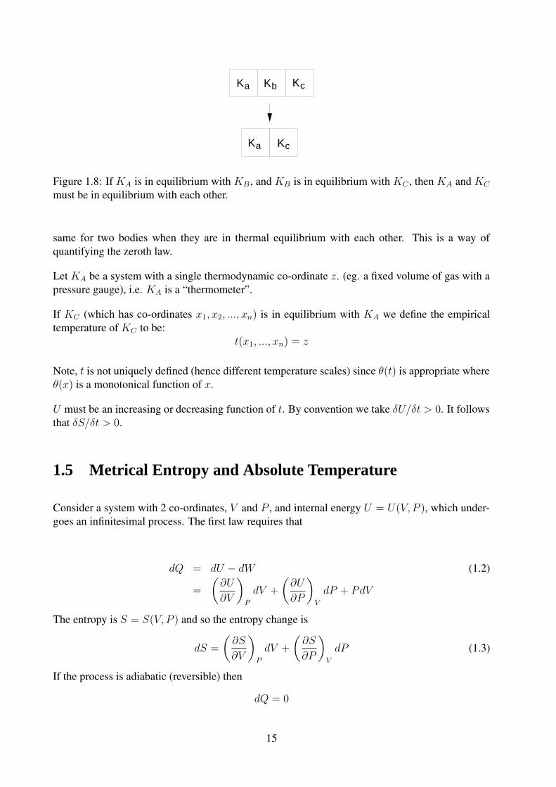
Ka Kb KcKc
Ka Kc
Figure 1.8: If KA is in equilibrium with KB, and KB is in equilibrium with KC , then KA and KC
must be in equilibrium with each other.
same for two bodies when they are in thermal equilibrium with each other. This is a way ofquantifying the zeroth law.
Let KA be a system with a single thermodynamic co-ordinate z. (eg. a fixed volume of gas with apressure gauge), i.e. KA is a “thermometer”.
If KC (which has co-ordinates x1, x2, ..., xn) is in equilibrium with KA we define the empiricaltemperature of KC to be:
t(x1, ..., xn) = z
Note, t is not uniquely defined (hence different temperature scales) since θ(t) is appropriate whereθ(x) is a monotonical function of x.
U must be an increasing or decreasing function of t. By convention we take δU/δt > 0. It followsthat δS/δt > 0.
1.5 Metrical Entropy and Absolute Temperature
Consider a system with 2 co-ordinates, V and P , and internal energy U = U(V, P ), which under-goes an infinitesimal process. The first law requires that
dQ = dU − dW (1.2)
=
(
∂U
∂V
)
P
dV +
(
∂U
∂P
)
V
dP + PdV
The entropy is S = S(V, P ) and so the entropy change is
dS =
(
∂S
∂V
)
P
dV +
(
∂S
∂P
)
V
dP (1.3)
If the process is adiabatic (reversible) then
dQ = 0
15

The second law also requiresdS = 0
It follows that there must exist some function λ(V, P ) such that
dQ = λdS.
Proof
Setting dQ = 0 in Eq. (1.3) requires
dP =−1(
∂U∂P
)
V
(
P +
(
∂U
∂V
)
P
)
dV
substituting this into Eq. (1.3) gives
dS =
[
(
∂S
∂V
)
P
−(
∂S∂P
)
V(
∂U∂P
)
V
(
P +
(
∂U
∂V
)
P
)
]
dV.
We can only have dS = 0 ifP +
(
∂U∂V
)
P(
∂U∂P
)
V
=
(
∂S∂V
)
P(
∂S∂P
)
V
It follows (from Equation 1.3) that
dS(
∂S∂P
)
V
=
(
∂S∂V
)
P(
∂S∂P
)
V
dV + dP
=
(
P +(
∂U∂V
)
P
)
(
∂U∂P
)
V
dV + dP
=1
(
∂U∂P
)
V
dQ
λ(V, P ) =
(
∂U∂P
)
V(
∂S∂P
)
V
We now show that λ can only depend on the empirical temperature, t. Consider a system, C,composed of two parts, A and B, as shown in Figure 1.9.
For any infinitesimal process (SA and SB are the empirical entropy)
dQC = dQA + dQB
λCdSC = λAdSA + λBdSB
dSC =λA
λC
dSA +λB
λC
dSB
16

A B
C
t = t = t = tA B C
Figure 1.9: System C
Thus SC can only be a function of SA and SB . The same applies to λA
λCand λB
λC. But, the only
co-ordinate of B on which λA can depend is t. This makes sense if
λA = T (t)fA(SA)
λB = T (t)fB(SB)
λC = T (t)fC(SA, SB)
we define the metrical entropy asSA =
∫
fA(SA)dSA
so that
dQA = λAdSA
= TfA(SA)dSA
= TdSA
andSC = SA + SB
T (t) is the absolute temperature function. S is the metrical entropy and is characterised by itsadditivity (above). It is an extensive property, as are U and V , i.e., if the system size is doubled
V −→ 2V, S −→ 2S, U −→ 2U
Temperature and pressure are intensive properties, i.e., if the system size is doubled
V −→ 2V, T −→ T, P −→ P
For an infinitesimal processdQ = TdS = dU + PdV
Hence1
T=
(
∂S
∂U
)
V
1.6 The Third Law
Ref. Schroeder, p. 92–5.
Experimentally, one finds
17

1. All heat capacities, CV (T ) = (∂U/∂T )V , go to zero as T → 0, at least as fast as T → 0.
2. It is not possible to cool any system to T = 0.
Consequences
A) The first condition ensures the convergence of the integral
S(T, V ) − S(T = 0, V ) =
∫ T
0
dQ
T=
∫ T
0
(
∂U
∂T
)
V
dT
T=
∫ T
0
CV (T )
TdT
Hence, we have (∂S/∂T )V → 0 as T → 0.
B) Consider a reversible adiabatic process in which T and V vary.
0 = dS =
(
∂S
∂T
)
V
dT +
(
∂S
∂V
)
T
dV
Substituting in that (∂S/∂T )V = CV (T )/T , we see that
⇒ dT
dV=
−T
CV (T )
(
∂S
∂V
)
T
If (∂S/∂V )T is non-zero as T → 0 then (dT/dV ) > 0 is non-zero, so by increasing V wecan cool the system right the way to T = 0. As this is not possible experimentally, we musthave (∂S/∂V )T → 0 as T → 0.
These two points show that the gradient of the entropy tends to zero as T → 0. This be summarisedin the
Third Law of Thermodynamics∼
The entropy function has the same finite value for all states which have T = 0
Because entropy is only defined up to an additive constant (like internal energy), we can set thisequal to zero.
1.7 Free Energy Tends to Decrease
Ref. Schroeder, p. 161-2.
For an isolated system, the entropy tends to increase, i.e., the equilibrium state is such that S(U, V,N)is a maximum. However, what about a system connected to a heat reservoir?
18

R
K
Figure 1.10: System K in equilibrium with reservoir R
Consider a system, K, at constant temperature, T , with fixed V and N , and in equilibrium with anenvironment (reservoir), R, which is also at fixed V and N .
For an infinitesimal process
dStotal = dS + dSR
dUtotal = 0 = dU + dUR
dStotal = dS +1
TdUR
= dS − dU
T
=−1
T(dU − TdS)
=−dF
T
and since dStotal ≥ 0 then we have dF ≤ 0.
i.e., at constant T and V , F tends to decrease. Thus the equilibrium state is such that F (T, V,N)is a minimum.
Similarly, at constant T and P , the Gibbs free energy
G(P, T ) ≡ F + PV
tends to decrease.
1.8 Helmholtz Free Energy
Ref. Schroeder, p. 149-152.
F = U − TS
dF = dU − TdS − SdT
= −SdT − PdV
19

Thus, F = F (T, V ).
Suppose that in a finite process heat, Q, is added and work, W , is done on the system at constanttemperature
∆F = ∆U − T∆S
= Q + W − T∆S
If no new entropy is created, i.e., the entropy of the environment does not increase Q = T∆S andso ∆F = W .
However, in general Q ≤ T∆S, so∆F ≤ W
Thus, F represents the ’free’ energy, i.e. that available to do work.
1.9 Gibbs Free Energy
We define the Gibbs free energy as
G = U − TS + PV (1.4)
An infinitesimal change in the Gibbs free energy is
dG = dU − TdS − SdT + PdV + V dP
= −SdT + V dP (1.5)
Thus the Gibbs free energy is a function of the temperature and pressure of the system.
In a finite process where heat Q is added to the system and the total work done on the system is Wwhile the system is at constant temperature and pressure then
∆G = ∆U − T∆S + P∆V
= Q + W − T∆S + P∆V (1.6)
The work term in this equation includes the work done on the system by the environment and anywork such as electrical or chemical work done on the system, so we let
W = −P∆V + Wother (1.7)
The −P∆V term in the work cancels out with the one in Eq. (1.6) leaving us with
∆G = Q + Wother − T∆S (1.8)
As we saw with the Helmholtz free energy, Q − T∆S is always less than zero, so we get therelationship
∆G ≤ Wother (1.9)
when the temperature and pressure are constant. The Gibbs free energy represents the energy avail-able in the system for non-mechanical work, which includes electrical work, chemical reactionsand other forms of work.
20

1.10 Phase Transitions
Ref. Schroeder, p. 166.
A phase of a system is a form it can take. For example, the phases of water are solid (ice), liquid(water) and gas (steam). Mercury has these three phases and also has a superconducting phase atlow very temperatures. A phase diagram shows the equilibrium phase of the system as a functionof the relevant parameters of the system. Figure 1.11 is the phase diagram of a ferromagnet. Itshows the phase as a function of temperature and pressure. A phase transition occurs when an
B
TTc Paramagnet
external field
Figure 1.11: Phase diagram of a ferromagnet
infinitesimal change in the system’s environment causes a discontinuous change in at least one ofthe system properties. Examples of phase transitions include melting ice, boiling water, mercuryentering a superconducting state,and helium-4 entering a superfluid state. Phase transitions areclassified by looking for discontinuities in the derivatives of the Gibbs free energy of the system.A system undergoing a zeroth order phase transition has a discontinuity in the Gibbs free energy.A system which undegoes a first order phase transition has discontinuities in entropy and volume,which are the first derivatives of the Gibbs free energy. Phase transitions which have discontinuitiesin the second derivatives of the Gibbs free energy such as the specific heat, are termed second orderphase transitions. Second order and higher phase transitions are also known as continuous phasetransitions.
21

22

Chapter 2
Microcanonical Ensemble
Key Concepts
• Microstates and ensembles
• Fundamental assumption
• Multiplicity function Ω
• Stirling’s approximation
• Ω for a paramagnet
• Sharpness of Ω
• Ω for an ideal gas
• Ω and entropy
• Ω and temperature
Reading
- Schroeder, ch. 2 & 3
- Kittel & Kroemer, ch. 1 & 2
- Callen, ch. 15
23

2.1 Microstates and Macrostates
Up until now we have only considered thermodynamic (or macroscopic) states of a system. Theseare defined by a small number of co-ordinates (e.g. T , V , N ), and are known as macrostates.
A microstate is a full description of the microscopic (i.e. atomic) composition of a system. Thereare usually a huge number of microstates that are consistent with a single macrostate.
Example.A Classical Microstate: Consider a system of N classical particles inside a fixed volume V . Themicrostate is defined by the 6N co-ordinates (~q1, ~p1, ~q2, ~p2, . . . , ~qN , ~pN ) where ~qi is the position and~pi the momentum of the ith particle.
Example.A Quantum Microstate: Consider a set of N harmonic oscillators, each with frequency ω. Thequantum state of each oscillator is defined by the quantum number n, corresponding to the energylevel (n + 1/2)~ω. The microstate is defined by the set of N integers (n1, n2, . . . , nN). The totalenergy of the microstate is
U =N~ω
2+
(
N∑
i=1
ni
)
~ω.
An equilibrium state of a system is a system state in which the macrostate parameters are station-ary in time.
In principle, if we could identify the microstate of a system at a point in time then it is possible tosolve for the system’s state at any time in the future. However, if the system has a large number ofconstituents then this becomes an impossible task. It is much easier to proceed from a statisticalpoint of view.
In order to make use of the concepts of probability, it is necessary to consider an ensemble of avery large number N of systems that are prepared in an identical manner. The probability of aparticular event occuring is then defined with respect to this ensemble.
2.2 The Microcanonical Ensemble
Consider a closed system, i.e. one with a fixed internal energy, U , fixed volume, V , and a constantnumber, N , of particles. (The system is adiabatically isolated). All external parameters such aselectric, magnetic, and gravitational fields are also fixed. The microcanonical ensemble consistsof all possible microstates that are consistent with the constants (U, V,N, etc.).
If you remember anything from this course, you should remember the next statement:
24

Fundamental assumption of statistical mechanics∼
All microstates in the microcanonical ensemble are equally probable
Let Ω = Ω(U, V,N) be the number of microstates in the ensemble. Ω(U, V,N) is called themultiplicity function. The probability of finding the system in a particular state j is
P (j) =1
Ω.
as all states are equally likely. Suppose we are interested in some macroscopic property X of thesystem such that X(j) is the value for the microstate j. Then the ensemble average of X is
〈X〉 =∑
j
P (j)X(j) =∑
j
1
ΩX(j) =
1
Ω
∑
j
X(j),
because all microstates are equally.
2.2.1 Transitions Between Microstates and the Ergodic Hypothesis
You may be wondering how a system in the microcanonical ensemble moves between differentmicrostates. For example — with the ideal gas, although the position co-ordinates of the particleschange, the momenta do not (apart from collisions with the walls). Also: in a quantum mechanicalsystem : if it is in an eigenstate, then the state is time independent.
The answer is that these are idealised examples, and any realistic system will have some sort ofinteraction between the constituents (in fact it must to reach thermodynamic equilibrium). Theseinteractions will define a time scale for transitions between the microstates, but will barely affectthe results we will derive from treating the systems as idealised.
At this point it is worth mentioning the ergodic hypothesis. In simple terms, it basically says thatat equilibrium a time average of a macroscopic parameter can be replaced by an ensemble average:
〈y〉ensemble =1
θ
∫ θ
0
y(t)dt,
for θ → ∞. This says that in a time θ sufficiently many of the system microstates will be sampledthat the result will be the same as the ensemble average over all microstates. This is not an obviousresult, and has only been proven for some specially designed mathematical models. However, itseems that it does apply to many systems across physics.
2.3 Multiplicity Function for a Paramagnet
We now come to our first example. Consider a system of N spins. Each spin can be in the |↑〉 or|↓〉 quantum state. The system has 2N possible quantum states.
25

Suppose there are N↑ spins in the |↑〉 state, N↓ spins in the |↓〉 state (N = N↑ + N↓).
S ≡ N↑ − N↓ = N − 2N↓
S is called the spin excess.
Example.. N = 3
Spin Excess (S) Multiplicity (Ω)+3 ↑↑↑ 1+1 ↑↑↓ ↑↓↑ ↓↑↑ 3−1 ↓↓↑ ↓↑↓ ↑↓↓ 3−3 ↓↓↓ 1
In general there areN !
N↑!N↓!
ways of making a state with particular spin excess S. This is because in total there are N ! ways ofarranging all the particles, but because the spins are indistinguishable, we need to reduce this bythe N↑! identical ways of arranging the up spins and the N↓! identical ways of arranging the downspins. In combinatorics, this is often written as
(
NN↑
)
=N !
N↑!(N − N↑)!=
(
NN↓
)
and is the number of different ways of choosing N↑! of all N particles to be spin up: “N chooseN↑”.
Writing this in terms of the spin excess
Ω(N,S) =N !
(12N + 1
2S)!(1
2N − 1
2S)!
(2.1)
Ω(N,S) is the number of states having the same value of S.
Note:
1. N and S are the macroscopic thermodynamic variables. We can’t distinguish different mi-crostates with the same S using macroscopic measurements.
2. If the particles are spin half, in the presence of an external magnetic field, ~B, the total energyof the system is
U = − ~M · ~B = +gµB1
2SB.
where in this equation g is the gyromagnetic ratio.
26

2.4 Sharpness of the Multiplicity Function for a Paramagnet
In this section we look at the relative probability of finding a particular macrostate with a spinexcess S in the absence of a magnetic field. In this situation all arrangements have U = 0, and bythe fundamental assumption of statistical mechanics, all microstates are equally likely.
A simple analogy to this problem is the tossing of a N two-sided coins, with the spin excess beingequal to the number of heads less the number of tails. It is intuitively obvious that we expect themost likely result is S = 0. But how likely are we to observe macrostates with a particular spinexcess?
The probability of a particular spin excess will be
P (N,S) =Ω(N,S)
2N.
We want to work out an approximate representation of this function in the region of S ≈ 0.
2.4.1 Mathematical Aside: Stirling’s Approximation
Ref: Schroeder, Appendix B3.
It is troublesome mathematically to deal with the factorials that appear in the multiplicity functionfor the paramagnet. However, there is a very useful approximation for n! when n 1. In this casewe can approximate
n! '(n
e
)n √2πn, (2.2)
log(n!) ' n log n − n +1
2log(2πn) (2.3)
It is fairly simple to derive the(
ne
)n factor
log n! = log [n(n − 1)(n − 2) . . . 1]
= log (n) + log (n − 1) + log (n − 2) + . . . log (1)
'∫ n
0
log (x)dx
= (x log (x) − x)
∣
∣
∣
∣
n
0
= n log (n) − n
= n(
log(n
e
))
n! =(n
e
)n
Generally, in statistical mechanics it is sufficient to take
log (n!) ' n log (n) − n.
27

Sharpness of the Multiplicity Function continued
Taking the logarithm of Eq. 2.1 we have
log (Ω) = log (N !) − log ((1
2N +
1
2S)!) − log ((
1
2N − 1
2S)!)
We now use Stirling’s approximation.
log(Ω) = (1
2N +
1
2S +
1
2N − 1
2S) log N − N
−(1
2N +
1
2S) log (
1
2N +
1
2S) + (
1
2N +
1
2S)
−(1
2N − 1
2S) log (
1
2N − 1
2S) + (
1
2N − 1
2S)
= −(1
2N +
1
2S) log
(12N + 1
2S)
N− (
1
2N − 1
2S) log
(12N − 1
2S)
N
Nowlog (
1
2(1 +
S
N)) ' − log 2 +
S
N− S2
2N2
(since log (1 + x) = x − 12x2 + . . . for x 1)
Thereforelog (Ω) ' N log 2 − S2
2Nand finally
Ω(N,S) ' Ω(N, 0) exp
(−S2
2N
)
This is a Gaussian distribution. A comparison of this approximate form of the multiplicity withthe full version for some small values of N is given in Figure 2.1 — you can see that it is a prettygood fit, at least in the region where Ω(N,S) is significant.
Width of the distribution
In zero magnetic field (where the energy of an up or down spin is degenerate), the average spin perparticle can be calcuated as follows:
〈S〉N
=1
N
1
Ω
∑
j
Sj,
where Ω =∑
j = 2N is the total number of microstates. Because for every positive value of Sj
there is a corresponding negative value, we find that
〈S〉N
= 0,
28

−20 −10 0 10 200
0.5
1
1.5
2x 10
5
S
Ω(N
,S)
N = 20
−50 0 500
5
10
15x 10
13
S
Ω(N
,S)
N = 50
−150 −100 −50 0 50 100 1500
5
10x 10
46
S
Ω(N
,S)
N = 160
Figure 2.1: Representation of the sharpness of the multiplicity. The bars are the exact values of themultiplicity for the given spin excess, and the solid line is the Gaussian approximation to it. Notethe relative narrowing of the distribution for larger N .
29

as we predicted earlier.
The variance of the distribution is given by
〈∆S〉2 = 〈S2〉 − 〈S〉2,
and a calculation leads to 〈S2〉 = N . Therefore the fractional width of the distribution is
〈∆S〉N
=
√N − 0
N=
1√N
.
This is reasonably large when N is small. However, the larger N is, the smaller is the fractionalwidth, and by the time N = 1020 it is extremely small! (See the example in Figure 2.1). Note alsothat Ω(N,S) is reduced to e−1 of its maximum value when S/N = ±1/
√2N
There are two important conclusions that can be drawn from this.
Firstly: For a macroscopic system in equilibrium, the chance of seeing a macrostate signif-icantly different from the most probable is exceedingly small. In fact, random fluctutationsaway from the most likely macrostate are utterly unmeasurable. Once thermal equilibrium hasbeen reached so that all microstates are equally likely, we may as well assume the system is in itsmost likely macrostate. The limit that measurable fluctations away from the most likely macrostatenever occur is called the thermodynamic limit.
Secondly: we have our first clue about the irreversibility observed in everyday life. Imagine that thesystem started with all the spins pointing upwards. If we assume the system samples all possiblemicrostates with equal probability, the trend would be overwhelming towards the macrostate thatwas the most likely. It turns out that the second law of thermodynamics is not really a fundamentallaw — it is just overwhelmingly probable.
Although the example we have looked at is for one particular system, it turns out that very similarresults are obtained for all others.
2.5 Multiplicity Function for an Einstein solid
An Einstein solid is a collection of N quantum harmonic oscillators that can share q quanta ofenergy between them. Each oscillator could potentially have all units of energy — although itturns out that these particular microstates are extremely improbable!
We can graphically represent units of energy as q solid dots in a row, with lines between the dotsrepresenting the divisions between the oscillators (it turns out we need N − 1 lines). Thus torepresent a single microstate, we need q + N − 1 symbols, and we need to choose q of them to bedots. It is then relatively easy to see that the multiplicity function is then just
Ω(N, q) =
(
q + N − 1q
)
=(q + N − 1)!
q!(N − 1)!. (2.4)
You will make use of this result in the tutorial and assignment problems.
30

2.6 Multiplicity Function for a Classical Ideal Gas
Consider a system of N non-interacting classical particles contained in a volume V . The energyof a single particle is its kinetic energy,
U1 =1
2M(p2
x + p2y + p2
z) (2.5)
where M is the mass of the particle. The number of microstates, Ω1, available to a single particlesystem is proportional to the number of possible values of (~q1, ~p1)
Ω1 ∝ V · VP
where VP ≡ ’Volume’ of possible ~p1 values. From the constraint in Equation (2.5) we see that VP
is proportional to the area of the surface of a 3-dimensional sphere of radius√
2MU1
VP ∼ 4π(√
2MU1)2
For the case of N particles we have the constraint
U =1
2M
N∑
i=1
~pi · ~pi
where ~pi = (pxi , p
yi , p
zi ). This defines a hypersphere, in 3N dimensional space, with radius r =√
2MU . The multiplicity is
Ω(U, V,N) =1
N !
(
V
h3
)N
A3N
where 1N !
allows for indistinguishable particles, h3 is inserted to make g dimensionless (almost),and A3N = ’area’ of the hypersphere.
In Appendix B.4, Schroeder shows that the surface ’area’ of a d-dimensional ‘hypersphere’ ofradius r is
Ad(r) =2πd/2rd−1
Γ(d/2)
Γ(z) is the gamma function, Γ(n + 1) = n!. Since N 1 we can write
Ω(U, V,N) ' 1
N !
V N
h3N
π3N/2
(3N/2)!(2MU)3N/2
≡ f(N)V NU3N/2
2.7 Multiplicity and Entropy
We now show that the multiplicity is an entropy function. Consider a composite system with totalenergy, U as shown in Figure 2.2
31

U2U11 2
Figure 2.2: Composite system with total energy U = U1 + U2
Ω(U) = multiplicity of the composite systemΩ1(U1) = multiplicity of system 1.
From the definition of Ω we can write
Ω(U) = Ω1(U1)Ω2(U − U1)
provided we can neglect the effects of the interface.
Suppose we consider the following process:
Initial state: 2 systems isolated (Figure 2.3)
Ωi(U) = Ω1(U10)Ω2(U − U10)
1 2
U - U10U10
Figure 2.3: Two systems isolated
Final state: 2 systems brought into thermal contact (Figure 2.4). This is an irreversible transitionof an adiabatically isolated system.
1 2
Figure 2.4: Thermal contact: Uf = Ui = U
Ωf (U) =∑
U1
Ω1(U1)Ω2(U − U1)
This sum includes the term Ωi = Ω1(U10)Ω2(U − U10). Thus
Ωf (U) ≥ Ωi(U)
32

hence we can use Ω(U) as an empirical entropy function.
Note: log (Ω(U)) has the additivity property that the absolute (metric) entropy does, i.e. considera composite system C composed of two components A and B, then
ΩC = ΩA · ΩB
log ΩC = log ΩA + log ΩB
This led Boltzmann to identify log Ω(U, V ) with the (metrical) entropy S(U, V ).
2.8 Multiplicity and Temperature
Suppose systems 1 and 2 are in thermal equilibrium and the system undergoes a reversibleadiabatic process
Ω(U) =∑
U1
Ω1(U1)Ω2(U − U1)
U2U1
Reversible ⇒ Ω = 0.Adiabatic ⇒ dU = 0 ⇒ dU1 = −dU2.
0 = dΩ =∑
U1
∂Ω1
∂U1
Ω2dU1 + Ω1∂Ω2
∂U2
dU2
=∑
U1
Ω2Ω1dU1
(
1
Ω1
∂Ω1
∂U1
− 1
Ω2
∂Ω2
∂U2
)
⇒ 1
Ω1
∂Ω1
∂U1
=1
Ω2
∂Ω2
∂U2
N.B. The left hand side depends only on system 1, while the right hand side depends only onsystem 2, therefore both must be equal to a constant. Since 1 and 2 are in thermal equilibrium
1
Ω
∂Ω
∂U=
∂ log Ω(U)
∂U
is an empirical temperature. It is not necessarily the absolute temperature, but just a quantity thatis the same for the two systems in equilibrium.
However, remember1
T=
(
∂S
∂U
)
V
33
where T is the absolute temperature, S is the metrical entropy. Hence, we identify S with log gand write
S(U, V ) = S = kB log Ω(U, V )
This is the Boltzmann entropy. At this stage we cannot say what kB is, later we will see that itmust be Boltzmann’s constant. The microcanonical ensemble turns out to be a very cumbersomeway of calculating thermodynamic properties and only works for a very limited number of modelsystems. We will shortly consider a much more powerful method . . .
The Boltzmann entropy can be defined for both classical and quantum systems. The books bySchroeder and Kittel & Kroemer can be somewhat misleading : they only define it for quantumsystems.
34

Chapter 3
Canonical Ensemble
Key Concepts
• The Boltzmann factor
• Partition function, Z
• Relation of Z to F
• Classical statistical mechanics
• Classical ideal gas
• Gibbs paradox
• Maxwell speed distribution
• Equipartition of energy
• Quantum ideal gas
• Sackur-Tetrode equation
Reading
- Schroeder, ch. 6
- Kittel & Kroemer, ch. 3
- Callen, ch. 16
35

3.1 The Boltzmann Factor
In the microcanonical ensemble we have been considering isolated systems that cannot exchangeenergy with their environment. Now we want to consider systems in contact with a reservoir at afixed temperature T .
To begin with, let’s find the probability, P (ε), that a system, X , will be in a state with energy, ε.We assume that the number of particles in R and X are both separately fixed (there is no particleexchange between R and X).
Total system = K
Energy = U0 = constant
T
Reservoir = R
Energy = U0 − ε
System = X
Energy = εT
We suppose X is in thermal equilibrium with a much larger system, that we refer to as thereservoir R. The common temperature is T .
Consider two possible microstates, 1 and 2, for the system X , with energies, ε1 and ε2,respectively. In state 1 the number of states accessible to K is
ΩR+X1= ΩRΩX1
= ΩR(U0 − ε1)
since ΩX1= 1 — we are looking at a single microstate. A similar expression holds for state 2.
By the fundamental assumption of statistical mechanics:
All accessible states are equally probable for a closed system, and so
P (ε1) =ΩR(U0 − ε1)
ΩK(U0), P (ε2) =
ΩR(U0 − ε2)
ΩK(U0),
and thereforeP (ε1)
P (ε2)=
ΩR(U0 − ε1)
ΩR(U0 − ε2)
= exp
[
1
kB
(SR(U0 − ε1) − SR(U0 − ε2))
]
since SR(U) = entropy of R = kB ln ΩR(U).
We now assume ε1, ε2 U0 so we may perform a Taylor expansion. (This is quite reasonable inthe limit that the system is very much smaller than the reservoir.)
SR(U0 − ε) = SR(U0) − ε
(
∂S
∂U
)
U=U0
+ . . .
36

But 1/T = (∂SR/∂U)V , and soP (ε1)
P (ε2)=
exp (−ε1/kBT )
exp (−ε2/kBT )
The term exp(−ε/kBT ) is known as the Boltzmann factor. Thus
P (ε) =exp(−βε)
Z
where β ≡ 1/kBT , and∑
s P (εs) = 1 (the index s runs over all possible states, s, of S).
Z =∑
s
exp (−βεs)
Z is called the Partition Function (Z stands for Zustandsumme, which is German for “statesum”). From Z = Z(V, T ) we can calculate thermodynamic functions!
3.2 Internal Energy
By definition
U =∑
s
εsP (εs)
=1
Z
∑
s
εs exp (−βεs)
= − 1
Z
∂
∂βZ
= − ∂
∂βln Z(V, T )
U(V, T ) = kBT 2 ∂
∂Tln Z(V, T )
3.3 Helmholtz Free Energy
It’s often more convenient to work with the Helmholtz free energy which can be calculated fromZ as follows
F (V, T ) = U − TS
dF = −SdT − PdV
so S = −(∂F/∂T )V , P = −(∂F/∂V )T
U = F + TS
= F − T
(
∂F
∂T
)
V
= −T 2 ∂
∂T
(
F
T
)
37
But U = kBT 2(∂ ln Z/∂T )V , therefore
∂
∂T
(
kB ln Z +F
T
)
V
= 0
Integrate thisF
T= −kB ln Z + α(V )
where α(V ) is the integration constant. We now find this constant:
S = −(
∂F
∂T
)
V
= − ∂
∂T(−kBT ln Z + α(V )T )
=∂
∂T(kBT ln Z) − α(V )
Now, as T → 0, we can approximate Z → Ω0 exp(−ε0/kBT ). The reason we can do this is that−ε0/kBT → −∞, meaning exp(−ε0/kBT ) → 0, so only the term with the smallest ε issignificant. The factor Ω0 is the degeneracy of the ground state term with energy ε0. Thus
kBT ln Z → kBT
[
ln Ω0 −ε0
kBT
]
= kBT ln Ω0 − ε0
and S(T ) → kB ln Ω0 − α(V )
By our earlier definition of S = kB ln Ω we must have α = 0. Therefore, we have derived thedependence of the Helmholtz free energy on the partition function.
F (V, T ) = −kBT ln Z(V, T )
Using this we can also calculate the pressure directly from the partition function
P = kBT∂
∂V(ln Z(V, T ))
3.4 Classical Statistical Mechanics
For a system of N particles, each of mass, M , the microstate of the system is defined by thepositions (~q1, ~q2, . . . , ~qN) and momenta (~p1, ~p2, . . . , ~pN) of the particles. If the particles onlyinteract via conservative forces the dynamics is described by a Hamiltonian
H =N∑
i=1
1
2M~p2
i + V (~q1, ~q2, . . . , ~qN)
The partition function is
Z(V, T ) =
∫ N∏
i=1
d3pid3qi
h3exp (− 1
kBTH(~qi, ~pi))
38

The integral of d3pi is from −∞ to +∞ (in each cartesian direction), the integral of d3qi is overthe volume, V . h is an undetermined constant (with dimensions of action) required to make Zdimensionless.
It was introduced by Gibbs in 1875 and turns out to be Planck’s constant!
3.5 Classical Ideal Gas
Consider a set of N non-interacting particles of mass, M , confined to a volume, V . The energy ofthe state Γ = (~p1, ~p2, . . . , ~pN , ~q1, ~q2, . . . , ~qN) is
Es(Γ) =1
2M
N∑
i=1
~p2i
The partition function is
Z =∑
Γ
exp(−βEs)
=∑
Γ
exp(−β
N∑
i=1
~p2i /2M)
=∑
Γ
N∏
i=1
exp(−β~p2i /2M)
Then we convert the sum to an integral of all values of position and momentum, covering allpossible states.
Z =N∏
i=1
1
h3
∫
d3pi
∫
d3qi exp (− 1
2MkBT~p2
i )
= zN
where
z =1
h3
∫
d3q
∫
d3p exp (− 1
2MkBT~p2)
=V
h3
[∫ ∞
−∞
dp exp (−p2/2MkBT )
]3
= V
(
2πMkBT
h2
)3/2
Note:
1. In going from the first line to the second in the above calculation each component, pi,contributes equally so that it suffices to calculate the integral for one component and thencube it.
39

2.∫∞
−∞dx exp (−αx2) =
√
π/α
Continuing from the partition function:
ln Z = N ln z
= N [ln V +3
2(ln (kBT ) + ln (
2πM
h2))]
as before
P = −(
∂F
∂V
)
T
= kBT∂
∂V(ln Z(V, T ))
=NkBT
VPV = NkBT
Compare the ideal gas equation: PV = nRT .
This means that the ideal gas constant, R = NAkB = 8.315 J mol−1 K−1 where NA is the numberof atoms in a mole of gas. This was first determined by Perrin from Brownian motion to beNA = 6.02 × 10²³ (see Section 13.5).
Hence, Boltzmann’s constant is kB = 1.38 × 10⁻²³ J K−1.
The internal energy is given by
U = kBT 2 ∂
∂Tln Z
= kBT 2 · N · 3
2
1
T
=3
2NkBT =
3
2nRT
Equipartition of energy: There is an energy of kBT/2 associated with each degree of freedom.
CV =3
2NkB
Note: None of the above results depend on the mass M of the particles or the type of gas.
3.6 Equipartition Theorem
Ref: Schroeder, section 6.3
Suppose that there is a degree of freedom q, which has a quadratic term in the classicalHamiltonian,
H = H0 +k
2q2
40
where H0 is the Hamiltonian due to all other degrees of freedom and is independent of q. Then, qcontributes kBT/2 to the internal energy.
Proof:
Z = Z0
∫ ∞
−∞
dq exp
(−kq2
2kBT
)
= Z0
(
2πkBT
k
)1/2
U(T ) = kBT 2 ∂
∂T(ln Z0 +
1
2ln
(
2πkBT
k
)
)
= U0(T ) +1
2kBT
Example:A classical harmonic oscillator has
H(p, q) =p2
2M+
Mω2
2q2
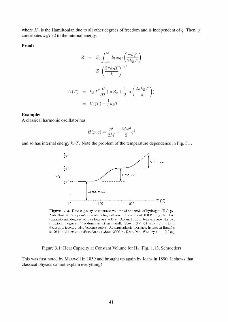
and so has internal energy kBT . Note the problem of the temperature dependence in Fig. 3.1.
Figure 3.1: Heat Capacity at Constant Volume for H2 (Fig. 1.13, Schroeder)
This was first noted by Maxwell in 1859 and brought up again by Jeans in 1890. It shows thatclassical physics cannot explain everything!
41

3.7 Maxwell Speed Distribution
Ref: Schroeder, sect. 6.4.
The probability of a gas particle having momentum px in the x-direction is proportional to
exp
(
− 1
2MkBTp2
x
)
= exp
(
− M
2kBTv2
x
)
By normalising we find
P (vx) =
(
M
2πkBT
)1/2
exp
(
− M
2kBTv2
x
)
so that∫ ∞
−∞
P (vx)dvx = 1
In spherical polar co-ordinatesdvxdvydvz = v2d2Ωvdv
where v =speed = (v2x + v2
y + v2z)
1/2
Normalisation requires∫ ∞
0
dvP (v) = 1
The probability density for finding a particle with speed, v, is
P (v) = 4π
(
M
2πkBT
)3/2
v2 exp
(
− Mv2
2kBT
)
v
P(v
)
vmax
vrms
vmean
Figure 3.2: The Maxwell speed distribution
42
Some typical speeds (‘rms’ is “root mean square”):
Most likely speed: Set dP
dv= 0 ⇒ vmax =
√
2kBT
M
Mean speed =
∫ ∞
0
dv vP (v) ⇒ v =
√
8kBT
πM
Mean square speed = v2 =
∫ ∞
0
dv v2P (v) ⇒ vrms =
√
3kBT
M
3.8 Maxwell’s Demon
References:
H. C. von Baeyer, Warmth disperses and time passes: a history of heat
H. S. Leff and A. F. Rex, Maxwell’s demon: entropy, information, and computing (Adam Hilger,Bristol, 1990).
Feynman lectures on physics, vol. 1, ch. 46.
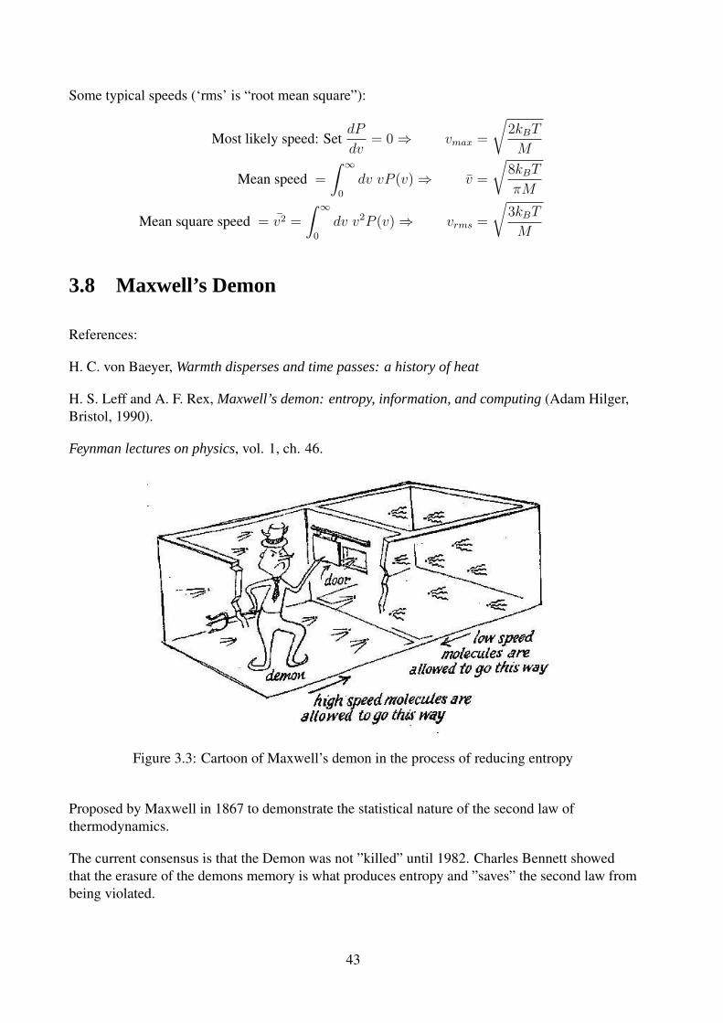
Figure 3.3: Cartoon of Maxwell’s demon in the process of reducing entropy
Proposed by Maxwell in 1867 to demonstrate the statistical nature of the second law ofthermodynamics.
The current consensus is that the Demon was not ”killed” until 1982. Charles Bennett showedthat the erasure of the demons memory is what produces entropy and ”saves” the second law frombeing violated.
43

3.9 Gibbs Paradox
Let’s calculate the entropy of a classical gas
S = −(
∂F
∂T
)
V
=∂
∂T(kBT ln Z)
= kB ln Z + kBT · 3
2· N · 1
T
S
kB
= N
(
3
2+ ln
[
V
(
2πMkBT
h2
)3/2])
Difficulties:
1. S is not extensive If V → 2V and N → 2N , then we want S → 2S, but it does not.
2. S(T ) violates the third law of thermodynamics since as T → 0, S(T ) → −∞
3. Gibbs Paradox
Take the system and insert a partition in the middle.
∆S = Sf − Si
=
(
2
(
N
2ln
(
V
2
))
− N ln V
)
kB
= −NkB ln 2
Hence we have decreased the entropy and violated the second law of thermodynamics!
3.10 Resolution of the Gibbs Paradox
The above derivation of Z(V, T ) for an ideal gas neglected the fact that the particles areindistinguishable. We should write
ZN =1
N !zN
As a result
F −→ Fold + kBT ln N !
S −→ Sold − kB ln N !
' Sold − kB(N ln N − N)
44

where we have used Stirling’s approximation. We have now derived the Sackur-Tetrode equation(for the entropy of a classical gas).
S = NkB
(
5
2+ ln
[
V
N
(
2πMkBT
h2
)3/2])
Note:
1. This is extensive, so that if we make the replacements N → 2N , V → 2V then this resultsin S → 2S. If we partition the system the entropy does not change
2. There is still the problem that the entropy becomes negative at low temperatures - seetutorial problem.
3. Prior to its theoretical derivation the Sackur-Tetrode equation was derived empirically fromexperimental data.
3.11 Creating Entropy
For the ideal gas
S = NkB
(
5
2+ ln
(
V
N
)
+3
2ln T + const.
)
In general we can increase S by increasing N , V or T . If we fix N and V and heat the system theentropy increases. However heat is not necessary to increase entropy. Consider the following caseof free expansion of a gas into a vacuum (see Figure 3.4).
gas "vacuum"inital state
adiabatic enclosure
Figure 3.4: Free expansion of gas into a vacuum
• Remove the partition
• No heat flows into or out of the gas, ⇒ Q = 0
• The gas does not push against anything when it expands, ⇒ W = 0
• Therefore ∆U = Q + W = 0
• But the entropy of the gas increases. Thus heat is not necessary for an entropy increase.
45

3.12 Quantum Statistical Mechanics
exp(−F/kBT ) = Z =∑
i
exp(−Ei/kBT )
where Ei are the quantum energy levels of the system.
3.13 Quantum Ideal Gas
Consider a particle of mass, M , in a cube of dimensions L × L × L. Schrodinger’s equation is:
−~2
2M
(
∂2
∂x2+
∂2
∂y2+
∂2
∂z2
)
Ψ(x, y, z) = EΨ(x, y, z)
The boundary conditions are
Ψ(0, y, z) = Ψ(L, y, z) = 0
Ψ(x, 0, z) = Ψ(x, L, z) = 0
Ψ(x, y, 0) = Ψ(x, y, L) = 0
The solution isΨ(x, y, z) = A sin
(nxπx
L
)
sin(nyπy
L
)
sin(nzπz
L
)
Where A is a normalisation constant, and nx, ny, nz are positive integers → quantum numbers.
E = ε(nx, ny, nz) =~
2
2M
(π
L
)2
(n2x + n2
y + n2z)
The partition function for a single particle is
z =∞∑
nx=1
∞∑
ny=1
∞∑
nz=1
exp (−ε(nx, ny, nz)/kBT )
The spacing of the energy levels is
∼ ~2
2M
(π
L
)2
kBT.
For sufficiently large systems we can take the continuum limit (i.e., treat the n’s as continuousvariables,
z =
∫ ∞
0
dnx
∫ ∞
0
dny
∫ ∞
0
dnz exp (−α(n2x + n2
y + n2z))
whereα ≡ (π~)2
2ML2kBT
We may write this asz = z3
46

where
z =
∫ ∞
0
dn exp (−αn2)
=1
2
√
π
α
(c.f. derivation of the partition function for a classical ideal gas)
z = nQV
V ≡ L3, and
nQ ≡(
MkBT
2π~2
)3/2
≡ 1
λ3T
Since, using the de Broglie relation, p = h/λ
〈KE〉 ∼ kBT =p2
2M
=h2
2Mλ2T
⇒ λ ∼√
h2
MkBT
λT is called the (thermal) de Broglie wavelength of a particle with energy kBT
3.14 Identical Particles
Consider a system with two particles, each of which occupies a separate energy level. Up untilnow, if we interchange the two particles then this leads to two different terms in the partitionfunction. This is correct as long as the particles are distinguishable: e.g. a helium atom and aneon atom.
However, if the particles are identical they should only be counted once. If there are distinctsingle particle states
ZN1 =
(
∑
i
e−βεi
)N
then each entry occurs N ! times. This is overcounting! We should write
ZN =1
N !ZN
1
Note:We are implicitly assuming that there are many more energy levels than particles, i.e. we are notconsidering the possibility of more than one particle in a level. Later, we will relax thisassumption when we consider fermions and bosons.
47

3.15 Quantum Ideal Gas — continued
ZN =1
N !(nQV )N
P = kBT∂
∂Vln ZN
=NkBT
V
To calculate the entropy
S = −(
∂F
∂T
)
=∂
∂T(kBT ln Z)
= kB ln Z + kBT∂
∂Tln ZN
now using ZN = (nQV )N/N ! and Stirling’s approximation
ln ZN = N ln (nQV ) − ln N !
∂
∂Tln ZN = N
∂
∂Tln nQ =
3
2
N
T
Putting this into the above formula for the entropy, we again have the Sackur-Tetrode equation
S = NkB
(
5
2+ ln
(
nQV
N
))
Comparing the classical and quantum expressions we now see that they agree if the h in theclassical expression is Planck’s constant!
48

Chapter 4
Paramagnetism
Key Concepts
• Magnetisation of magnetic materials
• Two state paramagnet
– microcanonical treatment– canonical treatment
• 2J + 1 state paramagnet
• Brillouin function
• Cooling by adiabatic demagnetisation
Reading
D.V. Schroeder, Section 3.3 and p.145-146
M.W. Zemansky, Heat and Thermodynamics, Fifth edition (McGraw Hill, 1968), p.446-455
Ashcroft and Mermin, Solid State Physics, Ch. 31
Demonstrations
19-22 Paramagnetism and Diamagnetism
19-23 Dysprosium in Liquid Nitrogen
49

4.1 Magnetisation
Electrons have a magnetic moment m due to their spin and due to their orbital angularmomentum.
For a system of N electrons or ions the magnetisation is defined as
M =
⟨
N∑
i=1
mi
⟩
where 〈a〉 denotes a thermal average.
4.1.1 Magnetic Materials
1. Paramagnets: M = χB where χ > 0i.e. the moments are parallel to an external magnetic field B
Examples: electrons in a metal, ions in an insulator where the electron shell is partially full.
2. Diamagnets: M = χB where χ < 0i.e. m and B are anti-parallel.Examples: ions with full electronic shells in an insulator, superconductors.
3. Ferromagnet: M 6= 0 when B = 0, for T < Tc
↑↑↑↑↑↑Moments form domains, all aligned in the same direction below the critical temperature Tc
(also known as the Curie temperature). Above Tc there is no spontaneous magnetisation.Examples: Fe, Co, Ni.
4. Antiferromagnets M = 0 but 〈mi〉 6= 0 for B = 0↑↓↑↓↑↓Adjacent moments are anti-aligned, leading to no overall magnetisation.Examples: MnO, FeO.
4.2 Non-interacting two-state paramagnet
Consider a system of N spin-half particles (e.g. electrons) that are localised in the presence of aconstant magnetic field B, pointing in the z-direction. Because they are localised the particles arefixed in position and are hence distinguishable.
The effect of the field is to tend to align the magnetic dipole moment m of each particle parallelto the field.
50

The Hamiltonian for a single moment is
H = −m · B= −mzBz
= −mB
since we take B to point in the z-direction. The energy is lower when the magnetic moment isparallel to the magnetic field (−mB as opposed to mB).
For spin-half particles, mz can have eigenvalues ±µ so the allowed energy levels are
E = ±µB
For electrons,m = −g0µBS
where S is the spin operator, and g0 is the g-factor or gyromagnetic ratio. Its value has beencalculated very precisely in QED, and is g0 = 2.002319. The Bohr magneton µB is given by
µB ≡ eh
4πme
,
= 9.27 × 10⁻²⁴J/T,
= 5.79 × 10⁻⁵eV/T.
The total energy of the system is
U = µB(N↓ − N↑) = µB(N − 2N↑) (4.1)
where N = N↑ + N↓, N↑ is the number of particles with spin up, and µ = g0µB/2. Themagnetisation M is the total magnetic moment of the whole system
M = µ(N↑ − N↓) = −U
B. (4.2)
4.2.1 Microcanonical Ensemble
We now find M as a function of B and the temperature T using the microcanonical ensemble.
The multiplicity of the system isΩ(U,N) =
N !
N↑!N↓!
as stated in Section 2.3. The entropy is
S(U,N)
kB
= N ln N − N↑ ln N↑ − (N − N↑) ln(N − N↑) (4.3)
51

where we have used Stirling’s approximation. The temperature is given by
1
T=
(
∂S
∂U
)
N,B
=∂N↑
∂U
∂S
∂N↑
= − 1
2µB
(
∂S
∂N↑
)
. (4.4)
Now using (4.3) gives
1
kB
(
∂S
∂N↑
)
N
= − ln N↑ − 1 + ln(N − N↑) + 1
= ln
(
N − N↑
N↑
)
= ln
(
N↓
N↑
)
(4.5)
So that from Equations 4.4 and 4.5
N↓
N↑
= exp
(
−2µB
kBT
)
.
To find the mean magnetic moment M/N , we use Equation 4.2 and N = N↑ + N↓,
M
N=
µ(N↑ − N↓)
N↑ + N↓
,
=µ(1 − N↓/N↑)
1 + N↓/N↑
,
= µ
[
1 − exp (−2µB/kBT )
1 + exp (−2µB/kBT )
]
.
Hence,M = µN tanh
(
µB
kBT
)
. (4.6)
As you should be coming familiar with in this course, the first thing that we do is check the highand low temperature limits.
High temperature / low field: We have µB kBT . Since tanh x ' x for x 1 then,
M
NB=
µ2
kBT
which is Curie’s law that we came across in the tutorials.
Notice as T → ∞, M → 0, because the electrons are so energetic that the difference between theenergies of the spin up and spin down states becomes negligible, and their spins are randomlyaligned.
52

Low temperature / high field: We have µB kBT . In this case
M = µN
i.e. all the moments are parallel to the field.
The internal energy (again from Equation 4.2) is given by
U(T ) = −MB,
= −NµB tanh
(
µB
kBT
)
. (4.7)
Heat capacity in a constant field is
CB(T ) =
(
∂U
∂T
)
N,B
= NkB(µB/kBT )2
cosh2(µB/kBT )(4.8)
These are shown in Figure 4.1. The peak in the CB(T ) versus T curve is known as the Schottkyanomaly, as we have seen already in tutorials.
4.2.2 Canonical ensemble
We now recalculate our result using the canonical ensemble. This calculation will give you anidea about why it is much preferred to the microcanonical!
The partition functionZ(B, T ) = z(B, T )N
where z is the partition function for a single magnetic moment. Note here that we don’t have todivide by N ! as we did for the ideal gas — this is because the magnetic moments aredistinguishable.
The partition function for a single moment is particularly simple, as there are only two possibleenergy states. We have looked at such a system already in tutorials.
z(B, T ) =∑
s
e−βEs ,
= e−βµB + eβµB,
= 2 cosh
(
µB
kBT
)
.
53

−6 −4 −2 0 2 4 6
−1
−0.5
0
0.5
1
kB T / µ B
M /
µ N
Magnetisation for a two state paramagnet
0 1 2 3 4 5 60
0.1
0.2
0.3
0.4
0.5
kB T / µ B
CB /
k B N
Heat capacity for a two state paramagnet
Figure 4.1: Magnetisation and heat capacity for a two-state paramagnet. Note that you can getnegative temperatures for this system. See Appendix E, Kittel and Kroemer for further details.This is also mentioned in Schroeder, pg 101-2.
54
The internal energy is
U(T ) = kBT 2
(
∂ ln Z
∂T
)
B
,
= NkBT 2 ∂
∂Tln
[
cosh
(
µB
kBT
)]
,
= −NkBT 2 · µB
kBT 2
sinh (µB/kBT )
cosh (µB/kBT ),
= −NµB tanh
(
µB
kBT
)
.
This agrees with the microcanonical ensemble. Notice that this is a lot quicker and easier than themicrocanonical formulation.
4.3 Insulators of Ions with Partially Full Shells
In solids containing ions such as Fe3+, Fe2+, Cr2+ and Mn4+, the electrons in the outermostatomic orbitals (usually d-orbitals) have spin S and orbital angular momentum L.
The state is completely specified by L,S, the total angular momentum vector J = L + S and themagnetic quantum number MJ which can take 2J + 1 possible values in the range of−J,−J + 1, . . . , J − 1, J . (This is very similar to the azimuthal angular momentum m in ahydrogen atom, only now we consider the total angular momentum.)
Hund’s rules are used to determine the basic electron configuration of an atom or ion. These aredescribed in detail in Chapter 31 of Ashcroft and Mermin, however if you prefer the internet tothe library you can find them athttp://hyperphysics.phy-astr.gsu.edu/hbase/atomic/hund.html
In brief, Hund’s rules say that for the ground state, the electrons in the outer shell will arrangethemselves to have
1. The maximum value of the total spin S allowed by the exclusion principle.
2. The maximum value of the total angular momentum L consistent with this value of S.
3. The value of the total angular momentum J is equal to |L − S| when the shell is less thanhalf full, and to L + S when the shell is more than half full. When the shell is half full thefirst rule gives L = 0 so J = S.
The first rule has its origin in the exclusion principle and the Coulomb repulsion between twoelectrons. The second — is best accepted from model calculations! The third is a consequence ofthe spin-orbit interaction — for a single electron the energy is lowest when the spin isanti-parallel to the orbital angular momentum.
55

It can be shown that in a magnetic field B = Bz that the magnetic moment of an ion withquantum numbers J, L, S,MJ is
m = −g(JLS)µBMJ
and that the allowed energies are (similar to the spin-half case)
E(MJ) = −mB
= g(JLS)µBMJB (4.9)
where the Lande g-factor of the ion is
g(JLS) =1
2(g0 + 1) − 1
2(g0 − 1)
L(L + 1) − S(S + 1)
J(J + 1)
g0 = 2.002319 is the electron g-factor.
Example
For Fe3+, one can calculate that L = 0 and S = 52, related to the fact that Hund’s rule says that
each electron should be placed in a separate state with parallel spins, and Fe3+ has 5 electrons inits outer orbital, each with spin- 1
2. Hence J = 5
2, and g = g0 since J = S.
4.3.1 Partition function
In the same manner as for the two state paramagnet
Z(B) =∑
s
e−βEs
= z(B)N
where z(B) is the partition function for a single magnetic moment and we assume they do notinteract. To save ourselves some writing, we define
a =gµBB
kBT.
There are 2J + 1 different energy levels so
z(B) =
MJ=J∑
MJ=−J
exp(−aMJ),
= e−aJ + e−a(J−1) + · · · + ea(J−1) + eaJ ,
= e−aJ(
1 + ea + e2a + · · · + e2aJ)
.
We now use the fact thatN−1∑
n=0
xn =1 − xN
1 − x.
56

We write the partition function sum as
z(B) = e−aJ
2J∑
n=0
(ea)n ,
= e−aJ 1 − e(2J+1)a
1 − ea,
=e−aJ − e(J+1)a
ea/2 (e−a/2 − ea/2),
=sinh((J + 1/2)a)
sinh(a/2).
4.3.2 Magnetisation
If the magnetic field is in the z-direction, the magnetic moment in the state |JMJ〉 is −gµBMJ asstated at the start of this section.
The fractional magnetisation in thermal equilibrium is
M
N=
∑
MJ
(−gµBMJ)1
ze−βE(MJ )
= −gµB
∑
MJ
MJ
zexp
(
−gµBMJB
kBT
)
= kBT1
z
(
∂z
∂B
)
T
M = kBTN∂
∂B(ln z)
= kBTN∂a
∂B
∂
∂a
[
ln sinh
(
(J +1
2)a
)
− ln sinh(a
2)
]
and thusM = NgµB
[
(J +1
2) coth
(
(J +1
2)a
)
− 1
2coth(
a
2)
]
(4.10)
We can writeM = NgµBJBJ(a) (4.11)
whereBJ(a) =
1
J
[
(J +1
2) coth
(
(J +1
2)a
)
− 1
2coth(
a
2)
]
(4.12)
is known as the Brillouin function. Although not immediately obvious, for J = 12
and g = g0 itreduces to the spin-half result. As always, let’s check the limits:
Low temperature / high field:
a =gµBB
kBT 1, coth
(a
2
)
→ 1, coth
(
(J +1
2)a
)
→ 1
57

and so we haveM → NgµBJ
i.e. all the magnetic moments are aligned parallel to the field as expected.
High temperature / low field
a 1, and for small x 1,coth x =
1
x+
x
3+ . . .
This means
M
NgµB
≈ (J +1
2)
(
1
(J + 12)a
+1
3(J +
1
2)a
)
− 1
2
(
2
a+
a
6
)
=1
a− 1
a+
a
3
(
(J +1
2)2 − 1
4
)
=1
3J(J + 1)a
SoM = N(gµB)2J(J + 1)B
3kBT(4.13)
which is Curie’s law again.
The Brillouin function can be tested experimentally on crystals such asFe2(SO4)3·(NH4)2 SO4 · 24H2O
which have crystal structures such that the magnetic ions (in this case Fe3+) are very isolatedfrom one another and so the magnetic dipoles interact very weakly with one another. Acomparison between experimental results and the Brillouin function is shown in Fig. 4.2.
4.3.3 Internal Energy and Entropy
U(T ) = −MB
We also haveU(T ) = kBT 2 ∂
∂Tln Z(B, T )
As before, we can showF ≡ U − TS = −kBT ln Z(B, T )
Thus,S = −
(
∂F
∂T
)
B
58

Figure 4.2: Plot of magentic moment versus B/T for spherical samples of (I) potassium chromiumalum, (II) ferric ammonium alum, and (III) gadolinium sulfate octahudrate. Over 99.5% mageneticsaturation is achieved at 1.3K and about 5T. The points are experimental results of W.E. Henry(1952) and the solid curves are graphs of the Brillouin function. [Taken from Introduction to SolidState Physics, C. Kittel, 6th ed. 1 kG = 103 G, 104 G = 1 T.]
59
and soS
kB
= ln Z(B, T ) + T∂
∂Tln Z(B, T )
= ln Z +U
kBT
= ln Z − MB
kBT
= ln Z(a) − B∂
∂Bln Z(a)
= ln Z(a) − a∂
∂aln Z(a)
So the entropy is an increasing function with a:
S(B, T ) = kBf
(
gµBB
kBT
)
. (4.14)
i.e., the entropy is only a function of the ratio B/T . Hence, in an adiabatic process (S is fixed)and if B decreases then T must decrease too.
z(a) =sinh[(J + 1/2)a]
sinh(a/2)
S
kB
= ln (sinh[(J + 1/2)a]) − (J + 1/2)a coth[(J + 1/2)a)]
− ln[sinh(a/2)] +a
2coth(a/2) (4.15)
As a → 0 (T → ∞):z(a) → 2J + 1, S → kB ln(2J + 1).
As a → ∞ (T → 0):z(a) → eJa, S → kB(Ja − aJ) = 0.
4.3.4 Cooling by adiabatic demagnetisation
The paramagnetic crystal to be cooled begins in thermal equilibrium with e.g. liquid helium.
1. The system is held at constant temperature T = Ti. The magnetic field is increased to afield value Bi.
2. The system is adiabatically isolated.
3. The field is slowly reduced to Bf .
The entropy S(B/T ) must remain constant in step 3. Hence, the final temperature is
Tf = TiBf
Bi
< Ti
60
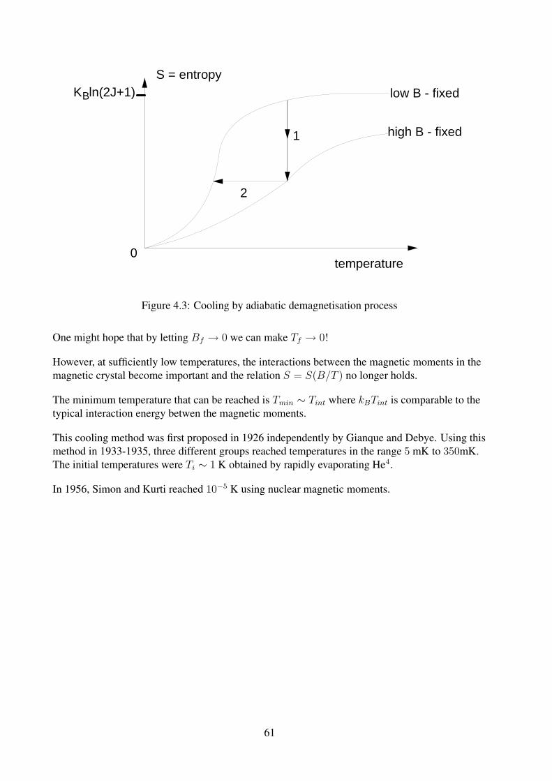
1
2
low B - fixed
temperature
S = entropyK ln(2J+1)B
0
high B - fixed
Figure 4.3: Cooling by adiabatic demagnetisation process
One might hope that by letting Bf → 0 we can make Tf → 0!
However, at sufficiently low temperatures, the interactions between the magnetic moments in themagnetic crystal become important and the relation S = S(B/T ) no longer holds.
The minimum temperature that can be reached is Tmin ∼ Tint where kBTint is comparable to thetypical interaction energy betwen the magnetic moments.
This cooling method was first proposed in 1926 independently by Gianque and Debye. Using thismethod in 1933-1935, three different groups reached temperatures in the range 5 mK to 350mK.The initial temperatures were Ti ∼ 1 K obtained by rapidly evaporating He4.
In 1956, Simon and Kurti reached 10−5 K using nuclear magnetic moments.
61

62

Chapter 5
Thermal Radiation
Key concepts
• The ultraviolet catastrophe
• The Planck distribution
• Summing over modes
• The Planck spectrum
• Blackbody radiation
• Cosmic background radiation
Reading
Schroeder, Section 7.4Kittel & Kroemer, Ch 4
Demonstrations
Video encyclopedia of physics demonstrations, DVD edition (Education Group, 2000). [PSElibrary QC33.V53 2000]
24-18: Radiation spectrum of a hot object
63

5.1 Ultraviolet catastrophe
Consider classical electromagnetic waves confined to a box of fixed volume, V = L3. There arean infinite number of modes of vibration for the electromagnetic waves, with wavelengths
λn =2L
nn = 1, 2, 3, . . .
By considering the total energy of the electromagnetic field, we can show that each mode behaveslike a classical harmonic oscillator. Thus, by the equipartition theorem each mode must have anaverage energy of kBT (as there are two degrees of freedom). As there are an infinite number ofmodes, then the total electromagnetic energy in the box must also be infinite.
n=1
n=2
n=3
0 L
Figure 5.1: Modes of a electromagnetic radiation within a box of width L
However, when we open the oven door we don’t get blasted with an infinite amount of energy, sosomething must be wrong with this model. This is called the ultra-violet catastrophe. Why?
This represents a failure of classical statistical mechanics.
5.2 The Planck distribution
The solution to the ultraviolet catastrophe led to the birth of quantum mechanics (Planck, 1900).Suppose that an oscillator with frequency ν can only have discrete energies
En = nhν, n = 0, 1, 2, . . .
where h is Planck’s constant. This is ignoring the zero point energy. The partition function for thesingle oscillator is
Z =∞∑
n=0
exp(−nhν/kBT ) =1
1 − exp(−hν/kBT ).
64

The average energy is
U = kBT 2 1
Z
∂Z
∂T
=hν
exp(hν/kBT ) − 1
The average number of quanta of energy hν is then the total energy divided by hν
n(ν) =U
hν=
1
exp(hν/kBT ) − 1
This is the Planck distribution.
For high frequency modes, hν kBT , n(ν) ' exp(−hν/kBT ) 1. These modes are “frozenout” and don’t contribute to the total energy of the system.
5.3 Summing over modes
We now find the total energy in the box using the Planck distribution. In one dimension theallowed wavelengths are
λn =2L
nn = 1, 2, 3, . . .
The momenta of these wavelengths are
pn =h
λn
=h
2Ln,
and the energy of each mode is
εn = pnc =hc
2Ln.
In three dimensions we have
ε = |p| c = c[
p2x + p2
y + p2z
]1/2, (5.1)
where px, py, pz are the x, y, and z components of the momentum, and are given by
px =h
2Lnx, py =
h
2Lny, pz =
h
2Lnx, nx, ny, nz = 1, 2, 3, . . .
with
εn =hc
2L|n| n = (nx, ny, nz)
Each mode (photon) can have two possible polarisations. The total energy is then
U = 2∑
n
εnn(εn),
=∑
n
hc
L|n|[
1
exp(|n|hc/2LkBT ) − 1
]
65

Wavelength λ
Ene
rgy
dens
ity u
(hc/
λ)
Rayleigh−Jeans law(classical)
Planck distribution
UV catastrophe
Figure 5.2: The Planck distribution compared with the classical Rayleigh-Jeans law (as a functionof wavelength, not energy!) Classical physics can account for the long-wavelength, low energymodes where there are many photons per mode. However, it predicts a UV catastrophe for shortwavelengths.
For large L we can convert the sum to an integral
∑
n
→ 1
8× 4π
∫ ∞
0
n2dn,
where we multiply by one eighth because all the ni must be positive, and so we only want oneoctant of the 3D space. This gives
U =hcπ
2L
∫ ∞
0
n3dn
exp(hcn/2LkBT ) − 1, (5.2)
If we make a change of variables to ε = hcn/2L then we find the total energy density is
U
L3=
∫ ∞
0
8π
(hc)3
ε3dε
exp(ε/kBT ) − 1,
=
∫ ∞
0
u(ε)dε,
whereu(ε) ≡ 8π
(hc)3
ε3
exp(ε/kBT ) − 1, (5.3)
is the spectrum or energy density per unit photon energy, which is plotted in Fig. 5.2. It has amaximum at ε = 2.82kBT (Wien’s law).
For ε kBT , u(ε) ∼ ε2kBT , as expected classically.
66

For ε kBT , u(ε) ∼ ε3 exp(−ε/kBT ) ε2kBT , and so the energy density of high energyradiation is suppressed, preventing the ultra-violet catastrophe.
By making another change of variables x = ε/kBT , we can change the expression (5.3) into theform
U
V=
8π (kBT )4
(hc)3
∫ ∞
0
x3dx
ex − 1. (5.4)
The integral in Eqn. (5.4) evaluates to π4/15 (see the Appendix of Schroeder). Note thatU/V ∼ T 4. Hence, doubling T increases U/V by a factor of 16.
Also the heat capacity CV (T ) = (∂U/∂T )V ∼ T 3, approaches zero as the temperature goes tozero, which is consistent with the third law of thermodynamics.
5.4 Blackbody radiation
Blackbody radiation comprises the photons emitted by any non-reflecting (“black”, i.e. perfectlyabsorbing) surface at a fixed temperature T . A blackbody emits the same photon spectrum asdoes a hole in a box at the same temperature.
TT
black body
Box of photons
Figure 5.3: A hollow box and a blackbody in thermal equilibrium.
We can see this by considering a blackbody and a hole in a box with equal area in thermalequilibrium. If the blackbody does not emit the same spectrum as the box, then there will be a netflow of energy from the one emitting more energy to the one emitting less energy. But since thetwo are in thermal equilibrium, there can be no net energy flow between the two objects.
This does not mean that the spectrums are the same — you could imagine a situation where thespectrum of each object was different, but there was no net energy flow. However, the argumentcan be extended as we can always insert a filter between the box and the blackbody that blocks acertain frequency range.
Imagine the two spectrums are not the same. This means that the energy being emitted for somefrequency range will be different for the two objectw. If we place a filter between the two objects
67

that blocks this range, it means that there will then be a net flow of energy, which violates ourassumption of thermal equilibrium.
We can arbitrarily choose any filter, with any frequency range, which means that the radiationemitted by a blackbody must have the same spectrum as a box at the same temperature.
The power per unit area emitted by the hole, and so also the blackbody, is
P
A=
c
4
U
V
The factor of 1/4 comes from a somewhat involved geometric calculation that works out the totalenergy that escapes from the box in a time interval dt (see Schroeder, pg 300–2). SubstitutingEqn. (5.4) into the formula for the power per unit area results in Stefan’s law
P
A= σT 4, σ =
2π5k4B
15h3c2.
The Stefan-Boltzmann constant is σ = 5.67 × 10⁻⁸ W m−2 K2. Stefan’s law was discoveredempirically in 1879.
5.5 Cosmic background radiation
Cosmic background radiation was predicted in the late 1940’s by Alpher, Hermann and Gamowas being a remnant of the “big bang”. The cosmic background radiation are the photons whichwere last scattered off electrons 300,000 years after the beginning of the universe, when thetemperature was approximately 3000 K. In the meantime the universe has expanded by about afactor of 103 in every direction, and this has caused the wavelengths of this radition to bestretched — red-shifted, if you like. It was first observed accidentally in 1964 by Penzias andWilson, who originally thought it was noise due to pigeon droppings in their radio telescope. Forthis discovery they received the Nobel prize in 1978.
The cosmic background radiation is incredibly uniform and isotropic. In 1989, the CosmicBackground Explorer (COBE), a NASA satellite, found that the cosmic background radiation hasthe spectrum of a blackbody with a temperature T = 2.728 ± 0.002K and the deviation from thePlanck spectrum is less than 0.005%. In 1992 using the differential microwave radiometer onCOBE temperature fluctuations of 30 µK on an angular scale of 10 degrees was found. This wasimportant because it provided evidence for spatially inhomogeneous regions needed in the earlyuniverse to form galaxies.
Very recent results from the Wilkison Microwave Anisotropy Probe (WMAP) satellite have madea far more accurate measurement of the temperature fluctuations (see Fig. 5.5, 5.6), and these areare consistent with the inflationary model of the early universe. The most precise calculation ofthe age of the universe was made using data from this satellite in 2003 — it gives an age of13.7 ± 0.2 billion years.
A summary of findings from the WMAP measurements (from the WMAP website):
68

• Universe is 13.7 billion years old, with a margin of error of close to 1%.
• First stars ignited 200 million years after the Big Bang.
• Light in WMAP picture is from 379,000 years after the Big Bang.
• Content of the Universe:
– 4% Atoms, 23% Cold Dark Matter, 73% Dark Energy.– The data places new constraints on the Dark Energy. It seems more like a
“cosmological constant” than a negative-pressure energy field called “quintessence”.But quintessence is not ruled out.
– Fast moving neutrinos do not play any major role in the evolution of structure in theuniverse. They would have prevented the early clumping of gas in the universe,delaying the emergence of the first stars, in conflict with the new WMAP data.
• Expansion rate (Hubble constant) value: Ho = 71 (km/sec)/Mpc (with a margin of error ofabout 5%)
• New evidence for Inflation (in polarized signal)
• For the theory that fits our data, the Universe will expand forever. (The nature of the darkenergy is still a mystery. If it changes with time, or if other unknown and unexpected thingshappen in the universe, this conclusion could change.)
Further reading
http://map.gsfc.nasa.gov/C. L. Bennett et al., Physics Today, November, 1997, p.32.M. Roos, Introduction to Cosmology, (Wiley, Chichester, 1997), Second edition, Chapter 5.
69

Figure 5.4: Spectrum of the cosmic background radiation, as measured by the COBE satellite.The vertical axis is the energy density. Note that a frequency of f = 3 × 10¹¹ s−1 correspondsto a wavelength λ = 1.0 mm. The point by point uncertainties are too small to show up onthis scale; the size of the squares estimates systematic uncertainties. The best fit temperature is2.728 ± 0.002 K. Graph taken from Schroeder.
70
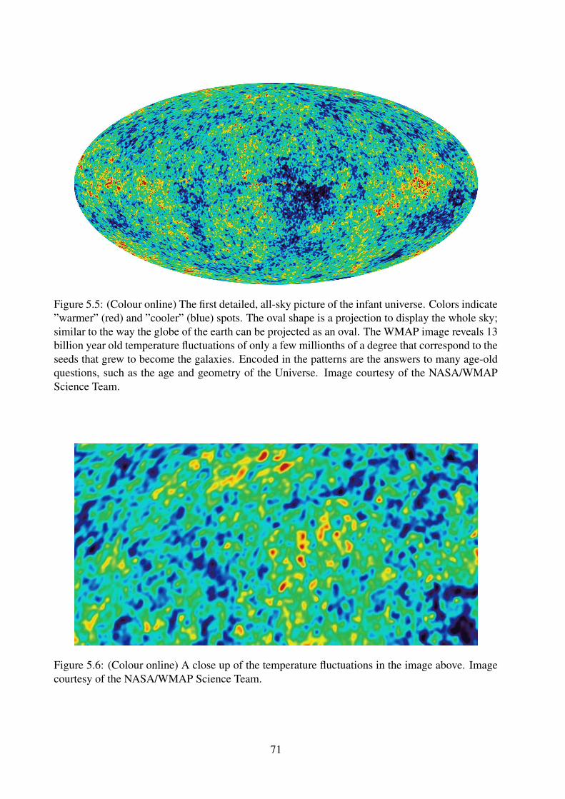
Figure 5.5: (Colour online) The first detailed, all-sky picture of the infant universe. Colors indicate”warmer” (red) and ”cooler” (blue) spots. The oval shape is a projection to display the whole sky;similar to the way the globe of the earth can be projected as an oval. The WMAP image reveals 13billion year old temperature fluctuations of only a few millionths of a degree that correspond to theseeds that grew to become the galaxies. Encoded in the patterns are the answers to many age-oldquestions, such as the age and geometry of the Universe. Image courtesy of the NASA/WMAPScience Team.
Figure 5.6: (Colour online) A close up of the temperature fluctuations in the image above. Imagecourtesy of the NASA/WMAP Science Team.
71