COMMON LOON (GAVIA IMMER) BIOGEOGRAPHY AND REPRODUCTIVE

SUCCESS IN AN ERA OF CLIMATE CHANGE

By

Allison Byrd

B.A. University of Rhode Island, 2001

A THESIS

Submitted in Partial Fulfillment of the

Requirements for the Degree of

Master of Science

(in Ecology and Environmental Science)

The Graduate School

The University of Maine

May, 2013

Advisory Committee:

Brian Olsen, Assistant Professor of Biology & Ecology, Advisor

Rebecca Holberton, Professor of Biology

David Evers, Executive Director, Biodiversity Research Institute

ii

THESIS ACCEPTANCE STATEMENT

On behalf of the Graduate Committee for Allison Byrd I affirm that this

manuscript is the final and accepted thesis. Signatures of all committee members are on

file with the Graduate School at the University of Maine, 42 Stodder Hall, Orono, Maine.

Brian Olsen, Assistant Professor of Biology & Ecology December 3, 2012

LIBRARY RIGHTS STATEMENT

In presenting this thesis in partial fulfillment of the requirements for an advanced

degree at The University of Maine, I agree that the Library shall make it freely available

for inspection. I further agree that permission for “fair use” copying of this thesis for

scholarly purposes may be granted by the Librarian. It is understood that any copying or

publication of this thesis for financial gain shall not be allowed without my written

permission.

Signature:

Date:

COMMON LOON (GAVIA IMMER) BIOGEOGRAPHY AND REPRODUCTIVE

SUCCESS IN AN ERA OF CLIMATE CHANGE

By: Allison Jeanne Byrd

Thesis Advisor: Dr. Brian J. Olsen

An Abstract of the Thesis Presented

in Partial Fulfillment of the Requirements for the

Degree of Master of Science

(in Ecology and Environmental Science)

May, 2012

Climate change has the potential to shift and restrict ranges for a suite of species.

The birds of the boreal ecosystem, like the Common Loon (Gavia immer), may be

particularly at risk given the changes predicted for this biome. Current range models for

this iconic water bird predict that large sections of the United States may lose the loon in

the next 100 years, but these models are based on habitat correlations and not the

demographic mechanisms that will actually produce the change. The primary goal of our

research was to understand the factors that determine loon vulnerability to climatic

change at multiple scales. We applied a recursive partitioning technique to analyze loon

presence/absence in 288 lakes across the southern edge of their North American

distribution using 112 abiotic and landscape-level factors. The resulting binary tree

(“decision tree”) classified lakes into groups based on the probability of loon presence,

while maximizing homogeneity within the resultant two nodes. The most significant

splits in the cross-validated tree were created using using lake salinity, acidity, and

sulfate levels. We employed similar methods to compare loon occupancy and seasonal

fecundity at a smaller scale (New England) to elucidate potential demographic

mechanisms of loon persistence. Results from twenty potential predictors suggest that

similar processes are driving loon presence/absence both continentally and within New

England (lake salinity, alkalinity, and lake surface area). Loon productivity, on the other

hand, was best predicted using the size of the lake and its drainage basin. Lake surface

area and characteristics of the drainage basin are thus good predictors of both loon

distribution and loon productivity, and are thus also likely to be useful in predicting range

shifts in the future. As few (if any) of the predictors of productivity in the best decision

trees are likely to change dramatically with climate, these outcomes suggest that future

range alteration for loons due to climate change are likely to be more sensitive to annual

adult survival (which will influence breeding ground settlement patterns) than

environmental factors encountered on the breeding grounds.

After highlighting the environmental factors that predict loon occupancy and

productivity, we explored environmental predictors of individual energetic condition.

Physiological measures may offer more information about the likelihood of loon

persistence, because they can identify covariance between energetic condition and

breeding habitat quality. We used blood metabolites and behavioral observations to

evaluate the energetic costs of common loons (Gavia immer) breeding on lakes across a

gradient of environmental, spatial, and social conditions. Using samples collected over

two years (n=97) along the species’ southern breeding range edge (ME, NH, MA, MT,

WA), we identified the number of offspring, daily maximum temperature, and latitude as

the most important drivers of the energetic cost of maintaining a breeding territory.

Specifically we found that: 1) loons with two chicks expend more energy than those with

one, 2) loons near the southern range edge expend more energy to produce a given brood

size than those nearer the range center and, 3) birds breeding in warmer temperatures

expend more energy than those in cooler temperatures (controlling for year, territory

type, and calendar date, free glycerol levels, size-corrected body mass, and longitude).

We suggest that as environmental conditions change in the coming years, blood

metabolites offer a promising predictor of population collapse along range boundaries.

Energetic condition deteriorated toward the southern range edge and in warmer

conditions, controlling for the number of offspring produced, which suggests that loons

may be sensitive to increasing global temperatures. We suggest that as environmental

conditions change in the coming years, blood metabolites offer a promising predictor of

population collapse along range boundaries.

iii

ACKNOWLEDGEMENTS

I would like to thank the numerous individuals who made this thesis possible. I

extend a sincere thank you to my committee members David Evers and Rebecca

Holberton for their support. I would also like to thank William Halteman for his

statistical expertise and encouragement as I made my way through the world of data

analysis. I have countless peers who made project possible including Kate Ruskin, Ellen

Robertson, Dave Grunzel, Evan Adams, Leah Culp, Chris Tonra, Adrienne Leppold,

James Style, Anna Henry, Laura Kennedy, Anya Rose, Matt Jones, and also Kate Taylor,

Carrie Osborne, Carl Anderson, Jeff Fair, Alison Jackson, Ginger and Dan Poleschook,

Kristin Ditzler Strock, and Courtney Wigdahl. I cannot sufficiently thank Maureen

Correll, Daniel McConville, and Jenny McCabe for their friendship and support during

my time at UMaine. I’d like to thank Wren for countless laughs, runs, and canine

support. I would like to thank Sue Anderson and Trish Costello for their administrative

assistance throughout my time at the University of Maine. My family provided

encouragement and love, including Barbara, Ray, Adam Byrd, and Melanie, Dan, Lilly,

and Morgan Kerr. Funding was provided by the School for Biology and Ecology,

Biodiversity Research Institute, the Maine Agriculture and Forestry Experimental

Station, and the Northeast Temperate Network of the National Park Service. Field

assistance was provided by Mike Chickering, Tori Polito, Keith Blanchette, Matt O’Neal,

Ashley Malinowski, Seth Wile, and Misty Libby. I’d like to thank David Bishop for

believing in me and putting me in contact with Brian Olsen, which is how this incredible

journey all began

iv

Finally, I would like to extend the most heartfelt thank you possible to my

advisor, Brian Olsen. Brian, you have showed me what it means to balance brilliance,

encouragement, humor, editing, teaching, motivation, family, exercise, grading,

enthusiasm, sarcasm, a seven-plus member lab, confidence, humility, and constant

learning… all without losing your mind. I cannot adequately express how much I have

learned from you during my time here and I could not be more proud to be counted as

one of your first students. You are an incredible teacher and mentor, and I will be forever

thankful for your guidance. Thank you for always believing in me. I dedicate this thesis

to you.

vi

TABLE OF CONTENTS

ACKNOWLEDGEMENTS ............................................................................................................. 1

LIST OF TABLES ........................................................................................................................... 1

LIST OF FIGURES ......................................................................................................................... 1

Chapter

1. COMMON LOON (GAVIA IMMER) BIOGEOGRAPHY AND REPRODUCTIVE

SUCCESS IN AN ERA OF CLIMATE CHANGE: BACKGROUND

AND CONCLUSIONS ............................................................................................................... 1

1.1. DISTRIBUTION ...................................................................................................... 1

1.2. HABITAT ................................................................................................................. 2

1.3. FEEDING ................................................................................................................. 3

1.4. PHYSICAL CHARACTERISTICS ......................................................................... 3

1.5. BEHAVIOR.............................................................................................................. 4

1.6. BREEDING INFORMATION ................................................................................. 5

1.7. SITE FIDELITY ....................................................................................................... 6

1.8. MANAGEMENT AND CONSERVATION ............................................................ 8

1.9. RANGE EDGES ....................................................................................................... 8

1.10. CLIMATE CHANGE ............................................................................................. 9

1.11. MODELING SPECIES DISTRIBUTION IN RESPONSE TO

CLIMATE CHANGE .......................................................................................... 10

vi

1.12. LAKE METRICS PREVIOUSLY SHOWN TO AFFECT LOON

PRESENCE/ABSENCE AND PRODUCTIVITY .............................................. 11

1.12.1. Lake Depth ........................................................................................... 11

1.12.2. Lake Surface Area ................................................................................ 12

1.12.3. Water Clarity/Turbidity ........................................................................ 13

1.12.4. Surface temperature .............................................................................. 13

1.12.5. pH ......................................................................................................... 14

1.12.6. Conductivity ......................................................................................... 15

1.12.7. Dissolved Organic Carbon (DOC)........................................................ 16

1.13. USING TRIGLYCERIDES AND FREE GLYCEROL TO DETERMINE

ENERGETIC COST ............................................................................................ 17

1.14. SYNOPSIS .......................................................................................................... 25

2. MACHINE LEARNING TECHNIQUES: A TOOL FOR UNDERSTANDING COMMON

LOON (GAVIA IMMER) BIOGEOGRAPHY AND PRODUCTIVITY IN AN ERA OF

CLIMATE CHANGE ............................................................................................................... 29

2.1. ABSTRACT ........................................................................................................... 29

2.2. INTRODUCTION .................................................................................................. 30

2.2.1. Climate Change and Freshwater Communities ...................................... 30

2.2.2. Machine Learning: Using Decision Trees and Random Forests to

Determine Variable Importance ............................................................ 32

2.2.3. General Approach ................................................................................... 34

2.3 METHODS .............................................................................................................. 35

2.3.1. Methods Overview ................................................................................. 35

vi

2.3.2. Continental-scale Range Descriptors ...................................................... 36

2.3.3. Regional-scale Range Descriptors .......................................................... 45

2.3.4. Regional Productivity Descriptors .......................................................... 46

2.4. RESULTS ............................................................................................................... 48

2.4.1. Continental-scale Range Descriptors ...................................................... 48

2.4.2. Regional-scale Range Descriptors .......................................................... 52

2.4.3. Regional Productivity Descriptors .......................................................... 55

2.5. DISCUSSION ......................................................................................................... 58

2.5.1. Continental-scale Range Descriptors ..................................................... 58

2.5.2. Regional-scale Range Descriptors .......................................................... 62

2.5.3. Regional-scale Productivity Descriptors ................................................ 63

2.5.4. Validating Envelope Models with Hierarchical Decision Trees ............ 64

2.5.5. Implications for Climate Change on the Range of the Common Loon .. 66

3. BLOOD METABOLITES AS INDICATORS OF BREEDING HABITAT QUALITY: A

SENSITIVE METHOD TO PREDICT RANGE ALTERATION UNDER CLIMATE

CHANGE? ................................................................................................................................ 68

3.1 ABSTRACT ............................................................................................................ 68

3.2 INTRODUCTION ................................................................................................... 69

3.3 MATERIALS AND METHODS ............................................................................ 73

3.3.1. Study population, field methods, and lab assays .................................... 73

3.3.2. Behavioral Observations ......................................................................... 74

3.3.3. Statistics .................................................................................................. 75

3.4 RESULTS ................................................................................................................ 78

vii

3.4.1. Establishing Baseline Metabolic Measures ............................................ 78

3.4.2. Triglyceride Levels In Breeding Loons .................................................. 79

3.4.3. Behavior ................................................................................................. 82

3.5 DISCUSSION .......................................................................................................... 83

3.6 SUMMARY............................................................................................................. 87

BIBLIOGRAPHY .......................................................................................................................... 89

BIOGRAPHY OF THE AUTHOR .............................................................................................. 101

viii

LIST OF TABLES

Table 1. Descriptive Statistics for Metabolite Values…………………………..…..…18

Table 2. Data Sources………………………………………………………….……......37

Table 3. Variables in National Presense/Absence Analysis……………….…..….…...40

Table 4. Variables in New England Presence/Absence Analysis…………….….…….46

Table 5. Variables in New England Productivity Analysis………………….….....…..48

Table 6. Descriptive Statistics for Triglyceride and Free Glycerol Levels………..….79

Table 7. Triglyceride Probability Models………………………………………..….....81

Table 8. Triglyceride Model-Averaged Parameter Estimates……………………...….82

Table 9. Triglyceride Levels of Loons That Escalated Interactions with Intruders…...83

ix

LIST OF FIGURES

Figure 1. Portion Of A Figure From Jenn-Eiermann and Jenni (1994) ...................................... 20

Figure 2. Figure From Jenni-Eiermann And Jenni (1992) .......................................................... 22

Figure 3. Figure From Jenni and Schwilch (2001) ..................................................................... 24

Figure 4. Determining Loon Presence/Absence ........................................................................... 37

Figure 5. Lakes Used In Analysis. ................................................................................................ 38

Figure 6. Map For Determining Lake Inclusion. .......................................................................... 39

Figure 7. United States Classification Tree .................................................................................. 49

Figure 8. Random Forest Analysis For United States ................................................................... 51

Figure 9. Dependence Plots for United States Analysis ............................................................... 52

Figure 10. Classification Tree For New England ......................................................................... 53

Figure 11. Random Forest For New England Analysis ................................................................. 54

Figure 12. Dependence Plots For New England Analysis ............................................................. 55

Figure 13. Regression Tree For Productivity Model .................................................................... 56

Figure 14. Random Forest For Productivity Analysis .................................................................. 57

Figure 15. Temperature/Year Interaction Plot. ............................................................................. 87

1

CHAPTER 1

COMMON LOON (GAVIA IMMER) BIOGEOGRAPHY AND REPRODUCTIVE

SUCCESS IN AN ERA OF CLIMATE CHANGE:

BACKGROUND AND CONCLUSIONS

STUDY SPECIES: THE COMMON LOON

1.1. DISTRIBUTION

The world population size of the common loon is estimated at 615,000 individuals

(Evers et al. 2010). Loons breed on freshwater lakes throughout Canada and several

northern states in the U.S. (including parts of Washington, Idaho, Montana, Wyoming,

North Dakota, Minnesota, Wisconsin, Michigan, New York, Maine, Vermont, New

Hampshire, and Massachusetts). The northern edge of their breeding range extends to

Alaska and the taiga shield forest ecosystem of Canada (Evers et al. 2010).

Historically, loons have been reported to breed in locations further south than

their current distribution with confirmed breeding in areas of Northeast California,

Northern Iowa, Southern Minnesota, Northern Illinois, Southern Wisconsin, Northern

Indiana, Southern Michigan, Northern Ohio, and Northeast Pennsylvania; however,

availability of information on past distributions is geographically and temporally

sporadic. Loons began breeding in Northern Massachusetts approximately 40 years ago

and in parts of Pennsylvania 30 years ago, which represents either a range expansion or a

recolonization of their former range in these areas (Evers et al. 2010).

2

Loons winter on the Atlantic and Pacific Oceans. In the Atlantic, the range

extends from northern Canada along the coast of Newfoundland to the Gulf of Mexico.

Pacific Ocean wintering distribution ranges from the Aleutian Islands off of Alaska to the

Gulf of California (Evers et al. 2010). Loons largely remain on inshore ocean waters and

will use inlets and coves during the winter. Loons prefer water depths less than 19 m

deep, but will also utilize waters 100 m deep and 100 m from shore, largely depending on

prey movement and availability (Kenow et al. 2009). While rare, there have been reports

of overwintering loons on freshwater systems in the southern United States (Evers et al.

2010).

1.2. HABITAT

During the breeding season, loons prefer freshwater lakes that are greater than 24

acres in size and that have irregular shorelines that create inlets and coves suitability for

nesting. Rivers are rarely used for nesting habitat unless large areas with little current are

available (Evers et al. 2010). Water quality characteristics are important for habitat as

loons are visual, underwater predators (Barr 1973). Adults feeding in turbid water spend

twice as long capturing prey as those in clear waters (Gostomski and Evers 1998). Total

lake surface area, depth, and surface temperature have been shown to be significant

predictors of loon presence or absence on lakes in New Hampshire (Blair 1992).

Loons also use lakes and large rivers as staging areas during spring and fall

migration to rest and forage. These lakes and rivers have similar characteristics to

breeding lakes, such as clear water and abundant prey (McIntyre and Barr 1983).

Typically young will leave their natal territories and not return to freshwater lakes until

3

roughly 3-4 years of age (Evers et al. 2010). There have been, however, reports of

juveniles in basic plumage on the breeding grounds during summer months (Ewert 1982).

1.3. FEEDING

Loons are primarily piscivorous birds that use visual, subsurface pursuit to

capture prey (Barr 1973). Preferred prey fish are those which swim somewhat erratically

such as yellow perch (Perca flavescens), pumpkinseeds (Lepomis gibbosus) and bluegill

(Lepomis macrochirus). Most prey items are consumed underwater; however larger

items are frequently brought to the surface for manipulation prior to swallowing (Barr

1973). Pursuit of fish usually occurs in shallow waters less than 5 meters deep in areas

within 50 – 150 m of shoreline, where preferred prey items are usually located (Ruggles

1994). Loons supplement their diets with aquatic arthropods and macroinvertebrates,

though underwater consumption of prey makes it difficult to quantify the proportion of

the diet that these items comprise (Gingras and Paszkowski 2006). Chicks are fed a diet

of fish and aquatic invertebrates (especially crustaceans) above the surface of the water

(Barr 1973, Alvo et al. 1988).

1.4. PHYSICAL CHARACTERISTICS

Some physical characteristics of loons are distinctive and set them apart from

other water birds. Loons are sexually monochromatic during both the breeding and non-

breeding season. They exhibit a degree of size dimorphism, with males generally

weighing 27% more than females, though this is often difficult to quantify in field

observations. The body mass of loons in Maine is between 2780-5400 grams. The legs

of loons are positioned towards the back of their bodies which aids in swimming and

underwater maneuvering, yet this positioning makes it impossible for loons to walk

4

upright on land. Instead, loons must push themselves on their ventral surface when it is

necessary to travel on land, such as during copulation, nest building, or incubation. Their

heavy body weight and shorter wing span relative to body size makes it difficult for loons

to take flight from the surface of the water. Often, they need upwards of 200 m to build

up the speed to take flight, though strong winds will greatly reduce the distance needed

for take-off. Adults can increase or decrease the amount of air in their air sacs and thus

vary the depth at which they float at the surface of the water (Evers et al. 2010).

1.5. BEHAVIOR

Loons are conspicuous birds that are known for their unique behaviors. They

spend the majority of their time floating on the surface of the water and when searching

for food they will often “peer” underwater before committing to diving after prey (Evers

et al. 2010). This peering behavior is also seen when loons are interacting with territorial

intruders. Loons will dip their heads below the surface of the water as two or more

individuals swim in a circle (pers. obs.). Aggressive interactions escalate from here and

include splash-diving (a dive beneath the surface that is more forceful than typical

foraging dives), bill striking, “penguin dancing” (the loon pulls almost the entirety of its

body out of the water and propels itself with its feet across the surface of the water),

“wing rowing” (where loons propel themselves quickly across the surface of the water

using their wings as oars, often in pursuit of a rival), and grabbing of a rival loon’s head

or bill. Once two rivals have locked bills, individuals will hit each other with their wings

and/or one rival’s head will be held underwater. Fights between conspecifics can result

in death, often by drowning or bill puncture wounds incurred when loons fight

underwater (Piper et al. 2008b, Evers et al. 2010).

5

There are a variety of behaviors performed by loons on a regular basis that are

largely involved in maintenance. These behaviors include head scratching, bathing,

stretching, preening and sleeping. Loons will perform a foot waggle, which is when one

foot is pulled out of the water and shaken and often remains out of the water, either

extended or subsequently tucked beneath the wing. This action is thought to primarily

service as a comfort movement, but it has also been speculated to serve an indirect

function in thermoregulation (Paruk 2009).

Loons are known for their loud, eerie vocalizations. Only males perform the

yodel call, which is a high amplitude call that carries a long distance (Olson and Marshall

1952) and provides information regarding a male’s motivation, condition, and identity

(Mager et al. 2007). Both males and females will vocalize using tremolos and wails, and

also create quieter sounds called “mews” and “hoots” (Mager and Walcott 2007).

1.6. BREEDING INFORMATION

Loons are monogamous on the breeding grounds and genetic studies have not

found evidence of extra-pair mating (Piper et al. 1997a). The courtship ritual of loons

consists of bill dipping, circular swimming, and synchronous diving. Common loons

have much stronger breeding site fidelity than mate fidelity (Evers et al. 2010). The pair

bonds last, on average, 5 years. If one of the pair members does not return to the

breeding site, it will be replaced through the passive occupation of another individual.

Loons will also attempt to usurp an individual from its territory though aggressive

encounters (41% of territory turnovers), which sometimes result in the death of one of the

combatants (Piper et al. 2000, 2008b). Loons are highly territorial during the breeding

season (Evers et al. 2010).

6

The female lays 1-2 eggs and both parents alternate incubation duties for 26-31

days and mutually care for the semi-precocial young (Evers et al. 2010) . The sex ratio of

chicks is very close to 50:50 (Evers 2001a, Piper et al. 2008a). Loons prefer to nest on

islands over mainland sites and will nest on artificial islands, natural islands, or on

floating bog mats. When nesting on the shoreline, loons prefer soft-edged locations on

the lee side of the lake with enough water for an underwater approach (Evers et al. 2010).

Generally, females return to nesting territories from their wintering grounds

before males (Evers et al. 2010). Territories are of three specific types: multi-lake, in

which pairs must visit more than one lake in order to meet their nutritional requirements;

single lake, in which pairs are the only loons present for a given body of water; and

shared lake, where more than one pair nests on a given lake (Piper et al. 1997a).

1.7. SITE FIDELITY

There are many advantages to returning to a breeding site year after year,

including knowledge of potential nesting sites, information regarding prey availability

and distribution, and familiarity with the presence of predators (Greenwood and Harvey

1982). Furthermore, returning to a previously used site increases chances of re-pairing

with the same partner. This may increase efficiency in nesting activities through reduced

time needed to become familiar with a mate (Rowley 1983), which may lead to increased

nesting success. Another advantage is familiarity with nearby territory holders which

could reduce the need for boundary disputes and aggressive interactions (Stamps 1987).

There have been many studies citing a positive correlation between reproductive

success and continued site fidelity (reviewed by Switzer 1997). On the contrary, poor

nesting success may cause birds to change territories and/or mates more readily the

7

subsequent year (Payne and Payne 1993). In birds, those that breed successfully are more

likely to return to a given site and have shorter dispersal distance if they do move

(Drilling and Thompson 1988). It is thought that breeding site fidelity is an adaptive

response as successful breeders can return to the area where they previously had success

and unsuccessful breeders can try elsewhere (Sedgwick 2004). It has been demonstrated

in passerines that they will use information from the previous breeding season to make

choices regarding breeding site use in the subsequent year (Doligez et al. 1999).

Both site fidelity and mate fidelity have been studied in loons. There is sex-

biased familiarity with breeding sites in loons, as only males have been found to choose

nest site locations. Therefore, it appears no benefit is gained from an increased tenure of

female loons on a territory in regards to nest site selection, and novel males experience a

“Familiarity deficit”, a reduced knowledge of successful nesting locations compared to a

long-term resident, regardless of the territorial tenure of his mate (Piper et al. 2008a).

Piper et al. (2008b) speculated that territories containing many high-quality nesting sites

(i.e. island habitats a fair distance from shoreline) would have a small familiarity deficit,

and thus there should be an increase in attempts at territorial evictions on these territories.

On the other hand, territories that lack abundant suitable nesting sites should experience

fewer eviction attempts. Alternatively, the reconnaissance hypothesis states that

territorial take-overs are more likely to occur on territories that have successfully

produced chicks the previous year, indicating that loons are monitoring the outcomes of

nesting attempts by other pairs (Piper et al. 2000).

8

1.8. MANAGEMENT AND CONSERVATION

The population growth of common loons (Gavia immer) has slowed during the

last 20 years (Grear et al. 2009). There are various explanations as to why this is

occurring, including lead poisoning from fishing weights (Pokras et al. 1998), increased

human activities on lakes (Hemberger et al. 1983), changes in land use (Lindsay et al.

2002), and increased mercury in the environment (Kenow et al. 2007). It is also possible

that the recent decrease in growth may be a result of density dependence, which is

supported in some regions by increases in aggressive interactions between nonbreeding

adults and territorial pairs (Grear et al. 2009, Piper et al. 2000, 2006).

BACKGROUND INFORMATION

1.9. RANGE EDGES

Determining the reasons for a species’ distribution can vary from quite clear, as

when a species is strongly tied to a particular resource, to incredibly complex due to the

interplay of various competing ecological and evolutionary dynamics. Studying species

on the edge of their range and understanding their distribution necessitates the

consideration of adaptive evolution and demographic processes (Holt and Keitt, 2005).

Additionally, species distributions must be considered within context of interactions with

other species in regards to predation and competition (Gaston, 2003).

Gaston (2003) outlined a three-question framework for examining species and

their associated range edges. First, one must consider the biotic and abiotic factors that

limit further spread. Examples of these factors are physical barriers or a lack of available

resources. Secondly, one must address how these factors manifest themselves in terms of

9

population dynamics (i.e. immigration, emigration, etc.). Lastly, one must consider the

genetic basis for the limit of a species’ geographic range. Using these questions as an

outline allows for a comprehensive approach to address spatial distribution.

Often, current models for determining distribution are linked solely to correlations

with ecological parameters and thus are limited in their abilities to predict ranges

(Thuiller 2003). The development of fully dynamic models linking species’ ranges to

ecological and demographic processes that occur throughout the biogeographic range are

necessary to predict the effects of habitat degradation and loss in times of a changing

climate and rapid landscape evolution (Holt and Keitt, 2005).

1.10. CLIMATE CHANGE

Climate change in the coming century is predicted to cause a suite of effects on

the global environment (IPCC, 2007). Among the projected changes are an increase in

mean surface air temperature, an increase in the concentrations of carbon dioxide in the

atmosphere, increases in concentrations of other greenhouse gases (i.e. methane, nitrous

oxide, tropospheric ozone), warming of mean sea-level temperature, and a rise in global

mean sea-level (Watkinson et al. 2004). Additionally, predicted changes in seasonality of

precipitation could greatly impact the structure of existing ecosystems (Watkinson et al.

2004).

Regional changes in New England are predicted to increase levels of

precipitation, extend drought periods, and increase air temperatures, and these changes

will likely alter freshwater ecosystems (Poff 2002). For example, a prolonged drought

can alter the movement of solutes and water to a lake, in turn modifying the lake

chemistry (Magnuson et al. 1997). All three climate divisions of Maine (Coastal,

10

Northern, and Southern Interior) are warmer and wetter than they were 30 years ago

(Jacobson et al. 2009). Increases in both air and water temperatures will most likely

affect the production, abundance, and distributions of plants in lakes and streams

(Jacobson et al. 2009). On an extremely localized level, stream flow has been linked to

regional and global climate factors (Kingston et al. 2007).

1.11. MODELING SPECIES DISTRIBUTION IN RESPONSE TO CLIMATE

CHANGE

One of the most common ways to determine possible changes in bird species’

distribution due to changing climate is through the use of bioclimatic envelope models.

These models link the current geographical distribution of a species to climatic variables

and then the future predicted location of this ‘envelope’ is used to predict where species

will occur under climate change scenarios (Heikkinen, 2006).

There are various opinions regarding the validity of modeling changes in

distribution using ‘envelope’ models, some of which support this method and others that

refute it (Pearson and Dawson 2003, Hampe 2004, Thomas et al. 2004, Hijmans and

Graham 2006, Heikkinen et al. 2006, Beale et al. 2008, Vallecillo et al. 2009). Most

researchers agree that this method is only a first step in determining the predicted changes

in distribution, and they should only be used as guidelines for further investigation. In

fact, a recent study by Beale et al. (2008) found that when they made real and artificial

‘envelope’ models for 100 different birds species, associations between species and

climate determined by climate envelope models are no better than chance (those made

artificially) for 68 of the species tested. Possible reasons for this result is the possibility

that distributions may not match climate (Beale et al. 2008) and may, in fact, be

11

explained better by land cover, biotic interactions, dispersal, or adaptive evolution (Davis

et al. 1998a, Thomas et al. 2001, Heikkinen et al. 2006). Additionally, future conditions

may include greater habitat fragmentation, species-specific responses to increased CO2

levels, soil and fire changes, and interactions of genetic differences as species are brought

together or separated (Heikkinen, 2006). These possible changes cannot be accounted for

by current envelope modeling techniques.

A better approach to modeling potential changes in species distribution is through

the inclusion of additional factors thought to influence a species’ current distribution. It

is also important to take into account the influence of species-specific interactions and

changes in human activity. Metrics that are specific to the species and can be shown to

influence the demographic processes underlying range edges would be the most valuable

for determining how changes in these parameters may alter future distributions.

1.12. LAKE METRICS PREVIOUSLY SHOWN TO AFFECT LOON

PRESENCE/ABSENCE AND PRODUCTIVITY

We included variables in our analysis (Chapter 2) that were important for loons in

smaller scale studies or variables that we hypothesized might be so on a continental scale.

As a means of testing potential drivers of range change, we included all of the following

characteristics in our nation-wide presence/absence database (and as many as possible in

the smaller datasets):

1.12.1. Lake Depth

Alvo et al. (1988) found that lake depth provided significant discrimination

between lakes where chicks were successfully raised versus where they failed. In a study

of the potential effects of climate change on freshwater systems in New England, Moore

12

et al. (1 8) determined that under a 3-5 C climate change, annual stream flow will

decrease by 21- 31%. These analyses were conducted for a doubling of atmospheric CO2

which is projected to occur in the early half of the next century (IPCC, 2007).

Additionally, predicted decreases in snowpack and increases in spring precipitation

events may lead to an earlier, yet smaller, pulse of water in spring (IPCC, 2007).

Decreases in seasonal runoff would most likely produce lower lake levels. Reservoirs

may be able to compensate for this change through alterations in dam operation; however

power companies may be forced to draw off water more rapidly during the loon breeding

season to match increased demands.

1.12.2. Lake Surface Area

Alvo et al. (1988) found that lake surface area provided significant discrimination

between lakes where chicks were successfully raised versus where they failed. In this

study, lake area was related weakly but significantly to depth, and neither depth nor area

was related to water chemistry variables. The volume of water in a lake is related to the

surface area, and runoff decreases for the reasons mentioned above, so too may lake

surface area. The trophic system of a lake is dictated by lake volume, water residence

time, and the available nutrients that flow into the lake from the surrounding drainage

basin (Wetzel, 2005). Lake trophic states may then be altered or disrupted by climate

change (IPCC, 2007), through anthropogenic changes in nutrient enrichment, or other

changes to the drainage basin (Wolfe et al. 2001). These changes have the potential to

affect the food webs upon which loons rely (Evers et al. 2010; McIntyre, 1994)

13

1.12.3. Water Clarity/Turbidity

Water clarity affects loon’s ability to see prey items such as fish and other aquatic

vertebrates (McIntyre and Barr, 1997). When water visibility is less than 1 meter,

crayfish (decapod crustacean) constitute up to a third of a loon’s diet (Barr, 1973). A

Wisconsin-based study by Lathrop et al. (1999) found that one third of year-to-year water

clarity differences in the summer were due to runoff variability. Increased nutrient input

leads to increased phytoplankton levels which, in turn, decreases water clarity. Predicted

increases in extreme rainfall events with climate change will increase the influx of

nutrients and sediments into streams and lakes, and this effect would be exacerbated if

these rainfall events occurred in areas with bare agricultural fields in the drainage basin

(IPCC, 2007). Vertical mixing explains a second third of water clarity variation.

Warmer temperatures can lead to less mixing which often results in greater water clarity

(IPCC, 2007). While turbidity will potentially increase or decrease on the local level due

to climate change, it is clear that any decreases in water clarity will result in diminished

foraging success for the common loon (Gostomski and Evers 1998).

1.12.4. Surface temperature

Blair (1992) studied the association of loon presence with 37 different lake

characteristics in New Hampshire. Surface temperature was determined to be one of the

top three predictors of presence (along with surface area and lake depth) during the

breeding season. This correlation may exist due to the effects of temperature on fish

distributions and growth and activity rates (Moyle and Cech, 2004).

Global temperatures are predicted to increase between 1- C in the next 100

years, with the magnitude of regional temperature difference predicted to be larger at

14

higher latitudes (IPCC, 2007). Increases in local temperature would logically increase

lake surface temperatures (Ficke et al. 2007). Biochemical reactions are dictated by fish

body temperature and therefore projected changes in water temperature will influence

physiological processes in fish (i.e. growth rates, metabolism, reproductive success, etc.).

Alterations in water temperature regimes are predicted to alter species abundances,

change available fish biomass, and shift current distributions (Ficke et al. 2007).

Additionally, rising water temperature will increase lake stratification duration and

strength as a warmer epilimnion increases density gradients in a way that is more

resistant to mixing (Peeters et al. 2007). Changes in stratification will decrease

availability of dissolved oxygen to the hypolymnion and alter algal assemblages, food

web dynamics, and the available suitable habitat for fish (Ficke et al. 2007). While loons

are adapted to surviving on various different prey items (Evers et al. 2010), large-scale

shifts in prey composition could potentially push loons out of once suitable breeding

lakes.

1.12.5. pH

Alvo et al. (1988) reported an inverse relationship between loon breeding success

and lake pH. McNicol et al. (1995) found that loons were less likely to nest on acidic

lakes (with pH less than 5.5), and those that did had lower reproductive success. Further,

high alkalinity lakes in Ontario were associated with successful breeding in loons (Alvo

and Berrill, 1986). Alvo and Berrill (1986) speculated that this link between productivity

and pH was due to low food levels available for the offspring (adults could forage

elsewhere when necessary). When adjusted for age, Merrill et al. (2005) found there was

a decline in food intake for loons on lakes with low pH. In this intensive study, however,

15

the reason for this decline was found to be due to reduced numbers of loon dives in acidic

lakes and not because of a reduction in provisioning time.

Contrary to these results, Badzinski and Timmermans (2006) found that there was

no correlation between loon productivity and lake acidity. They speculated that this

conflicting result was due to the predominance of lakes with neutral pH in this study

location in Nova Scotia, Canada (<10% had a pH ≤ 5.5). Parker (1 88) found that there

was no relationship between low pH lakes and loon reproductive success, however the

chicks on low pH lakes were fed smaller prey items, and the adults spent up to four times

more time feeding their offspring than adults on lakes with higher pH.

Changes in pH, acidification, and recovery of acidified lakes are projected to be

impacted by climate change through increases in atmospheric acidic deposition

(Magnuson et al. 1997, IPCC 2007). Depending on the position in the drainage basin,

lakes that receive less groundwater would be particularly vulnerable to acidification in

drier years (Webster et al. 1996). The inclusion of a larger set of lakes for analysis at a

continental scale will provide us with a more complete understanding of the effect of

acidification on loon presence and reproductive success.

1.12.6. Conductivity

Conductivity is a numerical value that corresponds to a water body’s capacity to

carry an electrical current (Wetzel, 2005). This value is directly related to the number of

dissolved ions (charged particles) in a given water body. Increases in lake pollutants,

such as sediments, inorganic elements (e.g. sodium, chlorine, sulfur), and organic

elements (i.e. decaying biological material, human made compounds) can increase

measures of conductivity, therefore acting as an indirect measure of pollution (Gleick et

16

al. 2002). Baseline measures of conductivity have the potential to indicate loon presence

on a lake. Alvo et al. (1988) found a high correlation between conductivity, alkalinity,

and pH, and these three factors together accounted for 46% of the habitat variability in

their study of loon breeding lakes in Canada (using principal component analysis). Blair

(1992), however, found no association between conductivity and loon presence/absence

on a given lake.

Human activities, such as urban or agricultural runoff, road salting, and leaking

septic waste systems are the leading contributors to increasing lake conductivity.

Additionally, new development or increased agriculture in a drainage basin can expose

new bedrock or soils and alter runoff patterns (Dale, 1997), which can increase

conductivity (Wetzel, 2000). Most alterations to landscapes occur on a regional scale and

thus the likelihood of modifications under climate change conditions is best considered

on a case-by-case basis using spatially explicit models. The proximity of a lake to large

urban centers, the feasibility of land for conversion to agriculture, or the availability of

resources (such as timber for harvesting) are all factors that determine potential land-use

changes and the ionic concentrations of runoff (Dale, 1997).

1.12.7. Dissolved Organic Carbon (DOC)

Badzinski and Timmermans (2006) found that there was no effect of DOC on

loons rearing one chick, however, adults rearing two chicks were more successful on low

DOC lakes. High concentrations of DOC (particularly on lakes with low pH) reduce

mercury availability to fish (Driscoll et al. 1995). The resulting reduced mercury risk to

loons may explain the higher success rate on lakes with higher DOC (Badzinski and

17

Timmermans, 2006). High DOC also decreases water clarity (Wissel et al. 2003),

making visual hunting more difficult for loons.

DOC is the product of the degradation of living material, and as such, it plays an

important role in the cycling of carbon in aquatic environments (Hader et al. 1998).

Projected decreases in stream flow will decrease the influx of organic material from the

lake catchment (Schindler et al. 1997). Additionally, climate change will allow for an

increased penetration of ultraviolet light (UV-B) and photosynthetically active radiation

(PAR) into lakes (Schindler et al. 1997), resulting in decreased bioavailable DOC (Hader

et al. 1998). While decreased DOC would increase loon visibility for foraging, DOC also

provides the base of the bacterioplankton food web , and changes in the phytoplankton

community would have consequences throughout the food chain (Ficke et al. 2007).

1.13. USING TRIGLYCERIDES AND FREE GLYCEROL TO DETERMINE

ENERGETIC COST

Plasma metabolites will give a snap-shot indication of energetic condition through

comparison of blood triglyceride and glycerol measures amongst individuals. High levels

of triglycerides will indicate that a loon is acquiring fat reserves whereas an elevated

level of glycerol is evidence of the use of stored fat reserves; however caution must

always be exercised when interpreting metabolite results. A loon in a more compromised

energetic state (as evidenced by higher levels of glycerol) will presumably be more

physiologically taxed and less likely to maintain healthy chicks. In Chapter 3, I analyze

loon metabolites to determine whether physiological indicators of lipid

anabolism/catabolism vary across habitat and territory types in adult loons.

18

Table 1. Descriptive Statistics for Metabolite Values. Descriptive statistics for the average

triglyceride and glycerol levels of common loons (Gavia immer) with chicks in areas of ME, NH,

MA, MT, WA during the summer of 2010 and 2011.

n mean SD

Free Glycerol

(mmol/L)

105 0.157 0.080

Triglycerides

(mmol/L)

105 0.875 0.376

Previous studies have used measures of glycerol and triglycerides to examine

energetic costs to individuals, and these findings can place our results (Table 1) in a

proper physiological context. In the remainder of this section, I attempt to demonstrate

that: 1) our findings for loons show similar triglyceride and free glycerol values to other studies,

2) triglyceride and free glycerol correlate with condition, 3) this correlation varies depending on

metabolic activity and/or food intake, 4) metabolites track condition better than mass or activity

measurements, and 5) you can use a single measure of triglycerides and free glycerol to track

condition.

As outlined by Jenni-eiermann and Jenni (1998), the physiological state in

animals is mostly a function of both feeding and metabolic rates, and the precise location

of an individual along both of these axes can be assessed by their blood metabolites and

the gross condition of their tissues which cover a continuous range: 1) feeding birds with

a mid-level metabolic rate (the resorptive state), 2) fasting birds that are inactive, 3)

fasting birds with a high metabolic rate (e.g. during migration), 4) starved birds that are

inactive, and 5) starved birds with a high metabolic rate (e.g. flight). More generally,

individuals can be assigned to one of three basic energetic states: net positive energy

budget, net negative energy budget, and stasis.

19

In our study, each loon could only be captured one time and it was important that

we could use a single measure to interpret results. Jenni-Eiermann and Jenni (1994)

designed a study to help understand the plasma metabolite readings of birds only caught

one time. In their experiment, they found that 61% of the changes in body mass were

explained by triglycerides and β-hydroxy-butyrate. Free glycerol levels were found to be

lowest when an individual’s body mass was increasing and highest when body mass was

decreasing in a study of garden warblers (Sylvia borin), however glycerol levels were of

an intermediate level when fat reserves were stable (Fig. 1; Jenni-Eiermann and Jenni,

1994). In this same study, triglyceride levels followed the opposite pattern where the

highest values occurred during fattening and the lowest values occurred during fat loss

(Fig. 1). In our study, the values we found for free glycerol are similar to the low points

graphed in the free glycerol row (Fig. 1). Lower glycerol values in the Jenni-Eiermann

and Jenni (1994) study corresponded to either stable mass or increasing mass. In their

study, increases in mass are either from an average mass to a surplus of fat, or an increase

in mass from a highly depleted state. Our values for triglycerides (Table 1) averaged

much lower than any of the values in the Jenni-Eiermann and Jenni (1994), however, we

interpret our results as being most similar to that of Group 2, letter b (Fig. 1). Among

our low levels of free glycerol, therefore, we examined differences in the values of

triglycerides as indicators of differences in energetic demand as they circulated more or

less fatty acids (bound to glycerol) in their bloodstreams.

20

Figure 1. Portion Of A Figure From Jenn-Eiermann and Jenni (1994). Relevant figure

information has been included. “Mean values (+SD) of metabolite concentrations, and

proportion of two electrophoresis peaks for the four body-mass conditions of each experimental

group. Probability values concern differences among body-mass conditions (two-way ANOVA

without replication). There were no significant added variance components among birds, except

for triglycerides of group 2 (P = 0.004) . Sample size 10 for each mean value.”

As common loons are breed on lakes and winter in the ocean, here I present a

study of other seabirds which have comparable physiological requirements to loons. In

1997, Newman et al analyzed blood from 13 species of pelagic marine birds in order to

establish baseline plasma biochemical ranges in wild Pacific seabirds. Free glycerol

levels were not reported in this study. Birds were sacrificed from the Shumigan Islands,

AK, between June 9th

and June 17th

, 1990. Species collected included ancient murrelet

(Synthliboramphus antiquus), black-legged kittiwake (Rissa tridactyl), Cassin's auklet

(Ptychoramph marmoratus), common murre (Uria aalge), crested auklet (Aethia

21

cristatell), glaucous-winged gull (Larus glaucescen), horned puffin (Fratercula

corniculata), marbled murrelet (Brachramphu marmoratus), northern fulmar (Fulmarus

glacialis), parakeet auklet (Cyclorrhynchusa psittacula), pelagic cormorant

(Phalacrocorax pelagicus), pigeon guillemot (Cepphus columba), tufted puffin (Lunda

cirrhata). Across all seabirds combined, the researchers found significantly higher

triglyceride levels in females versus males, but no significant relationships between

triglyceride levels in measures of breeding condition. The average triglyceride value for

males was 2.484 (±2.698) mmol/L and for females it was 4.177 (±5.430) mmol/L. As

there is a large amount of variance around these results, we find our triglyceride levels

fall within this range.

The correlation of triglycerides and free glycerol depend on metabolic activity

which can aid in understanding differences in physical exertion in loons. Jenni-Eiermann

and Jenni (1992) examined triglycerides and glycerol levels in the night- migrating birds

the European robin (Erithacus rubecula), garden warbler (Sylvia borin), and pied

flycatcher (Ficedula hypoleuca). In all three of these species, triglyceride and glycerol

levels were significantly higher in birds that were flying overnight than in those that

fasted overnight, because they were mobilizing fats to burn while flying (Fig. 2). The

higher plasma triglyceride and glycerol values during migration are due to the release and

transport of fatty acids from adipose tissue to flight muscles at an accelerated rate. One

hour after migratory flights, however, triglycerides remained high (as fat deposits are

being rebuilt) while glycerol is similar to fasting levels (as the rate of tissue turnover is

slow again). Our glycerol and triglyceride levels are much lower than those of the

migrating birds, although they are similar to those of the birds with lower metabolic rates

22

(the overnight fasted inactive birds or the 60 minutes after flight birds: Fig. 2). Given this

relationship, we are able to predict metabolite concentrations for loons in different

energetic conditions (assuming a similar metabolic rate).

Figure 2. Figure From Jenni-Eiermann And Jenni (1992). “Means + SDs of plasma fat

metabolite concentrations and of the percentage of fraction 1 in lipoprotein electrophoreses of

three species of birds in three physiological situations. Numbers below the bars denote the

sample sizes. Significance of the difference between adjacent samples (Mann-Whitney U-test) is

shown in asterisks: *, P< 0.05; **, P< 0.01.”

As all of the loon captures in this study were performed at night when loons are

not feeding, it is helpful to understand the dynamics between fasting and metabolite

levels. Alonso-Alvarez and Ferrer (2001) examined glycerol and triglycerides in yellow-

legged gulls (Larus cachinnans) at various stages of fasting. In this study, they found

that plasma triglycerides steadily decreased throughout fasting (over a two week period).

On the first day of fasting, gull triglyceride levels were 0.854 mmol/L (± 0.117 SD),

which is exactly our mean nightly average for loons, and these values fell to 0.605

mmol/L (0.113) after two weeks of fasting. For gulls with a restricted diet (limited

sardines fed), the triglyceride levels were similar on the first day (0.832 ± 0.056 mmol/L),

and fell even further to 0.364 mmol/L (0.050) after two weeks of dietary restriction. The

23

lowest triglyceride value in my data set was 0.120 mmol/L and so lower triglyceride

levels are thus likely predicted by decreases in energetic condition. Totzke et al. (2009)

examined the influence of fasting on herring gulls (Larus argentatus). Glycerol was not

measured in this study. Birds were starved for six days, but the initial days of the

experiment are most comparable to our values. During day 0-1 of fasting, triglyceride

levels were 1.2 mmol/L (.1) and in fasting gulls, they were also 1.2 mmol/L (.1). Similar

results were found in a second experiment. These values are higher than our mean

triglyceride values. However, this could be due to differences in extra mass in these gulls

that was not present in our sample of loons.

In species with biparental care, triglyceride values have indicated that adults can

maintain or recover (in the case of females) body mass throughout incubation. Alonso-

Alvarez et al (2002) studied changes in body mass and plasma biochemistry during

incubation in yellow-legged gulls (Larus cachinnans). Triglyceride values averaged 1.25

(+ 0.13) mmol/L for the first 10 days of incubation and 1.16 (±0.14) mmol/L during the

last ten days of incubation. Female and male triglyceride values were not significantly

different from each other and did not change significantly throughout incubation, which

indicated stable lipid reserves in the sampled birds (since body fat is correlated with

triglyceride values). Glycerol levels were not reported in this study.

At breeding season-level metabolic rates, metabolites have been shown to track

fat stores better than body mass and activity levels. Jenni and Schwilch (2001) studied

changes in metabolite levels as they varied with changes in mass in reed warblers

(Acrocephalus scirpaceus). Triglyceride levels were positively related to change in body

mass and time of day, while β-hydroxy-butyrate plasma levels were negatively related to

24

these same parameters (Fig. 3). Therefore, levels of plasma β-hydroxy-butyrate and

triglycerides can be used to estimate body mass change in birds only captured one time

(Glycerol levels were not reported in this study). Even though both of these metabolites

reflect change in body mass, triglycerides demonstrate changes in fat stores more closely,

as they are directly related to fat deposition, unlike β-hydroxy-butyrate, which is related

more to transitions from one state to the other. Thus, triglyceride levels are better

predictors of changes in lipids stores than overall change in body mass. Body mass and

activity level were not correlated with triglyceride levels, and so within the range of body

masses in the study, stores of fat did not influence triglyceride levels, which indicates that

heavier birds may use alternate energy forms for overnight fasting and rely less on the

catabolism of lipids (thus their lower β-hydroxy-butyrate levels by morning).

Figure 3. Figure From Jenni and Schwilch (2001). “Relationship between hourly change in

body mass of reed warblers since early morning (ΔMASS-B) and triglycerides (a) or β-hydroxy-

butyrate levels (b). The metabolite values displayed have been standardized to 6 h after lights on

according to the models.”

At low metabolic rates (like those experienced during the extended inactivity

associated with incubation), triglyceride levels correlate positively with energetic

condition. In 2010, Bauch et al. examined triglyceride, uric acid, and cholesterol levels

in incubating common terns (Sterna hirundo). In this study, triglyceride levels were

25

measured during three different periods of the incubation (early, middle, and late) and

two levels of breeding experience (experienced and inexperienced). Glycerol values

were not examined in this study. In 2006, the highest triglyceride values were measured

during the early incubation period and ranged from 1.00 mmol/ L (inexperienced

breeders) to 1.26 mmol/L (experienced breeders). Regardless of experience level, birds

in higher energetic condition (prior to incubation) exhibited higher triglyceride levels,

and individuals in higher condition (experienced breeders) also exhibited higher levels

than more inexperienced individuals. In 2007, there was more variation between

triglyceride levels, but again the greatest variation was in the earliest part of incubation.

The values in this year ranged from 1.10 mmol/L (inexperienced breeders) to 1.69

mmol/L (experienced breeders).

1.14. SYNOPSIS

In the two chapters that follow, I investigate the relationships between

environmental characteristics and common loon occupancy, productivity, and

physiological condition along the southern edge of the breeding range. I aimed to

determine factors that influence distribution and understand the links between climate

change and range edges. My overarching goal was to determine if climate change will

impact loon demography and the location of the southern range edge through habitat

preferences, changes in energetic state, and reproductive success on previously viable

lakes.

The scope of my analysis took place on varying geographic scales, with

narrowing focus. The largest occupation model in Chapter 2 included lakes across the

United States portion of the historical breeding range (south to the maximum extent of

26

the Laurentide Ice Sheet). Reproductive success was analyzed within the Northeastern

US across the region currently occupied by loons. Behavioral analysis encompassed a

portion of lakes in Maine, New York, Vermont, and Massachusetts, where more detailed

observations have been conducted. Finally, energetic measures were studied on a subset

of loons sampled from lakes in New Hampshire, Western Maine, Massachusetts,

Washington and Montana.

Our results from the large-scale occupancy model identified lake salinity, acidity,

and sulfate levels as significant predictors. Similar factors drove loon presence/absence

in New England (lake salinity and alkalinity) as well as a unique parameter, lake surface

area. Loon productivity, on the other hand, was best predicted as either high or low using

the size of both the lake and drainage basin. Lake surface area and is thus good

predictors of both loon distribution and loon productivity, and are thus also likely to be

useful in predicting range shifts in the future. These outcomes suggest that future range

alteration for loons due to climate change is likely to be more sensitive to annual adult

survival (which will influence breeding ground settlement patterns) than environmental

factors encountered on the breeding grounds.

For our physiological examination of range contraction we used measures of

triglycerides (as free glycerol was very low and showed little variation, as we would

expect for fasting birds maintaining mass with relatively low to mid metabolic rates).

Blood triglyceride concentrations suggest that the number of chicks, breeding latitude,

and daily temperature are important predictors of loon energy expenditure. Specifically

we found that: 1) loons with two chicks expend more energy than those with one, 2)

loons near the southern range edge expend more energy to produce a given brood size

27

than those nearer the range center and, 3) birds breeding in warmer temperatures expend

more energy than those in cooler temperatures (controlling for year, territory type, and

calendar date, free glycerol levels, size-corrected body mass, and longitude). Species-

specific physiological thresholds of temperature, are known to limit the distribution of a

wide variety of organisms (Nickerson et al. 1988, Walther et al. 2002, Pörtner 2002), and

it is reasonable therefore to assume that we can detect initial differences in triglyceride or

glycerol values under thermal conditions that are less extreme. This initial variance could

then potentially act as a harbinger of larger scale population changes.

Together, the findings from both of my chapters suggest that there are scalar and

biological differences in detectability of factors that will cause range contraction under

climate conditions. Clearly, occupancy, productivity, and physiological state were best

predicted by different environmental characteristics. Of the predictors related to loon

distribution, only SO4 was predicted to be influenced by climate change. Our large-scale

analysis found that human impacts will have the greatest initial impact on distribution

and that of the predictors related to productivity, none were predicted to change with

climate change. My model did not include all possible factors that could influence loon

presence/ absence or productivity. For example, I did not test underlying bedrock or

other large geographic features of the landscape which may have also helped explained

patterns in limnology and loon distribution. I also did not test the social and behavioral

factors that might limit the dispersal of loons. The larger scale models are helpful for

identifying possible trends in occupation across wide spatial scales, which is the scale of

climate change that may cause shifts in loon distributions.

28

With my physiology model, I detected influences on energetic demand (which

could manifest themselves as loss in productivity) and found these factors to be tied to

temperature and to warming trends. The physiology model was able to detect factors

related to climate change because of the influence of temperature on metabolic rate. The

physiological model is perhaps most informative model in terms of understanding of

climate change as it captures the physical, behavioral, and environmental forces acting on

a given individual.

29

CHAPTER 2

MACHINE LEARNING TECHNIQUES: A TOOL FOR UNDERSTANDING

COMMON LOON (GAVIA IMMER) BIOGEOGRAPHY AND

PRODUCTIVITY IN AN ERA OF CLIMATE CHANGE

2.1. ABSTRACT

Climate change has the potential to shift and restrict ranges for a suite of species.

The birds of the boreal ecosystem, like the common loon (Gavia immer), may be

particularly at risk given the changes predicted for this biome. Current range models for

this iconic water bird predict that large sections of the United States may lose the loon in

the next 100 years, but these models are based on habitat correlations and not the

demographic mechanisms that will actually produce the change. The primary goal of our

research was to understand the factors contributing to the vulnerability of loons to

climatic change at multiple scales. We applied a recursive partitioning technique to

analyze loon presence/absence in 288 lakes across the southern edge of their North

American distribution using 112 abiotic and landscape-level factors. The resulting binary

tree (“decision tree”) classified lakes into groups based on the probability of loon

presence, while maximizing homogeneity within the resultant two nodes. The most

significant splits in the cross-validated tree were created using lake salinity, acidity, and

sulfate levels. We employed similar methods to compare loon occupancy and seasonal

fecundity at a smaller scale (New England) to elucidate potential demographic

mechanisms of loon persistence. Results from twenty potential predictors suggest that

processes similar to the continental model are also driving loon presence/absence in New

30

England (lake salinity, alkalinity, and lake surface area). Loon productivity, on the other

hand, was best predicted as either high or low using the size of both the lake and drainage

basin. Lake surface area and characteristics of the drainage basin are thus good

predictors of both loon distribution and loon productivity, and are thus also likely to be

useful in predicting range shifts in the future. As few (if any) of the predictors of

productivity in the best decision trees are likely to change dramatically with climate,

these outcomes suggest that future range alteration for loons due to climate change is

likely to be more sensitive to annual adult survival (which will influence breeding ground

settlement patterns) than environmental factors encountered on the breeding grounds.

2.2. INTRODUCTION

2.2.1. Climate Change and Freshwater Communities

Climate change is predicted to cause numerous effects on the global environment

in the coming century (IPCC, 2007). Among the projected changes in the United States

are increases in mean surface air temperature, an increase in the concentration of carbon

dioxide in the atmosphere, increases in concentrations of other greenhouse gases (e.g.

methane, nitrous oxide, tropospheric ozone), warming of mean sea-level temperature, and

a rise in global mean sea-level (Watkinson et al. 2004). Additionally, predicted changes

in the seasonality of precipitation could greatly impact the structure of existing

ecosystems (Rodenhouse et al. 2007). In New England, precipitation is predicted to

increase, drought periods are expected to extend, and air temperature is projected to

increase, and these changes will likely alter freshwater ecosystems (Magnuson et al.

1997, Poff 2002, Jacobson et al. 2009) and local hydrologic regimes (IPCC 2007).

31

These anticipated abiotic transitions will undoubtedly affect the distribution and

characteristics of the biota, as well. Certainly, changes in air and water temperature can

alter the production, abundance, and distributions of aquatic organisms (Jacobson et al.

2009). Climate change has been shown to impact avian distributions through range shifts

(Hitch and Leberg 2007), contractions (Virkkala et al. 2008), and expansions (Martinez-

Morales et al. 2010). Accurately predicting changes in the distributions of these or other

organisms using abiotic drivers, however, has proved elusive (Davis et al. 1998a, 1998b,

Thomas and Lennon 1999, Beale et al. 2008, Williams and Jackson 2012).

Determining the controls on a species’ distribution can vary from the obvious

(e.g. resource specialists) to the complex due to the interplay of competing ecological

and evolutionary dynamics (Gaston 2003). Studying species on the edge of their range,

however, helps us understand controls on organismal distributions and necessitates the

consideration of adaptive evolution and demographic processes (Holt and Keitt 2005,

Holt et al. 2005). Many existing models predicting climate-induced changes in animal

distributions are based on bioclimatic envelopes (contemporary correlations between a

species’ distribution and other taxa or abiotic conditions) and thus are limited in their

ability to predict changes accurately (Thuiller 2003, Heikkinen et al. 2006). In a majority

of cases, distributions may be explained better by biotic interactions, limits to dispersal,

adaptive evolution, or other alterations of basic demographic parameters (Davis et al.

1998a, Thomas et al. 2001, Heikkinen et al. 2006).

One of the largest flaws of bioclimatic envelope modeling is the assumption that

current correlations with distribution will hold under future conditions. This assumption

may be safer when the environmental correlations are tied directly to demographic

32

processes (Chase et al. 2005, Seavy et al. 2008) or average individual condition, rather

than tied indirectly to the distributional patterns that result from these lower order

processes. Demographically explicit models, however, are data intensive and infeasible

for modeling most continental-scale distributions. Here we suggest a hybrid approach,

where we first develop an envelope model for the southern breeding distribution of the

lake-residing common loon, Gavia immer, in North America, and then we validate this

model by comparing the best indicators of range edge at the continental scale to those

identified by a smaller-scale, demographically explicit model (chick production across

New England). Additionally, we use hypothesis testing to determine how climate change

is most likely to alter future distributions, by A) identifying a set of environmental

variables that have the potential to change over the next century and then B) testing the

ability of these variables to explain the current loon distribution. While this will not

identify non-linear range responses to changes in these variables outside the current

observed range of variation, it will allow us to determine whether candidate predictors of

the current range edge are also candidates for change themselves. This coupled

demographic validation and hypothesis-driven approach can identify drivers of

demographic change at continental scales, even for ecological futures without a direct

contemporary analog. For the common loon in particular, this represents a discrete step

forward in identifying the likelihood of range change.

2.2.2. Machine Learning: Using Decision Trees and Random Forests to Determine

Variable Importance

We used a machine-learning approach as it presents some distinct advantages for

predicting range limit drivers over the more traditional general linear or generalized

33

linear models used in bioclimatic envelope models. Classification and regression-tree

analyses (or decision trees) are becoming a more widely used method for modeling

species distribution due to their ease of interpretation and ability to simultaneously

process various explanatory variable types (e.g. categorical, numeric, and continuous).

Decision trees are most noteworthy in their ability to investigate data with correlated and

complex relationships (De’ath and Fabricius 2000). While more traditional methods of

modeling a species’ presence versus absence (e.g. logistic regression) quickly outgrow

the ability to handle multiple predictors and their interactions, classification trees

consider each predictor as a potential variable for splitting the data (O’Connor and

Wagner 2004). Decision trees also describe a series of nested, hierarchical thresholds, an

approach that may reflect the actual physiological and behavioral processes that

determine range edges.

In decision trees, the entire dataset represents what is called the “root node”.

Each subsequent split is referred to as a “node”, and the final nodes (after which there is

no further partitioning of data) are referred to as “leaves” or “terminal nodes”. The

candidate predictor variable that explains the greatest deviance in the response variable

produces the first node. Using a recursive partitioning method, data are then split with

the remaining explanatory variables to maximize heterogeneity between the left and right

branches and homogeneity within each resultant branch (and decrease the Gini index,

which is a measure of impurity; further explained below) (Crawley 2007).

Despite their merits, decision trees have a tendency to over-fit the data and can be

unstable, whereby a small change in the data can result in a large change in the outcome

of the tree (De’ath and Fabricius 2000). This problem can be avoided by cross-

34

validating the tree using a cost-complexity measure (known as “pruning” the tree) to

decrease the misclassification rate, and both problems can be avoided by comparing

decision-tree results to those produced by random forests, a resampling technique that

addresses the instability in machine learning. Random forests can also assess the strength

of individual variables by comparing their performance across multiple trees constructed

from subsets of the data through the use of a composite Gini index, an impurity criterion

(Cutler et al. 2007). The Gini index is higher for the parent nodes than the descendent

nodes, thus high summed Gini indexes (the Gini Importance Measure) across the random

forest represent variables that occurred more commonly in higher nodes. Further,

random forests are not prone to over-fitting like individual decision trees can be.

2.2.3. General Approach

We included seven variables in our analysis of the southern edge of the loon

breeding range that were previously reported as important in smaller scale studies and

several dozen additional variables that we hypothesized might be important on a

continental scale. Previously reported predictors of loon distributions or reproduction

included lake depth and lake surface area (Alvo et al. 1988), water clarity (Barr 1973,

Gostomski and Evers 1998, Lathrop et al. 1999, Evers et al. 2010), water surface

temperature (Blair 1992), pH (Alvo et al. 1988, Parker 1988, McNicol et al. 1995, but see

Badzinski and Timmermans 2006), conductivity (Alvo et al. 1988, Blair 1992), and

dissolved organic carbon (Badzinski and Timmermans 2006). We collected values for all

of our candidate variables from sites across the current southern breeding limit in North

America (including parts of Washington, Idaho, Montana, Minnesota, Wisconsin,

Michigan, New York, Maine, Vermont, New Hampshire, and Massachusetts; Evers et al.

35

2010). If any of these metrics influence demographic processes along this range edge,

they are potentially more informative for predicting future loon distributions than values

from range-wide envelopes, as range contraction or expansion occurs presumably as a

function of conditions along edges. This more narrow spatial focus should increase the

chances that we identify patterns important for predicting changes in the southern limit of

distribution.

We used machine learning techniques to model (1) loon presence/absence on a

continental scale as a function of landscape and lake-level predictors and (2) productivity

on a regional scale to determine if similar variables influenced distribution and

productivity. We also discuss the potential of highly ranked model predictors to change

with climate over the next century. The development of models that link species’ ranges

to ecological and demographic processes is necessary to predict changes in organism

distributions under changing climates and rapid landscape evolution (Holt and Keitt

2005). Though our results are specific to loons, this paired continental and regional

comparison, underpinned by specific climate change hypotheses, is applicable to any

species on any scale and may be an improvement upon traditional envelope modeling.

2.3 METHODS

2.3.1. Methods Overview

We constructed a continental-scale decision tree of the environmental

characteristics driving the common loon southern boundary in North America. To

validate the demographic underpinning of this tree, we subsequently compared the results

of this model to a decision tree predicting the productivity of loons in a long-term

demographic study across the New England region (1987 – 2010). As the productivity

36

model was created using fewer predictors than the continental model, we validated this

model with a presence/absence model using a reduced number of predictors, as well. All

decision tree analyses were substantiated using a random forest approach..

2.3.2. Continental-scale Range Descriptors

For the continental-scale decision tree, we used data collected by the

Environmental Protection Agency for the 2007 National Lakes Assessment (NLA)

Report (http://water.epa.gov/type/lakes/lakessurvey_index.cfm). The goals of the NLA

study were to assess the biological health of lakes of the United States and to determine

baseline measures for future studies. The study included 909 lakes selected using a

probability-based design. Lakes smaller than 4 hectares were not included in the

analysis, which coincidentally corresponds with the size of the smallest lake reported to

support chick production by common loons (4.05 hectares; McIntyre 1994). We chose

lake data from this study due to its spatial scale, the consistency of collection (all data

collected within the summer of 2007), the precise data collection procedures, and the

large number of parameters measured at each lake.

We collected loon presence/absence data for 288 NLA lakes from state agencies

and non-governmental organizations that have gathered monitoring information within 5

years of 2007 (Table 2). Loons were deemed “present” or “absent” on a given lake using

a consistent hierarchical classification process (Fig. 4). Any lakes that could not be

confidently determined as having loon “presence” or “absence” under these criteria were

excluded from the analysis (final lakes included in analysis: Fig. 5).

37

Table 2. Data Sources. Organizations that contributed common loon (Gavia immer)

presence/absence data to this study (data collected within five years of 2007). State Organization(s)

Maine Maine Audubon, Biodiversity Research Institute

Massachusetts MassWildlife, Massachusetts Division of Conservation and

Recreation

Michigan Michigan Natural Features Inventory, Biotics 4- Michigan’s Natural

Heritage Database; Biodiversity Research Institute, Lake Superior

State University

Minnesota Northland College

Montana Montana Common Loon Working Group, Montana Fish, Wildlife &

Parks, ND: Northern Prairie Wildlife Research Center

New Hampshire Loon Preservation Committee; Idaho: Idaho Fish and Wildlife

Information System

New York Biodiversity Research Institute’s Adirondack Center for Loon

Conservation, Wildlife Conservation Society’s Adirondack

Program

Vermont Vermont Center for Ecostudies

Washington Northeast Washington Common Loon Observation Project Daniel

and Ginger Poleschook (Biodiversity Research Institute)

Wisconsin LoonWatch, Sigurd Olson Environmental Institute, Northland

College

Wyoming Wyoming Game and Fish Department., Loon Lake Loon

Association, Wyoming Game and Fish Department

Figure 4. Determining Loon Presence/Absence. Hierarchical classification process for

determining common loon presence, absence, or exclusion from analysis for lakes in the National

Lakes Assessment Database (2007), 2005-2009.

38

Figure 5. Lakes Used In Analysis. Location of the maximum extent of the Laurentide ice sheet

(blue line) and locations of lakes (green = present, white = absent; n = 288) included in nation-

wide analysis of variables thought to influence common loon distribution across their southern

breeding range edge, 2005-2009.

To identify the environmental characteristics that best predict the current southern

range boundary of common loons, we gathered information from the NLA dataset for

U.S. lakes within a belt that varied in width across the country, but included the areas

once covered by the Laurentide ice sheet which began retreating between 18 and 13 ka

(Fig. 6; Dyke and Prest, 1987). Lakes created during the Late Wisconsian and Holocene

times are more similar to each other than to those outside the range of this ice sheet

(Dyke and Prest 1987), and there is historical evidence that the breeding range of the

common loon included lakes south to this glacial boundary within the last millennium

(Evers et al. 2010). We did not include lakes that currently support loons within small

disjunct populations in the mountainous west south of the continuous range (e.g.

39

Wyoming), because our primary goal was to predict the continuous southern range

boundary, and we suspect different settlement processes are at play in this region (Evers,

2010). We also excluded lakes from the plains states (ND, SD, and Western MT),

because there is no evidence that these lakes were ever occupied by loons within the last

millennium (Evers et al. 2010). This exclusion only eliminated one currently occupied

breeding lake from this entire region.r determining lake inclusion

Figure 6. Map For Determining Lake Inclusion. Map demonstrating inclusion process for

lakes in nation-wide presence/absence analysis, 2005-200 . Numbers represent a “region”

variable included to account for regional differences in factors predicting presence/absence. The

“x’s” in WY and ND represent small and isolated population of loons in this region and thus

these regions were excluded from analysis due to our goal of predicting factors effecting range

edge along a continuous area. The blue line represents the maximum extent of the Laurentide ice

sheet, which began retreating between 18 and 13 ka (Dyke and Prest, 1987).

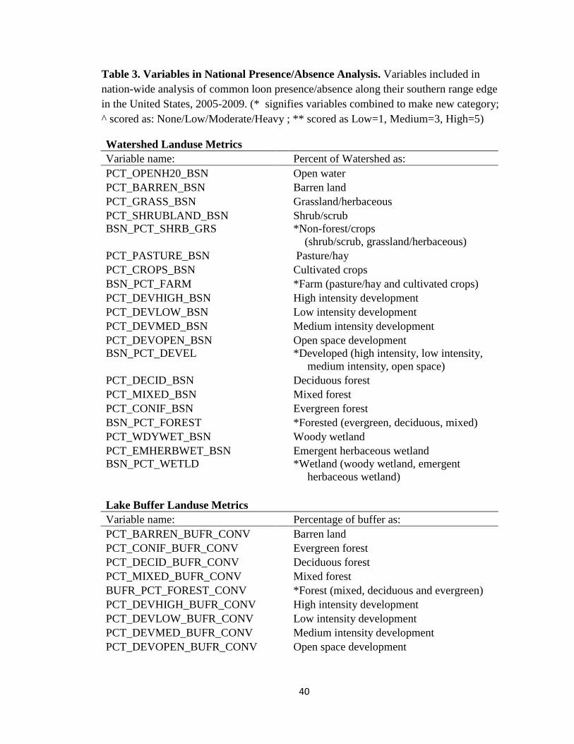
40

Table 3. Variables in National Presence/Absence Analysis. Variables included in

nation-wide analysis of common loon presence/absence along their southern range edge

in the United States, 2005-2009. (* signifies variables combined to make new category;

^ scored as: None/Low/Moderate/Heavy ; ** scored as Low=1, Medium=3, High=5)

Watershed Landuse Metrics

Variable name:

Percent of Watershed as:

PCT_OPENH20_BSN

Open water

PCT_BARREN_BSN

Barren land

PCT_GRASS_BSN

Grassland/herbaceous

PCT_SHRUBLAND_BSN

Shrub/scrub

BSN_PCT_SHRB_GRS

*Non-forest/crops

(shrub/scrub, grassland/herbaceous)

PCT_PASTURE_BSN

Pasture/hay

PCT_CROPS_BSN

Cultivated crops

BSN_PCT_FARM

*Farm (pasture/hay and cultivated crops)

PCT_DEVHIGH_BSN

High intensity development

PCT_DEVLOW_BSN

Low intensity development

PCT_DEVMED_BSN

Medium intensity development

PCT_DEVOPEN_BSN

Open space development

BSN_PCT_DEVEL

*Developed (high intensity, low intensity,

medium intensity, open space)

PCT_DECID_BSN

Deciduous forest

PCT_MIXED_BSN

Mixed forest

PCT_CONIF_BSN

Evergreen forest

BSN_PCT_FOREST

*Forested (evergreen, deciduous, mixed)

PCT_WDYWET_BSN

Woody wetland

PCT_EMHERBWET_BSN

Emergent herbaceous wetland

BSN_PCT_WETLD

*Wetland (woody wetland, emergent

herbaceous wetland)

Lake Buffer Landuse Metrics

Variable name:

Percentage of buffer as:

PCT_BARREN_BUFR_CONV

Barren land

PCT_CONIF_BUFR_CONV

Evergreen forest

PCT_DECID_BUFR_CONV

Deciduous forest

PCT_MIXED_BUFR_CONV

Mixed forest

BUFR_PCT_FOREST_CONV

*Forest (mixed, deciduous and evergreen)

PCT_DEVHIGH_BUFR_CONV

High intensity development

PCT_DEVLOW_BUFR_CONV

Low intensity development

PCT_DEVMED_BUFR_CONV

Medium intensity development

PCT_DEVOPEN_BUFR_CONV

Open space development

41

Table 3. Continued

Lake Buffer Landuse Metrics

Variable name:

BUFR_PCT_DEVEL_CONV

*Developed (high intensity, low intensity,

medium intensity, open space)

PCT_GRASS_BUFR_CONV

Grassland/herbaceous

PCT_SHRUBLAND_BUFR_CONV Shrub/scrub

BUFR_PCT_SHRB_GRS_CONV *Non-forest/crops (shrub/scrub,

grassland/herbaceous)

PCT_CROPS_BUFR_CONV

Cultivated crops

PCT_PASTURE_BUFR_CONV

Pasture/hay

BUFR_PCT_FARM_CONV

*Farm (pasture/hay, cultivated crops)

PCT_EMHERBWET_BUFR_CON

V Emergent werbaceous wetland

PCT_WDYWET_BUFR_CONV

Woody wetland

BUFR_PCT_WETLD_CONV

*Wetland (woody wetland, emergent

herbaceous wetland)

Lake Physical Characteristics

Variable name:

Variable Description:

DEPTHMAX

Maximum observed lake depth (m)

ELEV_PT

Site elevation (meters) from National

Elevation Dataset

LAKEAREA

Lake polygon area (km^2) from National

Elevation Dataset

LAKEPERIM

Lake polygon perimeter (km) from NHD

LEVEL_CHANGES

Elevation change (m) of lake level

MACRY_FLOAT

Emergent/floating coverage (% lake area)

MACRY_SUBMERGED

Submergent/floating coverage (% lake area)

PCT_EMRG_SUB_VEG

*Percent of submergent/floating,

emergent/floating coverage

SLD

Shoreline devel't index

(LAKEPERIM/(2*sqrt(LAKEAREA*pi))

LONG

Longitude

BASINAREA_HA

Watershed area

REGION

Region 1: NJ, VT, NH, NY, NJ, PA, RI, CT,

MA; Region 2: MI, OH, IL, IN, eastern WI;

Region 3: Western WI, IO, MN; Region 4:

WA, MT

42

Table 3. Continued

Lake Chemical Properties

Variable name:

Variable Description:

ANC

Gran ANC (ueq/L), Acid Neutralization

Capacity (ANC)

CL Chloride (ueq/L)

COLOR

Color (PCU)

COND

Conductivity (uS/cm @ 25 C)

CYANDENS

Cyanophyta density (#/cm2)

DO_FIELD

Field dissolved oxygen (mg/L)

DOC

Dissolved organic carbon (mg/L)

H

H+ from PH_LAB (ueq/L)

K

Potassium (ueq/L)

MCYST_TL_UGL

Total microcystin concentration (ug/L)

MG

Magnesium (ueq/L)

NA

Sodium (ueq/L)

NH4

Ammonium (ueq/L)

NO3

Nitrate (ueq/L)

NTL

Total nitrogen (ug/L)

OH

Hydroxide from PH_LAB (ueq/L)

PH_FIELD

Field pH from Profile DO data

(pH measured at first non-zero

depth unless only depth was zero)

PTL

Total phosphorus (ug/L)

SIO2

Silica (mg/L SiO2)

SO4

Sulfate (ueq/L)

TEMP_FIELD

Field water temperature (oC)

TURB

Turbidity (NTU)

Lake impacts and disturbances

Variable name:

Variable Description:

AGR_CROPLAND

^Agricultural cropland disturbances obs’d

AGR_FEEDLOT

^Agricultural feedlot

disturbances obs’d

AGR_LIVESTOCK

^Agricultural livestock disturbances obs’d

AGR_ORCHARDS

^Agricultural orchards disturbances obs’d

AGR_PASTURE

^Agricultural pasture disturbances obs’d

AGR_POULTRY

^Agricultural poultry disturbances obs’d

AGR_WITHDRAWL

Agricultural water withdrawl

AGR_IMPACT

*Summmed agricultural stressors

IND_SCORE

**Summed industrial stressor score

MAN_SCORE

**Summed lake management stressor score

43

Table 3. Continued

Lake impacts and disturbances

Variable name:

Variable Description:

REC_FILMS

^Recreational surface films, scums, slicks

disturbances obs'd

REC_MARINAS ^Recreational marinas disturbances obs’d

REC_PARKS

^Recreational parks disturbances obs’d

REC_PRIMITIVE

^Recreational primitive parks, camping

disturbances obs'd

REC_RESORTS

^Recreational resorts disturbances obs’d

REC_TRAILS

^Recreational hiking trails disturbances

observed

REC_TRASH

^Recreational trash/litter disturbances obs’d

REC_IMPACT

*Summed recreational stressors

RES_BRIDGES

^Recreational bridges/causeways

disturbances

observed

RES_CONSTRUCTION

^Recreational construction disturbances

obs’d

RES_DUMPING

^Residential dumping disturbances obs’d

RES_LAWNS

^Residential maintained lawns disturbances

obs’d

RES_PIPES

^Residential pipes, drains disturbances obs’d

RES_RESIDENCES

^Residential residences disturbances obs’d

RES_ROADS

^Residential roads disturbances obs’d

RES_SEWAGE

^Residential sewage treatment disturbances

obs’d

RES_IMPACT

*Summed residential stressors

Shoreline characteristics

Variable name:

Percentage of shoreline:

RCH_AGRICULTURE

agriculture

RCH_BARE_GROUND bare ground

RCH_FOREST

forest

RCH_GRASS

grass

RCH_SHRUB

shrub

RCH_WETLAND

wetland

RCH_DEVELOPMENT

development (Res & Urban)

RCH_SHOREMODS

modified (docks, riprap)

RCH_ALTERED

*human modification (development,

modified)

44

We compared the explanatory power of 112 lake characteristics, which we

characterized into six general categories: watershed land-use metrics, lake buffer land-use

metrics, lake physical characteristics, lake chemical properties, lake impacts and

disturbances, and shoreline characteristics (complete list: Table 7). We removed one lake

from consideration because of NLA data that were significantly outside the range of all

other lakes (Grubb’s test for one outlier, p < 10-16

). We also included two variables to

allow differential range determination by region (longitude and a categorical variable for

the four glacial lobes identified in Figure 4). To validate this approach for identifying

regional differences, we additionally constructed a decision tree for New England using

the same predictors from our continental model. The results from this tree agreed with

those from the continental model; therefore, we do not include further explanation of that

model in this chapter.

When creating the continental classification tree, we set the minimum number of

observations in a node to 30 before each split could be attempted and required the

resulting split to reduce the overall lack of fit by a cost complexity factor of 0.001. The

full tree explaining loon presence and absence was cross-validated ten times (using the

“xval” command within the “rpart” statement of R), and we then used the complexity

parameter to prune each tree to a size that minimized cross-validation error (Breiman et

al. 1984). We validated the pruned tree by running a random forest of 1000 trees from

the original dataset to assess the stability of our results. The “out-of-bag” (OOB) error

rate did not indicate that the random forest would have benefited from the addition of

more trees. Because there is no currently accepted standard for the number of predictors

that should be attempted at each node, we varied our values from 1 to 112 (in increments

45

of 10) and used the number of predictors that yielded the lowest OOB error rate (“mtry”

= 50; OOB error rate = 9.98%). Lastly, we created variable importance plots for all

predictor variables using both the decrease in mean Gini index value and the mean

decrease in model accuracy after the removal of each variable (calculated as the

normalized difference between the classification accuracy of the number of correctly

classified samples before the removal of a given variable from the number of correctly

classified samples after permutation, divided by the number of OOB samples for that

tree). This value was calculated for each of the 1000 trees in the random forest and its

average thus corresponds to the importance of a given variable in a model. We then

conducted partial dependence plots to explore the importance of top-ranked variables

within the random forest models.

2.3.3. Regional-scale Range Descriptors

The majority of lakes for which we had detailed demographic information were

not contained within the NLA database. We therefore constructed a decision tree using

the lakes of VT, NH, NY, and ME, but only considered the 20 variables that were

available for our lakes with demographic information as well (Table 4). These lake data

were compiled from the Environmental Protection Agency Wildlife Database Search

Engine (see “WDSE” for further information below).

46

Table 4. Variables in New England Presence/Absence Analysis. Variables included in

the analysis of common loon presence/absence along their southern breeding-range edge

in New England states, United States, 2005-2009.

Variable name Variable Description

BASINAREA_HA Watershed area

ELEV_PT Site elevation (meters) from National Elevation Dataset

DEPTHMAX Maximum observed lake depth (m)

LAKEAREA Lake polygon area (km^2) from National Elevation Dataset

LAKEPERIM Lake polygon perimeter (km) from NHD

CHLA Chloride (ueq/L)

PH_FIELD Total phosphorus (ug/L)

ANC Gran ANC (ueq/L), Acid Neutralization Capacity (ANC)

TURB Turbidity (NTU)

CL Chloride (ueq/L)

NO3 Nitrate (ueq/L)

SO4 Sulfate (ueq/L)

CA Calcium (ueq/L)

MG Magnesium (ueq/L)

NA Sodium (ueq/L)

K Potassium (ueq/L)

COLOR Color (PCU)

COND Conductivity (uS/cm @ 25 C)

DO_FIELD Field dissolved oxygen (mg/L)

PTL Total phosphorus (ug/L)

2.3.4. Regional Productivity Descriptors

We then constructed a decision tree to describe loon productivity across the

Northeastern United States. The Biodiversity Research Institute (BRI) has been

collecting data on loons throughout this region since 1987. The most continuous and

rigorous data are from the mountains of western Maine, beginning with work on 4 lakes

(12 loon territories) in 1993 (Dodge Lake, Quimby Lake, Rangeley Lake, and Round

Lake). Today, data are collected on 179 territories over 38 lakes in western Maine.

Additional data were included from New Hampshire (Loon Preservation Society),

Vermont (Vermont Center for Ecostudies), Massachusetts (MassWildlife, Massachusetts

47

Division of Conservation and Recreation), and New York (Biodiversity Research

Institute’s Adirondack Center for Loon Conservation and The Wildlife Conservation

Society’s Adirondack Program). Information from these sources was used to construct

our New England productivity decision tree.

We modeled the number of chicks surviving per pair (after four weeks of age)

using environmental lake characteristics found in the Environmental Protection Agency

Wildlife Database Search Engine (WDSE: http://oaspub.epa.gov/aed/wildlife.search). We

included 20 candidate variables from the WDSE (Table 5) that were measured

consistently across all lakes with productivity information. Loon productivity and lake

characteristics (when there were multiple entries for either) were averaged over each

decade for each lake (e.g. 1 80’s, 1 0’s, 2000’s). Averaging data by decade allowed us

to examine lakes on a fine spatial scale while correcting for individual loon-intrinsic or

seasonal variance in productivity or lake characteristics. The productivity means were

calculated across all territories within a lake, resulting in a continuous response variable

of average number of chicks per pair per lake for the decade, thus averaging out the

differences in productivity caused by either different individuals on different territories or

different territory holders across years. Tree construction operated similarly to the

previous models. We ran cross-validation ten times and plotted the cross-validation

error. We plotted the mean squared error (MSE) and total decrease in node impurity

(from splitting on a given variable) and our regression trees were substantiated with this

random forest model. We validated both of these models with random forests in the same

way we did our continental scale model.

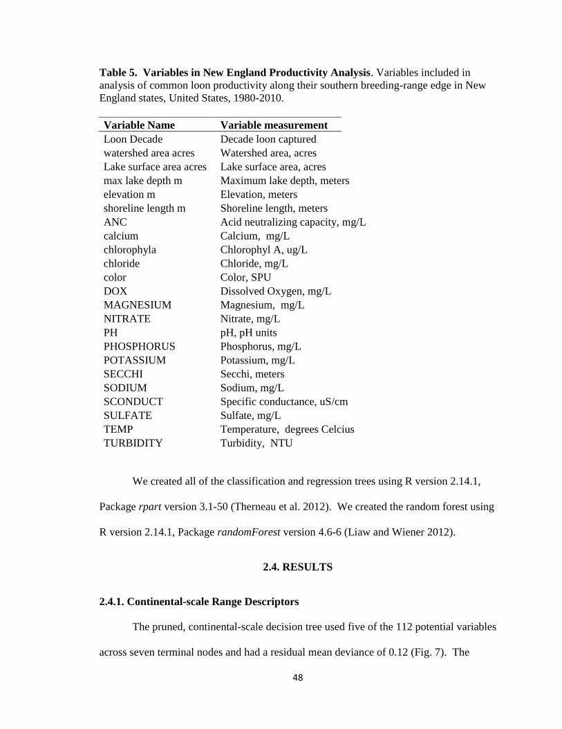
48

Table 5. Variables in New England Productivity Analysis. Variables included in

analysis of common loon productivity along their southern breeding-range edge in New

England states, United States, 1980-2010.

Variable Name Variable measurement

Loon Decade Decade loon captured

watershed area acres Watershed area, acres

Lake surface area acres Lake surface area, acres

max lake depth m Maximum lake depth, meters

elevation m Elevation, meters

shoreline length m Shoreline length, meters

ANC

Acid neutralizing capacity, mg/L

calcium

Calcium, mg/L

chlorophyla Chlorophyl A, ug/L

chloride

Chloride, mg/L

color

Color, SPU

DOX

Dissolved Oxygen, mg/L

MAGNESIUM Magnesium, mg/L

NITRATE

Nitrate, mg/L

PH

pH, pH units

PHOSPHORUS Phosphorus, mg/L

POTASSIUM Potassium, mg/L

SECCHI

Secchi, meters

SODIUM

Sodium, mg/L

SCONDUCT Specific conductance, uS/cm

SULFATE

Sulfate, mg/L

TEMP

Temperature, degrees Celcius

TURBIDITY Turbidity, NTU

We created all of the classification and regression trees using R version 2.14.1,

Package rpart version 3.1-50 (Therneau et al. 2012). We created the random forest using

R version 2.14.1, Package randomForest version 4.6-6 (Liaw and Wiener 2012).

2.4. RESULTS

2.4.1. Continental-scale Range Descriptors

The pruned, continental-scale decision tree used five of the 112 potential variables

across seven terminal nodes and had a residual mean deviance of 0.12 (Fig. 7). The

49

retained variables included lake water Na+ ion levels (ueq/L), lake surface area, SO4

(ueq/L) concentration, and lake elevation above sea level. For lakes with Na+ ion levels

greater than or equal to 144.3 ueq/L, loon presence was predicted positively by lower SO4

levels (threshold >= 67.68 ueq/L) and negatively by higher SO4 concentrations in the

lake. For lakes with Na+ of < 144.3 ueq/L, loons were absent on small lakes (threshold =

17.43 hectares), but in larger lakes loons were present on lakes at elevations greater than

529.2 meters above sea level and absent at lower elevation lakes.

Figure 7. United States Classification Tree. Pruned classification tree for common loon

presence/absence along the southern range edge, 2005-2009. Predicted values for splitting

decision (i.e. thresholds) and number of cases are presented at each node (absences / presences).

Predicted values of occupancy (0= absent, 1 = present) and number of cases are presented at each

terminal node. Each node (i.e. split) is shown as an inequality. If the inequality is true, follow

the left branch; if not proceed to the right branch.

Mean decreases in model accuracy and Gini indices for variables from each of the

random forest permutations (Fig. 8) largely agreed with our full, pruned tree, ranking Na+

and SO4 concentrations as the first and third most important variables, respectively. Lake

surface area also ranked high in importance for both the full tree and random forest

50

(ranked fourth and fifth by the Gini indices and mean decreases in accuracy respectively).

Chloride ion concentration was the second most important predictor in the random forest,

although it did not appear in our final classification tree. Scree plots of our two

importance rankings suggest either five (Gini Indicies) or six (Model Accuracy)

important variables overall, and include regional differences (longitude) and the percent

of mixed deciduous and coniferous forest in the drainage basin as important predictors

along with lake chemistry and size. Lake elevation was the tenth highest ranked, but was

not as strongly supported by the random forest models as the other top-ranking variables

identified by the continental classification tree (and likely correlates with forest cover in

the drainage basin).

The partial dependence plots of the six highest ranked predictorseach showed a

variety of threshold shapes for loon presence averaged over the effects of all other

variables (Fig. 9). At lower values of sulfate (SO4), chloride (Cl-), and sodium (Na

+), the

logit of probability of presence was high and then it decreased sharply (Fig. 11). An

increase in longitude (moving east) corresponded with an increase in the logit probability

of loon presence until - 4 longitude, after which the logit probability decreased steeply

until - 2 longitude. The logit probability of loon presence increased rapidly across small

lakes, and then leveled out after lakes larger than 100 hectares. The probability of loon

presence was low for values of mixed forest cover in the watershed until about 9%, after

which it increased rapidly.

51

Figure 8. Random Forest Analysis For United States. Mean decrease in accuracy and mean

decrease in Gini Index of first 33 variables for random forest model of presence/absence across

the continental United States using 112 predictive variables, 2005-2009. Variables higher on the

list are more important to explaining the response variable than those lower on the list. To

determine the mean decrease in accuracy, the prediction error on OOB data is subtracted from the

OOB error after permuting each predictor variable. These differences are averaged over the trees

(normalized by standard deviation of differences). The decrease in node impurity is the total

decrease in impurity from splitting on a given variable. To determine the mean decrease in Gini

Index (another impurity criterion), a score is assigned to a variable each time is used as one of the

primary splits in a tree. Gini Indexes are higher for the parent nodes than the descendent nodes,

thus high summed Gini indexes (the Gini Importance Measure) across the random forest

represent variables that occurred more commonly in higher nodes.

52

Figure 9. Dependence Plots for United States Analysis. Partial dependence plots give a

graphical representation of the marginal effect of a variable on the probability of presence or

absence, 2005-2009. These are partial dependence plots for the top six most important variables

for a continental analysis of common loon distribution along their southern range edge in the

United States.

2.4.2. Regional-scale Range Descriptors

Our final classification tree predicting loon presence or absence in New England

using the 20 WDSE candidate predictors consisted of 2 terminal nodes with a residual

mean deviance of 0.06 (Fig. 8). Again, Cl- concentration, an index of pH (acid

neutralization capacity instead of sulfate in this model), and lake surface area were

important variables for predicting loon distribution. Chloride concentration split the data

in half at a value of 158.3 ueq/L. At levels higher than this, the acid neutralization

53

capacity of the lake positively predicted presence (threshold = 754 ueq/L). At lower Cl-

concentrations lake surface area positively predicted loon presence (threshold = 33.9 ha).

Figure 10. Classification Tree For New England. Full and “pruned” (pruning is not justified

by cost-complexity analysis) classification tree: common loon presence/absence model for New

England states using a reduced number of predictive variables (20), United States, 2005-2009.

Predictors used in this model are the same as those used in the analysis of loon productivity in

New England. Predicted values for splitting decision (i.e. thresholds) and number of cases are

presented at each node. Predicted values for occupancy (0= absent, 1 = present) and number of

cases are presented at each terminal node. Each node (i.e. split) is shown as an inequality. If the

inequality is true, follow the left branch; if not proceed to the right branch.

The plotted mean decreases in accuracy and Gini indices for the variables in the

model showed that elevation, Na+ levels, and Cl

- levels were the most important variables

(the first splits of the trees, Fig. 11). We saw similar patterns for Na+ and Cl

-

concentrations in this smaller scale, reduced dataset as the continental scale tree where

each had low and abrupt thresholds for loon absence (negative relationship). Lake

magnesium, elevation, maximum depth, and surface area all had sharply increasing

relationships with the logit probability of presence (Fig. 12).

Tree

|CL>=158.3

ANC< 754 LAKEAREA< 0.3386

039/39

0

32/5

030/0

12/5

1

7/34

07/3

10/31

54

Figure 11. Random Forest For New England Analysis. Mean decrease in accuracy and mean

decrease in Gini Index of all 20 variables for random forest model of presence/absence in New

England, United States using 20 predictive variables, 2005-2009. Variables higher on the list are

more important to explaining the response variable than those lower on the list. For a full

description of the indices, see Fig. 8.

COLOR

NO3

PTL

CHLA

DO_FIELD

TURB

BASINAREA_HA

SO4

K

PH_FIELD

CA

COND

LAKEPERIM

ANC

DEPTHMAX

LAKEAREA

MG

CL

NA.

ELEV_PT

0.0 0.5 1.0 1.5 2.0

MeanDecreaseAccuracy

NO3

PTL

COLOR

DO_FIELD

CHLA

TURB

BASINAREA_HA

K

SO4

CA

COND

PH_FIELD

ANC

MG

DEPTHMAX

LAKEAREA

LAKEPERIM

CL

NA.

ELEV_PT

0 1 2 3 4 5

MeanDecreaseGini

pa.rf

55

Figure 12. Dependence Plots For New England Analysis. Partial dependence plots give a

graphical representation of the marginal effect of a variable on the probability of presence or

absence, 2005-2009. These are partial dependence plots for the top six most important variables

for the New England analysis of common loon distribution along their southern range edge in the

United States.

2.4.3. Regional Productivity Descriptors

Our full regression tree for the analysis of productivity in the New England

dataset used eight of the 20 candidate variables (eleven nodes) to construct the initial

classification tree; however, the pruned tree only retained two of these variables:

watershed size and lake surface area (Fig. 13). Lakes with smaller drainage basins

(threshold = 639.0 hectares) had lower loon productivity than lakes in larger drainage

0 1000 2000 3000

-0.2

0.2

NA.

0 500 1500 2500

-0.4

0.0

0.4

ELEV_PT

0 1000 2000 3000

-0.4

0.0

0.4

CL

0 1000 3000 5000-0

.20.1

MG

0 10 20 30 40 50

-0.2

0.1

LAKEAREA

0 10 20 30 40 50

-0.3

0.0

DEPTHMAX

56

basins, and these lakes had the lowest predicted productivity of the three terminal nodes

(1.2 chicks per pair per lake). Large lakes (threshold = 54.2 hectares) in larger drainage

basins had the highest productivity (1.8 chicks per pair per lake). tree for productivity model

Figure 13. Regression Tree For Productivity Model. Pruned regression tree: common loon

productivity model for loons in New England, United States, 1980-2010. Predicted values for

splitting decision (i.e. thresholds) and number of cases are presented at each node. Predicted

values for productivity (number of chicks per loon per decade) and number of cases are presented

at each terminal node. Each node (i.e. split) is shown as an inequality. If the inequality is true,

follow the left branch; if not proceed to the right branch.

For our random forest validation, our OOB error rate for our model was 13.2%,

which explained 42.4% of the variance. Drainage basin area, lake surface area, and

shoreline length were the highest ranked variables to split the data (Fig. 14). We were

unable to create partial dependence plots for the model as our original data contained too

many missing values (the tree itself is robust to these missing values (Breiman 2001) but

the partial dependence plotting procedure is not).

Pruned Regression Tree

|watershed.area.acres>=1579

Lake.surface.area.acres< 134

1.299n=126

1.18

n=94

1.65

n=32

1.347n=12

1.831n=20

57

TURBIDITYLoon.DecadechloridePOTASSIUMANCcalciumNITRATESULFATEMAGNESIUMDOXelevation.mSODIUMSCONDUCTSECCHIPHPHOSPHORUSchlorophylamax.lake.depth.mTEMPcolorshoreline.length.mLake.surface.area.acreswatershed.area.acres

0 5 10 15 20

%IncMSE

TURBIDITYLoon.DecadecalciumANCPOTASSIUMSODIUMchlorideSULFATENITRATESECCHIMAGNESIUMchlorophylaPHDOXSCONDUCTTEMPPHOSPHORUScolorelevation.mmax.lake.depth.mshoreline.length.mLake.surface.area.acreswatershed.area.acres

0 1 2 3 4 5

IncNodePurity

pa.narf

TURBIDITYLoon.DecadechloridePOTASSIUMANCcalciumNITRATESULFATEMAGNESIUMDOXelevation.mSODIUMSCONDUCTSECCHIPHPHOSPHORUSchlorophylamax.lake.depth.mTEMPcolorshoreline.length.mLake.surface.area.acreswatershed.area.acres

0 5 10 15 20

%IncMSE

TURBIDITYLoon.DecadecalciumANCPOTASSIUMSODIUMchlorideSULFATENITRATESECCHIMAGNESIUMchlorophylaPHDOXSCONDUCTTEMPPHOSPHORUScolorelevation.mmax.lake.depth.mshoreline.length.mLake.surface.area.acreswatershed.area.acres

0 1 2 3 4 5

IncNodePurity

pa.narf

Figure 14. Random Forest For Productivity Analysis. Percent increase in mean squared error

and increase in node purity all 20 variables for random forest model of productivity (continuous

response variable) in New England, United States using 20 predictive variables, 1980-2010.

Variables higher on the list are more important to explaining the response variable than those

lower on the list. These measures are analogous to the mean decrease in accuracy and Gini

Indices used for a binomial response variable.

58

2.5. DISCUSSION

2.5.1. Continental-scale Range Descriptors

Lake Na+ concentration, Cl

- , and SO4 were the most important predictors of loon

presence across the loon southern range edge in North America. The initial node with

Na+

identified 67% percent of the lakes without loons (tree: Fig. 9), and eliminated lakes

both within and outside the modern loon range. Our random forest analysis were

convergent with our pruned classification tree findings regarding the importance of Na+

(ranked most important variable in random forest; Fig. 8). Kuhn et al (2011) modeled

presence/absence in the New Hampshire and found that loons appeared to avoid human-

altered landscapes with high road densities and high levels of agricultural activity. A

similar process may be at work on a continental scale, as our results could be explained

by either a direct choice in Na+ levels, or the absence of other large landscape-level

disturbances, such as agriculture, development, or livestock grazing, which may alter lake

chemistry and increase Na+ levels (Dale 1997).

Lake Na+ concentration was the best indicator of continental loon distribution in

our random forest model (Fig. 10) and in our classification tree model. We do not

suspect this finding is due to an intolerance to Na+, as loons winter in marine

environments and have adaptations (e.g. large nasal glands, specialization of the kidneys)

to eliminate excess salt; however, further investigation into this realm is warranted. We

hypothesize instead that loons may be sensitive to the trophic effects of increased salinity

in freshwater ecosystems. Aside from natural variation in bedrock and net evaporation,

differences in lake Na+ levels are generally attributed to the runoff of road salt and

chemical deicers, which can elevate both Na+ and Cl

- levels in lakes (Rosenberry et al.

59

1999, Ramakrishna and Viraraghavan 2005) and suggests that loons may be less likely to

occur on lakes with high amounts of deicer application in the drainage basin. Across the

nation about 11 million tons of chemical deicers and road salts are spread each year

(Keating 2004), 85% of which are used in the mid-Atlantic, Great Lakes, and New

England states (Kaushal et al. 2005). This practice may be limiting the current

distribution of loons in these high-use regions. With climate change, interactions

between weather and human responses may alter this limitation. The average area of

snow cover in North America has decreased by 0. million square miles since the 1 0’s,

with the lowest value in 2006 (Armstrong and Brodzik 2006, Robinson and Heim Jr.

2006) and these trends are predicted to continue (Barnett et al. 2005). If the southern

distribution of loons is indeed limited by the ecosystem effects of road deicing, a warmer

world with less snow and ice may actually allow loons to recolonize some or all of their

former range. Alternatively, deicers may be a general index of human land use, as Cl-

concentration in lakes has also been linked to human disturbance in the drainage basin

(Herlihy et al. 1998). Under this scenario, we would not predict loon range expansion in

the near future, as human development is unlikely to reverse in the mid-Atlantic and

Midwest states.

Recent changes in the southern limit of the loon range support our initial

hypothesis. Historically, loons have been reported to breed in locations further south

than their current distribution in areas of northeast California, northern Iowa, southern

Minnesota, northern Illinois, southern Wisconsin, northern Indiana, southern Michigan,

northern Ohio, and northeast Pennsylvania where there are no modern records of

breeding (Evers et al. 2010). Loons began breeding in northern Massachusetts

60

approximately 40 years ago and in parts of Pennsylvania 30 years ago, both of which

represent either range expansions or a recolonization of their former range in these areas

(Evers et al. 2010) and may suggest a role for deicer application in current loon range

limitation.

Our variable dependence plots from the random forest model suggested a more

abrupt threshold for lake chemistry variables (such as Na+) than other landscape level

factors (Fig. 9). This pattern, however, may be attributed to correlations with other ions

that we did not test. For example the restriction of lake outflow creates a more saline

environment and increased levels of a large suite of ions (Wetzel 2005). Among the

twenty-four ions we tested (Table 8), however, Na+ repeatedly outperformed the others.

It is important to note that lakes with the highest Na+ concentrations were largely found

across the southern breeding range, suggesting that an untested correlate of latitude may

also be responsible for this pattern.

Another significant, positive predictor of loon occupancy was lake surface area.

Previous studies have analyzed lake surface area effects on loon occupancy and loon

reproductive success. Alvo et al (1988) found that lake surface area provided significant

discrimination between lakes where chicks were successfully raised versus where they

failed. In this study, lake surface area was related weakly but significantly to depth, and

neither depth nor surface area was related to water chemistry variables (as found in other

studies; Blenckner 2005). If lake surface area is driving the patterns with occupancy

directly, it is unlikely to change dramatically with climate change, although changes in

precipitation may change lake areas locally.

61

Loons may be sensitive to landscape-level forest changes, as three forest cover

variables were determined important in our top eight variables in our random forest

analysis (including one variable that our scree plot suggested was of the most important

variables). Climate change is expected to impact forest ecosystems in inconsistent ways

on varying spatial scales, with changes in disturbance regimes (Dale 1997) and plant

species ranges (Matthews 2004). A more immediate and likely change in many areas

across the northern United States over the next few decades will be from increased

population growth, local urbanization, and changes in ranching and farming practices

(Dale 1997). These land-use changes threaten to alter existing forested landscapes, which

may impact lake suitability for loon persistence. The percentage of mixed forest cover in

the drainage basin, however, primarily delineated northern lakes from southern lakes, and

therefore it is possible that the relationship we detected is driven by an untested factor

that also correlates with latitude (e.g. air temperature, day length, ice coverage).

While we would have ideally validated the results from our nationwide model

with a nationwide demographic model, this was not feasible due to incomplete data

across the entire southern range, a common constraint of demographically driven range

models. The strength of our approach, however, is that it allows for demographic

analysis in a portion of the range where these data are available. Creating an occupancy

model of the entire southern range allows for a comparison with the predictors from this

model with the variables that predict productivity in a portion of their southern range.

Further, creating an occupancy model for this same reduced area assures that any

differences detected are not due to a difference in scale rather than a difference in

mechanism.

62

2.5.2. Regional-scale Range Descriptors

To test whether the same factors influencing loon distribution on a continental

scale were operating on a regional scale, we analyzed data only for the lakes in New

York and New England states using fewer predictors. The variables retained (Cl-, acid

neutralizing capacity, and lake surface area) in the regional model were similar to those

retained on the national scale.

Cl- is a major anion in saline lakes (Wetzel 2005), and as the compound Na

+Cl

- is

a common road deicer, the identification of Cl- in this model may be analogous to the

importance of Na+ in our continental analysis. While coastal lakes can receive marine-

derived Cl- ions from atmospheric transport (Wetzel 2005), Cl

- increases are generally

due to pollution from road salt and municipal wastewaters (Sonzogni et al. 1983, Kaushal

et al. 2005).

A second variable, acid neutralizing capacity (ANC), was retained in our model

(ANC was a candidate predictor in the NLA dataset: Table 7). Total alkalinity levels are

a chief determinant of ANC (Wetzel 2005), and high alkalinity lakes are often more

biologically productive and less susceptible to the effects of acid precipitation (Driscoll et

al. 2003). Loons were largely present, therefore, on more productive lakes with higher

buffering capacities. The strength of the association between loon presence and ANC

value was not strong enough to be selected as a top predictor in the nationwide model, yet

in New England where lakes are categorized as “acid-sensitive” by the EPA (Driscoll et

al. 2003), the strength of this association was much more prominent. As our small-scale

models did not include lakes to the south of the current loon range boundary, however,

63

the inclusion of ANC in this tree may indicate that there are landscape characteristics that

predict unoccupied lakes within the range that are not predictive of the range edge itself.

While ANC appears to predict local lake occupancy and not larger scale range

edges, its local impact may increase with a changing climate. Although declines in

atmospheric sulfur dioxide emissions over the last several decades have helped to

increase ANC levels in lakes (Driscoll et al. 2003), climate-related events are reversing

this process (Laudon et al. 2004) via increased atmospheric acidic deposition (Magnuson

et al. 1997, IPCC 2007). Depending on position in the drainage basin, lakes that receive

less groundwater will be particularly vulnerable to acidification in drier years (Magnuson

et al. 1997). Predicted increases in summer drought intensity and frequency are expected

to increase acidic episodes in water bodies and cause declines in ANC (Laudon et al.

2004). Alterations in ANC, alkalinity, and lake pH could all have detrimental effects on

loon productivity and persistence on specific lakes within the loon range (McNicol et al.

1995).

2.5.3. Regional-scale Productivity Descriptors

Decadal productivity averages in New England were positively associated with

both drainage basin area and lake surface area. While lake surface area is unlikely to

change dramatically with climate change, lake surface area can indicate risks to nesting

success in the form of flash floods (which could inundate eggs) or droughts (which will

make it difficult for loons to push themselves across land to get to their nest) because of

correlations between lake size and position in the watershed. These potential climate

induced disturbances to nest success are, in fact, encountered to a lesser degree today

during extreme rainfall events or on reservoirs that draw water off quickly (Desorbo et al.

64

2007). Loon populations have persisted in most areas that experience these disturbances,

despite the increased challenge of successfully producing chicks (Evers et al. 2010).

Drainage basin size may be important due to its similar relationship to risk of lake level

variation or to other correlates with the land- cover of the drainage basin (e.g. forest

cover). Because drainage basin size and lake size were the most important factors in

predicting reproductive success, we are encouraged by the fact that these are not factors

that are likely to alter with climate change scenarios. If, however, these two variables are

important because of links with water-level variability, changes in precipitation regimes

may influence loon productivity by increasing or decreasing such risk.

While other studies have found patterns between loon productivity and the

variables we rejected (e.g. water clarity, water surface temperature, and dissolved organic

carbon), most of these studies were on a smaller scale. Undoubtedly, these correlations

between loon productivity and lake characteristics do exist, and may be important on a

smaller scale or within a single drainage basin. On a regional scale, however, the

individual effects did not predict the difference between occupied and unoccupied lakes.

2.5.4. Validating Envelope Models with Hierarchical Decision Trees

Our goals were to identify variables that were important in determining

distribution and productivity and distinguish which variables were important in one

realm, the other, or both. Our smaller scale presence/absence model identified subsets of

the continental drivers of loon range edge and thus relationships appear to vary across

space, but continental scale decision trees capture smaller-scale relationships. Lake

salinity (measured by Na+ or Cl

-), acidity (measured by SO4 or ANC), and surface area,

were all important in determining loon presence at both a continental and regional scale.

65

Our productivity model validated the demographic underpinning of two variables as

loon range predictors: lake surface area and drainage basin size. Forest composition of

the drainage basin was a consistent predictor of loon presence at both regional scale and,

to a lesser degree, the continental scale. Forest composition is driven by variables that

are scale dependent (e.g. substrate, climate, graving, site history, etc. vary on a local

versus site scale (Corney et al. 2006). Although we did not directly test forest

composition in our productivity model, the only drainage basin variable we did test,

drainage basin size, was an important predictor of loon productivity. This underscores

the demographic importance of the drainage basin to loons and suggests a possible

demographic mechanism for its power as a range predictor.

Our method of pairing our occupancy model with a demographic model made us

more confident in our occupancy model results. The productivity model rejected lake

salinity and acidity as predictors. While these two predictors appeared important at both

the regional and continental scales, we found no ties with offspring production. This

does not mean, of course, that there is no demographic underpinning to these two

variables. They may influence settling rate (immigration) or apparent site fidelity

(emmigration and survival). On the other hand, they may be spurious due to correlations

with another demographically important variable. Our approach allowed us to reject their

linkage with productivity, and further investigations could test for linkages with other

demographic mechanisms. Without the hierarchical validation, however, we would not

have been able to distinguish between the two predictors that were related to productivity

and the two predictors that were not.

66

2.5.5. Implications for Climate Change on the Range of the Common Loon

Our overall findings regarding the probability of loon persistence within the

United States are promising. All of our demographically validated variables that explain

loon distribution are unlikely to change with climate, although we need a better

understanding of how drainage basin composition and lake size influences productivity to

be confident. Of the range predictors that were not related to loon productivity, two were

unlikely to change greatly due to climate (salinity and acidity/alkalinity). In both of these

cases, however, we need to be conservative in our predictions until we understand why

these characteristics predict the current loon range. If they are not validated through a

demographic mechanism other than productivity, these relationships may be spurious and

their predictive ability for future range shifts severely limited. Smaller scale studies have

suggested demographic linkages between loons and acidity/alkalinity, but we recommend

additional large-scale investigations to validate this lake characteristic at a continental

scale. Overall, however, we believe our generalized approach of a continental envelope

model followed by smaller scale machine learning techniques to validate the

demographic underpinnings of important variables represents a distinct step forward in

developing range models that will accurately predict range shifts with landscape and

climate change. In this case study we were able 1) to reject or support the productivity

underpinnings of range predictors from an envelope model and 2) reject the ability of a

number of variables, which were previously identified as important for loon demography,

to predict the current range of the common loon. This approach should work equally well

with many species to identify variables that are both accurate predictors of current ranges

and tied to demographic mechanisms likely to lead to range changes in the future.

67

It is important to recognize that our analysis only addresses loon persistence in the

United States during a portion of their annual cycle. Loons that breed in the continental

United States spend the entirety of their winter on the Atlantic or Pacific Oceans, or, less

commonly, on unfrozen freshwater systems near the ocean (Evers et al. 2010). Future

changes in ocean conditions that lower winter survival or energy stores required for

migration and subsequent breeding may have larger impacts on the common loon

breeding range than changes directly to breeding lakes themselves.

68

CHAPTER 3

BLOOD METABOLITES AS INDICATORS OF BREEDING HABITAT

QUALITY: A SENSITIVE METHOD TO PREDICT RANGE

ALTERATION UNDER CLIMATE CHANGE?

3.1 ABSTRACT

Climate change has the potential to shift and/or restrict species’ ranges. While

previous studies have generally failed to predict range alteration successfully, individual

energetic condition may offer more potential because it can identify covariance between

energetic condition and breeding habitat quality. We used blood metabolites and

behavioral observations to evaluate the energetic costs of common loons (Gavia immer)

breeding on lakes across a gradient of environmental, spatial, and behavioral conditions.

Using these physiological and behavioral endpoints we created a framework for

evaluating the effect of environmental characteristics on the value of breeding locations

along the species’ southern range edge (ME, NH, MA, MT, WA). Using samples

collected over two years (n=97), blood triglyceride concentrations suggest that the

number of chicks, breeding latitude, and daily temperature are important predictors of

loon energy expenditure. Specifically we found that: 1) loons with two chicks expend

more energy than those with one, 2) loons near the southern range edge expend more

energy to produce a given brood size than those nearer the range center and, 3) birds

breeding in warmer temperatures expend more energy than those in cooler temperatures

(controlling for year, territory type, and calendar date, free glycerol levels, size-corrected

body mass, and longitude). We suggest that as environmental conditions change in the

69

coming years, blood metabolites offer a promising predictor of population collapse along

range boundaries.

3.2 INTRODUCTION

Climate change is predicted to cause a range of effects on animal populations

(IPCC 2007). In birds, the potential for range shifts, expansions, and contractions has

already been realized by numerous species (Watkinson et al. 2004, Waite and Strickland

2006, Virkkala et al. 2008, Barbet-Massin et al. 2009, Martinez-Morales et al. 2010).

Some of the hypothesized mechanisms behind these shifts include changes in food

availability, phenological alignment, and thermoregulatory challenges (Brown et al.

1999, Walther et al. 2002).

One of the most common ways to predict how climate will alter bird species’

distributions is through the use of bioclimatic envelope models. These models link the

current geographical distribution of a species to climatic variables, and the predicted

locations of these variables are then used to forecast the species’ occurrence (Heikkinen

et al. 2006). Most researchers agree that this method is only a first step in determining

the predicted changes in distribution, and it should only be used as a guideline for further

investigation (Pearson and Dawson 2003, Hampe 2004, Stanley and Royle 2005, Hijmans

and Graham 2006, Heikkinen et al. 2006, Vallecillo et al. 2009) as distributions may not

be limited simply by climate (Beale et al. 2008). Models that link species’ ranges to

explicit ecological and demographic processes have proven more useful in predicting the

effects of habitat degradation (from climate or other rapid landscape changes) on animal

distributions (Holt and Keitt 2005, Byrd 2012, Chpt. 2). Metrics that influence the

70

demographic processes underlying range edges are the most valuable for determining

how alterations in these parameters may change future distributions.

In order to link an organism’s distribution with an individually based mechanism

of distribution change, it is important to examine the relationship between physiology and

environment. Linking physiology to microclimatic data in a scalable way is the key to

understanding a species’ distribution (Hodkinson 1999). Species-specific physiological

thresholds of temperature, for example, are known to limit the distribution of a wide

variety of organisms (Nickerson et al. 1988, Walther et al. 2002, Pörtner 2002), and it is

reasonable therefore to assume that we can detect initial differences in metabolic

expenditure under thermal conditions that are less extreme than those needed to cause

local extirpation. This initial variance could then potentially act as a harbinger of larger

scale population changes.

Body mass is a widely used estimate of energy stores as it is noninvasive and easy

to measure, and changes in body mass can give an indication of changes in energy stores

(Jenni-Eiermann and Jenni 1994). This method of determining stores of fat reserves,

however, has shortcomings. These include the need to recapture animals (e.g. energy

stores might influence recapture ability) and the potentially adverse affects of capture on

fat acquisition (Jenni-Eiermann and Jenni 1994).

Blood metabolites are one potentially useful link between environmental

conditions and individual energetic expenditure that can shed light on an individual’s

ability to deal with changing environmental conditions (Brown et al. 1999). Plasma

metabolites are the products of intermediary metabolism and are measured in the

bloodstream between their origin within an organ and their delivery to another location in

71

the body (Jenni-Eiermann and Jenni 1998). Therefore, concentrations of plasma

metabolites relate to both the current energetic demand of an individual and the

individual’s ability to meet that demand. Very high triglyceride levels, for instance, can

indicate that an individual is increasing caloric intake or fat reserves (which may suggest

that it is more buffered from environmental changes; Quillfeldt et al. 2004). Conversely,

triglycerides are hydrolyzed during fasting (to increase fatty acid and glycerol

availability), and thus lower triglyceride levels and elevated glycerol typify fasting (or

possibly starvation) in birds (Carey 1996). Overall, plasma metabolites can be viewed as

correlates of the net balance of stored energy from the preceding hours (Jenni-Eiermann

and Jenni 1998).

We examined free glycerol and triglyceride concentrations in the blood of

brooding common loons (Gavia immer) to assess the energetic demand of birds in

different environments along the species’ southern range extent. We predicted that we

would detect low glycerol values with little variation in our population of successfully

breeding loons (captured at night during fasting). Free glycerol has shown no nightly or

diurnal trend in birds fasting through the night (Jenni-Eiermann and Jenni 1997) and

concentrations were generally low in a study of garden warblers (Sylvia borin) when an

individual’s body mass was increasing or when fat reserves were stable (Jenni-Eiermann

and Jenni 1994). In this same study, triglyceride levels followed the opposite pattern

where the highest values occurred during fattening and the lowest values occurred during

fat loss. Because our loons were successfully breeding, we assumed that they were in

relatively high condition (low glycerol and higher triglycerides). Because we caught

them all during their nightly fast, we expected varying concentrations of triglycerides as a

72

function of net energy assimilation and use from the previous day. Therefore, we

predicted that we would see differences in triglyceride levels which would indicate

energetic state. This same link between fat reserves and triglyceride levels has been

found in two studies of fasting gulls (Totzke et al. 1999, Alonso-Alvarez and Ferrer

2001). Further, a study of reed warblers (Jenni and Schwilch 2001) concluded that

triglyceride levels were better predictors of changes in lipid stores than overall change in

body mass. Finally, while a study of thirteen species of seabirds near Shumigan Island,

Alaska found no differences in triglyceride levels in various stages of breeding condition,

all of our samples were collected from loons that were brooding chicks to control for

variation due to breeding stage.

In the past several decades, the population growth rates of common loons (Gavia

immer) have declined in several regions of the northern United States (Sidor et al. 2003,

Karasov et al. 2007, Evers et al. 2008, Grear et al. 2009) and the collapse of populations

in this southern portion of the range has been predicted by a bioclimatic envelope model

(Matthews 2004). The best predictors for both loon distribution and seasonal

productivity in North America, however, are fairly robust to near-term changes in climate

and are more sensitive to human disturbance (e.g. forest cover in the drainage basin, Na+

levels in a lake, lake surface area: Byrd 2012, Chpt. 2). We expect, however, that if

range contraction along the southern extent of the loon distribution occurs due to changes

in the breeding environment, the cost of reproduction will increase prior to the

appearance of measurable changes in demographic variables such as offspring production

or bird abundance. Demographic models agree that changes in factors affecting adult

survival are more likely to cause population change than variation in fecundity directly

73

(Grear et al. 2009). Evaluating the energetic demand of breeding adults will help to

understand the conditions within the current breeding range that are most likely to affect

population viability and cause range contractions.

To construct a more physiologically mechanistic model of common loon

persistence, we examined the way in which environmental and social parameters at

different scales varied with the blood triglyceride concentration of individuals on the

breeding grounds, controlling for glycerol concentrations. These relationships may then

identify environmental variables that impact adult survival and control both loon

population viability and drive range changes. Here, we examine common loon

triglyceride levels to link environmental variance with energetic condition during what

we believe is one of the most energetically demanding portions of the loon life cycle,

chick rearing.

3.3 MATERIALS AND METHODS

3.3.1. Study Population, Field Methods, and Lab Assays

Loon captures took place between May and August of 2010 and 2011. Blood

samples were collected in Maine (n= 77), New Hampshire (n= 22), New York (n= 4),

Washington (n = 4), and Montana (n= 4). Breeding adults with chicks were captured at

least 30 minutes after evening civil twilight using both spotlighting and playback

recordings (Evers 1992, 2001b). To identify individuals in the future, loons were fitted

with unique color bands in addition to a USGS issued metal band. All individuals were

of known sex, were caring for chicks, and were captured at night (i.e. were fasting: Evers

et al. 2010). Standard morphometric measurements were taken (e.g. tarsus width, weight,

bill length) to create an index of body size (Senar and Pascual 1997). Within fifteen

74

minutes of capture, we collected a blood sample in a heparinized capillary tube following

the venipuncture of the metatarsal vein. The samples were kept on ice until centrifuged

(within six hours) at 6000 rpm for 10 minutes. Plasma was frozen until laboratory assays

were performed.

We conducted triglyceride/free glycerol assays to determine the levels of free

glycerol, total glycerol, and triglycerides from blood samples. Assays were conducted in

accordance with the Triglyceride/Free Glycerol Assay Protocol from the Holberton

Laboratory of Avian Biology (Holberton 2008). Using a colorimetric enzymatic endpoint

assay we measured plasma glycerol levels (GPO-Trinder Assay, kit 337; B Sigma-

Aldrich, St. Louis, Missouri). Plasma samples were run in duplicate using 96-well plates

and read on a SpectraCount reader (Packard, Palo Alto, California). We used a

commercial standard of known triglyceride levels and created a standard curve to

standardize our results.

3.3.2. Behavioral Observations

We recruited biologists from four Northeastern states to gather behavioral

observations of 113 loon territories. In particular we were interested in the frequency of

escalation of territorial interactions. We expected that one of the most energetically

expensive activities in which territorial birds could engage would be territorial disputes.

During these interactions, territorial birds (both males and females) may chase intruders

around the lake at high speed while “rowing” with their wings on the surface of the

water. They may also physically grapple, beating their wings against one another and

attempting to spear their opponents with their bills (Piper et al. 2000, 2008b, Evers et al.

2010). Not all interactions escalate to this level, however, and interactions may end after

75

as little as a vocal call and some slight changes in posture. Territorial defense in birds

may account for 0.9 to 33.1% of daily energy expenditure during the height of the

breeding season (Walsberg 1983). While 41.5% of territory acquisitions in loons occur

through passive takeover (desertion or death of previous territory holder), the same

percentage of acquisitions occur through the active displacement of a member of the

resident pair or through earlier arrival time at the territory (Piper et al. 2000). Thus,

defense of a territory has the potential to require a large portion of a loon’s seasonal

energetic budget.

We hypothesized that the likelihood of an intense escalation was at least partially

a function of the energetic condition of the territory holder. Biologists across New

Hampshire, New York, Vermont, Massachusetts, and Maine recorded the frequency of

territorial intrusions and the level of escalation of an interaction by the territory holder

(“passive”: intruder is present but territory holder is not currently engaged in an

aggressive interaction or “active”: territory holder is having an aggressive interaction

with intruder including peering, circle dancing, pursuing, directly physically contacting

intruder, directly vocalizing at intruder, or other) from May-August of 2010 and 2011.

Loons were observed from the lakeshore or from a kayak and the first behavior observed

by the researcher were recorded. Behaviors were recorded separately for both members

of the pair and marked individuals were differentiated when possible.

3.3.3. Statistics

In order to determine the average triglyceride and free glycerol levels in our

samples, we used Microsoft Office Excel (2007) to find the mean and standard deviation

of our measures.

76

We identified 17 candidate variables a priori that made biological sense based on

field observations, exploratory data analysis, and published literature. Candidate

predictors of loon condition explained variation in the immediate landscape (2), in the

larger region (2), in the local social environment (3), in the timing of the sample (6), and

among individuals (4).

We identified four spatial variables. Our two landscape-scale effects included

drainage basin area and lake surface area, both of which are landscape-level predictors of

loon productivity (Byrd 2012, Chpt. 2). Lake surface area may correlate with several

social parameters, as well. Nocera and Burgess (2002) found that lake surface area was

positively correlated with dive-pause times and variation in dive-pause times, which they

speculated was because loons on larger lakes may be more apt to encounter intruders

(through interactions with adjacent territory holders as well as loons from other lakes)

and therefore must remain on the surface for longer periods to successfully defend their

territory. Additionally, larger lakes potentially support a greater number and diversity of

nesting locations and habitat variation, which may be preferred by loons. The information

for the lake attribute fields was gathered from the Environmental Protection Agency

Wildlife Database Search Engine (http://oaspub.epa.gov/aed/wildlife.search) and the

USGS National Water Information System (http://nwis.waterdata.usgs.gov). We also

accounted for spatial variation at the regional scale by including latitude and longitude

(decimal degrees).

We included three characteristics of the social environment previously found to

influence loon behavior. First, we characterized each loon territory as one of three types.

Loons breed on multiple lake territories (where their territory is comprised of many

77

lakes), whole lake territories (where there is one pair of loons on one lake), and partial

lake territories (where more than one pair is on a given lake; Evers et al. 2010). All of

the territories in this study were either whole lake or partial lake types. We predicted that

loons on single-lake territories would encounter lower energetic demands as they do not

defend shared territory boundaries with other pairs, nor do they need to fly to other lakes

to meet their nutritional requirements, as they do on multi-lake territories (Piper et al.

1997b). Second, we included both the number of pairs on the lake and the interaction

between number of pairs and lake surface area to account for potential increases in

territorial interactions with bird density on various lake sizes.

We accounted for temporal variation in the triglyceride concentration by

including six potential variables. We included the sampling year to account for year-to-

year variation and julian date to control for seasonal variation. To account for the

potential impacts of the local weather prior to sampling on triglyceride levels, we

included the minimum and maximum daily temperature (to the nearest tenth of a degree

C) on the day prior to the night of capture and the two, two-way interactions between

temperature (minimum and maximum) and year to account for variation in this

relationship among years. Weather data were collected from the National Oceanic and

Atmospheric Administration’s National Climatic Data Center

(http://www.ncdc.noaa.gov/) from the closest land-based weather station with historical

data for the day in question.

Lastly we included four variables that controlled for intrinsic individual

differences. We included sex to detect possible differences between male and female

triglyceride levels (e.g. energetic demands of incubation; (Williams 1996, Thomson et al.

78

1998, Evers et al. 2010; or territory defense; Piper et al. 2008) and the number of chicks

produced (1 or 2) to account for potential differences in the energetic demands of

different brood sizes (Deerenberg et al. 1995, Lozano and Lemon 1998). As body mass

is an important variable for interpreting metabolite results (Jenni-Eiermann and Jenni

1994), we included size-corrected body mass (weight/tarsus) in our model. Lastly, we

included free glycerol concentration as a candidate predictor, because the relationship

that circulating triglycerides have with free glycerol can help explain the stage of fat

acquisition or depletion that an organism is experiencing (Jenni-Eiermann and Jenni

1994, Guglielmo et al. 2005).

Candidate models were all repeated-measures, mixed-effects models (LMM)

using maximum likelihood (“ML”; package ‘nlme’ in R 2.14.1; Jose Pinheiro et al. 2011)

with the lake of capture was a random effect. Model selection was conducted using

stepwise AIC model selection (“stepAIC”, package ‘MASS’ in R 2.14.1; (Venables and

Ripley 2009), using backward selection. Optimal variance and correlation structures for

the models were selected using Akaike’s Information Criterion (AIC) values (Pinheiro

and Bates 2000, Zuur et al. 2009), and models with ∆AIC < 2.0 were considered

equivalent.

For our analysis of behavioral data, we used Microsoft Office Excel (2007) to

determine the mean and standard error of our observations.

3.4 RESULTS

3.4.1. Establishing Baseline Metabolic Measures

Loons of differing mass were largely homogenous in energetic condition which

allowed us to define the values for energetic regulation of known breeding individuals.

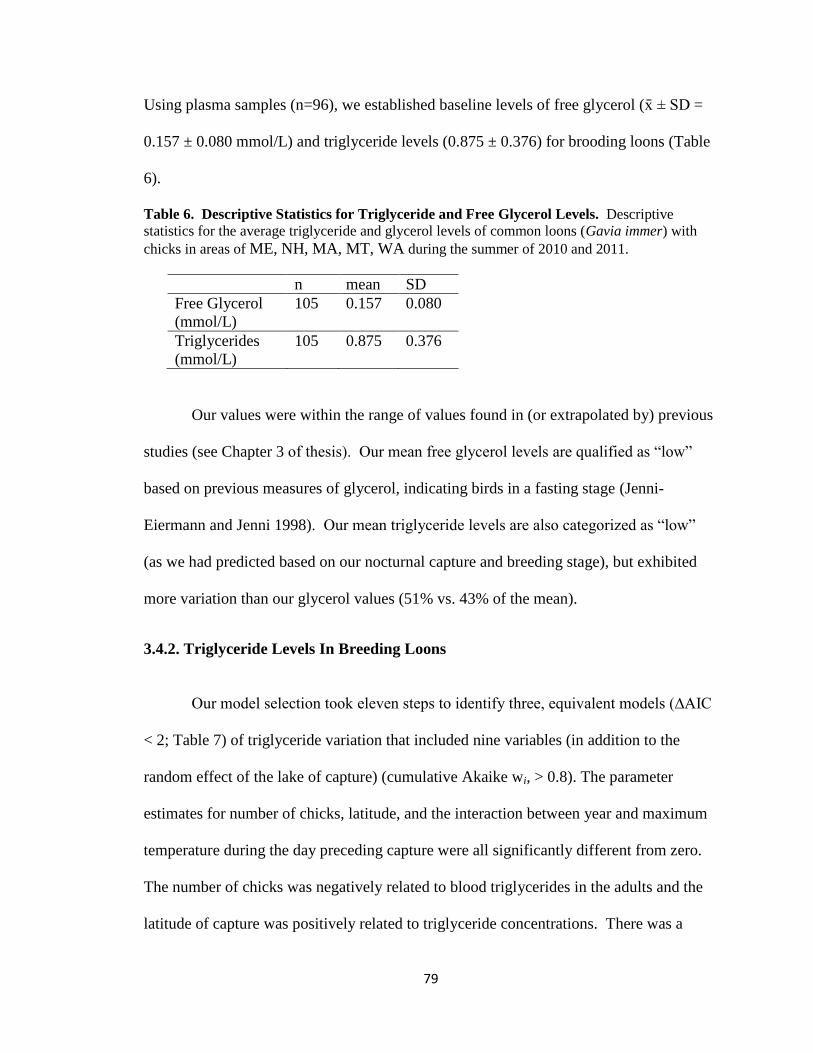
79

Using plasma samples (n=96), we established baseline levels of free glycerol (x SD =

0.157 ± 0.080 mmol/L) and triglyceride levels (0.875 ± 0.376) for brooding loons (Table

6).

Table 6. Descriptive Statistics for Triglyceride and Free Glycerol Levels. Descriptive

statistics for the average triglyceride and glycerol levels of common loons (Gavia immer) with

chicks in areas of ME, NH, MA, MT, WA during the summer of 2010 and 2011.

n mean SD

Free Glycerol

(mmol/L)

105 0.157 0.080

Triglycerides

(mmol/L)

105 0.875 0.376

Our values were within the range of values found in (or extrapolated by) previous

studies (see Chapter 3 of thesis). Our mean free glycerol levels are qualified as “low”

based on previous measures of glycerol, indicating birds in a fasting stage (Jenni-

Eiermann and Jenni 1998). Our mean triglyceride levels are also categorized as “low”

(as we had predicted based on our nocturnal capture and breeding stage), but exhibited

more variation than our glycerol values (51% vs. 43% of the mean).

3.4.2. Triglyceride Levels In Breeding Loons

Our model selection took eleven steps to identify three, equivalent models (∆AIC

< 2; Table 7) of triglyceride variation that included nine variables (in addition to the

random effect of the lake of capture) (cumulative Akaike wi, > 0.8). The parameter

estimates for number of chicks, latitude, and the interaction between year and maximum

temperature during the day preceding capture were all significantly different from zero.

The number of chicks was negatively related to blood triglycerides in the adults and the

latitude of capture was positively related to triglyceride concentrations. There was a

80

significant negative relationship between the highest maximum temperatures and

triglycerides in 2011 but not in 2010. Akaike weights for the top three models (out of

eleven potential models) were 32.4%, 26.2%, and 24.1% respectively (Table 7). Number

of chicks, year, territory type, latitude, free glycerol levels, maximum temperature, and

the interaction of year and maximum temperature were found in all eleven models. We

employed model averaging of the eleven models to create parameter estimates as a way

to include model selection uncertainty into these values (Table 5). Model selection

indicated that the inclusion of julian date, year, free glycerol levels, and longitude

improved model support, but the 95% confidence intervals of these parameter estimates

included zero, making it difficult to gauge their strength (Table 8).

Size-corrected body mass had no influence on triglyceride levels (was not a

covariate in our top three models). A post-hoc analysis showed no relationship between

triglyceride levels and the residuals of size-corrected body mass (r2= 0.003).

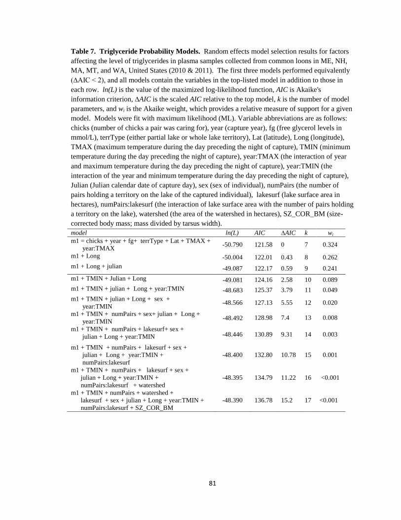
81

Table 7. Triglyceride Probability Models. Random effects model selection results for factors

affecting the level of triglycerides in plasma samples collected from common loons in ME, NH,

MA, MT, and WA, United States (2010 & 2011). The first three models performed equivalently

(∆AIC < 2), and all models contain the variables in the top-listed model in addition to those in

each row. ln(L) is the value of the maximized log-likelihood function, AIC is Akaike's

information criterion, ∆AIC is the scaled AIC relative to the top model, k is the number of model

parameters, and wi is the Akaike weight, which provides a relative measure of support for a given

model. Models were fit with maximum likelihood (ML). Variable abbreviations are as follows:

chicks (number of chicks a pair was caring for), year (capture year), fg (free glycerol levels in

mmol/L), terrType (either partial lake or whole lake territory), Lat (latitude), Long (longitude),

TMAX (maximum temperature during the day preceding the night of capture), TMIN (minimum

temperature during the day preceding the night of capture), year:TMAX (the interaction of year

and maximum temperature during the day preceding the night of capture), year:TMIN (the

interaction of the year and minimum temperature during the day preceding the night of capture),

Julian (Julian calendar date of capture day), sex (sex of individual), numPairs (the number of

pairs holding a territory on the lake of the captured individual), lakesurf (lake surface area in

hectares), numPairs:lakesurf (the interaction of lake surface area with the number of pairs holding

a territory on the lake), watershed (the area of the watershed in hectares), SZ_COR_BM (size-

corrected body mass; mass divided by tarsus width).

model ln(L) AIC ∆AIC k wi

m1 = chicks + year + fg+ terrType + Lat + TMAX +

year:TMAX -50.790 121.58 0 7 0.324

m1 + Long -50.004 122.01 0.43 8 0.262

m1 + Long + julian -49.087 122.17 0.59 9 0.241

m1 + TMIN + Julian + Long -49.081

124.16 2.58 10 0.089

m1 + TMIN + julian + Long + year:TMIN -48.683

125.37 3.79 11 0.049

m1 + TMIN + julian + Long + sex +

year:TMIN -48.566 127.13 5.55 12 0.020

m1 + TMIN + numPairs + sex+ julian + Long +

year:TMIN -48.492

128.98 7.4 13 0.008

m1 + TMIN + numPairs + lakesurf+ sex +

julian + Long + year:TMIN -48.446 130.89 9.31 14 0.003

m1 + TMIN + numPairs + lakesurf + sex +

julian + Long + year:TMIN +

numPairs:lakesurf

-48.400 132.80 10.78 15 0.001

m1 + TMIN + numPairs + lakesurf + sex +

julian + Long + year:TMIN +

numPairs:lakesurf + watershed

-48.395 134.79 11.22 16 <0.001

m1 + TMIN + numPairs + watershed +

lakesurf + sex + julian + Long + year:TMIN +

numPairs:lakesurf + SZ_COR_BM -48.390 136.78 15.2 17 <0.001

82

Table 8. Triglyceride Model-Averaged Parameter Estimates. Parameter estimates from

original 11 models and model-averaged parameter estimates with unconditional 95% confidence

intervals for variables in the top three models for triglyceride levels in common loons (Gavia

immer) in ME, NH, MA, MT, and WA, 2010 and 2011. Parameters considered include the

number of chicks (0 or 1), year (2010 or 2011), territory type (single lake or shared lake), capture

date (Julian), latitude and longitude of capture lake, maximum temperature on day of capture, and

the interaction between year and maximum temperature. Values in the parentheses following

each variable name indicate the reference level for binomial variables. Model-averaged

parameters whose estimates are significantly different from zero are in bold text.

Variable fixed effects

coefficient 95% CI

Chicks -0.209 -0.3935, -0.0264

Year (2011) 1.202 -0.2816, 2.6844

Territory Type

(partial-lake territory) -0.221 -0.4848, 0.0433

Julian -0.005 -0.0128, 0.0024

free glycerol 0.929 -0.3824, 2.2413

Degrees North Latitude 0.125 0.0467, 0.3826

Degree East Longitude 0.012 -0.0052, 0.0293

Maximum Temperature on Previous Day 0.001 -0.0026, 0.0040

Year (2011) x Maximum Temp -0.006 -0.0122, -0.0001

3.4.3. Behavior

Among 1228 observations of 113 loon territories, we recorded 56 incidences of

territorial intrusion on 32 territories. Only a single territorial pair ever exhibited both

escalated and un-escalated (i.e. active and passive) territorial behaviors. For the 22 loon

pairs for which both behavioral data and metabolite samples were collected, eight showed

territorial behaviors, and loons that escalated interactions had lower plasma triglyceride

concentrations than those that did not (Table 9), although the sample size is quite small.

83

Table 9. Descriptive statistics for the average triglyceride levels of common loons (Gavia immer)

with intruding loons on their territory that either did not respond aggressively (passive) or

responded with some degree of aggression (excalating) in ME, NH, MA during the summer of

2010 and 2011.

x n SE

passive 0.957 3 0.1365

escalating 0.784 5 0.0225

3.5 DISCUSSION

Our triglyceride levels suggest the loons we captured were in a fasting stage

(lower overall triglyceride values, i.e. <2.0 mmol/L), which is corroborated by the timing

of our sampling (nocturnal sampling in a diurnal foraging species). Within our range of

values, loons with lower triglycerides have higher energetic demand as they are utilizing

and mobilizing lipids more rapidly than the birds with higher plasma triglyceride levels

(Jenni-Eiermann and Jenni 1998, Nagy et al. 1999, Price et al. 2008). Loons that

escalated interactions had lower blood triglyceride concentrations pointing to an

increased cost in escalating interactions with intruding males, as suggested by previous

studies (Piper et al. 2000)

Our models suggested that energetic demand in breeding loons is influenced by

factors on various scales. Our top-ranked models suggest that energetic condition as

assessed by triglycerides is a function of a loon’s individual breeding effort (the number

of chicks produced), region (latitude, longitude), and weather conditions (maximum

temperature and the interaction of year and temperature), controlling for the social

environment (territory type), other metabolites (glycerol), and the time of sampling

(julian capture date, year).

84

The number of chicks a loon cared for was negatively related to triglyceride

values (when controlling for other variables in the model), which suggests that within our

range of values, loons with one chick are less energetically taxed than those with two.

Similar to our results, Deerenberg et al. (1995) found an increase in daily energy

expenditure in European kestrels (Falco tinnunculus) with increased clutch size. More

indirectly, decreases in mass are frequently reported during breeding in birds (for a

review see Moreno 1989), suggesting increases in energetic demand are related to

offspring production. This increase in energetic demand is likely a function of the

required rate of provisioning, which is a function of brood size (Jodice et al. 2006,

Gingras and Paszkowski 2006, Enstipp et al. 2007). Loon chicks are completely

dependent on their parents for food during the first several days of life. By three weeks

of age, they can chase fish for upwards of 30 meters, however their capture rate is still

poor (3%), and parents supply chicks with most of their food until nearly eleven weeks of

age (Gingras and Paszkowski 2006, Evers et al. 2010). Yellow warblers (Dendroica

petechia) increase both their provisioning rate and energetic demand when clutch size is

experimentally increased (Lozano and Lemon 1998), and a similar mechanism is likely at

play in our system. Our results, therefore, suggest that a future drop in the number of

loons brooding two versus one chick may signal an underlying physiological inability to

care for a larger brood, which could signify larger shifts toward population inviability.

What is unknown in our study species is how previous breeding experience impacts

current breeding condition at a given brood size as has been shown in common terns

(Sterna hirundo; Bauch et al. 2010).

85

Latitude was positively associated with triglyceride levels in our sample of loons,

indicating that at more northern sites, loons face decreased energetic demand. Our

latitude values ranged from 43.2 ˚ N to 48.8 ˚N. Basal metabolic rate has been shown to

correlate positively within vertebrate phylogenies with latitude (Weathers 1979, 1997,

Weathers and Greene 1998). Our results are contrary to this larger pattern, but it is

difficult to determine whether this is due to the relatively small latitudinal range over

which we conducted the study or whether this is indeed a physiological symptom of a

range edge. Collecting metabolites over a wider range of latitudes and along northern as

well as southern range edges would help illuminate the generality of this trend.

Our results indicated that triglyceride levels were negatively related to maximum

daily temperature on the day of capture on a given year (Fig. 15), suggesting that higher

maximum temperature produced lower energetic demand in 2011 (while controlling for

the other variables in the model, including latitude). Energy expenditure has been

reported to decrease with ambient temperature in other bird species as well (Claudia

Rauter and Reyer 2000). The strong relationship between metabolic demand and

temperature was present only in 2011. We assume that the metabolic demand of loons is

even more tightly tied to water temperature, since heat loss by endotherms in water is

higher than in air at the same temperature due to the thermal conductivity of water

(Jenssen et al. 1988). While water birds have mechanisms for increased thermoregulation

owing to their aquatic lifestyle (e.g. plumage insulation, peripheral vasoconstriction),

minimal thermal “wet” conductance in some waterbirds can be as much as 5 % greater

than conductance due to air (Jenssen et al. 1988). Unfortunately, we did not record

surface water temperatures during capture. As mean global temperature increases (IPCC,

86

2007), however, loons may be more energetically taxed due to higher maximum

temperatures during the chick rearing stage. Additionally, incubation is a

thermoregulatory challenge for loons and other birds under warm temperatures (Eppley

1996). The loons within our study area regularly pant during incubation (which suggests

they are above their thermal neutral zone), suggesting that higher temperatures may

impact the overall cost of breeding more dramatically outside of the chick rearing stage.

Higher temperatures over the long term will also likely influence prey species

abundances and biomass (Ficke et al. 2007). Additionally, higher surface water

temperatures will increase the strength and duration of lake stratification (Peeters et al.

2007), altering lake communities and food-web dynamics (Ficke et al. 2007). While

loons are adapted to surviving on various different prey items (Evers et al. 2010), large-

scale shifts in prey composition could potentially push loons out of once suitable

breeding lakes regardless of any decrease in energetic expenditure on thermal regulation.

87

Figure 15. Temperature/Year Interaction Plot. An all-effects plot examining the relationship

of year and temperature on triglyceride levels in common loons (Gavia immer), May- August,

2010-2011. Maximum temperature values on capture days ranged from 16.6-32.2 degrees C in

2010 and 17.9-35.0 degrees C in 2011. The relationship with the highest maximum temperatures

is shown in the upper plot and lowest maximum temperature in the lower plot.

3.6 SUMMARY

Breeding birds must optimize the allocation of energy into self-maintenance and

parental care (Martins and J 1993, Pettifor 1993) in the face of varying climatic

conditions and food resources (Claudia Rauter and Reyer 2000). Blood triglyceride

concentrations suggest that the number of chicks, breeding latitude, and daily temperature

are important predictors of loon energy expenditure (controlling for year, territory type,

and calendar date, free glycerol levels, size-corrected body mass, and longitude).

Specifically we found that: 1) loons with two chicks expend more energy than those with

one, 2) loons near the southern range edge expend more energy to produce a given brood

size than those nearer the range center and, 3) birds breeding in warmer temperatures

expend more energy than those in cooler temperatures (controlling for year, territory

88

type, and calendar date, free glycerol levels, size-corrected body mass, and longitude).

Without taking further measures of physiology, biologists can monitor maximum

temperature across years, and chick number (and latitude, if examining larger areas) and

identify areas of vulnerability before reproduction halts entirely. Of critical importance

as climate changes is monitoring changes in maximum temperature. While our findings

suggest that warmer temperatures may reduce the cost of thermoregulation for breeding

loons, our concern is in regards to the ways that temperature is predicted to negatively

impact hydrologic systems. Together these results suggest that common loons may be

sensitive to increases in temperature along their southern range boundary. Previous

investigations of southern range determinants using either brood counts or bird presence

did not detect similar patterns, which suggests that physiological measures may be more

sensitive indicators of range contractions than more traditional bioclimatic envelope or

demographic approaches.

89

BIBLIOGRAPHY

Alonso-Alvarez, C., and M. Ferrer. 2001. A biochemical study of fasting, subfeeding, and

recovery processes in yellow-legged gulls. Physiological and biochemical zoology

74:703–13.

Alvo, R., D. Hussell, and M. Berrill. 1988. The breeding success of common loons (

Gavia immer ) in relation to alkalinity and other lake characteristics in Ontario.

Canadian Journal of Zoology 66:746–752.

Armstrong, R. L., and M. J. Brodzik. 2006. Northern Hemisphere Snow Extent Derived

from Microwave and Optical Satellite Data. Pages 1–7. . Boulder, Colorado.

Badzinski, S. S., and S. T. A. Timmermans. 2006. Factors influencing productivity of

common loons (Gavia immer) breeding on circumneutral lakes in Nova Scotia,

Canada. Hydrobiologia 567:215–226.

Barbet-Massin, M., B. a Walther, W. Thuiller, C. Rahbek, and F. Jiguet. 2009. Potential

impacts of climate change on the winter distribution of Afro-Palaearctic migrant

passerines. Biology letters 5:248–51.

Barnett, T. P., J. C. Adam, and D. P. Lettenmaier. 2005. Potential impacts of a warming

climate on water availability in snow-dominated regions. Nature 438:303–9.

Barr, J. F. 1973. Feeding biology of the Common Loon (Gavia immer) in oligotrophic

lakes of the precambrian shield. . Univ. of Guelph, Ontario.

Bauch, C., S. Kreutzer, and P. H. Becker. 2010. Breeding experience affects condition:

blood metabolite levels over the course of incubation in a seabird. Journal of

comparative physiology. B, Biochemical, systemic, and environmental physiology

180:835–45.

Beale, C. M., J. J. Lennon, and A. Gimona. 2008. Opening the climate envelope reveals

no macroscale associations with climate in European birds. Proceedings of the

National Academy of Sciences of the United States of America 105:14908–12.

Blair, R. B. 1992. Lake Features, Water Quality and the Summer Distribution of

Common Loons in New Hampshire. Distribution 63:1–9.

Blenckner, T. 2005. A conceptual model of climate-related effects on lake ecosystems.

Hydrobiologia 533:1–14.

Breiman, L. 2001. Random Forests. Machine Learning 45:5–32.

Breiman, L., J. Friedman, C. J. Stone, and R. A. Olshen. 1984. Classification and

Regression Trees. . Chapman & Hall/CRC.

90

Brown, J. L., S. H. Li, and N. Bhagabati. 1999. Long-term trend toward earlier breeding

in an American bird: a response to global warming? Proceedings of the National

Academy of Sciences of the United States of America 96:5565–69.

Byrd, A. J., B. J. Olsen, D. C. Evers, and R. L. Holberton. 2012. Common Loon (Gavia

immer) Biogeography & Reproductive Success in an Era of Climate Change.

Carey, C. 1996. Avian Energetics and Nutritional Ecology. Pages 324–374. . Chapman &

Hall/CRC, New York, New York, USA.

Chase, M. K., N. Nur, and G. R. Geupel. 2005. Effects of Weather and Population

Density on Reproductive Success and Population Dynamics in a Song Sparrow

(Melospiza melodia ) Population : A Long-Term Study. The Auk 122:571–592.

Claudia Rauter, and H. Reyer. 2000. Thermal and energetic consequences of nest location

and breeding times in Water Pipits (Anthus spinoletta). Journal of Ornithology

141:391–407.

Corney, P. M., M. G. Le Duc, S. M. Smart, K. J. Kirby, R. G. H. Bunce, and R. H. Marrs.

2006. Relationships between the species composition of forest field-layer vegetation

and environmental drivers, assessed using a national scale survey. Journal of

Ecology 94:383–401.

Crawley, M. 2007. The R Book. . Wiley, Chichester, England; Hoboken, N.J.

Cutler, D. R., T. C. Edwards, K. H. Beard, A. Cutler, K. T. Hess, J. Gibson, and J. J.

Lawler. 2007. Random forests for classification in ecology. Ecology 88:2783–92.

Dale, V. 1997. The Relationship Between Land-Use Change and Climate Change.

Ecological Applications 7:753–769.

Davis, A. J., L. S. Jenkinson, J. H. Lawton, B. Shorrocks, and S. Wood. 1998a. Making

mistakes when predicting shifts in species range in response to global warming.

Nature 391:783–786.

Davis, A. J., J. H. Lawton, B. Shorrocks, and L. S. Jenkinson. 1998b. Individualistic

species responses invalidate simple physiological models of community dynamics

under global environmental change. Journal of Animal Ecology 67:600–612.

Deerenberg, C., I. Pen, C. Dijkstra, B.-J. Arkies, G. H. Visser, and S. Daan. 1995.

Parental energy expenditure in relation to manipulated brood size in the european

kestrel. Zoology, Analysis of Complex Systems (ZACS) 99:38–47.

Desorbo, C. R., K. M. Taylor, D. E. Kramar, J. Fair, J. H. Cooley, D. C. Evers, W.

Hanson, H. S. Vogel, and J. L. Atwood. 2007. Reproductive Advantages for

Common Loons Using Rafts. Journal of Wildlife Management 71:1206–1213.

91

De’ath, G., and K. Fabricius. 2000. Classification and regression trees: a powerful yet

simple technique for ecological data analysis. Ecology 81:3178–3192.

Doligez, B., E. Danchin, J. Clobert, and L. Gustafsson. 1999. The use of conspecific

reproductive success for breeding habitat selection in a non-colonial, hole-nesting

species, the collared flycatcher. Journal of Animal Ecology 68:1193–1206.

Drilling, N. E., and C. F. Thompson. 1988. Natal and breeding dispersal in house wrens

(troglodytes-aedon). Auk 105:480–491.

Driscoll, C. T., K. M. Driscoll, K. M. Roy, and M. J. Mitchell. 2003. Chemical response

of lakes in the Adirondack Region of New York to declines in acidic deposition.

Environmental science & technology 37:2036–42.

Dyke, A. S., and V. K. Prest. 1987. Late Wisconsinan and Holocene History of the

Laurentide Ice Sheet. Geographie physique et Quaternaire 41:2.

Enstipp, M. R., D. R. Jones, S.-H. Lorentsen, and D. Grémillet. 2007. Energetic costs of

diving and prey-capture capabilities in cormorants and shags (Phalacrocoracidae)

underline their unique adaptation to the aquatic environment. Journal of Ornithology

148:593–600.

Eppley, Z. A. 1996. Society for Experimental Biology Seminar Series 59. Pages 313–346

Development of Thermoregulation in Birds: physiology, interspecific variation and

adaptation to climate.

Evers, D. C. 1992. A replicable capture method for adult and juvenile common loons on

their nesting lakes. Proc. From the 1992 conference on the loon and its ecosystem:

Status, management, and environmental concerns.:214–220.

Evers, D. C. 2001a. Common Loon Population Studies: Continental Mercury Patterns

and Breeding Territory Philopatry. . Univ. of MN, St. Paul, MN.

Evers, D. C. 2001b. Common Loon Population Studies: Continental Mercury Patterns

and Breeding Territory Philopatry.

Evers, D. C., J. D. Paruk, J. W. McIntyre, and J. F. Barr. 2010. Common Loon (Gavia

immer).

Evers, D. C., L. J. Savoy, C. R. DeSorbo, D. E. Yates, W. Hanson, K. M. Taylor, L. S.

Siegel, J. H. Cooley, M. S. Bank, A. Major, K. Munney, B. F. Mower, H. S. Vogel,

N. Schoch, M. Pokras, M. W. Goodale, and J. Fair. 2008. Adverse effects from

environmental mercury loads on breeding common loons. Ecotoxicology (London,

England) 17:69–81.

92

Ewert, D. 1982. Spring migration of Common Loons at Whitefish Point, Michigan. Jack-

Pine Warbler 60:134–143.

Ficke, A. D., C. a. Myrick, and L. J. Hansen. 2007. Potential impacts of global climate

change on freshwater fisheries. Pages 581–613 Reviews in Fish Biology and

Fisheries.

Gaston, K. J. 2003. The structure and dynamics of geographic ranges. Oxford University

Press.

Gingras, B., and C. a. Paszkowski. 2006. Feeding behavior and modeled energetic intake

of common loon (Gavia immer) adults and chicks on small lakes with and without

fish. Hydrobiologia 567:247–261.

Gostomski, T. J., and D. C. Evers. 1998. Time-activity budget for Common Loons, Gavia

immer, nesting on Lake Superior. Canadian Field-Naturalist 112:191–197.

Grear, J. S., M. W. Meyer, J. H. Cooley, A. Kuhn, H. Walter, M. G. Mitro, H. S. Vogel,

K. M. Taylor, K. P. Kenow, S. M. Craig, D. E. Nacci, A. Press, and S. Grear. 2009.

Population Growth and Demography the Northern United States of Common Loons

in. The Journal of Wildlife Management 73:1108–1115.

Greenwood, P. J., and P. H. Harvey. 1982. The natal and breeding dispersal of birds.

Annual Review of Ecology and Systematics 13:1–21.

Guglielmo, C. G., D. J. Cerasale, and C. Eldermire. 2005. A field validation of plasma

metabolite profiling to assess refueling performance of migratory birds.

Physiological and biochemical zoology 78:116–25.

Hampe, A. 2004. Bioclimate envelope models : what they detect and what they hide.

Global Ecology & Biogeography 13:469–476.

Heikkinen, R. K., M. Luoto, M. B. Araujo, R. Virkkala, W. Thuiller, and M. T. Sykes.

2006. Methods and uncertainties in bioclimatic envelope modelling under climate

change. Progress in Physical Geography 30:751–777.

Hemberger, M., D. Euler, and J. Barr. 1983. The impact of cottage development on

common loon reproductive success in central Ontario. Wilson Bulletin 95:431–439.

Herlihy, A. T., J. L. Stoddard, and C. B. Johnson. 1998. The relationship between stream

chemistry and watershed land cover data in the mid-atlantic region, U.S. Water, Air,

and Soil Pollution 105:377–386.

Hijmans, R. J., and C. H. Graham. 2006. The ability of climate envelope models to

predict the effect of climate change on species distributions. Global Change Biology

12:2272–2281.

93

Hitch, A. T., and P. L. Leberg. 2007. Breeding distributions of north American bird

species moving north as a result of climate change. Conservation biology : the

journal of the Society for Conservation Biology 21:534–9.

Hodkinson, I. D. 1999. Species response to global environmental change or why

ecophysiological models are important: a reply to Davis et al. Journal of Animal

Ecology 68:1259–1262.

Holberton, R. L. 2008. Matericals and basic methods for field blood collection, storage,

etc. . Orono, ME.

Holt, R. D., and T. H. Keitt. 2005. Species ’ borders : a unifying theme in ecology. Oikos

108:3–6.

Holt, R. D., T. H. Keitt, M. A. Lewis, B. A. Maurer, and M. L. Taper. 2005. Theoretical

models of species ’ borders : single species approaches. Oikos 108:18–27.

IPCC. 2007. Contribution of Working Group I to the Fourth Assessment Report of the

Intergovernmental Panel on Climate Change. Page 996 (S. D. Solomon, M. Qin, M.

Manning, Z. Chen, M. Marquiz, K. B. Averyt, M. Tignor, and H. L. Miller, Eds.). .

Cambridge University Press, United Kingdom and New York.

Jacobson, G. L., I. J. Fernandez, P. A. Mayewski, and C. V. Schmitt. 2009. Maine’s

Climate Future: An Initial Assessment. . Orono.

Jenni, L., and R. Schwilch. 2001. Plasma metabolite levels indicate change in body mass

in reed warblers Acrocephalus scirpaceus. Avian Science 1:55–65.

Jenni-Eiermann, S., and L. Jenni. 1994. Plasma Metabolite Levels Predict Individual

Body-Mass Changes in a Small Long-Distance Migrant , the Garden Warbler

Author. The Auk 111:888–899.

Jenni-Eiermann, S., and L. Jenni. 1997. Diurnal Variation of Metabolic Responses to

Short-Term Fasting in Passerine Birds during the Postbreeding , Molting and

Migratory Period. The Condor 99:113–122.

Jenni-Eiermann, S., and L. Jenni. 1998. What can plasma metabolites tell us about the

metabolism, physiological state and condition of individual birds? An overview.

Biological Conservation Fauna 102:312–319.

Jenssen, B. M., M. Ekker, and C. Bech. 1988. Thermoregulation in winter-acclimatized

common eiders (Somateria mollissima) in air and water. Canadian Journal of

Zoology 67:669–673.

94

Jodice, P. G. R., D. D. Roby, R. M. Suryan, D. B. Irons, K. R. Turco, E. D. Brown, J. F.

Thedinga, and G. H. Visser. 2006. Increased energy expenditure by a seabird in

response to higher food abundance. Marine Ecology Progress Series 306:283–293.

Jose Pinheiro, D. Bates, S. DebRoy, and D. Sarkar. 2011. nlme: Linear and Nonlinear

Mixed Effects Models. R package version 3.1-106.

Karasov, W. H., K. P. Kenow, M. W. Meyer, and F. Fournier. 2007. Bioenergetic and

pharmacokinetic model for exposure of common loon (Gavia immer) chicks to

methylmercury. Environmental toxicology and chemistry / SETAC 26:677–85.

Kaushal, S. S., P. M. Groffman, G. E. Likens, K. T. Belt, W. P. Stack, V. R. Kelly, L. E.

Band, and G. T. Fisher. 2005. Increased salinization of fresh water in the

northeastern United States. Proceedings of the National Academy of Sciences of the

United States of America 102:13517–20.

Keating, J. 2004. Deicing Salt: Still on the Table. Stormwater.

Kenow, K. P. K., D. A. Dams, N. Schoch, D. Evers, W. Hanson, D. Yates, L. Savoy, T.

Fox, A. Major, R. Kratt, J. Ozard, R. O. K. Ratt, and J. O. H. N. O. Zard. 2009.

Migration Patterns and Wintering Range of Common Loons Breeding in the

Northeastern United States. Waterbirds 32:234–247.

Kenow, K. P., M. W. Myer, R. K. Hines, and W. I. H. K. Karasov. 2007. Distribution and

accumulation of mercury in tissues of captive-reared common loon ( gavia immer )

chicks. Environmental toxicology and chemistry / SETAC 26:1047–1055.

Kingston, J. D., A. L. Deino, R. K. Edgar, and A. Hill. 2007. Astronomically forced

climate change in the Kenyan Rift Valley. Journal of Human Evolution 53:487–503.

Kuhn, A., J. Copeland, J. Cooley, H. Vogel, K. Taylor, D. Nacci, and P. August. 2011.

Modeling Habitat Associations for the Common Loon ( Gavia immer ) at Multiple

Scales in Northeastern North America. Avian Conservation and Ecology 6.

Lathrop, R. C., S. R. Carpenter, and D. M. Robertson. 1999. water clarity responses to

phosphorus , Daphnia grazing , and internal in Lake Mendota mixing. Limnology

and Oceanography 44:137–146.

Laudon, H., P. J. Dillon, M. C. Eimers, R. G. Semkin, and D. S. Jeffries. 2004. Climate-

induced episodic acidification of streams in central ontario. Environmental science

& technology 38:6009–15.

Liaw, A., and M. Wiener. 2012. Package “randomForest”. . CRAN.

95

Lozano, G. A., and R. E. Lemon. 1998. Parental-care responses by yellow warblers

(Dendroica petechia) to simultaneous manipulations of food abundance and brood

size. Canadian Journal of Zoology 76:916–924.

Mager, J. N., and C. Walcott. 2007. Structural and contextual characteristics of territorial

“yodels” given by male Common Loons (Gavia immer) in northern Wisconsin.

Passenger Pigeon 69:327–337.

Mager, J. N., C. Walcott, and W. H. Piper. 2007. Male Common Loons, Gavia immer,

communicate body mass and condition through dominant frequencies of territorial

yodels. Animal behaviour 73:683–690.

Magnuson, J. J., K. E. Webster, R. A. Assel, C. J. Bowser, P. J. Dillon, J. G. Eaton, H. E.

Evans, E. J. Fee, R. I. Hall, L. R. Mortsch, D. W. Schindler, and F. H. Quinn. 1997.

Potential effects of climate changes on aquatic systems : laurentian great lakes and

precambrian shield region. Hydrological Processes 11:825–871.

Martinez-Morales, M. A., I. Zuria, L. Chapa-Vargas, I. MacGregor-Fors, R. Ortega-

Alvarez, E. Romero-Aguila, and P. Carbo. 2010. Current distribution and predicted

geographic expansion of the Rufous-backed Robin in Mexico: a fading endemism?

Diversity and Distributions 16:786–797.

Martins, T., and W. J. 1993. Cost of reproduction and allocation of food between parent

and young in the swift (Apus apus). Behavioral Ecology 4:213±223.

Matthews, S. N. 2004. Atlas of climate change effects in 150 bird species of the Eastern

United States. . US Department of Agriculture, Forest Service, Northeastern

Research Station.

McIntyre, J. W. 1994. Loons in freshwater lakes. Hydrobiologia 279-280:393–413.

McIntyre, J. W. ., and J. F. . Barr. 1983. Pre-Migratory Behavior of Common Loons on

the Autumn Staging Grounds. Wilson Ornithological Society 95:121–125.

McNicol, D. K., M. L. Mallory, and H. S. Vogel. 1995. Using volunteers to monitor the

effects of acid precipitation on common loon (Gavia immer) reproduction in canada:

the canadian lakes loon survey. Water, Air, and Soil Pollution 85:463–468.

Moreno, J. 1989. Strategies of mass change in breeding birds. Biological Journal of the

Linnean Society:297–310.

Nagy, K. a, I. a Girard, and T. K. Brown. 1999. Energetics of free-ranging mammals,

reptiles, and birds. Annual review of nutrition 19:247–77.

96

Newman, S. H., J. F. Piatt, and J. White. 1997. Hematological and Plasma Biochemical

Reference Ranges of Alaskan Seabirds : Their Ecological Significance and Clinical

Importance. Colonial Waterbirds 20:492–504.

Nickerson, D. M., D. E. Facey, and G. D. Grossman. 1988. Estimating Physiological

Thresholds with Continuous Two-Phase Regression. Physiological Zoology 62:866–

887.

Nocera, J. J., and N. M. Burgess. 2002. Diving schedules of Common Loons in varying

environments. Canadian Journal of Zoology 80:1643–1648.

Olson, S. T., and W. H. Marshall. 1952. The Common Loon in Minnesota.

O’Connor, R. J., and T. L. Wagner. 2004. a Test of a Regression-Tree Model of Species

Distribution. The Auk 121:604.

Parker, K. E. 1988. Common Loon Reproduction and Chick Feeding on Acidified Lakes

in the Adirondack Park, New York. Canadian Journal of Zoology 66:804–810.

Paruk, J. D. 2009. Function of the common loon foot waggle. The Wilson Journal of

Ornithology 121:392–398.

Payne, R. B., and L. L. Payne. 1993. Breeding dispersal in Indigo Buntings:

circumstances and consequences for breeding success and population structure.

Condor 95:1–24.

Pearson, R. G., and T. P. Dawson. 2003. Predicting the impacts of climate change on the

distribution of species : are bioclimate envelope models useful ? Global Ecology &

Biogeography 12:361–371.

Peeters, F., D. Straile, A. Lorke, and D. Ollinger. 2007. Turbulent mixing and

phytoplankton spring bloom development in a deep lake. Limnology and

Oceanography 52:286–298.

Pettifor, R. A. 1993. Brood-manipulation experiments II. A cost of reproduction in blue

tits (Parus caeruleus)? Journal of Animal Ecology 62:145–159.

Pinheiro, J. C., and D. M. Bates. 2000. Mixed-effects models in S and S-PLUS. . New

York: Springer.

Piper, W. H., D. Evers, M. W. Meyer, K. B. Tischler, D. Kaplan, and R. C. Fleischer.

1997a. Genetic monogamy in the common loon (Gavia immer). Behavioral Ecology

and Sociobiology 41:25–31.

97

Piper, W. H., J. D. Paruk, D. C. Evers, M. W. Meyer, B. Keren, M. Klich, and J. J.

Hartigan. 1997b. Local Movements of Color-Marked Common Loons. The Journal

of Wildlife Management 61:1253–1261.

Piper, W. H., C. Walcott, J. N. Mager, and F. J. Spilker. 2008a. Nestsite selection by

male loons leads to sex-biased site familiarity. Journal of Animal Ecology 77:205–

210.

Piper, W. H., C. Walcott, J. N. Mager, and F. J. Spilker. 2008b. Fatal battles in common

loons: a preliminary analysis. Animal Behaviour 75:1109–1115.

Piper, W., K. Tischler, and M. Klich. 2000. Territory acquisition in loons: the importance

of take-over. Animal behaviour 59:385–394.

Poff, N. L. 2002. Ecological response to and management of increased flooding caused

by climate change. Philosophical transactions. Series A, Mathematical, physical, and

engineering sciences 360:1497–510.

Pokras, M. A., C. Hanley, and Z. Gordon. 1998. Liver mercury and methylmercury

concentrations in New England common loons (Gavia immer). Environmental

Toxicology and Chemistry 17:202–204.

Price, E. R., A. Krokfors, and C. G. Guglielmo. 2008. Selective mobilization of fatty

acids from adipose tissue in migratory birds. The Journal of experimental biology

211:29–34.

Pörtner, H. O. 2002. Climate variations and the physiological basis of temperature

dependent biogeography: systemic to molecular hierarchy of thermal tolerance in

animals. Comparative biochemistry and physiology. Part A, Molecular & integrative

physiology 132:739–61.

Quillfeldt, P., J. F. Masello, and E. Mostl. 2004. Blood chemistry in relation to nutrition

and ectoparasite load in Wilson’s storm-petrels Oceanites oceanicus. Polar Biology

27:168–176.

Ramakrishna, D. M., and T. Viraraghavan. 2005. Environmental Impact of Chemical

Deicers – A Review. Water, Air, and Soil Pollution 166:49–63.

Robinson, D. A., and R. R. Heim Jr. 2006. Trends and variability of snowfall and snow

cover across north america and eurasia. Part 2: what the data say. Pages 1–5. .

Asheville, NC.

Rodenhouse, N. L., S. N. Matthews, K. P. McFarland, J. D. Lambert, L. R. Iverson, a.

Prasad, T. S. Sillett, and R. T. Holmes. 2007. Potential effects of climate change on

birds of the Northeast. Mitigation and Adaptation Strategies for Global Change

13:517–540.

98

Rosenberry, D. O., P. A. Bukaveckas, D. C. Buso, G. E. Likens, A. M. Shapiro, and T. C.

Winter. 1999. MOVEMENT OF ROAD SALT TO A SMALL NEW HAMPSHIRE

LAKE. Water, Air, and Soil Pollution 109:179–206.

Rowley, I. 1983. Re-mating in birds. Pages 331–360 (P. Bateson, Ed.) Hydrobiologia. .

Cambridge University Press.

Ruggles, A. K. 1994. Habitat selection by loons in southcentral Alaska. Hydrobiologia

279-280:421–430.

Seavy, N. E., K. E. Dybala, and M. a. Snyder. 2008. Climate Models and Ornithology.

The Auk 125:1–10.

Sedgwick, J. A. 2004. Site fidelity, territory fidelity and natal philopatry in willow

flycatchers (Empidonax traillii). Auk 121:1103–1121.

Senar, J. C., and J. Pascual. 1997. Keel and Tarsus Length May Provide A Good

Predictor of Avian Body Size. Ardea 85:269–274.

Sidor, I. F., M. a Pokras, A. R. Major, R. H. Poppenga, K. M. Taylor, and R. M. Miconi.

2003. Mortality of common loons in New England, 1987 to 2000. Journal of wildlife

diseases 39:306–15.

Sonzogni, W. C., W. Richardson, P. Rodgers, and T. J. Monteith. 1983. Chloride

pollution of the Great Lakes. Journal of Water Pollution 55:513–521.

Stamps, J. A. 1987. Conspecifics as Cues to Territory Quality- A Preference of Juvenile

Lizards (Anolis-Aeneus) for Previously Used Territories. American Naturalist

129:629–642.

Stanley, T., and J. A. Royle. 2005. Estimating site occupancy and abundance using

indirect detection indices. Journal of Wildlife Management 69:3.

Switzer, P. V. 1997. Past reproductive success affects future habitat selection. Behavioral

Ecology and Sociobiology 40:307–312.

Therneau, T., B. Atkinson, and B. Ripley. 2012. Package “rpart.”

Thomas, C. D., E. J. Bodsworth, R. J. Wilson, a D. Simmons, Z. G. Davies, M. Musche,

and L. Conradt. 2001. Ecological and evolutionary processes at expanding range

margins. Nature 411:577–81.

Thomas, C. D., A. Cameron, R. E. Green, M. Bakkenes, L. J. Beaumont, Y. C.

Collingham, B. F. N. Erasmus, M. F. De Siqueira, A. Grainger, L. Hannah, L.

Hughes, B. Huntley, A. S. Van Jaarsveld, G. F. Midgley, L. Miles, M. a Ortega-

99

Huerta, a T. Peterson, O. L. Phillips, and S. E. Williams. 2004. Extinction risk from

climate change. Nature 427:145–8.

Thomas, C. D., and J. J. Lennon. 1999. Birds extend their ranges northwards. Nature

399:6505.

Thomson, D. L., P. Monaghan, and R. W. Furness. 1998. The demands of incubation and

avian clutch size. Biological Review 73:293^304.

Thuiller, W. 2003. BIOMOD - optimizing predictions of species distributions and

projecting potential future shifts under global change. Global Change Biology

9:1353–1362.

Totzke, U., M. Fenske, O. Hüppop, H. Raabe, and N. Schach. 1999. The influence of

fasting on blood and plasma composition of herring gulls (Larus argentatus).

Physiological and biochemical zoology 72:426–37.

Vallecillo, S., L. Brotons, and W. Thuiller. 2009. Dangers of predicting bird species

distributions in response to land-cover changes. Ecological applications : a

publication of the Ecological Society of America 19:538–49.

Venables, W. N., and B. D. Ripley. 2009. Modern Applied Statistics with S. Fourth

Edition. . Springer, New York.

Virkkala, R., R. K. Heikkinen, N. Leikola, and M. Luoto. 2008. Projected large-scale

range reductions of northern-boreal land bird species due to climate change.

Biological Conservation 141:1343–1353.

Waite, T. a, and D. Strickland. 2006. Climate change and the demographic demise of a

hoarding bird living on the edge. Proceedings. Biological sciences / The Royal

Society 273:2809–13.

Walsberg, G. E. 1983. Avian Biology. Pages 135–158.

Walther, G., E. Post, P. Convey, A. Menzel, C. Parmesank, T. J. C. Beebee, J. Fromentin,

O. H. I, and F. Bairlein. 2002. Ecological responses to recent climate change. Nature

416:389–395.

Watkinson, A. R., J. a. Gill, and M. Hulme. 2004. Flying in the face of climate change: a

review of climate change, past, present and future. Ibis 146:4–10.

Weathers, W. W. 1979. Climatic adaptation in avian standard metabolic rate. Oecologia

42:81–89.

Weathers, W. W. 1997. Energetics and thermoregulation by small passerines of the

humid, lowland tropics. Auk 114:341–353.

100

Weathers, W. W., and E. Greene. 1998. Thermoregulatory responses of bridled and

juniper titmice to high temperature. Condor 100:365–372.

Wetzel, R. 2005. Limnology. . Saunders, New York, New York, USA.

Williams, J. B. 1996. Energetics of avian incubation. Pages 375–415 Avian energetics

and nutritional ecology. . London: Chapman & Hall.

Williams, J. W., and S. T. Jackson. 2012. Novel ecological climates , No-Analog

Communities, and Ecological Surprises. Frontiers in Ecology and the Environment

5:475–482.

Wolfe, A. P., J. S. Baron, and R. J. Cornett. 2001. Anthropogenic nitrogen deposition

induces rapid ecological changes in alpine lakes of the Colorado Front Range ( USA

). Journal of Paleolimnology 25:1–7.

Zuur, A. F., E. N. Ieno, N. J. Walker, A. A. Saveliev, and G. M. Smith. 2009. Mixed

effects models and extensions in ecology with R. . New York: Springer.

101

BIOGRAPHY OF THE AUTHOR

Allison Jeanne Byrd was born in Flemington, NJ on June 28th

, 1979. She

graduated from Voorhees High School in 1997. She attended The University of Rhode

Island (Kingston, R.I.) and earned a B.S. in Wildlife Biology in 2001 after also

completing course work at an overseas course at the University of Bath, England. Allie

worked as a biological technician in the western United States (Washington, Wyoming,

and Montana), on Santa Cruz Island (California), and in the eastern United States (North

Carolina, Florida, New Jersey) studying birds and mammals. She also worked as a

biological technician abroad in Australia, Mexico, and Panama studying birds. She is a

candidate for the Master of Science degree in Ecology and Environmental Science from

the University of Maine in May, 2013.