1

Commodity Mutual Funds: Do They Add Value?

Srinidhi Kanuri and Robert W. McLeod

The University of Alabama

Box 870224

Tuscaloosa, Alabama 35487-0224

205 348-7842

Emails: rmcleod@cba.ua.edu and skanuri@cba.ua.edu

2

Commodity Mutual Funds: Do They Add Value?

Abstract

The use of commodities to hedge inflation risk and diversify portfolios is

generally considered to be an important consideration for portfolio management. Direct

investment in commodities or commodity derivatives requires that investors have

significant assets and/or expertise in these commodities or their respective derivatives

markets. As an alternative to direct investment, investors in recent years have

increasingly resorted to the use of commodity based mutual funds. At issue is the

question of whether or not these funds are delivering the benefits investors expect. In this

paper we evaluate the performance, persistence, market timing and selectivity of four

categories of mutual funds whose returns are based on commodity prices over the time

period from each fund’s inception through December, 2012. Our results indicate that

these funds have not been able to create positive alphas for their investors; have negative

or insignificant performance persistence; and have no market timing ability. Some of the

categories of funds, however do exhibit some selectivity. We did find that when these

commodity based funds’ performance was evaluated during specific time periods of

market downturns (e.g., the 2000 stock market downturn and the 2007 financial crisis),

their performance was significantly positive which indicates that these funds provide a

good hedge during bear markets/financial crises.

JEL Classification: G12, G20, G23.

3

I. Introduction

Commodities or commodity based investments such as commodity mutual funds are often

added to portfolios as an inflation hedge and to provide diversification benefits for standard

stock and bond portfolios. The amount of assets in these mutual funds has grown rapidly in the

last few years. As of December, 2012 the total assets under management (AUM) for these

funds was approximately $129 Billion.

The use of commodity mutual funds provides investors a simple method to diversify their

portfolios through indirect participation in the commodities market (it is much more difficult for

many investors to invest directly in the futures market due to initial margin and daily settlement

requirements). In this research we focus on the questions of whether commodity based mutual

funds are able to add value to investors’ portfolios and if there is any evidence of persistence

and/or market timing and selectivity. We derive the risk-adjusted performance of these mutual

funds during different market conditions to provide insight into the usefulness of these

investments as instruments of portfolio diversification and hedges against down markets.1

The types of funds used in our study include Natural Resources, Precious Metals, and

Equity Energy mutual funds which primarily invest in stocks issued by commodity based

industries. We also study Commodity (Broad Basket) funds which, in contrast to the other

funds, extensively use derivatives (See Appendix 1 for a brief explanation of these mutual

funds).

Our results indicate that since the inception of each of the various funds they have been

unable to provide positive alphas to their investors except during the bear market of early 2000

1The use of commodity based mutual funds as an inflation hedge was not investigated in this paper due to the

relatively modest domestic inflation rates during the period of study. For example, the compound annual growth rate in the consumer price index from 1999 through 2012 was approximately 2.5%.

4

and the recent financial crisis. We find negative or insignificant performance persistence and no

market timing ability for these funds, however Natural Resource, Precious Metals, and Equity

Energy Funds do exhibit some selectivity.

II. Literature Review

Commodity mutual funds can help investors offset increases in their cost of living

(especially from rising food and energy prices) and provide diversification benefits which,

according to Zapata, et al., (2012), are due to a highly negative relationship that has existed

between stocks and commodities over the last 140 years. Commodities and stocks have also

alternated in price leadership over this time period (Zapata, et al., 2012). The stock-commodity

correlation however, is much higher during economic downturns. This correlation is consistent

with recession-increased risk aversion causing investors to treat all risky assets the same

(Bhardwaj and Dunsby, 2012). The same pattern is observed in intra-commodity correlation.

This stock-commodity correlation and business cycle correlation are also stronger for industrial

commodities than for agricultural commodities.

Bleke, Bordon, and Volz (2013) note a long-term relation between global liquidity (as

provided by central banks) and the food and commodity prices to explain the rapid increase in

prices from 2000 to 2008 followed by a collapse in prices and subsequent rebound in 2009.

They offer two explanations. The first is based on supply and demand factors. Prices increased

due to rapid growth in emerging market economies until mid-2008 and then prices fell due to

the global financial crisis when aggregate demand decreased. The second explanation pertains

to the “financialization of commodities” which transformed the commodities market into an

5

asset class which could be used to diversify traditional stock and bond portfolios.2 The results

of these studies provide the motivation to examine the performance of commodity based mutual

funds during period of financial distress.

Previous literature on mutual fund performance is almost exclusively focused on

conventional bond and stock funds and the results have been mixed. Jensen (1968) found that

net performance of conventional mutual funds is inferior to a comparable passive benchmark.

Ippolito (1989) finds that risk-adjusted returns of conventional mutual funds, net of fees and

expenses, is comparable to the returns of index funds. Grinblatt & Titman (1992) look at

mutual fund performance and find evidence that differences in performance between funds

persist over time and this persistence is consistent with ability of fund managers to earn

abnormal returns. Hendricks, Patel, and Zeckhauser (1993) and Goetzmann and Ibbotson

(1994) find that past returns predict future returns. This result means that investors could earn

higher risk-adjusted returns by buying recent winners. Elton, et al. (1996a) find that funds that

did well in the past tend to do well in the future based on risk adjusted future performance.

Gruber (1996) tries to answer the puzzle of why actively managed funds exist when their

performance is inferior to that of index funds. He suggests that mutual funds are bought and

sold at their NAV, and thus management ability may not be priced. Carhart (1997) looks at

persistence in equity mutual funds and risk-adjusted returns. His results do not support the

existence of skilled or informed mutual fund managers. Wermers (2000) examined mutual

fund databases and finds evidence in support of active mutual fund management. Davis (2001)

in his study of equity mutual fund performance and manager style finds that none of the

investment styles earned positive abnormal returns during the 1965-1998 time period. Even

2 See Jesse Columbo, “The Commodities Bubble,” www.thebubble.com/commodities-bubble/

6

the persistence among the best performing growth funds did not last beyond a year. Baras, et

al. (2010) find most actively managed mutual funds have either positive or zero alpha net of

expenses. The underperformance of actively managed funds is due to the long term survival of

a small proportion of truly underperforming funds.

Budiono and Martens (2010) find that some fund characteristics significantly predict

performance. By combining information on past performance, turnover ratio, and ability

produces yearly excess net returns of 8%, while an investment strategy that just uses past

performance generates 7.1% in excess returns over the1978-2006 period.

To our knowledge, our study is one of the first to look at the performance of commodity

based mutual funds. We analyze four categories of funds including Commodity (Broad Based),

Natural Resources, Precious Metals, and Energy Equity funds since their inception and then

examine their performance during both bear markets to determine whether these funds provide

investors with an effective hedge against declining markets. We also determine if commodity

based mutual funds exhibit performance persistence, market timing and selectivity.

III. Data

We begin our data collection first by developing a comprehensive list of all Commodity,

Natural Resource, Precious Metals, and Equity Energy mutual funds (surviving as well as

dead) from the Morningstar Direct database from their inception through December 2012.3

Table 1a indicates that at the end of December, 2012 there were 121 surviving funds and 28

dead funds (all the dead funds have been included in the analysis). The total assets under

3 Elton, et al. (1996b) find that previous mutual fund studies suffered from survivorship bias as funds that merge or

die have worse performance than funds that don’t and failing to account for survivorship bias will lead to higher risk-adjusted returns for mutual funds. Brown et al. (1992) also finds that survivorship bias can give a false impression about persistence in mutual fund performance.

7

management (AUM) for all surviving mutual funds at the end the December, 2012 was

$129.05 billion.

[Insert Table 1a]

Using the same data source we then obtain monthly returns, NAVs, and total assets for

these mutual funds. Following Bauer, et al., (2005, 2006 & 2007), among the surviving funds we

included all funds with at least 12 months of data in our analysis. Following Baks (2003) and

Wermers, et al., (2012), funds with several share classes are combined and the asset-weighted

returns were computed.

The monthly Fama-French three factors, the momentum factor (for Carhart analysis), and

the monthly risk-free rate were all taken from the WRDS database. Information on expense

ratios, 12b-1 fees, turnover, inception data (for calculating fund age), and load fees were obtained

from Morningstar Direct. Table 1b shows the expense ratios, management fees, and turnover

ratios for each category. The average expense ratios for the four categories of funds are 1.35%

(Commodity), 1.63% (Natural Resource), 1.49% (Precious Metals) and 1.6% (Equity Energy).4

[Insert Table 1b]

IV. Methodology Performance (α) for our four categories of mutual funds is computed using the following three

models; the Capital Asset Pricing, the Fama – French Three Factor, and the Carhart Four-

Factor models as discussed in the following sections.

Capital Asset Pricing Model

4 These expense ratios are similar to other mutual funds categories. According to Morningstar Direct, the average

expense ratios for Large Growth (1.43%), Large Value (1.43%), Mid Growth (1.55%), Mid Value (1.37%), Small Growth (1.61%), Small Value(1.43%), Long Term Bond (1.09%), and Multisector Bond (1.22%).

8

This model was developed by Sharpe (1964) and this model is used to address the problem of

evaluating a portfolio manager’s performance ability. A fund manager’s skill is represented

by αi, which represents return after adjusting for systematic risk. The model is specified as:

Ri,t – Rf,t= αi + βi (Rm,t- Rf,t) + εi,t (1)

A positive intercept (αi) would indicate that manager has outperformed the market

through superior stock selection ability.

Fama French Three-factor Model

According to Elton, Gruber, & Blake (2011) the most frequently used multi-factor model for

measuring portfolio performance is the three factor model developed by Fama

and French (1993). The three-factor model is used in our study as it provides evidence that the

three factors (excess market return, size factor, and value versus growth factor) explain about

90% of diversified portfolio returns (as they are associated with risk). According to Davis

(2001), if the three factors do measure risk, then the fund manager should be able to earn returns

to compensate for this risk. Also, the premiums associated with factors can be earned by a

passive strategy of buying a diversified portfolio of stocks with sensitivity similar to the factors.

Therefore, if active fund management has any economic value, it should be able to outperform

these passive strategies.

For each fund, monthly returns are used to estimate the following regression:

Ri,t – Rf,t= αi + βi (Rm,t- Rf,t) + βs SMBt + βv HMLt + εi,t (2)

where Ri,t= the percentage return to fund i in month t.

9

Rf,t= US T-bill rate for month t.

Rm,t= return on CRSP value-weighted index for month t.

SMBt= realization on capitalization factor (small-cap return minus large-cap return) for

month t.

HMLt = realization on value factor (value return minus growth return) for month t.

εi,t= an error term.

Small company stocks will have a positive loading on SMB (positive slope, βs) whereas

big-company stocks tend to have a negative loading. Similarly, a positive estimate on βv

indicates sensitivity to the value factor and a negative estimate indicates sensitivity to the

growth factor.

A positive intercept (α) would indicate superior performance, whereas a negative

intercept would indicate underperformance, compared to the three factor model.

Carhart Four-factor Model

Carhart’s (1997) four-factor model is also used as a performance benchmark. The Carhart four

factor model is similar to the Fama-French three-factor model, but it includes an additional

factor for momentum (MOM), which is the return difference between a portfolio of past 12-

month winners and a portfolio of past 12-month losers. The four-factor model is consistent with

a model of market equilibrium with four risk factors.

The model is as follows:

Ri,t – Rf,t= αi + βi (Rm,t- Rf,t) + βs SMBt + βv HMLt + βm MOM + εi,t (3)

Here also, a positive alpha would indicate superior performance, whereas a negative

alpha would indicate underperformance, compared to the four-factor model.

Since the observations for one specific fund for different years may not be

independent (within correlation). Therefore, following Adams et al. (2009), Christoffersen

10

and Sarkissian (2009), Cremers and Petajisto (2009), Aiken et al. (2011), Aragon and

Strahan (2012) and Schaub and Schmid (2013), we use clustered-robust standard errors and

treat each fund as a cluster. For comparative purposes, we also conduct our analysis with

heteroscedasticity-robust standard errors. The significance levels increase substantially in

size as compared to the results in this section. This, however, confirms that clustering at the

fund level is an important concern in our sample and, therefore, we only report the more

conservative estimates based on the cluster-robust standard errors.

VI. Results

In Tables 2a, b, and c we show the alphas computed from all three models for all funds from

inception through December 2012. The results show that the Commodity funds have

underperformed as seen by the significantly negative annualized alphas of over 4% (significant

at 1%) for all three models. Natural Resource funds show insignificant annualized alphas of

0.60% and -0.91% respectively for the CAPM and Fama-French three-factor models. The

Carhart four-factor model, however, indicates that Natural Resource funds have annualized

alphas of -1.05% (significant at 10%).

[Insert Tables 2a, b, and c]

For Precious Metals funds, the CAPM and Fama-French models show significantly

positive annualized alphas of 3.45% and 2.08% respectively (significant at 1% and 5%). When

the momentum factor is included, however, the significance disappears (the Carhart four-factor

model shows an insignificantly positive annualized alpha of 0.62%). For Equity Energy funds,

only CAPM shows significantly positive annualized alphas of 1.89% (Fama-French and Carhart

models show insignificantly positive annualized alphas of 0.68% and 0.007% respectively).

11

With the possible exception of Precious Metals funds, our results indicate that based on

the significance of the net alphas using the three models, these funds have not created any value

for their investors over the period since their inception through 2012.5

VII. Conditional Factor Models

All the models we used previously are unconditional factor models which are predicated

on the assumption that investors and managers use no information about the state of the

economy to form expectations. However, if managers trade on publicly available information

and employ dynamic strategies, unconditional models may produce inferior results. To address

these concerns, Chen and Knez (1996) and Ferson and Schadt (1996) advocate using conditional

models. The basic models are adjusted by using time-varying conditional expected returns and

betas instead of unconditional betas. The instruments used are commonly available and proven

to be useful for determining stock returns. The instruments are: i) Three-month T-Bill rate

(TB3M); ii) Dividend yield on CRSP value weighted index (DY); iii) Slope of the term structure

(10 year Treasury Bond yield – three-month Treasury Bill yield) (TERM) ; iv) Quality spread in

the corporate bond market (Moody’s BAA rated corporate bond yield – Moody’s AAA rated

corporate bond yield) (QS). All of the instruments are lagged by one month. The resultant

equations are shown as follows where zj,t-1 is the demeaned value of the unconditional factors.

In these models, we allow the market beta to be a linear function of these pre-determined

instruments.6

Conditional CAPM

5 Precious Metals funds have been in existence longer than the other categories with the inception of the first fund

in 1956 (See Table 1a.) 6 See also Yan (2006) and Yan (2008).

12

Ri,t – Rf,t= αi + βi (Rm,t- Rf,t) +δ{zj,t-1*(Rm,t- Rf,t) } + εi,t

(4) Or this can be rewritten as

Ri,t – Rf,t= αi + βi (Rm,t- Rf,t) +[ β1* TB3Mt-1*(Rm,t- Rf,t) + β2* DYt-1*(Rm,t- Rf,t) +

β3* TERMt-1*(Rm,t- Rf,t) + β4* QSt-1*(Rm,t- Rf,t) ]+ εi,t (5)

Conditional Fama-French 3 factor model

Ri,t – Rf,t= αi + βi (Rm,t- Rf,t) + δ{zj,t-1*(Rm,t- Rf,t) } + βs SMBt + βv HMLt + εi,t (6)

Or this can be rewritten as

Ri,t – Rf,t= αi + βi (Rm,t- Rf,t) + [β1* TB3Mt-1*(Rm,t- Rf,t) + β2* DYt-1*(Rm,t- Rf,t) +

β3* TERMt-1*(Rm,t- Rf,t) + β4* QSt-1*(Rm,t- Rf,t)] +βs SMBt + βv HMLt + εi,t (7)

Conditional Carhart 4 factor model

Ri,t - Rf,t= αi + βi (Rm,t- Rf,t) + δ{ zj,t-1*(Rm,t- Rf,t) } + βs SMBt + βv HMLt + βm MOM +

εi,t (8)

Or this can be rewritten as:

Ri,t – Rf,t= αi + βi (Rm,t- Rf,t) + [β1* TB3Mt-1*(Rm,t- Rf,t) + β2* DYt-1*(Rm,t- Rf,t) +

β3* TERMt-1*(Rm,t- Rf,t) + β4* QSt-1*(Rm,t- Rf,t) ]+βs SMBt + βv HMLt + βm MOM + εi,t

(9)

The results shown in Tables 3a, b and c remain robust with conditional factor models as there are

no major changes in sign or significance of alphas.

[Insert Tables 3a, b and c]

13

VIII. Gross Performance of funds

Until now only net performance of mutual funds has been considered which means that

expenses have already been deducted from funds’ returns. Previous literature (Jensen (1968),

Malkiel (1995), Gruber (1996), & Detzler (1999)) indicates that mutual funds net of expenses

have not been able to generate excess returns. When using gross returns, superior performance

can be identified (Blake, Elton, & Gruber (1993) and Detzler (1999)), however alphas were not

significantly different from zero. This finding is consistent with Grossman & Stiglitz’s (1980)

theory of informationally efficient markets, where after adjusting for risk, informed investors

earn higher gross returns, but they also incur more expenses which in equilibrium net out any

advantage.7 To test this hypothesis, the funds’ monthly gross returns are obtained from

Morningstar Direct database and the alphas computed using the CAPM, Fama-French, and

Carhart Models.

As can be seen in Tables 4a, b, and c, all three models again show that the Commodity

mutual funds have annualized gross alphas of approximately -3% (significant at 1% and 5%)

and, hence, the underperformance of Commodity mutual funds is not due to expenses. 8

However, Precious Metals, Natural Resources, and Equity Energy mutual funds have

significantly positive gross alphas. These results indicate that the fund managers are successful

in finding and taking advantage of new information, however this benefit is not enough to

offset the fund expenses.

7 See, for example, Ippolito (1993).

8 Recall that Commodity funds, according to Morningstar, invest “… in physical assets or commodity linked

derivative instruments, such as commodity swap agreements.” The increase in assets under management in these funds could result in an increase in long hedges which would shift the market from normal backwardation to contango. A futures contract in a contango market has a futures price high relative to the expected spot price which would result in a negative expected return. This phenomenon could explain the negative alphas on Commodity funds when using either conditional or unconditional models.

14

[Insert Tables 4a, b, and c]

IX Bear Market Analyses

Since commodities have had a high negative correlation with stocks over a long period

of time, we hypothesize that commodity based funds would not outperform equities during

major financial crises. To test this hypothesis, the performance of Commodity, Natural

Resources, Precious Metals and Equity Energy funds is analyzed during the 2000 bear market

and the 2007 financial crisis. We report results for Carhart four-factor model (1997). However,

results remain same with other factor models.

Performance during the 2000 Bear Market

The 2000 bear market has been widely attributed to the bursting of the Dot-Com bubble.

The period leading up to this crash (1992-2000) was very favorable for the stock market due to

strong economic growth and low inflation. However, from 1999 to early 2000, the Federal

Reserve increased interest rates over 6 times. These increases contributed to the slowing of the

economy and the bubble bursting on March 10, 2000, when the technology heavy NASDAQ

Composite index peaked before starting its decline. The NASDAQ Composite index lost 78% of

its value between March 10, 2000 and October 9, 2002. Consequently, for purposes of our

analysis we chose our relevant time period from March 2000 – September 2002.

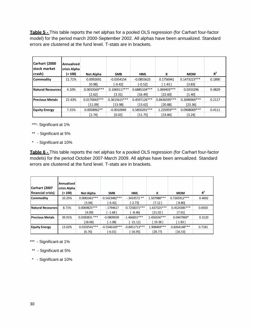
Results shown in Tables 5 indicate that all categories, with the exception of Commodity

funds, have significantly positive alphas during the 2000 stock market crash.9 Precious Metal

9 Note that there were only 2 Commodity funds during this time period. Most of the Commodity funds were

created during 2004/2005 period (According to Morningstar, the first Commodity fund was created in 1997).

15

funds had the best performance with annualized alpha of over 20% (statistically significant at

1%).

[Insert Tables 5]

Performance during the 2007 financial crisis According to the Wall Street Journal, the most recent bear market in US stocks (2007-2009)

was declared in June 2008 after the DJIA had fallen 20% from its October 11, 2007 high. The

bear market reversed course during March, 2009. Our analysis covers of this financial crisis

period from October 2007 to March 2009.

As shown in Tables 6, results support our hypothesis as these funds performed very

well and had significantly positive alphas during the 2007 financial crisis. The Carhart

four-factor model indicates that Commodity funds have an annualized alpha of 10.25%

(statistically significant at 1%). Precious Metals funds had the best performance with

annualized alpha of over 44% (statistically significant at 1%).

[Insert Tables 6]

In summary, the results from both bear market time periods analyzed indicate that, in

general, these funds are an effective hedge during major financial crises generating positive

and significant alphas. The exception being the Commodity funds most of which were

created just before the financial crisis of 2007-2009.10

X. Persistence

10

No benefits of an inflation hedge are evident due to level or declining commodity prices during both periods.

The IMF All Commodity Price Index for the period from March 2000 through September 2002 was basically flat representing no changes in commodity prices over this period. For the period from October 2007 until March 2009, commodity prices declined by approximately 34%.

16

Grinblatt and Titman (1992), Brown et al (1992), Hendricks et al (1993), Brown and Goetzmann

(1994), Goetzmann and Ibbotson (1994), Kahn and Rudd (1995), Malkiel (1995), Elton et al

(1996) and Carhart (1997) have tested the persistence of conventional mutual fund total returns

in time. Grinblatt and Titman (1992) find evidence that differences in performances between

funds persists over time and this persistence is consistent with the ability of fund managers to

earn abnormal returns. Hendricks et al (1993) find that relative performance no-load growth

funds persist in the near term, with the strongest evidence for a one-year horizon. Goetzmann

and Ibbotson (1994) find strong evidence that past mutual fund performance predicts future

mutual fund performance. Their data suggests that winner and losers are likely to repeat, even

when performance is adjusted for relative risk. Kahn and Rudd (1995) investigate performance

persistence for fixed income and equity mutual funds and found performance persistence only

for fixed income funds. However, this persistence edge cannot overcome the average

underperformance of fixed-income funds resulting from fees and expenses. Elton et al (1996)

find that risk-adjusted performances of mutual funds persist, i.e. funds that did well in the past

continue to do well in the future.

Survivorship bias plays a very important role in performance persistence. This impact is

due to truncation of the data set due to disappearance of poorly performing funds from the

sample. Studying only surviving funds will overstate performance. Brown et al. (1992) show

that early studies exaggerate the extent of persistence by relying on survivorship- biased data

sets. Since survivorship bias has been controlled for in our study, there will be no such

problems.

17

Carhart (1997) finds that in his survivorship bias free sample of US equity funds,

persistence disappears after accounting for momentum in stock returns. However, recent

studies argue that after properly considering fund styles, there is persistence in U.S. equity

funds (Ibbotson and Patel (2002); Wermers (2003)).

Following Kahn and Rudd (1995), the following model is used test whether

commodity based mutual funds have any performance persistence.

Period 2 performance is regressed against Period 1 performance. Performance (2) = a + b Χ Performance (1). (10) where ‘Performance’ is annual returns. Positive estimates of coefficient b with significant t-

statistics are evidence of persistence: Period 1 performance contains useful about information

about Period 2 performance.

[Insert Table 7]

Results from Table 7 indicate that none of the categories of commodity based mutual

funds display any performance persistence. Commodities, Natural Resources and Equity Energy

funds have significantly negative persistence, whereas the results are insignificant for Precious

Metals funds.

XI. Mutual fund market-timing & Selectivity

Previous literature (Treynor and Mazuy (1966), Kon and Jen (1979), Henriksson and Merton

(1981), Lee and Rahman (1990)) studies conventional mutual fund market timing and

18

selectivity. They find that mutual fund managers have limited success in market timing and

selectivity.

We use two models to test for market timing and selectivity. The first model was

developed by Treynor and Mazuy (1966). This model adds a quadratic term to CAPM or the

market model to capture market timing and selectivity. The equation is as follows:

Ri,t – Rf,t= αs + β1 (Rm,t - Rf,t) + β2 (Rm,t - Rf,t)2 + e i,t (11)

A positive and significant β2 indicates superior market timing ability. However, a

negative and significant β2 indicates inferior market timing. If β2 is not different than 0,

then the manager has no market timing ability. Similarly, αs measures selectivity.

The second model, which was developed by Henriksson and Merton (1981), replaces

the quadratic term with a variable Max (0, Rm). The equation is as follows:

Ri,t – Rf,t= αs + β1 (Rm,t - Rf,t) + γ[Dt(Rm,t - Rf,t)] + e i,t (12)

Where Dt = 0 if Rm,t > Rf,t (-1 otherwise).

Here, γ measures market-timing ability whereas αs measures selectivity.

[Insert Tables 8a, b, c and d]

As seen in Table 8a, the Treynor and Mazuy (1966) model indicates that Natural

Resources, Precious Metals, and Equity Energy funds exhibit some selectivity, but no market-

timing ability, whereas Commodity funds have neither selectivity nor market-timing ability.

The results of the Henriksson and Merton model are reported in Table 8b. The results for

Commodity, Natural Resource, and Equity Energy funds show no market timing ability and no

selectivity. Precious Metal funds do have selectivity and market timing ability.

19

Following Ferson and Schadt (1996), the conditional market timing and selectivity of

these funds is given by-

Conditional Treynor and Mazuy:

Ri,t – Rf,t= αs + β1 (Rm,t- Rf,t) +δ{zt-1*(Rm,t- Rf,t) }+ β2 (Rm,t- Rf,t)2 + e i,t (13)

Conditional Henriksson and Merton:

Ri,t – Rf,t= αs + β1 (Rm,t- Rf,t) +δ{zt-1*(Rm,t- Rf,t) }+ γ[Dt(Rm,t- Rf,t)] + e i,t (14)

Where Dt = 0 if Rm,t> Rf,t (-1 otherwise).

Conditional Treynor and Mazuy (1966) and Henriksson and Merton (1981) models show

similar results in terms of market timing and selectivity as seen in Tables 8c and d.

XII. Index funds vs. Commodity based mutual funds

Would investors have been better off by investing in index mutual funds or commodity based

funds? Index funds (tracking S&P 500) are passively managed and have lower expense ratios

primarily due to lower management fees. The performance of all index funds tracking the

S&P 500 (living as well as dead) from Inception (September 1976) – December 2012 is

computed. There are a total of 61 index funds tracking S&P 500 during this period. Table 9a

shows the differences in expense ratios and management fees between index funds and

commodity based funds. Index funds have average expense ratio of only 0.65% compared to

1.35% for Commodity, 1.63% for Natural Resources funds, 1.49% for Precious Metals funds;

and 1.60 for Equity Energy funds.

[Insert Tables 9a, b, c, and d]

The performance comparison is made using the Carhart four-factor model and is shown

in Table 9b. For the period starting with the inception of these funds through December

2012, the S&P 500 Index funds had a net annualized alpha that was negative, but better

20

than Natural Resources and Commodities which partially could be explained by the

alternating price (performance) leadership (Zapata, et al., 2012) and/or the relatively low

and stable commodity prices from 1980 through 2000.11

Results in Table 9c and d indicate that the performance of Commodity, Natural

Resources, and Precious Metals and Equity Energy funds was much better than the performance

of Index funds tracking S&P 500 both during the 2000 stock market crash and the 2007 financial

crisis. Based on these results, we conclude that the Commodity (Broad Basket) funds appear to

not provide value as measured by net annualized alpha over long periods of time, but all

categories of commodity based funds provide value during bear markets.

XIII. Conclusions

Our main finding is that investors can benefit by increasing their holdings of these categories of

funds during times of economic distress as evidenced by the 2000 bear market and the 2007

financial crisis. During these bear markets, the net alphas of these funds were significantly

positive and much higher than Index funds tracking S&P 500.

In addition our results indicate that based on the three performance models used in our

study, these categories of funds have not been able to consistently create positive net alphas for

their investors over longer time periods as measured by the time period from their inception

until December 2012. When looking at each category of fund, we find significantly positive

gross alphas for Precious Metals, Natural Resources, and Equity Energy funds, while the gross

alpha of Commodity funds is negative. The results indicate that the funds with positive gross

alphas are successful in finding and implementing new information, however this activity is not

enough to offset the fund expenses as seen by their net alphas. We also observe that Natural

11

See Blake, Bordon and Volz (2013).

21

Resources, Precious Metals funds, and Equity Energy have some selectivity, but no market-

timing ability whereas Commodity funds have neither market-timing nor selectivity.

Based on these results, it is our opinion that during bear markets, there are significant

diversification benefits of these categories of funds relative to the S&P 500 confirming the

rationale as to why investors should hold them in their portfolios as hedges against market

downturns.

22

References

Adams, J. C., Mansi, S. A., & Nishikawa, T. (2009). Internal governance mechanisms and operational

performance: Evidence from index mutual funds. Review of Financial Studies, hhp068.

Aiken, A. L., Clifford, C. P., & Ellis, J. (2012). Out of the dark: Hedge fund reporting biases and

commercial databases. Review of Financial Studies, hhs100.

Aragon, G. O., & Strahan, P. E. (2012). Hedge funds as liquidity providers: Evidence from the Lehman

bankruptcy. Journal of Financial Economics, 103(3), 570-587.

Baks, K. P. (2003). On the performance of mutual fund managers, Working Paper, Emory University.

Barras, L., O. Scaillet, and R. Wermers, 2010, False discoveries in mutual fund performance: Measuring

luck in estimated alphas, The Journal of Finance, 65(1), 179-216.

Bauer, R., K. Koedijk, and R. Otten, 2005, International evidence on ethical mutual fund performance

and investment style, Journal of Banking & Finance, 29(7), 1751-1767.

Bauer, R., R. Otten, and A. Rad, 2006, New Zealand mutual funds: measuring performance and

persistence in performance, Accounting & finance, 46(3), 347-363.

Bauer, R., J. Derwall, and R. Otten, 2007, The ethical mutual fund performance debate: New evidence

from Canada, Journal of Business Ethics, 70(2), 111-124.

Belke, A., Bordon, I. G., & Volz, U. (2013). Effects of global liquidity on commodity and food prices.

World Development, 44, 31-43.

Bhardwaj, G., and A. Dunsby, 2012, The Business cycle and the correlation between stocks and

commodities, Available at SSRN.

Blake, C., E. Elton, and M. Gruber, 1993, The performance of bond mutual funds, Journal of

Business, 66(3), 371-403.

Brown, S. and W. Goetzmann, 1995, Performance persistence, The Journal of Finance, 50(2), 679-

698.

Budiono, D. and M. Martens, 2010, Mutual Funds Selection Based on Funds Characteristics, Journal of

Financial Research, 33(3), 249-265.

Caballero, R., E. Farhi, and P. Gourinchas, 2008, Financial crash, commodity prices and global

imbalances (No. w14521), National Bureau of Economic Research.

Carhart, M., 1997, On persistence in mutual fund performance, The Journal of

Finance, 52(1), 57-82.

23

Christoffersen, S. E., & Sarkissian, S. (2009). City size and fund performance. Journal of Financial Economics, 92(2), 252-275. Columbo, J., The commodities bubble. www.thebubble.com/commodities-bubble. Cremers, K. M., & Petajisto, A. (2009). How active is your fund manager? A new measure that predicts performance. Review of Financial Studies, 22(9), 3329-3365. Davis, J. 2001, Mutual fund performance and manager style. Financial Analysts

Journal, 57(1), 19-27

Detzler M. 1999, The performance of global bond mutual funds, Journal of Banking and Finance, 23(8),

1195-1217.

Elton, E., M. Gruber, and C. Blake,1995, Fundamental economic variables, expected returns, and bond

fund performance, The Journal of Finance, 50(4), 1229–1256.

Gruber, M. J. 1996. Another puzzle: The growth in actively managed mutual funds. The Journal of

Finance, 51(3), 783-810.

Elton, E. J., Gruber, M. J., & Blake, C. R. 1996. Survivor bias and mutual fund performance. Review of Financial Studies, 9(4), 1097-1120. Elton, E., M. Gruber, and C. Blake 1999, Common factors in active and passive portfolios. European

Finance Review, 3(1), 53-78.

Elton, E., M. Gruber, and C. Blake, 2011, Holdings data, security returns and the selection of

superior mutual funds, Journal of Financial and Quantitative Analysis , 46(2), 341.

Fama, E. and K. French, 1993, Common risk factors in the returns on stocks and bonds, Journal of

Financial Economics 33 (1): 3–56

Grinblatt, M. and S.Titman,1992, The persistence of mutual fund performance, The Journal of Finance,

47(5), 1977-1984.

Grossman, S. and J. Stiglitz, 1980, On the impossibility of informationally efficient markets. The

American economic review, 70(3), 393-408.

Gruber, M., 1996, Another puzzle: The growth in actively managed mutual funds. The Journal of

Finance, 51(3), 783-810.

Helbling, T., V. Mercer-Blackman, and K. Cheng, 2012, Commodities in boom, Finance and

Development, 49(2), 30-31.

Henrikkson, R. and R. Merton, 1981, On market timing and investment performance. II. Statistical

procedures for evaluating forecasting skills. The Journal of Business, 54(4), 513-533.

Ippolito, R., 1989, Efficiency with costly information: A study of mutual fund performance, 1965–1984,

Quarterly Journal of Economics, 104(1), 1-23

24

Ippolito, R.,1993, On studies of mutual fund performance, 1962-1991, Financial Analysts Journal, 49(1),

42-50.

Jensen, M., 1968, The performance of mutual funds in the period 1945–1964, The Journal of Finance,

23(2), 389-416.

Kahn, R. N., & Rudd, A. (1995). Does historical performance predict future performance? Financial

Analysts Journal, 61(6), 43-52.

Kon, S. and F. Jen, 1978, Estimation of time varying systematic risk and performance for mutual

fund portfolios: An Application of switching regression, The Journal of Finance, 33(2), 457-475.

Lee, C. F., & Rahman, S. (1990). Market timing, selectivity, and mutual fund performance: an empirical

investigation. Journal of Business, 63(2), 261-278.

López, R., 2009, The great financial crisis, commodity prices and environmental limits, Working Paper,

09-02, University of Maryland, Department of Agricultural and Resource Economics.

Radetzki, M., 2006, The anatomy of three commodity booms, Resources Policy, 31(1), 56-

64.

Schaub, N., & Schmid, M. (2013). Hedge fund liquidity and performance: Evidence from the

financial crisis. Journal of Banking & Finance, 37(3), 671-692.

Sharpe, W.,1964, Capital asset prices: A theory of market equilibrium under conditions of risk,

The Journal of Finance, 19(3), 425-442.

Treynor, J., and Mazuy, K. (1966). Can mutual funds outguess the market. Harvard Business Review,

44(4), 131-136.

Wermers, R., 2000, Mutual fund performance: An empirical decomposition into stock‐picking talent,

style, transactions costs, and expenses, The Journal of Finance, 55(4), 1655-1703.

Wermers, R., T. Yao, and J. Zhao, 2012, Forecasting stock returns through an efficient aggregation of

mutual fund holdings, Review of Financial Studies, 25(12), 3490-3529.

Yan, X., 2006, The determinants and implications of mutual fund cash holdings: Theory and evidence,

Financial Management, 35(2), 67-91.

Yan, X., 2008, Liquidity, investment style, and the relation between fund size and fund performance,

Journal of Financial and Quantitative Analysis, 42(03), 741-767.

Zapata, H., J. Detre, T. Hanabuchi, T., and M. Wetzstein, 2012, Historical Performance of

Commodity and Stock Markets, Journal of Agricultural and Applied Economics, 44(03), 339-357.

25

Appendix 1- Definitions ( Source - Morningstar)

Commodity Broad Basket - portfolios can invest in a diversified basket of commodity goods

including but not limited to grains, minerals, metals, livestock, cotton, oils, sugar, coffee and

cocoa. Investment can be made directly in physical assets or commodity linked derivative

instruments, such as commodity swap agreements.

Natural Resources- Natural resources portfolios focus on commodity-based industries such as

energy, chemicals, minerals, and forest products in the U.S. or outside of the U.S. Some

portfolios invest across this spectrum to offer broad natural resources exposure. Others

concentrate heavily or even exclusively in specific industries including energy or forest products.

Precious Metals- Precious metals portfolios focus on mining stocks, though some do own small

amounts of gold bullion. Most portfolios concentrate on gold-mining stocks, but some have

significant exposure to silver-, platinum-, and base-metal-mining stocks as well. Precious-metals

companies are typically based in North America, Australia, or South Africa.

Equity Energy- Equity Energy portfolios invest primarily in equity securities of U.S. or non-U.S.

companies who conduct business primarily in energy-related industries. This includes and is not

limited to companies in alternative energy, coal, exploration, oil and gas services, pipelines,

natural gas services and refineries.

26

Table 1a

AUM- Assets under management.

All figures in billions of $ (Dec 2012).

The next to last column contains number of funds that died before Dec 2012. Table 1b

Category # of living funds (Dec 2012) AUM (Dec 2012) Dead Funds(Dec 2012) Inception Date (1st fund)

Commodity 30 $50.40 2 Apr-97

Natural Resources 36 $27.90 16 Feb-69

Precious Metals 21 $23.90 9 Mar-56

Equity Energy 34 $26.85 1 Aug-81

Total 121 $129.05 28

Category Mean Standard Deviation Median Max Min

Management fee 0.81 0.24 0.85 1.29 0.30

Commodity Annual Net Expense Ratio 1.35 0.50 1.26 2.75 0.07

Turnover(%) 193.87 440.57 72.50 3455.00 0.00

Management fee 0.85 0.21 0.81 1.35 0.11

Natural Resources Annual Net Expense Ratio 1.63 0.62 1.56 3.84 0.14

Turnover(%) 79.53 60.15 73.00 297.00 7.00

Management fee 0.75 0.19 0.75 1.50 0.26

Precious Metals Annual Net Expense Ratio 1.49 0.53 1.37 3.04 0.29

Turnover(%) 65.25 191.39 22.00 1297.00 1.00

Management fee 0.86 0.24 0.85 1.35 0.12

Equity Energy Annual Net Expense Ratio 1.60 0.54 1.56 2.91 0.14

Turnover(%) 62.66 68.47 43.32 288.00 3.00

27

Table 2a, b, and c- This table reports the net alphas from a pooled OLS regression (for CAPM,

Fama-French three-factor model, and Carhart four-factor model) from Inception-Dec 2012. All

alphas have been annualized. Standard errors are clustered at the fund level. T-stats are in

brackets

***- Significant at 1% ** - Significant at 5%

* - Significant at 10%

CAPM

Annualized

Net Alpha

(× 100) Net Alpha K R2#

Commodity -4.26% -0.0036245*** 0.8304019 *** 0.3419 32

[-3.85] [ 7.63]

Natural Resources 0.60% 0.0005061 1.008464*** 0.4660 52

[1.09] [26.95]

Precious Metals 3.45% 0.0028327 *** 0.5543144 *** 0.0677 30

[4.19] [23.08]

Equity Energy 1.89% 0.0015631** 1.022136*** 0.3899 35

[2.43] [ 21.58]

Fama-French

Annualized

Net Alpha

(× 100) Net Alpha SMB HML K R2#

Commodity -4.14% -0.0035238 *** -0.2612455* -0.1402309 0.9081646*** 0.3512 32

[-3.46] [ -1.90] [-1.13] [ 6.43]

Natural Resources -0.91% -0.0007653 0.1327002*** 0.3726523*** 1.025322*** 0.4922 52

[ -1.65] [ 3.70] [9.79] [30.97]

Precious Metals 2.08% 0.0017202 ** 0.432783 *** 0.2488876 *** 0.525212*** 0.0872 30

[2.55] [16.81] [6.69] [20.02]

Equity Energy 0.68% 0.0005614 0.1188162** 0.3257313*** 1.032103*** 0.4062 35

[0.95] [2.65] [5.87] [26.66]

Carhart

Annualized

Net Alpha

(× 100) Net Alpha SMB HML K MOM R2#

Commodity -4.40% -0.0037494*** -0.2750734** -0.0741139 0.9647944 *** 0.1594232*** 0.3633 32

[-3.82] [-2.08 ] [-0.59] [7.21] [5.58]

Natural Resources -1.05% -0.0008874* 0.1312797*** 0.3794833*** 1.031918*** 0.0188053 0.4924 52

[-1.97] [3.68] [10.26] [33.44] [1.05]

Precious Metals 0.62% 0.000513 0.4257934 *** 0.2983 *** 0.563428**** 0.1449903 *** 0.0918 30

[0.80] [ 16.79] [8.51] [21.11 ] [ 9.16]

Equity Energy 0.007% 6.12e-06 0.1093491 0.3541126*** 1.064608 *** 0.0894793*** 0.4095 35

[ 0.01 ] [2.46] [6.66] [25.25] [4.89]

28

Table 3a, b, and c This table shows the Conditional vs. Unconditional alpha for CAPM, Fama-

French three-factor and Carhart four-factor models from a pooled OLS regression. All alphas

have been annualized. Standard errors are clustered at the fund level. T-stats are in brackets.

***- Significant at 1% ** - Significant at 5%

* - Significant at 10%

CAPM

Annualized

Alpha (× 100)

Unconditional

net alpha R2

Annualized

Alpha (× 100)

Conditional net

Alpha R2

Commodity -4.26% -0.0036245*** 0.3419 -4.54% -0.0038682 *** 0.3592

[-3.85] [-4.00]

Natural Resources 0.60% 0.0005061 0.4660 0.104% 0.0000873 0.4799

[1.09] [0.20]

Precious Metals 3.45% 0.0028327 *** 0.0677 3.86% 0.0031636*** 0.0725

[4.19] [ 4.94]

Equity Energy 1.89% 0.0015631** 0.3899 2.44% 0.0020149*** 0.4048

[2.43] [2.98]

Fama-French

Annualized

Alpha (× 100)

Unconditional

net alpha R2

Annualized

Alpha (× 100)

Conditional net

Alpha R2

Commodity -4.14% -0.0035238 *** 0.3512 -4.48% -0.0038181*** 0.3763

[-3.46] [ -3.53 ]

Natural Resources -0.91% -0.0007653 0.4922 -1.21% -0.0010146 0.4953

[ -1.65] [-1.67]

Precious Metals 2.08% 0.0017202 ** 0.0872 2.25% 0.0018549*** 0.0926

[2.55] [2.77]

Equity Energy 0.68% 0.0005614 0.4062 1.17% 0.0009657 0.4166

[0.95] [1.63]

Carhart

Annualized

Alpha (× 100)

Unconditional

net alpha R2

Annualized

Alpha (× 100)

Conditional net

Alpha R2

Commodity -4.40% -0.0037494*** 0.3633 -4.99% -0.0042597*** 0.3929

[-3.82] [ -3.91]

Natural Resources -1.05% -0.0008874* 0.4924 -1.37% -0.0011469 *** 0.4956

[-1.97] [ -2.74]

Precious Metals 0.62% 0.000513 0.0918 0.77% 0.0006434 0.0983

[0.80] [1.01]

Equity Energy 0.007% 6.12e-06 0.4095 0.60% 0.000506 0.4198

[ 0.01 ] [0.89]

29

Table 4a, b and c- This table reports the gross alphas from a pooled OLS regression (for CAPM, Fama-French three-factor model, and Carhart four-factor models) from Inception-Dec 2012. All alphas have been annualized. Standard errors are clustered at the fund level. T-stats are in brackets

*** - Significant at 1% **- Significant at 5%

* - Significant at 10%

CAPM

Annualized

Gross Alpha

(× 100) Gross Alpha K R2

Commodity -3.04% -0.002568 *** 0.8312145 *** 0.3419

[-2.85] [ 7.63]

Natural Resources 1.97% 0.0016283 ** 0.4209685*** 0.1189

[ 2.65 ] [ 4.15]

Precious Metals 5.06% 0.0041218 *** 0.5568964*** 0.0680

[ 5.76] [ 25.77]

Equity Energy 3.46% 0.0028399*** 1.023539*** 0.3900

[4.39] [21.56]

Fama-French

Annualized

Gross Alpha

(× 100) Gross Alpha SMB HML K R2

Commodity -2.92% -0.0024673** -0.2614783* -0.1405568 0.9090726*** 0.3511

[ -2.51 ] [-1.90] [-1.13] [6.43]

Natural Resources 1.40% 0.0011604 * 0.0210269 0.146045*** 0.4333718 *** 0.1247

[1.77 ] [0.75] [ 3.33] [ 4.22]

Precious Metals 3.67% 0.0030091*** 0.4456573*** 0.251161*** 0.5278918*** 0.0884

[4.51] [ 18.11] [ 7.08] [ 21.88]

Equity Energy 2.23% 0.0018367 *** 0.1191829** 0.3261339*** 1.033476*** 0.4063

[3.06] [2.65] [5.87] [26.64]

Carhart

Annualized

Gross Alpha

(× 100) Gross Alpha SMB HML K MOM R2

Commodity -3.18% - 0.0026931*** -0.2753193** -0.0743772 0.965756*** 0.1595741*** 0.3633

[-2.87] [-2.08] [ -0.59] [7.21] [5.56]

Natural Resources 1.51% 0.0012502 * 0.0220716 0.1410192*** 0.4285187*** -0.0138354 0.1249

[ 1.89] [0.78] [3.29] [ 4.11 ] [-0.71]

Precious Metals 2.11% 0.0017437** 0.438632 *** 0.3025232*** 0.5664114*** 0.1498341*** 0.0933

[ 2.80] [17.93] [ 9.09] [23.65] [ 10.39]

Equity Energy 1.55% 0.0012799** 0.10969** 0.3545925*** 1.06607*** 0.089723*** 0.4096

[2.32] [2.46] [6.67] [25.23] [4.90]

30

Table 5 - This table reports the net alphas for a pooled OLS regression (for Carhart four-factor

model) for the period march 2000-September 2002. All alphas have been annualized. Standard

errors are clustered at the fund level. T-stats are in brackets.

***- Significant at 1%

** - Significant at 5%

* - Significant at 10%

Table 6 - This table reports the net alphas for a pooled OLS regression (for Carhart four-factor

models) for the period October 2007-March 2009. All alphas have been annualized. Standard

errors are clustered at the fund level. T-stats are in brackets.

*** - Significant at 1% ** - Significant at 5%

* - Significant at 10%

Carhart (2000

stock market

crash)

Annualized

crisis Alpha

(× 100) Net Alpha SMB HML K MOM R2

Commodity 11.71% 0.0092691 -0.0354154 -0.0855625 0.1756941 0.1473223*** 0.1890

[0.98] [-0.42] [-0.52] [ 1.43 ] [3.83]

Natural Resources 4.10% 0.0033569*** 0.1069117*** 0.6885104*** 1.069403*** 0.0333296 0.4829

[2.62] [3.31] [16.49] [22.60] [1.40]

Precious Metals 22.43% 0.0170043*** 0.3615615*** 0.4597126*** 0.8436595*** 0.2696969*** 0.2117

[11.09] [13.98] [13.62] [20.88] [23.36]

Equity Energy 7.31% 0.0058962** -0.0010949 0.5850291*** 1.235959*** 0.0908009*** 0.4111

[2.74] [0.02] [11.75] [23.84] [3.24]

Carhart (2007

financial crisis)

Annualized

crisis Alpha

(× 100) Net Alpha SMB HML K MOM R2

Commodity 10.25% 0.0081661*** -0.5423482*** -.3433572 ** 1.507988*** 0.7265912*** 0.4692

[3.04] [-6.42] [-2.73] [7.12 ] [ 8.80]

Natural Resources 8.71% 0.0069825*** -.1794617 -0.7258371*** 1.637325*** 0.4524385*** 0.6920

[4.09] [ -1.68 ] [ -8.46] [21.02 ] [7.01]

Precious Metals 39.91% 0.0283831 *** -0.0809039 -1.466831*** 1.456556*** 0.0447969* 0.3120

[18.06] [-1.08] [ -21.11] [ 19.38 ] [ 1.83 ]

Equity Energy 13.02% 0.0102541*** -0.5546169*** -0.8451713*** 1.908469*** 0.8264148*** 0.7181

[6.76] [-6.01] [-16.95] [28.77] [16.53]

31

Table 7- Reported are the results of Kahn and Rudd (1995) performance persistence model. Standard errors are clustered at the fund level. T-stats are in brackets. Period 2 performance is regressed against Period 1 performance. Performance (2) = a + b Χ Performance (1). where ‘Performance’ is annual returns. Positive estimates of coefficient b with significant t- statistics are evidence of persistence: Period 1 performance contains useful information about Period 2 performance.

***- Significant at 1% ** - Significant at 5%

* - Significant at 10%

Kahn and Rudd (1995) a b R2

Commodity 0.0527178** -0.3692058*** 0.1606

[2.17 ] [ -10.54 ]

Natural Resources 0.142861*** -0.2668571*** 0.0757

[17.53 ] [-9.31]

Precious Metals 0.1024856*** 0.0369648 0.0014

[ 7.93] [1.51 ]

Equity Energy 0.1546694*** -0.2370113*** 0.0604

[12.54] [-6.78]

32

Table 8a, b, c, and d- Reported are the results from Treynor and Mazuy (1966), Henriksson and

Merton (1984) and conditional Treynor and Mazuy and Henriksson and Merton models. For the

Treynor and Mazuy (1996) models, αs measures selectivity whereas β2 measures market-

timing. Similarly, for the Henriksson and Merton (1984) models, αs measures selectivity

whereas γ measures market-timing. Standard errors are clustered at the fund level. T-stats are

in brackets.

Treynor and Mazuy αs β2 R2

Commodity 0.0011606 -1.947379 *** 0.3536

[ 0.80 ] [ -4.54 ]

Natural Resources 0.0021186*** -0.6827301*** 0.4674

[3.06] [-3.89]

Precious Metals 0.0092401*** -2.875043*** 0.0807

[9.83] [-9.54]

Equity Energy 0.0049938*** -1.501977*** 0.3953

[8.12] [-8.40]

Henriksson and Merton αs γ R2

Commodity -0.0072827*** -0.0085214* 0.3434

[ -3.99] [-1.87]

Natural Resources -0.0005612 -0.00246 0.4661

[-0.56] [-1.44 ]

Precious Metals 0.0050555 *** 0.0050565* 0.0679

[3.77] [2.01]

Equity Energy 0.0023185 0.001746 0.3900

[1.54] [0.73]

33

***- Significant at 1% ** - Significant at 5%

* - Significant at 10%

Conditional Treynor

and Mazuy αs β2 R2

Commodity 0.0021522 -2.860844*** 0.3800

[1.43] [-6.80]

Natural Resources 0.0023877*** -1.009675*** 0.4830

[3.41 ] [-5.55]

Precious Metals 0.0092401*** -2.875043*** 0.0807

[9.83] [-9.54]

Equity Energy 0.0055106*** -1.637158*** 0.4107

[8.90] [-8.04]

Conditional

Henriksson and

Merton αs γ R2

Commodity -0.0065639*** -0.0062493* 0.3600

[-4.86] [-2.01]

Natural Resources -0.0004482 -0.0012197 0.4800

[-0.45] [-0.71]

Precious Metals 0.0050555 *** 0.0050565* 0.0679

[3.77] [2.01]

Equity Energy 0.0035578** 0.0035154 0.4050

[ 2.30 ] [ 1.44]

34

Table 9a- Expenses and turnover for index funds tracking S&P 500 and Commodity, Natural

Resources, Precious Metals, and Equity Energy mutual funds.

Comparision Number Mean Standard Deviation Median

Management fee 0.20 0.16 0.18

Index Mutual Funds 61 Annual Net Expense Ratio 0.65 0.47 0.57

Turnover(%) 9.89 24.60 5.00

Management fee 0.81 0.24 0.85

Commodity 32 Annual Net Expense Ratio 1.35 0.50 1.26

Turnover(%) 193.87 440.57 72.50

Management fee 1.35 0.21 0.81

Natural Resources 52 Annual Net Expense Ratio 1.63 0.62 1.56

Turnover(%) 79.53 60.15 73.00

Management fee 0.75 0.19 0.75

Precious Metals 30 Annual Net Expense Ratio 1.49 0.53 1.37

Turnover(%) 65.25 191.39 22.00

Management fee 0.86 0.24 0.85

Equity Energy 35 Annual Net Expense Ratio 1.60 0.54 1.56

Turnover(%) 62.66 68.47 43.32

35

Table 9b show the difference in performance between passively managed index mutual funds

tracking S&P 500 and Commodity, Natural Resources, Precious Metals, and Equity Energy

mutual funds (using alpha from Carhart four-factor model) from inception-Dec 2012. All alphas

have been annualized. Standard errors are clustered at the fund level. T-stats are in brackets.

***- Significant at 1% ** - Significant at 5%

* - Significant at 10%

Carhart (Inception-

Dec 2012)

Annualized

net Alpha

(× 100) Net Alpha R2

Index Funds (S&P 500) -0.32% -0.0002698 *** 0.9716

[ -4.02 ]

Commodity -4.40% -0.0037494*** 0.3633

[-3.82]

Natural Resources -1.05% -0.0008874* 0.4924

[-1.97]

Precious Metals 0.62% 0.000513 0.0918

[0.80]

Equity Energy 0.007% 6.12e-06 0.4095

[ 0.01 ]

36

Tables 9c and d show the difference in performance between passively managed index mutual

funds tracking S&P 500 and Commodity, Natural Resources, Precious Metals and Equity

Energy mutual funds (using alpha from Carhart four-factor model) during the 2000 stock market

crash (March 2000 – September 2002) and the 2007 financial crisis (October 2007 – March

2009). All alphas have been annualized. Standard errors are clustered at the fund level. T-stats

are in brackets.

***- Significant at 1%

** - Significant at 5%

* - Significant at 10%

Carhart (March 2000

- September 2002)

Annualized

crisis Alpha

(× 100)

Net Alpha

(crisis) R2

Index Funds (S&P 500) -0.45% -0.0003755** 0.9437

[-2.33]

Commodity 11.71% 0.0092691 0.1890

[0.98]

Natural Resources 4.10% 0.0033569*** 0.4829

[2.62]

Precious Metals 22.43% 0.0170043*** 0.2117

[11.09]

Equity Energy 7.31% 0.0058962** 0.4111

[2.74]

Carhart (Oct 2007 -

March 2009)

Annualized

crisis Alpha

(× 100)

Net Alpha

(crisis) R2

Index Funds (S&P 500) -1.243% -0.0010419*** 0.9979

[-12.15]

Commodity 10.25% 0.0081661*** 0.4692

[3.04]

Natural Resources 8.71% 0.0069825*** 0.6920

[4.09]

Precious Metals 39.91% 0.0283831 *** 0.3120

[18.06]

Equity Energy 13.02% 0.0102541*** 0.7181

[6.76]