Commodity Index Funds: The price impact of the rollon commodities futures contracts

Loıc Marechal∗

April 15, 2019

Abstract

We identify and date two significant breaks, previously only backed by anecdotal orvisual evidence: i) one in index fund investment and ii) one in the amount of arbitragecapital. To see whether these changes in investors’ clientele had an impact on com-modity futures prices, we conduct an event study based on several benchmarks. TheCASRs (cumulated abnormal spreading returns) of individual contracts are 17 basispoints at most -the order of magnitude of minimum possible transaction costs- andare never statistically significant when we adjust the standard errors for event-inducedcross-correlation and variance. The test hypotheses of hedging induced price pressure,sunshine trading and predatory trading yields mixed and mostly insignificant results.

JEL classification: G24, G28, K22, K42.

Keywords : Commodity index investment, predatory trading, price pressure, hedging pres-sure, sunshine trading.

∗University of Neuchatel, loic.marechal@unine.ch

1. Introduction

Academic research shows that investing in commodities futures improves portfolio diversi-

fication (Bodie and Rosansky, 1980), as commodities display anti-cyclical behaviour (Gorton

and Rouwenhorst, 2006), represent a hedge against inflation (Greer, 2000), are negatively

correlated with the US Dollar (Rezitis, 2015). Moreover, their price change distribution is

positively skewed (Deaton and Laroque, 1992).1 These characteristics make this asset class

particularly attractive. However, a direct investment in commodities is not easily achievable.

In particular, long-term holdings are difficult to maintain because of the physical nature of

the underlying (storage costs, decay, logistics). The major investment products that per-

mit exposure to commodities are Exchange Traded Funds (ETFs), Exchange Traded Notes

(ETNs), and mutual funds tracking long only indices. These indices are composed of various

commodity futures contracts with different allocation.

Indeed, the primary focus of index investment is to obtain an exposure to commodities.

These products replicate a specific index through long positions in the nearest to maturity

(hereafter nearby) futures contracts to minimize the term-structure effects and maximize the

liquidity. Hence these indices roll their positions at fixed time intervals before the underlying

futures contracts mature. The products that replicate these indices represent a significant

part of the long open interest (OI) of commodity futures. Because every position of these

products is fully rebalanced before the maturity of the corresponding contracts, there are

suspicions that such investments distort the market. In several news articles,2 Dizard (2007)

points out that the beneficiaries of the “congestion roll trade” or “date rape” are speculators

on the floors of commodities exchanges or, more likely, the banks selling securities based on

these indices. In a public hearing before the US Senate, Masters (2008) declared that “Index

speculators have driven futures and spot prices higher”. To support his view, he shows that

the proportion of traditional speculators has been overtaken by that of index speculators.

He also insists on the fact that index speculators’ demand is unrelated to the supply and

demand of the underlying commodities.

In this paper, we examine whether the changes of market participation induced by com-

modity indices traders (CITs), also called the “financialization” of commodities markets, has

a material effect on commodity futures prices at the date the index rolls positions from the

nearby to the second nearest (hereafter first deferred) contract. To address these questions,

1For an exhaustive review of these stylized facts, see also Gorton and Rouwenhorst (2006) and Erb andHarvey (2006).

2“Speculators profit from commodity investors”, Financial Times, January 22, 2007. See also, “GoldmanSachs and its magic commodities box”, Financial Times, February 5, 2007, and “U.S. oil fund finds itself atthe mercy of traders”, Wall Street Journal, March 6, 2009.

1

we focus on the constituents of the Standard and Poor’s Goldman Sachs Commodity Index

(SP-GSCI).3

The financialization should translate into a significant change in OI of the contracts

included in the SP-GSCI and more specifically in the proportion of OI resulting from the

“Managed Money” sub-category.4 However, there is no official date for this change in market

participation. Therefore, we check empirically for a structural change in index investment

share of total OI over the period from 1992 to 2017. We find this change to occur in

August 2003, about half a year before the dates used in Boons, Roon de, and Szymanowska

(2014), and five years before the breaks identified on the Crude Oil futures returns series by

Hamilton and Wu (2015). Academic studies also mention the sudden increase of arbitrage

capital, approximated by the amount of spreading positions held by speculators, following

the financialization. Hence, we also examine, over the same period, the ratio of spreading

positions over total OI. A high value of this ratio should ease the index investors’ activity

during the roll. We find a break in August 2005 for this series.

If the financialization has a permanent effect on commodity futures markets, it should be

visible when funds rebalance their positions from the nearby to the first deferred contract.

The SP-GSCI rolls its position from the fifth to the ninth business day of the month preceding

maturity. Every day, the index transfers 20% of its positions from one contract to the next.5

We focus on this particular roll window, because it overlaps most of the other windows of first

generation indices such as the BCOM or the procedure of US funds on diversified and single

commodities. We analyze the spreading returns during the roll, and estimate the valuation

effect of the financialization of commodity markets with an event-study. As a counterfactual

of futures returns, we use several benchmarks that give consistent empirical results. We also

control for event clustering as thirteen over twenty seven constituents of the SP-GSCI roll

every month.

We confirm that, with no correction for event-induced variance and cross-correlation,

the average cumulative spreading returns are positive (0.10 bp during the roll, 0.17 bp in

3The three major diversified indices in terms of tracking OI are the SP-GSCI, the Bloomberg CommodityIndex (BCOM), formerly Dow Jones UBS Commodity Index (DJ-UBSCI) and the Deutsche Bank Commod-ity Index (DBCI). Other diversified indices exist, such as the Reuters-Jefferies CRB Index (RJ-CRB), theRogers International Commodity Index (RICI), the Chase Physical Commodity Index, Pimco, Oppenheimeror Bear Sterns. Other non-diversified funds directly track subsectors (energy, agricultural futures) or singlefutures (crude oil, natural gas, gold).

4We focus on the SP-GSCI contracts in our setting but impute the value for the total index investmenttargeting these contracts, that follows closely the SP-GSCI methodology and roll.

5The roll procedure is the same for every contract, which creates a distortion in the actual time tomaturity during the roll. The last notice day of the sugar NY#11 contract on NYMEX for instance is thelast business day of the preceding month, while the grains contracts traded on the CME are generally the15th business day of the maturity month.

2

the pre-roll window), and statistically significant at the 1% level up until 2003. However,

once we correct for clustering, the significance disappears. When we consider individual

futures contracts, we find that cumulative abnormal spreading returns (CASRs) are not

statistically significant in any period and even before adjustement. In addition, previous

studies documenting significant abnormal returns around the roll do not take into account

the substantial transaction costs associated with such strategies; see, e.g., Mou (2011). We

evaluate these transaction costs, and find that they are as high as the abnormal returns

themselves. In brief, we find that the residual profit left by arbitragers is of the size of

their potential transaction costs, would they enter the trade. Finally, while Bessembinder,

Carrion, Tuttle, and Venkataram (2016) find that the roll of a major oil ETF on a single

day does not affect significantly futures prices, we extend their results to the roll of the SP-

GSCI constituents. Our results contribute to the view that index investment has not been

detrimental for the functioning of the commodity futures markets themselves. However,

our results do not discard the possibility of intraday predatory trading achieved by funds

managers ahead of their hedging trades, which penalizes the funds and ETFs performance.

The remainder of the paper is organized as follows. Section 2 presents the hypothe-

sis development with respect to the existing literature. Section 3 provides details on the

methodology and the sample construction. Section 4 presents the main results and discusses

their robustness. Section 5 shows additional findings using the futures contract written on

the SP-GSCI and Section 6 concludes.

2. Prior literature and hypothesis development

Following Master’s hearing before the US Senate, a series of papers examine whether the

financialization of commodity futures affects commodity prices. In their survey, Cheng and

Xiong (2014) list the consequences of this structural break: the increase of price pressure

phenomena, the effects on risk sharing between hedgers and speculators, and the distortion

of stock prices resulting from speculation. The scope of this section is more limited since we

examine how this change should materialize, and what are the potential effects of the roll

on futures prices.

2.1. Price pressure and hedging pressure

Grossman and Miller (1988) present a three period model in which there are two types of

agents, market makers and outside customers. They derive the demand function assuming

that prices are normally distributed, and investors maximize their expected (exponential)

3

utility. In their setting, they analyze the consequences of a liquidity shock that creates

a temporary order imbalance, and show how market makers are compensated for bearing

the risk during the holding period. They show that the (absolute) expected returns are an

increasing function of the order imbalance, and an inverse function of the number of market

makers. In our case, assuming that the market cannot absorb instantaneously the positive

demand (supply) shock on the first deferred (nearby) contract, we should observe an increase

(decrease) in the current price.

Brunetti and Reiffen (2014) derive a two period model where CITs’ demand is exogenous,

and additional assumptions similar to those of Grossman and Miller (1988). There are

two types of agents (hedgers and speculators) in the model that maximize their expected

(exponential) utility. Under the assumption of normal futures prices, they derive the demand

for futures positions. A comparative statistics shows that, as index traders roll their positions

from the nearby to the first deferred contract, the spread between the futures prices widen.

More specifically, the price of the nearby contract decreases (lower demand) while the price of

the first deferred contract increases (higher demand). Their empirical results are consistent

with this prediction. In addition, Aulerich, Irwin, and Garcia (2013) find a significant

association for the index traders’ position roll with the returns on the two legs of the spread

but of opposite directions. That is, the return on the nearby contract increases when the

index traders unwind their position, whereas the price of the first deferred contract decreases

as index traders build their new position.

Henderson, Pearson, and Wang (2015) examine the impact of the flows of financial in-

vestors on commodity futures prices through commodity-linked notes (CLNs). These flows,

generated by CLN issuers hedging their liabilities on the commodities futures markets, are

also not based on information about futures price movements. Nevertheless, they cause

increases (buy pressure) and decreases (sell pressure) in commodity futures prices. These

results are consistent with Bessembinder et al. (2016) who study the roll from the nearby to

the first deferred contract of the United States Oil Fund (USO), a large fund invested solely

in WTI crude oil futures contracts. They show that accumulated trading costs resulting

from this price pressure amounts to 3% per year.

Roon de, Nijman, and Veld (2000) propose a model for futures expected returns with

three types of assets, two of which are marketable (financial securities and futures positions),

and one is not. In a mean variance framework, they show that, beyond the market risk

premium, own hedging and cross hedging pressures are priced. These results are confirmed

empirically, and remain after controlling for price pressure measured by the change in own

hedging pressure.

4

2.2. Non-informative trades and the sunshine trading hypothesis

The roll policy of commodity index funds (ETFs, ETNs, and mutual funds) is mentioned

in their prospectus, and generally similar to that of the index they replicate. For the SP-

GSCI futures, the roll period applies every month for 13 commodities, and every two, three

or more months for the remaining 14 commodities.6 The amounts involved in the rolling are

also easy to estimate for the funds that strictly follow the index roll policy since the assets

under management (AuM) are known. Therefore, most of the trades related to the rolling

are initiated by known investors, of known size, and do not contain information that is not

already known by market participants.7

Admati and Pfleiderer (1991) develop a model where some liquidity traders preannounce

the size of their orders. These preannouncements are initiated with the goal to reduce

the price impact of the trade. The preannouncement changes the nature of informational

asymmetries in the market, in particular when trades are not related to information. The

trading costs of traders that preannounce their trades are reduced, but the effect on other

traders is ambiguous (trading cost and welfare). This practice, known as “sunshine trading”,

is of particular interest to us because it shares many commonalities with the commodity index

funds roll. However, index fund managers neither explicitly announce their trades, nor the

intraday timing within the window.

2.3. Predatory trading

Brunnermeier and Pedersen (2005) study a distressed trader, a distressed hedge fund

for example, who reveals some information to predatory traders (e.g., its broker dealer).

In their setting, the predatory trader is aware of the trader’s needs to liquidate quickly her

positions. The model foresees a higher price impact as the predator trades on this information

along or before the distressed trader. Hence, the liquidation value of the distressed fund

decreases. The model also features long-term investors who do not have this information or

the willingness to initiate such predatory trades. It predicts that the more predatory traders

compete, the lower the (permanent) price impact. With an infinity of predatory traders,

the effect is similar to the one of price pressure alone. In our setting, we assume the entire

market to know about the trades, and thus, to be in this corner case.

6See the contract description in appendix C.7At first glance, the roll looks very much like stock index inclusion (first deferred contract) and deletion

(nearby contract). However, there are two notable differences. First, changes in stock index composition areless frequent (20 per year on average for the S&P 500) than changes in the SP-GSCI index (more than 250per year). Second, the index is built on stocks (positive net supply), and not on futures contracts (zero netsupply).

5

From an empirical perspective, Mou (2011) explores the performance of a strategy that

front runs the SP-GSCI official roll by five and ten days from 1980 to 2009. Both strategies

take a long position in the second nearby contract and a short position in the first nearby con-

tract. These strategies generate abnormal returns beyond that of the SP-GSCI constituents

after controlling for the average roll yield of commodities, GDP growth, and inflation. For

non SP-GSCI constituents, there is no abnormal returns. He argues that transaction costs

are very low, and estimates them to the minimum possible fluctuation of one percentage

in point (pip). The best performing strategy that takes positions ten days ahead the roll

delivers an average monthly 31 bp per roll before transaction costs from 2000 to 2010. He

attributes these findings to the limits of arbitrage capital leading to price pressure. Under

these conditions, there is also potential room for front trading. Additionally, he shows that

abnormal returns are positive and related to the ratio of index investment and arbitrage

capital. Finally, he estimates the costs of this lack of arbitrage to USD 8.4 billion in 2009,

for a total index investment of USD 211 billion.

Bessembinder et al. (2016) re-examine theoretically the predatory trading hypothesis by

considering that the price impact of trades has both a transitory and a permanent component.

In this setting, they demonstrate that a monopolistic predator benefits a sunshine trader if

the permanent component is not very large, and if the transitory component vanishes quickly.

They study empirically the roll of the USO, which takes place at a known date. They show

that more individual trading accounts provide liquidity on roll date, and find no systematic

use of predatory strategies. To summarize, their results are consistent with the sunshine

trading hypothesis.

3. Methodology and hypotheses

3.1. Dating the financialization

Masters (2008) shows that the proportion of OI from CITs (IND) changed dramatically

from 1998 to 2008, which makes this ratio a natural candidate to look for a potential break

caused by index investors. As a result of the financialization, we should observe a common

break affecting simultaneously the IND for the futures contracts constituents of the SP-

GSCI index. Therefore, our first hypotheses set is as follows:

H1a: IND of commodities futures contracts constituents of the SP-GSCI show a com-

mon break during the 1992 – 2017 period.

6

A related question is whether there is enough arbitrage capital to offset the price pres-

sure of CITs’ roll. Following the literature (see, e.g., Stoll and Whaley, 2010 and Irwin and

Sanders, 2012), we define the ratio of spreading positions over total OI as a proxy for the

arbitrage capital deployed by speculators to ease the index investors’ activity during the roll

(or profit from it). We check for a common break affecting the constituents of the SP-GSCI

index.

H1b: Ratios of arbitrage capital over total OI (ARB) on commodity futures contracts

constituents of the SP-GSCI show a common break during the 1992 – 2017 period.

Since 1986, the “Commitment of Traders” (COT) reports on a weekly basis the long and

short positions of the “commercial category”, and the long, short and spreading positions

of the “non-commercial category” for every US futures contract (that has at least 20 active

trader positions above a threshold defined by the CFTC for each contract). In 2006, the

CFTC revised these categories, and added the “supplemental” and “disaggregated” reports.8

The disaggregated report splits the original categories of commercial and non-commercial

traders, in hedgers,9 swap dealers, managed money, and other reportable. The supplemental

report refers to 13 agricultural futures contracts, and adds a CIT category that aggregates

all the positions reported in the above mentioned categories and that are managed for com-

modity investment vehicles, ETFs, ETNs and funds. We download the COT report data

from the CFTC website10 and compute the variable IND, ARB and others, for the SP-GSCI

futures contracts.

To compute the numerator of IND, we use the information of Masters and White (2008),

the CFTC CIT report, the total OI, the SP-GSCI weights, the underlying quantities and

the prices. We then apply the Masters’ algorithm (see, e.g., Masters, 2008; Mou, 2011 and

Sanders and Irwin, 201311). We describe the procedure in the appendix A. In Figure 1, we

plot the monthly SP-GSCI investment, total arbitrage capital, total OI and total trading

8The CFTC disaggregated the positions because of the classifications of most of the swap dealers intothe commercial category. Despite their role is non-speculative, they dedicate a large part of their activity tohedge indices related position. In addition, for the same reasons, they could claim the exchanges for positionlimits exemptions, as if they were producers in needs of hedging.

9The official CFTC classification is Producer/Merchant/Processor/User.10http://www.cftc.gov/MarketReports/CommitmentsofTraders/index.htm11Sanders and Irwin (2013), argue that the Masters algorithm produces index investment figures that are

sensitive to the low weighted contracts generally used to impute the overall index investment. In particularthey find the correlation between index investment figures of the CFTC and the Masters algorithm to beextremely low and sometimes negative. Instead, we find that the lowest correlation is 0.62 for the KansasWheat contract and that all other coefficients are above 0.77. Moreover the index investment values lie in aclose range.

7

volume, for the 27 selected contracts12 and expressed in USD.

[Insert Figure 1 here]

We look for a break in the commodity futures contracts open interest ratios, IND and

ARB, using the Bai, Lumsdaine, and Stock (1998) algorithm. We estimate a V AR(1), and

restrict the break to apply to the intercept only. The estimated equation is,

yt = (G′t ⊗Gt) θ + dt (k) (G′t ⊗ In)S ′Sδ + εt, (1)

where yt is the stack vector of IND or ARB series, G′t is a row vector containing yt−1

and a constant, n is the number of equations, and S is a selection matrix such that only the

intercept is allowed to break with S = s⊗ In and s = (1, 0, ..., 0). We estimate the system of

equations for every potential breaking date k, such that dt (k) = 0 for t ≤ k and dt (k) = 1

for t > k. We identify the break date as the value of k that generates a maximum Wald

statistic higher than the limiting χ2 distribution. Then, we construct the confidence interval

(in days) of the estimated break date k, for a given level of statistical significance.

3.2. The valuation effect of the roll

We revisit the valuation effect of the financialization of commodity markets during the

rolling period for several reasons. First, previous research use an ad hoc date to determine

when financialization is supposed to materialize. Alternatively, we estimate the potential

structural change through a statistical method, which is less arbitrary. Second, while the

benchmarks in event studies based on stock returns are well established, there is no consen-

sus on how to compute abnormal spreading returns in the existing literature. Mou (2011)

does not adjust the CASRs directly, while Henderson et al. (2015) use a linear factor model

for returns on single futures contracts. The period over which abnormal returns could ma-

terialize is not well identified. Depending on the scenario, abnormal returns are supposed to

occur before or during the rolling period. Third, every month, between 16 and 24 futures

commodity contracts are rolled. The residual terms, i.e. the error in the estimation win-

dow and the CASRs during the event window, could be cross-correlated because of missing

variables in the benchmark model. Ignoring this cross-correlation shrinks the standard error

of the CASRs, which in turns leads to an over-rejection of the null hypothesis (abnormal

returns are too frequently different from zero).

12Except for the London Metal Exchange (LME) contracts, not covered by the CFTC and for which thespreading positions of speculators is not available.

8

We test the valuation effect on spreading returns for two reasons. First, during a roll,

an index fund sells and buys the same quantity on both legs. Thus, we expect a magnified

effect when looking at both contracts simultaneously. Second, spreading returns avoid the

concurrent effect of fundamental shocks that may shift the whole term structure at once.

We also examine the valuation effect on both the nearby and first deferred contracts. The

reason is that the market reaction could be different on both legs. Therefore, we set our

second hypothesis as follows:

H2a: Abnormal spreading returns (returns on the first deferred minus nearby contract)

on SP-GSCI contracts are null during the SP-GSCI roll periods from 1992 to 2017 and during

the sub-periods.

H2b: Abnormal returns on the nearby and first deferred contracts constituents of SP-

GSCI are null during the roll periods from 1992 to 2017 and during the sub-periods.

H3a: Abnormal spreading returns are null during the week preceding the SP-GSCI roll

periods from 1992 to 2017 and during the sub-periods.

H3b: Abnormal returns on the nearby and first deferred contracts are null during the

week preceding the roll periods from 1992 to 2017 and during the sub-periods.

To test the aforementioned hypotheses, we conduct an event-study. First we download

the daily closing prices of the 27 commodity futures constituents of the SP-GSCI for the first

five consecutive maturities m. The sample starts on January 2, 1992 and ends on September

22, 2017. We compute the daily arithmetic futures returns for every maturity available as

Rmc,t =

Fmc,t

Fmc,t−1− 1, when no expiry occurs between t− 1 and t and Rm

c,t =Fmc,t

Fm+1c,t−1

− 1 otherwise.

Fmc,t is the futures price of commodity c, on day t and for each maturity.13 We define the

spreading returns as SRmc,t = Rm+1

c,t −Rmc,t, for every maturity of the term structure.14 Finally,

we download and compute the returns on the MSCI emerging market index, SP-500 index,

USD index, VIX, T-Bond, Baltic Dry Index, and inflation indices; see Henderson et al. (2015).

We download the data from Thomson Reuters and the Commodity Research Bureau.

First, we estimate the valuation effect of the roll with an event study that relies on a

parametric benchmark for both spreading and individual returns, and account for cross cor-

13There are expiry dates variations across the contracts, with maturity standing at the beginning or endof the quoted months. Other contracts matures during the month preceding their quoted months.

14Although it is only fully numerically true for log returns, the standard deviation is so small that we areconfident to use this approximate raw-log equality.

9

relation of commodity returns during the window; see Kolari and Pynnonen (2010). The

counterfactual (benchmark) of the nearby spreading returns is a linear function of the spread-

ing returns based on further to maturity contracts (see the appendix B). We estimate the

abnormal spreading returns during the roll as a Seemingly Unrelated Regression (SUR; see

Zellner, 1962) with a single pass estimation,15,16

SR1c,t = α0,c + CASRc,e ×∆roll

c,t + α1,c × SR3c,t + εc,t, (2)

where c is the commodity contract, t is the current time, ∆rollc,t is an individual commod-

ity dummy vector equal to 0.2 for every day of the roll,17 CASRc,e captures the cumulated

abnormal spreading returns for all commodity c and event months e. To avoid confounding

effects, we identify separately the January roll because the SP-GSCI is reweighted every year

in that month during a period overlapping the normal roll of the contracts, i.e., from the 5th

to the 9th business day. For the contracts that expire in January,18 the index fund method-

ology is as follow. Every day of the roll period, 20% of the position is unwound normally

from the nearby contract. The buying volume of the first deferred contract however, adjusts

to reflect the new weights. For all other commodities of the index, the index reweighting is

similar to that of a stock index.

Second, we control for possible benchmark misspecifications, and estimate abnormal

spreading returns with a model free benchmark. As the counterfactual, we use a peer futures

contract written on a similar commodity, which is not a constituent of any commodity in-

dex to our knowledge. We collect the first three maturities of these eighteen matching peers

(non-indexed commodities with similar specifications); see the appendix C. Since there might

be an asymmetric response on the long and short legs during the roll, we also repeat the

event-study separately on each leg. The baseline estimation becomes,

NPCASRc,e =9∑t=5

(SR1

c,t − SR1p(c),t

), (3)

15We also repeat all parametric event-study methods with a 250 day rolling window of estimation withno noticeable difference.

16Our parametric tests also include two OLS estimations with common sets of covariates used byHenderson et al. (2015) and Bakshi, Gao, and Rossi (2019). The model takes the form, SR1

c,t =

β0,c + CASR × ∆rollc,t + β × Zt + εc,t, where Zt indicates a matrix of stacked covariate vectors and β is

the vector of coefficients, numbered from one to the number of covariates in Zt. To control for any misspec-ification we also include a zero benchmark. We report the results for these additional benchmarks in theappendix G.

17The dummy vector is coded 0.2 during the days of the roll to capture the CASRs using only one vectorfor the five days of the roll window. For any alternative window length, the value is 1

#eventdays .18These contracts are, Lean Hogs, Live Cattle, WTI Crude Oil, Heating Oil, RBOB Gasoline, Brent

Crude Oil, Gasoil, Natural Gas, Aluminium, Copper, Nickel, Lead, Zinc and Gold.

10

where c is the commodity contract, p (c) is the peer commodity contract, t is the cur-

rent day in a given month, NPCASRc,e captures the non-parametric cumulated abnormal

spreading return of commodity c and event month e. From this panel of NPCASR, we rebuild

the unadjusted and adjusted statistics accounting for event induced variance and cross cor-

relation of commodity returns; see Kolari and Pynnonen (2010) and Boehmer, Musumecci,

and Poulsen (1991).

3.3. Explaining the abnormal returns of indexed futures contracts during

and around the roll

In a second step, we repeat the event study with as many dummy variables as there are

commodity-events to capture a panel of CARs and CASRs for the parametric estimation

and using eq.(3) for the non-parametric one. We choose the non-parametric benchmark

computed with peers as the baseline benchmark to avoid potential issues with the small

estimation-event window ratio. We keep the other generated panels of CARs and CASRs to

control our results (with no noticeable differences). We then explain these events with panel

data estimation in the light of our three null hypotheses.

H4a - Hedging demand induced price pressure: The variable IND and hedging pressure

(HP ), defined as the long minus short positions of commercial participants, scaled by the

total commercial positions are not significantly and positively related to abnormal returns

on the individual nearby and first deferred contracts during the roll window. In addition,

the effect is not asymmetric, stronger on the nearby (first deferred) contract when HP is

negative (positive).

H4b - Sunshine trading : The relative importance of IND (positive) and ARB (negative)

does not explain abnormal returns.

H4c - Predatory trading. The importance of speculative spreading positions ahead of the

roll does not explain the pre-roll abnormal returns on the nearby, first deferred and spreading

positions. In this context (before roll) we use the variable ARB to proxy for the predatory

capital.

To test for these three hypotheses the baseline model is,

CARW,Legc,e = γW,Leg0,c + γW,Leg ×XW

c,e + εW,Legc,e , (4)

11

where CARW,Legc,t is a panel of CARs or CASRs. The superscript W stands for the

selected event window: R, PRE and POST for the roll, pre-roll and post-roll window,

respectively. The superscript Leg specifies the contract, nearby (1), first deferred (2) or

spreading (SPREAD). The subscripts c and t indicate the commodity and time of event.

γW,Leg0,c are commodity fixed effects. XWc,e is a matrix of stacked covariate vectors defined in

each model and the superscript differentiate these vectors when weekly (or higher frequency)

data are available. γW,Leg is the associated vector of coefficients, with subscripts numbered

from one to the number of covariates.

To test H4a, we consider all roll and out-of-roll periods as abnormal, because CITs take

a role in the hedging demand in the futures markets in any period. This is an additional

reason to use a non-parametric benchmark, allowing us to keep the 75% of the data part

of the estimation window. The correlation between abnormal returns computed with the

peer contracts and with the parametric benchmark is about 70%. However, the correlation

between alternatively computed CARs appears very sensitive, yet with no impact on the

aggregated results (CARs magnitude and significance always fall in a very narrow range, for

any benchmark, (see the appendix G). The model takes the specific form,

CARR,Legc,e = γR,Leg0,c + γR,Leg1 × INDR

c,e + γR,Leg2 ×DHPRc,e × |HPR

c,e|+ εR,Legc,e ,

where INDc,e is the ratio of total passive index investment over total investment for

the commodity c and the event month e; and HPRc,e is the HP ratio19 defined as HPR

c,e =COMR,L

c,e −COMR,Sc,e

COMR,Lc,e +COMR,S

c,e, COMR

c,e is the position held by genuine commercials and is therefore ad-

justed from the CFTC data which used to include a significant part of the CITs in the

legacy report. Hence for each month we subtract the CITs’ OI from the raw CFTC mea-

sure. As for all CFTC data, it is measured each Tuesday at the market closing. We choose

the value standing for the Tuesday immediately preceding the first day of the window. The

superscripts L and S stand for the long or short position, respectively. the HP of contracts

held for genuine commercial reasons (production or consumption) impacts CARs only if the

total HP (including the one induced by index investment) changes over the window, with

readjustment for varying premia or discounts. Thus, we expect the contracts held by CITs

to be subject to higher price pressure when HPc,e ≥ 0 on the first deferred and HPc,e ≤ 0

19We also test for the cross hedging pressure (XHPi,e) as defined by Roon de et al. (2000), who computea measure of HP using the aggregated positions of contracts in each industrial (subscript i) sector (energy,agriculture, metals etc.) with no noticeable differences in the results.

12

on the nearby. We define the dummies,DHP 2c,e = 1, if COML

c,e ≥ COMSc,e and 0 otherwise

DHP 1c,e = 1, if COMS

c,e ≥ COMLc,e and 0 otherwise

To reject the null, we must find significantly negative γR,11 and γR,12 and positive γR,21 and

γR,22 .

To test H4b, the model takes the following specific form for both individual contracts,

CARR,Legc,e = γR,Leg0,c + γR,Leg1 × INDR

c,e + γR,Leg3 × ARBRc,e

+ γR,Leg4 × INDRc,e × ARBR

c,e + εR,Legc,e ,

where ARBRc,e proxies for the arbitragers’ activity on both legs of the spread during

the window. To reject the null, we need γR,11 to be negative, γR,13 to be positive and the

marginal effect captured by γR,14 should be negative. On the contrary, the same coefficients

for the returns on the first deferred contract and the spread between first deferred and nearby

contracts should be of opposite signs, except for the interaction term which should also be

negative. We then focus on a second model that has the same specification, except that

we now estimate it for CARPOST,Legc,e and with all chronologically matching covariates with

superscripts set to POST . γPOST,Leg3 is now function of arbitrager’s inventories built during

the roll and should be negative for the nearby, positive for the first deferred and even more

positive for the spread. Moreover, if there is any asymmetry, the effect on the nearby must

be more significant than on the first deferred as arbitragers face more urgency to unwind

their position in that leg which expires within five to 15 days (depending on the contract).

We test it with an additional variable DAY SPOST,1c,e , the number of days remaining until the

contract expires. Hence finding a positive γPOST,15 is an additional support for H4b.

Finally, to test the null of H4c, we use the following specific setting,

CARPRE,Legc,e = γPRE,Leg0,c + γPRE3 × ARBPRE

c,e + εPRE,Legc,e ,

we use the variable ARBPRE,Legc,e alone in an estimation limited to the first generation

index investment period: from January 1992 to December 2008. In the second period, we use

an alternative model which adds the variable INDPRE,Legc,e to the equation. Both variables

may proxy for the predatory trading activity.20 Although the use of this variable complicates

20Part of the predatory traders register as speculators (active traders). In addition, from 2008 onwards,new passive funds with optimized roll yield appear, which roll ahead of the SP-GSCI, BCOM or US Funds.

13

the identification, we are confident that in this context it can provide additional support if

the associated γPRE,Leg1 is also significantly positive. In the first period, we consider that

only active speculators are predators. In the second, we add the pre-roll index investment

as predators. In the context of sunshine trading, active (passive) traders ease (worsen) the

roll. In the context of predatory trading, they both influence the pre-roll. Hence, we expect

the coefficients γPRE,13 to be negative, γPRE,23 and γPRE,SPREAD3 to be positive. In the second

setting, we would reject the null even more if all the three γPRE,Leg1 are of the same signs as

the three γPRE,Leg2 .

4. Empirical results

4.1. Break test and descriptive statistics

We report the results of the break tests in Table 1 for the 27 available IND series and

for the 21 available ARB series of the SP-GSCI contracts.21 We identify a break around

August 2003, with a +/- 21 days confidence interval at 1%. Based on this test, the overall

index investment break happens six months earlier than the previous research consensus

(late 2003 to early 2004). We also identify a break in ARB which occurs in August 2005.

Using CFTC legacy report data of commercial long share of total OI, another proxy for

index investment22 we compare the index investment break for the SP-GSCI contracts with

the equivalent series for contracts with no index investment by definition. The SP-GSCI

contracts break occurs in November 2003, while it occurs in November 2010 for the non-

indexed contracts. This break may be due to late exotic index investment or because the

traditional commercial positions for hedging purposes suddenly increased. Finally anecdotal

evidence and the plots of index investment in the appendix E shows that index investment

came back to a more moderate level after 2010. However, when we repeat the break test on

IND on the post-break period, we cannot identify a second break at the 5% level, despite

visual evidence of an IND reversal.

[Insert Table 1 here]

These new funds are sometimes advertised as “congestion”. We do not have precise data for these new gener-ation funds, but estimate they began in 2008 and took a significant share of the total diversified commodityindex investment. The biggest as of 2018 is the Invesco DB Optimum Yield Diversified Commodity Strategy(USD 2.2 bln.). Another way to look at it is to consider the (smaller) funds tracking the Rogers CommodityIndex, which has always rolled in the beginning of the pre-roll window.

21We exclude the industrial metals group traded on the LME, which is not under the CFTC supervisionand does not report data on spreading speculative or commercial positions.

22Because the swap dealers and other index investment related hedgers are classified as commercials longin the legacy report, it allows us to build this loose proxy for index investment, only way to compare theindexed and non-indexed contracts.

14

In Table 2, we report the annualized mean, standard deviations of the spreading returns

of the contracts for the entire, pre- and post-index investment periods, as identified in Table

1, i.e. from January 1992 to August 2003 and from September 2003 to September 2017. We

report the same statistics for peer contracts (not in the SP-GSCI or any major index), and

written on similar underlying products.23

[Insert Table 2 here]

4.2. Estimating abnormal returns during the index funds roll

In Table 3, we report the results of the event study with a parametric benchmark es-

timated with further deferred contracts for the full and sub-period samples defined by the

breaks of index investment and arbitrage capital. In specification (1), we report the CASRs

for the roll for the three periods. The unadjusted t-statistic is high (up to 3 for the 1992 –

2003 period with the peer benchmark) but as soon as we adjust for event-induced variance

(BMP statistics, Boehmer et al., 1991) or cross-correlation (KP statistics, Kolari and Pyn-

nonen, 2010), the results become insignificant for all benchmarks. In the post-financialization

period however the CASRs become negative with the peer benchmark. In (2), we report

the CASRs for the pre-roll period. Abnormal returns are significant both statistically and

economically, consistent with Mou (2011) and Brunetti and Reiffen (2014). However, abnor-

mal returns are no longer significant at the 5% level when the standard errors are adjusted.

In (3), we report the results for the post-roll period which show a reversal (insignificant

when adjusted). This favors the temporary price pressure effect documented by Harris and

Gurel (1986). In specification (4), we report the results when each contract is weighted as

per the SP-GSCI weights. These results are very similar to the equally weighted scheme,

with significance vanishing as soon as we adjust the standard errors. In specifications (5)

and (6), we report the tests on the individual and nearby contracts. Oddly enough, the

nearby and first deferred abnormal returns are of identical signs for all benchmarks and

periods, but this sign depends on the specification. All results are again insignificant when

adjusted. The result of high t-statistics and of varying signs depending on the benchmark

might be spurious and induced by the higher volatility of the legs alone. This discards the

presence of abnormal returns on individual contracts. The abnormal returns on the nearby

contract for the pre-financialization period are positive with up to 34 basis points on aver-

age, however in the post-financialization period it becomes negative (and significant when

not adjusted). The first deferred contract shows average positive abnormal returns during

23Note that some SP-GSCI contracts share the same peer because the closest contract does not exist oris illiquid.

15

the pre-financialization period, which is the only driver of the positive CASRs over the sub-

period. In the post-financialization period however, the abnormal returns become negative,

albeit less significantly than on the first nearby contract. Hence this first leg appears to be

driving the CASRs in the second sub-period. In (7) we repeat the event-study on the peer

contracts themselves, on the roll period (we use a zero benchmark for the non-parametric

case, see the appendix G). Not a single unadjusted t-statistic is higher than one, which by

contrast, gives more support to the presence of abnormal returns in the SP-GSCI contracts.

Finally in (8) we subtract the minimum possible transaction costs that a price taker (which

index funds and arbitragers are most likely to be) could face in the form of a one tick bid/ask

spread, scaled by the price level of the day. When transaction costs are considered, all ab-

normal returns disappear in the 1992 – 2003 period and become strongly negative in the

post-financialization period. Again, this assumes the minimum possible transaction costs,

no exchange commissions and infinite market depth.

[Insert Table 3 here]

4.3. Explaining abnormal returns

In the specifications (1) and (2) of Table 4, we report the test for the hedging demand in-

duced price pressure hypothesis, achieved on the nearby and first deferred abnormal returns,

respectively. The coefficient of IND (γR,Leg1 ) is positive on both contracts, while the theory

predicts a negative γR,11 and a positive γR,21 . However, only the latter is significant at 5%.

The coefficient γR,Leg2 , testing for the contribution of HP to the price pressure is negative in

both cases, albeit with no statistical significance, whereas the theory predicts a negative γR,12

and positive γR,22 . The higher t-statistics on the nearby contract does not suffice to reject

the null at 5% and hence this test does not reject the null of no price pressure - hedging

pressure effect of the financialization.

[Insert Table 4 here]

In the specifications (3), (4) and (5), we begin the test of the sunshine trading hypothesis,

on the nearby, first deferred and spreading abnormal returns, respectively. The coefficients

for IND (γR,Leg1 ) and ARB (γR,Leg3 ) on the nearby contracts are significant at 5% and

not significant, respectively, but with signs in agreement with the theory. In contrast, the

coefficients of the first deferred contract are slightly more significant, but with the same signs

as those of the nearby. Obviously, when explaining the abnormal returns on the spread, the

coefficients do not reject either the null of no sunshine trading. We do not find any of the

three coefficients γR,14 , γR,24 and γR,SPREAD4 , the coefficients associated with the interaction

16

between IND and ARB, to be significant. We state above that the post-roll window might

give additional support (or contradiction) for the theory. Hence, the specifications (6), (7)

and (8) repeat the former specifications during the post-roll window. We add the estimation

of γW,Leg5 , the coefficient associated with the number of days remaining before maturity.

The results are again inconclusive for the individual contracts. Only the highly negative

and significant γPOST,SPREAD1 (t-statistic of -6.47) indicates a substantial effect of index

investment on the post-roll window. The time to maturity is non-significant at the 5% level

in all cases. Hence, these results are more consistent with the temporary price pressure

than with the sunshine trading hypothesis. We can infer this, given that the CASRs of the

post-roll window, found e.g., in Table 3 specification (3), are nonetheless significant.

In the specifications (9), (10) and (11) we test for the effect of predatory activity on

the five days window ahead of the roll (pre-roll). We first find support for the theory,

on the nearby contract, during the first sub-period with significant and negative γPRE,13

associated with the variable ARB. However, the abnormal returns on the first deferred also

gets a negative coefficient with an even higher t-statistic (both are significant at 1%) In

contrast, the coefficient γPRE,SPREAD3 for spreading returns is significant at 1% and support

the hypothesis. In the second sub-period however (specifications 12, 13 and 14), the same

pattern applies for the individual legs but theγPRE,SPREAD3 coefficient is not significant at

5% anymore. Similarly, the addition of the variable IND in the pre-roll period, that has

now an interpretation of predatory activity, does not deliver any significant γPRE,SPREAD1 at

5%. Additional robustness tests omitting the IND as proxy for passive predatory trading

coming from second generation indices do not change these results either.

5. Additional tests on the futures contract written on

the SP-GSCI

One key issue of this study is to differentiate the positions taken by the various class of

investors, their timing and on which contract they are held. To overcome this identification

problem, the literature adopts sometimes the usage of the Large Trader Reporting System

(LTRS), an internal database of the CFTC with a higher frequency (daily) and splits po-

sitions of each investor by maturity. We propose an alternative identification test with the

study of a futures contract traded on the CME and that is directly written on the SP-GSCI

performance,24 which was launched by the CME in January 1994. Because this contract

has no use for genuine underlying hedgers such as commodity or commodity processors, it is

24CME specifications of the SP-GSCI futures contract

17

likely that its reported daily OI and volume will indicate when SP-GSCI trackers, predators

or arbitragers take most of their positions. Figure 2 shows the SP-GSCI futures contract

total OI and volume for the nearby and first deferred contract. In particular in Panel B,

we focus on the year 2010 (randomly chosen) and display the strong repeating pattern of

the trading volume occurring during the five days of the SP-GSCI roll (highlighted with

shaded areas). In Table 5 Panel A, we report the regression of the SP-GSCI futures con-

tract’ volume on a dummy coded one during the five days of the roll. The t-statistic of 69

and the mean difference of 4812 contracts indicate that almost all traders are active only

during the roll. Despite this strong repeating pattern, the remaining trading volume out of

the window might play a role in explaining abnormal returns. We first repeat the tests of

CASRs and CARs on the nearby and first deferred contract (H2a,b), based on a benchmark

consisting of the weighted returns on the peer contracts, themselves weighted following the

SP-GSCI scheme. Again, we conduct these tests on the pre-roll and roll windows,25 for the

different sub-periods. We report the results in Table 5 Panel B. Finally, we repeat the test

of hypotheses H4b,c explaining the abnormal returns of the pre-roll and roll-window with

the spreading positions of the speculators reported by the CFTC. The methodology is the

same as in Table 4. We use the data of the Tuesday close when this day falls immediately

before the roll window. We report the results in Table 5 Panel C.

[Insert Figure 2 here]

[Insert Table 5 here]

Table 5 Panel A and Figure 2 Panel B shows dramatic increase of trading volume during

the SP-GSCI roll for the roll contract. There is almost no trading volume out of the window

which gives clear hints that index investment volume in the 27 SP-GSCI contracts stands in

the window as well. In Table 5 Panel B we display the abnormal returns computed with the

above-described benchmark (a SP-GSCI weighted portfolio of peer contracts). The pattern

is very similar to the one of Table 4. The individual SP-GSCI contract displays significant

CARs only for the first deferred contract during the pre-financialization period. In contrast,

the spreading returns are significant at 1% for all periods and all windows. As for the

CASRs of individual constituents of SP-GSCI, the magnitude is of 19 basis points at most.

In contrast, considering a one pip bid-ask spread for this contract yields transaction costs

with order of magnitude of about two or three basis points only. Hence the strategy might

remain highly profitable in this contract, assuming low transaction costs.

25The contract matures one day after the roll and hence we do not analyze the post-window.

18

6. Conclusion

We study the consequences of the financialization of commodity futures markets. First,

we identify a structural break of index investment over total open interest common to the

27 constituents of the SP-GSCI. This break occurs by the middle of 2003. We also identify

a break in the amount of overcoming arbitrage capital that occurs by the middle of 2005.

We find that the decrease in abnormal spreading returns, both in magnitude, and statistical

significance appears as early as 2003. Thus, we document a price pressure effect in the pre-

index investment period only. In contrast, the fact that the break in index investment is

concurrent with the decrease of abnormal returns supports the sunshine trading hypothesis,

with arbitragers providing liquidity, instead of conducting predatory trading. Hence, the

index investment boom might have ease the activity of index investors due to the concurrent

public awareness of these predictable trades. However, when explaining abnormal returns,

we do not obtain the coefficients predicted by the models of hedging pressure, sunshine

trading and predatory trading.

These findings, however, do not rule out the possibility of intraday predatory trading

from a monopolistic predator that front-runs the trades of index investors. We also question

the small size of the abnormal returns, and relate them to the transaction costs bore by a

price taker arbitrager. This supports the sunshine trading hypothesis as arbitragers provide

liquidity, and ease the roll activity of hedgers as soon as the price impact overcomes their

transaction costs. Hence, what is perceived as abnormal returns in a back-test actually

becomes a non profitable strategy. This cost simply appears to shrink to the size of the

arbitragers’ transaction costs. This study reconciles the two opposite findings of the literature

on commodity index investment. On the one hand, we document a significant effect almost

surely caused by index investment. On the other hand, the size of the effect is limited to

the transaction costs, and it is very unlikely that index investors’ position roll over have

modified the term structure as it has previously been advocated.

19

References

Admati, A. R., Pfleiderer, P., 1991. Sunshine trading and financial market equilibrium.

Review of Financial Studies 4, 443–481.

Aulerich, N. M., Irwin, S. H., Garcia, P., 2013. Bubbles, food prices, and speculation: Evi-

dence from the CFTC’s daily large trader data files. Available at: http://dx.doi.org/

10.3386/w19065 .

Bai, J., Lumsdaine, R. L., Stock, J. H., 1998. Testing for and dating common breaks in

multivariate time series. Review of Economic Studies 65, 395–432.

Bakshi, G., Gao, X., Rossi, A. G., 2019. Understanding the sources of risk underlying the

cross-section of commodity returns. Management Science 65, 619–641.

Bekaert, G., Harvey, C. R., Lumsdaine, R. L., 2002. Dating the integration of world equity

markets. Journal of Financial Economics 65, 203–247.

Bessembinder, H., Carrion, A., Tuttle, L., Venkataram, K., 2016. Liquidity, resiliency and

market quality around predictable trades: Theory and evidence. Journal of Financial

Economics 121, 142–166.

Bodie, Z., Rosansky, V. I., 1980. Risk and return in commodity futures. Financial Analysts

Journal 36 (3), 33–39.

Boehmer, E., Musumecci, J., Poulsen, A. B., 1991. Event-study methodology under condi-

tions of event-induced variance. Journal of Financial Economics 30, 253–272.

Boons, M., Roon de, F., Szymanowska, M., 2014. The price of commodity risk in stock and

futures markets. Available at: http://dx.doi.org/10.2139/ssrn.1785728 .

Brunetti, C., Reiffen, D., 2014. Commodity index trading and hedging costs. Journal of

Financial Markets 21, 153–180.

Brunnermeier, M. K., Pedersen, L. H., 2005. Predatory trading. Journal of Finance 60,

1825–1863.

Cheng, I.-H., Xiong, W., 2014. The financialization of commodity markets. Annual Review

of Financial Economics 6, 419–441.

Deaton, A., Laroque, G., 1992. On the behaviour of commodity prices. Review of Economic

Studies 59, 1–23.

20

Erb, C. B., Harvey, C. R., 2006. The strategic and tactical value of commodity futures.

Financial Analysts Journal 62 (2), 69–97.

Gorton, G., Rouwenhorst, K. G., 2006. Facts and fantasies about commodity futures. Fi-

nancial Analysts Journal 62 (2), 47–68.

Greer, R. J., 2000. The nature of commodity index returns. Journal of Alternative Invest-

ments 3 (1), 45–52.

Grossman, S. J., Miller, M. H., 1988. Liquidity and market structure. Journal of Finance 43,

617–633.

Hamilton, J. D., Wu, J. C., 2015. Effects of index-funds investing on commodity futures

prices. International Economic Review 56, 187–205.

Harris, L., Gurel, E., 1986. Price and volume effects associated with changes in the S&P 500

list: New evidence for the existence of price pressures. Journal of Finance 41, 815–829.

Henderson, B. J., Pearson, N. D., Wang, L., 2015. New evidence on the financialization of

commodity markets. Review of Financial Studies 28, 1285–1311.

Irwin, S. H., Sanders, D. R., 2012. Testing the Masters hypothesis in commodity futures

markets. Energy Economics 34, 256–269.

Kolari, J. W., Pynnonen, S., 2010. Event study testing with cross-sectional correlation of

abnormal returns. Review of Financial Studies 23, 3996–4025.

Masters, M. W., 2008. Testimony before the committee on homeland security and govern-

mental affairs United States senate, may 20. Available at: https://www.hsgac.senate.

gov/download/052008masters .

Masters, M. W., White, A. K., 2008. The accidental Hunt brothers, how institutional

investors are driving up food and energy prices. Available at: https://www.loe.org/

images/content/080919/Act1.pdf .

Mou, Y., 2011. Limits to arbitrage and commodity index investment: Front-running the

Goldman roll. Available at: http://dx.doi.org/10.2139/ssrn.1716841 .

Rezitis, A. N., 2015. Empirical analysis of agricultural commodity prices, crude oil prices and

US dollar exchange rates using panel data econometric methods. International Journal of

Energy Economics and Policy 5, 851–868.

21

Roon de, F. A., Nijman, T. E., Veld, C., 2000. Hedging pressure effects in futures markets.

Journal of Finance 55, 1437–1456.

Sanders, D. R., Irwin, S. H., 2013. Measuring index investment in commodity futures mar-

kets. Energy Journal 34, 105–127.

Schwartz, E. S., 1997. The stochastic behavior of commodity prices: Implications for valua-

tion and hedging. Journal of Finance 52, 923–973.

Stoll, H. R., Whaley, R. E., 2010. Commodity index investing and commodity futures prices.

Journal of Applied Finance 1, 7–46.

Zellner, A., 1962. An efficient method of estimating seemingly unrelated regressions and tests

for aggregation bias. Journal of the American Statistical Association 57, 348–368.

22

Bre

ak

dete

ctio

nin

com

modit

yin

dex

invest

ment

and

arb

itra

ge

cap

ital.

Tab

le1:

The

table

rep

orts

the

resu

lts

ofth

ebre

akdet

ecti

onal

gori

thm

for

mult

ivar

iate

stat

ionar

yti

me

seri

esof

Bai

etal

.(1

998)

.T

he

algo

rith

mlo

ops

the

follow

ing

esti

mat

ion,y t

=(G′ t⊗Gt)θ

+dt(k

)(G′ t⊗I n

)S′ Sδ

+ε t

,ov

erth

ek

pos

sible

bre

akdat

es,

trim

med

tob

egin

(end)

atth

efirs

t(l

ast)

dec

ile

ofth

esa

mple

.th

em

odel

isaVAR

(1)

chos

enac

cord

ing

toA

ICan

dB

ICon

uni-

and

mult

ivar

iate

auto

regr

essi

ons.

We

rest

rict

the

model

tote

stfo

ra

bre

akon

the

inte

rcep

ton

ly.

We

rep

ort

the

hig

hes

tF

-sta

tist

ic(maxkF

(k))

,of

the

gener

ated

dis

trib

uti

on,

its

sign

ifica

nce

acco

rdin

gto

the

Bek

aert

,H

arve

y,an

dL

um

sdai

ne

(200

2)cr

itic

alva

lues

,th

eco

rres

pon

din

gdat

e,th

edim

ensi

onof

the

test

(equal

toth

eam

ount

ofse

ries

inth

eVAR

(1)

case

),th

eco

nfiden

cein

terv

als

(CI)

expre

ssed

inday

sat

10%

,5%

and

1%,

and

the

mag

nit

ude

ofth

ein

terc

ept

shif

t.In

Pan

elA

,w

ere

por

tth

ere

sult

sof

the

test

onth

eSP

-GSC

Ico

ntr

acts

index

inve

stm

ent:

(i)OI

ofC

ITs

impute

dw

ith

the

Mas

ters

(200

8)al

gori

thm

,den

oted

IND

(1)

and

(ii)

com

mer

cial

longOI

from

the

CF

TC

lega

cyre

por

tden

oted

IND

(2);

bot

hsc

aled

by

the

tota

lOI.

For

the

arbit

rage

capit

alw

euse

the

spre

adin

gp

osit

ion

ofsp

ecula

tors

,sc

aled

by

the

tota

lOI.

InP

anel

B,

we

rep

ort

the

resu

lts

for

the

non

-index

edco

ntr

acts

’co

vere

dby

the

CF

TC

(Oat

s,R

ough

Ric

e,B

utt

er,

Milk

and

Lum

ber

).T

hei

rte

stse

ries

are

the

com

mer

cial

long

pos

itio

ns

and

spre

adin

gp

osit

ions

ofsp

ecula

tors

scal

edov

erto

talOI.

InP

anel

C,

we

rep

ort

the

resu

lts

for

anad

dit

ional

bre

akte

stof

the

SP

-GSC

Ico

ntr

acts

index

inve

stm

ent

achie

ved

inth

ep

ost-

bre

aksu

b-p

erio

d.

The

seri

esar

em

onth

lyan

dth

ep

erio

dof

study

isfr

omJan

uar

y19

92to

Sep

tem

ber

2017

.

Var

iable

#C

ontr

acts

Bre

akdat

eC

I(1

0%)

CI

(5%

)C

I(1

%)

Inte

rcep

tsh

ift

%F

-sta

tist

icSig

nifi

cance

Pan

elA

:SP

-GSC

Ico

ntr

acts

IND

(1)

27A

ug-

03+/−

13+/−

16+/−

214.

518

9.87

∗∗∗

IND

(2)

21N

ov-0

3+/−

11+/−

13+/−

203.

263

.82

∗∗∗

ARB

21A

ug-

05+/−

6+/−

8+/−

136.

294

.62

∗∗∗

Pan

elB

:N

on-I

ndex

edco

ntr

acts

IND

(2)

5N

ov-1

0+/−

8+/−

11+/−

140.

673

.28

∗∗∗

ARB

5D

ec-1

3+/−

20+/−

25+/−

352.

534

.48

∗∗∗

Pan

elC

:P

ost-

per

iod

test

IND

(1)

21A

ug-

11+/−

35+/−

42+/−

55-6

.626

.04

23

SP-GSCI and matching peers nearby contracts: descriptive statistics.

Table 2:We report the annualized mean, standard deviation, skewness, kurtosis of the daily returnson SP-GSCI futures contracts and their matching peers by underlying commodity. We alsoreport the proportion of days during which the corresponding contract was in contango. Theperiod is from January 1992 to September 2017.

SP-GSCI contracts Peer contractsSP-GSCI Ticker Mean % σ % Skewness Kurtosis Contango % Mean % σ % Skewness Kurtosis Contango %C −4.83 23.27 0.00 0.02 11 −3.49 14.28 0.00 0.02 16CC −2.93 26.88 0.00 0.01 22 −4.21 24.42 0.00 0.02 21CL 2.16 31.44 −0.01 0.02 35 3.34 15.34 −0.01 0.03 55CT −6.31 24.50 −0.01 0.01 25 −2.38 7.57 −0.01 0.04 28FC 4.53 11.32 −0.01 0.02 54 0.12 13.25 −0.01 0.02 43GC 4.87 14.22 −0.01 0.02 5 4.92 16.01 −0.01 0.02 38HO 6.02 30.27 0.00 0.01 27 7.23 19.18 −0.01 0.02 43KC −4.02 33.20 0.00 0.02 13 −13.51 27.85 −0.02 0.03 25KW −2.34 24.04 0.00 0.01 25 5.67 22.55 0.01 0.02 36LC 7.17 13.46 0.00 0.01 43 0.12 13.25 −0.01 0.02 43LCO 6.26 29.47 −0.01 0.02 48 3.34 15.34 −0.01 0.03 55LGO 3.68 26.82 0.00 0.02 38 3.78 10.90 0.01 0.04 46LH 0.12 21.77 −0.01 0.02 42 0.12 13.25 −0.01 0.02 43MAL −1.11 17.58 0.00 0.02 15 −0.31 13.85 −0.02 0.04 47MCU 6.72 21.25 0.00 0.02 43 9.59 23.64 0.00 0.02 34MNI 1.34 28.22 0.00 0.02 22 9.59 23.64 0.00 0.02 34MPB 5.41 25.45 −0.01 0.02 26 9.59 23.64 0.00 0.02 34MSN 6.46 20.21 −0.01 0.02 35 9.59 23.64 0.00 0.02 34MZN 4.05 20.71 0.00 0.03 17 9.59 23.64 0.00 0.02 34NG −16.17 46.58 0.00 0.01 19 −33.68 31.18 0.00 0.02 39OJ 2.07 25.14 0.01 0.01 32 10.79 20.92 0.00 0.02 62PL 6.33 17.75 −0.01 0.02 40 6.09 20.00 −0.02 0.02 62RB 2.19 21.12 −0.01 0.03 57 6.17 18.67 −0.01 0.02 58S 8.77 20.94 −0.01 0.02 33 −2.66 26.97 −0.01 0.02 51SB 3.02 29.41 0.00 0.02 53 10.79 20.92 0.00 0.02 62SI 8.43 25.56 −0.02 0.02 5 3.32 24.26 −0.02 0.02 44W −7.16 26.26 0.01 0.01 14 5.67 22.55 0.01 0.02 36

24

Abnormal returns on nearby, first deferred and spreads of SP-GSCI contracts.

Table 3:This table reports the abnormal returns of an event study based on a parametric benchmarkestimated in one pass. It uses the returns and difference of returns on the second andthird deferred contracts (assumed to be free of most of the index investment), see, eq.(2).and appendix B. Because this benchmark is contract specific, we use a seemingly unrelatedregression (SUR) for the estimation, where the convergence of the feasible generalized leastsquare is achieved over seven iteration at most. To capture the per-series average cumulatedabnormal returns, we use a dummy coded 0.2 during the five days of the window of interestfor each month which has a contract rolled by the SP-GSCI. In addition, to control for theindex reweighting that occurs in concurrence with the January roll, we report the results for11 months excluding January. We report the adjusted R2 of the parametric estimations, theaverage cumulated abnormal return for the five days, the unadjusted t-statistics as well astheir adjustments: for event-induced variance (Boehmer et al., 1991) and abnormal returncross-correlation (Kolari and Pynnonen, 2010). Specifications (1), (2) and (3) stands for theestimation of the roll, pre-roll and post-roll window. In Specification (4), we weight eachreturn as per the SP-GSCI. In (5) and (6), we use the individual nearby and first deferredcontract, resp. In (7) we report the results for the event study achieved on the peer contractsduring the roll. In (8) we subtract the minimum possible transaction costs.

(1) (2) (3) (4) (5) (6) (7) (8)Panel A: January 1992 – September 2017

CAR/CASR % 0.05 0.11 −0.06 0.01 −0.12 −0.07 −0.02 −0.03t-statistic 2.19 4.17 −2.13 2.14 −1.98 −1.16 −0.61 −1.22BMP 0.11 0.23 −0.09 0.01 −0.44 −0.26 −0.08 −0.04KP 0.05 0.11 −0.04 0.01 −0.10 −0.06 −0.03 −0.02R2 % 2.60 2.63 2.63 1.92 12.77 12.89 0.04 2.66

Panel B: January 1992 – August 2003CAR/CASR % 0.10 0.17 −0.10 0.01 0.02 0.16 −0.04 −0.01t-statistic 2.70 3.55 −2.07 2.62 0.31 2.40 −0.63 −0.26BMP 0.10 0.16 −0.08 0.01 0.04 0.27 −0.05 −0.01KP 0.06 0.09 −0.04 0.00 0.02 0.11 −0.02 0.00R2 % 2.46 2.53 2.51 1.99 13.47 14.90 0.15 2.48

Panel C: September 2003 – September 2017CAR/CASR % 0.03 0.06 −0.02 0.00 −0.21 −0.22 0.02 −0.04t-statistic 1.64 3.41 −0.86 1.55 −2.53 −2.42 0.40 −2.01BMP 0.05 0.11 −0.02 0.01 −0.47 −0.53 0.04 −0.05KP 0.03 0.06 −0.01 0.00 −0.12 −0.13 0.02 −0.03R2 % 3.90 3.92 3.97 3.00 15.40 15.19 0.08 3.81

25

Expla

inin

gabnorm

al

retu

rns.

Tab

le4:

This

table

rep

orts

the

test

resu

lts

ofth

eth

ree

hyp

othes

esof

hed

ging

induce

dpri

ce-p

ress

ure

,su

nsh

ine

trad

ing

and

pre

dat

ory

trad

ing.

The

bas

elin

em

odel

iseq

.(4)

,

CARW,Leg

c,e

=γW,Leg

0,c

+γW

,Leg×X

W c,e

+εW

,Leg

c,e

The

esti

mat

ion

stan

ds

for

the

21co

ntr

acts

wit

hav

aila

ble

index

inve

stm

ent

and

arbit

rage

capit

aldat

a(e

xcl

udin

gL

ME

contr

acts

).W

euse

the

abnor

mal

retu

rns

esti

mat

edw

ith

pee

rco

ntr

acts

onth

enea

rby,

firs

tdef

erre

dan

dsp

read

ing

pos

itio

ns.

The

esti

mat

ion

per

iod

isfr

omJan

uar

y19

92to

Sep

tem

ber

2017

,al

les

tim

atio

ns

use

com

modit

yfixed

effec

ts.

t-st

atis

tics

are

rep

orte

din

par

enth

esis

.Sp

ecifi

cati

on(1

)an

d(2

)co

rres

pon

ds

toth

ete

stof

H4a

.Sp

ecifi

cati

ons

(3)

to(8

)co

rres

pon

ds

toth

ete

stof

H4b

.Sp

ecifi

cati

ons

(9)

to(1

4)ar

efo

rth

ete

stof

H4c

.W

esp

lit

the

sam

ple

toin

cludeIND

asp

oten

tial

sourc

eof

pre

dat

ory

trad

ing

afte

rJan

uar

y20

08(s

pec

ifica

tion

s12

to14

).W

ein

dic

ate

the

nea

rby,

firs

tdef

erre

dco

ntr

act

and

thei

rsp

read

by

1,2

and

SPREAD

,re

spec

tive

ly.

(1)

(2)

(3)

(4)

(5)

(6)

(7)

(8)

(9)

(10)

(11)

(12)

(13)

(14)

H4a

H4b

H4c

Rol

lP

ost-

roll

Pre

-Rol

lJan

uar

y19

92–

Sep

tem

ber

2017

Jan

uar

y19

92–

Dec

emb

er20

07Jan

uar

y20

08–

Sep

tem

ber

2017

12

12

SP

RE

AD

12

SP

RE

AD

12

SP

RE

AD

12

SP

RE

AD

γW,Leg

1%

0.35

0.47

0.46

0.59

0.04

0.10

-0.2

5-0

.37

0.53

-0.5

70.

07(1

.40)

(1.9

7)(1

.81)

(2.4

1)(0

.96)

(0.3

4)(-

0.96

)(-

6.47

)(-

0.80

)(-

0.88

)(0

.87)

γW,Leg

2%

-0.2

2-0

.07

(-1.

35)

(-0.

47)

γW,Leg

3%

-0.8

3-0

.88

0.29

1.53

0.52

-0.3

4-2

.90

-5.7

70.

68-1

.98

-2.0

9-0

.05

(-1.

39)

(-1.

53)

(2.7

1)(2

.34)

(0.8

3)(-

2.51

)(-

2.99

)(-

3.45

)(4

.18)

(-2.

61)

(-2.

83)

(-0.

51)

γW,Leg

4%

0.59

0.76

0.37

-0.4

2-1

.39

0.22

(0.2

9)(0

.40)

(1.0

0)(-

0.19

)(-

0.65

)(0

.48)

γW,Leg

5×

105

1.72

2.94

-1.0

3(0

.44)

(0.7

9)(-

1.27

)R

2%

0.40

0.39

0.10

0.13

0.41

1.37

0.50

1.70

0.25

0.42

1.89

0.48

0.57

0.08

#ob

serv

atio

ns

6468

6468

6468

6468

6468

6468

6468

6468

4032

4032

4032

2436

2436

2436

26

Additional tests on the SP-GSCI futures.

Table 5:In Panel A, we display the results of a regression of trading volume on the SP-GSCI con-tracts for all maturities aggregated on a dummy coded one during the roll window andzero otherwise; t-statistics are in parenthesis. Panel B reports the CARs and CASRs onthe SP-GSCI futures contracts for the pre- and roll windows and for the entire, pre- andpost-financialization sub-periods. The benchmark is computed as the returns on the peercontracts, weighted according to the SP-GSCI. We report t-statistics in parenthesis. In PanelC, we report the results of a regression of the CARs and CASRs estimated on the wholeperiod in Panel B, using speculative spreading positions (from the CFTC) as dependentvariables. We display t-statistics in parenthesis and adjusted R2. The general equation is,

CARW,Lege = λW,Leg0 + λW,Leg1 × ARBW

e + εW,Lege .

Panel Aintercept 695.08

(20.58)SP-GSCI roll dummy 4812.34

(69.3)R2 % 44.68# observations 5968

Panel BJanuary 1994 – September 2017 January 1994 – August 2003 September 2003 – September 2017

1 2 SPREAD 1 2 SPREAD 1 2 SPREADRoll

CAR/CASR % 0.39 0.54 0.16 -0.08 0.00 0.08 0.11 0.22 0.11(1.57) (2.36) (3.63) (-0.30) (0.00) (3.44) (0.62) (1.23) (4.97)

Pre-rollCAR/CASR % 0.23 0.41 0.19 -0.40 -0.27 0.13 -0.14 0.01 0.16

(0.91) (1.78) (3.46) (-1.32) (-0.91) (4.51) (-0.67) (0.04) (5.48)

Panel CRoll Pre-Roll

1 2 SPREAD 1 2 SPREAD

λR,Leg0 % -0.33 -0.37 -0.36 0.01 -0.09 -0.10(-0.91) (-1.05) (-0.80) (0.03) (-0.21) (-1.75)

R2 % 0.06 0.81 0.05 0.00 0.00 0.23

27

SP

-GSC

Ifu

ture

sco

ntr

act

sin

vest

ment,

arb

itra

ge

capit

al,

op

en

inte

rest

an

dtr

ad

ing

volu

me.

Fig

.1:

Inth

isfigu

rew

eplo

tth

em

onth

lyse

ries

ofin

dex

inve

stm

entIND

(Pan

elA

),to

tal

open

inte

rest

(Pan

elC

)an

dtr

adin

gvo

lum

e(P

anel

D)

for

the

27fu

ture

sco

ntr

acts

const

ituen

tsof

the

SP

-GSC

I.In

Pan

elB

,w

eplo

tth

esp

read

ing

pos

itio

ns

ofsp

ecula

tors

,pro

xy

for

arbit

rage

capit

alARB

,fo

rth

e21

contr

acts

cove

red

by

the

CF

TC

(excl

udin

gth

em

etal

contr

acts

ofth

eL

ME

that

are

com

bin

edw

ith

the

hor

izon

tal

axis

).

28

Tra

din

gvolu

me

and

op

en

inte

rest

of

futu

res

contr

act

wri

tten

on

the

SP

-GS

CI.

Fig

.2:

InP

anel

A,

we

plo

tth

edai

lyto

tal

trad

ing

volu

me

ofth

efu

ture

contr

act

wri

tten

onth

eSP

-GSC

Ifo

rth

ep

erio

d19

97–

2017

.In

Pan

elB

,w

efo

cus

onth

eye

ar20

10,

tohig

hligh

tth

eco

nce

ntr

atio

nof

trad

ing

acti

vit

yduri

ng

the

five

day

sof

the

offici

alSP

-GSC

Iro

ll,

we

shad

eth

eco

rres

pon

din

gsu

rfac

es.

0

1000

0

2000

0

3000

0

4000

0

2000

2005

2010

2015

date

contracts

varia

ble

volu

me

open

inte

rest

trad

ing

volu

me:

199

7−20

17A

0

1000

0

2000

0

Jan

2010

Apr

201

0Ju

l 201

0O

ct 2

010

Jan

2011

date

contracts

varia

ble

volu

me

open

inte

rest

trad

ing

volu

me:

201

0B

29

Appendix A. Masters (2008) procedure

• We compute the value of each futures contract at each date, in multiplying the under-

lying deliverable quantity (available from the contract specifications) by the contract

price.

• Masters and White (2008) report the yearly OI for the period 1995-2006 for all CITs

with the following breakdown, SP-GSCI, BCOM and “other funds”. We reallocate

these values in each futures contracts based on the weights of the SP-GSCI and BCOM

(provided by SP-Global and Bloomberg, respectively.)

• The Masters and White (2008) data are sampled annually. We assume a constant

growth rate and convert it monthly. This leaves the overall impact of index investment

unchanged but allows for a more precise allocation given the frequencies of our SP-

GSCI (monthly) and BCOM (daily) weights.

• We assume zero index investment before 1995 as Masters and White (2008) data already

indicate that the index investment before 1998 is negligible.

• From 2006 onwards, the CFTC publishes weekly the CIT report that precisely allocates

the OI of all index investors for 13 agriculture contracts. We convert the reported OI

in USD.

• To extrapolate the total index investment, We select the Cocoa contract among the

13 commodities of the CIT report. Indeed, the Cocoa contract is indexed only by the

SP-GSCI and the BCOM (and no other majour index funds to our knowledge). Our

results are unchanged if another unique SP-GSCI/BCOM contract is chosen such as

Coffee or Cotton).

• We divide the selected series of OI by the contemporaneous percent weight of the

contract in the indices to obtain 100% of the index investment tracking these indices.

30

Appendix B. Further deferred contracts benchmark

We start from the standard commodity futures fair value equation in logs,

fmc,t = sc,t +(r + wc − ymc,t

)(Tm − t) , (5)

and assume that r, the per-period common interest rates and wc the individual storage costs

are constant over time and over maturity, whereas ymc,t, the convenience yield is maturity and

time varying (see, Schwartz, 1997). Tm stands for the stopping time, of maturity m. Hence,

we can write any contract of the term structure in term of another one,

fm+kc,t = fmc,t + (r + wc) (k −m)−

m+k∑i=m+1

yic,t,∀k ≥ 0, (6)

For the spreading position benchmark, we relate the difference of the nearby and first deferred

prices f 2c,t − f 1

c,t with the second and third deferred prices, f 4c,t − f 3

c,t, such as, f 2c,t − f 1

c,t =

f 4c,t − f 3

c,t + y4c,t − y3c,t. Hence the log spreading returns is,

(f 2c,t+1 − f 2

c,t

)−(f 1c,t+1 − f 1

c,t

)=(f 4c,t+1 − f 4

c,t

)−(f 3c,t+1 − f 3

c,t

)+(y4c,t+1 − y4c,t

)−(y2c,t+1 − y2c,t

),

or simplified is,

sr1c,t+1 = sr2c,t+1 +(y4c,t+1 − y4c,t

)−(y2c,t+1 − y2c,t

)(7)

The maximum annualized standard deviation for the spreading returns on the nearby and

first deferred contracts (typically the most volatile of the term structure) is below 12% and

is typically around 5%. Moreover, the absolute annualized spreading returns is below 3%.

Thus, we use the approximate raw log equality, SR1c,t+1 = SR3

c,t+1×e((y4c,t+1−y4c,t)−(y2c,t+1−y2c,t)).

We can estimate the exponent term as a regression beta and create a parametric benchmark

free of any first generation fund activity (SP-GSCI and BCOM tracking investment is absent

of further deferred contracts by definition). The model for the benchmark is, SR1c,t = α0,c +

α1,c × SR3c,t + εc,t, as used in eq.(2).

31

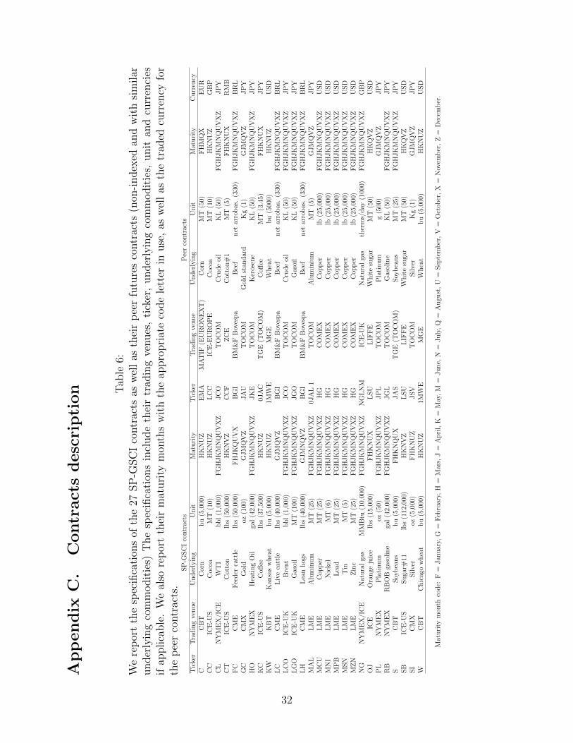
App

endix

C.

Contr

act

sdesc

ripti

on T

able

6:W

ere

por

tth

esp

ecifi

cati

ons

ofth

e27

SP

-GSC

Ico

ntr

acts

asw

ell

asth

eir

pee

rfu

ture

sco

ntr

acts

(non

-index

edan

dw

ith

sim

ilar

under

lyin

gco

mm

odit

ies)

The

spec

ifica

tion

sin

clude

thei

rtr

adin

gve

nues

,ti

cker

,under

lyin

gco

mm

odit

ies,

unit

and

curr

enci

esif

applica

ble

.W

eal

sore

por

tth

eir

mat

uri

tym

onth

sw

ith

the

appro

pri

ate

code

lett

erin

use

,as

wel

las

the

trad

edcu

rren

cyfo

rth

ep

eer

contr

acts

.S

P-G

SC

Ico

ntr

acts

Pee

rco

ntr

acts

Tic

ker

Tra

din

gve

nu

eU

nder

lyin

gU

nit

Mat

uri

tyT

icke

rT

rad

ing

venue

Un

der

lyin

gU

nit

Mat

uri

tyC

urr

ency

CC

BT

Cor

nb

u(5

,000

)H

KN

UZ

EM

AM

AT

IF(E

UR

ON

EX

T)

Cor

nM

T(5

0)F

HM

QX

EU

RC

CIC

E-U

SC

oco

aM

T(1

0)H

KN

UZ

LC

CIC

E-E

UR

OP

EC

oco

aM

T(1

0)H

KN

UZ

GB

PC

LN

YM

EX

/IC

EW

TI

bb

l(1

,000

)F

GH

JK

MN

QU

VX

ZJC

OT

OC

OM

Cru

de

oil

KL

(50)

FG

HJK

MN

QU

VX

ZJP

YC

TIC

E-U

SC

otto

nlb

s(5

0,00

0)H

KN

VZ

CC

FZ

CE

Cot

ton

#1

MT

(5)

FH

KN

UX

RM

BF

CC

ME

Fee

der

catt

lelb

s(5

0,00

0)F

HJK

QU

VX

BG

IB

M&

FB

oves

pa

Bee

fn

etar

robas

.(3

30)

FG

HJK

MN

QU

VX

ZB

RL

GC

CM

XG

old

oz(1

00)

GJM

QV

ZJA

UT

OC

OM

Gol

dst

and

ard

Kg

(1)

GJM

QV

ZJP

YH

ON

YM

EX

Hea

tin

gO

ilga

l(4

2,00

0)F

GH

JK

MN

QU

VX

ZJK

ET

OC

OM

Ker

osen

eK

L(5

0)F

GH

JK

MN

QU

VX

ZJP

YK

CIC

E-U

SC

offee

lbs

(37,

500)

HK

NU

Z0J

AC

TG

E(T

OC

OM

)C

offee

MT

(3.4

5)F

HK

NU

XJP

YK

WK

BT

Kan

sas

wh

eat

bu

(5,0

00)

HK

NU

Z1M

WE

MG

EW

hea

tb

u(5

000)

HK

NU

ZU

SD

LC

CM

EL

ive

catt

lelb

s(4

0,00

0)G

JM

QV

ZB

GI

BM

&F

Bov

esp

aB

eef

net

arro

bas

.(3

30)

FG

HJK

MN

QU

VX

ZB

RL

LC

OIC

E-U

KB

rent

bb

l(1

,000

)F

GH

JK

MN

QU

VX

ZJC

OT

OC

OM

Cru

de

oil

KL

(50)

FG

HJK

MN

QU

VX

ZJP

YL

GO

ICE

-UK

Gas

oil

MT

(100

)F

GH

JK

MN

QU

VX

ZJG

OT

OC

OM

Gas

oil

KL

(50)

FG

HJK

MN

QU

VX

ZJP

YL

HC

ME

Lea

nh

ogs

lbs

(40,

000)

GJM

NQ

VZ

BG

IB

M&

FB

oves

pa

Bee

fn

etar

rob

as.

(330

)F

GH

JK

MN

QU

VX

ZB

RL

MA

LL

ME

Alu

min

um

MT

(25)

FG

HJK

MN

QU

VX

Z0J

AL

1T

OC

OM

Alu

min

ium

MT

(5)

GJM

QV

ZJP

YM

CU

LM

EC

opp

erM

T(2

5)F

GH

JK

MN

QU

VX

ZH

GC

OM

EX

Cop

per

lb(2

5,00

0)F

GH

JK

MN

QU

VX

ZU

SD

MN

IL

ME

Nic

kel

MT

(6)

FG

HJK

MN

QU

VX

ZH

GC

OM

EX

Cop

per

lb(2

5,00

0)F

GH

JK

MN

QU

VX

ZU

SD

MP

BL

ME

Lea

dM

T(2

5)F

GH

JK

MN

QU

VX

ZH

GC

OM

EX

Cop

per

lb(2

5,00

0)F

GH

JK

MN

QU

VX

ZU

SD

MS

NL

ME

Tin

MT

(5)

FG

HJK

MN

QU

VX

ZH

GC

OM

EX

Cop

per

lb(2

5,00

0)F

GH

JK

MN

QU

VX

ZU

SD

MZ

NL

ME

Zin

cM

T(2

5)F

GH

JK

MN

QU

VX

ZH

GC

OM

EX

Cop

per

lb(2

5,00

0)F

GH

JK

MN

QU

VX

ZU

SD

NG

NY

ME

X/I

CE

Nat

ura

lga

sM

MB

tu(1

0,00

0)F

GH

JK

MN

QU

VX

ZN

GL

NM

ICE

-UK

Nat

ura

lga

sth

erm

s/d

ay(1

000)

FG

HJK

MN

QU

VX

ZG

BP

OJ

ICE

Ora

nge

juic

elb

s(1

5,00

0)F

HK

NU

XL

SU

LIF

FE

Wh

ite

suga

rM

T(5

0)H

KQ

VZ

US

DP

LN

YM

EX

Pla

tinu

moz

(50)

FG

HJK

MN

QU

VX

ZJP

LT

OC

OM

Pla

tinu

mg

(500

)G

JM

QV

ZJP

YR

BN

YM

EX

RB

OB

gaso

lin

ega

l(4

2,00

0)F

GH

JK

MN

QU

VX

ZJG

LT

OC

OM

Gas

olin

eK

L(5

0)F

GH

JK

MN

QU

VX

ZJP

YS

CB

TS

oyb

ean

sb

u(5

,000

)F

HK

NQ

UX

JA

ST

GE

(TO

CO

M)

Soy

bea

ns

MT

(25)

FG

HJK

MN

QU

VX

ZJP

YS

BIC

E-U

SS

uga

r#11

lbs

(112

,000

)H

KN

VZ

LS

UL

IFF

EW

hit

esu

gar

MT

(50)

HK

QV

ZU

SD

SI

CM

XS

ilve

roz

(5,0

00)

FH

KN

UZ

JS

VT

OC

OM

Sil

ver

Kg

(1)

GJM

QV

ZJP

YW

CB

TC

hic

ago

wh

eat

bu

(5,0

00)

HK

NU

Z1M

WE

MG

EW

hea

tb

u(5

,000

)H

KN

UZ

US

D

Mat

uri

tym

onth

cod

e:F

=Jan

uar

y,G

=F

ebru

ary,

H=

Mar

s,J

=A

pri

l,K

=M

ay,

M=

Ju

ne,

N=

Ju

ly,

Q=

Au

gust

,U

=S

epte

mb

er,

V=

Oct

ober

,X

=N

ovem

ber

,Z

=D

ecem

ber

.

32

Appendix D. Index investment’s paths to trading venues

Fig. 3:In this functional chart, we describe the various vehicles that commodity index investmentmay use, and how these vehicles hedge on the commodity futures markets, through a portfolioof futures or directly with a futures contract written on the performance of this portfolio.We add the CFTC classification of the categories involved.

Commodity Index Traders (CIT)         

IndividualsInstitutions

mutual funds, hedgefunds, pension funds OTC swap dealers

Exchange tradedproducts (ETF, ETN,

return swaps)

Commodity futuresCommodity indexfutures (SP-GSCI,

BCOM)

CFTC classification level

Centralized market level

Investment vehicle level

Investors

Managedmoney

AssetManager /

InstitutionalSwapdealer

Otherreportables

Dealer /Intermediary

Otherreportables

33

Appendix E. Index investment and arbitrage capital

breaks

Fig. 4:We plot the sums of the monthly total OI and index investment of the 27 SP-GSCI contractsin USD, and their ratios. We add three vertical lines set at the index investment break(August 2003), arbitrage capital break (August 2005) and non significant reversal, that is,the date for which the F-statistic of the Bai et al. (1998) test is maximum in the secondsub-period (August 2011).

inde

x in

vest

men

t sho

ck

arbi

trag

e ca

pita

l sho

ck

inde

x in

vest

men

t rev

ersa

l

0

250

500

750

0

25

50

75

1995 2000 2005 2010 2015date

open

inte

rest

in b

ln. U

SD

ratio (%)

variable

index investment

index investment ratio (right axis)

total open interest

34

App

endix

F.

Vari

able

definit

ion

Tab

le7:

We

defi

ne

all

vari

able

suse

dth

rough

out

the

arti

cle,

wit

hth

eir

sym

bol

s,pla

indefi

nit

ion,

how

we

com

pute

them

(if

applica

ble

),th

eir

unit

s,fr

equen

cy,

per

iod

ofav

aila

bilit

yan

dad

dit

ional

des

crip

tion

sif

nee

ded

.

Sym

bol

Tit

leC

omputa

tion

Unit

Fre

quen

cyP

erio

dD

escr

ipti

on

Fm c,t

Futu

res

pri

ce–

USD

D19

92–

2017

m:

mat

uri

ty,c:

com

modit

y,t:

tim

efm c,t

Log

futu

res

pri

ce–

–D

1992

–20

17–

Rm c,t

Ari

thm

etic

retu

rnRm c,t

=F

m c,t

Fm c,t−1−

1%

D19

92–

2017

We

use

“ret

urn

”fo

rsi

mplici

tybut

itis

am

isnom

er,

“per

cent

pri

cech

ange

”is

mor

eap

pro

pri

ate.

rm c,t

Log

retu

rnrm c,t

=fm c,t−fm c,t−

1%

D19

92–

2017

–SRm c,t

Ari

thm

etic

spre

adin

gre

turn

SRm c,t

=Rm+1

c,t−Rm c,t

%D

1992

–20

17–

srm c,t

Log

spre

adin

gre

turn

srm c,t

=rm

+1

c,t−rm c,t

%D

1992

–20

17–

CASRm c,e

Cum

ula

ted

abnor

mal

spre

adin

gre

turn

sCASRm c,e

=t+τ ∑ t=1

( SRm c,t−Benchmark

c,t)

%M

1992

–20

17e:

even

tm

onth

,τ:

num

ber

ofev

ent

day

s

Bm c,t

Bas

isBm c,t

=( Fm+

1c,t

Fm c,t−

1) ×1

#intervaldays

%D

1992

–20

17W

euse

“Bas

is”

for

sim

plici

tybut

itis

am

isnom

eras

we

use

the

nea

rby

contr

act

topro

xy

for

the

spot

pri

ce.

“Mat

uri

tyra

tio”

ism

ore

appro

pri

ate.

bm c,t

Log

bas

isbm c,t

=( fm+

1c,t−fm c,t) ×

1#intervaldays

%D

1992

–20

17–

Vm c,t

Vol

um

e–

#co

ntr

acts

D19

92–

2017

–CQc

Del

iver

able

quan

tity

––

–19

92–

2017

–CVALm c,t

Con

trac

tva

lue

CVALm c,t

=CQc×Fm c,t

USD

D19

92–

2017

–

XVALm c,t

Con

trac

tva

lue

XVALm c,t

=CQc×Xc,t

USD

D–

For

any

valu

eXc,t

den

omin

ated

in#

ofco

ntr

acts

,th

ere

isaXVALm c,t

den

omin

ated

inU

SD

.TOm c,t

Turn

over

TOm c,t

=CVALm c,t×Vm c,t

USD

D19

92–

2017

–OIm c,t

Op

enin

tere

st–

#co

ntr

acts

D19

92–

2017

Tot

al#

ofco

ntr

acts

open

edin

the

exch

ange

for

each

mat

uri

ty.

TOI c,t

Tot

alop

enin

tere

st–

#co

ntr

acts

D19

92–

2017

Tot

al#

ofco

ntr

acts

open

edin

the

exch

ange

for

all

mat

uri

ties

.

COM

P c,t

Com

mer

cial

pos

itio

n–

#co

ntr

acts

W19

92–

2017

Tot

al#

ofco

ntr

acts

hel

dby

the

“com

mer

cial

”ca

tego

ry,

for

all

mat

uri

ties

.P

stan

ds

for

the

pos

itio

nei

ther

long

(L),

shor

t(S

)or

spre

adin

g(SPREAD

).SPECP c,t

Sp

ecula

tive

pos

itio

n–

#co

ntr

acts

W19

92–

2017

Tot

al#

ofco

ntr

acts

hel

dby

the

spec

ula

tive

cate

gory

for

all

mat

uri

ties

.

ARBc,t

Arb

itra

geca

pit

alra

tio

ARBc,t

=SPEC

SPREAD

c,t

TOI c

,t%∈

[0,1

]W

1992

–20

17T

otal

net

spre

adin

gp

osit

ion

(alw

ays

pos

itiv

e)sc

aled

by

tota

lop

enin

tere

st.

TGSCI t

Tot

alSP

-GSC

Ity

pe

inve

stm

ent

see

app

endix

AU

SD

M19

95–

2017

–GSCIWc,t

Wei

ghts

ofSP

-GSC

I–

%∈

[0,1

]M

1992

–20

17–

GSCI c,t

Am

ount

trac

kin

gSP

-GSC

Ity

pe

funds

GSCI c,t

=GSCIWc,t×TGSCI t

USD

D19

92–

2017

–

INDc,t(1

)In

dex

inve

stm

ent

rati

oINDc,t

=GSCI c

,t

TOI c

,t%∈

[0,1

]W

1992

–20

17–

INDc,t(2

)In

dex

inve

stm

ent

rati

o(a

lter

nat

ive)

INDc,t

=COM

P c,t

TOI c

,t%∈

[0,1

]W

1992

–20

17A

lter

nat

ive

usi

ng

tota

lco

mm

erci

allo

ng

pos

itio

nfr

omth

ele

gacy

rep

ort,

asth

isre

por

tin

cludes

swap

dea

lers

inth

isca

tego

ry.

HPc,t

Hed

ging

pre

ssure

HPc,t

=COM

S c,t−COM

L c,t

COM

S c,t+COM

L c,t

%∈

[−1,

1]W

1992

–20

17–

35

App

endix

G.

CA

Rs

and

CA

SR

sw

ith

alt

ern

ati

ve

bench

mark

s

Tab

le8:

Inth

ista

ble

we

exte

nd

Tab

le3

and

use

five

diff

eren

tb

ench

mar

ks.

The

ben

chm

ark

(1)

ispar

amet

ric.

We

use

indiv

idual

furt

her

def

erre

dco

ntr

acts

asco

vari

ates

(see

app

endix

B)

and

we

esti

mat

eth

em

odel

wit

ha

SU

Rsy

stem

.T

he

ben

chm

arks

(2)

and

(3)

use

the

fact

ors

ofth

eev

ent-

study

ofH

ender

son

etal

.(2

015)

and

thos

eof

the

asse

t-pri

cing

study

ofB

aksh

iet

al.

(201

9).

We

esti

mat

eth

emw

ith

OL

S.

The

ben

chm

ark

(4)

isnon

-par

amet

ric

and

we

use

the

retu

rns

onp

eer

contr

acts

.F

inal

lyth

eb

ench

mar

k(5

)is

aze

ro-b

ench

mar

kto

inve

stig

ate

for

any

model

mis

spec

ifica

tion

.W

ere

por

tth

esa

me

stat

isti

csas

inT

able

3,fo

rth

epre

-,p

ost-

and

roll

win

dow

s.W

eco

mpute

the

CA

SR

sfr

omth

ere

turn

son

the

spre

adin

gp

osit

ion

bet

wee

nth

efirs

tdef

erre

dan

dnea

rby

contr

acts

.In

Pan

elA

,w

ere

stri

ctth

ero

lls

tob

ein

the

Feb

ruar

y–

Dec

emb

erra

nge

,(a

sin

Tab

le3)

while

inP

anel

Bw

ere

por

tth

ere

sult

sfo

rth

ero

llof

Jan

uar

yal

one.

The

per

iod

isfr

omJan

uar

y19

92to

Sep

tem

ber

2017

.R

oll

Pre

-rol

lP

ost-

roll

Pan

elA

(1)

(2)

(3)

(4)

(5)

(1)

(2)

(3)

(4)

(5)

(1)

(2)

(3)

(4)

(5)

CA

SR

%0.

050.

040.

020.

030.

010.

110.

070.

080.

040.

07-0

.06

-0.0

2-0

.03

-0.0

5-0

.09

t-st

atis

tic

2.19

1.99

1.21

0.84

0.30

4.17

2.71

3.10

1.30

3.27

-2.1

3-0

.64

-1.1

4-1

.46

-3.2

5B

MP

0.11

0.10

0.06

0.03

0.01

0.23

0.14

0.16

0.05

0.09

-0.0

9-0

.03

-0.0

5-0

.04

-0.1

1K

P0.

050.

080.

030.

020.

000.

110.

120.

080.

030.

05-0

.04

-0.0

2-0

.02

-0.0

2-0

.05

R2

%2.

604.

684.

682.

634.

704.

702.

634.

724.

70P

anel

B

CA

SR

%0.

060.

000.

080.

020.

060.

100.

000.

070.

040.

08-0

.08

0.00

-0.0

1-0

.02

-0.1

1t-

stat

isti

c1.

200.

001.

680.

301.

361.

190.

000.

840.

491.

00-1

.36

0.00

-0.1

6-0

.23

-1.5

1B

MP

0.10

0.00

0.14

0.02

0.10

0.13

0.00

0.08

0.04

0.10

-0.0

80.

00-0

.01

-0.0

1-0

.09

KP

0.03

0.00

0.06

0.01

0.04

0.04

0.00

0.03

0.02

0.04

-0.0

30.

000.

00-0

.01

-0.0

3R

2%

3.94

8.12

8.05

3.95

8.13

8.06

3.97

8.15

8.07

36