Comments on “Robust Bond Risk Premia” by Michael

Bauer and Jim Hamilton

John H. Cochrane∗

November 6, 2015

1. Questions

The questions to answer are straightforward: What do we learn about bond return or

yield change predictability? In particular, do macro variables or yield information past

3 principal components help to forecast bond returns and/or yield changes? And, the

point of the paper: what do we learn about econometric or empirical pitfalls from this

case, lessons that may be more generally useful?

I’ll focus on the Joslin, Priebsch, Singleton (2014) regressions. These are forecasting

regressions, for example

rxt+1 = a+ b′1PCt + b′2[GROt INFt] + b′3(more yieldst) + εrt+1

where rx is a bond excess return, PC are the three first principal components of bond

yields, GRO is a measure of economic growth, and INF is a measure of inflation.

The question is whether growth and inflation, or information in yields past the first

three principal components, are useful additional forecasters. Joslin, Priebsch, Single-

ton famously concluded that macro variables are important in addition to yields for

describing bond risk premiums. Bauer and Hamilton question that finding. Let’s dig

in.∗Hoover Institution and NBER. Comments presented at the 5th Conference on Fixed Income Markets,

Federal Reserve Bank of San Francisco, November 5 2015. Bauer and Hamilton’s paper is available at http://www.frbsf.org/economic-research/files/wp2015-15.pdf

1

2

The questions are broader. This sort of regression is also used to forecast changes

in yields,

yt+1 − yt = a+ b′1PCt + +b′2[GROt INFt] + b′3(more yieldst) + εyt+1

By standard identities, return forecast and yield change forecast regressions are basi-

cally the same thing. The presence of inflation and growth as macro variables suggests

a tantalizing link to Taylor rules,

yt+1 − yt = a+ φy ×GROt+1 + φπ × INFt+1 + (+ yields?) + εyt+1

2. Facts

So, do macro variables help? I noticed quickly Bauer and Hamilton’s Table 4:

There are two lessons here: First, the Joslin, Priebsch and Singleton macro variable

estimates are greatly reduced out of sample. That’s an empirical, not an econometric

issue.

Second, and Bauer and Hamilton’s focus, the remaining rise in R2 when we add

macro variables is now statistically insignificant.

Bauer and Hamilton kindly provided me with the data, so I was able to investigate

3

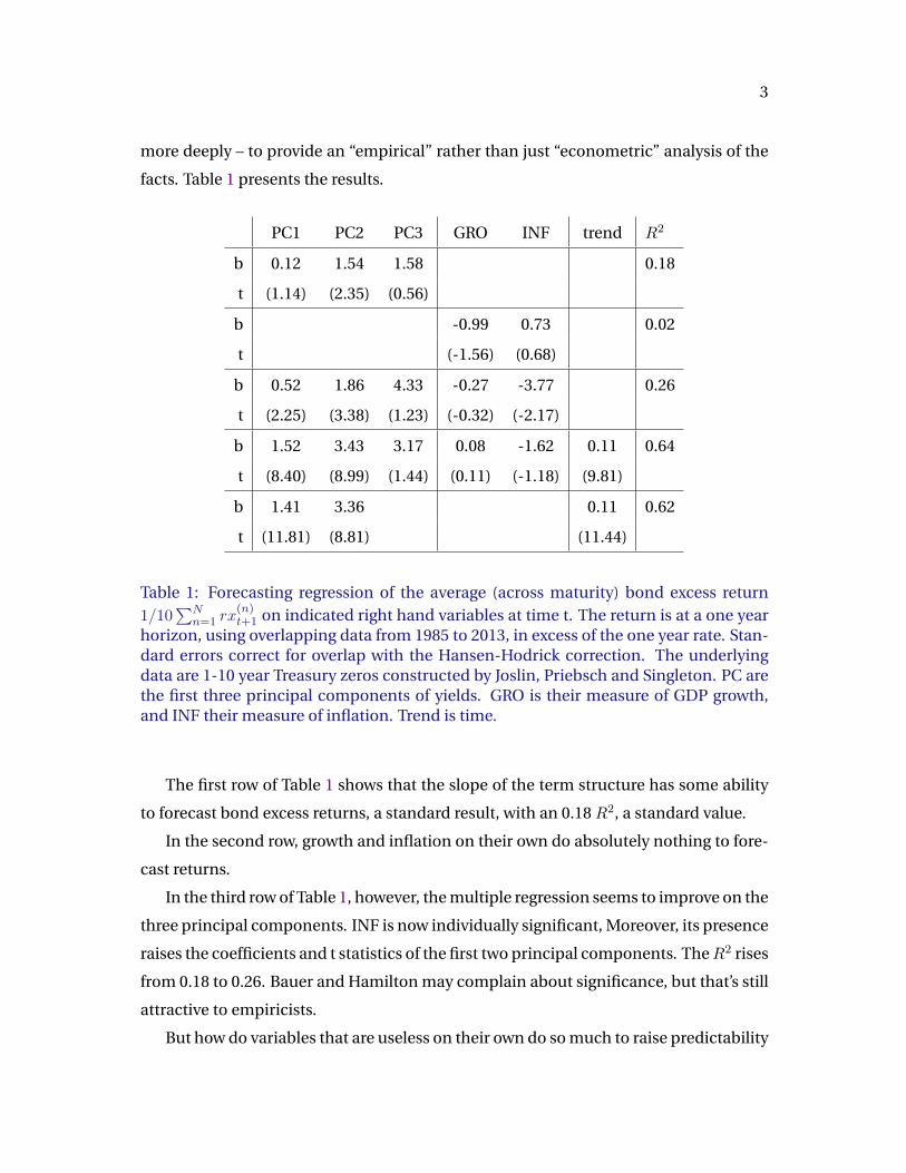
more deeply – to provide an “empirical” rather than just “econometric” analysis of the

facts. Table 1 presents the results.

PC1 PC2 PC3 GRO INF trend R2

b 0.12 1.54 1.58 0.18

t (1.14) (2.35) (0.56)

b -0.99 0.73 0.02

t (-1.56) (0.68)

b 0.52 1.86 4.33 -0.27 -3.77 0.26

t (2.25) (3.38) (1.23) (-0.32) (-2.17)

b 1.52 3.43 3.17 0.08 -1.62 0.11 0.64

t (8.40) (8.99) (1.44) (0.11) (-1.18) (9.81)

b 1.41 3.36 0.11 0.62

t (11.81) (8.81) (11.44)

Table 1: Forecasting regression of the average (across maturity) bond excess return1/10

∑Nn=1 rx

(n)t+1 on indicated right hand variables at time t. The return is at a one year

horizon, using overlapping data from 1985 to 2013, in excess of the one year rate. Stan-dard errors correct for overlap with the Hansen-Hodrick correction. The underlyingdata are 1-10 year Treasury zeros constructed by Joslin, Priebsch and Singleton. PC arethe first three principal components of yields. GRO is their measure of GDP growth,and INF their measure of inflation. Trend is time.

The first row of Table 1 shows that the slope of the term structure has some ability

to forecast bond excess returns, a standard result, with an 0.18 R2, a standard value.

In the second row, growth and inflation on their own do absolutely nothing to fore-

cast returns.

In the third row of Table 1, however, the multiple regression seems to improve on the

three principal components. INF is now individually significant, Moreover, its presence

raises the coefficients and t statistics of the first two principal components. TheR2 rises

from 0.18 to 0.26. Bauer and Hamilton may complain about significance, but that’s still

attractive to empiricists.

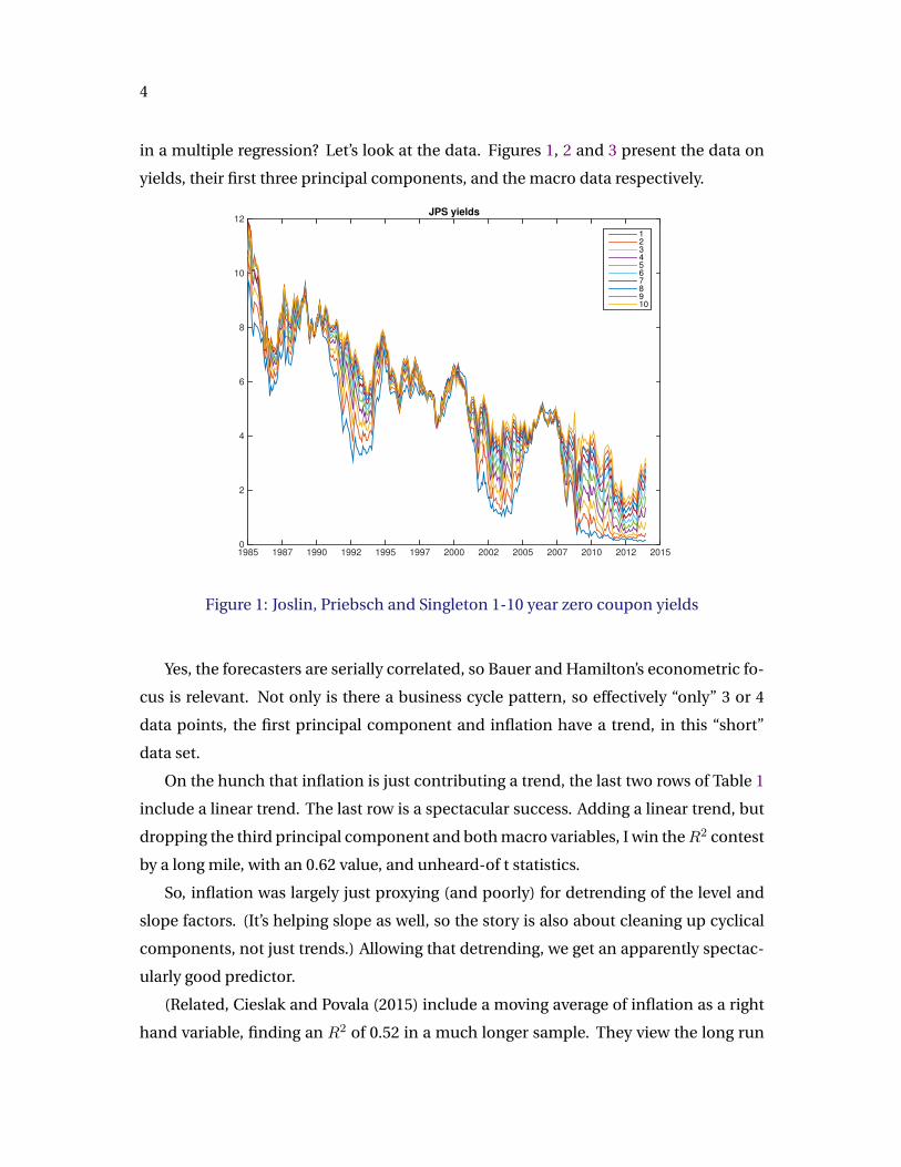
But how do variables that are useless on their own do so much to raise predictability

4

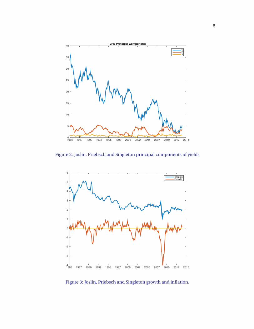
in a multiple regression? Let’s look at the data. Figures 1, 2 and 3 present the data on

yields, their first three principal components, and the macro data respectively.

1985 1987 1990 1992 1995 1997 2000 2002 2005 2007 2010 2012 20150

2

4

6

8

10

12JPS yields

1

2

3

4

5

6

7

8

9

10

Figure 1: Joslin, Priebsch and Singleton 1-10 year zero coupon yields

Yes, the forecasters are serially correlated, so Bauer and Hamilton’s econometric fo-

cus is relevant. Not only is there a business cycle pattern, so effectively “only” 3 or 4

data points, the first principal component and inflation have a trend, in this “short”

data set.

On the hunch that inflation is just contributing a trend, the last two rows of Table 1

include a linear trend. The last row is a spectacular success. Adding a linear trend, but

dropping the third principal component and both macro variables, I win theR2 contest

by a long mile, with an 0.62 value, and unheard-of t statistics.

So, inflation was largely just proxying (and poorly) for detrending of the level and

slope factors. (It’s helping slope as well, so the story is also about cleaning up cyclical

components, not just trends.) Allowing that detrending, we get an apparently spectac-

ularly good predictor.

(Related, Cieslak and Povala (2015) include a moving average of inflation as a right

hand variable, finding an R2 of 0.52 in a much longer sample. They view the long run

5

1985 1987 1990 1992 1995 1997 2000 2002 2005 2007 2010 2012 20150

5

10

15

20

25

30

35

40JPS Principal Components

1

2

3

Figure 2: Joslin, Priebsch and Singleton principal components of yields

1985 1987 1990 1992 1995 1997 2000 2002 2005 2007 2010 2012 2015-4

-3

-2

-1

0

1

2

3

4

5

6

InflationGrowth

Figure 3: Joslin, Priebsch and Singleton growth and inflation.

6

movements in the level factor as arising from inflation, so adding inflation to the re-

gression removes low frequency nominal movements from the level factor, leaving the

real movements that correspond to changing risk premiums. The point is not whether

a trend or long-run inflation is the “right” forecaster. The point is that inflation helps

yields to forecast returns by removing a very slowly moving component of yields.)

Perhaps this result is just due to a few data points? Another good empirical check is

a plot of forecast and actual, to make sure any pattern is regular over the span of data.

Figure 4 presents ex-post returns together with their forecast. On the top left, we see

that the principal components do forecast returns. On the top right, we see that GRO

and INF by themselves do essentially nothing. On the bottom left, we see the improved

forecasts including both principal components and macro data.

But on the bottom right, we see the spectacular performance of the first two princi-

pal components plus the trend. The forecast is not matching a trend in returns – that’s a

cheap way to get highR2. The forecast really is cleaning up a higher frequency variation

of PC1 and PC2. The improvement is consistent over episodes.

(You may worry a bit about standard error corrections for serial correlation due to

overlap. It’s well known that the Hansen-Hodrick or Newey-West nonparametric cor-

rections sometimes behave poorly. For a while I thought that’s what Bauer and Hamil-

ton were about. But that really isn’t the issue. In this case, I ran all the regressions from

January to January. I also did Jan-Jan, Feb-Feb, etc. regressions and present the aver-

age of these results. These nonoverlapping regressions are a bit less efficient, but the

standard errors can be computed using only OLS formulas.

Table 2 shows the first row of Table 1 redone this way, and you can see the results

are unaffected. The same holds for the other rows.)

3. Econometrics

Now, how do we interpret these results? Is the trend forecast a proof that macro vari-

ables really don’t matter, because they can be driven out by a simple trend? Is the result

thus a reductio ad absurdum? Is the result a brilliant demonstration that information

in yields, beyond the first three principal components, can help significantly to forecast

yields – that time-filtered principal components are the hot forecasters?

7

1985 1990 1995 2000 2005 2010 2015-10

-5

0

5

10

15

20

253 PC

rxt+1

a+b'xt

1985 1990 1995 2000 2005 2010 2015-10

-5

0

5

10

15

20

25GRO and INF

1985 1990 1995 2000 2005 2010 2015-10

-5

0

5

10

15

20

253 PC, GRO and INF

1985 1990 1995 2000 2005 2010 2015-10

-5

0

5

10

15

20

25PC1, PC2, Trend

Figure 4: Forecast a+ bxt and actual rt+1 returns

8

Method PC1 PC2 PC3 R2

Jan-Jan b 0.16 1.51 0.72 0.17

t (1.71) (2.16) (0.17)

Av Mo. b 0.12 1.55 1.72 0.20 (av. mo.)

t (1.71) (2.16) (0.17) 0.18 (same b)

Overlap b 0.12 1.54 1.58 0.18

t (1.14) (2.35) (0.56)

Table 2: Comparison of January-January nonoverlapping forecasts, average of allmonth-month nonoverlapping forecasts, and overlapping forecasts with Hansen-Hodrick correction. “av.mo” gives the average R2 in month-to-month regressions,“same b” gives the R2 forcing each month to use the same value of b.

Or, is the result a first-order econometric goof? Surely if forecasting with persistent

but stationary variables causes problems, forecasting in-sample trends with near-unit

roots floating around should raise fire alarms! That’s what Bauer and Hamilton’s paper

is about. So let’s see what the paper has to say.

What are, really, the dangers of forecasting with highly serially correlated right hand

variables?

Consider the system

rt+1 = b1xt + b2yt + εrt+1

xt+1 = ρxxt + εxt+1

yt+1 = ρyxt + εyt+1

(I suppress constants for simplicity.) The null hypothesis is that b2 = 0, and that re-

turns are not forecastable from anything, in particular they are uncorrelated over time,

cov(εrt+1, anythingt) = 0.

Now, it’s very intuitive that slow-moving forecasters cause trouble. If there are only a

few business cycles or zero crossings in yt it seems that there are really few data points,

and we really don’t know that much. But econometrics reminds us of a hard fact:

For fixed x and y, OLS is BLUE, and OLS standard errors are correct. Deeply, OLS

9

does not care about the ordering of right hand variables. OLS and its standard errors

are exactly the same if we reshuffle random variables in any order. Distribution theory

revolves around the correlation properties of the error term, not those of the right hand

variable.

You’re probably still queasy about regressions on trends or highly correlated right

hand variables. In cross-sectional regressions, you are queasy if you discover that a

right hand variable in a county-level regression is all positive on the west of the Missis-

sippi and negative on the east – strong cross-sectional correlation. But if the errors are

uncorrelated, OLS does not care. You should be queasy, but we’ll have to look elsewhere

to understand why.

With stochastic x and y – with a distribution theory that resamples x and y, not just

the errors – this theorem is no longer true. The coefficients are consistent, but not

necessarily unbiased, and the OLS standard errors are asymptotically valid, but not in

finite sample.

And there is a well-known finite sample problem: If the forecaster error εy and the

return error εr are strongly negatively correlated, then the coefficient b2 on y is biased

up. This is the famous Stambaugh bias. The intuition is straightforward: With a near-

unit root, the autocorrelation coefficient ρy is downward biased. This means that yt

and εyt+1 are negatively correlated. In turn, if the errors εy εr are negatively correlated,

then yt and εrt+1 are positively correlated, resulting in upward bias of the return-forecast

coefficient.

That correlation may hold for price variables. When returns are unexpectedly high,

prices are unexpectedly low, so the needed negative correlation is often there. So far

the consensus (well, my consensus, see Cochrane (2008)!) has been that the effect is

not strong enough to overturn the evidence for price-dividend ratio based stock market

predictability. But the bias is there.

But macro variables do not have errors that are strongly negatively correlated with

returns. So Stambaugh bias does not apply. Bauer and Hamilton’s paper is explicitly

not about Stambaugh bias:

... the problem with hypothesis tests of β2 = 0 does not arise from Stam-

baugh bias as traditionally understood. Instead of coefficient bias, the rea-

son for the size distortions of these tests is the fact that the OLS standard

10

errors substantially underestimate the sampling variability of both b1 and

b2.

The paper is about the distribution of a macro variable, whose errors are uncorrelated

with return errors, in the presence of a price variable, whose errors are so correlated.

The setup is corr(εrt+1, εyt+1) = 0, but corr(εrt+1, ε

yt+1) < 0. Then, apparently, b2 remains

unbiased, but its standard errors are too small, and thus R2 can be too big – we see

unexpectedly many large b2 in both directions.

I don’t have intuition for this result, as I presented for the Stambaugh bias. I pre-

sume it’s something about near unit root large non-normal errors in εxt+1, εyt+1 feed in

to εrt+1

But how big is this effect? Is this enough to unwind the 8.0 t statistics and make a

fool of my trend-based forecasts? I did my own little Monte Carlo, more attuned to the

return-forecasting question than the simulations in Bauer and Hamilton’s paper, and

Figure 5 presents the results.

−0.5 0 0.5 10

1

2

3

4

5

6

7

b

b1, cov(e

x,e

y,e

r) = 0

b1 cov(e

x e

r) = −0.9

b2 cov( e

x e

r)=−0.9

Figure 5: Monte Carlo distribution of return-forecasting coefficient

11

I simulate the following system, for 30 periods:

rt+1 = b1xt + b2yt + εrt+1

xt+1 = 0.95xt + εxt+1

yt+1 = 0.95yt + εyt+1

I set b1 = b2 = 0 to simulate, and then estimate the regressions in simulated data, with

constants.

First, I set the correlation of all the errors to zero. The blue line of Figure 5 gives

the distribution of b2 in this case. (It’s the same as the distribution of b1.) You see it’s

unbiased and nicely normal.

Next, I raise the (negative) correlation between return and price-variable shocks,

corr(εr, εx) to = −0.9. The red line graphs the resulting distribution of the x coefficient

b1. Here you see the quite serious Stambaugh bias. The mode of the distribution is

about b1 = 0.1, around one standard error above zero. And the distribution is spread

out as well. This variable would have spuriously large R2 as well as spuriously large

regression coefficients.

But our issue is the distribution of b2, the coefficient on an additional variable, also

serially correlated, but whose errors are not correlated with those of returns or of prices.

This distribution is shown in the magenta line of Figure 5. Yes, the distribution is a bit

wider. But the effect is very small. And -0.9 error correlation, with 0.95 serial correlation

and 30 years of data seem like a pretty trying environment.

Figure 6 shows the worst-case scenario: both forecasters x and y are random walks,

and the correlation between return and x innovations is -1. I still am not finding a huge

distortion, or anything near the effects of Stambaugh bias.

So, I remain to be persuaded just what this effect is, and that it is quantitatively

significant for addressing the issues raised in bond-return forecasting regressions.

3.1. Fear of serially correlated forecasters

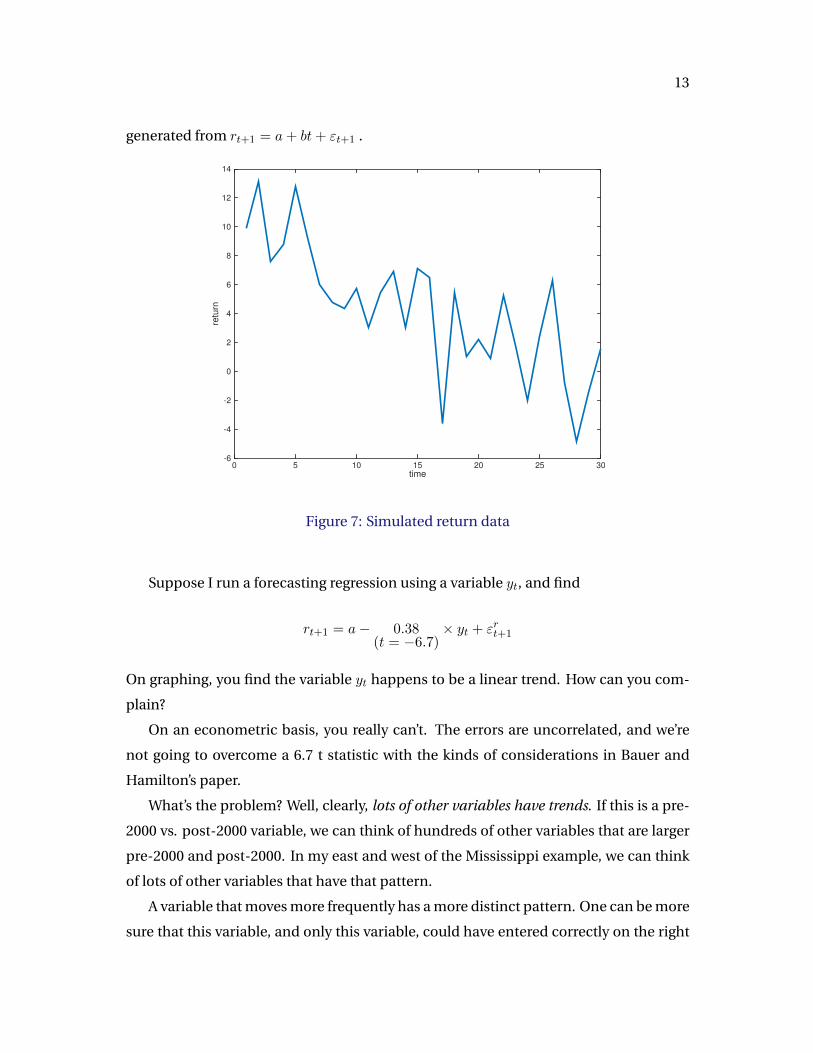
Why are we then so rightly suspicious of forecasters that are highly serially correlated,

even if the errors are not serially correlated? (Both in the time series and in the cross

section.) As a hypothetical, suppose you see return data as shown in Figure 7, which I

12

−0.5 0 0.5 10

1

2

3

4

5

6

7

b

b1, cov(e

x,e

y,e

r) = 0

b1 cov(e

x e

r) = −0.9

b2 cov( e

x e

r)=−0.9

Figure 6: Monte Carlo distribution of return-forecasting coefficient, with random walkforecasters and perfect residual correlation

13

generated from rt+1 = a+ bt+ εt+1 .

time

0 5 10 15 20 25 30

retu

rn

-6

-4

-2

0

2

4

6

8

10

12

14

Figure 7: Simulated return data

Suppose I run a forecasting regression using a variable yt, and find

rt+1 = a− 0.38(t = −6.7)

× yt + εrt+1

On graphing, you find the variable yt happens to be a linear trend. How can you com-

plain?

On an econometric basis, you really can’t. The errors are uncorrelated, and we’re

not going to overcome a 6.7 t statistic with the kinds of considerations in Bauer and

Hamilton’s paper.

What’s the problem? Well, clearly, lots of other variables have trends. If this is a pre-

2000 vs. post-2000 variable, we can think of hundreds of other variables that are larger

pre-2000 and post-2000. In my east and west of the Mississippi example, we can think

of lots of other variables that have that pattern.

A variable that moves more frequently has a more distinct pattern. One can be more

sure that this variable, and only this variable, could have entered correctly on the right

14

hand side.

However, that’s still not a satisfactory answer in this case. For structural work, yes,

we may not have the “real” causal variable. But here, we don’t care about real causes.

We only care about forecasting. Already, we include bond factors, knowing those factors

proxy for, and reveal, the real variables. So if we have proxy variables already, is serial

correlation really a problem?

Really, the problem is, that we could have found so many other similar variables.

If the data had a significant V shaped pattern, we could have found that. If they were

higher on even vs. odd years, we would have found that. That’s the sense in which it is

“easy” to find these results. This is really a specification problem, not an econometric

problem.

Traditionally, the main guard against this kind of fishing has been an economic in-

terpretation of the forecasting variable. But that discipline is dying out, with the result

that we have hundreds of claimed forecasting variables.

4. Bigger dangers

I think this quest for statistical significance in a multiple regression sense also takes

us away from the many empirical and econometric problems remain with forecasting

regressions, that could use some econometric guidance.

Figure 8 presents the forward rates from the Joslin, Priebsch and Singleton data. You

can see a lot of small high frequency up and down jumpiness. This data has either high

frequency measurement error, or small high frequency idiosyncratic price movements

that provide lovely near-arbitrage opportunities for traders.

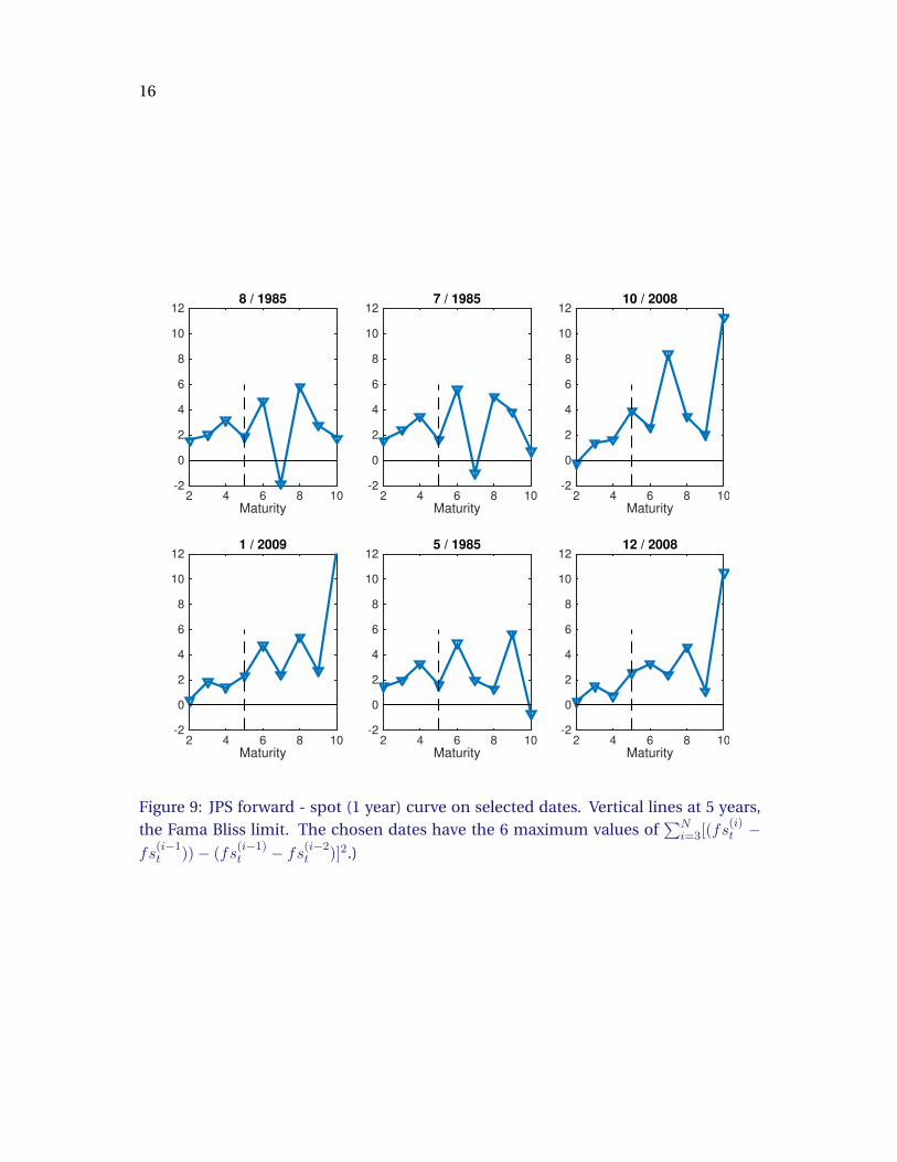
Slicing the data horizontally, things get worse. Figure 9 shows the forward curve on

selected dates. These forward curves jump all over the place, with the zig-zag pattern

characteristic of idiosyncratic price measurement error – or arbitrage opportunity. The

vertical line of figure 9 shows the limit of the Fama-Bliss (1986) procedure, and you can

see why they chose to stop at 5 years. (My first stab at this discussion was to extend

regressions of returns on forward rates, as in Cochrane-Piazzesi (2008). Figure 9 put a

quick stop to that project.)

These small idiosyncratic price changes melt away quickly. Thus, if measurement

15

1985 1987 1990 1992 1995 1997 2000 2002 2005 2007 2010 2012 2015-0.04

-0.02

0

0.02

0.04

0.06

0.08

0.1

0.12

0.14JPS Forward-spot spreads

2

3

4

5

6

7

8

9

10

Figure 8: Forward rates less one year yield in Joslin Priebsch and Singleton data

error, these small pricing errors induce spurious high-Sharpe-ratio short-run predictabil-

ity, as emphasized by Figure 10. If arbitrage opportunities, they introduce features that

arbitrage-free models cannot capture.

Empiricists employ a suite of ad-hoc procedures to deal with this measurement er-

ror problem: We estimate directly at a one-year horizon rather than estimate at the

theoretically more efficient one-month horizon and raise results to the 12th power. We

use moving averages or lags of yields to forecast, rt+1 = a + b(yt + yt−1) + εt+1, since

moving averages smooth out the measurement error and lagged yields do not share a

mismeasured endpoint with their return. We use splines or principal components to

smooth the data, but risk throwing the baby out with the bathwater.

All of these are ad-hoc procedures though. Real help from real econometricians

would be valuable! (Pancost 2015 estimates a yield curve model using the underlying

coupon bond prices, allowing for measurement error, which is a pure, but complex,

solution to these problems.)

16

Maturity2 4 6 8 10

-2

0

2

4

6

8

10

128 / 1985

Maturity2 4 6 8 10

-2

0

2

4

6

8

10

127 / 1985

Maturity2 4 6 8 10

-2

0

2

4

6

8

10

1210 / 2008

Maturity2 4 6 8 10

-2

0

2

4

6

8

10

121 / 2009

Maturity2 4 6 8 10

-2

0

2

4

6

8

10

125 / 1985

Maturity2 4 6 8 10

-2

0

2

4

6

8

10

1212 / 2008

Figure 9: JPS forward - spot (1 year) curve on selected dates. Vertical lines at 5 years,the Fama Bliss limit. The chosen dates have the 6 maximum values of

∑Ni=3[(fs

(i)t −

fs(i−1t ))− (fs

(i−1)t − fs(i−2t )]2.)

17

positive price error at t

Spuriously forecasts return at t+1

Figure 10: Small “measurement” errors lead to spurious (arbitrage or near-arbitrage)return forecastability.

5. Bigger questions

I think we are also focusing on the wrong questions. Here, the question is parsimony,

measuring whether additional variables in a single asset’s return-forecasting equation

are statistically significant. In

rxt+1 = a+ bxt + cyt + εrt+1

does yt enter with statistical significance?

For forecasting, not structural purposes, though, this is a bit of an old-fashioned

question. Since Sims (1980) introduced VARs, the fashion in forecasting has been to

accept slightly overparameterized right hand variables, many of them with admitted

t statistics well below the magic 2.0 values. Their coefficients will be small, and they

typically don’t change forecasts that much. Sure, the in-sample R2 will be overstated a

bit. But just what harm lies in that fact?

Some of the habit, I think, goes back to efficient-markets debates from the 1970s

and 1980s, when testing the null that returns are not at all predictable was interesting.

But that debate is over. Returns are predictable. The issue now is characterizing that

predictability.

18

5.1. Factor structure of expected returns

The first bigger question is the factor structure of expected returns. Figure 11 illustrates

the issue. Here I plot the fitted value of the admittedly overparameterized JPS regres-

sion, for each of the 10 bonds, the right hand side of

rx(n)t+1 = a(n) + b(n)[PC1t PC2t PC3t] + c(n)[GROt INFt] + ε

(n)t+1. (1)

1985 1987 1990 1992 1995 1997 2000 2002 2005 2007 2010 2012 2015

-5

0

5

10

15

20Expected returns from PC1 PC2 PC3 GRO INF

Figure 11: Fitted values of excess return-forecasting regressions for 1-10 year Treasuryzeros. The regressions are rx(n)t+1 = a(n)+b(n)[PC1t PC2t PC3t]+c

(n)[GROt INFt]+ε(n)t+1.

You can see the pattern. Despite 5 right hand variables, so potentially 5 different

sources of movement, and despite an arguably overparameterized regression, there is

a clear one-factor structure of expected returns. The expected returns on all maturities

move in lockstep, with longer maturities moving more than shorter maturities. The

regressions (1) (note plural) really want to be

rx(n)t+1 = γ(n) {a+ b[PC1t PC2t PC3t] + c[GROt INFt]}+ ε

(n)t+1. (2)

19

This is a restriction across maturities n, across regressions being run at the same time,

not a restriction on the identities of right hand side variables.

This one-factor structure of expected returns, not the presence of higher-order fac-

tors on the right hand side, or their tent-shaped coefficients, was the major message of

Cochrane and Piazzesi (2005), (2008).

Most econometrics thinks about the regressions (1) one at a time, and asks about

adding right hand variables. We need to ask a completely different question. We need

to ask about the commonality of fitted values across 10 different left-hand variables

that are being fit at the same time.

In words, rather than ask “what is the exact set of forecasting variables that we

should use to forecast a given return,” we ask here “what is the linear combination

of forecasting variables that captures common movement in expected returns across

assets.”

Unconditional asset pricing did this in the 1970s and 1980s. Econometrics was

based on one equation at a time, y = a + xb + ε. Finance thought about many assets

at once. When finance researchers ran Rit = αi + βiRemt + εit, it turned out econometri-

cians had never thought to characterize the joint distribiution of regression intercepts

αi across regressions. So finance researchers stepped in, first Fama and MacBeth, then

Gibbons Ross and Shanken, and then Hansen GMM.

Here we face conditional versions of the same issue. Here we are, thinking about

forecasting one return at a time, not thinking about how expected returns of different

assets move together. It’s time to move on!

We’re just beginning to understand this question. It looks so far like there is a domi-

nant single factor for bond returns – risk premiums rise and fall together. Is that conclu-

sion correct? Are there additional factors that move some expected returns one way and

other expected returns another way? In fact, eigenvalue decomposing the right hand

side of (1), the first two eigenvalues account for 97.14% and 2.59% of the variance re-

spectively (this is the squared eigenvalue divided by the sum of squared eigenvalues of

the covariance matrix of fitted values.) Cochrane and Piazzesi (2008) found more than

99% from the first factor, but did not have macro variables. Is there a second macro

factor in expected returns? Or is that finding insignificant? This is a question on which

I surely would like some econometric help!

20

Once we find the factor structure in bonds, what is the factor structure of expected

returns across asset classes? Do stock expected returns and bond expected returns

move one for one? Here, as in all factor analysis, parsimony really is important. How

many factors do we really need?

5.2. Means and covariances

The second big question is, what are the factors, covariance with which drives variation

in expected returns? What are the F in

Et(r(n)t+1) = cov(r

(n)t+1, Ft+1)λt?

This is The Question of finance, really. We should answer it. Cochrane and Piazzesi

(2008) concluded that there is a single factor model of expected returns, and that all

expected returns results from covariance with shocks to the level factor. Is this right?

How do macro variables fit in to this picture? What are the econometric issues in such

an investigation? How do we do conditional Gibbons-Ross-Shanken or, better, GMM?

Estimates are easy and suggestive. I eigenvalue decompose the right hand side of

(1), i.e.

QΛQ′ = eig[

cov(a(n) + b(n)[PC1tPC2tPC3t] + c(n)[GROtINFt]

)]. (3)

where the cov operator produces a 10× 10 covariance matrix of expected returns.

Denote by q the 10× 1 column of Q corresponding to the largest eigenvalue. I form

the expected return factor as

Ert ≡ q′(a(n) + b(n)[PC1t PC2t PC3t] + c(n)[GROt INFt]

)Then, I form the one-factor model of expected returns by running for each n,

rx(n)t+1 = γ(n)Ert + ε

(n)t+1. (4)

(One can also infer the γ(n) coefficients, but it’s more intuitive to run the regression

again.)

21

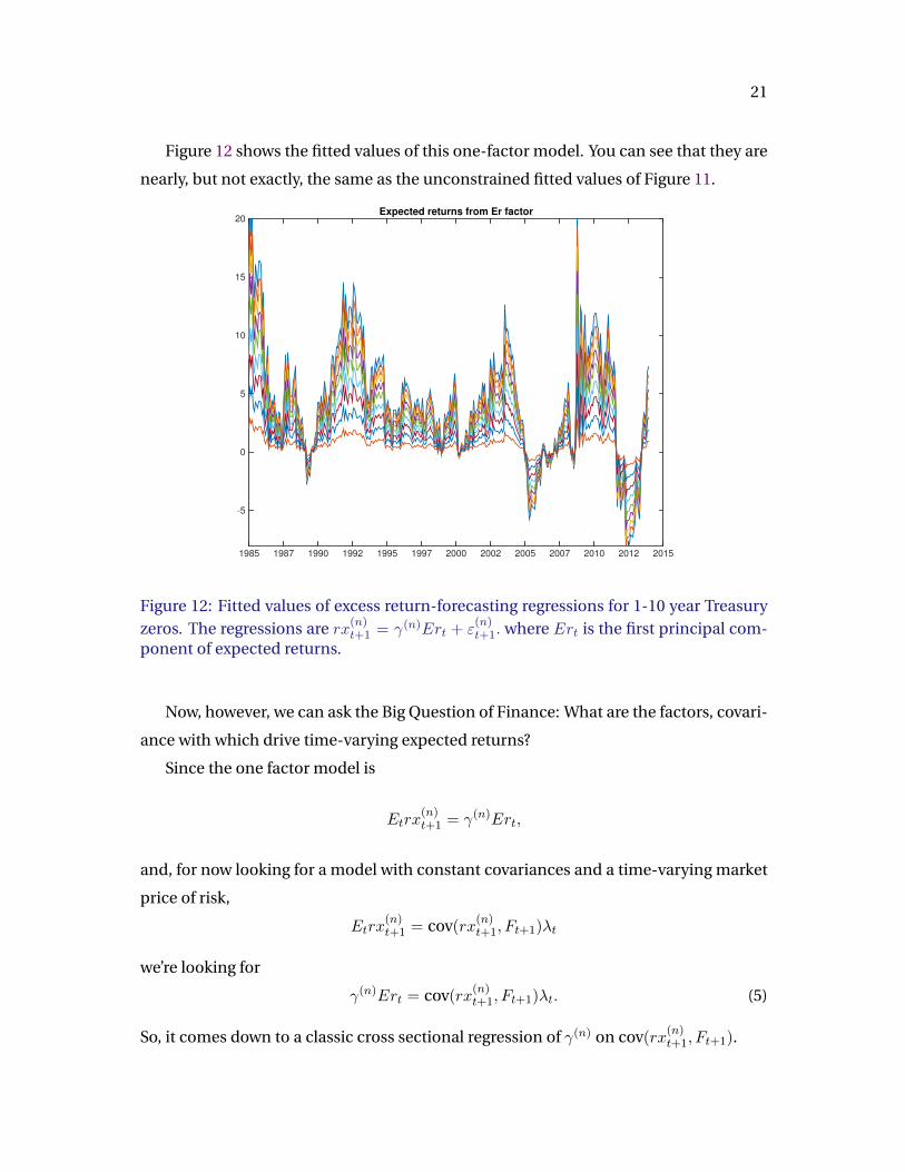
Figure 12 shows the fitted values of this one-factor model. You can see that they are

nearly, but not exactly, the same as the unconstrained fitted values of Figure 11.

1985 1987 1990 1992 1995 1997 2000 2002 2005 2007 2010 2012 2015

-5

0

5

10

15

20Expected returns from Er factor

Figure 12: Fitted values of excess return-forecasting regressions for 1-10 year Treasuryzeros. The regressions are rx(n)t+1 = γ(n)Ert + ε

(n)t+1. where Ert is the first principal com-

ponent of expected returns.

Now, however, we can ask the Big Question of Finance: What are the factors, covari-

ance with which drive time-varying expected returns?

Since the one factor model is

Etrx(n)t+1 = γ(n)Ert,

and, for now looking for a model with constant covariances and a time-varying market

price of risk,

Etrx(n)t+1 = cov(rx

(n)t+1, Ft+1)λt

we’re looking for

γ(n)Ert = cov(rx(n)t+1, Ft+1)λt. (5)

So, it comes down to a classic cross sectional regression of γ(n) on cov(rx(n)t+1, Ft+1).

22

I run a first order VAR of the 5 Joslin, Priebsch and Singleton factors to generate

shocks. Then, I calculate the covariance of each of the 1-10 year maturity bond excess

returns with those factor shocks. This produces an estimate of the covariance of returns

with the 5 factors cov(rx(n)t+1, Ft+1).

Figure 13 plots these covariances on the x axis against the loading γ(n) of each return

on the first expected return factor on the y axis. Through the eyes of (5) these are the

“expected returns” which should line up with the “betas.”

Covariance of excess return with factors-5 0 5 10 15 20 25

Exp

ecte

d r

etu

rn f

acto

r lo

ad

ing

γ

0

0.5

1

1.5

2

2.5

PC1PC2PC3GROINF

Figure 13: Covariance of excess bond returns (maturity 1-10 years) with innovations in5 JS factors, vs. loading γ(n) on the return-forecasting factor Ert.

Figure 13 has the same result as Cochrane and Piazzesi (2008): Time-varying ex-

pected bond returns are earned entirely as compensation for level risk.

One can put the same point in a multiple cross sectional regression. Table 3 presents

the coefficients in a multiple regression of γ(n) on the covariances cov(rx(n)t+1, Ft+1) of the

10 bond returns on the 5 factors. The table verifies the impression of the figure: only

covariances with the level factor matter.

I won’t even try to assign standard errors or test statistics for the purpose of this

discussion. Obviously, doing so correctly, including the in-sample factor analysis, is a

23

PC1 PC2 PC3 GRO INF

10.52 0.35 -0.23 1.07 0.92

Table 3: Multiple regression coefficients of factor loadings on the expected return factorγ(n) against covariances of excess returns with shocks to factors. These cross sectionalregressions are over 10 bond maturities.

delicate undertaking. Which is my point. This is an issue on which we need serious

econometric help!

All of this is input to practical analysis, such as decompositions of the yield curve

into expectations and risk premium components. Such decompositions are routinely

presented with no standard errors at all, and with many decimal points, which is how

you know financial economists have a sense of humor. Obviously, there is an important

econometric challenge.

These are simple, but suggestive calculations. I make them here to make the point

– this is easy to do. It’s time to do it. Let’s move on to these important questions, rather

than stop at the the very first step, statistical significance of extra predictors in one-

asset-at-a-time return forecasting regressions.

6. Spanning

Both papers address the “spanning” proposition that bond yields reflect all informa-

tion that macro variables could possibly have for bond expected returns. This is one of

the first tricks you learn in term structure modeling: Write down a model with latent

(unobserved) state variables X, derive prices as functions P (X) of the latent state vari-

ables, and then invert this function so that prices or yields become the state variables.

While a neat trick, this property implies that although variables such as GRO and INF

may be important structural determinants of expected returns or yield changes, they

will always be at least equaled and likely dominated as reduced-form forecasters by

bond yields themselves.

But while this is a neat trick, there is no reason in general that macro variables or

small yield movements past the big principal components should not help to forecast

24

returns or yield changes. So, both papers address simple “fact” questions, with no deep

theory at stake. The spanning property is an artifact of finite number of underlying

state variables, an exact factor structure, and restrictions on market prices of risk.

Intuitively, like short-lasting changes in volatility, temporary variation in risk premi-

umsEt(rt+1) contributes little to the level of prices Pt. The variance of expected returns

is much smaller than the variance of ex-post returns.

More generally, there is no reason that factors which explain most of the variance of

the predictors var(yt) should capture most of their predictive ability, varEt(rt+1|yt).

Here is a simple example, following Cochrane and Piazzesi (2008, p.9 ff). I leave out

the constants which needlessly complicate the formulas.

The model: A vector of state variablesXt follows a vector AR(1) with normal shocks,

Xt+1 = φXt + vt+1;E(vt+1v′t+1) = V.

The discount factor is given by

Mt+1 = exp

(−δ0 − δ′1Xt −

1

2λ′tV λt − λ′tvt+1

)where the time-varying market price of risk is

λt = λ0 + λ1Xt.

From

P(n)t = Et(Mt+n),

forward rates then follow

f(n)t = ...+ δ′1φ

∗n−1Xt

where the risk-neutral φ∗ transition matrix is defined by

φ∗ = φ− V λ1.

Expected bond returns follow

Etrx(n)t+1 = ...+B′n−1(φ− φ∗)Xt = ...+B′n−1V λ1Xt

25

where

Bn = −δ′1n−1∑j=0

φ∗j .

Now, here is an example of non-spanning in this setup. Let there be two state vari-

ables, suggestively labeled “level” lt and “expected return” Ert,

Xt =

lt

Ert

.The rest of the model is a simple reverse-engineering,

V =

1 0

0 1

; δ1 =

1

1

; φ∗ =

ρ 0

0 0

; λ1 =

0 λ

0 0

.With these ingredients, forward rates follow

f(n)t = δ′1φ

∗n−1Xt =

[1 1

] ρn−1 0

0 0

lt

Ert

f(n)t = ρn−1lt. (6)

The bond price coefficients in the expected return formula are

Bn = −δ′1n−1∑j=0

φ∗j = −[

1 1

] 1− ρn 0

0 0

1

1− ρ

so expected returns follow

Etrx(n)t+1 = B′n−1V λ1Xt = − 1

1− ρ

[1 1

] 1− ρn−1 0

0 0

0 λ

0 0

lt

Ert

26

Etrx(n)t+1 = −(1− ρn−1)

1− ρλErt. (7)

This little model exhibits pure non-spanning. From (6), the forward rates load ex-

clusively on the lt factor, and you cannot recover the Ert factor from forward rates.

From (7), expected returns are functions exclusively of the Ert factor. If Ert were an

observable macro variable, you would need it to forecast returns.

The structure is not totally ad-hoc. Cochrane and Piazzesi (2008) find just this sort

of market price of risk – variation in expected return corresponds exclusively to the

single return-forecasting factor, Ert here, so the columns of λ1 except the last are zero.

And the risk premium is earned exclusively for covariance with level shocks, so the rows

of λ1 other than the first are zero.

27

7. References

Bauer, Michael D. and James D. Hamilton, 2015. “Robust Bond Risk Premia” Fed-

eral Reserve Bank of San Francisco Working Paper 2015-15 http://www.frbsf.org/

economic-research/publications/working-papers/wp2015-15.pdf

Cieslak, Anna and Pavol Povala, 2015. “Expected returns in Treasury bonds.” Review

of Financial Studies 28(10) 2859-2901.

Cochrane, John H., 2008. “The Dog that Did Not Bark: A Defense of Return Predictabil-

ity.” Review of Financial Studies 21(4), 1533-1575.

Cochrane, John H. and Monika Piazzesi. 2008. “Bond Risk Premia.” American Eco-

nomic Review 95, 138-160.

Cochrane, John H. and Monika Piazzesi. 2008. “Decomposing the Yield Curve.” Manuscript,

University of Chicago http://faculty.chicagobooth.edu/john.cochrane/research/

index.htm

Pancost, N. Aaron, 2015, “Zero-Coupon Yields and the Cross-Section of Bond Prices,”

Manuscript University of Chicago, http://home.uchicago.edu/∼aaronpancost/files/

2013%20LG%20Paper%20draft16.pdf

Joslin, Scott, Marcel Priebsch, and Kenneth J. Singleton. 2014. “Risk Premiums in Dy-

namic Term Structure Models with unspanned Macro Risks,” Journal of Finance

69, 1197-1233.

Sims, Christopher A., 1980. “Macroeconomics and Reality” Econometrica 48, 1-48.