Comments of CLECA on RETI Draft Phase 1A Report of CLECA on RETI Draft Phase 1A Report ......

Comments of CLECA on RETI Draft Phase 1A Report

The California Large Energy Consumers Association, California Manufacturers & Technology Association, and The Utility Reform Network (TURN) (hereafter called the Customer Group) jointly offer these comments on the Renewable Energy Transmission Initiative (RETI) Draft Phase 1A Report. The California Large Energy Consumers Association (CLECA) represents the interests of a group of large, high load-factor, process-type, industrial electricity consumers on electricity regulatory matters. The California Manufacturers & Technology Association (CMTA) represents the interests of a diverse group of manufacturers operating in California on numerous policy matters. The Utility Reform Network (TURN) represents the interests of residential and small commercial consumers on a broad array of utility matters.. As customers, we are greatly interested in the cost and benefits of the entire array of electricity resources available to serve the state. Each member of the Customer Group has been actively involved in proceedings before the California Public Utilities Commission addressing cost-effectiveness and valuation of supply- and demand-side resources. Against this background, the Customer Group offers these brief comments on the methodology proposed to address the costs and value associated with adding renewable resources to the mix serving California.

The Customer Group’s concerns lie in three areas:

1. Evaluation of resources in the entire west in terms of what % they represent of 2020 California Load.

This concept implies an assumption that all of these resources are available to serve California load. However, this is clearly not the case. The Customer Group believes it would be better to factor in an assumption that other western state and British Columbia will adopt their own renewable portfolio requirements (RPS) and that only a portion of these resources will be available to serve California load.

2. Lack of assumptions for integration costs.

Recent studies performed by the CEC and the CAISO indicate that there will be substantial integration issues associated with incorporating intermittent renewable resources into the supply mix in California, including substantial additional requirements for ramping and quick-start capability. CLECA believes that information on integration costs must be developed in order to properly conduct evaluations among renewables resources. We have attached a study done for ERCOT on wind integration which includes some preliminary cost estimates. However, we agree that more analysis is needed.

3. Incorrect formulation of Capacity Value of New Resources

The Phase 1A Report values the capacity of new generation resources using a $204/kW-year figure from the CEC Cost of new Generation report. We have two concerns with the use of this figure. First, it is widely believed to be too high. As a contrast, Southern California Edison Company (SCE) has used an annualized value of a new CT of $102/kW-year, in 2009 $. The installed cost used by SCE is $705/kW. In contrast, the installed cost used by the CEC is $800-1053/kW in 2007 $ and the levelized cost is $212-253/kW-year. In the PJM RTO, there have been major protests to an effort by PJM to raise the cost of new entry in 2010-2011 (a figure based on the cost of a new CT), to $104/kW-year from $72.2/kW-year. While recognizing that levelized cost and RECC cost are not equivalent, there is enough of a difference here and enough debate over the CEC figure that, at a minimum, there should be a sensitivity analysis done around the capacity value used.

Second, it has become a commonly-used methodology to subtract the value of energy and ancillary services sold by a CT (this is sometimes called the “gross margin”) from the cost of a CT in order to determine the marginal capacity cost or avoided capacity cost, which may be considered the capacity value. Otherwise, the argument is made that the energy value is included twice, first in the capacity value unless the adjustment for sale of energy and ancillary services is made, and then again in the separate determination of energy value. For example, a settlement submitted by numerous parties to the CPUC on cost-effectiveness for demand response, stated the following:

“The generation capacity costs avoided by a DR program will be based on the annual market price ($/kW-year) of the capacity of a new combustion turbine The generation capacity costs avoided by a DR program will be based on the annual market price ($/kW-year) of the capacity of a new combustion turbine (CT), annualized using a real economic carrying charge rate that takes into account return, income taxes, and depreciation, with O&M, ad valorem and payroll taxes, insurance, and similar incremental costs added, and reduced to reflect expected “gross margins” earned by selling energy (“CT cost”). PG&E proposes to calculate “gross margins” based on an options pricing methodology, whereas SCE proposes to calculate “gross margins” based on the results of production cost modeling exercises.” (“JOINT COMMMENTS OF CALIFORNIA LARGE ENERGY CONSUMERS ASSOCIATION, COMVERGE, INC., DIVISION OF RATEPAYER ADVOCATES, ENERGYCONNECT, INC., ENERNOC, INC., ICE ENERGY, INC., PACIFIC GAS AND ELECTRIC COMPANY (U 39-M), SAN DIEGO GAS & ELECTRIC COMPANY (U 902-E), SOUTHERN CALIFORNIA EDISON COMPANY (U 338-E) AND THE UTILITY REFORM NETWORK RECOMMENDING A DEMAND RESPONSE COST EFFECTIVENESS EVALUATION FRAMEWORK”, dated November 19, 2007, in R. 07-01-041, pp. 2-3 in Attachment A, emphasis added).

In conclusion, the Customer Groups agree with the draft report that it is important to develop a method to “measure the economics of resources on a consistent basis” (page 3-24). Customers will be best served by a resource valuation process that allows an “apples to apples” comparison to be applied in the selection process for renewable resources. Such a valuation process should also be consistent with valuation processes used for other resources in the state. The valuation method developed by Black & Veatch is a good starting point, but we believe that the methodology needs to be revised as we have described in order to identify the resources “with the lowest cost and highest value” to the California grid. Since customers bear ultimate responsibility for all the costs of acquiring renewables, customers also have an interest in assuring that any valuation methodology is complete and accurate. Dr. Barbara R. Barkovich, on behalf of the California Large Energy Consumers Association Karen Lindh, on behalf of the California Manufacturers &Technology Association Michael Florio, on behalf of The Utility Reform Network

ERCOT Wind Impact / Integration Analysis

February 27, 2008

2 /

Project Scope

Evaluate the impacts of wind development in the ERCOT system on ancillary services requirements and related practices.Specifically:• Evaluate the suitability of ERCOT’s existing

practices for determining A/S procurement• Recommend improvements to accommodate wind

penetration• Determine amount and estimated cost of A/S

requirements for various wind scenarios• Recommend procedures for impending severe

weather

3 /

A Few Words About Net Load

Net Load is the instantaneous system consumer load, minus the generation output of non-dispatchable wind generation

Net load* is the amount of generation required from dispatchable units

The study is concentrated on net load, instead of the wind generation in isolation, because some amount of the variations in each cancel

* Net load is also called “Load – Wind” in parts of this presentation

4 /

Project Overview

Phase 1 - Net Load Variability and Predictability CharacterizationObjective is to obtain fundamental qualitative and quantitative information on

the characteristics and predictability of net load in the ERCOT system.– Comparison of wind development scenarios– Correlations of variability and predictability with load level,

season, time of dayThe insights obtained in this analytic investigation help to identify system

operating challenges and determine when they will occur

Phase 2 - Ancillary Services EvaluationEvaluate A/S requirements and recommend improvements to ERCOT’s A/S

procedures– A/S requirements as a function of wind penetration– Evaluate existing methodologies to determine A/S needed– Recommend changes to accommodate wind– Evaluate and improve practices for impending severe weather

5 /

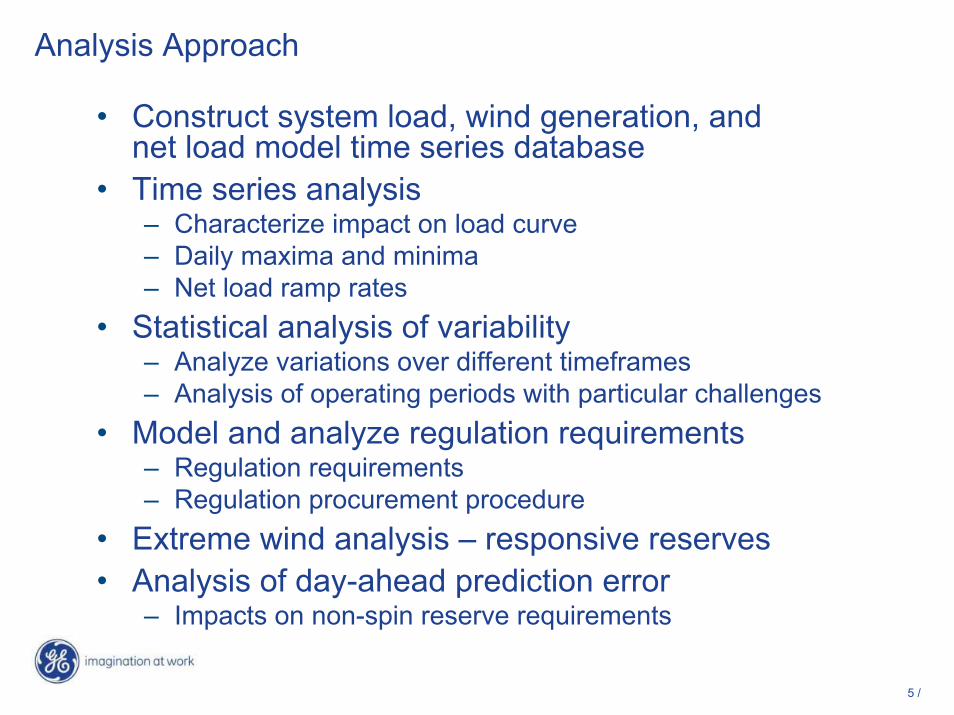
Analysis Approach

• Construct system load, wind generation, and net load model time series database

• Time series analysis– Characterize impact on load curve– Daily maxima and minima– Net load ramp rates

• Statistical analysis of variability– Analyze variations over different timeframes– Analysis of operating periods with particular challenges

• Model and analyze regulation requirements– Regulation requirements– Regulation procurement procedure

• Extreme wind analysis – responsive reserves • Analysis of day-ahead prediction error

– Impacts on non-spin reserve requirements

6 /

Net Load Model

• Two years of data used– More accuracy and consistency– Two consecutive years needed later in Phase 2 for testing A/S

methodology• Essential for system load and wind generation data to be for consistent

time period– Common factors affect both wind and load

• System one-minute load data– Based on 2005 and 2006 ERCOT historical recordings– 2006 data scaled up to achieve average load (energy) consistent

with 2008 ERCOT predictions – “Study Year”– 2005 data scaled by the same factor – “Previous Year”– Scale factor = 1.037, computed from the average ratio of forecasted

2008 load to 2006 actual load across all hours – Day-ahead load forecasts provided by ERCOT

7 /

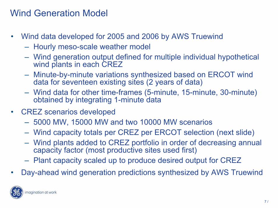
Wind Generation Model

• Wind data developed for 2005 and 2006 by AWS Truewind– Hourly meso-scale weather model– Wind generation output defined for multiple individual hypothetical

wind plants in each CREZ– Minute-by-minute variations synthesized based on ERCOT wind

data for seventeen existing sites (2 years of data)– Wind data for other time-frames (5-minute, 15-minute, 30-minute)

obtained by integrating 1-minute data• CREZ scenarios developed

– 5000 MW, 15000 MW and two 10000 MW scenarios – Wind capacity totals per CREZ per ERCOT selection (next slide)– Wind plants added to CREZ portfolio in order of decreasing annual

capacity factor (most productive sites used first)– Plant capacity scaled up to produce desired output for CREZ

• Day-ahead wind generation predictions synthesized by AWS Truewind

8 /

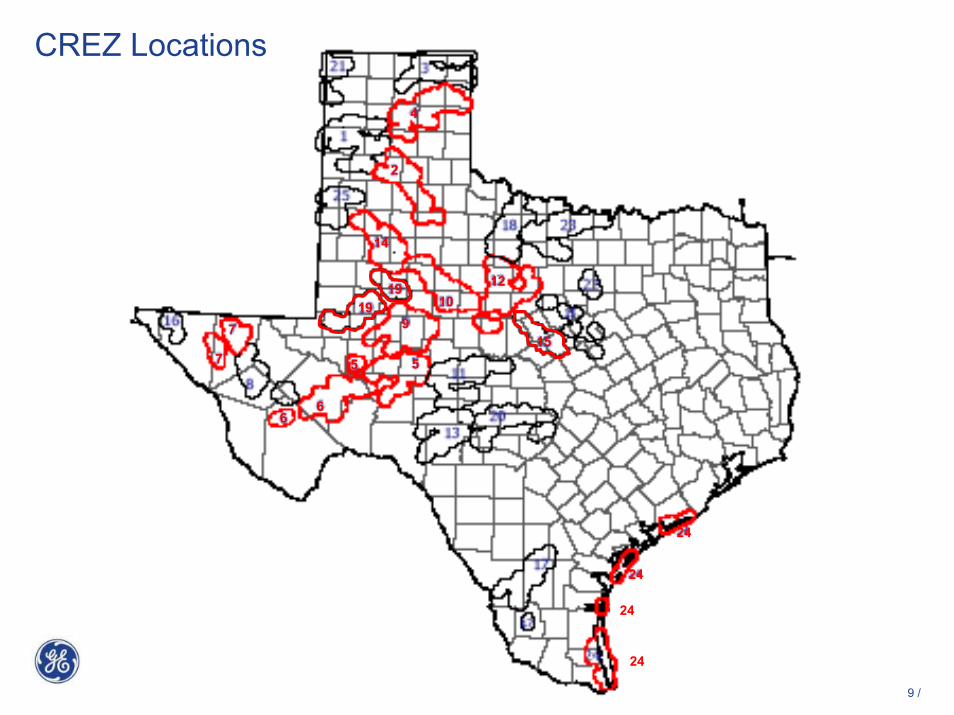
CREZ Scenarios

Wind Development Scenario CREZ Zone 5000 MW 10,000 MW (1) 10,000 MW (2) 15,000 MW

none 120 120 120 120 2 60 1,560 1,560 2,340 4 0 1,500 0 0 5 355 1,355 1,355 1,355 6 400.5 400.5 400.5 1,278.3 7 65 65 65 97.5 9 814 1,314 1,314 1,971

10 2,464.5 2,964.5 2,964.5 4,446.8 12 400 400 400 600 14 160 160 160 240 15 60 60 60 90 19 101 101 101 211.5 24 0 0 1,500 2,250

Difference in two 10,000 MW scenarios is that the second has 1,500 MW of wind generation in the Gulf coastal area, substituting for a like amount in the panhandle

9 /

1919

910

12

1555

66

7

7

14

4

2

24

24

24

24

CREZ Locations

10 /

Time Series Plots and Daily Profiles

11 /

In this next set of slides, we will show how wind and load interact to create the net load curves.

Key issues are:• Impacts on net load peaks and valleys• Increases in ramp rates• Common factors affecting wind and load

12 /

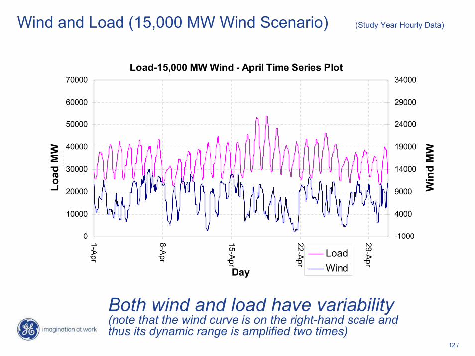
Wind and Load (15,000 MW Wind Scenario) (Study Year Hourly Data)

Load-15,000 MW Wind - April Time Series Plot

0

10000

20000

30000

40000

50000

60000

70000

1-Apr

8-Apr

15-Apr

22-Apr

29-Apr

Day

MW

-1000

4000

9000

14000

19000

24000

29000

34000

LoadWind

Load

MW

Win

d M

W

Both wind and load have variability(note that the wind curve is on the right-hand scale and thus its dynamic range is amplified two times)

13 /

Average April Daily Load and Wind Profile (15,000 MW Wind)2008 Load-15,000 MW Wind - April Daily Profile

20000

25000

30000

35000

40000

45000

50000

55000

60000

65000

0 4 8 12 16 20 24Hour

MW

0

1000

2000

3000

4000

5000

6000

7000

8000

9000

LoadWind

(Study Year Hourly Data)

Load

MW

Win

d M

W

• Wind is generally out-of-phase with load• Sharp drop in wind in the morning when load is rising• Sharp wind increase when load drops sharply in the

evening

14 /

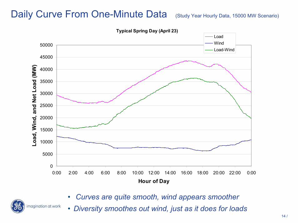
Daily Curve From One-Minute Data (Study Year Hourly Data, 15000 MW Scenario)

Typical Spring Day (April 23)

0

5000

10000

15000

20000

25000

30000

35000

40000

45000

50000

0:00 2:00 4:00 6:00 8:00 10:00 12:00 14:00 16:00 18:00 20:00 22:00 0:00

Hour of Day

Load

, Win

d, a

nd N

et L

oad

(MW

)LoadWindLoad-Wind

• Curves are quite smooth, wind appears smoother• Diversity smoothes out wind, just as it does for loads

15 /

Net Load (15,000 MW Wind Scenario) (Study Year Hourly Data)

Load-15,000 MW Wind - April Time Series Plot

0

10000

20000

30000

40000

50000

60000

70000

1-Apr

8-Apr

15-Apr

22-Apr

29-Apr

Day

MW

WindLoadNet Load

• Load peaks are reduced, some days more than others• Valleys are greatly deepened

16 /

Net Load Comparisons – One January Week (Study Year Hourly Data)

0

5000

10000

15000

20000

25000

30000

35000

40000

45000

50000

15-Jan

16-Jan

17-Jan

18-Jan

19-Jan

20-Jan

21-Jan

22-Jan

Day

MW

Load5,000 MW10,000 MW (1)10,000 MW (2)15,000 MW

Increased ramp rate

Increased daily range

• Curve shape is relatively similar for all scenarios• Peak-to-valley change increases with wind generation• Result is ramp rates increasing with more wind

17 /

Net Load Comparisons – One April Week (Study Year Data)

10000

15000

20000

25000

30000

35000

40000

45000

50000

55000

60000

13-Apr

14-Apr

15-Apr

16-Apr

17-Apr

18-Apr

19-Apr

20-Apr

Day

MW

Load5,000 MW10,000 MW (1)10,000 MW (2)15,000 MW

Thursday Wednesday

0

10000

20000

30000

40000

50000

MW

Load

Wind (15 GW Scenario)

Net Load

Load dip

Wind spike

• Perturbation in both wind and load at the same time, likely from common source (e.g., cold front)

• Valid analysis requires synchronized load and wind data

18 /

In summary:

• Both wind and load are variable– Daily wind generation cycle is generally out-of-phase

with load– Shorter term variations tend to be less correlated

• Common factors affect both wind and load– Wind impacts cannot be correctly considered

independently of load behavior

19 /

Time of Year (Seasonal) Analysis

20 /

In the next series of slides, time periods with critical operating situations are identified and the impacts of wind are illustrated by time series plots (all with the 15000 MW scenario to more clearly demonstrate wind impacts)Critical situations include: • Maximum system load• Minimum net load• Maximum net load• Most variable day

21 /

Profiles of Daily Average Load and Net Load and 1-Hour Deltas(Study Year Data, 15000 MW Scenario)

-18000

-12000

-6000

0

6000

12000

18000

24000

30000

36000

42000

48000

54000

Load

and

Net

Loa

d (M

W)

-8000

-5000

-2000

1000

4000

7000

10000

13000

16000

19000

22000

25000

28000

Max

/Min

of O

ne-H

our D

elta

s (M

W)

LoadLoad-WindMax Load-Wind 1Hr DeltasMin Load-Wind 1Hr Deltas

Jan Feb Mar Apr May Jun Jul Aug Sep Oct Nov Dec

Winter

Spring

Summer

Fall

Largest Net-Load Delta Day May 8th

Peak Load Day August 17th

Min Load Day Mar 27th

These are the maximum and minimum deltas (derivative of hourly load curve) for each day

These are average loads and net loads for each day (equal to daily MWh/24)

• Basis for selection of key dates for further illustration and analysis

22 /

Largest Net-Load Delta Day - Profiles and Deltas (Study Year Data, 15000 MW Scenario)

Largest Net-Load Delta Day (May 8)

0

5000

10000

15000

20000

25000

30000

35000

40000

45000

50000

1 2 3 4 5 6 7 8 9 10 11 12 13 14 15 16 17 18 19 20 21 22 23 24

Hour of Day

Load

and

Net

Loa

d (M

W)

-8000

-6000

-4000

-2000

0

2000

4000

6000

8000

10000

12000LoadLoad-WindWind (15000 MW)Load 1Hr DeltasLoad-Wind 1Hr Deltas

4-hr peak shift

~5900 MW

~6300 MW

~5000 MW

One

-Hou

r Del

tas

(MW

)

• Wind drop in evening before load drop causes a late peak in net load, with resulting increases in ramp rates

23 /

Most Variable* Day - Profiles and 1-Hour Deltas (Study Year Data, 15000 MW Scenario)

Most Variable Net Load Day (July 12)

0

7000

14000

21000

28000

35000

42000

49000

56000

63000

70000

1 2 3 4 5 6 7 8 9 10 11 12 13 14 15 16 17 18 19 20 21 22 23 24

Hour of Day

Load

and

Net

Loa

d (M

W)

-8000

-6000

-4000

-2000

0

2000

4000

6000

8000

10000

12000

One

-Hou

r Del

tas

(MW

)

LoadLoad-WindWind (15000 MW)Load 1Hr DeltasLoad-Wind 1Hr Deltas

34350 MW rise over 12 hours (~2900 MW/Hr)

27560 MW drop over 8 hours (~3500 MW/Hr)

* Largest net-load sigma

• Anti-correlation of diurnal load and wind curves cause severe morning and evening ramps

24 /

In summary:• Wind has the greatest impact on hour-to-hour net load

variation in the late spring and summer– Strong coincidence of wind drop-off with

morning load pickup– Strong coincidence of wind pickup with evening load

drop-off– Larger day vs. night net load swing results in greater

ramp rates • Variations in the winter and early spring may be more

operationally significant, however, due to low net load levels• Net load peaks can be shifted to unusual times of day by

wind changes with high penetration

25 /

Net-Load Variability for Various Timeframes

26 /

Statistical analysis of the load and net load variability is shown in the next series of slides, for different timeframesSome explanations and points to consider:• Deltas are the changes in average net load

for successive periods – (1, 5, 15, and 60 minutes considered in this study)

• Average deltas over a day or longer period are inherently near zero, so the standard deviation of the deltas are used as a measure of variability

• Deltas include both the effects of longer-cycle ramping as well as random “jitter”

27 /

One-Minute Load-Wind Variability (Study Year Data, 15000 MW Scenario)

-39.2 / 38.1-33.6 / 33.0Mean(-/+ Deltas)

491.6

-513.7

43.22

Load-alone (MW)

-552.6Min. Delta

Max. Delta

Sigma (Delta)

538.3

49.67

With Wind (MW)

Statistical Summary

0

10000

20000

30000

40000

50000

60000

70000

80000

90000

< -240

-240 – -224

-224 – -208

-208 – -192

-192 – -176

-176 – -160

-160 – -144

-144 – -128

-128 – -112

-112 – -96

-96 – -80

-80 – -64

-64 – -48

-48 – -32

-32 – -16

-16 – 0

0 – 16

16 – 32

32 – 48

48 – 64

64 – 80

80 – 96

96 – 112

112 – 128

128 – 144

144 – 160

160 – 176

176 – 192

192 – 208

208 – 224

224 – 240

> 240

MW

Num

ber o

f One

-Min

ute

Perio

ds Load - WindLoad

Greatest difference between net load and load alone is in the downward change direction

111 / 13979 / 87105 / 129>µ ± 6σ (−/+)

3593 / 27691517 / 12391711 / 1435>µ ± 3σ (−/+)

571 / 551247 / 297338 / 391>µ ± 4σ (−/+)

9277 / 74084604 / 35474696 / 3805>µ ± 2.5σ (−/+)

1.61%

147 / 203

Load-alone (Delta-MW)σ = 43.22

3.17%1.55%% > 2.5σ

>µ ± 5σ (−/+) 175 / 225117 / 159

With Wind(Delta-MW)Using load σ

With Wind (Delta-MW)σ = 49.67

Extreme 1-Minute Deltas

1-minute standard deviation (σ ) increases by 14.9%Maximum 1-minute rise increases by 46.4 MWMaximum 1-minute drop increases by 38.9 MWNumber of 1-minute deltas greater than 2.5 (load)σincreases 96%

28 /

Hourly Load-Wind Variability (Study Year Data, 15000 MW Scenario)

0

200

400

600

800

1000

1200

< -7000-7000 – -6500-6500 – -6000-6000 – -5500-5500 – -5000-5000 – -4500-4500 – -4000-4000 – -3500-3500 – -3000-3000 – -2500-2500 – -2000-2000 – -1500-1500 – -1000-1000 – -500-500 – 00 – 500500 – 10001000 – 15001500 – 20002000 – 25002500 – 30003000 – 35003500 – 40004000 – 45004500 – 50005000 – 55005500 – 60006000 – 65006500 – 7000> 7000

MW

No.

1-H

our P

erio

ds

Load - WindLoad

Again, the downward variations are most changed

-1741 / 1677-1366 / 1425Mean(-/+ Deltas)

5203

-4838

1758

Load-alone (MW)

-7507Min. Delta

Max. Delta

Sigma (Delta)

6861

2159

With Wind (MW)

78 / 366 / 50 / 0>µ ± 3σ (−/+)

224 / 1616 / 2643 / 26>µ ± 2.5σ (−/+)

0.79%

0 / 0

Load-alone (Delta-MW)σ = 1758

4.39%0.37%% > 2.5σ

>µ ± 4σ (−/+) 1 / 00 / 0


With Wind (Delta-MW)σ = 2159

Extreme 1-Hour Deltas

1-hr standard deviation (σ ) increases by 22.8% Maximum 1-hour rise increases by 1658 MWMaximum 1-hour drop increases by 2669 MWNumber of 1-hr deltas greater than 2.5 (load)σincreases 458%

29 /

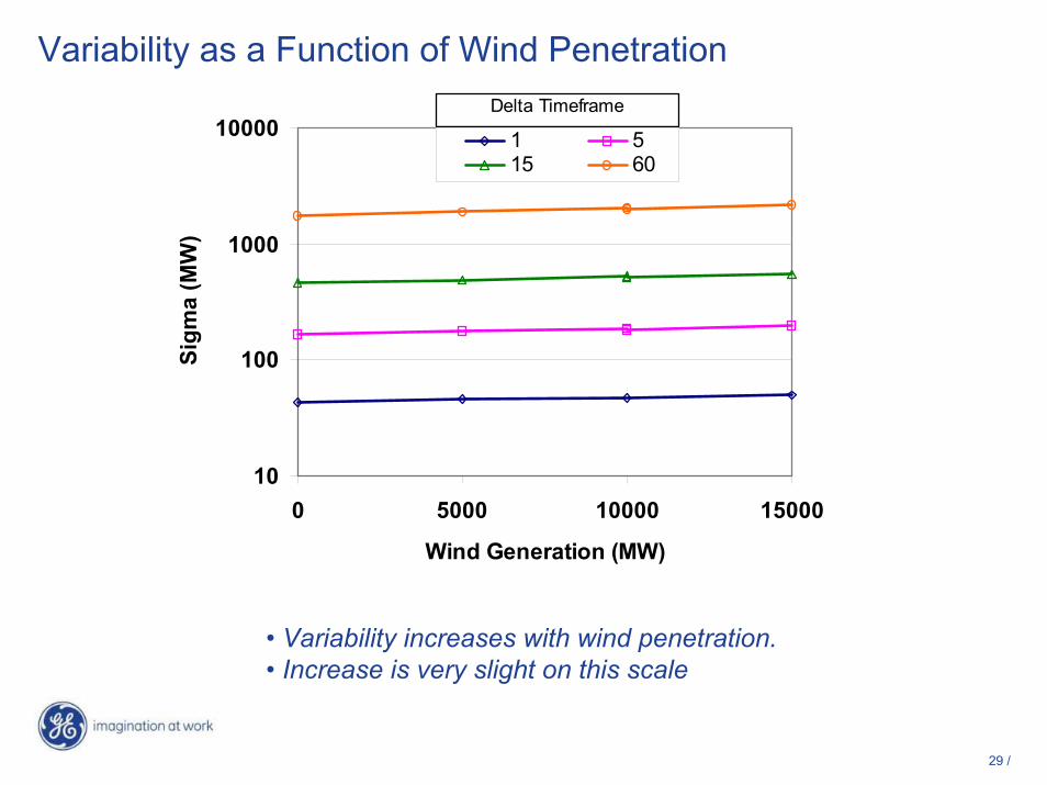
Variability as a Function of Wind Penetration

10

100

1000

10000

0 5000 10000 15000

Wind Generation (MW)

Sigm

a (M

W)

1 515 60

Delta Timeframe

• Variability increases with wind penetration. • Increase is very slight on this scale

30 /

Normalized Variability as a Function of Wind Penetration

10

15

2025

30

35

4045

50

55

0 5000 10000 15000

Wind Generation (MW)

Nor

mal

ized

Sig

ma

(MW

/min

) 1 5 15 60

Delta Timeframe

• Sigmas normalized in terms of MW/min (e.g., σ5 / 5)• Increase is linear, but with a shallow slope

31 /

Normalized Sigma as a Function of Timespan

0

10

20

30

40

50

60

1 10 100

Timespan (minutes)

Nor

mal

ized

Sig

ma

(MW

/min

)

Load Only5,000 MW10,000 MW10,000 MW15,000 MW

`

• There is a baseline of variability that is a function of the longer-term load cycle.

• An incremental amount of variation appears at the shortest timeframes (1 & 5 min.)

32 /

Increase in Variability Relative to Time Span

For all wind scenarios, the relative increase in variability (sigma), relative to sigma of load alone, becomes more significant for longer time windows

0%

5%

10%

15%

20%

25%

1 10 100

Timespan (minutes)

% In

crea

se in

Var

iabi

lity

5,000 MW 10,000 MW 10,000 MW 15,000 MW

33 /

In summary:• Variations over timespans of 10+ minutes are primarily due

to load cycle• Shorter timespans have an incremental component due to

random “noise” variations• Wind causes a slight, linear increase in period-to-period

variability over all timespans• Impact is somewhat more significant for longer timespans

– I.e., wind adds to variability primarily due to creating larger daily net load swings

– Addition to the random “noise” is less significant• Small differences in statistical metrics between “study year”

(based on 2006) and “previous year” (based on 2005) indicate stability of results

34 /

Variability at Different Load Levels

35 /

The ability of the system to accommodate net load variations is greatly a function of the absolute net load level.

System maneuverability tends to increase with the generation level because:• Variations of a given magnitude are larger in

proportion to the committed generators• Units lower on the dispatch stack tend to be

base load units that are less maneuverable

The following slides correlate variability with load level

36 /

Wind Duration and Penetration (15000 MW) (Study Year Data)

0

2500

5000

7500

10000

12500

15000

0 876 1752 2628 3504 4380 5256 6132 7008 7884 8760

Hours of Year

Tota

l Win

d O

utpu

t(MW

)

0%

10%

20%

30%

40%

50%

60%

Win

d Pe

netr

atio

n (%

)

Total Wind (MW)

Penetration (%)

Note: Data for these curves were independently sorted

Wind generation is above 75% of installed capacity only 10% of the year

Median instantaneous penetration is only 16%, compared to 23% on a capacity basis

Wind Scenario Max Instantaneous Penetration

5000 21%10000 (1) 39%10000 (2) 39%15000 57%

37 /

Load and Net Load Variability by Load Level (Study Year Hourly Data, 15000 MW Scenario)(Average +/- x*sigma, Minimum, Maximum)

LoadLoad-Wind

-8000

-6000

-4000

-2000

0

2000

4000

6000

8000

MW

1 2 3 4 5 6 7 8 9 10Load Decile

Mean + Sigma

Mean - 2.5*Sigma

Mean - Sigma

Mean + 2.5*SigmaMax

Min

Very little impact on variability at very high load levels

• Variability is changed little at lower loads• Same variability, but with fewer dispatchable generators

38 /

Net Load Duration Curves for Various Wind Scenarios (Study Year Data)

0

10000

20000

30000

40000

50000

60000

70000

0 876 1752 2628 3504 4380 5256 6132 7008 7884 8760

Hours of Year

Net

Loa

d (M

W)

Load-AloneLoad-5000 MWLoad-10000 MW(1)Load-10000 MW(2)Load-15000 MWMin Load (22426 MW)

Low net load periods

Min Load 22426 MW



• Net loads below current minimum load may be a real operational challenge

• Average wind output is double during low net-load hours

39 /

Net Load Duration Curves for Low Load Periods (Study Year Data)

8000

12000

16000

20000

24000

28000

32000

6700 6900 7100 7300 7500 7700 7900 8100 8300 8500 8700

Hours of Year

Net

Loa

d (M

W)

Load-AloneLoad-5000 MWLoad-10000 MW(1)Load-10000 MW(2)Load-15000 MWMin Load (22426 MW)

1945 hrs (35.7% of Wind Energy)

1141 hrs (21.4%E)

470 hrs (9.7%E)

1209 hrs (23.3%E)

8760

Wind energy lost if wind is curtailed to hold min net load same (5,000 MW scenario)

• There are inherent tradeoffs between costs of generation flexibility and energy lost to curtailment

Curtailment to hold current minimum for 15 GW of wind results in excessive energy loss

40 /

In summary:• In general, variability is relatively constant over the range of

load levels• Wind contribution to variability is also relatively constant• Net loads can be driven to low levels with large wind

capacity– Instantaneous penetration reaches 55% with 15,000 MW

of wind and 2008 load levels• It is not feasible to maintain the same minimum load levels

Ability of the ERCOT system to meet ramping requirements will be specifically studied in Phase 2

41 /

Time of Day Variability Analysis

42 /

The next slides examine how load variability varies over the hours of the day for different seasons

43 /

April, Hourly Load and Net Load Deltas (Study Year Data, 15000 MW Scenario)

(Avg. +/- sigma, Minimum, Maximum)

0 1 2 3 4 5 6 7 8 9 10 11 12 13 14 15 16 17 18 19 20 21 22 23 24 250

6000

12000

18000

24000

30000

36000

42000

48000

-8000

-6000

-4000

-2000

0

2000

4000

6000

8000

-8000

-6000

-4000

-2000

0

2000

4000

6000

8000

Hour of Day

Load

and

Net

Loa

d D

elta

(MW

)

Tota

l Loa

d (M

W)

Wind is a large contributor to ramping requirements during morning load rise and evening load drop off in the spring

5900 MW/hr drop

5700 MW/hr rise

Load DeltasLoad-Wind DeltasTotal LoadLoad-Wind

44 /

July, Hourly Load and Net Load Deltas (Study Year Data, 15000 MW Scenario)


0 1 2 3 4 5 6 7 8 9 10 11 12 13 14 15 16 17 18 19 20 21 22 23 24 250

7500

15000

22500

30000

37500

45000

52500

60000

-8000

-6000

-4000

-2000

0

2000

4000

6000

8000

-8000

-6000

-4000

-2000

0

2000

4000

6000

8000

Hour of Day

Load

and

Net

Loa

d D

elta

(MW

)

Load

and

Net

Loa

d (M

W)

In summer, wind makes the largest impact during the early morning load rise and evening load drop off

6650 MW/hr rise

6400 MW/hr drop

Load DeltasLoad-Wind DeltasTotal LoadLoad-Wind

45 /

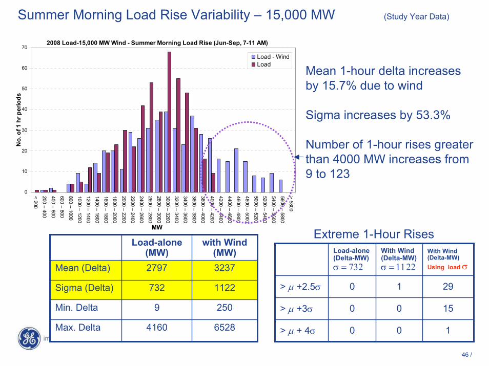
Summer Morning Load Rise PeriodJune – September

7 – 11 AM

46 /

Summer Morning Load Rise Variability – 15,000 MW (Study Year Data)

32372797Mean (Delta)

2509Min. Delta

Max. Delta

Sigma (Delta)

65284160

1122732

with Wind (MW)

Load-alone (MW)

2008 Load-15,000 MW Wind - Summer Morning Load Rise (Jun-Sep, 7-11 AM)

0

10

20

30

40

50

60

70

< 200

200 – 400

400 – 600

600 – 800

800 – 1000

1000 – 1200

1200 – 1400

1400 – 1600

1600 – 1800

1800 – 2000

2000 – 2200

2200 – 2400

2400 – 2600

2600 – 2800

2800 – 3000

3000 – 3200

3200 – 3400

3400 – 3600

3600 – 3800

3800 – 4000

4000 – 4200

4200 – 4400

4400 – 4600

4600 – 4800

4800 – 5000

5000 – 5200

5200 – 5400

5400 – 5600

5600 – 5800

> 5800

MW

No.

of 1

hr p

erio

ds

Load - WindLoad

Mean 1-hour delta increases by 15.7% due to wind

Sigma increases by 53.3%

Number of 1-hour rises greater than 4000 MW increases from 9 to 123

2910> µ +2.5σ

0

0


10> µ + 4σ

> µ +3σ 150



Extreme 1-Hour Rises

47 /

Summer Morning Load Rise Variability (Study Year Data)

Summer Morning Load Rise

0

1000

2000

3000

4000

5000

6000

7000

0 5000 10000 15000 20000

Wind Penetration (MW)

MW

µ

σ

µ + 2.5 σExtreme

• Extrema increase more quickly with additional wind generation than mean + 2.5 s.d.

• Distribution is less characterized by a normal distribution; more outliers

48 /

Winter Afternoon Load Rise PeriodNovember – February

4 – 6 PM

49 /

Winter Afternoon Load Rise Variability (Study Year Data)

15731517Mean (Delta)

-2768-886Min. Delta

Max. Delta

Sigma (Delta)

68613678

1556866

with Wind (MW)

Load-alone (MW)

2008 Load-15,000 MW Wind - Winter Afternoon Load Rise (Nov-Feb, 4-6PM)

0

5

10

15

20

25

30

35

< -2800-2800 – -2700-2700 – -2400-2400 – -2100-2100 – -1800

-1800 – -1500-1500 – -1200-1200 – -900-900 – -600

-600 – -300-300 – 00 – 300300 – 600600 – 900

900 – 12001200 – 15001500 – 18001800 – 2100

2100 – 24002400 – 27002700 – 30003000 – 33003300 – 3600

3600 – 39003900 – 42004200 – 45004500 – 4800

4800 – 51005100 – 54005400 – 57005700 – 6000> 6000

MW

No.

of 1

hr p

erio

ds

Load - WindLoad

More outliers, both directions Mean 1-hour delta increases by

3.7% due to wind

Sigma increases by 79.7%

Number of 1-hour rises greater than 3000 MW increases from 11 to 36

2250> µ +2.5σ

0

0


70> µ + 4σ

> µ +3σ 144



Extreme 1-Hour Rises

50 /

• Wind variability increases linearly with penetration– 1-hour sigma increases by 23% with 15,000 MW of wind– Greater variability and extreme ramps observed during

certain morning, afternoon and evening periods– Greater net load variability in the spring and summer

• The more significant impact is that minimum net loads are greatly reduced– Greater relative variability at light load– Less system responsiveness

• Wind impact on variability is primarily due to multi-hour cycles, increment due to “noise” is small

• Wind has incremental impact on average and extreme errors, especially during early mornings and afternoons in winter & spring– On average, net load is nearly as predictable as load alone

Variability Analysis Summary

51 /

Extreme Weather Conditions

Impact on Ancillary Services

52 /

Impact of Extreme Weather Conditions

• ERCOT’s current “extreme” weather conditions are largely defined by temperature … – Regulation reserves may be increased by a

factor of two– Responsive reserves and non-spinning reserves

may be procured• With large amounts of wind, other weather

conditions may create abnormal net load deviations– Investigate most severe events in wind and Net-

Load– Develop modified procedures or requirements for

identifying and responding to the ancillary service needs driven by extreme weather.

53 /

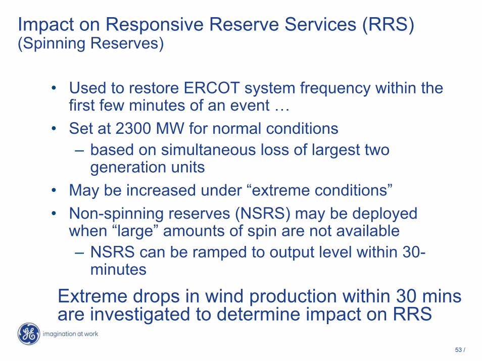
Impact on Responsive Reserve Services (RRS) (Spinning Reserves)

• Used to restore ERCOT system frequency within the first few minutes of an event …

• Set at 2300 MW for normal conditions– based on simultaneous loss of largest two

generation units• May be increased under “extreme conditions”• Non-spinning reserves (NSRS) may be deployed

when “large” amounts of spin are not available– NSRS can be ramped to output level within 30-

minutes

Extreme drops in wind production within 30 minsare investigated to determine impact on RRS

54 /

In this next set of slides, we will show:• AWST analysis of ramp events in existing wind

– Causes, frequency and predictability– Implications for wind scenarios

• Probability of “large” wind transitions/ramp events• Impact of diversity on wind ramp events• Distribution, timing and magnitude of events• Implications for RRS requirements

55 /

Analysis of West Texas Wind Plant Ramp EventsTo identify and classify events, AWS Truewind:• Examined two years of one-minute plant output data provided by

ERCOT– Identified 30-minute periods with aggregate wind generation

changes > 200 MWTotal 976 MW rated capacity for plants in analysisObvious cases of non-weather curtailments and shutdowns excluded

– Examined available meteorological records for the periods – Categorized the events by meteorological causes

• Analyzed significant 2005-2006 weather events identified by ERCOT, determined those were associated with large changes in wind generation

• Analyzed the event of 24 February 2007 and established the causefor the decrease in energy production.

From the results, AWS Truewind estimated the maximum likely change in a 30-minute period for the 15,000 MW scenario

56 /

Meteorological Causes of Wind Ramp-Up Events• Frontal system/trough/dry line

– Density fronts or air mass discontinuities – Accompanying fall/rise pressure couplet, results in rapid wind-

speed change, – Mostly move west to east or northwest to southeast – Up to 1000 km long and 100-200 km wide– Propagate at over 15 m/s (34 mph)

• Convection-induced outflow or gust fronts – Occur on the mesoscale (tens to hundreds of square km) – Usually propagate radially outward from thunderstorm clusters – Propogation speeds in excess of 25 m/s

• Low-level jet (LLJ) – Occur regularly year-round in the Southern Great Plains– Two types:

1) Nocturnal LLJ – maximum at 5 AM2) Pre-frontal LLJ – ahead of cold front

57 /

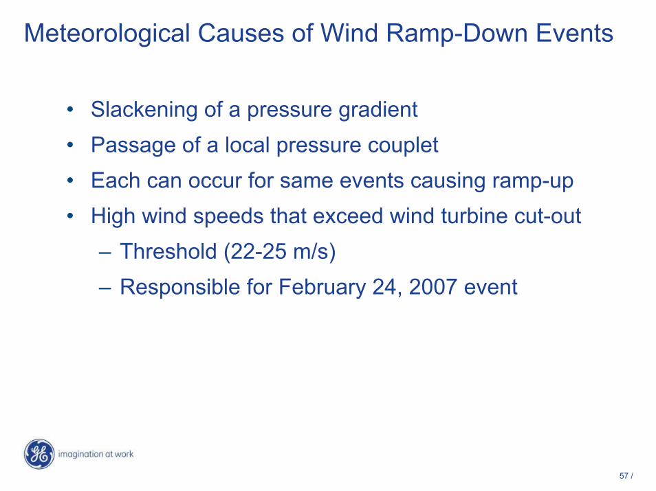
Meteorological Causes of Wind Ramp-Down Events

• Slackening of a pressure gradient • Passage of a local pressure couplet • Each can occur for same events causing ramp-up• High wind speeds that exceed wind turbine cut-out

– Threshold (22-25 m/s) – Responsible for February 24, 2007 event

58 /

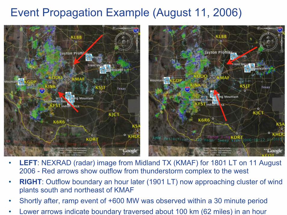
Event Propagation Example (August 11, 2006)

• LEFT: NEXRAD (radar) image from Midland TX (KMAF) for 1801 LT on 11 August 2006 - Red arrows show outflow from thunderstorm complex to the west

• RIGHT: Outflow boundary an hour later (1901 LT) now approaching cluster of wind plants south and northeast of KMAF

• Shortly after, ramp event of +600 MW was observed within a 30 minute period • Lower arrows indicate boundary traversed about 100 km (62 miles) in an hour

59 /

Extreme Wind Events* in Existing Data (2006)**

* 200 MW excursion within 30 minutes

** Based on approximately 976 MW of installed capacity

60 /

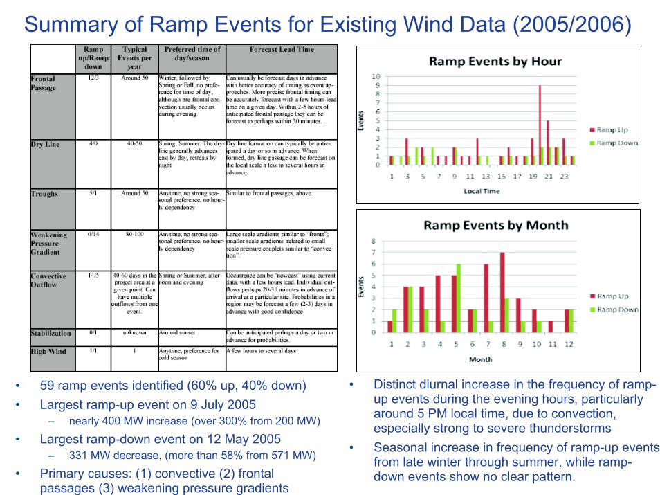
Summary of Ramp Events for Existing Wind Data (2005/2006)

• 59 ramp events identified (60% up, 40% down)• Largest ramp-up event on 9 July 2005

– nearly 400 MW increase (over 300% from 200 MW)

• Largest ramp-down event on 12 May 2005 – 331 MW decrease, (more than 58% from 571 MW)

• Primary causes: (1) convective (2) frontal passages (3) weakening pressure gradients

• Distinct diurnal increase in the frequency of ramp-up events during the evening hours, particularly around 5 PM local time, due to convection, especially strong to severe thunderstorms

• Seasonal increase in frequency of ramp-up events from late winter through summer, while ramp-down events show no clear pattern.

61 /

Ramp Event Case Study (December 28, 2006)

• Weak gradient ahead of cold front– An area of weak pressure gradient moves

eastward across west-central Texas between 14:00 and 15:00 LST

– Since wind speed is proportional to the pressure gradient, there is a significant reduction in wind power output and wind speed as this feature passes

– The drop in wind speed is most notable at Fort Stockton (KFST), Lubbock (KLBB) and Odessa (KODO)

– There is a secondary drop in power output around 16:00 LST as winds continue to diminish (to below the cut-in value of 4 m/s at the stations)

• Frontal passage– Following the weak pressure field, a

stronger gradient moves into the area after the frontal passage (approximately 15:00 –16:00 LST)

– Wind speeds and output increase rapidly by 18:00

– Plant output, which had decreased to about 100 MW (or 10% of the rated capacity), then rapidly rose as wind speeds rose above the cut-in value.

62 /

Ramp Event Case Study (February 24, 2007)• Strong upper-level storm system passed over

northern New Mexico and the panhandle of Texas substantially tightening the pressure gradients over west Texas, resulting in strong to severe winds along a straight line across much of the area

– 8 AM - high wind speeds seen by most wind projects, maximum wind gust reported was 94 mph

– 9 AM - aggregate output increased from just over 1100 MW to nearly 2000 MW (rated capacity)

– 10 AM - sustained winds exceeded 25 m/s (55 mph) output at most wind farms, output declined as turbine-cutoff threshold reached

– 11 AM - most intense pressure gradients and winds moved eastward, wind speeds relaxed, turbines resumed power production, resulting in a gradual increase in total output to pre-event levels

• Total drop in plant output was more than 1500 MW over a 90 minute period

• Most rapid declines occurred at the Horse Hollow interconnections

• Largest 30-minute drop of 450 MW (between 1104 and 1134 LST) represents about 22.5% of the plant rated capacity

• The event was unusual both in the magnitude of the 90-minute drop and the large geographic area affected

• Arrival of such fronts is generally forecastable, several hours ahead within a 30-minute window

63 /

February 24, 2007, 1400 Local Standard Time

64 /

Probability and Predictability of Ramp Events• Frontal passages/troughs/dry lines of any severity

occur every 3-5 days during cold season, and every 5-7 days during warm season– Fast ramp-up events (as defined for 2005/2006 existing data)

likely to occur 20 times/year or every 2-3 weeks– Fast down-ramps likely to occur once every 2 months

• Convective events occur with varying frequency– Number of severe thunderstorms (winds over 29 m/s) in

ERCOT territory over last 10 years varies from 32 in 2000 to 134 in 2003

• All weather phenomena causing ramp events can be forecasted– Lead time and accuracy varies considerably– Frontal passages (winter) can be forecasted several days in

advance with limited accuracy and timing, but to within a 30-minute window several hours in advance

– Severe thunderstorms (summer) more difficult to forecast, better for active periods – average lead time in West Texas is 20 minutes, 70-85% accuracy, but only 30-40% dependability

65 /

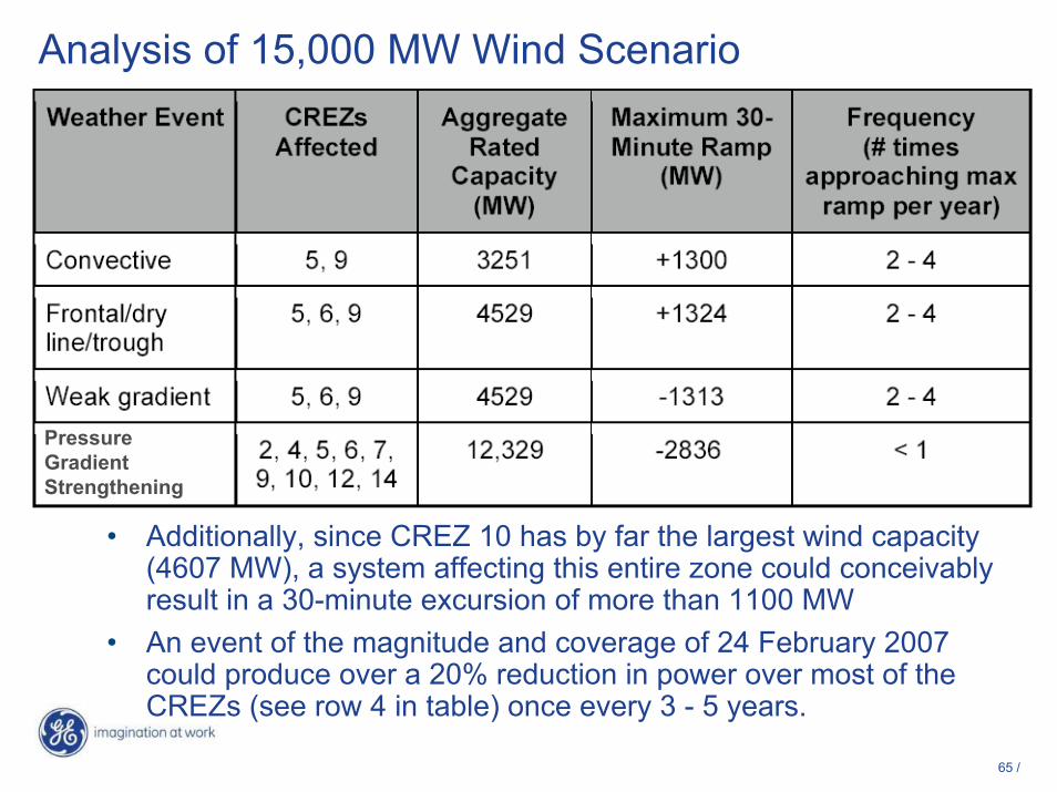
Analysis of 15,000 MW Wind Scenario

Pressure Gradient Strengthening

• Additionally, since CREZ 10 has by far the largest wind capacity(4607 MW), a system affecting this entire zone could conceivablyresult in a 30-minute excursion of more than 1100 MW

• An event of the magnitude and coverage of 24 February 2007 could produce over a 20% reduction in power over most of theCREZs (see row 4 in table) once every 3 - 5 years.

66 /

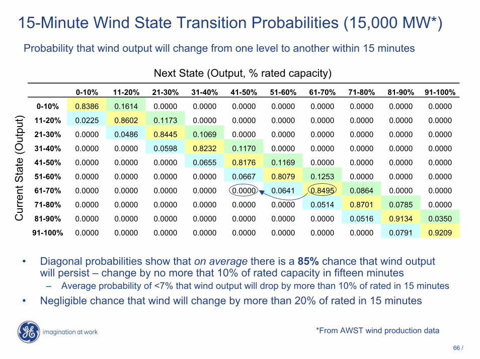
15-Minute Wind State Transition Probabilities (15,000 MW*)Probability that wind output will change from one level to another within 15 minutes

Next State (Output, % rated capacity)

Cur

rent

Sta

te (O

utpu

t)

0-10% 11-20% 21-30% 31-40% 41-50% 51-60% 61-70% 71-80% 81-90% 91-100%

0-10% 0.8386 0.1614 0.0000 0.0000 0.0000 0.0000 0.0000 0.0000 0.0000 0.0000

11-20% 0.0225 0.8602 0.1173 0.0000 0.0000 0.0000 0.0000 0.0000 0.0000 0.0000

21-30% 0.0000 0.0486 0.8445 0.1069 0.0000 0.0000 0.0000 0.0000 0.0000 0.0000

31-40% 0.0000 0.0000 0.0598 0.8232 0.1170 0.0000 0.0000 0.0000 0.0000 0.0000

41-50% 0.0000 0.0000 0.0000 0.0655 0.8176 0.1169 0.0000 0.0000 0.0000 0.0000

51-60% 0.0000 0.0000 0.0000 0.0000 0.0667 0.8079 0.1253 0.0000 0.0000 0.0000

61-70% 0.0000 0.0000 0.0000 0.0000 0.0000 0.0641 0.8495 0.0864 0.0000 0.0000

71-80% 0.0000 0.0000 0.0000 0.0000 0.0000 0.0000 0.0514 0.8701 0.0785 0.0000

81-90% 0.0000 0.0000 0.0000 0.0000 0.0000 0.0000 0.0000 0.0516 0.9134 0.0350

91-100% 0.0000 0.0000 0.0000 0.0000 0.0000 0.0000 0.0000 0.0000 0.0791 0.9209

• Diagonal probabilities show that on average there is a 85% chance that wind output will persist – change by no more that 10% of rated capacity in fifteen minutes

– Average probability of <7% that wind output will drop by more than 10% of rated in 15 minutes• Negligible chance that wind will change by more than 20% of rated in 15 minutes

*From AWST wind production data

67 /

30-Minute Wind State Transition Probabilities (15,000 MW*)Probability that wind output will change from one level to another within 30 minutes


Cur

rent

Sta

te (O

utpu

t)

0-10% 11-20% 21-30% 31-40% 41-50% 51-60% 61-70% 71-80% 81-90% 91-100%

0-10% 0.8139 0.1861 0.0000 0.0000 0.0000 0.0000 0.0000 0.0000 0.0000 0.0000

11-20% 0.0199 0.8094 0.1707 0.0000 0.0000 0.0000 0.0000 0.0000 0.0000 0.0000

21-30% 0.0000 0.0595 0.7698 0.1699 0.0008 0.0000 0.0000 0.0000 0.0000 0.0000

31-40% 0.0000 0.0000 0.0820 0.7324 0.1835 0.0021 0.0000 0.0000 0.0000 0.0000

41-50% 0.0000 0.0000 0.0000 0.0916 0.7247 0.1832 0.0005 0.0000 0.0000 0.0000

51-60% 0.0000 0.0000 0.0000 0.0000 0.0939 0.7209 0.1847 0.0005 0.0000 0.0000

61-70% 0.0000 0.0000 0.0000 0.0000 0.0011 0.0879 0.7840 0.1270 0.0000 0.0000

71-80% 0.0000 0.0000 0.0000 0.0000 0.0000 0.0013 0.0583 0.8362 0.1042 0.0000

81-90% 0.0000 0.0000 0.0000 0.0000 0.0000 0.0000 0.0000 0.0477 0.9019 0.0503

91-100% 0.0000 0.0000 0.0000 0.0000 0.0000 0.0000 0.0000 0.0000 0.0658 0.9342

• Diagonal probabilities show that on average there is a 80% chance that wind output will persist – change by no more that 10% of rated capacity in 30 minutes

– Average probability of <10% that wind output will drop by more than 10% of rated in 30 minutes• Minute chance that wind will change by more than 20% of rated in 30 minutes• Persistence is greater at high and low output levels


68 /

1-Hour Wind State Transition Probabilities (15,000 MW*)Probability that wind output will change from one level to another within 60 minutes


Cur

rent

Sta

te (O

utpu

t)

0-10% 11-20% 21-30% 31-40% 41-50% 51-60% 61-70% 71-80% 81-90% 91-100%

0-10% 0.7244 0.2742 0.0014 0.0000 0.0000 0.0000 0.0000 0.0000 0.0000 0.0000

11-20% 0.0590 0.6881 0.2419 0.0103 0.0007 0.0000 0.0000 0.0000 0.0000 0.0000

21-30% 0.0000 0.1398 0.6106 0.2250 0.0246 0.0000 0.0000 0.0000 0.0000 0.0000

31-40% 0.0000 0.0043 0.1845 0.5527 0.2355 0.0221 0.0009 0.0000 0.0000 0.0000

41-50% 0.0000 0.0000 0.0066 0.1915 0.5315 0.2357 0.0347 0.0000 0.0000 0.0000

51-60% 0.0000 0.0000 0.0000 0.0161 0.1847 0.5432 0.2390 0.0171 0.0000 0.0000

61-70% 0.0000 0.0000 0.0000 0.0000 0.0149 0.1943 0.5934 0.1890 0.0085 0.0000

71-80% 0.0000 0.0000 0.0000 0.0000 0.0000 0.0039 0.1399 0.7242 0.1320 0.0000

81-90% 0.0000 0.0000 0.0000 0.0000 0.0000 0.0000 0.0077 0.1231 0.8077 0.0615

91-100% 0.0000 0.0000 0.0000 0.0000 0.0000 0.0000 0.0000 0.0286 0.1429 0.8286

• Diagonal probabilities show that on average there is a 66% chance that wind output will persist – change by no more that 10% of rated capacity in 60 minutes

– Average probability of <18% that wind will change by more than 10% of rated in 60 minutes• Small chance that wind will change by more than 20% of rated in 60 minutes• Persistence is significantly greater at high and low output levels


69 /

Largest One-Hour Wind Drop in 15,000 MW Wind (Jan 28 ’06)January 28, 2006 Wind Negative Ramp Event

0.0

500.0

1000.0

1500.0

2000.0

2500.0

3000.0

3500.0

4000.0

4500.0

5000.0

3:00 PM

4:00 PM

5:00 PM

6:00 PM

7:00 PM

8:00 PM

9:00 PM

Time (CST)

CR

EZ O

utpu

t (M

W)

0.0

2000.0

4000.0

6000.0

8000.0

10000.0

12000.0

14000.0

15,0

00 M

W W

ind

Scen

ario

Out

put (

MW

)

2567910121415192324Total

TOTAL

CREZ 10

CREZ 2

CREZ 9CREZ 24

CREZ 6CREZ 5CREZ 12

Wind drops by 3340 MW in one hour, driven largely by an almost 2000 MW one-hour drop in CREZ 10

70 /

Largest One-Hour Wind Drop in CREZ 10 Wind (Jan 28 ’06)January 28 Event in CREZ 10

0.0

50.0

100.0

150.0

200.0

250.0

300.0

350.0

400.0

9:00 PM

10:00 PM

11:00 PM

12:00 AM

1:00 AM

2:00 AM

3:00 AMSi

te O

utpu

t (M

W)

0.0

600.0

1200.0

1800.0

2400.0

3000.0

3600.0

4200.0

4800.03 29 93 96 148 183 195198 224 225 237 260 288 311321 375 388 389 403 426 431442 462 465 473 491 494 498524 527 528 536 542 Total

CREZ TOTAL

SITE 237

SITE 96SITE 462

SITE 321

SITE 198

SITE 465SITE 3 C

REZ

Out

put (

MW

)

Most sites in CREZ 10 are similarly impacted by the event

71 /

0

400

800

1200

1600

2000

2400

2800

3200

3600

4000

4400

4800

< -1500-1500 – -1400-1400 – -1300-1300 – -1200-1200 – -1100-1100 – -1000-1000 – -900-900 – -800-800 – -700-700 – -600-600 – -500-500 – -400-400 – -300-300 – -200-200 – -100-100 – 00 – 100100 – 200200 – 300300 – 400400 – 500500 – 600600 – 700700 – 800800 – 900900 – 10001000 – 11001100 – 12001200 – 13001300 – 14001400 – 1500> 1500

MW

30-M

inut

e Pe

riods

5000 MW Wind10000 MW Wind (1)10000 MW Wind (2)15000 MW Wind

Distribution of Thirty-Minute Wind Output Changes (Deltas)(Study Year)

Variability (σ) does not increase linearly with wind penetration, but Impact of diversity is less pronounced for longer time periods

78 / 117

197 / 270

314

-224 / 237

10000 MW (1)

81 / 103

189 / 258

288

-208 / 215

10000 MW (2)

-304 / 313-128 / 138Mean (-/+)

203 / 262171 / 318> µ ± 2.5σ (−/+)

> µ ± 3.0σ (−/+)

Sigma

83 / 9875 / 128

420183

15000 MW5000 MW

130% increase in σfor 200% increase in wind

72 /

0

200

400

600

800

1000

1200

1400

1600

1800

2000

< -3000-3000 – -2800-2800 – -2600-2600 – -2400-2400 – -2200-2200 – -2000-2000 – -1800-1800 – -1600-1600 – -1400-1400 – -1200-1200 – -1000-1000 – -800-800 – -600-600 – -400-400 – -200-200 – 00 – 200200 – 400400 – 600600 – 800800 – 10001000 – 12001200 – 14001400 – 16001600 – 18001800 – 20002000 – 22002200 – 24002400 – 26002600 – 28002800 – 3000> 3000

MW

30-M

inut

e Pe

riods

Delta LoadDelta L-5000Delta L-15,000

Distribution of Thirty-Minute Net Load Changes (Deltas)(Study Year)

9 / 10

104 / 79

1013

-797 / 801

L-10000 MW (2)

10 / 1312 / 95 / 131 / 19> µ ± 3.0σ (−/+)

102 / 8886 / 7596 / 7671 / 80> µ ± 2.5σ (−/+)

967

-755 / 771

L-5000 MW

1031

-816 / 811

L-10000 MW (1)

-857 / 850-695 / 741Mean (-/+)

Sigma (σ) 1083911

L-15000 MWLoad-alone

73 /

0

10

20

30

40

50

60

70

80

90

100

-2600 -2200 -1800 -1400 -1000 -600 -200

Wind Delta (MW)

Num

ber o

f 30-

Min

ute

Perio

ds

5000 MW10000 MW(1)10000 MW(2)15000 MW

Extreme Thirty-Minute Wind Drops (Down-Ramps) (Study Year)

2300 MW(Spinning Reserves)

Wind down-ramp equals or exceeds online reserves (2300 MW) three times with15,000 MW of wind production

24936635No. Drops > 1000 MW

3000No. Drops > 2300 MW

-2563-1771-2053-1167Max Neg Delta

1629

10,000 MW Wind (2)

1611

10,000 MW Wind (1)

23701079Max Pos Delta

5000 MW Wind

15,000 MW Wind

74 /

0

10

20

30

40

50

60

2200 2400 2600 2800 3000 3200 3400 3600 3800 4000

Net-Load Delta (MW)

Num

ber o

f 30-

Min

ute

Perio

ds

Load-AloneL-5000 MWL-10000 MW(1)L-10000 MW(2)L-15000 MW

Extreme Thirty-Minute Net-Load Rises (Up-Ramps) (Study Year)

3101 MWMax load-alone

30-min up-rampNet load up-ramp equals or exceeds the max load-alone up-ramp (3101 MW) 24 times, with 15,000 MW of wind

168

2916

-3300

3805

L-10,000 MW Wind (2)

3092298627692557No. Rises > 1000 MW

28919111478No. Rises > 2300 MW

-3612-3360-3138-2756Max Neg Delta

3928

L-10,000 MW Wind (1)

3271

L-5000 MW Wind (1)

45023101Max Pos Delta

Load-alone L-15,000 MW Wind

75 /

Timing of Extreme Thirty-Minute Wind Drops (Study Year)

1 2 3 4 5 6 7 8 9 10 11 12 13 14 15 16 17 18 19 20 21 22 23 24JanFebMarAprMayJunJulAugSepOctNovDec

Hour of Day

Mon

th o

f Yea

r

-800--200-1400--800-2000--1400-2600--2000

Largest 30-minute wind drops tend to occur in the morning 6-9 AM and late afternoon 5-7 PM (except in the Summer)

Corresponds with REG observations

-2563 MW

-2479 MW

-2300 MW

76 /

Conclusions – Extreme Weather Conditions

• Large sudden wind excursions (greater than 20% of rated capacity within 30 minutes) are infrequent– Changes occur as fast ramps, not steps

• When sudden changes do occur, CREZ diversity significantly reduces the impact of any single change on the aggregate output

• Weather events causing widespread impact are reasonably predictable

• Local convective events are less predictable– Tend to have a limited geographic extent– Large wind concentrations increase vulnerability

77 /

Conclusions - Impact on Spinning Reserves

• Maximum 15 minute wind drop for 15,000 MW scenario is 1337 MW; well within present 2300 MW RRS

• Across the year, three observed cases when wind drops by over 2300 MW in 30 minutes– Late afternoon September 21, January 28, December 30– Some severe drops will inherently fall in periods of

“uncertain weather” where reserves are already boosted• Load-alone has extreme up-ramps, but wind creates

incremental requirements in net load, mostly in mornings and late winter afternoons

• Alternative approaches:– Increase RRS for periods of forecast “meteorological risk”– Revise the NSRS definition to provide for a 15-minute

response service; procure this service at periods of designated risk

78 /

RegulationRequirements

79 /

In this next set of slides, we will show:• How regulation in the ERCOT nodal market is

calculated in this study• Regulation required (deployed)Key issues are:• Differences with regulation requirements in the

present zonal market• Changes in regulation requirements with increased

wind penetration

80 /

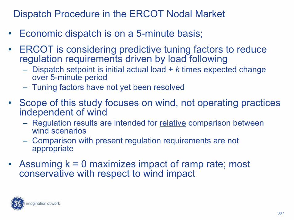
Dispatch Procedure in the ERCOT Nodal Market

• Economic dispatch is on a 5-minute basis; • ERCOT is considering predictive tuning factors to reduce

regulation requirements driven by load following– Dispatch setpoint is initial actual load + k times expected change

over 5-minute period– Tuning factors have not yet been resolved

• Scope of this study focuses on wind, not operating practices independent of wind– Regulation results are intended for relative comparison between

wind scenarios– Comparison with present regulation requirements are not

appropriate

• Assuming k = 0 maximizes impact of ramp rate; most conservative with respect to wind impact

81 /

Regulation Calculation in the Nodal Market

• Units on economicdispatch “step” to setpointsat discrete 5-minute points

• Difference between actual load and economic setpoints is defined as regulation– Positive deviations defined

as “Up Reg” (+REG)– Negative deviations

defined as “Down Reg” (-REG)

37,660

37,680

37,700

37,720

37,740

37,760

37,780

37,800

910 915 920 925 930

Minute

MW

LoadSetpoint

-100

-50

0

50

Regu

latio

n (M

W)

82 /

28,000

28,200

28,400

28,600

28,800

29,000

29,200

29,400

10 20 30 40 50 60

Minutes

MW

LoadSetpoints

-REG

-500

-400

-300

-200

-100

0

100

200

300

400

500

0 5 10 15 20 25Hours

MW

0

5,000

10,000

15,000

20,000

25,000

30,000

35,000

40,000

45,000

50,000

Inst. Regulation+REG-REGLoadDispatched Gen.

Regulation Through a Typical Day (without wind)

• Regulation is biased by load ramp rate – not just the“random jitter” component– Virtually no Down Reg during load rise– Virtually no Up Reg during load drop

83 /

Terminology and Abbreviations

The following terminology and abbreviations regarding regulation are used in this presentation:

Deployed Regulation – Maximum difference over each 5-minute period between the net load and the dispatch base point (actual net load at the beginning of period)

Procured Regulation – Amount of regulation “reserved” based on statistical analysis of prior deployments

+REG – Up Regulation – Positive difference between net load and base point.

-REG – Down Regulation - Difference between net load and base point (expressed in this presentation as a negative number)

84 /

Max. Hourly Deployed Regulation – January Example

• ~4 day time period plotted• Diurnal patterns visible

• ~4 days plotted• Diurnal pattern in REG are

visible• Significant impact of outliers

– A few driven by wind– Most outliers changed

incrementally– Some not changed at all

January

-800

-600

-400

-200

0

200

400

600

800

25 35 45 55 65 75 85 95 105 115 125

Hour

Max

. Hou

rly +

/-REG

Load Alone Load-5000Load-10000(1) Load-10000(2)Load-15000

0

200

400

600Peak caused by wind

Peak is ~same

85 /

Deployed Regulation Statistics

Up-Regulation

1124.9 MW1112.7 MW1105.6 MW1075.9 MW1072.5 MW

Maximum

23.1%12.7%14.2%6.4%

% Change

3.7%261.5 MW10.2%81.4 MW10,000 (2)4.9%285.8 MW16.5%86.1 MW15,000

3.1%265.2 MW11.7%82.5 MW10,000 (1)0.3%247.0 MW5.8%78.1 MW5,000

232.1 MW73.8 MW0

% Change

98th Percentile of 5-min Periods

% Change

Average Max of 5-min Periods

Wind (MW)

-566.4-565.9-554.9-538.9-522.2

Minimum

20.7%11.8%12.8%5.9%

% Change

8.4%-260.4 MW9.7%-81.5 MW10,000 (2)8.5%-281.2 MW16.5%-86.6 MW15,000

6.3%-262.7 MW11.7%-83.0 MW10,000 (1)3.2%-246.7 MW5.8%-78.6 MW5,000

-233.0 MW-74.3 MW0

% Change

98th Percentile of 5-min Periods

% Change

Average Min of 5-min Periods

Wind (MW)

Down-Regulation

86 /

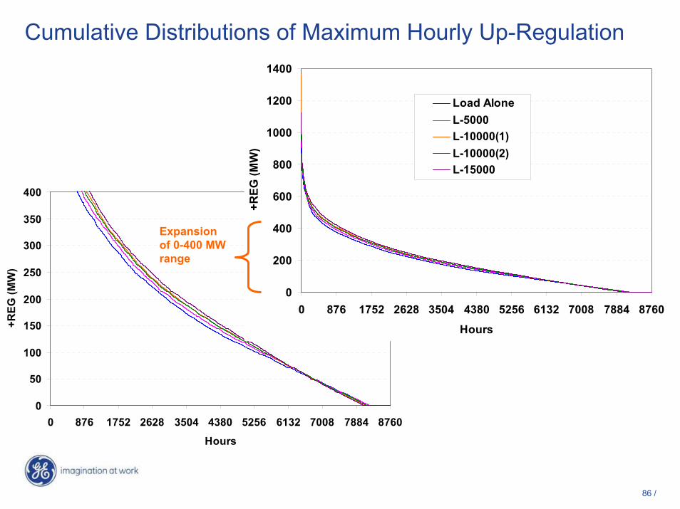
Cumulative Distributions of Maximum Hourly Up-Regulation

0

50

100

150

200

250

300

350

400

0 876 1752 2628 3504 4380 5256 6132 7008 7884 8760

Hours

+REG

(MW

)

Load AloneL-5000L-10000(1) L-10000(2) L-15000

Expansion of 0-400 MW range

0

200

400

600

800

1000

1200

1400

0 876 1752 2628 3504 4380 5256 6132 7008 7884 8760

Hours

+REG

(MW

)

Load AloneL-5000L-10000(1) L-10000(2) L-15000

87 /

-400

-350

-300

-250

-200

-150

-100

-50

0

0 876 1752 2628 3504 4380 5256 6132 7008 7884 8760

Hours -REG More Negative Than Value

-REG

(MW

)

Load AloneL-5000L-10000(1)L-10000(2) L-15000

Cumulative Distributions of Maximum Hourly Down-Regulation

Expansion of 0 - -400 MW range

-1400

-1200

-1000

-800

-600

-400

-200

0

0 876 1752 2628 3504 4380 5256 6132 7008 7884 8760

Hours

-REG

(MW

)

Load AloneL-5000L-10000(1)L-10000(2) L-15000

88 /

Extreme Up-Regulation and Down-Regulation

-1500

-1400

-1300

-1200

-1100

-1000

-900

-800

-700

-600

-500

0 20 40 60 80 100

Hours

-REG

(MW

)

Load AloneL-5000L-10000(1)L-10000(2) L-15000

600

700

800

900

1000

1100

1200

1300

1400

0 20 40 60 80 100

Hours

+REG

(MW

)

Load AloneL-5000L-10000(1) L-10000(2) L-15000

Except for an extreme outlier in one 10GW wind scenario, maximum, extreme +/-REG is increased modestly.

Increase ≈ proportionate with the amount of wind resources

≈ 100 MW increase

100 hrs is ≈ 1.2% of year

89 /

Hourly Maximum Regulation Increase with 15,000 MW Wind

0%

5%

10%

15%

20%

25%

−280 → −300

−260 → −280

−240 → −260

−220 → −240

−200 → 220

−180 → −200

−160 → −180

−140 → −160

−120 → −140

−100 → −120

−80 → −100

−60 → −80

−40 → −60

−20 → −40

0 → −20

0 → 20

20 → 40

40 → 60

60 → 80

80 → 100

100 → 120

120 → 140

140 → 160

160 → 180

180 → 200

200 → 220

220 → 240

240 → 260

260 → 280

280 → 300

Change in Regulation

Perc

ent o

f Hou

rs+REG-REG

Difference between hourly max. regulation for load only and load –15GW wind

-18.217.7Mean

-287.2

444.2

64.9

+REG

265.3Maximum

Minimum

Sigma

-453.1

65.1

-REG

Results are ≈ symmetric

These statistics describe the maximum regulation within each 1-hr period

90 /

Up Regulation Correlation with Time of Day and Month98.8th Percentile of +REG Deployed

1 3 5 7 9 11 13 15 17 19 21 23

Jan

Mar

May

Jul

Sep

Nov

600-800400-600200-4000-200

Load Alone

1 3 5 7 9 11 13 15 17 19 21 23

Jan

Mar

May

Jul

Sep

Nov

800-1000600-800400-600200-4000-200

Load – 5000 MW Wind

Load – 10,000 MW Wind (1) Load – 15,000 MW Wind

1 3 5 7 9 11 13 15 17 19 21 23

Jan

Mar

May

Jul

Sep

Nov

800-1000600-800400-600200-4000-200

1 3 5 7 9 11 13 15 17 19 21 23

Jan

Mar

May

Jul

Sep

Nov

800-1000600-800400-600200-4000-200

91 /

Differential Up Regulation Requirements for 15 GW Wind1 3 5 7 9 11 13 15 17 19 21 23

Jan

Mar

May

Jul

Sep

Nov 250-300200-250150-200100-15050-1000-50-50-0-100--50

98.8th Percentile of +REG Deployed

• Increases during morning load ramp due to wind decline• Increases during early evening during spring and fall

92 /

Differential Down Regulation Requirements for 15 GW Wind98.8th Percentile of –REG Deployed

1 3 5 7 9 11 13 15 17 19 21 23

Jan

Mar

May

Jul

Sep

Nov 50-1000-50-50-0-100--50-150--100-200--150-250--200-300--250

• More down regulation in the evening, particularly in fall, winter and spring

• Decreased down regulation during summer mornings

93 /

Variation in Up Regulation for Selected Periods

0

100

200

300

400

500

600

0 5000 10000 15000Wind Capacity (MW)

+REG

(a

vera

ge m

onth

ly 9

8.8th

per

cent

ile)

Morning (0700 - 1000)Evening (1800)Mid-Day (1400)Night (2300)

+16.3%

+52.0%

+65.2%

+25.6%

• Relative impact is not uniform, wind does substantially increaseregulation requirements at times when regulation requirements had been small to moderate

• Linearity allows scale-up of regulation procurement to accommodate year-to-year wind additions

94 /

Increase of Evening Down Regulation Requirements

-600

-500

-400

-300

-200

-100

0

0 5000 10000 15000

Wind Capacity (MW)

-REG

(a

vera

ge m

onth

ly 9

8th

perc

entil

e)

31.9%

Evening wind increase coincides with load drop

95 /

Impact of Wind Penetration on Regulation

• Regulation peaks caused by load ramping are incrementally increased due to added ramp caused by wind

• Relative to load alone, 98th percentile of regulation increases on the order of 20% - 23% at 15 GW of wind

• Regulation increases linearly with wind penetration

• Extrema appear both with and without wind, with magnitudes incrementally greater with 15 GW of wind

• Largest changes are concentrated in particular times of day and seasons -- +REG in the evenings increases 65%

96 /

Evaluation of RegulationProcurement Methodology

97 /

In this next set of slides, we will show:• How ERCOT presently determines the amount of

regulation to procure• The robustness of this methodology to increased

wind penetrationKey issues are:• Frequency of under-procurement• Severity of under-procurement

98 /

ERCOT Regulation Procurement Methodology

0

100

200

300

400

500

600

700

800

25 35 45 55 65 75

Hour

Max

. Hou

rly +

REG

Deployed +REG, Load AloneProcured +REG, Load Alone

Deployed > Procured

• Regulation procurement algorithm seeks to cover most, but not all time periods; occasional “misses” are expected

• Procurement based on 98.8th percentile of maximum deployment in 5-minute intervals for same hour of day in:– Same month, prior year– Prior month, same year

99 /

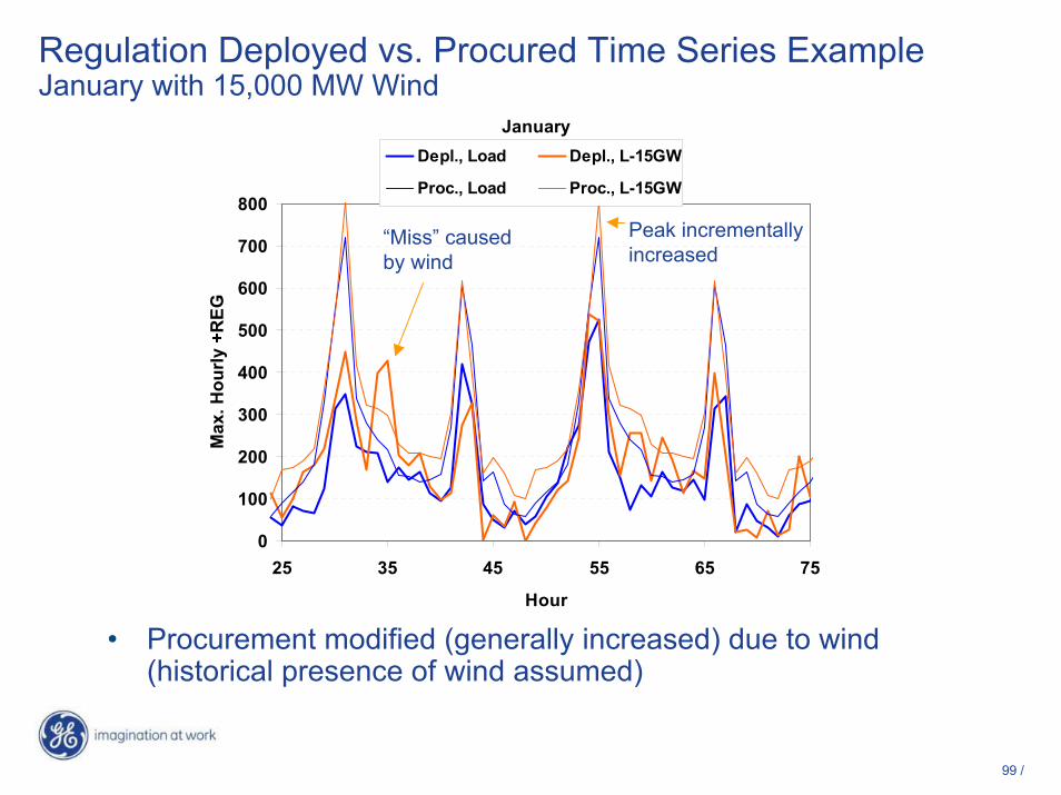
Regulation Deployed vs. Procured Time Series Example January with 15,000 MW Wind

January

0

100

200

300

400

500

600

700

800

25 35 45 55 65 75

Hour

Max

. Hou

rly +

REG

Depl., Load Depl., L-15GW

Proc., Load Proc., L-15GW

• Procurement modified (generally increased) due to wind (historical presence of wind assumed)

“Miss” caused by wind

Peak incrementally increased

100 /

Changes in Deployed and Procured Regulation

0

200

400

600

800

1000

1200

0 5000 10000 15000

Wind Capacity (MW)

Up

Reg

ulat

ion

(MW

)

Max Deployed98.8 pct DeployedMean DeployedMean ProcuredMax. Procured

+4.9%

+23.1%

+16.5%-800

-700

-600

-500

-400

-300

-200

-100

0

0 5000 10000 15000

Wind Capacity (MW)

Dow

n R

egul

atio

n (M

W)

Min Deployed98.8 pct DeployedMean DeployedMean ProcuredMin. Procured

16.5%

20.7%

8.5%

• Gap between maximum deployed and maximum procured narrows as wind penetration increases

• Point of comparison: sigma of 5-min delta increased 18% from load alone to load minus 15 GW of wind

101 /

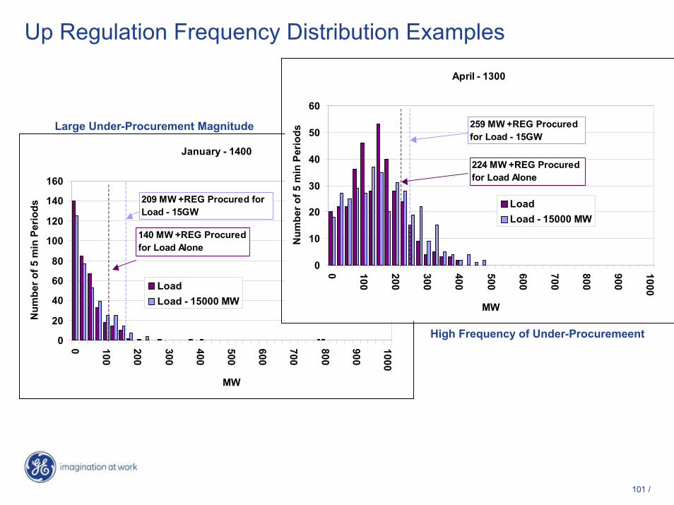
Up Regulation Frequency Distribution Examples

January - 1400

0

20

40

60

80

100

120

140

160

0 100

200

300

400

500

600

700

800

900

1000

MW

Num

ber o

f 5 m

in P

erio

ds

LoadLoad - 15000 MW

209 MW +REG Procured for Load - 15GW

140 MW +REG Procured for Load Alone

April - 1300

0

10

20

30

40

50

60

0 100

200

300

400

500

600

700

800

900

1000

MWN

umbe

r of 5

min

Per

iods

LoadLoad - 15000 MW

259 MW +REG Procured for Load - 15GW

224 MW +REG Procured for Load Alone

Large Under-Procurement Magnitude

High Frequency of Under-Procuremeent

102 /

Percentage of Hours with +REG Under-Procurement

1 3 5 7 9 11 13 15 17 19 21 23

Jan

Mar

May

Jul

Sep

Nov5.0%-6.0%4.0%-5.0%3.0%-4.0%2.0%-3.0%1.0%-2.0%0.0%-1.0%

Load Alone

Load – 15,000 MW Wind

1 3 5 7 9 11 13 15 17 19 21 23

Jan

Mar

May

Jul

Sep

Nov5.0%-6.0%4.0%-5.0%3.0%-4.0%2.0%-3.0%1.0%-2.0%0.0%-1.0%

14.7% peak

11.7% peak

Present approach has a relatively large number of misses in the spring (morning to mid-afternoon) and autumn evenings

Increased overall +REG deployment with 15 GW of wind diminishes the high concentration of misses during these periods

A few limited points were somewhat more severe

10.3% peak

103 /

Root Mean Square of +REG Under-ProcurementLoad Alone Load – 15,000 MW Wind

1 3 5 7 9 11 13 15 17 19 21 23

Jan

Mar

May

Jul

Sep

Nov

300-400200-300100-2000-100

0000

1 3 5 7 9 11 13 15 17 19 21 23

Jan

Mar

May

Jul

Sep

Nov

400-50300-40200-30100-200-100

1 3 5 7 9 11 13 15 17 19 21 23

Jan

Mar

May

Jul

Sep

Nov

0-100

-100-0

-200--100

Difference

104 /

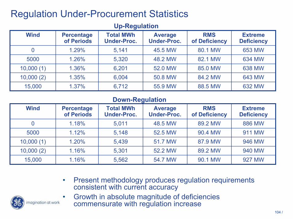
Regulation Under-Procurement Statistics

• Present methodology produces regulation requirements consistent with current accuracy

• Growth in absolute magnitude of deficiencies commensurate with regulation increase

88.5 MW84.2 MW85.0 MW82.1 MW80.1 MW

RMSof Deficiency

643 MW50.8 MW6,0041.35%10,000 (2)632 MW55.9 MW6,7121.37%15,000

638 MW52.0 MW6,2011.36%10,000 (1)634 MW48.2 MW5,3201.26%5000653 MW45.5 MW5,1411.29%0

ExtremeDeficiency

AverageUnder-Proc.

Total MWhUnder-Proc.

Percentage of Periods

WindUp-Regulation

90.1 MW89.2 MW87.9 MW90.4 MW89.2 MW

RMSof Deficiency

940 MW52.2 MW5,3011.16%10,000 (2)927 MW54.7 MW5,5621.16%15,000

946 MW51.7 MW5,4391.20%10,000 (1)911 MW52.5 MW5,1481.12%5000886 MW48.5 MW5,0111.18%0

ExtremeDeficiency

AverageUnder-Proc.

Total MWhUnder-Proc.

Percentage of Periods

WindDown-Regulation

105 /

In summary:• Regulation requirements for net load with high wind

penetration are statistically as “well behaved” as load only• The present ERCOT methodology for determining the

amount of regulation to procure remains effective with 15 GW of wind

• Linearity allows scale-up of regulation procurement to accommodate year-to-year wind additions

• Under-procurements are not substantially more severe• There may be improvements which might be made to the

methodology to reduce the amount of regulation procured while maintaining accuracy of procurement

106 /

Production Simulation

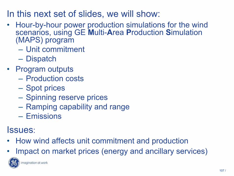
107 /

In this next set of slides, we will show:• Hour-by-hour power production simulations for the wind

scenarios, using GE Multi-Area Production Simulation (MAPS) program– Unit commitment– Dispatch

• Program outputs– Production costs– Spot prices– Spinning reserve prices– Ramping capability and range– Emissions

Issues:• How wind affects unit commitment and production• Impact on market prices (energy and ancillary services)

108 /

Energy Output Commitment Based on State-of-Art Forecast

0

20,000

40,000

60,000

80,000

100,000

120,000

140,000

160,000

CC GT STCOAL STNG WIND

Ener

gy (G

Wh)

Zero Wind5 GW Wind10 GW Wind - Case 110 GW Wind - Case 215 GW Wind

Major impact is on combined cycle unit operation, consistent with results observed in other studies

109 /

Peak Load Week (Aug 11-18) - State of the Art Forecast

0

10000

20000

30000

40000

50000

60000

70000

80000

1 8 15 22 29 36 43 50 57 64 71 78 85 92 99 106 113 120 127 134 141 148 155 162

Hour

MW

HYDRO NUCLEAR STEAM COAL WIND COMB. CYCLE STEAM GAS GAS TURBINE

0

10000

20000

30000

40000

50000

60000

70000

1 8 15 22 29 36 43 50 57 64 71 78 85 92 99 106

113

120

127

134

141

148

155

162

Hour

MW


Zero Wind - DispatchZero Wind - Commitment

15 GW Wind - Commitment 15 GW Wind - Dispatch

0

10000

20000

30000

40000

50000

60000

70000

80000

1 8 15 22 29 36 43 50 57 64 71 78 85 92 99 106 113 120 127 134 141 148 155 162

Hour

MW

0

10000

20000

30000

40000

50000

60000

70000

80000

1 8 15 22 29 36 43 50 57 64 71 78 85 92 99 106 113 120 127 134 141 148 155 162

Hour

MW


110 /

0

5000

10000

15000

20000

25000

30000

35000

40000

45000

1 8 15 22 29 36 43 50 57 64 71 78 85 92 99 106 113 120 127 134 141 148 155 162

Hour

MW

NUCLEAR HYDRO STEAM COAL WIND COMB. CYCLE STEAM GAS GAS TURBINE

0

5000

10000

15000

20000

25000

30000

35000

40000

45000

50000

1 8 15 22 29 36 43 50 57 64 71 78 85 92 99 106 113 120 127 134 141 148 155 162

Hour

MW


Zero Wind - DispatchZero Wind - Commitment

15 GW Wind - Dispatch

05000

100001500020000250003000035000400004500050000

1 8 15 22 29 36 43 50 57 64 71 78 85 92 99 106 113 120 127 134 141 148 155 162

Hour

MW

05000

100001500020000250003000035000400004500050000

1 8 15 22 29 36 43 50 57 64 71 78 85 92 99 106 113 120 127 134 141 148 155 162

Hour

MW

Peak Wind Week (April 2-9) - State of the Art Forecast

15 GW Wind - Commitment


111 /

Production Cost Reductions Due to Wind

0.00

10.00

20.00

30.00

40.00

50.00

60.00

5 GW Wind 10 GW Wind - Case 1 10 GW Wind - Case 2 15 GW Wind

Cos

t Sav

ings

($/M

Wh)

Value of wind decreases slightly with increased wind penetration

112 /

Total Annual Emissions (State-of-Art Wind Forecast Assumed)

54,000

56,000

58,000

60,000

62,000

64,000

66,000

68,000

Zero Wind 5 GW Wind 10 GWWind -Case 1

10 GWWind -Case 2

15 GWWind

NOx (TONS)

160,000,000165,000,000170,000,000175,000,000180,000,000185,000,000190,000,000195,000,000200,000,000205,000,000

Zero Wind 5 GWWind

10 GWWind -Case 1

10 GWWind -Case 2

15 GWWind

CO2 (TONS)

590,000

600,000

610,000

620,000

630,000

640,000

650,000

660,000

Zero Wind 5 GW Wind 10 GWWind -Case 1

10 GWWind -Case 2

15 GWWind

SO2 (TONS)

113 /

Energy Spot Prices – Assumes State of the Art Forecast

0

20

40

60

80

100

120

140

160

180

0 1000 2000 3000 4000 5000 6000 7000 8000 9000

Hours

Spot

Pric

e($/

MW

h)

No Wind5 GW10 GW - Case 110 GW - Case 215 GW

114 /

Impact of Wind Forecast on Energy Prices – 15 GW Wind

0

20

40

60

80

100

120

140

160

180

0 1000 2000 3000 4000 5000 6000 7000 8000

Hour

Spot

Pric

e ($

/MW

h)

Zero WindNo ForecastStudy Year ForecastPerfect Forecast

Good forecasts minimize reductions in spot prices and reduce overall energy cost; due to less over-commitment

S-o-A Forecast

115 /

In summary:

• Emissions and nodal energy prices decrease as wind penetration increases

• Value of wind per MWh decreases slightly with increased wind penetration

• Bulk of energy displacement is from combined cycle units

• Lack of wind forecast results in significant over commitment of units – depressing nodal prices

116 /

Available Regulation Range

117 /

In this next set of slides, we will show:• How the changes in unit commitment and dispatch

affect the ability to meet regulation requirements with increased wind penetration

Key issues are:• Displacement of conventional generation• Flexibility of committed units

118 /

Down Regulation Resources Based on state of the art forecast

0

200

400

600

800

1000

1200

1400

1600

1 8 15 22 29 36 43 50 57 64 71 78 85 92 99 106 113 120 127 134 141 148 155 162Hour

MW

/Min

GAS TURBINE

STEAM GAS

COMB. CYCLE

STEAM COAL

HYDRO

0

500

1000

1500

2000

2500

3000

1 8 15 22 29 36 43 50 57 64 71 78 85 92 99 106 113 120 127 134 141 148 155 162Hour

MW

/Min

Gas TurbineSteam GasCombined CycleSteam CoalHydro

Zero Wind

0

500

1000

1500

2000

2500

3000

1 8 15 22 29 36 43 50 57 64 71 78 85 92 99 106 113 120 127 134 141 148 155 162Hour

MW

/Min

Gas TurbineSteam GasCombined CycleSteam CoalHydro

15 GW Wind

0

200

400

600

800

1000

1200

1400

1600

1800

1 8 15 22 29 36 43 50 57 64 71 78 85 92 99 106 113 120 127 134 141 148 155 162Hour

MW

/Min

GAS TURBINESTEAM GASCOMB. CYCLESTEAM COALHYDROZero Wind 15 GW Wind

Min Load Week (March 20-27)

Peak Load Week (August 11-18)

Hydro Steam Coal Combined Cycle Steam Gas Gas Turbine

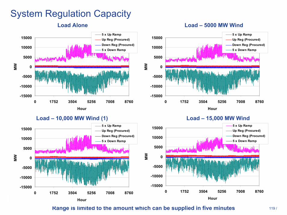
119 /

System Regulation CapacityLoad Alone Load – 5000 MW Wind

Load – 10,000 MW Wind (1) Load – 15,000 MW Wind

Range is limited to the amount which can be supplied in five minutes

-15000

-10000

-5000

0

5000

10000

15000

0 1752 3504 5256 7008 8760

Hour

MW

5 x Up RampUp Reg (Procured)Down Reg (Procured)5 x Down Ramp

-15000

-10000

-5000

0

5000

10000

15000

0 1752 3504 5256 7008 8760

Hour

MW


-15000

-10000

-5000

0

5000

10000

15000

0 1752 3504 5256 7008 8760

Hour

MW


-15000

-10000

-5000

0

5000

10000

15000

0 1752 3504 5256 7008 8760

Hour

MW


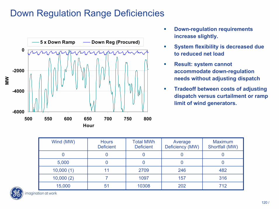
120 /

Down Regulation Range DeficienciesDown-regulation requirements increase slightly.

System flexibility is decreased due to reduced net load

Result: system cannot accommodate down-regulation needs without adjusting dispatch

Tradeoff between costs of adjusting dispatch versus curtailment or ramp limit of wind generators.

-6000

-4000

-2000

0

500 550 600 650 700 750 800Hour

MW

5 x Down Ramp Down Reg (Procured)

3161571097710,000 (2)

712202103085115,000

48224627091110,000 (1)

00005,000

00000

MaximumShortfall (MW)

AverageDeficiency (MW)

Total MWhDeficient

HoursDeficient

Wind (MW)

121 /

Regulation Range

• Up-regulation range margin is reduced, but remains ample– Assuming 5-minute delivery– Margin could be less if a faster delivery is required

• Down-regulation range becomes an occasional issue for > 5,000 MW of wind– Committed conventional units are pushed toward their minimum

load levels– Relatively few hours are involved for wind levels investigated

• Alternatives– Conventional units can be de-committed to provide range,

can adversely impact economics during the next day– Allow wind plants to provide down-regulation– Apply up-ramp limits on wind generation– Curtail wind output

• Future operations will require increased flexibility from balance of generation

122 /

Regulation ServiceCosts

123 /

In this next set of slides, we will show:• The impact of wind on per-unit costs of regulation

services• The costs of increased regulation services to

accommodate wind penetration• Emphasis on relative metrics

124 /

0

10

20

30

40

50

60

70

80

90

100

0 1000 2000 3000 4000 5000 6000 7000 8000Hours

Cos

t of S

pin

($/M

Wh)


State of Art Forecast

0

10

20

30

40

50

60

70

80

90

100

0 1000 2000 3000 4000 5000 6000 7000 8000Hours

Cos

t of S

pin

($/M

Wh)


No Forecast

0

10

20

30

40

50

60

70

80

90

100

0 1000 2000 3000 4000 5000 6000 7000 8000Hours

Cos

t of S

pin

($/M

Wh)


Perfect Forecast

Spin Cost for Various Wind Penetrations

125 /

Regulation Cost Assumptions

• REG cost is the greater of $5/MWh or the cost of spinning reserve

• Cost of wind curtailment added when –REG exceeds available range (spot price)

• Results most useful when considered on a relative basis

126 /

Cost of Meeting Regulation Service Requirements – S-o-A Forecast

• Reduction of net load slightly decreases per MWh cost of +REG and –REG, up through 10,000 MW scenarios

• Excess unit commitments due to load forecast errors, and reduced net load sharply drops regulation cost at 15,000 MW

0

2,000,000

4,000,000

6,000,000

0 5000 10000 15000Wind Capacity (MW)

Proc

ured

REG

MW

h

Total+REG-REG

75%

80%

85%

90%

95%

100%

105%

None 50

0010

,000 (

1)10

,000 (

2)15

,000

Wind Capacity (MW)

Rel

ativ

e C

ost o

f REG

pe

r MW

h Pr

ocur

ed

+REG-REG

0%

20%

40%

60%

80%

100%

120%

None 5000 10,000(1)

10,000(2)

15,000

Wind Scenario

Rel

ativ

e C

ost o

f Pro

cure

d R

EG

Total+REG-REG

127 /

Cost of Meeting Regulation Service Requirements –Perfect Forecast

• Reduced unit over-commitment allows unit costs of regulation to decrease gradually as net load is reduced by increased wind

• Total cost of +/- REG increases at a much lower rate than linear with respect to wind capacity

0

2,000,000

4,000,000

6,000,000

0 5000 10000 15000Wind Capacity (MW)

Proc

ured

REG

MW

h

Total+REG-REG

75%

80%

85%

90%

95%

100%

105%

None 50

0010

,000 (

1)10

,000 (

2)15

,000

Wind Capacity (MW)

Rel

ativ

e C

ost o

f REG

pe

r MW

h Pr

ocur

ed

+REG-REG

0%

20%

40%

60%

80%

100%

120%

None 5000 10,000(1)

10,000(2)

15,000

Wind Scenario

Rel

ativ

e C

ost o

f Pro

cure

d R

EG

Total+REG-REG

128 /

Regulation Costs Summary

• Per-unit costs of regulation are highly dependent on impacts of wind on dispatch

• Imperfect wind forecast leads to unit excess unit commitment, reducing regulation costs

• Results are volatile, makeup of future generation portfolio is critical

$0.07636,180,453$143.05$72.49$69.3610,000 (2)

$0.10737,037,236$142.30$72.93$70.1210,000 (1)

-$0.18053,933,379$129.37$67.94$61.4415,000

$0.17917,940,311$139.09$72.76$69.545,000

$0.14453,933,379$141.85$74.83$72.0115,000

$0.20036,180,453$146.33$76.21$70.1210,000 (2)

$0.27737,037,236$149.35$78.14$71.2210,000 (1)

$0.11217,940,311$141.11$73.21$67.905,000

0$139.09$72.21$66.880

Inc. Cost of Regulation

($/MWh)

Total Wind Generation

(MWh)

Total Reg. Cost

($MM)

Reg-DownCost

($MM)

Reg-Up Cost

($MM)

Wind Capacity

(MW)

State-of-Art Wind Forecast

Perfect Wind

Forecast

-$0.30

-$0.20

-$0.10

$0.00

$0.10

$0.20

$0.30

5000 10,000 (1) 10,000 (2) 15,000

Wind Scenario (MW)

Incr

emen

tal C

ost o

f REG

($/M

Wh)

(MW

h of

Tot

al W

ind

Prod

uctio

n)

S-o-A ForecastPerfect Forecast

129 /

Forecast Error AnalysisImpact on Non-Spinning Reserves

130 /

Predictability Analysis

131 /

Day-ahead predictability of net load is important to unit commitment; inaccuracies increase operating costs and may require greater A/S procurement.The next slides analyze net load predictability

132 /

Time of Year Predictability Analysis

133 /

Load Yearly Average Profile and Largest Forecast ErrorsStudy Year Load with 15000 MW of Wind

-18000

-12000

-6000

0

6000

12000

18000

24000

30000

36000

42000

48000

54000

Act

ual a

nd D

ay-A

head

Loa

d (M

W)

-9000

-6000

-3000

0

3000

6000

9000

12000

15000

18000

21000

24000

27000

Max

/Min

For

ecas

t Err

or (M

W)

Load ActualLoad ForecastMax Pos Forecast ErrorMax Neg Forecast Error


Winter

Spring

Summer

Fall

May 20th: Largest Neg Load Forecast Error

Aug 28th: Largest Pos Load Forecast ErrorMarch 27th

Min Load Day

August 17th

Peak Load Day

Max L-W Error = 10294 MW (Aug 28th)MAE = 1296 MW (3.5% of Average)RMSE = 1792 MW (4.9% of Average)Sigma = 1755 (4.8% of Average)

Greater tendency to over-forecast load during the summer months

134 /

Net Load Yearly Average Profile and Largest Forecast ErrorsStudy Year Load with 15000 MW of Wind

-18000

-12000

-6000

0

6000

12000

18000

24000

30000

36000

42000

48000

54000

Act

ual a

nd D

ay-A

head

Loa

d-W

ind

(MW

)

-9000

-6000

-3000

0

3000

6000

9000

12000

15000

18000

21000

24000

27000

Max

/Min

For

ecas

t Err

or (M

W)

Load-Wind ActualLoad-Wind ForecastMax Pos Forecast ErrorMax Neg Forecast Error


Winter

Spring

Summer

Fall

Mar 11th: Largest Neg L-W Forecast Error

Aug 28th: Largest Pos L-W Forecast Error

March 27th

Min Net Load Day

July 17th Peak Net Load Day

Max L-W Error = 9675 MW (Aug 28th)MAE = 1698 MW (5.5% of Average)RMSE = 2199 MW (7.2% of Average)Sigma = 2149 (7.0% of Average)

Wind generally increases net-load forecast errors in Winter and Spring more than Summer

135 /

Net Load and Wind Day-Ahead Predictability – Summary (Study Year Data)

5,000 MW 10,000 MW 15,000 MW

0

300

600

900

1200

1500

1800

Erro

r (M

W)

20

30

40

50

60

70

80

% E

rror

MAE (MW)RMSE (MW)%MAE%RMSE

2149(7.0)

1887(5.8)

1928(5.9)

1762(5.1)

1755 (4.8)

Std DevMW(%)

1698(5.5)

1467(4.5)

1505(4.6)

1338(3.8)

1296(3.5)

MAE*MW(%)

9765

9786

9763

9951

10294

Max Error (MW)

1936(5.9)

Load w/ 10,000 MW Wind (2)

1792(4.9)

Base Case: Load w/ no Wind

1805(5.2)

Load w/ 5000 MW Wind

2199(7.2)

1974(6.0)

RMSE**MW(%)

Load w/ 15,000 MW Wind

Load w/ 10,000 MW Wind (1)

Case

* Mean absolute error ** Root mean square error – more affected by large deviations

-59211614(26.3)

1294(21.1)

1611(26.2)

15,000 MW Wind

-40781096(26.6)

876(21.3)

1093(26.5)

10,000 MW Wind (2)

-42641169(27.7)

935(22.2)

1167(27.7)

10,000 MW Wind (1)

-2529639(31.3)

511(25.0)

638(31.2)

5000 MW Wind

Error = forecast – actual

500

1000

1500

2000

2500

Erro

r (M

W)

3%

6%

9%

12%

15%

% E

rror

MAE (MW)RMSE (MW)%MAE%RMSE

Load L-5,000 MW L-10,000 MW L-15,000 MW

Wind absolute error (MW) increases slower than average output

Absolute error (MW) and percent error increase linearly

Net Load

Wind

NB: Percent errors based on average output

136 /

Hourly Wind Predictability (Forecast Errors*) (Study Year Data)

0

200

400

600

800

1000

1200

1400

1600

1800

< -4500-4500 – -4200-4200 – -3900-3900 – -3600-3600 – -3300-3300 – -3000-3000 – -2700-2700 – -2400-2400 – -2100-2100 – -1800-1800 – -1500-1500 – -1200-1200 – -900-900 – -600-600 – -300-300 – 00 – 300300 – 600600 – 900900 – 12001200 – 15001500 – 18001800 – 21002100 – 24002400 – 27002700 – 30003000 – 33003300 – 36003600 – 39003900 – 42004200 – 4500> 4500

MW

Hou

rs

5000 MW Wind10000 MW Wind (1)10000 MW Wind (2)15000 MW Wind

Wind forecast error increases with wind, skewed to the left … tendency to under-forecast wind

Extreme Forecast Errors* Error = forecast – actual

Over-Commitment

Under-Commitment

910 / 364296 / 19384 / 418 / 0> ± 2300 MW (−/+)

67 / 00 / 00 / 00 / 0> ± 4600 MW (−/+)

43 / 048 / 038 / 033 / 0>µ ± 3σ (−/+)

121 / 1

10,000 MW Wind (2)

125 / 2

10,000 MW Wind (1)

114 / 1107 / 9>µ ± 2.5σ (−/+)

5000 MW Wind

15,000 MW Wind

137 /

0

100

200

300

400

500

600

700

800

900

1000

1100

1200

< -6000-6000 – -5600-5600 – -5200-5200 – -4800-4800 – -4400-4400 – -4000-4000 – -3600-3600 – -3200-3200 – -2800-2800 – -2400-2400 – -2000-2000 – -1600-1600 – -1200-1200 – -800-800 – -400-400 – 00 – 400400 – 800800 – 12001200 – 16001600 – 20002000 – 24002400 – 28002800 – 32003200 – 36003600 – 40004000 – 44004400 – 48004800 – 52005200 – 56005600 – 6000> 6000

MW

Hou

rs

Load-aloneLoad-5000 MWLoad-15000 MW

Hourly Load-Wind Predictability (Forecast Errors*) (Study Year Data)

Wind adds to overall net load forecast error and increases number of extreme deviations … tendency to over-forecast net load

* Error = forecast – actual

Under-Commitment

Over Commitment

731 / 1591547 / 1357413 / 1048> ± 2300 MW (−/+)

51 / 217

17 / 74

67 / 152

W/ 5000 MW Windσ = 1762 Using load σ

17 / 77

66 / 160

51 / 12910 / 4315 / 95>µ ± 3σ (−/+)

132 / 27151 / 11164 / 185>µ ± 2.5σ (−/+)

26 / 186

Load-alone σ = 1755

> ± 4600 MW (−/+) 72 / 316

W/ 15000 MW Windσ = 2149 Using load σ

Extreme Forecast Errors

138 /

-6000

-4000

-2000

0

2000

4000

6000

-8000 -4000 0 4000 8000 12000

Load Forecast Error

Win

d Fo

reca

st E

rror

WinterSpringSummerFall

Correlation of Load and Wind Forecast Errors By Season (Study Year Load and 15000 MW of Wind)

10294 MW-6291 MW

R2 = .034

Over-commitment

Under-commitment

Under-commitment

Over-commitment

Increase L-W over-forecast

Increase L-W under-forecast Load and Wind

errors offset

Load and Wind errors offset

Q1Q2

Q3

Q4Q3

139 /

Correlation of Load and Wind Forecast Errors By Season (Study Year Load W/ 15000 MW)

-6000

-4000

-2000

0

2000

4000

6000

-8000 -4000 0 4000 8000 12000

Load Error

Win

d Er

ror

Winter

-6000

-4000

-2000

0

2000

4000

6000

-8000 -4000 0 4000 8000 12000

Load Error

Win

d Er

ror

Spring

-6000

-4000

-2000

0

2000

4000

6000

-8000 -4000 0 4000 8000 12000

Load Error

Win

d Er

ror

Summer

-6000

-4000

-2000

0

2000

4000

6000

-8000 -4000 0 4000 8000 12000

Load Error

Win

d Er

ror

Fall

Over-commitment

Under-commitment

Under-commitment

Over-commitment

Increase L-W Over-forecast

Increase L-W Under-forecast



Risk of simultaneousunder-commitment error is very small

Q1Q2

Q3 Q4

140 /


Hour of Day

Mon

th o

f Yea

r

-2000-0-4000--2000-6000--4000-8000--6000

Timing of Negative Load Forecast Errors (Under-Commitment) (Study Year)

Largest load under-forecasts typically occur in the afternoon and early evening during Winter and early Spring

-6291 MW

-6272 MW

141 /

Timing of Negative Net-Load (Under-Commitment) Forecast Errors(Study Year Load with 15000 MW of Wind)


Hour of Day -2000-0-4000--2000-6000--4000-8000--6000

Large net-load under-forecasts much more spread with over the year due to spread in wind forecast errors. Extreme errors tend to occur in Winter and early Spring.

-7781 MW

-7322 MW

-6099 MW

-6083 MW

Mon

th o

f Yea

r

142 /

Incremental Under-Forecast Errors Due to Wind (Study Year Load with 15000 MW of Wind)


Hour of Day

Mon

th o

f Yea

r

1000-2500-500-1000-2000--500-3500--2000

15000 MW of wind tends to cause a moderately widespread increase in forecast uncertainty

-3028 MW

-2965 MW

-2605 MW

-2229 MW

-2338 MW

-2463 MW

-2631 MW

143 /

January Hourly Load and Net Load Forecast Errors (Study Year Load with 15000 MW of Wind)


Hour of Day

Fore

cast

Err

ors

(MW

)

Tota

l Loa

d (M

W)

0 1 2 3 4 5 6 7 8 9 10 11 12 13 14 15 16 17 18 19 20 21 22 23 24 250

4500

9000

13500

18000

22500

27000

31500

36000

-8000

-6000

-4000

-2000

0

2000

4000

6000

8000

-8000

-6000

-4000

-2000

0

2000

4000

6000

8000

Load ErrorsLoad-Wind ErrorsTotal LoadLoad-Wind

Risk that wind curtailmentcould be infrequently needed

Tends to be available resources

144 /

July Hourly Load and Net Load Forecast Errors (Study Year Load with 15000 MW of Wind)


Hour of Day

Fore

cast

Err

ors

(MW

)

Tota

l Loa

d (M

W)

-8000

-6000

-4000

-2000

0

2000

4000

6000

8000

0 1 2 3 4 5 6 7 8 9 10 11 12 13 14 15 16 17 18 19 20 21 22 23 24 250

7500

15000

22500

30000

37500

45000

52500

60000

-8000

-6000

-4000

-2000

0

2000

4000

6000

8000

Load ErrorsLoad-Wind ErrorsTotal LoadLoad-Wind

145 /

Observations and Conclusions

• Risk of under-commitment tends to occur off-peak when impact is low– Under-commitment aggravated by using a higher

confidence level wind forecast• During summer peak hours, wind forecast error tends to

partially cancel apparent bias in mean load forecast towards over-commitment

• Increased wind penetration does not create an obvious requirement for across-the-board non-spin reserve requirements increase– Periods where uncertainty is high and resources are tight

may require addition of NSRS– Consider a longer-term NSRS service

146 /

• Addition of wind requires a moderate increase of ancillary service requirements

• At certain low-load, high-wind conditions, providing down-regulation can be a challenge

• Present ERCOT procurement methodologies:– Regulation algorithm adequate, some incremental improvements are

possible– Responsive reserve procedure adequate, may need to account

for predicted wind risk periods– Non-spin can be a preferable alternative to carrying large amounts

of RRS during high-risk periods• Increased regulation services create a small increment (1%) in cost

relative to value of MWh supplied by wind

Overall Conclusions

Comments of CLECA on RETI Draft Phase 1A Report of CLECA on RETI Draft Phase 1A Report ......

Documents

Transcript of Comments of CLECA on RETI Draft Phase 1A Report of CLECA on RETI Draft Phase 1A Report ......