Combustion Science and Technology Application of ...

PLEASE SCROLL DOWN FOR ARTICLE

This article was downloaded by: [University of Southern California]On: 11 January 2011Access details: Access Details: [subscription number 911085157]Publisher Taylor & FrancisInforma Ltd Registered in England and Wales Registered Number: 1072954 Registered office: Mortimer House, 37-41 Mortimer Street, London W1T 3JH, UK

Combustion Science and TechnologyPublication details, including instructions for authors and subscription information:http://www.informaworld.com/smpp/title~content=t713456315

Application of Continuation Methods to Plane Premixed Laminar FlamesV. Giovangiglia; M. D. Smookeb

a Centre de Mathématiques Appliquées and CNRS. Ecole Polytechnique, Palaiseau cedex, France b

Department of Mechanical Engineering, Yale University, New Haven, CT, USA

To cite this Article Giovangigli, V. and Smooke, M. D.(1993) 'Application of Continuation Methods to Plane PremixedLaminar Flames', Combustion Science and Technology, 87: 1, 241 — 256To link to this Article: DOI: 10.1080/00102209208947217URL: http://dx.doi.org/10.1080/00102209208947217

Full terms and conditions of use: http://www.informaworld.com/terms-and-conditions-of-access.pdf

This article may be used for research, teaching and private study purposes. Any substantial orsystematic reproduction, re-distribution, re-selling, loan or sub-licensing, systematic supply ordistribution in any form to anyone is expressly forbidden.

The publisher does not give any warranty express or implied or make any representation that the contentswill be complete or accurate or up to date. The accuracy of any instructions, formulae and drug dosesshould be independently verified with primary sources. The publisher shall not be liable for any loss,actions, claims, proceedings, demand or costs or damages whatsoever or howsoever caused arising directlyor indirectly in connection with or arising out of the use of this material.

http://www.informaworld.com/smpp/title~content=t713456315

http://dx.doi.org/10.1080/00102209208947217

http://www.informaworld.com/terms-and-conditions-of-access.pdf

Combust. Sci. and Tech., 1992. Vol. 87, pp. 241-256Photocopying permitted by license only

© Gordon and Breach Science Publishers S.A.Printed in United Kingdom

Application of Continuation Methods to Plane PremixedLaminar Flames

V GIOVANGIGLI Centre de Msthemetiques Apptiquees and CNRS. EcolePolvtechnique. 91128. Palaiseau cedex. France

and M. D. SMOOKE Department of Mechanical Engineering. Yale University.New Haven. CT. USA

(Received September 10. 1991; in revisedfarm April 3.1992)

Abstract-The composition flammability limits of freely propagating premixed hydrogen-air and methane-air flames are investigated. A modified formulation of the plane premixed laminar flame problem is firstderived. The resulting parameterized nonlinear two-point boundary value problem is then solved byphase-space, pseudo arclength, continuation methods that employ Euler predictors, Newton-like iterationsand adaptive gridding techniques. The efficiency of the method is illustrated by studying the dependenceof the peak temperature and the adiabatic flame speed on the equivalence ratio of hydrogen-air andmethane-air mixtures. In particular, we discuss the calculation of lean and rich extinction limits in theabsence of heat losses. These composition limits for plane adiabatic flames are shown to be physicallyirrelevant turning points due to flame thickening in finite length computational domains. These artificialturning points are also shown to be dependent on the length of the computational domain.

INTRODUCTION

Combustion models that simulate pollutant formation and study chemically controlled extinction limits in flames often combine detailed chemical kinetics withcomplicated transport phenomena. One of the simplest models in which these processes are studied is the plane premixed laminar flame. The premixed flame problem isappealing due to its simple flow geometry and it has been used by kineticists inunderstanding elementary reaction mechanisms in the oxidation of fuels (Miller et al.,1982, 1983; Westbrook and Dryer, 1984).

Of particular interest in the study of freely propagating premixed laminar flames arethe flammability limits of the fuel and oxidizer mixture. Reviews on this subject havebeen made, for example, by Lovachev et al. (1973), Lovachev (1979) and Macek(1979). Although fairly consistent flammability limits have been measured in thelaboratory, theoretical explanations of the phenomenon are varied. The limit has beenattributed to heat loss (Ze1dovich, 1941; Mayer, 1957; Spalding, 1957; Gerstein andStine, 1973; Joulin and Clavin, 1976), flame stretch (Lewis and von Elbe, 1961) withadditional mechanisms proposed by Bregeon et al. (1978) and Strehlow (1985).

While several numerical studies have attempted to map out the lean and/or the richflammability limit for fuel air mixtures, (see, e.g., Carter et al., 1982; Lakshmisha etal., 1988; Sibulkin and Frendi, 1990) the computational techniques employed weretime-dependent in nature. Transient methods are effective in helping to generate goodstarting solutions for steady flame problems. They are limited, however, by the factthat as the equivalence ratio becomes very lean or very rich and the steady-stateJacobian matrix becomes more singular, they can generate a time varying or oscillating solution. The result of such solution behavior is that they will be unable to predicta precise steady-state extinction point. A lean or rich flammability limit is characterized mathematically by a well defined steady-solution of the governing conservation equations. If a lean or rich limit exists in the absence of heat losses, then asteady-state solution approach is needed in generating these points.

241

Downloaded By: [University of Southern California] At: 23:38 11 January 2011

242 V. GIOVANGIGLI AND M. D. SMOOKE

In this paper, we develop a continuation method to predicl the lean and richflammability limits for fuel-air mixtures. We first derive a modified formulation of theplane premixed laminar flame problem. This modified formulation is deduced fromthe governing equations and introduces a mixed type boundary condition for thetemperature at the origin as is usually done for the species. In particular, it avoids theuse of an interior grid point where the temperature is generally specified (Smooke etal., 1983). The resulting parametrized nonlinear two-point boundary value problemis then solved by phase-space, pseudo arclength, continuation methods that employEuler predictors, Newton-like iterations and adaptive gridding techniques. We illustrate the applicability of the method by discussing the dependence of the temperatureand flame speed of hydrogen and methane-air flames on the equivalence ratio. Inparticular, we investigate the calculation of lean and rich extinction limits in theabsence of heat losses. These limits are shown to be physically irrelevant turningpoints due to flame thickening in finite length computational domains. These artificialturning points are also shown to be dependent on the length of the computationaldomain.

In the next section the model is formulated as a nonlinear two-point boundaryvalue problem and in Section 3 the method of solution is discussed. In Section 4 wepresent numerical results for hydrogen-air and methane-air premixed flames.

2 PROBLEM FORMULAnON

Our goal is to predict theoretically the mass fractions of the species and the temperature as functions of the independent coordinate x, together with the mass flowrate which is an eigenvalue of the problem. Upon neglecting viscous effects, bodyforces, radiative heat transfer and the diffusion of heat due to concentration gradients,the equations governing the structure of a steady, one-dimensional, isobaric flame are

. dYkmdx

til = pv = constant,

-1: (p Yk Ilk) + Wk w., k = 1, 2, ... , K,

.!!.. (..l d'[\ - f pYk VkCpk dT - f Wkhk w.,dx dxj k_1 dx k~1

pWp = RT'

(2.1)

(2.2)

(2.3)

(2.4)

In these equations x denotes the independent spatial coordinate; til, the mass flowrate; T, the temperature; Y" the mass fraction of the kth species; p, the pressure; v,the velocity of the fluid mixture; p, the mass density; w., the molecular weight of thekth species; W, the mean molecular weight of the mixture; R, the universal gasconstant; ..l, the thermal conductivity of the mixture; cp , the constant pressure heatcapacity of the mixture; Cpk' the constant pressure heat capacity of the kth species; Wk,

the molar rate of production of the kth species per unit volume; h" the specificenthalpy of the kth species; and Ilk, the diffusion velocity of the kth species. Thechemical production rates and transport coefficients are evaluated with optimized andhighly efficient vector libraries (Giovangigli and Darabiha, 1988).

The boundary conditions in the reactant stream are

T(-ctJ) = Tu , (2.5)


PLANE PREMIXED LAMINAR FLAMES

}k( - CO) = ok (c/J), k = I, ... , K,

243

(2.6)

where T; is the cold reactant stream temperature and 0k(c/J) is the known incomingmass flux fraction of the kth species which depends on the reactant stream equivalenceratio c/J. In the hot stream we have

dTdx (+co) 0, (2.7)

d}kdx(+co) = 0, k=I,2, ... ,K, (2.8)

and the translational invariance of the problem is removed by imposing the temperature at one point, e.g., at the origin x = 0

T(O) = 7;, (2.9)

where 7; is given. Although the boundary value problem is posed on the interval( - CO, + co), we first reduce it to a problem posed on [0, + co). Integrating the speciesconservation equations (2.2) between - co and 0, and assuming that 7; is sufficientlylow so that the production terms Wk are negligible for T < 7;, we first obtain thefollowing usual mixed boundary conditions for the species at the origin (Smooke etal., 1983)

mYk(O) + p(O)}k(O)"k(O) = mOk(c/J), k = 1,2, ... , K. (2.10)

By then integrating the enthalpy conservation equation between - co and 0, we getthe relation

met, Yk(O)hk(T(O» - kt o(c/J)hk(TJ)

K dT+ p(O) k~l }k(O)"k(O)hk(T(O» - 2(0) dx (0) = 0, (2.11)

which can then be combined with the relations (2.9) and (2.10) to obtain

dT K

2(0) d (0) = m L ok(c/J)(hk(T(O» - hk(TJ).x k~l

(2.12)

Equations (2.1)-(2.4) together with the boundary conditions (2.7)-(2.10) and (2.12)constitute a boundary value problem posed on the interval [0, + co). The boundaryconditions (2.10) and (2.12) are the necessary and sufficient conditions for a solutionon [0, + co) to be extendable to a solution ofEqs. (2.1)-(2.4) on ( - co, + co) such thatEqs. (2.5) and (2.6) hold. In particular, the boundary condition in Eq. (2.12) is morenatural than the relation T(xf) = Tf0ften used for plane flames where xfis a specifiedspatial coordinate interior to the domain and 1f is a specified temperature (Smookeet al., 1983). The computational domain is then further reduced to [0, L] by replacingthe boundary conditions at + co by the relations

dT (L) = 0,dx

(2.13)



dY"dx (L) = 0, k = I, ... , K, (2.14)

where the choice of L must be large enough to ensure vanishingly small derivatives.Finally, to simplify the Jacobian matrix structure of the discrete equations, it is alsoconvenient to consider m as a function of x and to introduce the trivial differentialequation

3 METHOD OF SOLUTION

o. (2.15)

The solution method combines a phase-space, pseudo-arclength continuation method,Newton-like iterations and global adaptive gridding (Giovangigli and Smooke, 1989).The set of equations (2.1)-(2.15) reduces to a system of the form

.?(PI, y) = 0, (3.1)

where .i1£ = (T, Y\, ... , YK, Iii) is the solution vector and y denotes any physicalparameter of the system, e.g., the equivalence ratio t/> or the pressure p. The solutions(PI,y) in Eq. (3.1) form a one-dimensional manifold which usually cannot be parameterized in the form (PI(y) , y) as a result of the presence of turning points. Turningpoints usually separate the stable solutions, e.g., the upper part of the manifold, fromthe unstable ones, e.g., the lower part of the manifold, assuming there are no Hopfbifurcations.

The solutions (PI, y) can be obtained using a standard pseudo-arclength continuation procedure. More specifically, the one-dimensional manifold (PI, y), which cannotbe parameterized as (PI(y), y) due to the turning points, is reparameterized into(PI(s), y(s)) where s is a new independent parameter and y becomes an eigenvalue. Thedependence ofs on the augmented solution vector (PI, y) is specified by an extra scalarequation chosen such that s approximates the arclength of the solution branch in agiven phase space (Giovangigli and Smooke, 1989). This reparameterization suppresses the singularities due to simple turning points and improves the conditioning of thesystem. In practice, we only consider normalizations which depend on PI(.\') and y,where .i is a given point in [0, L], which can be written symbolically as

%(PI(i), y, s) = O. (3.2)

Rather than solving the coupled system in Eqs. (3.1) and (3.2), we consider y as afunction of x and we let the unknown:!l.' = (PI, y) be the solution ofa three-point limitvalue problem .

[

.?(PI' y) ]dy

.Yf(:!l.', s) = d = o.

;(PI(i), y(i), s)

(3.3)

The main advantage of considering Eq. (3.3) is that, if Eq. (3.1) can be discretized


PLANE PREMIXED LAMINAR FLAMES 245

in a block-tridiagonal form, then Eq. (3.3) has the same property. Specifically, on agiven grid 3

3 = {O = x, < x, < ... < X n = L},

we let k be the index such that

(3.4)

(3.5)

and H = (H" ... , Hn), F = (F" . . . , Fn), Z = (Z" .. . , Zn), X = (X" ... , Xn),Y = (Y" ... , Yn) and N denote discrete versions of J't', 09', !!Z", .or, Y and .AI", respectively. The discrete problem corresponding to Eq. (3.3) has (K + 3)n unknowns andcan be wri tten

with Z, = (X;, y,) and

H(Z, s) = 0, (3.6)

where

Hi (3.7)

M i

M i

M,

Yi+' - Yi, if 1 ,,;; i < k,

N(Xk _ , , Xb Xk +" n, s), if i = k,

Y'-Y'_I' ifk<i";;n.

(3.8)

(3.9)

(3.10)

The dummy indices 0 and n + I are introduced to avoid notational complexity. TheJacobian matrix H, has a block-tridiagonal structure and one can prove easily that itis nonsingular at simple turning points. Specially developed block tridiagonal linearequation solvers can then be used to invert the corresponding linear systems (Giovangigli and Smooke, 1987, 1989).

The system in Eq. (3.6) is solved by combining a first-order Euler predictor and acorrector step involving Newton-like iterations and adaptive gridding. Specifically,starting from a previously obtained solution Z(so) = (X(so), y(so)) one can extend thesolution branch by using a one-step Euler method as a predictor, i.e.,

dZZ(s) = Z(so) + (s - so) ds (so) (3.11)

to supply the initial iterate for the Newton corrector at s

Hz(Z'(s), s)(Z'+'(s) - Z'(s)) = -H(Z'(s), s), v = 0, I, . . .. (3.12)

To resolve the high activity regions of the dependent solution components, themesh must be refined in the continuation calculations. Specifically, after solving thegoverning equations on a previously determined mesh, we determine a new equidistributed mesh

3* = {O = xr < xt < ... < x:. = L},

by imposing the condition

(3.13)

I, I,,;; i,,;; n* - 1, (3.14)



TABLE IHydrogen-air reaction mechanism. Reaction mechanism rate coeffici~nts in the form kf = AT# exp ( - £1RT).

Units are moles, cubic centimeters, seconds, Kelvins and calories/mole

Reaction

I. H, + 0, :;= 20H2. OH + H,:;= H,O + H3. H + 0, :;= OH + °4. °+ H,:;= OH + H5. H + a, + M :;= HO, + M'6. H + 0, + 0, :;= HO, + 0,7. H + 0, + N,:;= HO, + N,8. OH + HO, :;= H,O + 0,9. H + HO,:;= 20H

10. °+ HO,:;= a, + OHII. 20H:;= °+ H,O12. H, + M :;= H + H + Mb

13. 0, + M :;= a + ° + M14. H + OH + M :;= H,O + M'15. H + HO,:;= H, + a,16. HO, + HO,:;= H,O, + a,17. H,O, + M :;= OH + OH + M18. H,O, + H :;= HO, + H,19. H,O, + OH:;= H,O + HO,

A

1.70EI31.17E095.13E161.80EI02.IOEI86.70E196.70E195.00E132.50E144.80E136.00E082.23E121.85EII7.50E232.50E132.00E121.30EI71.60EI21.00EI3

f3

0.01.3

-0.8161.0

-1.0-1.42-1.42

0.00.00.01.30.50.5

-2.60.00.00.00.00.0

£

477803626

165078826

ooo

100019001000

o9260095560

o700

o45500

38001800

'Third body efficiencies: k,(H,O) = 2Ik,(Ar). k,(H,) = 3.3k,(Ar). k,(N,) = k,(O,) = O.bThird body efficiencies: k 12(H,O) = 6k12(Ar), k12(H) = 2k12(Ar). k12(H,) = 3k12(Ar).

'Third body efficiency: k14(H,O) = 20k14(Ar).

where the weight function w depends upon the gradient and curvature of the dependent solution components and on mesh regularity properties (Giovangigli andSmooke, 1989). The governing equations are solved on this new mesh and thenanother continuation step is taken. It optimizes the number of points and determinesthe new grid in only one pass. In addition, the method also takes into account everycomponent of the solution in forming a new mesh.

4 NUMERICAL RESULTS

We first apply the solution method discussed in the previous section to determine thestructure and extinction of a set of hydrogen-air flames as a function of the equivalence ratio. A 19 reaction, 9 species chemical mechanism was used in the calculations(see Smooke et al., 1983). The pressure was set to one atmosphere, the reactant streamtemperature was T; = 300 K, the origin temperature was T, = 301 K and the computational length was given by L = 1m.

Extinction of plane premixed laminar flames can be obtained in a laboratory byadjusting the initial reactant concentrations. By varying the equivalence ratio, one candecrease the heat generation controlled by the rate of reaction and the heat of reactionof the mixture to a level where it cannot compete anymore with the external rate ofheat loss so that extinction occurs. Although the presence of heat losses is importantfrom a theoretical point of view, the value of the heat loss rate usually has a smallinfluence on the equivalence ratio at the flammability limits over practical ranges ofconditions (Williams, 1985). This is due to the strong dependence of the heat generation on the initial reactant concentrations. These extinction limits can also be defined



TABLE"Methane-air reaction mechanism. Reaction mechanism rate coefficients in the form kJ = AT~ exp( - ElRT).

Units are moles, cubic centimeters, seconds, Kelvins and calories/mole

Reaction A iJ £

I. CH, + H ¢CH, 1.90E+36 -7.000 90502. CH. + 0, ¢ CH, + HO, 7.90E+ 13 0.000 560003. CH, + H ¢ CH, + H, 2.20E+04 3.000 87504. CH, + 0 ¢ CH, + OH 1.60E+06 2.360 74005. CH, + OH ¢ CH, + H,O I.60E+06 2.100 24606. CH,O + OH ¢ HCO + H,O 7.53E+ 12 0.000 1677. CH,O + H ¢ HCO + H, 3.3IE+ 14 0.000 105008. CH,O + M ¢ HCO + H + M 3.3IE+ 16 0.000 810009. CH,O + O¢ HCO + OH 1.81E+ 13 0.000 3082

10. HCO + OH ¢ CO + H,O 5.00E+ 12 0.000 011. HCO + M ¢ H + CO + M 1.60E+ 14 0.000 1470012. HCO + H ¢ CO + H, 4.00E+ 13 0.000 013. HCO + 0 ¢ OH + CO I.OOE+ 13 0.000 014. HCO + 0, ¢ HO, + CO 3.00E+ 12 0.000 015. CO+O+M¢CO,+M 3.20E+ 13 0.000 -420016. CO + OH ¢ CO, + H 1.51E+07 1.300 -75817. CO + O,¢CO, + 0 I.60E+ 13 0.000 4100018. CH, + 0, ¢ CH,O + 0 7.00E+ 12 0.000 2565219. CH,O + M ¢ CH,O + H + M 2.40E+ 13 0.000 2881220. CH,O + H¢CH,O + H, 2.00E+ 13 0.000 021. CH,O + OH ¢ CH,O + H,O I.OOE+ 13 0.000 022. CH,O + 0 ¢ CH,O + OH I.OOE+13 0.000 023. CH,O + 0, ¢ CH,O + HO, 6.30E+ 10 0.000 260024. CH, + 0, ¢ CH,O + OH 5.20E+ 13 0.000 3457425. CH, + 0 ¢ CH,O + H 6.80E+ 13 0.000 026. CH, + OH ¢ CH,O + H, 7.50E+ 12 0.000 027. CH, + H ¢ CH + H, 4.00E+ 13 0.000 028. CH, + 0 ¢ CO + H + H 5.00E+ 13 0.000 029. CH, + 0, ¢ CO, + H + H 1.30E+ 13 0.000 150030. CH, + CH, ¢ C,H, + H 4.00E+ 13 0.000 031. CH+O¢CO+H 4.00E+ 13 0.000 032. CH + 0, ¢ CO + OH 2.00E+ 13 0.000 033. CH, + CH, ¢ C,H. 1.70E+53 - 12.000 1940034. CH, + CH, ¢ C,H, + H s.ooa- 13 0.000 2650035. C, H. + H ¢ C, H, + H, 5.4OE+02 3.500 524036. C,H. + O¢C,H, + OH 3.00E+07 2.000 510037. C,H. + OH ¢ C,H, + H,O 6.00E+ 12 0.000 1940038. C,H, + 0, ¢ C,H, + HO, 2.00E+ 13 0.000 500039. C,H, ¢ C,H, + H 2.60E+43 -9.250 5258040. C,H, + 0 ¢ HCO + CH, 1.60E+09 1.200 74041. C,H, + OH ¢ C,H, + H,O 4.80E+ 12 0.000 123042. C,H, + H ¢ C,H, + H, 1.10E+14 0.000 850043. C,H, + H ¢ C,H, + H, 6.00E+ 12 0.000 044. C,H, + 0, ¢ C,H, + HO, 1.58E+I3 0.000 1006045. C,H, ¢ C,H, + H 1.60E+32 - 5.500 4620046. C,H, + O¢CH, + CO 2.20E+ 10 1.000 258347. C,H, + OH ¢ CH,CO + H 3.20E+ II 0.000 20048. CH,CO + H ¢ CH, + CO 7.ooE+ 12 0.000 300049. CH,CO + 0 ¢ HCO + HCO 2.00E+ 13 0.000 230050. CH,CO + OH ¢ CH,O + HCO 1.00E+13 0.000 051. CH,CO + M ¢ CH, + CO + M I.OOE+16 0.000 5925052. C,H, + 0 ¢ HCCO + H 3.56E+04 2.700 1391



TABLE IIContinued

Reaction A p E

53. HCCO + H "" CH, + CO 3.00E+ 13 0.000 054. HCCO + °"" CO + CO + H I.20E+ 12 0.000 055. C,H, + OH "" C,H + H,O I.00E+13 0.000 700056. C, H + °"" CO + CH 1.00E+13 0.000 057. C,H + H, "" C,H, + H 3.50E+ 12 0.000 210058. C,H + O,""CO + HCO 5.00E+ 13 0.000 150059. HO, + CO "" CO, + OH 5.80E+ 13 0.000 2293460. H, + 0, "" 20H 1.70E+ 13 0.000 4778061. OH + H, "" H,O + H 1.17E+09 1.300 362662. H + 0, "" OH + ° 2.00E+ 14 0.000 1680063. 0+ H, "" OH + H 1.80E+ 10 1.000 882664. H + 0, + M "" HO, + M' 2.IOE+ 18 - 1.000 065. H + 0, + 0, "" HO, + 0, 6.70E+ 19 - 1.420 066. H + 0, + N, "" HO, + N, 6.70E+ 19 - 1.420 067. OH + HO, "" H,O + 0, 5.00E+ 13 0.000 (00068. H + HO, "" 20H 2.50E+ 14 0.000 (90069. ° + HO, "" 0, + OH 4.80E+ 13 0.000 100070. 20H "" 0+ H,O 6.00E+08 1.300 071. H, + M "" H + H + M' 2.23E+ 12 0.500 9260072. 0, + M "" °+ °+ M 1.85E+ (I 0.500 9556073. H + OH + M "" H,O + M' 7.50E+23 -2.600 074. H + HO, "" H, + 0, 2.50E+ 13 0.000 70075. HO, + HO, "" H,O, + 0, 2.00E+ 12 0.000 076. H20, + M "" OH + OH + M 1.30E+ 17 0.000 4550077. H,O, + H "" HO, + H, 1.60E+12 0.000 380078. H,O, + OH "" H,O + HO, 1.00E+ 13 0.000 1800

'Third body efficiencies: k,,(H,O) = 2Ik,,(Ar), k,,(H,) = 3.3k,,(Ar), k,,(N,) = k,,(O,) = O.'Third body efficiencies: k71(H,O) = 6k71(Ar), k71(H) = 2k71 (Ar), k' 1(H,) = 3k' 1(Ar).'Third body efficiency: k,,(H,O) = 20k,,(Ar).

unambiguously by using asymptotics and reduced semiglobal mechanisms which onlyretain the main kinetic paths of the reaction mechanism (Peters and Smooke, 1985).Near the flammability limits, the flame speed is also reduced significantly andtherefore the flame thickness becomes larger. Since no heat losses are considered inour model and since complex kinetics are used, we anticipate that no physicallyrelevant critical points, i.e., turning points in the equivalence ratio, will be found inour calculations.'

Starting estimates for the computations were obtained from single solution calculations based on pseudo-unsteady iterations with Newton's method and local gridrefinement (Smooke, 1982). Once the initial calculation was completed, the EulerNewton adaptive continuation procedure, with the equidistribution procedure discussed in Giovangigli and Smooke (1989), was implemented to obtain solutions(physical and unphysical) as functions of the equivalence ratio. Any component of thedependent solution at any point in the domain could be used to reparameterize locallythe solution manifold during the continuation process. Each solution containedbetween 100-300 adaptively chosen grid points.

The flame temperature and flame speed response curves (<p, 1f) and (<P,v/)' wherewe define 1f = T(L) and VI = m/p(T,,, <p) with p(Tu , <p) denoting the density in thereactant stream are plotted in Figures I and 2, respectively. A zoom of the (<P,vI)



2000

w

~ 1500i2

i~ 1000

~'-----

500

oo 5 10 15

EQUIVALENCE RATIO (~)

20

FIGURE I Maximum temperature versus ¢ response curve for hydrogen-air flames with L ::= I meter.

response curve illustrating the lean and rich flammability limits is also contained inFigure 3. These curves are "triangular" in shape and illustrate the following phenomena. Starting from the high temperature stoichiometric point ¢ = 1.0 and proceedingin the rich direction, we observe several important aspects of the computed flame

250

~ 100...l0..

~ 150w0..C/l

u~ 200

~

5 10 15 20


FIGURE 2 Flame speed versus'" response curve for hydrogen-air flames with L = I m.



° 20

u'"CIl

~ 15uO.

Q

'"'"0..CIl 0. 10

~

.~..° 05 -

0.00 ,

° 5 10 15 20EQUIVALENCE RATIO ('1')

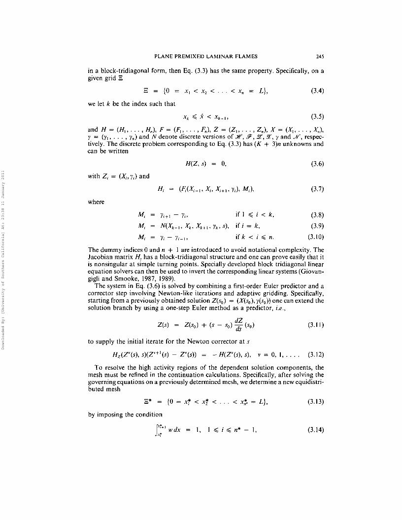
FIGURE 3 A zoom of the flame speed versus 4> response curve for hydrogen-air flames with L = 1m.

structure. First, we note a decrease in the flame temperature 7fand an increase in theflame speed "r- As the equivalence ratio is further increased, the flame speed approaches zero and the flame thickness becomes larger. Ultimately, the flame zone reachesthe downstream boundary x = L and the flame occupies all of the computationaldomain [0, L]. By further increasing the equivalence ratio, the flame is then graduallypressed against the right-hand side of the domain and it is finally extinguished at thatboundary. A turning point in ¢ is then passed and the arclength continuationprocedure proceeds to generate unstable flames until another turning point is passednear ¢ = 0.0. All of the solutions on the lower unstable branch between the twoturning points represent flames pressed against the boundary x = L. Once the secondturning point is passed and the equivalence ratio begins to increase again, the flamemoves away from the right boundary, the reaction zone begins to occupy all of thecomputational domain and eventually the flame thickness decreases and a classicalflame structure is obtained again. Finally, as the equivalence ratio increases further,the stoichiometric conditions are again reached and closed curves are thus obtainedfor (¢, Tf) and (¢,vf)' The lean flammability limit occurred at ¢ = 0.197 withvf = 0.0195 cm/s and 7f = 852.9 K and the rich flammability limit was at ¢ = 11.33with vf = 0.0848 cm/s and T, = 908.3 K. Of course, the computed flame structurescease to be physically relevant as soon as they start to interact with the right boundaryx = L. Observe also that, in general, for plane flames although the response curve(¢, 7f) has two turning points, the response curve (¢, vf) has either very flat turningpoints with d¢/ds = 0, d2¢/di # 0 and dVf/ds # 0 or sometime very flat cusp pointswith dvf/ds = 0, especially at the lean limit.

In order to show the dependence of the extinction points on the size of thecomputational domain [0,L], we have performed another calculation with a value ofL = 10m. The corresponding curve (¢, 7f) is plotted in Figure 4 together with thecurve obtained for L = I m. For this new value of the computational domain, the



'"~ 1500ii!

~~ 1000 ~_----...__--------

~500

15

(",)

20

251

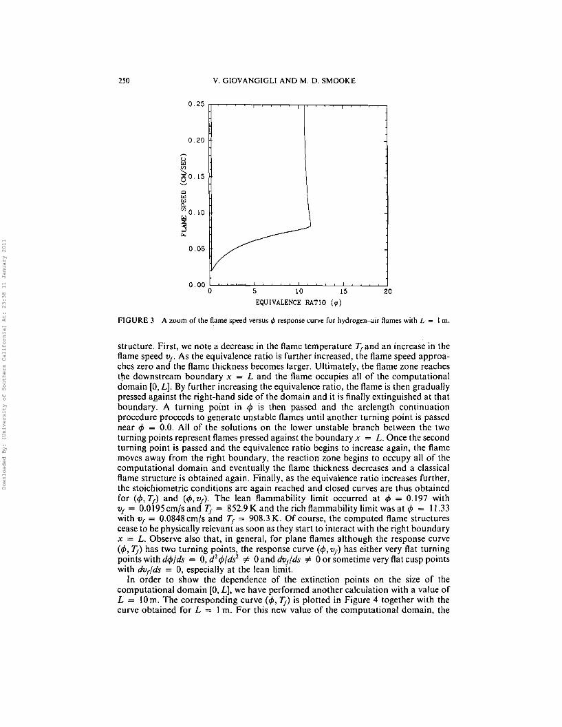
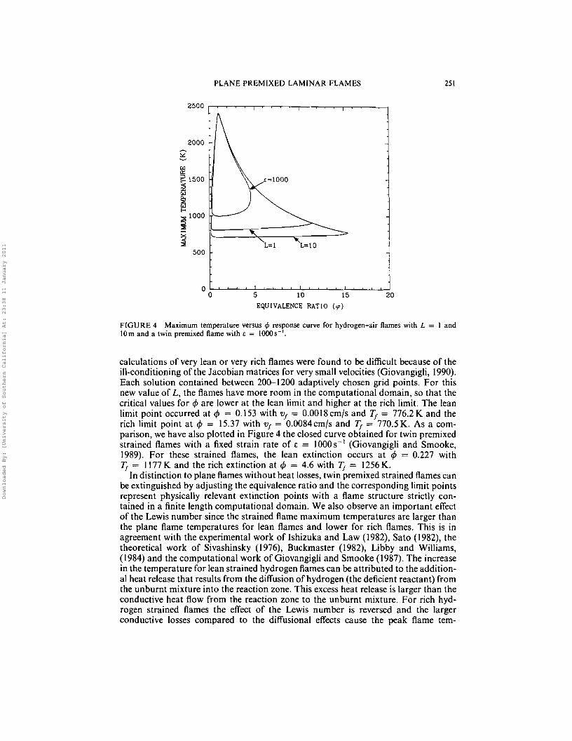
FIGURE 4 Maximum temperature versus e response curve for hydrogen-air flames with L = I and10m and a twin premixed flame with, = 1000s-'.

calculations of very lean or very rich flames were found to be difficult because of theill-conditioning of the Jacobian matrices for very small velocities (Giovangigli, 1990).Each solution contained between 200-1200 adaptively chosen grid points. For thisnew value of L, the flames have more room in the computational domain, so that thecritical values for 4> are lower at the lean limit and higher at the rich limit. The leanlimit point occurred at 4> = 0.153 with vf = 0.0018 cm/s and 1f = 776.2 K and therich limit point at 4> = 15.37 with vf = 0.0084 cm/s and 1f = 770.5 K. As a comparison, we have also plotted in Figure 4 the closed curve obtained for twin premixedstrained flames with a fixed strain rate of E = 1000 S-I (Giovangigli and Smooke,1989). For these strained flames, the lean extinction occurs at 4> = 0.227 with1f = 1177 K and the rich extinction at 4> = 4.6 with 1f = 1256 K.

In distinction to plane flames without heat losses, twin premixed strained flames canbeextinguished by adjusting the equivalence ratio and the corresponding limit pointsrepresent physically relevant extinction points with a flame structure strictly contained in a finite length computational domain. We also observe an important effectof the Lewis number since the strained flame maximum temperatures are larger thanthe plane flame temperatures for lean flames and lower for rich flames. This is inagreement with the experimental work ofIshizuka and Law (1982), Sato (1982), thetheoretical work of Sivashinsky (1976), Buckmaster (1982), Libby and Williams,(1984) and the computational work of Giovangigli and Smooke (1987). The increasein the temperature for lean strained hydrogen flamescan be attributed to the additional heat release that results from the diffusion of hydrogen (the deficient reactant) fromthe unburnt mixture into the reaction zone. This excess heat release is larger than theconductive heat flow from the reaction zone to the unburnt mixture. For rich hydrogen strained flames the effect of the Lewis number is reversed and the largerconductive losses compared to the diffusional effects cause the peak flame tem-



2000

'"~ 1500~

i~ 1000

><~

500

234


5

FIGURE 5 A zoom of the region in Figure 4 containing Lewis number effects.

peratures to decrease with respect to the corresponding plane flames. A zoom of thisregion is illustrated in Figure 5.

In addition to the hydrogen-air flames, we applied the adaptive continuationprocedure to methane-air flames with the pressure equal to one atmosphere,T; = 300 K, and T, = 301 K. A 78 reaction 26 species chemical mechanism (Puri etal., 1987) was used in the calculations and the computational length was L = I m.Starting estimates for the computations were obtained from a procedure similar tothat used in the hydrogen-air flames. Once the initial calculation was completed, theEuler-Newton adaptive continuation procedure was implemented to obtain solutions(physical and unphysical) as functions of the equivalence ratio. The flame temperatureand flame speed response curves (rI>, Tf) and (rI>, vr) are plotted in Figures 6 and 7,respectively. A zoom of the (rI>, vr) response curve is contained in Figure 8. The globalbehavior of the extinction of plane methane-air flames was, in general, similar to thatfor hydrogen-air flames. The lean limit point occurred at 4> = 0.317 with"r = 0.0188cmjs and Tf = 10nK and the rich limit point at rI>= 7.22 with"r = 0.0259 cm/s and Tf = 1181 K. In Figure 9 we illustrate the temperature versusequivalence ratio response curve for the freely propagating premixed flame along witha sequence of temperature versus equivalence ratio curves for twin premixed strainedflames corresponding to fixed strain rates of E = 100, 300, 500, 700, 900, 1100, 1300and 1500s-'. As is clearly illustrated, all the strained flame results fit within the freelypropagating curve. This is consistent with the fact that the Lewis number of methaneis nearly unity throughout the computational domain. In addition, the strained flamesolution manifold forms a hemi-ellipsoid similar to that illustrated in Figure 10. Thestrained curves in Figure 9 correspond to slices of the manifold in Figure lOin the(rI>, T) plane. As the strain rate E --+ 0 and we approach the "wider" opening of theellipsoid, the curves gradually approach the freely propagating premixed case.



10246 8EQUIVALENCE RATIO (~)

500 L-~_--'---_~-----L_~_-'---~_---'--_~_

o

2500

><:>11000

~~~ 1500

~

;;: 2000

FIGURE 6 Maximum temperature versus r/> response curve for methane-air flames with L = I m.

FIGURE 7 Flame speed versus r/> response curve for methane-air flames with L = I m.


254

1.0

0 .8

u

'"en

~O 6

Q

'"'"0..en O. 4

~....l...

0 .2

0.0o

V. GIOVANGIGLI AND M. D. SMOOKE

2 468


10

FIGURE 8 A zoom of the ftame speed versus <I> response curve for methane-air ftames with L = l m,

2500

;;; 2000

~O!~ 1500....

><;: 1000

500o 2 4 6 8


10

FIGURE 9 Maximum temperature versus <I> response curves for methane-air ftames with L = 1m andtwin premixed ftames with s = 100,300,500,700,900, 1100, 1300 and 1500s- 1

•



x

2S5

liE

FIGURE 10 Hemi-ellipsoid solution manifold for the strained premixed laminar flames. The curvelabeled I" denotes the boundary between the physical and unphysical solutions. The curves in Figure 9correspond to slices of the manifold in the (<p, T) plane.

5 CONCLUSIONS

In this paper we have developed a continuation method for the prediction of both leanand rich flammability limits for planar premixed laminar flames. Although thisparticular study focused on adiabatic flames, the method can also be used to predictflammability limits in the presence of heat losses. Of particular importance to thework presented was the generation of a new boundary condition for the energyequation in the unburnt reactant stream. This eliminated the need to specify the valueof a dependent variable (such as the temperature) at some downstream location. Thecontinuation procedure was used to predict the flammability limits for both hydrogen-air and methane-air mixtures in the absence of heat losses. In both cases theflammability limits were shown to be physically irrelevant turning points due to thefinite size of the computational domain, i.e., a different set of flammability limits couldbe determined for a different size of L. In addition, we compared a set of strained twinpremixed laminar flames with each freely propagating case to illustrate the dependence of the peak temperature on the Lewis number of the deficient reactant. As thestrain rate increased, the strained solution curves fit within the closed freely propagating curves thus indicating the hemi-ellipsoidal nature of the solution manifold.

ACKNOWLEDGEMENTS

This work was supported in part by the Office National d'Etude et de Recherches Aerospatiale, the AirForce Office of Scientific Research and the NASA Lewis Research Center. The Centre de Calcul Vectorielpour la Recherche is also acknowledged for Cray CPU time. We would finally like to thank Dr Guy Joulinand Dr. Vincent Borie for a number of interesting discussions concerning this material.

REFERENCES

Bregeon, 8., Gordon, A. S., and Williams, F. A. (1978). Near-limit downward propagation of hydrogenand methane flames in oxygen-nitrogen mixtures, Comb. and Flame 33, 33.

Buckmaster, J. (1982). The quenching of a deflagration wave held in front of a bluff body, SeventeenthSymposium (International} on Combustion, Reinhold, New York. p. 835.

Carter, N. R., Cherian, M. A., and Dixon-Lewis, G. (1982). Flames near rich flammability limits, withparticular reference to the hydrogen-air and similar systems, in Numerical Methods in Laminar FlamePropagation (eds. N. Peters and J. Warnatz), Vieweg.



Gerstein, M. and Stine, W. B. (1973). Analytical criteria for flammability limits, Fourteenth Symposium(International) on Combustion, Reinhold, New York, p. 1109.

Giovangigli, V. and Smooke, M. D. (1987). Extinction of strained premixed laminar flames with complexchemistry, Comb. Sci. and Tech. 53, 23.

Giovangigli, V. and Darabiha, N. (1988). Vector computers and complex chemistry combustion, inProceedings of the Conference on Mathematical Modeling in Combustion, April 1987, Lyon, France,NATO ASI Series.

Giovangigli, V. and Smooke, M. D. (1989). Adaptive continuation algorithms with application tocombustion problems, Appl. Num. Math. 5, 305.

Giovangigli, V, (1990). Mass conservation and singular multicomponent diffusion algorithms, IMPACTCompo Sci. Eng. 2, 73.

Ishizuka, S. and Law, C. K. (1982). An experimental study on extinction and stability of stretched premixedflames, Nineteenth Symposium (International) on Combustion, Reinhold, New York, p. 327.

Joulin, G. and Clavin, P, (1976). Analyse asymptotique des conditions d'extinction des flammes laminaires,Acta Astronaulica 3, 223.

Lakshmisha, K. N., Paul, P. J., Rajan, N. K., Goyal, G., and Mukunda, H. S. (1988). Behavior of methaneoxygen-nitrogen mixtures near flammability limits, Twenty-Second Symposium (International) onComhustion, Reinhold, New York, p. 1573.

Lewis, B. and von Elbe, G. (1961). Combustion. Flames and Explosions of Gases, Academic Press.Libby, P. A. and Williams, F. A. (1984). Strained premixed laminar flames with two reaction zones. Comb.

Sci. and Tech. 37, 221.Lovachev, L. A., Babkin, V. S., Bunev, V. A., V'yun, A. V., Krivulin, V. N., and Baratov, A. N. (1973)

Flammability limits: an invited review, Comb. and Flame 20, 259.Lovachev, L. A. (1979) Flammability limits-a review, Comb, Sci and Tech. 20, 209.Macek, A. (1979) Flammability limits: a re-examination, Comb, Sci and Tech. 21,43.Mayer, E. (1957), A theory of flame propagation limits due to heat loss, Comb. and Flame 1,438.Miller, J. A., Mitchell, R. E., Smooke, M. D., and Kee, R. J. (1982). Toward a comprehensive chemical

kinetic mechanism for the oxidation of acetylene: comparison of model predictions with results fromflame and shock tube experiments. Nineteenth Symposium (International) on Combustion, Reinhold,New York, p. 181.

Miller, J. A., Smookc, M. 0., Green, R. M., and Kee, R. J. (1983) Kinetic modeling of the oxidation ofammonia in flames, Comb. Sci. and Tech. 34, 149.

Peters, N. and Smooke, M. D. (1985). Fluid dynamic-chemical interactions at the lean flammability limit,Comb. and Flame 60, 171.

Puri, i., Seshadri, K., Smooke, M. D., and Keyes, D. E. (1987). A comparison between numericalcalculations and experimental measurements of the structure of a counterflow methane-air diffusionflame, Comb, Sci. Tech. 56, I.

Sato, J. (1982). Effects of Lewis number on extinction behavior of premixed flames in a stagnation flow,Nineteenth Symposium (International) on Combustion, Reinhold, New York, p. 1541.

Sibulkin, M. and Frendi, A. (1990). Prediction of flammability limit of an unconfined premixed gas in theabsence of gravity, Comb. and Flame 82, p. 334.

Sivashinsky, G. J. (1976). On a distorted flame front as a hydrodynamic discontinuity, ACTA Astronautica3,889.

Smooke, M. D. (1982). Solution of burner stabilized premixed laminar flames by boundary value methods,J. Camp. Phys. 48, 72.

Srnooke, M. D., Miller, J. A. and Kee, R. J. (1983). Determination of adiabatic flame speeds by boundaryvalue methods, Comb. Sci. and Tech. 34, 79,

Spalding, D. B. (1957). A theory of inflammability limits and flame-quenching, Proc. Roy. Soc. LondonA240,83.

Strehlow, R. A. (1985). Combustion Fundamentals, McGraw-Hill.Westbrook, C. K. and Dryer, F. L. (1984). Chemical kinetic modelling of hydrocarbon combustion, Prog.

Energy Comb. Sci. 10, I.Williams, F. A. (1985). Combustion Theory, Benjamin/Cummings Pub. Co.Zeldovich, Y. B. (1941). On the quiet flame propagation, Z. Eksp, Tear. Fiz. II, 159.


Combustion Science and Technology Application of ...

Documents

Transcript of Combustion Science and Technology Application of ...