
Combustion in Aviation Gas Turbine Engines of University
140
University of Cape Town The Influence of Fuel Properties on Threshold Combustion in Aviation Gas Turbine Engines Thesis presented for the degree Doctor of Philosophy in the Department Mechanical Engineering University of Cape Town Author: Victor Burger Supervisor: Professor Andrew Yates February 2017
Transcript of Combustion in Aviation Gas Turbine Engines of University

Univers
ity of
Cap
e Tow
n
The Influence of Fuel Properties on Threshold
Combustion in Aviation Gas Turbine Engines
Thesis presented for the degree
Doctor of Philosophy
in the Department Mechanical Engineering University of Cape Town
Author: Victor Burger Supervisor: Professor Andrew Yates
February 2017

The copyright of this thesis vests in the author. No quotation from it or information derived from it is to be published without full acknowledgement of the source. The thesis is to be used for private study or non-commercial research purposes only.
Published by the University of Cape Town (UCT) in terms of the non-exclusive license granted to UCT by the author.
Univers
ity of
Cap
e Tow
n


i
Abstract
This body of work investigated the influence of alternative jet fuel properties on aviation
gas turbine performance at threshold combustor operating conditions. It focused on
altitude blowout performance and was in part motivated by results that were
encountered during an aviation industry evaluation of synthetic kerosene that complied
with the Jet A-1 specification, but differed from the fuel that was used as a reference in
terms of some significant properties. As a consequence the relative impact of physical
properties and reaction chemistry properties were of primary interest in this study.
The thesis considered the potential to blend a range of different alternative jet fuel
formulations which exhibited independent variations in properties relating to
evaporation and reaction behaviour whilst still conforming to legislated physical fuel
specifications. It further explored the potential for said variations having a detectable
and significant influence on the simulated high altitude extinction behaviour in a
representative aviation gas turbine combustor. Based on the findings, appropriate
metrics were suggested for scientifically quantifying the appropriate properties and
conclusions were drawn about the potential impact of alternative jet fuel properties on
blowout performance.
These subjects were addressed primarily through the theoretical analyses of targeted
experimental programmes. The experimental design adopted a novel approach of
formulating eight test fuels to reflect real-world alternative fuel compositions while still
enabling a targeted evaluation of the influences of both physical and chemical reaction
properties. A detailed characterisation was performed of the test fuels’ physical and
reaction properties. The extinction and spray behaviours of the fuels were then
evaluated in a laboratory scale combustor featuring dual-swirl geometry and a single
prefilming airblast atomiser. The various experimental data sets were interpreted within
the context of a theoretical model analysis. In doing so the relative performance of
alternative jet fuel formulations under laboratory burner conditions were translated to
predict relative real world altitude performance. This approach was validated against
aforementioned industry evaluation results and demonstrated to be consistent.
A technically defensible explanation was provided for the previously unexplored
anomalous altitude extinction results that were observed during the industry evaluation
of synthetic jet fuel. A conclusive case was made for the extinction limit differences
having been caused by the relative differences in chemical ignition delays of the fuels.

ii
The probability of volatility (distillation profile) and fuel physical properties playing a
significant role in the impaired altitude performance was discredited. Evaporation-
controlled combustion efficiency was, however, shown to become a significant factor at
low air mass flow rates or when the fuel evaporation is compromised.
The influence of flame speed and chemical ignition delays were investigated. Laminar
flame speed was shown not to correlate with LBO, discrediting its use as a proxy for
reaction rate. The study showed a correlation between the lean blowout behaviour of
jet fuels and the ignition delays associated with their derived cetane numbers.
Additionally, there was substantive support indicating that an even stronger correlation
could be obtained by operating the IQT™ device that is used to measure these delays at
an elevated temperature.
The thesis makes a contribution towards the development of both technical
understanding and practical tools for evaluating the potential operating limits of
alternative jet fuel formulations.

iii
Acknowledgements
I wish to thank the following people:
Professor Andy Yates, for his indispensable guidance, encouragement and
support.
Dr Carl Viljoen for playing a key role in initiating the collaboration with German
Aerospace Centre (DLR) and for trying his best to educate a mechanical engineer
in the dark art of chemistry.
Dr Mariam Ajam and Dr Rina van der Westhuizen for their assistance with the
fuel matrix characterisation.
Sasol Energy Technology, headed by Paul Morgan, for the support and funding of
this project.
The DLR Institute of Combustion Technology, headed Prof. Dr Manfred Aigner,
and especially Dr Thomas Mosbach for hosting me in Stuttgart.
Dr Clemens Naumann for the shock tube ignition delay characterisation of the
test fuels.
Dr William O'Loughlin and Jasper Grohmann, for their assistance during the
model-combustor test measurements.
My parents for their love, support, and patiently explaining organic chemistry and
gas chromatography to me.
This thesis is dedicated to my wife, Zelda, for her love, support, and patience without
which I would not have been able to conclude this work.

iv
Contents
Abstract ................................................................................................................................. i
Acknowledgements ............................................................................................................ iii
List of Figures ...................................................................................................................... vi
List of Tables ........................................................................................................................ x
Acronyms ............................................................................................................................ xi
Nomenclature .................................................................................................................... xii
Subscripts ........................................................................................................................... xiv
1 Introduction ................................................................................................................. 1
1.1 Thesis structure ...................................................................................................... 2
1.2 FSJF certification: Altitude extinction findings ...................................................... 2
2 Preliminary Theoretical Assessment and Project Plan ................................................ 8
2.1 Combustion efficiency ........................................................................................... 8
2.1.1 Evaporation-controlled system ....................................................................... 9
2.1.2 Mixing-controlled system .............................................................................. 11
2.1.3 Reaction-controlled system .......................................................................... 12
2.2 Theoretical flight envelope .................................................................................. 14
2.2.1 Combustion efficiency influences ................................................................. 17
2.3 Hypotheses and project plan ............................................................................... 20
3 Literature Review ...................................................................................................... 23
4 Theoretical Assessment ............................................................................................. 34
4.1 Burning velocity model ........................................................................................ 34
4.2 Stirred Reactor model .......................................................................................... 36
4.3 Evaporation-controlled stability limits ................................................................ 41
4.4 Combustion Efficiencies ....................................................................................... 44
4.4.1 Evaporation-controlled efficiency ................................................................. 44
4.4.2 Mixing-controlled efficiency ......................................................................... 45

v
4.4.3 Reaction-controlled efficiency ...................................................................... 46
5 Experimental Design .................................................................................................. 49
5.1 Test fuel matrix .................................................................................................... 49
5.2 Physical characterisation of test fuel matrix ....................................................... 51
5.3 Chemical characterisation of test fuel matrix ..................................................... 51
5.4 Gas turbine model-combustor: LBO evaluation .................................................. 53
5.5 Gas turbine model-combustor: fuel spray evaluation ......................................... 56
6 Results ........................................................................................................................ 58
6.1 Physical characterisation results .......................................................................... 58
6.2 Chemical characterisation results ........................................................................ 58
6.3 Gas turbine model-combustor: LBO evaluation results ...................................... 64
6.4 Gas turbine model-combustor: fuel spray evaluation results ............................. 66
7 Analysis and Discussion of Results ............................................................................ 69
7.1 Spray and evaporation-controlled system analysis of LBO results ..................... 69
7.2 Reaction-controlled system analysis of LBO results ............................................ 75
7.3 Interpretation of the experimental results .......................................................... 81
8 Summary, Conclusions, and Recommendations ....................................................... 87
Appendix A: Evaporation-controlled System .................................................................. A.1
Appendix B: Comprehensive Fuel Property Analysis Results .......................................... B.1
Appendix C: Shock Tube Ignition Delay Results .............................................................. C.1
Appendix D: PDA Spray Measurement Results ...............................................................D.1
Appendix E: Modelled LBO Air Flow Proportionality Constants ..................................... E.1
References

vi
List of Figures
Figure 1.1: Mach number carpet - Relative performance of AVTUR and SFSAK ................. 4
Figure 1.2: ASTM D86 distillation curves for AVTUR and SFSAK test fuels .......................... 5
Figure 1.3: Lean blowout performance of JP-5 and FSJF relative to Jet A reference fuel ... 6
Figure 1.4: Distillation curves for Jet A, FSJF, and JP-5 test fuels ........................................ 7
Figure 2.1: Evaporation rate curves for kerosene and JP-4 ................................................. 9
Figure 2.2: Comparison of expressions for evaporation efficiency ................................... 11
Figure 2.3: The well-stirred reactor concept ..................................................................... 13
Figure 2.4: Standard atmosphere temperature, pressure and density relative to MSL values ............................................................................................................... 15
Figure 2.5: Typical idealised sub-sonic flight envelope...................................................... 16
Figure 2.6: Theoretical thrust limit, constant evaporation- and reaction-controlled combustion efficiency traces in the altitude-Mach number domain .............. 20
Figure 2.7: Schematic representation of thesis structure ................................................. 21
Figure 3.1: Ignition delay dataset correlation results with D/U and IDT as factors .......... 29
Figure 3.2: Derived cetane number against equivalence ratio at LBO .............................. 30
Figure 3.3: CPT index correlation for diffusion flame extinction ....................................... 31
Figure 3.4: Comparison of DCN to measured LTHR ........................................................... 32
Figure 4.1: Volumetric flow rate vs. efficiency in a typical well-stirred reactor ................ 38
Figure 4.2: Illustrative blowout curves ............................................................................... 39
Figure 4.3: Illustrative blowout curves for Jet A-1 and FSJF .............................................. 41
Figure 4.4: Illustrative reaction and evaporation limited extinction blowout curves ....... 43
Figure 4.5: Extinction performance for simulated wind milling operating condition, schematic representation of the result ........................................................... 43
Figure 4.6: Illustrative timescales in an evaporation limited system with fixed inlet pressure and temperature ............................................................................... 45

vii
Figure 4.7: Illustrative timescales in a mixing limited system with fixed inlet pressure and temperature ..................................................................................................... 46
Figure 4.8: Illustrative timescales in a chemical reaction limited system with fixed inlet pressure and temperature. .............................................................................. 47
Figure 5.1: Laboratory-scale model burner nozzle (configuration B) ................................ 54
Figure 5.2: Laboratory-scale model-combustor layout ..................................................... 55
Figure 5.3: Model-combustor setup .................................................................................. 56
Figure 5.4: Reference Jet A-1 flame ................................................................................... 56
Figure 6.1: Test fuel volatility: distillation profiles. ............................................................ 59
Figure 6.2: Test fuel CJF: Shock tube measured and calculated ignition delay results ..... 61
Figure 6.3: Modelled ignition delay results for the full tests fuel matrix .......................... 62
Figure 6.4: Comparison of IQT™ and shock tube ignition delays ...................................... 63
Figure 6.5: Model-combustor LBO results - burner configuration A, 323 K air pre-heat .. 65
Figure 6.6: Model-combustor LBO results - burner configuration A, 413 K air pre-heat .. 65
Figure 6.7: Model-combustor LBO results - burner configuration B, 323 K air pre-heat .. 66
Figure 6.8: Radial SMD profiles (ɸ = 0.6, 𝑚𝐴 = 6.5 g/s, z = 15 mm from exit plane) ......... 67
Figure 6.9: Radial SMD profiles (ɸ = 0.6, 𝑚𝐴 = 6.5 g/s, z = 35 mm from exit plane) ......... 68
Figure 6.10: Radial SMD profiles (ɸ = 0.6, 𝑚𝐴 = 2.2 g/s, z = 15 mm from exit plane) .. 68
Figure 7.1: Correlation of experimental and theoretical stoichiometric values (effect of proportional representation of configurations A and B) ................................. 74
Figure 7.2: Correlation of experimental and theoretical stoichiometric values (75% configuration B and 25% configuration A) ....................................................... 74
Figure 7.3: Proportionality constants for modelled combustor airflow based on LBO test data - burner configuration B, 323 K air pre-heat ........................................... 76
Figure 7.4: Modified proportionality constants (Kθ) for modelled combustor airflow based on LBO test data - burner configuration A, 323 K air pre-heat ............. 78

viii
Figure 7.5: Modified proportionality constants (Kθ) for modelled combustor airflow based on LBO test data - burner configuration B, 323 K air pre-heat ............. 78
Figure 7.6: Correlation of relative LBO proportionality constants (KAve) and intermediate temperature shock tube ignition delay (ID833 K) .............................................. 81
Figure 7.7: Theoretical relative reaction-controlled extinction limits ............................... 83
Figure 7.8: Theoretical relative evaporation-controlled extinction limits ......................... 84
Figure 7.9: Theoretical relative evaporation- and reaction-controlled extinction limits .. 86
Figure A.1: Evaporation rate curves for kerosene and JP-4 ............................................. A.2
Figure A.2: Drop size vs time ignoring heat-up ................................................................ A.2
Figure A.3: Droplet shell ................................................................................................... A.2
Figure A.4: Comparison of the direct and exponential expressions for evaporation efficiency ......................................................................................................... A.6
Figure C.1: Test fuel CJF: Shock tube ignition delay results .............................................. C.1
Figure C.2: Test fuel CJF/D: Shock tube ignition delay results .......................................... C.1
Figure C.3: Test fuel SJF1: Shock tube ignition delay results ............................................ C.2
Figure C.4: Test fuel SJF2: Shock tube ignition delay results ............................................ C.2
Figure C.5: Test fuel SJF2+: Shock tube ignition delay results .......................................... C.3
Figure C.6: Test fuel LTSK: Shock tube ignition delay results............................................ C.3
Figure C.7: Test fuel HTSK: Shock tube ignition delay results ........................................... C.4
Figure C.8: Test fuel HN: Shock tube ignition delay results .............................................. C.4
Figure D.1: Radial SMD profiles (ɸ = ɸLBO+5%, 𝑚𝐴 = 2.2 g/s, z = 15 mm from exit) ........D.3
Figure D.2: Radial SMD profiles (ɸ = ɸLBO+5%, 𝑚𝐴 = 2.2 g/s, z = 25 mm from exit) ........D.3
Figure D.3: Radial SMD profiles (ɸ = ɸLBO+5%, 𝑚𝐴 = 2.2 g/s, z = 35 mm from exit) ........D.4
Figure D.4: Radial SMD profiles (ɸ = ɸLBO+5%, 𝑚𝐴 = 6.5 g/s, z = 15 mm from exit) ........D.4
Figure D.5: Radial SMD profiles (ɸ = ɸLBO+5%, 𝑚𝐴 = 6.5 g/s, z = 25 mm from exit) ........D.5
Figure D.6: Radial SMD profiles (ɸ = ɸLBO+5%, 𝑚𝐴 = 6.5 g/s, z = 35 mm from exit) ........D.5

ix
Figure D.7: Radial SMD profiles (ɸ = 0.6, 𝑚𝐴 = 2.2 g/s, z = 15 mm from exit) .................D.6
Figure D.8: Radial SMD profiles (ɸ = 0.6, 𝑚𝐴 = 2.2 g/s, z = 25 mm from exit) .................D.6
Figure D.9: Radial SMD profiles (ɸ = 0.6, 𝑚𝐴 = 2.2 g/s, z = 35 mm from exit) .................D.7
Figure D.10: Radial SMD profiles (ɸ = 0.6, 𝑚𝐴 = 6.5 g/s, z = 15 mm from exit) ...............D.7
Figure D.11: Radial SMD profiles (ɸ = 0.6, 𝑚𝐴 = 6.5 g/s, z = 25 mm from exit) ...............D.8
Figure D.12: Radial SMD profiles (ɸ = 0.6, 𝑚𝐴 = 6.5 g/s, z = 35 mm from exit) ...............D.8
Figure E1: Proportionality constants for modelled combustor airflow based on LBO test data - burner configuration A, 323 K air pre-heat .......................................... E.2
Figure E2: Proportionality constants for modelled combustor airflow based on LBO test data - burner configuration A, 413 K air pre-heat .......................................... E.2
Figure E3: Proportionality constants for modelled combustor airflow based on LBO test data - burner configuration B, 323 K air pre-heat .......................................... E.3
Figure E4: Modified proportionality constants (Kθ) for modelled combustor airflow based on LBO test data - burner configuration A, 323 K air pre-heat ............ E.3
Figure E5: Modified proportionality constants (Kθ) for modelled combustor airflow based on LBO test data - burner configuration A, 413 K air pre-heat ............ E.4
Figure E6: Modified proportionality constants (Kθ) for modelled combustor airflow based on LBO test data - burner configuration B, 323 K air pre-heat ............ E.4
x
List of Tables
Table 2.1: International Standard Atmosphere, MSL Conditions ..................................... 15
Table 5.1: Test fuel matrix ................................................................................................ 50
Table 6.1: Test fuel characterisation: key physical properties ......................................... 58
Table 6.2: Test fuel characterisation: GCxGC speciation, DCN, LFS and shock tube ignition delays .................................................................................................. 59
Table 6.3: Correlation analysis of IQT™ and shock tube ignition delay results ................ 64
Table 7.1: PDA spray measurements: Relative SMD values averaged per axial measurement position ..................................................................................... 70
Table 7.2: Average relative effective evaporation constants, SMDs, and evaporation- controlled combustion efficiencies of the test fuel matrix. ............................ 71
Table 7.3: Correlation analysis of relative spray and evaporation metrics and the relative experimental PDA results. ................................................................................ 72
Table 7.4: Correlation analysis of normalised LBO proportionality constants (K) and modified proportionality constants (Kθ) .......................................................... 79
Table 7.5: Correlation analysis of average relative LBO behaviour, fuel spray, LFS and ignition delays .................................................................................................. 80
Table C.1: Arrhenius function coefficients for modelled ignition delay .......................... C.5
Table D.1: PDA spray measurements: Relative SMD values averaged per axial measurement position ....................................................................................D.2
Table E1: Normalised LBO proportionality constants and modified LBO proportionality constants ......................................................................................................... E.1

xi
Acronyms
AFT (p 38) adiabatic flame temperature
ALR (p 18) air/liquid mass ratio
AVTUR (p 3) aviation turbine fuel – reference Jet A-1
CJF (p 49) crude-derived Jet A-1
CJF/D (p 49) crude-derived Jet A-1 + 50% n-dodecane
DCN (p 27) derived cetane number
DEF STAN (p 2) UK defence standard
DLR (p 51) German Aerospace Centre
FAR (p 50) fuel/air mass ratio
FID (p 50) flame ionisation detector
FSJF (p 2) fully synthetic jet fuel
FT (p 48) Fischer-Tropsch
GC (p 50) gas chromatography
GCxGC (p 50) two-dimensional gas chromatography
GTL (p 26) gas to liquids
HCPP (p 49) hydrogenated cat-poly petrol
HTSK (p 49) synthetic paraffinic kerosene (SPK)
HN (p 49) heavy naphtha refinery stream
ICAO (p 14) International Civil Aviation Organisation
ISA (p 14) international standard atmosphere
IQT™ (p 30) ignition quality tester (manufactured by AET, Canada)
LBO (p 1) lean blowout
LFS (p 25) laminar flame speed
LTHR (p 30) low temperature heat release
LTSK (p 49) experimental GTL kerosene
MSL (p 14) mean sea level
NTC (p 59) negative temperature coefficient
OEM (p 2) original equipment manufacturer
PDA (p 50) phase Doppler anemometry
PIV (p 53) particle image velocimetry
SFSAK (p 3) Sasol fully synthetic aviation kerosene (see SJF1)
SJF1 (p 49) FSJF employed during certification process
SJF2 (p 49) commercial FSJF
SJF2+ (p 49) commercial FSJF + 1.5% HCPP

xii
SMD (p18) Sauter mean diameter
SPK (p 26) synthetic paraffinic kerosene
TOF-MS (p 50) time–of–flight mass spectrometry
Nomenclature
Af flame area, [m2]
Aref combustor reference area, [m2]
B constant (eq. 2.7)
d dynamic head, [m]
dyF dimensionless fuel disappearance fraction
dq quench distance, [m]
D instantaneous droplet diameter, characteristic diameter (eq. 4.6) [m]
Da Damköhler number
D0 starting droplet diameter, [m]
DP prefilmer diameter, [m]
Dref width of combustor casing, [m]
D32 Sauter mean diameter, [m]
fc fraction of airflow involved in combustion
𝐺𝑦 axial momentum flux
𝐺𝜃 angular momentum flux
h height above sea level, [km]
H lower specific energy of fuel, [J/kg]
𝑖 reaction order exponent
𝑗 reaction order exponent
K proportionality constant
Kθ modified proportionality constant
K’CJF reaction-controlled proportionality constant for reference fuel CJF
K”CJF evaporation-controlled proportionality constant for reference fuel CJF
𝑙 mixing length, [m]
𝑚 mass of fuel droplet, [kg]
𝑚0 starting droplet mass, [kg]
�̇� rate of fuel evaporation / mass change rate, [kg/s]
�̇�𝑓 rate of fuel evaporation per unit surface area, [kg/m2s]
n number of droplets
�̇� molar air flow rate, [moles/s]

xiii
P pressure, [Pa]
ΔPL combustor liner pressure differential, [Pa]
q fuel/air mass ratio
qref reference dynamic pressure, [Pa]
R gas constant / characteristic radial distance (eq. 5.1)
Re drop Reynolds number
Ru universal gas constant
Sa annular geometric swirl number
Sc centre geometric swirl number
SL laminar flame speed, [m/s]
St small scale turbulent flame speed, [m/s]
ST large scale turbulent flame speed, [m/s]
t time, [s]
te droplet lifetime, [s]
Δtr residence time of air in combustor, [s]
T temperature, [K]
ΔT temperature rise due to combustion, [K]
�̅� rms component of fluctuating velocity, [m/s]
U velocity, [m/s]
Uj turbulent jet velocity, [m/s]
Uref combustor reference velocity, [m/s]
V volume, [m3]
v velocity, [m/s]
𝑥𝐹 fuel mole fraction
𝑥𝑂 oxygen mole fraction
𝑥𝑆 stoichiometric fuel mole fraction
YF overall fuel fraction consumed
α thermal diffusivity
𝜖 turbulent exchange coefficient
ɸ equivalence ratio
λ evaporation constant, [m2/s]
λeff effective evaporation constant, [m2/s]
𝜈 kinematic viscosity, [m2/s]
𝜇 dynamic viscosity, [kg/m.s]
ηc combustion efficiency

xiv
ηe combustion efficiency (evaporation-controlled)
ηm combustion efficiency (mixing-controlled)
ηθ combustion efficiency (reaction-controlled)
τ delay
𝜏𝑐 constant delay offset
τe evaporation timescale
τm mixing timescale
τres residence timescale
τθ reaction timescale
𝜌 density, [kg/m3]
𝜎 surface tension, [kg/s2]
Subscripts
ave average value
A air
c combustion zone value
F fuel
L liquid
ov overall value
(rel) relative to reference value
sl sea level
0 initial value
3 combustor inlet value
1
1 Introduction
Gas turbines dominate aviation propulsion and while they have traditionally always
been considered to be omnivorous fuel consumers, the demands of modern aviation
has resulted in a much more constrained fuel tolerance. Aviation gas turbines need to
operate over a wide range of ambient conditions while attaining ever increasing
efficiency and emission targets. In order to satisfy these demands jet fuel is subjected to
performance-based specifications which have traditionally allowed any combination of
hydrocarbons that satisfied the required performance, provided that they were
petroleum-derived. Significant performance properties include energy content, smoke
point, thermal stability, lubricity, volatility, non-corrosivity and cleanliness. Since the
1940s the specifications have focused predominantly on distillation, volatility, freeze
point, thermal stability and volume yield [1, 2]. In addition, handling and safety
requirements constrain a number of fuel properties. The consequence is that modern-
day aviation fuel is controlled by very explicit specifications that evolved out of a global
industry consensus approach. Environmental and energy security considerations have
stimulated interest in alternatives to petroleum-derived jet fuel which in turn resulted in
an industry-wide review of the complete list of jet-fuel specifications. Sasol played a key
role in this process as the world’s first producer of approved and certified semi-synthetic
and fully-synthetic jet fuels [3].
It is noteworthy that no direct or indirect fuel autoignition specifications are applied to
jet fuel, presumably due to the argument that under normal combustion conditions
chemical reaction timescales are negligible relative to spray vaporization time scales [4].
The combustion performance of practical aircraft combustors is known to be influenced
more by physical processes of heat transfer, mass transfer, thermodynamics, gas
dynamics and fluid dynamics than by chemical processes. While chemical reaction rates
are acknowledged as being of great importance, they are largely disregarded in high
temperature flames due to being considered to be relatively rapid and not rate
controlling. Emphasis is placed on large scale mixing and the interdiffusion of fuel and
air as the rate controlling steps. Chemical processes are, however, known to be of
particular importance for the formation of pollutant emissions and for the lean light-off
and lean blowout (LBO or weak extinction) limits at high flight altitudes [5].
Literature acknowledges the importance of chemical reaction timescales in the
combustion of well atomised fuels at low pressures and lean equivalence ratios as well
as under threshold combustion conditions such as encountered during altitude blowout

Introduction
2
and relight. Increased interest in alternative aviation fuel formulations, and the related
opportunity to influence chemical reaction rates to a greater degree than traditionally
possible in the case of petroleum-derived jet fuel, has prompted examination of the
influence of physical and chemical fuel properties on gas turbine combustion behaviour.
A number of studies have reported ignition and extinction behaviour being influenced
by fuel formulation to varying degrees although it is difficult to separate the influence of
fuel formulation on chemical reaction and fuel evaporation and mixing. These studies
employed experimental setups ranging from laboratory scale combustors to full scale
gas turbines and test fuels ranging from single component fuels to full boiling range jet
fuel formulations. Findings ranged from reports of appreciable differences to relative
insensitivity to fuel formulation [6, 7, 8, 9, 10, 11].
The potential impact of fuel formulation on threshold combustion was also highlighted
by altitude blowout results that were encountered during the evaluation of synthetic
kerosene (Sasol fully synthetic jet fuel or FSJF) as a Jet A-1 aviation turbine fuel under
DEF STAN 91-91 [12, 13].
1.1 Thesis structure
The thesis commences with a summary of the altitude blowout experience that
emerged during the FSJF certification process. This is followed by a chapter entailing a
preliminary theoretical assessment of combustion efficiency and its impact on the flight
envelope. The context of the FSJF results and the theoretical assessment provide the
foundation for the formulation of three thesis hypotheses and the project plan to
address these. A review of relevant literature follows in order to provide context and
background. Based on the guidance provided by the preliminary theory and literature, a
more detailed and focused theoretical assessment is presented. The experimental
design that was formulated to address the hypotheses is presented next. The
experimental results follow as does a subsequent analysis and discussion chapter aimed
at interpreting the results in terms of the hypotheses. Finally some concluding remarks
and recommendations are presented.
1.2 FSJF certification: Altitude extinction findings
During the FSJF certification process, Southwest Research Institute (SwRI) assessed the
results from detailed laboratory testing and submitted the findings to the engine
original equipment manufacturers (OEMs), the British MOD Aviation Fuels Committee,
the Aviation Fuels Group of the Coordinating Research Council, and the ASTM J1
Chapter 1
3
Aviation Fuels Subcommittee. Following the evaluation of the fuel properties and
characteristics, as detailed in a comprehensive report by Moses and Wilson [12], the
OEMs requested engine and combustor tests to confirm no adverse effects on engine
performance and operation. This resulted in a series of test programs being conducted
and or monitored by the OEMs focusing on engine performance, endurance, emissions,
atomisation, ignition and relight, and lean blowout. Moses compiled a report detailing
the results and interpretation of the various engine test programmes, which was
instrumental in the eventual approval of FSJF under DEF STAN 91-91 [13]. The findings
from these test reports contained the following aspects which related specifically to
altitude ignition and extinction.
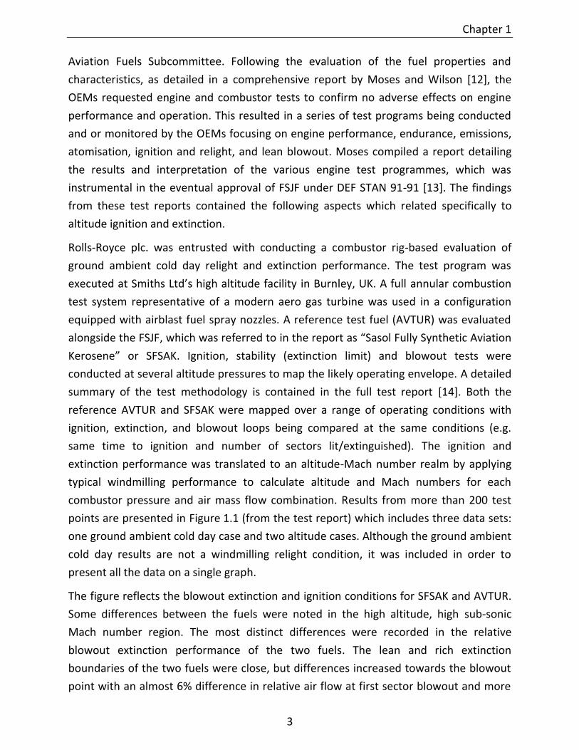
Rolls-Royce plc. was entrusted with conducting a combustor rig-based evaluation of
ground ambient cold day relight and extinction performance. The test program was
executed at Smiths Ltd’s high altitude facility in Burnley, UK. A full annular combustion
test system representative of a modern aero gas turbine was used in a configuration
equipped with airblast fuel spray nozzles. A reference test fuel (AVTUR) was evaluated
alongside the FSJF, which was referred to in the report as “Sasol Fully Synthetic Aviation
Kerosene” or SFSAK. Ignition, stability (extinction limit) and blowout tests were
conducted at several altitude pressures to map the likely operating envelope. A detailed
summary of the test methodology is contained in the full test report [14]. Both the
reference AVTUR and SFSAK were mapped over a range of operating conditions with
ignition, extinction, and blowout loops being compared at the same conditions (e.g.
same time to ignition and number of sectors lit/extinguished). The ignition and
extinction performance was translated to an altitude-Mach number realm by applying
typical windmilling performance to calculate altitude and Mach numbers for each
combustor pressure and air mass flow combination. Results from more than 200 test
points are presented in Figure 1.1 (from the test report) which includes three data sets:
one ground ambient cold day case and two altitude cases. Although the ground ambient
cold day results are not a windmilling relight condition, it was included in order to
present all the data on a single graph.
The figure reflects the blowout extinction and ignition conditions for SFSAK and AVTUR.
Some differences between the fuels were noted in the high altitude, high sub-sonic
Mach number region. The most distinct differences were recorded in the relative
blowout extinction performance of the two fuels. The lean and rich extinction
boundaries of the two fuels were close, but differences increased towards the blowout
point with an almost 6% difference in relative air flow at first sector blowout and more

Introduction
4
than 10% difference in final sector blowout. The SFSAK blowout points occurred at
lower combustor mass flows than those recorded by the AVTUR fuel. This translated
into the significant difference in blowout extinction points of the two fuels in the higher
altitude and Mach number regime of the windmilling envelope shown in Figure 1.1.
Only marginal ignition boundary differences were recorded and were considered to be
within the test method accuracy of 0.005 Fuel-to-Air ratio. The SFSAK toe ignition point
occurred at a 2.5% lower air mass flow than for AVTUR.
Point with lower air mass flow than Toe point; Ignition Toe point for AVTUR;
Ignition Toe point for SFSAK; Blowout point for AVTUR; Blowout point for SFSAK
Figure 1.1: Mach number carpet - Relative performance of AVTUR and SFSAK (from original Rolls-Royce report [14])
The report focused on differences in boiling point distribution between the two fuels
(Figure 1.2) and identified it as a potential cause for the blowout differences. It was,
however, acknowledged that “the possibility of a chemical issue could not be ruled out.”
In light of these results the OEMs recommended further lean blowout tests at lower

Chapter 1
5
altitude conditions that are more relevant to descent where throttle manoeuvres are
expected to be more likely to cause lean combustion.
Figure 1.2: ASTM D86 distillation curves for AVTUR and SFSAK test fuels (from original Rolls-Royce report [14])
In response to the issue raised by Rolls-Royce, Honeywell Aerospace conducted low-
temperature atomisation (at -40°C) and lean blowout tests. The atomisation of the FSJF
was reported to be as good as or better than the Jet A reference fuel for both airblast
and pressure type fuel atomisers. This was ascribed to the lower specific gravity and
viscosity of FSJF and it was concluded that FSJF would provide well-defined spray
distribution and droplet size for reliable cold starting [15]
Lean stability or lean blowout testing was conducted at representative flight and ground
deceleration conditions from sea level up to an altitude of 25000 ft. A full scale reverse-
flow annular combustor rig with dual-orifice fuel atomisers was employed. Three fuels
were evaluated, the FSJF test fuel, Jet A (ASTM D 1655), and weathered JP-5 (MIL-DTL-
5624) which had some volatile components removed and therefore exhibited a flat
distillation profile similar to the FSJF . Blowout points were obtained by reducing fuel
flow after stable combustion had been established. Further detail of the test facility and
measurement procedure is contained in the report.
The results as shown in Figure 1.3 were reported “relative” to those obtained by the
Jet A reference and the authors of the report concluded that lean stability at sea level
was very similar for the three fuels. A “limited fuel effect” was noted at the higher

Introduction
6
simulated altitude (25000 ft.) test point were the FSJF results fell between those
recorded by JP-5 and the Jet A reference. The relative differences were considered to be
small and ordered according to the front-end boiling point distribution of the three
fuels. The distillation curves of the three fuels are presented in Figure 1.4. The JP-5
exhibited a similarly flat distillation profile to that of the FSJF, but while it had the same
flash point the overall distillation was shifted to higher boiling points and the front-end
volatility ranking is apparent. Honeywell concluded that the blowout performance
differences that were reported by Rolls-Royce were not due to chemistry and that FSJF
recorded no adverse effect on combustor lean stability characteristics. The differences
at higher altitude conditions were ascribed to boiling point distribution; volatility and
flash point in particular.
Figure 1.3: Lean blowout performance of JP-5 and FSJF relative to Jet A reference fuel (from original Honeywell Aerospace report [15])

Chapter 1
7
Figure 1.4: Distillation curves for Jet A, FSJF, and JP-5 test fuels (from original Honeywell Aerospace report [15])
While the two studies by Honeywell and Rolls-Royce provided the industry with
sufficient confidence to certify FSJF (with the specified minimum distillation gradient),
the results suggested that the relative influences of physical and chemical properties on
altitude ignition and extinction had not been addressed fully. In order to explore this
subject further it is necessary to first consider the theoretical constraints that apply to
combustion efficiency over the altitude-velocity operating envelope.

8
2 Preliminary Theoretical Assessment and Project Plan
In order to formulate a project hypothesis, it was necessary to subject the results from
the Rolls-Royce and Honeywell Aerospace evaluations to a preliminary theoretical root-
cause analysis. Aviation safety authorities such as the Federal Aviation Administration
and the European Aviation Safety Agency require the submission and validation of so-
called flight envelopes that define the ignition and extinction boundaries of combustion
in an aviation gas turbine. These flight envelopes are essentially the result of the
interplay between atmospheric conditions, hardware design and operation, and
combustion efficiency. In the following section simplified theoretical treatments of
combustion efficiency and flight envelopes are employed to examine the potential for
different fuel properties to influence flight envelope boundaries.
2.1 Combustion efficiency
Gas turbine combustors need to burn stably over a wide range of operating conditions
while maintaining overall combustion efficiencies in excess of 99 percent in order to
meet emissions regulations. Aviation gas turbines furthermore need to ignite readily
after an inflight flameout and attain primary zone combustion efficiencies of 75 to 80
percent as they accelerate back up to normal operation. Lower combustion efficiency
levels could result in rich extinction due to over fuelling in order to overcome the
narrow stability limits at altitude while higher levels could result in an unnecessarily
large combustor [16]. A well-established model for relating combustion efficiency to
combustor operating conditions and dimensions is based on the total time required for
combustion being equal to the sum of the times required for fuel evaporation, mixing of
the reactants (fuel vapour, air and combustion products) and the chemical reaction. The
time available for combustion is inversely proportional to the airflow rate, which means
that the combustion efficiency can be expressed as follows.
𝜂𝑐 = 𝑓 ((𝑎𝑖𝑟𝑓𝑙𝑜𝑤 𝑟𝑎𝑡𝑒)−1 (
1
𝑒𝑣𝑎𝑝𝑜𝑟𝑎𝑡𝑖𝑜𝑛 𝑟𝑎𝑡𝑒+
1
𝑚𝑖𝑥𝑖𝑛𝑔 𝑟𝑎𝑡𝑒+
1
𝑐ℎ𝑒𝑚𝑖𝑐𝑎𝑙 𝑟𝑒𝑎𝑐𝑡𝑖𝑜𝑛 𝑟𝑎𝑡𝑒)−1
) [2.1]
It is understood that under normal conditions the maximum heat release rate is
governed by either evaporation, mixing or chemical reaction rates, but under transient
conditions between either of these regimes the overall combustion efficiency could be
influenced by two of the three concurrently.

Chapter 2
9
2.1.1 Evaporation-controlled system
In a system where the mixing and reaction rates are sufficiently fast for the fuel
evaporation to be the rate-controlling step, the fuel is assumed to instantly mix and
burn with the surrounding air as soon as it evaporates. Under such conditions the
evaluation of evaporation and droplet lifetime is of interest since it determines the
residence time required for combustion to occur. An expanded treatment including all
relevant derivation is included in Appendix A.
The evaporation of a spherical droplet is accepted to consist of an unsteady state or
heat-up period during which the droplet temperature increases with time until the drop
attains its wet-bulb temperature. This transient period is followed by relatively steady-
state evaporation during which the droplet diameter, D, changes according to the so-
called “D2 law of droplet evaporation” that was first formulated by Godsave [17]. Typical
assumptions include: that the droplet is spherical, that the fuel is a pure single boiling
point liquid and that radiant heat transfer is negligible. The mathematical expression of
the law is provided in Equation 2.2 where λ represents the evaporation constant, t the
time elapsed and D and D0 the instantaneous and starting droplet diameters
respectively [18].
𝐷𝑜2 − 𝐷2 = 𝜆𝑡 [2.2]
Figure 2.1 shows this relationship between D2 and time as generated by Wood et al. for
kerosene and JP-4 droplets [19].The fuel-dependent evaporation constant corresponds
to the slope of the linear portion of the graph. During the initial heat-up stage the slope
of the graph is very small while the majority of the heat raises the droplet temperature.
Figure 2.1: Evaporation rate curves for kerosene and JP-4 (from Wood et al. [19])

Preliminary Theoretical Assessment and Project Plan
10
From Equation 2.2 it follows that the evaporation constant, or slope of the curves in
Figure 2.1, are expressed by
𝜆 = 𝑑
𝑑𝑡 (𝐷2) [2.3]
As detailed in Appendix A the average fuel spray evaporation rate �̇�𝑎𝑣𝑒, can be
expressed in terms of the air density 𝜌𝐴, an effective evaporation constant defined by
Chin and Lefebvre [20] λeff, air volume V, fuel/air ratio q, and the initial diameter, D0.
�̇�𝑎𝑣𝑒 = 𝜌𝐴𝜆𝑒𝑓𝑓𝑉𝑞
𝐷02⁄ [2.4]
This expression for average evaporation rate can be employed in determining the
combustion efficiency of a system in which the mixing and reaction rates are sufficiently
fast for the fuel evaporation to be the rate-controlling step. The combustion efficiency is
therefore governed by the ratio of the rate of fuel evaporation within the combustion
zone to the rate of fuel supply.
𝜂𝑒 = �̇�𝑎𝑣𝑒
𝑓𝑐𝑞𝑐�̇�𝐴⁄ [2.5]
The fraction of the total combustor airflow that takes part in combustion is represented
by fc and the combustion zone fuel/air ratio by qc. Substituting 2.4 into 2.5 yields:
𝜂𝑒 = 𝜌𝐴𝜆𝑒𝑓𝑓𝑉
𝐷02𝑓𝑐�̇�𝐴
⁄ [2.6]
Equation 2.6 expresses combustion efficiency in terms of the combustor operating
conditions (𝜌𝐴 , 𝜆𝑒𝑓𝑓 , �̇�𝐴), physical combustor dimensions (V), fuel spray atomiser
properties (D0) and fuel properties (D0 , 𝜆𝑒𝑓𝑓). The equation, however, allows the
evaporation efficiency to assume a value greater than 100%. This occurs when the time
required for complete evaporation is less than the available time and the fuel within the
primary recirculation zone is thus fully vaporised. Under these conditions the
combustion efficiency should be assigned a value of 100%. Lefebvre proposes the use of
a modified form similar to 2.7 in order to avoid the abrupt discontinuity [21]. The two
expressions are compared on the basis of combustion air residence in Figure 2.2. The
value of the shape-function constant, B, is typically chosen so that the efficiency derived
by 2.6 and 2.7 are coincident at the blowout efficiency of around 80%. It should be
noted that 2.7 can over or under predict the base expression 2.6 by up to 15%.

Chapter 2
11
𝜂𝑒 = 1 − exp (−𝐵𝜌𝐴𝜆𝑒𝑓𝑓𝑉
𝐷02𝑓𝑐�̇�𝐴
⁄ ) [2.7]
Figure 2.2: Comparison of the direct (eq. 2.6) and exponential (eq. 2.7) expressions for
evaporation efficiency
2.1.2 Mixing-controlled system
In his treatment of a system where the fuel evaporation and the chemical reaction
kinetics are assumed to be infinitely fast, Lefebvre expressed the combustion efficiency
as a function of the mixing and airflow rate [22].
𝜂𝑚 = 𝑓(𝑚𝑖𝑥𝑖𝑛𝑔 𝑟𝑎𝑡𝑒 𝑎𝑖𝑟 𝑓𝑙𝑜𝑤 𝑟𝑎𝑡𝑒⁄ ) [2.8]
The mixing rate of a turbulent air jet with the gas surrounding it is the product of the
eddy diffusivity, the mixing area, and the density gradient between the jet and the
surrounding gas. By assuming the eddy diffusivity to be proportional to the product of
the mixing length, 𝑙, and the turbulent jet velocity, 𝑈𝑗, the mixing rate can be expressed
as follows:

Preliminary Theoretical Assessment and Project Plan
12
𝑚𝑖𝑥𝑖𝑛𝑔 𝑟𝑎𝑡𝑒 = (𝑒𝑑𝑑𝑦 𝑑𝑖𝑓𝑓𝑢𝑠𝑖𝑣𝑖𝑡𝑦)(𝑚𝑖𝑥𝑖𝑛𝑔 𝑎𝑟𝑒𝑎)(𝑑𝑒𝑛𝑠𝑖𝑡𝑦 𝑔𝑟𝑎𝑑𝑖𝑒𝑛𝑡)
= (𝑙𝑈𝑗)(𝑙2)(𝜌/𝑙)
= 𝜌𝑈𝑗𝑙2 [2.9]
In a combustor where the turbulent jet velocity is a function of the liner pressure
differential, ∆𝑃𝐿, and density: 𝑈𝑗 ∝ (∆𝑃𝐿 𝜌3⁄ )0.5, the mixing rate can be expressed as:
𝑚𝑖𝑥𝑖𝑛𝑔 𝑟𝑎𝑡𝑒 ∝ (𝜌3∆𝑃𝐿)0.5𝑙2
∝ (𝑃3𝑙2 𝑇3
0.5⁄ )(∆𝑃𝐿 𝑃3⁄ )0.5 [2.10]
Substituting the mixing rate expression into 2.8 and assuming the mixing length to be
proportional to the combustor size, 𝐴𝑟𝑒𝑓, the combustion efficiency in a mixing-
controlled system can be expressed as [22]:
𝜂𝑚 = 𝑓 ((𝑃3𝐴𝑟𝑒𝑓 �̇�𝐴𝑇30.5⁄ )(∆𝑃𝐿 𝑃3⁄ )0.5) [2.11]
2.1.3 Reaction-controlled system
There are several theoretical approaches which attempt to characterise combustion
efficiency in a system where chemical kinetics are considered to be rate-controlling and
evaporation and mixing rates are assumed to both be infinitely fast [23, 24, 25]. These
will be examined in greater detail later, but for this preliminary assessment the
commonly used well-stirred reactor provides an adequate representation.
The well-stirred reactor approximates the combustion zone as a perfectly stirred reactor
into which air and fuel flows at a constant rate and the reactants are mixed
instantaneously with all material in the reactor. Combustion products are assumed to
leave the reactor at a constant rate with temperature and compositional properties
identical to that of the reactor or zone. In Lefebvre’s treatment the governing reaction
rate equation (2.12) is presented without explanation [26] as is the case in his
referenced source of this equation, Longwell et al. [27].
𝜂𝑐𝜙�̇�𝐴 = 𝐶𝑐𝑓𝑉𝑇0.5 𝑒(−𝐸 𝑅𝑇⁄ )𝜌𝑛𝑥𝐹
𝑚𝑥𝑂𝑛−𝑚 2.12]

Chapter 2
13
Figure 2.3: The well-stirred reactor concept
A full derivation has, however, been presented by Strehlow [28] based on the
theoretical reactor volume depicted in Figure 2.3. The fuel supply in moles per second is
given by 𝐹𝑢𝑒𝑙 𝑆𝑢𝑝𝑝𝑙𝑦 = 𝜙𝑥𝑠�̇�, where 𝜙 is the molar equivalence ratio, 𝑥𝑠 is the
stoichiometric fuel mole fraction and �̇� is the air flow rate in moles per second.
Assuming a steady flow of premixed reactants into an unstirred reactor, the fuel in
volume element dV is consumed at a rate - 𝑑𝑑𝑡[𝐹]𝑑𝑉 where the fuel concentration, [𝐹], is
the number of fuel moles per unit volume. A dimensionless fuel disappearance fraction,
𝑑𝑦𝐹, can be defined as follows.
𝑑𝑦𝐹 = 𝐿𝑜𝑐𝑎𝑙 𝑓𝑢𝑒𝑙 𝑐𝑜𝑛𝑠𝑢𝑚𝑝𝑡𝑖𝑜𝑛 𝑟𝑎𝑡𝑒
𝑂𝑣𝑒𝑟𝑎𝑙𝑙 𝑓𝑢𝑒𝑙 𝑠𝑢𝑝𝑝𝑙𝑦 𝑟𝑎𝑡𝑒=
−𝑑
𝑑𝑡[𝐹]𝑑𝑉
𝜙𝑥𝑠�̇�
∴ 𝑑
𝑑𝑡[𝐹]𝑑𝑉 = −𝜙𝑥𝑠�̇�𝑑𝑦𝐹 [2.13]
The differential equation can be solved by grouping the variables and integrating over
the reactor volume as well as the fuel consumption profile.
∫𝑑𝑉
𝜙𝑥𝑠�̇�𝑉= −∫
𝑑𝑦𝐹𝑑
𝑑𝑡[𝐹]
𝑌𝐹
0 [2.14]
where the limit, 𝑌𝐹, is the overall fuel fraction consumed. The integral on the right is
difficult to evaluate due to the reaction rate, 𝑑
𝑑𝑡[𝐹], being a function of both
concentration and time. By assuming the reactor to be well-stirred containing a
homogeneous mixture of reactants and products, 𝑑
𝑑𝑡[𝐹] is assumed to be constant
which means that the integration yields:
𝑉
𝜙𝑥𝑠�̇�= −
𝑌𝐹𝑑
𝑑𝑡[𝐹]
[2.15]
∴ 𝑥𝑠�̇�
𝑉= −
1
𝜙𝑌𝐹
𝑑
𝑑𝑡[𝐹] [2.16]
mixture products
dV

Preliminary Theoretical Assessment and Project Plan
14
The reaction rate can be expressed in terms of the fuel and oxidiser concentrations and
an Arrhenius temperature dependence.
Note: Strehlow uses n and m as reaction order coefficients, while Lefebvre uses m and
n-m notation. The fuel and oxidiser reaction order coefficients 𝑖 and 𝑗 are therefore
used here to avoid confusion.
𝑑
𝑑𝑡[𝐹] ∝ −[𝐹]𝑖 [𝑂]𝑗𝑒−𝐸 𝑅𝑇⁄ [2.17]
The initial concentrations of fuel and oxidiser in a constant-volume adiabatic system
may be written as [𝐹] = 𝑥𝐹 𝑃𝑜𝑅𝑢𝑇𝑜
and [𝑂] = 𝑥𝑂 𝑃𝑜𝑅𝑢𝑇𝑜
.
With �̇� ∝ �̇�𝐴 and 𝑌𝐹 ≡ 𝜂𝑐 = 𝜂𝜃, Equation 2.17 into 2.16 results in:
𝜂𝜃𝜙�̇�𝐴 ∝ 𝑉𝑒−𝐸 𝑅𝑇⁄ 𝜌𝑖+𝑗𝑥𝐹
𝑖 𝑥𝑂𝑗
[2.18]
Strehlow omitted a pre-exponential temperature dependence from the Arrhenius
expression which Laidler and Lefebvre included, resulting in the T0.5 discrepancy
between equations 2.12 and 2.18. This is revisited in Chapter 4.
2.2 Theoretical flight envelope
The operating flight envelope of an aviation gas turbine is shaped by atmospheric
conditions, hardware considerations and combustion efficiency limits. Subsonic civil
aircraft operate in the troposphere and lower stratosphere up to typical cruise altitudes
of approximately 38000 ft. (11.5 km) [29]. Knowledge of the vertical distribution of
temperature, pressure, density, viscosity and the speed of sound within the atmosphere
is essential for the modelling of flight conditions. The atmosphere, however, does not
remain constant at any particular place or time which necessitated the development of
a hypothetical approximation known as the standard atmosphere. The International
Organisation of Standardisation (ISO) publishes the International Standard Atmosphere,
ISA, while a number of authorities such as the International Civil Aviation Organisation
(ICAO) and the United States Government publish extensions and subsets of the same
atmospheric model. The models assume the air to be at rest (zero turbulence and no
wind) and to be free of any moisture or dust. Naturally significant differences are
possible between actual atmospheric conditions and the standard atmosphere
properties, which are based on average values recorded at a latitude of 45° N. Table 2.1
provides a summary of the mean sea level (MSL) values employed by the ISA.

Chapter 2
15
Table 2.1: International Standard Atmosphere, MSL Conditions [30]
Temperature Tsl 288.15 K Pressure Psl 101325 N.m-2
Density ρsl 1.225 kg.m-3
Speed of Sound asl 340.294 m.s-1
Gravity gsl 9.80665 m.s-2
Temperature, pressure and density decrease with altitude as shown in Figure 2.4. The
ISA assumes that temperature falls linearly at a rate of 6.5 K/km in the troposphere
below the tropopause (11 km above sea-level). Above 11 km the ISA temperature
remains constant at 216.65 K up to an altitude of 20 km. The pressure, altitude
relationship is given by Equation 2.19 where h is the height above sea-level in km, M is
the molar mass of air and Ru is the universal gas constant. From the ideal gas law density
is given by Equation 2.20.
𝑃 = 𝑃𝑠𝑙 (1 −6.5ℎ
𝑇𝑠𝑙⁄ )
9.81𝑀 6.5𝑅𝑢⁄
[2.19]
𝜌 = 𝑃 𝑅𝑇⁄ [2.20]
Figure 2.4: Standard atmosphere temperature, pressure and density relative to MSL
values

Preliminary Theoretical Assessment and Project Plan
16
A typical sub-sonic flight altitude-Mach number envelope, also sometimes referred to as
a “doghouse plot”, is shown in Figure 2.5. Boundary AB is governed by the minimum
aircraft speed based on either engine thrust or the minimum stall speed. BC is
determined by the operating ceiling of the aircraft and CD is governed by maximum
flight Mach number while DE is determined by the maximum engine thrust. The BCDE
boundary is of particular interest as far as the differences in altitude blowout and relight
behaviour by different fuels are concerned. Although the thermodynamic conditions in
the combustor are strongly influenced by the atmospheric temperature and pressure,
flight speed also plays a significant role as do design parameters such as bypass ratio,
power offtake and exhaust configuration. A simplified approach has been followed to
derive combustor temperatures, pressure and mass flow rates corresponding to the
flight operating envelope.
Figure 2.5: Typical idealised sub-sonic flight envelope
Since the greatest disparity between test fuels in the Rolls-Royce evaluation occurred
under blowout extinction conditions, this condition was simulated in this preliminary
assessment. Conditions prior to in-flight flame-out, or extinction were approximated as
follows. Positions 0, 2, and 3 refer to ambient, compressor inlet, and compressor outlet
positions respectively. For a given compressor ratio, 𝑟 = 𝑃3 𝑃0⁄ , the isentropic
temperature ratio from the compressor inlet to combustor inlet is given by:

Chapter 2
17
𝑇3is
𝑇2= 𝑟(𝛾−1) 𝛾⁄ [2.21]
Isentropic compressor efficiencies in modern aircraft gas turbines are typically around
90% [31] and treating the fluid as an ideal gas it can be expressed as
𝜂𝑐𝑜𝑚𝑝 = 𝑇3is− 𝑇2
𝑇3− 𝑇2 [2.22]
The actual temperature ratio over the compressor is thus given by
𝑇3
𝑇2= 1 +
𝑟(𝛾−1) 𝛾⁄ − 1
𝜂𝑐𝑜𝑚𝑝 [2.23]
The stagnation pressure can be calculated via the isentropic relationship
𝑃0 = 𝑃 (1 +𝛾−1
2𝑀2)
𝛾 (𝛾−1)⁄
[2.24]
2.2.1 Combustion efficiency influences
Boundary BCDE in Figure 2.5 can be impacted by combustion efficiency and therefore
fuel influences on combustion efficiency can potentially also delimit the envelope
boundary. This potential impact was investigated by applying the modelled evaporation-
mixing- and reaction-controlled efficiency expressions to the idealised altitude, Mach
number model. Physical hardware parameters and proportionality constants were
arbitrarily chosen to illustrate potential envelope limits. The mixing-controlled efficiency
as defined in Equation 2.11 is insensitive to flight conditions and does not impact
boundary BCDE. This is revisited in Chapter 4.
Equation 2.6 was employed to model the evaporation-controlled efficiency over the
operating altitude temperature, pressure, and air mass flow range.
𝜂𝑒 = 𝜌𝐴𝜆𝑒𝑓𝑓𝑉
𝐷02𝑓𝑐�̇�𝐴
⁄ [2.6]
Combustion efficiencies of at least 75 to 80% are required to sustain combustion and
prevent flameout [16]. A combustion efficiency limit of 75% was therefore used to
calculate the corresponding maximum flight Mach numbers. Chin and Lefebvre [20]
presented plots of effective evaporation constants versus boiling point for various
values of droplet size and velocity at three pressures and three ambient temperatures.
They acknowledged that while a single fuel property cannot fully describe evaporation
characteristics of any given fuel, average boiling point has the benefit of being directly

Preliminary Theoretical Assessment and Project Plan
18
related to vapour pressure and fuel volatility. Using these three plots, Equation 2.25 was
derived empirically for calculating the effective evaporation constant. The omission of
droplet size and velocity was deemed to be an acceptable simplification for an initial
investigation. The fuel boiling point was treated as constant for a single fuel model and
is revisited in Section 7.3 for the evaluation of multiple fuels with variable boiling point
temperatures.
𝜆𝑒𝑓𝑓 ∝ 𝑃0.09 𝑇1.8 [2.25]
The majority gas turbines employ prefilming airblast atomisers combined with strong
swirling flow to ensure fine atomisation and dispersion of droplets throughout the
combustion zone. Rizkala and Lefebvre [32] concluded that for fluids such as kerosene
with relatively low viscosities the mean droplet size is primarily influenced by surface
tension, air velocity and air density while viscosity plays and independent role. They
proposed a two-term expression for Sauter mean diameter, SMD, (Equation 2.26) based
on analysis of experimental data where the first term is dominated by surface tension
and air momentum and the second by liquid viscosity. Lefebvre subsequently presented
a modified version (Equation 2.27) with experimentally determined burner-specific
constants A and B [33].
𝑆𝑀𝐷 = 3.33 × 10⁻³(𝜎𝜌𝐿𝐷𝑃)
0.5
𝜌𝐴𝑈𝐴(1 +
1
𝐴𝐿𝑅) + 13.0 × 10⁻³ (
𝜇𝐿2
𝜎𝜌𝐿)0.425
𝐷𝑃0.575 (1 +
1
𝐴𝐿𝑅)2
[2.26]
𝑆𝑀𝐷 = 𝐴 (𝜎
𝜌𝐴𝑈𝐴2𝐷𝑃)0.5
(1 +1
𝐴𝐿𝑅) + 𝐵 (
𝜇𝐿2
𝜎𝜌𝐿𝐷𝑃)0.5
(1 +1
𝐴𝐿𝑅)2
[2.27]
DP is the prefilmer diameter, 𝑈𝐴 the air velocity, and ALR the air/liquid mass ratio. For
low viscosity liquids such as water and kerosene the first term predominates resulting
in 2.28.
𝑆𝑀𝐷 = 𝐷32 ∝ (𝜎
𝜌𝐴𝑈𝐴2𝐷𝑃)0.5
(1 +1
𝐴𝐿𝑅) [2.28]
With 1 +1
𝐴𝐿𝑅≈ 1 +
𝜙
14.6≈ 1 and assuming constant hardware dimensions as well as fuel
properties, Equation 2.6 simplifies to:
𝜂𝑒 ∝ 𝑃1.09𝑇0.8 / �̇�𝐴 [2.29]
Applying the atmospheric pressure and temperature values at varying altitude, and
setting the blowout threshold evaporative efficiency at a fixed 75%, one obtains the
theoretical evaporation-controlled limit curve as is shown in Figure 2.6. Note that the

Chapter 2
19
value of the proportionality constant was arbitrarily chosen for illustration purpose so
that the limit contour passed through Mach 0.87 at an altitude of 10 km.
The reaction-controlled combustion efficiency was based on Equation 2.18 and the
assumption that for an overall global reaction scheme the fuel and oxygen
concentrations could be regarded as referring to the initial concentrations 𝑥𝐹 = 𝜙
𝜙+85.7
and 𝑥𝑂 = 18
𝜙+85.7. With 𝜙 < 1 both 𝑥𝑂 and the denominator of 𝑥𝐹 are nominally
constant and can be absorbed into the overall proportionality. Equation 2.18 therefore
simplifies to 2.30 and employing exponents of 𝑖 and 𝑗 corresponding to the values
recommended by Lefebvre [24], the efficiency expression can be further reduced to
2.31. This was employed to produce the theoretical reaction-controlled extinction limit
contained in Figure 2.6. Again, the overall proportionally constant was arbitrarily chosen
for illustrative purpose only.
𝜂𝜃𝜙�̇�𝐴 ∝ 𝑉𝑒−𝐸 𝑅𝑇⁄ 𝜌𝑖+𝑗 𝜙𝑖 [2.30]
𝜂𝜃 ∝ 𝑉𝑒−𝐸 𝑅𝑇⁄ 𝜌1.75 �̇�𝐴⁄ [2.31]
The broken curves parallel to the evaporation and reaction-controlled curves are
illustrative of the effect that variations in the proportionally constants have, as would be
expected for different fuels with different evaporation and reaction behaviour.
A number of conclusions were drawn from the theoretical treatment and resultant
Figure 2.6. The mixing-controlled limit is independent of the air flow and air density (to a
first order of magnitude analysis), which discounts it from playing a role in the
discrepancy that Rolls-Royce detected at high altitude and high subsonic Mach numbers.
This is further reinforced by the fact that fuel properties do not directly influence the
parameters contained in the equation governing mixing behaviour (2.11).
The negative gradient of both the evaporation and reaction-controlled limits suggest
that either of these aspects could provide a candidate explanation for the fuel-related
variance that was detected by Rolls-Royce. The fact that fuel properties could
conceivably cause a significant distinction in the manifestation of either of these limiting
efficiency boundaries does not contribute to determining the more probable candidate.
The theoretical treatment is supported by the Honeywell Aerospace test results which
detected very little distinction between the different test fuels. These tests were

Preliminary Theoretical Assessment and Project Plan
20
conducted at 25000 ft. (7.62 km) where the flight envelope is not expected to be
governed by fuel properties.
Figure 2.6: Theoretical thrust limit, constant evaporation- and reaction-controlled combustion efficiency traces in the altitude-Mach number domain
Chapter 4 revisits the efficiency limit treatments in terms of fluid-mechanic and
chemical timescales to examine their relevance under the different combustor
conditions and with different fuels.
2.3 Hypotheses and project plan
The preceding preliminary theoretical treatment identified the root cause of the altitude
blowout differences by the Rolls-Royce report as being determined by either the
evaporation or the reaction-controlled combustion efficiency but not by mixing
efficiency. The following three hypotheses were therefore formulated to define the
scope of the thesis:
Hypothesis 1: A range of aviation jet fuels could be blended according to a design-of-
experiment strategy to exhibit independent variations in properties relating to
evaporation and reaction behaviour whilst still meeting the legislated physical fuel
specifications.

Chapter 2
21
Hypothesis 2: The range of variations contemplated in Hypothesis 1 could have a
detectable and significant influence on the simulated high altitude extinction behaviour
in a representative aviation gas turbine combustor. (Note that this is not a legislated
criterion)
Hypothesis 3: The relevant properties described in Hypothesis 1 can be scientifically
quantified in an appropriate test apparatus and can be correlated to the high-altitude
extinction behaviour described in Hypothesis 2.
The thesis was structured to address these hypotheses primarily through theoretical
analyses of targeted experimental programmes. A schematic summary of the thesis
structure is presented graphically in Figure 2.7.
Figure 2.7: Schematic representation of thesis structure with relevant section numbers
provided in brackets.

Preliminary Theoretical Assessment and Project Plan
22
The evaporation and chemical reaction properties of the test fuels were assessed
against theoretical models prior to being incorporated in the evaluation of the
experimental results. Theoretical models were presented of both evaporation and
reaction limited combustion. The theoretical models, fuel properties and results from
model-combustor experiments were combined to interrogate evaporation and reaction-
controlled extinction behaviour and address hypotheses 1 and 3. By combining these
results with a theoretical analysis of higher altitude and Mach number operation,
Hypothesis 3 was addressed and an explanation was provided for the results of the FSJF
certification tests.
In the following sections a selection of relevant literature is reviewed prior to the
theoretical assessment being expanded in support of the experimental design and
evaluation of test results.

23
3 Literature Review
The combustion performance of practical aircraft combustors is known to be primarily
influenced more by physical processes of heat transfer, mass transfer, thermodynamics,
gas dynamics and fluid dynamics than by chemical processes. While chemical reaction
rates are acknowledged as being of great importance they are largely disregarded in
high temperature flames due to being considered to be relatively rapid and not rate
controlling. Emphasis is placed on large scale mixing and the interdiffusion of fuel and
air as the rate controlling steps. Chemical processes are, however, acknowledged to be
of particular importance for the formation of pollutant emissions and for the lean light-
off and lean blowout (or weak extinction) limits at high flight altitudes [4, 5].
The difficulty in investigating fuel property effects on gas turbine combustion is evident
throughout literature. The interrelated nature of various fuel properties precludes the
classical experimental research approach of quantifying the effects of varying a single
independent parameter while maintaining all others relatively constant. The fact that
different hardware designs have been shown to respond differently to fuel property
variations is a further confounding factor. One notable example can be found in the
response of liner temperature of combustors with either lean or rich primary
combustion zones to carbon/hydrogen (C/H) ratio variations. Heat transfer to the liner
wall is primarily due to radiation in the case of rich primary zone combustion and is thus
governed by flame emissivity, which in turn is influenced by the C/H ratio. In a lean
primary combustion zone heat transfer to the liner wall occurs primarily due to forced
convection which is relatively insensitive to C/H ratio changes with the gas temperature
being dominant [34].
In many instances engine-hardware-oriented studies that focused on investigating the
influences of gas turbine fuel properties on combustion analysed the net effect of fuel
variations on a specific combustor parameter. In some instances attempts were made to
isolate and categorise fuel property effects.
Venkataramani isolated fuel volatility effects from atomisation effects during an
investigation of fuel property influences on altitude relight performance [35]. The study
focused only on separating the influences of physical fuel properties, while chemical
property differences were not investigated. Four test fuels were employed (JP-4, Jet A,
Jet A/2040 solvent blend, and Diesel 2) covering a wide range of volatilities. In order to

Literature Review
24
eliminate fuel specific effects on atomisation, injection equipment was used that
maintained equivalent SMD values (50 ± 10 μm) for all test fuels at equal design flow
rates. The results revealed, inter alia, that fuel volatility assumed a secondary role in
initial (first cup) light-off. Decreased volatility resulted in slightly poorer blowout
performance but full-propagation and first cup blowout were found to be independent
of fuel volatility. In spite of the previously mentioned acknowledgement that chemical
reaction time scales can be significant under threshold conditions such as encountered
during altitude relight, the potential influence of the fuels exhibiting different chemical
reaction rates was not taken into account. Airblast atomisers were shown to exhibit
poorer ignition performance and a stronger volatility dependence than pressure
atomisers.
In another investigation aimed at anticipating the combustion performance effects of
future fuel formulations, Lefebvre analysed a large body of data from studies conducted
by the USAF, Army, Navy and NASA [34]. The matrix of thirteen test fuels included JP-4,
JP-8, five blends each of JP-4 and JP-8, as well as a No. 2 diesel which provided three
levels of hydrogen content: 12, 13 and 14 percent by mass. The results from the studies
were analysed to determine how combustion efficiency, lean blowout limits, ignition
performance, liner wall temperature, emissions and pattern factor were influenced by
the differences in fuel formulation.
Hydrogen content and/or aromatic content exhibited a significant influence on flame
radiance, liner wall temperature and smoke emissions. Physical fuel properties that
influenced atomisation quality and evaporation rates were shown to affect lean
blowout, ignition, combustion efficiency and CO emissions while liner wall temperature,
NOx and smoke emissions were not influenced by fuel physical properties. Combustion
efficiency, lean blowout, ignition and CO and NOx emissions exhibited a small
dependence on fuel chemistry differences. This was attributed to the influence of slight
variations in calorific value on combustion temperature. The physical fuel properties had
an appreciable effect on pattern factor at low power conditions but this effect
decreased to be very small at high power settings where pattern factor effects on vane
life are typically most significant. The combustor pattern factor was not influenced by
fuel chemistry. It should be noted that in this study the carbon to hydrogen (C/H) ratio
was taken as representative of the fuel chemistry differences and no metric

Chapter 3
25
representative of chemical reactivity such as ignition delay or laminar flame speed (LFS),
was measured or reported.
Rao and Lefebvre [36] concluded that the presence of sufficient fuel vapour in the
ignition zone is the sole determining criterion for ignition of heterogeneous mixtures of
fuel droplets in air. Ignition will ensue automatically if sufficient thermal energy is
created by the passage of the spark to produce the required amount of fuel vapour. The
basis of this argument is the understanding that, over a wide range of operating
conditions, the chemical reaction time is very short relative to the time required for
producing an adequate amount of fuel vapour in the ignition zone. This is, however, not
necessarily the case under threshold conditions where the reaction timescales can be
impaired.
Ballal and Lefebvre [37] proposed theoretical models for determining the minimum
ignition energy required and the quench distance in liquid fuel sprays. Quench distance
is defined as the critical spark-kernel size at which the rate of heat loss at the kernel
surface is equal to the rate of heat release throughout the kernel volume, due to the
instantaneous combustion of fuel vapour. The kernel must attain this size in order for
combustion to propagate unaided and the minimum ignition energy is defined as the
amount of energy required from an external source to attain the quenching distance [4].
In a subsequent study the model was extended to include the presence of fuel vapour in
the mixture entering the ignition zone and the influence of finite chemical reaction
rates, which are known to be significant for well atomised fuels at low pressures and low
equivalence ratios [38]. This yielded Equation 3.1 for calculating quenching distance (dq)
for all conditions likely to be encountered in practical combustion systems. A good fit
was obtained with experimental data over SMD values ranging from 40 to 150 μm.
𝑑𝑞 = [𝜌𝐹𝐷32
2
𝜌𝐴𝜙𝑙𝑛(1+𝐵𝑠𝑡)+ (
10𝛼
𝑆𝐿)2
]0.5
[3.1]
The first term of the root sum square equation deals with fuel evaporation. Fuel and air
densities are represented by ρF and ρA respectively, Sauter mean diameter by D32,
equivalence ratio by ɸ, and the stoichiometric mass transfer number by Bst. The second
term introduces a measure of a fuel chemistry influence with α representing the
thermal diffusivity and SL the laminar flame speed of the fuel. By dividing the thermal
diffusivity by the laminar flame speed, the second term effectively reduces to the

Literature Review
26
product of the specific heat at constant pressure (Cp), density (ρ) and laminar flame
thickness ( L ). The influence of the chemical reaction rate is thus reflected in terms of
the laminar flame thickness. The importance of chemical reaction timescales in the
combustion of well atomised fuels at low pressures and lean equivalence ratios as well
as under threshold combustion conditions such as encountered during altitude relight
and blowout is therefore acknowledged to some degree.
Increased interest in alternative aviation fuel formulations, and the related opportunity
to influence chemical reaction rates to a greater degree than traditionally possible in the
case of petroleum-derived jet fuel, has prompted investigation into the influence of
physical and chemical fuel properties on gas turbine combustion behaviour. A number
of recent studies have reported ignition and extinction behaviour being influenced by
fuel formulation to varying degrees. These studies employed experimental setups
ranging from laboratory scale combustors to full scale gas turbines and test fuels
ranging from single component fuels to full boiling range jet fuel formulations. Findings
ranged from reports of appreciable differences to relative insensitivity to fuel
formulation [6 - 13].
Fyffe et al. conducted an altitude ignition and extinction evaluation of five synthetic
paraffinic kerosene (SPK) fuel formulations at the Rolls-Royce plc. sub-atmospheric
altitude ignition facility in Derby, UK [8]. A multi-sector representation of an advanced
gas turbine combustor and fuel injector was used to evaluate threshold combustion at
two test conditions that were considered to be representative of approximate altitude
conditions of 25000 to 30000 ft. (7.62 to 9.14 km). The five test fuels were all GTL-
derived and were compared against a representative crude-derived Jet A-1. The results
were interpreted against three compositional variables that were chosen to define the
fuel matrix: carbon number distribution (narrow vs. wide), iso/normal paraffin ratio and
total paraffinic content. Unfortunately other fuel properties were not reported which
hinders the subsequent critical assessment of the results. Some differences were
reported in ignition behaviour but extinction differences were considered to be within
the experimental scatter. The study associated low iso/normal paraffin ratios with
improved ignition behaviour. This trend is known very well in diesel and gasoline engine
fields where the extremities of the respective cetane and octane rating scales are each
defined by a normal and iso-paraffinic reference fuel. The results were not subjected to
a theoretical assessment and fundamental reasons for the observed behaviour were not

Chapter 3
27
offered but it did support the possibility for fuel formulation differences impacting
threshold combustion.
Burger et al. presented results from a lean blowout (LBO) study of 16 different fuel
formulations in an in-house developed combustor that was based on the primary zone
of an Alison T63. A simplex pressure atomiser nozzle was used in the evaluation. The
authors reported blowout limits correlating with volatility and significantly reported a
(weak) negative correlation between derived cetane number (DCN) and LBO [7].
A follow-on paper evaluated eight test fuels from the same matrix in a representative
aero-engine combustor sector equipped with an airblast atomiser [9]. Significant
variability in the results prevented more definitive conclusions being drawn from this
study. It is notable that the shape of the extinction limit curves suggests that the tests
were conducted in a regime that was primarily influenced by evaporation efficiency. It is
significant that under this regime of operation any potential correlation between DCN
and LBO was masked. This topic is revisited in more detail under Section 4.3.
Rock et al. reported on an experimental study of lean blowout in a swirl-stabilised
combustor equipped with both pressure and airblast atomisers [10]. The study’s key
motivation was similar to this thesis, to investigate the relative roles of physical
properties and chemical kinetic properties on lean blowout behaviour. The test fuel
matrix encompassed eight fuels including three crude-derived jet fuels (Jet-A, JP-5, and
JP-8) and five formulations that spanned a range of physical and chemical properties.
The pressure atomiser blowout tests revealed strong correlations with fuel physical
properties, particularly boiling point temperature. Fuels that were less easily atomised
and vaporised were harder to blowout. This is in accordance with the concept that
delaying atomisation and or vaporisation delays the level of premixing that drives very
lean global fuel-air ratios. It creates localised regions of higher fuel-air ratios and
elevated flame temperatures which supports combustion. The authors proposed that
this behaviour was dependent on the pre-heat temperature being above the fuel flash
point and that the reverse behaviour is exhibited when the pre-heat temperature is
lower than the flash point which would be in agreement with the work by
Burger et al. [7]. It also agrees with the statement by Lefebvre that pressure atomisers
typically produce lower fuel/air mixing prior to combustion and have superior blowout
performance [39]. With the exception of one fuel, the pressure atomiser results also
reported good correlations between blowout and C/H ratio, iso-paraffinic content and

Literature Review
28
fuel smoke point. The authors ascribed this to a strong co-correlation with the more
significant physical parameter T90.
In contrast to the pressure atomiser behaviour, Rock et al. reported no strong
correlation between the blowout behaviour recorded with the airblast atomiser and fuel
physical properties. The strongest correlation that they recorded was with the iso-
paraffinic content of the test fuels which the authors ascribed to being driven by the
chemical kinetic properties of the fuel. The authors indicated that no clear correlation
was found between the airblast blowout results and cetane number which was
supported by substantial scatter in the figures presented. However, closer inspection of
the correlation matrix revealed significant negative correlations with LBO for both
atomiser options. This was further supported by a strong negative correlation between
iso-paraffinic content and cetane numbers. This lacuna within the paper is significant in
view of the contradictory observations highlighted in the earlier works. It is especially
relevant to the present research initiative and provides a motivation for a careful study
of the issue of a possible correlation between the cetane rating of the fuel and LBO.
Grohmann et al. investigated lean blowout differences using the same gas turbine
model-combustor that was employed in this thesis [11]. In an attempt to minimise the
complexity inherent in multi-component jet fuel, they selected six single-component
model fuels to represent normal, branched, cyclic and aromatic hydrocarbons. The
paper reported atomisation, vaporisation, chemical kinetic properties and lean blowout
results for three of these fuels: n-hexane, n-dodecane and iso-octane. The authors
observed that both physical and chemical fuel properties influenced the measured LBO
behaviour. Differences in the LBO behaviour of n-hexane and iso-octane were ascribed
to chemical kinetic nature of the fuels and in agreement with normal alkanes exhibiting
shorter ignition delays than branched alkanes (of the same carbon number). The two
fuels exhibited very similar atomisation and vaporisation behaviour.
By comparison n-hexane and n-dodecane revealed comparable chemical kinetic
characteristics, but very different atomisation and vaporisation behaviour. At high air
pre-heat temperatures the two fuels reported similar LBO results, but at lower pre-heat
the larger droplets and lower evaporation rate of n-dodecane was credited with
extending LBO limits. The authors proposed a similar explanation to that offered by
Rock et al. [10] but interestingly in this instance the atomiser was a prefilming airblast
unit.

Chapter 3
29
Bluff-body flames have been studied extensively, but a lack of consensus about the
physical and chemical processes that lead to blowout motivated a study by Heulskamp
et al. which utilised a large data set of experimental and literature LBO results for bluff-
body stabilised flames to develop a correlation for predicting lean blowout [40]. They
confirmed a dependence on the Damköhler number with fuel variation playing a
significant role. Damköhler number is commonly used in chemical engineering as an
expression of the ratio of chemical and fluid-mechanic timescales. Most researchers
agree that LBO is governed by it, but there have been different proposals about the
definition of the critical timescales. Research such as reported by Shanbhogue et al.
advocate the impact of ignition delay while Radhakrishnan et al. and Kariuki et al.
presented successful correlations with flame speed which argued that blowout is not
governed by ignition timescales [41, 42, 43].
Heulskamp et al. thus endeavoured to provide clarity about critical parameters and their
significance to physical and chemical processes. They concluded that pressure,
temperature and C/H ratio of the fuel impacted the reactivity of the mixture and
contributed to the chemical timescale within the Damköhler number. It was confirmed
that blowout was not solely dependent on the fluid mechanic timescales and LFS was
discredited as a blowout predictor. Ignition delay was found to be an excellent
representation of the chemical timescale in the experimental data set as evidenced by
Figure 3.1 where D/U refers to the fluid-mechanic timescale (U is the lip velocity and D is
the characteristic diameter of the bluff body).
Figure 3.1: Ignition delay dataset correlation results with D/U and IDT as factors
(R2 = 0.918) (from Heulskamp et al. [40])

Literature Review
30
The authors also advocated the influence of cetane number and C/H ratio on blowout
behaviour due to the covariance of these properties with ignition delay. This is in
agreement with Colket et al. who reported fuels with higher cetane numbers and higher
C/H ratios blowing out at lower equivalence ratios as shown in Figure 3.2 [44].
Figure 3.2: Derived cetane number against equivalence ratio at LBO
(from Colket et al. [44])
The work by Won et al. [45] also supported the relevance of cetane number to gas
turbine combustion and extinction. Their study of the pre-vaporised global combustion
behaviour of a selection of petroleum-derived and alternative jet fuels yielded a
‘‘combustion property target (CPT) index” that was developed through regression
analysis of results from three experiments. The CPT index was proposed as a fuel
screening tool for assessing fully pre-vaporized, kinetically coupled behaviours of
potential alternative jet fuel formulations. Derived cetane number (DCN) was included
in the analysis as a measure of autoignition propensity. DCN is calculated directly from
ignition delay measurements in an ignition quality tester (IQT™) which will be discussed
in greater detail under the experimental design in Chapter 5. The resultant CPT index for
extinction employed DCN, heat of combustion, and molecular weight and the CPT index
for low temperature heat release (LTHR) rate was purely based on DCN. Figure 3.3
reproduces a figure reporting the results of the linear regression of the diffusion flame

Chapter 3
31
extinction at a fixed mass fuel fraction (Yf = 0.4). The typical range of JP-8 fuels is
demarcated by the dashed rectangle.
Figure 3.3: CPT index correlation for diffusion flame extinction at Yf = 0.4
(from Won et al. [45])
Figure 3.4 provides a comparison of DCN and the measured LTHR rate as represented by
the maximum H2O mole fraction in the temperature range between 550 and 700 K.
The authors made the pertinent comment about DCN in the context of LTHR that most
of the alternative jet fuels and their blends with petroleum-derived jet fuels were
outside of the variability of JP-8. In light of the approval of 50:50 blends of SPK and
crude-derived fuel they made the point that low temperature reactivity might not be a
critical combustion property for existing gas turbines. However, they highlighted that
advanced engine designs are focused on increasing pressure ratios and combustor
pressures significantly in order to achieve greater efficiency. Under these conditions low
temperature reactivity is expected to play a more significant role under threshold
combustion conditions such as LBO and altitude relight.

Literature Review
32
Figure 3.4: Comparison of DCN to measured LTHR (from Won et al. [45])
Evidence from literature clearly supports the importance of considering both physical
and chemical fuel properties in the context of threshold combustion and high altitude
blowout extinction. There are, however, inconsistencies and omissions in said literature
which necessitate further exploration.
One example is the contradicting conclusions regarding the impact of cetane and LFS
which require clarification. Associated with this; it has been demonstrated that the
comprehensive characterisation of test fuels making use of appropriate metrics is vital.
Other areas that have exposed difficulties included the use of test fuel matrices that are
both representative of real fuels and also sufficiently differentiated to enable
meaningful correlation analyses. The use of technically relevant combustor architecture
and injection equipment is another area that has been shown to impact the conclusions
drawn by different studies.
A very comprehensive, multi-disciplinary, three-year research initiative known as the
National Jet Fuels Combustion Program (NJFCP) is currently in progress in the United
States of America. Its aim is to develop an experimental and analytical capability to
facilitate OEM’s evaluation of fuel physical and chemical properties on engine
operability and to streamline the ASTM fuels approval process. Ignition and lean blow-

Chapter 3
33
out and the influence of flight altitude are some of the principal areas of focus for the
program. Aspects of the literature cited in this chapter are associated with the first fruits
of this program and it is expected that a substantial volume of relevant literature will
continue to emerge from this program during 2017 and beyond.
34
4 Theoretical Assessment
In the following chapter the preliminary theoretical assessment captured in Chapter 2 is
expanded. The handling of combustion efficiency in a chemical kinetics driven system is
extended. The influence of spray and evaporation on extinction limits is discussed and
the significance of the different combustion efficiency definitions is investigated.
4.1 Burning velocity model
It was mentioned that there is more than one approach to defining combustion
efficiency in a system where chemical kinetics are considered to be rate-controlling and
evaporation and mixing rates are assumed to be infinitely fast [46, 47, 48]. The
preliminary theoretical approach in Chapter 2 was based on the well-stirred reactor
model. In the following section the alternative burning velocity model is discussed
followed by an expansion of the stirred reactor model.
The burning velocity model proposes a combustion zone that is analogous to the flame
brush on a Bunsen burner. All the fuel that burns is assumed to burn completely and
combustion inefficiency is attributed to some of the mixture passing through the
combustion zone without being entrained by the turbulent flame front. The combustion
efficiency is then defined as:
𝜂𝜃 = (ℎ𝑒𝑎𝑡 𝑟𝑒𝑙𝑒𝑎𝑠𝑒𝑑 𝑖𝑛 𝑐𝑜𝑚𝑏𝑢𝑠𝑡𝑖𝑜𝑛)
(ℎ𝑒𝑎𝑡 𝑎𝑣𝑎𝑖𝑙𝑎𝑏𝑙𝑒 𝑖𝑛 𝑓𝑢𝑒𝑙)⁄
= (𝜌𝑔𝐴𝑓𝑆𝑇𝑐𝑝∆𝑇
(𝑞�̇�𝐴𝐻)⁄ [4.1]
where ST is the turbulent burning velocity. By definition 𝑐𝑝∆𝑇 = 𝑞𝐻 and with the flame
area (Af) assumed to be proportional to the combustor reference area (Aref) 4.1
simplifies to
𝜂𝜃 = 𝜌𝐴𝑓𝑆𝑇
�̇�𝐴⁄ ∝
𝑆𝑇𝑈𝑟𝑒𝑓⁄ [4.2]
In his studies of Bunsen burner flames Damköhler [49] concluded that the effect of
turbulence on burning velocity depends on the scale of the turbulence relative to the
flame front thickness. He derived the following expression for turbulent burning velocity

Chapter 4
35
where St and SL are the turbulent (small scale) and laminar flame speed respectively, 𝜖 is
the turbulent exchange coefficient, 𝜈 the kinematic viscosity, Re the Reynolds number
and k a constant:
𝑆𝑡 = 𝑆𝐿√𝜖
𝜈 = 𝑆𝐿𝑘√𝑅𝑒 [4.3]
Greenhough and Lefebvre provided a relation between large scale and small scale
turbulence by amending Karlovitz’s expression for large scale turbulence [23]. The
combustion zone is visualised as a region in which small volumina of gas are produced
by strong turbulence. These volumina of gas propagate at a burning velocity that is
governed by the small scale turbulence and the root mean square value of the
fluctuating velocity, �̅�.
𝑆𝑇 = √(2𝑆𝑡�̅�) [4.4]
Combining 4.3 and 4.4 and substituting into 4.2 yields:
𝜂𝜃2 =
2𝑘𝜌2𝐴𝑓2𝑆𝐿�̅� 𝑅𝑒
0.5
�̇�𝐴2⁄ [4.5]
with Reynolds number defined as:
𝑅𝑒 = v𝐷𝜌
𝜇=
�̇�𝐴𝐷
𝐴𝜇 [4.6]
They assumed viscosity to vary little with pressure and thus expressed it as a constant
multiplied by a function of temperature
𝜇 = 𝑘12 𝑇0.75 [4.7]
The fluctuating velocity was expressed in terms of liner pressure loss, ∆𝑃𝐿, where the
fraction of the pressure loss that promotes useful turbulence is denoted by k2.
�̅� = (2𝑔𝑘2 ∆𝑃𝐿
𝜌)0.5
[4.8]
Further by defining the dynamic head as
𝑑 = 𝜌v2
2𝑔=
�̇�𝐴
2𝑔𝜌𝐴2 [4.9]
Equation 4.5 becomes
𝜂𝜃2 = (
2𝑘
𝑘1) (
𝐴𝑓2𝐷0.5
𝐴1.5) (
𝜌2𝑆𝐿2
�̇�𝐴𝑇0.75 ×
𝑘2∆𝑃𝐿
𝑑)0.5
[4.10]

Theoretical Assessment
36
They related the laminar flame speed to inlet pressure and temperature in an
expression of the form
𝑆𝐿 ∝ 𝑃(𝑛−2)/2𝑓(𝑇) [4.11]
where 𝑛 is the reaction order and 𝑓(𝑇) varies with fuel-air ratio and fuel type. This
resulted in Lefebvre arriving at Equation 4.12 containing an exponential temperature
relationship of empirical origin [24, 25]. The combustor reference area, 𝐴𝑟𝑒𝑓, was
assumed to be proportional to the flame area. 𝐷𝑟𝑒𝑓 is the width of the combustor casing
and 𝑞𝑟𝑒𝑓 is the reference dynamic pressure.
𝜂𝜃 = [𝑃3𝐴𝑟𝑒𝑓(𝑃3𝐷𝑟𝑒𝑓)𝑚𝑒(𝑇3 𝑏⁄ ) �̇�𝐴⁄ ][∆𝑃𝐿 𝑞𝑟𝑒𝑓⁄ ]
0.5𝑚 [4.12]
There is clearly a disconnect between the left hand side being dimensionless and the
right hand side having units of [m/s]. Lefebvre and Halls addressed similar concerns
about dimensional inconsistencies by pointing to the introduction of, for example,
viscosity expressed as a constant multiplied by temperature. The subsequent omission
of the constant introduced dimensions in spite of the formulae essentially being
dimensionless. Assigning values of m = 0.75 and b = 300 resulted in Lefebvre’s simplified
Equation 4.13.
𝜂𝜃 = 𝑓[𝑃31.75𝐷𝑟𝑒𝑓
0.75𝑒(𝑇3 300⁄ ) �̇�𝐴⁄ ] [4.13]
4.2 Stirred Reactor model
The well-stirred reactor model was introduced in Chapter 2 based on a derivation by
Strehlow [28] and appeared to be technically more defensible. The derivation yielded
Equation 2.18 (repeated here for ease of reference).
𝜂𝜃𝜙�̇�𝐴 ∝ 𝑉𝑒−𝐸 𝑅𝑇⁄ 𝜌𝑖+𝑗𝑥𝐹
𝑖 𝑥𝑂𝑗
[2.18]
The stoichiometric fuel mole fraction, 𝑥𝑠, was “absorbed” into the proportionality
relation. Note that, by assuming the reactor contents to be perfectly homogenous it is
implied that the chemical reaction between the incoming reactants take place at the
temperature and molecular concentrations of the products. Strehlow omitted a pre-
exponential temperature dependence from the Arrhenius expression (as explained by
Laidler [50]) which Lefebvre included (as T0.5) in his equivalent expression:
𝜂𝜃𝜙�̇�𝐴 ∝ 𝑉𝑇0.5𝑒−𝐸 𝑅𝑇⁄ 𝜌𝑖+𝑗𝑥𝐹
𝑖 𝑥𝑂𝑗
[4.14]

Chapter 4
37
The balanced equation for the lean combustion (as would be applicable to LBO) of a
kerosene fuel with a representative chemical formula C12H24 is as follows:
𝜙𝐶12𝐻24 + 18𝑂2 + 67.7𝑁2 = (1 − 𝜂𝜃)𝜙𝐶12𝐻24 + 12𝜂𝜃𝜙(𝐶𝑂2 +𝐻2𝑂) + 18(1 − 𝜂𝜃𝜙)𝑂2
+67.7𝑁2 [4.15]
The fuel and oxygen concentrations are therefore given by
𝑥𝐹 = (1−𝜂𝜃)𝜙
5𝜂𝜃𝜙+𝜙+85.7 [4.16]
and
𝑥𝑂 = 18(1−𝜂𝜃𝜙)
5𝜂𝜃𝜙+𝜙+85.7 [4.17]
Since 𝜙 < 1, the denominators in 4.16 and 4.17 can be considered to be nominally
constant and absorbed into the proportionality relationship. Substitution into 2.18
yields
𝜂𝜃�̇�𝐴 ∝ 𝑉𝑒−𝐸 𝑅𝑇⁄ 𝜌𝑖+𝑗(1 − 𝜂𝜃)
𝑖𝜙𝑖−1(1 − 𝜂𝜃𝜙)𝑗
∴ �̇�𝐴
𝑉𝑃𝑖+𝑗= 𝐾
(1−𝜂𝜃)𝑖𝜙𝑖−1(1−𝜂𝜃𝜙)
𝑗
𝑇𝑖+𝑗𝜂𝜃𝑒−𝐸 𝑅𝑇⁄ [4.18]
Note: This expression agrees with Lefebvre’s initial reaction-rate theory treatment [51],
but when it is recalled three chapters later in the stirred reactor development it is
presented as [24]:
𝜂𝜃 = 𝑓[𝑃32𝑉𝑐𝑒
𝑇3 300⁄ �̇�𝐴⁄ ] [4.19]
No justification is provided for the omitted terms and the change in exponential
expression appears fundamentally flawed. It can, however, be shown that over the
typical temperature range and with an appropriate adjustment of the proportionality
constant 𝑒𝑇 300⁄ ≅ 𝑒−400 𝑇⁄ . The expression 𝑒𝑇 𝑏⁄ was proposed in chemistry literature
during the early 1900s as a chemical reaction rate representation, but it has
subsequently been replaced by the Arrhenius formulation, 𝑒−𝐸 𝑅𝑇⁄ , due to it being
technically more justifiable which makes Lefebvre’s choice to revert to the outmoded
form surprising.
Similarly the expression for rich combustion can be derived from the balanced equation:
𝜙𝐶12𝐻24 + 18𝑂2 + 67.7𝑁2 = (1 − 𝜂𝜃)𝜙𝐶12𝐻24 + 12𝜂𝜃𝜙(𝐶𝑂2 𝑜𝑟 𝐶𝑂) + 12𝜂𝜃𝜙(𝐻2 𝑜𝑟 𝐻2𝑂)
+18(1 − 𝜂𝜃)𝜙𝑂2 + 67.7𝑁2 [4.20]

Theoretical Assessment
38
The fuel and oxygen concentrations are therefore given by
𝑥𝐹 = (1−𝜂𝜃)𝜙
5𝜂𝜃𝜙+𝜙+85.7 [4.21]
and
𝑥𝑂 = 18(1−𝜂𝜃)𝜙
5𝜂𝜃𝜙+𝜙+85.7 [4.22]
Which for a second-order reaction then yields:
�̇�𝐴
𝑉𝑃𝑖+𝑗= 𝐾
(1−𝜂𝜃)𝑖+𝑗𝜙𝑖+𝑗−1
𝑇𝑖+𝑗𝜂𝜃𝑒−𝐸 𝑅𝑇⁄ [4.23]
Equations 4.18 and 4.23 provide the relationship between the volumetric flow rate
through the combustor and the combustion efficiency (the extent to which combustion
was completed during the available residence time) for lean and rich combustion
respectively. When plotted for a particular stoichiometric ratio and typical values of E/R
and T, the general form (Figure 4.1) compares well with similar figures by Strehlow and
Lefebvre.
Figure 4.1: Volumetric flow rate vs. efficiency in a typical well-stirred reactor
The right-hand segment of the curve with a negative slope represents stable
combustion while the peak represents the maximum flow rate condition beyond which
combustion cannot be sustained. The left-hand segment of the curve is not valid since

Chapter 4
39
combustion will always jump to the higher efficiency right-hand side for volumetric
flows below the peak value. Lefebvre and Strehlow differ in their definition of the exact
blowout point on the diagram. Lefebvre introduces a load line which represents the
heat required to raise the reactants to the reaction temperature. At blowout the limiting
load line is tangential to the flow rate curve with the point of tangency identifying the
associated volumetric flow and combustion efficiency. Strehlow on the other hand
maintains that blowout corresponds with the maximum flow rate value. In either case
blowout always occurs in a combustion efficiency range of 70% to 90% [26, 52].
Some pure hydrocarbons were modelled over a range of equivalence ratios for which
peak values of volumetric flow rates were calculated. The variation in the resultant
blowout curves as presented in Figure 4.2, are purely due to the intrinsic differences in
adiabatic flame temperature (AFT). The adiabatic flame temperature calculations
incorporated CO2 dissociation and water-gas-shift reactions. In addition to the different
flame temperatures, the fuels are also expected to have differences in chemical reaction
rates which would result in different proportionality constants (K) in Equations 4.18 and
4.23. The relative behaviour of the fuels in Figure 4.2 is therefore merely illustrative.
Figure 4.2: Illustrative blowout curves
The relative behaviour of synthetic jet fuel and crude-derived Jet A-1 can be
interrogated in a similar fashion. Bester employed surrogate blends of toluene and n-

Theoretical Assessment
40
heptane to calculate AFTs for Jet A-1 and synthetic paraffinic kerosene [53]. The blends
were based on matching carbon to hydrogen ratios. Only the initial reactant and final
products were evaluated, without considering the intermediate reactions that occur in
an actual combustion process. Toluene and n-heptane were used since reliable chemical
data for internal energy, enthalpy, and entropy was available (Chemkin). A similar
approach was followed here to calculate the AFTs of representative Jet A-1 and fully
synthetic jet fuel (FSJF). The carbon to hydrogen ratios were based on two-dimensional
gas chromatographic analyses of representative samples of each fuel. Jet A-1 with a
hydrogen mass content of 13.9% was simulated by a blend of 24.86% (vol) toluene and
75.14% (vol) n-heptane. A blend of 18.25% (vol) toluene and 81.75% (vol) n-heptane
was used to simulate the FSJF with a hydrogen content of 14.48% (mass). Employing
these blends, the resultant adiabatic flame temperatures at constant pressure showed a
difference between the crude-derived Jet A-1 and FSJF of 3 to 7 Kelvin for typical
combustion air-fuel ratios. Although the FSJF would be directionally more sensitive to
blowout due to its marginally lower AFT, the difference is too small to have a detectable
impact on the altitude blowout envelope.
Fuel-specific differences in ignition delay could, however, have a significant impact on
pre-exponential constants (K) which in turn could influence relative blowout behaviour.
There were various views expressed in Chapter 3 regarding the suitability of DCN as an
ignition delay metric for comparing the behaviour of fuels under normal gas turbine
combustion conditions and this will also be explored in greater detail later. At this
preliminary stage DCN was, however, employed as a convenient proxy for
demonstrating the potential influence of different chemical reaction rates. IQT™
measurements could be performed easily for both crude-derived Jet A-1 and FSJF
samples. The ignition delays of 4.5 ms and 6.7 ms that were recorded for Jet A-1 and
FSJF respectively represents a significant 49% increased delay for FSJF. Relative
proportionality constants (K values) were proposed based on these relative ignition
delays. Figure 4.3 illustrates the resultant cumulative effect of AFT and relative
proportionality constant differences for these two fuels. The limiting air mass flow for
FSJF is essentially scaled down by 49% which is possibly a simplistic representation since
the complex combustion reactions were treated as a single reaction step. In practice the
reaction rate is expected to be limited within the chemical reaction pathway by steps
which would not necessarily be second order and both fuels may indeed have similar

Chapter 4
41
intermediate reaction steps. However, the fact remains that the calculations were based
on real DCN ignition delay differences, highlighting an intrinsic difference in their
combustion reaction timescales. It also captures the expected direction of the
difference which agrees with some of the results from the FSJF certification process.
Figure 4.3: Illustrative blowout curves for Jet A-1 and FSJF taking into account AFT
alone and the cumulative effect of AFT and proportionality constant differences.
Well-stirred, homogeneous reactors differ significantly from heterogeneous
combustors, especially in terms of the local stoichiometry and relevant temperature
regimes. The homogeneous character of a stirred reactor, however, makes it particularly
amenable to theoretical analysis. Weiss et al. and Strehlow found that the blowout
behaviour of fuels in a bluff-body stabilised regime correlated well with the lean
blowout behaviour in a spherical stirred reactor. The implication is that the composition
in a recirculation zone behind a bluff-body at its lean-limit holding efficiency is related to
the composition inside a well-stirred reactor operating at its blowout efficiency [54, 55].
4.3 Evaporation-controlled stability limits
The influence of evaporation can be depicted in a similar manner to the reaction-
controlled blowout curves above in order to predict the expected interaction of both

Theoretical Assessment
42
evaporation and reaction limits. Recalling Equation 2.6 the evaporation limited
combustion efficiency can be expressed as follows
𝜂𝑒 = 𝜌𝐴𝜆𝑒𝑓𝑓𝑉
𝐷02𝑓𝑐�̇�𝐴
⁄ [2.6]
The Sauter mean diameter for prefilming airblast atomisers operating with low viscosity
liquids such as kerosene are approximated reliably by Equation 2.28 which simplifies
further to Equation 4.24 for a given burner and fuel.
𝑆𝑀𝐷 ∝ (𝜎
𝜌𝐴𝑈𝐴2𝐷𝑃)0.5
(1 +1
𝐴𝐿𝑅) [2.28]
𝑆𝑀𝐷 ∝ 1
�̇�𝐴(1 +
1
𝐴𝐿𝑅) [4.24]
Substituting 4.24 as the starting diameter into 2.6, ignoring second order effects, and
assuming 𝜌𝐴 and 𝜆𝑒𝑓𝑓 to be constant for a laboratory burner yields Equation 4.25
𝜂𝑒 ∝ �̇�𝐴
(1+ 1
𝐴𝐿𝑅)2 [4.25]
By assuming a constant combustion efficiency limit the volumetric flow rate through the
combustor reduces to a polynomial function of the equivalence ratio (4.26).
�̇�𝐴
𝑉𝑃𝑖+𝑗∝ (1 + 𝜙)2 [4.26]
The effect of both reaction-controlled and evaporation-controlled efficiency limits are
illustrated in Figure 4.4. This figure is of particular interest when considering some of
the comments contained in the Rolls-Royce test report included as an appendix to the
FSJF certification report [13, 14]. The differences in altitude extinction behaviour of the
two fuels were explained with the use of an illustrative schematic that is reproduced in
Figure 4.5. It was noted that the fuels exhibited negligible differences at the lean and
rich extremities of the stability boundaries, but notable differences near the toe of the
curve. In light of the preceding theoretical treatment, the effect of (fuel-related)
differences in evaporation are not expected to be revealed at the toe of the blowout
curve. In fact with increasing volume flow through the combustor, the evaporation
limits are expected to widen and become less of a constraint. The evaporation is only
expected to constrain the toe region where the reaction boundary is relatively impaired.
Evaporation is therefore not expected to cause a difference in the relative shape of the
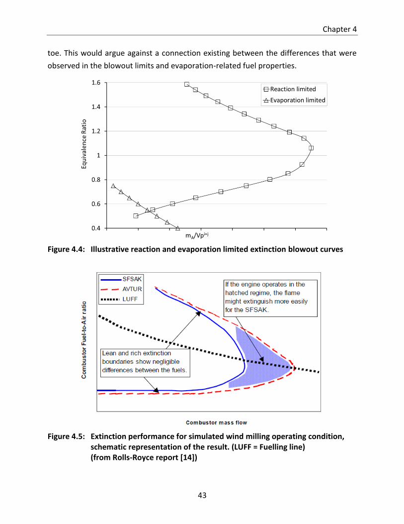
Chapter 4
43
toe. This would argue against a connection existing between the differences that were
observed in the blowout limits and evaporation-related fuel properties.
Figure 4.4: Illustrative reaction and evaporation limited extinction blowout curves
Figure 4.5: Extinction performance for simulated wind milling operating condition,
schematic representation of the result. (LUFF = Fuelling line) (from Rolls-Royce report [14])

Theoretical Assessment
44
4.4 Combustion Efficiencies
Evaporation-, mixing-, and reaction-controlled efficiencies can also be considered in
terms of fluid-mechanic and chemical timescales to gain insight into their relevance
under the different combustor conditions and how they potentially impact combustion
limits. The usefulness of representing combustion efficiency in this way will be seen
later in Chapter 7.
4.4.1 Evaporation-controlled efficiency
Equation 2.6 was used to express the evaporation-controlled combustion efficiency in
terms of the combustor operating conditions (𝜌𝐴 , 𝜆𝑒𝑓𝑓 , �̇�𝐴), physical combustor
dimensions (V), fuel spray characteristics (D0) and fuel properties (D0 , 𝜆𝑒𝑓𝑓).
Rearranging Equation 2.6, the evaporation-controlled combustion efficiency can be
expressed as Equation 4.27.
𝜂𝑒 ∝ (𝜌𝐴𝑉
�̇�𝐴) (
𝜆𝑒𝑓𝑓
𝐷02 ) [4.27]
The first term on the right hand side of the equation is equivalent to the residence time
of the air in the combustion chamber, 𝜏𝑟𝑒𝑠 and, as discussed in Appendix A, the second
term is the inverse of the droplet lifetime or evaporation delay time, 𝜏𝑒. The expression
therefore represents the logical argument that the combustion efficiency amounts to
the ratio of the air residence time in the combustor to the droplet evaporation time.
𝜂𝑒 =𝐴𝑖𝑟 𝑟𝑒𝑠𝑖𝑑𝑒𝑛𝑐𝑒 𝑡𝑖𝑚𝑒
𝐷𝑟𝑜𝑝𝑙𝑒𝑡 𝑒𝑣𝑎𝑝𝑜𝑟𝑎𝑡𝑖𝑜𝑛 𝑡𝑖𝑚𝑒=
𝜏𝑟𝑒𝑠
𝜏𝑒 [4.28]
It is possible to illustrate the blowout limit of a given fuel (and at a chosen combustion
efficiency limit) by expressing both the air residence time and evaporation time in terms
of air mass flow rate. In a laboratory model-combustor operated at constant pressure
and temperature, the fluid-mechanic timescale, or air residence time, becomes a
function of the inverse of the air mass flow rate. Recalling Equation 2.28 for SMDs and
assuming constant hardware dimensions, fuel properties, the relative velocity and
associated effective evaporation constant of finely atomised droplets being relatively
insensitive to the air mass flow rate [20, 56], and with 1 +1
𝐴𝐿𝑅≈ 1 the droplet
evaporation can be approximated as:
𝜏𝑒 = (𝐷02
𝜆𝑒𝑓𝑓) ∝ (
1
𝑚𝐴̇2) [4.29]

Chapter 4
45
Figure 4.6: Illustrative timescales in an evaporation limited system with fixed inlet
pressure and temperature
Figure 4.6 represents an evaporation-controlled system where the limiting combustion
efficiency has been assumed to be at 80%. Combustion can be sustained as long as the
residence time is greater than 80% of the evaporation delay. This would dictate a
minimum air mass flow rate at which blowout occurs and below which combustion is
impossible. At any airflow rates above the blowout point the air residence time would
be sufficient for the evaporation efficiency to be greater than 80% and evaporation
would not play a limiting role. This confirms the conclusion from Section 4.3 and
Figure 4.4 that evaporation limits are expected to constrain combustion at lower air
mass flow rates. Fuel-related differences in properties that effect evaporation would be
relevant under these conditions, but play a much less important role at higher mass flow
rates.
4.4.2 Mixing-controlled efficiency
The combustion efficiency in a mixing-controlled system was expressed by
Equation 2.11.
𝜂𝑚 = 𝑓 ((𝑃3𝐴𝑟𝑒𝑓 �̇�𝐴𝑇30.5⁄ )(∆𝑃𝐿 𝑃3⁄ )0.5) [2.11]

Theoretical Assessment
46
∴ 𝜂𝑚 ∝ (𝜌𝐴𝑟𝑒𝑓
�̇�𝐴) (
𝑇3∆𝑃𝐿
𝑃3)0.5
[4.30]
∴ 𝜂𝑚 ∝ (𝜌
�̇�𝐴) (
𝑇3(𝜌𝑣2)
𝑃3)0.5
[4.31]
∴ 𝜂𝑚 ∝ (𝜌𝐴𝑟𝑒𝑓𝑣
�̇�𝐴) [4.32]
Assuming a fixed dimensionless ratio to exist between the area of the liner air holes and
the combustor reference area (Aref), the numerator is also equal to the air mass flow
rate. This indicates that both 𝜏𝑟𝑒𝑠 and 𝜏𝑚𝑖𝑥 are proportional to 1/�̇�𝐴.
Figure 4.7: Illustrative timescales in a mixing limited system with fixed inlet pressure
and temperature
For any given pressure and temperature condition, the efficiency is nominally
independent of air mass flow rate and is essentially dependent only on the ratio of the
area of the liner air holes to the combustor cross-section area.
4.4.3 Reaction-controlled efficiency
Rearranging Equation 2.31 for reaction-controlled combustion efficiency yields
Equation 4.27.
𝜂𝜃 ∝ 𝑉𝑒−𝐸 𝑅𝑇⁄ 𝜌1.75 �̇�𝐴⁄ [2.31]

Chapter 4
47
∴ 𝜂𝜃 ∝ (𝜌𝑉
�̇�𝐴) (𝑒−𝐸 𝑅𝑇⁄ 𝑃0.75) [4.27]
The first term on the right hand side of the equation is again equivalent to the residence
time, 𝜏𝑟𝑒𝑠 , while the second term is the inverse of a common expression for the
reaction induction time or so-called ignition delay time, 𝜏𝜃 [57]. The combustion
efficiency is therefore in fact simply being expressed as the air residence time divided by
the combustion induction time which is equivalent to the Damköhler number, Da:
𝜂𝜃 =𝐴𝑖𝑟 𝑟𝑒𝑠𝑖𝑑𝑒𝑛𝑐𝑒 𝑡𝑖𝑚𝑒
𝐶𝑜𝑚𝑏𝑢𝑠𝑡𝑖𝑜𝑛 𝑖𝑛𝑑𝑢𝑐𝑡𝑖𝑜𝑛 𝑡𝑖𝑚𝑒=
𝜏𝑟𝑒𝑠
𝜏𝜃 ≡ 𝐷𝑎 [4.28]
In a laboratory model-combustor operating at constant pressure and temperature the
fluid-mechanic timescale or air residence time becomes a function of the inverse of the
air mass flow rate while the chemical timescale will be constant. Figure 4.8 represents
this diagrammatically for a system where the limiting combustion efficiency has again
been assumed to be at 80%. Combustion can be sustained as long as the residence time
is greater than 80% of the ignition delay which dictates a maximum air mass flow rate at
which blowout occurs and beyond which combustion is impossible.
Figure 4.8: Illustrative timescales in a chemical reaction limited system with fixed inlet
pressure and temperature.

Theoretical Assessment
48
The diagrams presented in this section were chosen to illustrate the relative timescale
behaviour in a combustor having fixed inlet pressure and temperature. Obviously one
could consider the relative timescale behaviour under other scenarios such as fixed air
mass flow and varying inlet pressure or temperature. However, it was the principle of
viewing the efficiency as the ratio of two competing timescales that is useful in this
present work.
The subsequent chapter details the experimental approach that was designed to
interrogate the thesis hypotheses by examining how the theoretical evaporation- and
reaction-controlled combustion efficiencies translate to practical combustion behaviour.

49
5 Experimental Design
An experimental programme was designed based on the insights gained from the
theoretical treatment and literature review to provide data to explore how fuel
properties can impact combustion efficiency and extinction under representative gas
turbine combustion conditions. The programme was also intended to provide data for
answering the hypotheses and explaining the LBO differences that were observed
during the fully synthetic jet fuel (FSJF) certification tests. It consisted of the following
main components:
Design of a test fuel matrix
Physical and chemical characterisation the fuel matrix
Evaluation of the test fuel LBO behaviour in a laboratory-scale model-combustor
Evaluation of the test fuel spray behaviour in a laboratory-scale model-combustor
5.1 Test fuel matrix
The theoretical assessment implicitly proposed a research strategy for revealing the root
cause if it were possible to evaluate a number of fuels that exhibit independently varied
properties relating to evaporation and reaction behaviour. It is, however, virtually
impossible to change fuel properties entirely orthogonally which complicates the
selection of appropriate test fuels and the interpretation of test results. The design of
the test fuel matrix was influenced by a combination of the desire to include fuels that
were representative of those employed during the FSJF certification process and results
from previous laboratory-scale extinction and ignition work [7, 58] which included both
full boiling range and single component test fuels. The primary goal was to investigate
the relative influence of fuel properties on evaporation rate and reaction rate
independently in a combustion environment. It was therefore important to differentiate
key properties to as large a degree as possible, while still employing fuels that
resembled current commercial jet fuels. The resultant matrix entailed a selection of
eight fuels that were nominally representative of either crude-derived or viable
alternative jet fuel formulations. It included fuels that complied fully with the Jet A-1
specification such as crude-derived and Fischer–Tropsch (FT) derived synthetic
commercial fuels as well as fuels that were formulated to intentionally breach the
specification on selected properties that were of interest. Table 5.1 reflects the test fuel

Experimental design
50
matrix with a selection of crude-derived Jet A-1, synthetic paraffinic kerosene, linear
paraffinic solvents, aromatic solvents and pure compounds. While the matrix included
some synthetic jet fuel formulations, the primary focus was on fuel properties
regardless of the production pathways employed to produce the fuels.
Table 5.1: Test fuel matrix
CJF Crude-derived Jet A-1
CJF/D Jet A-1 + 50% n-dodecane
SJF1 FSJF (certification)
SJF2 FSJF (commercial)
SJF2+ FSJF (commercial) + 1.5% HCPP
LTSK Experimental GTL kerosene
HTSK Synthetic paraffinic kerosene (SPK)
HN Heavy naphtha refinery stream
CJF was a commercial crude-derived Jet A-1 while CJF/D was a 50:50 blend of CJF and n-
dodecane. SJF1 was formulated to be representative of the FSJF that was used during
the 2006 certification process and the associated test program, while SJF2 was
representative of a FSJF formulation that would comply with the distillation gradient
specification that was introduced for FSJF as part of DEFSTAN 91-91 [59] in 2008. SJF2+
was a blend of 98.5% SJF2 and 1.5% hydrogenated cat-poly petrol (HCPP) which was
added to investigate the influence of flash point. HTSK was a Synthetic paraffinic
kerosene stream that is typically employed in both fully and semi-synthetic jet fuel. HN
was a heavy naphtha refinery stream and LTSK a gas-to-liquids (GTL) kerosene that were
both included to assist in evaluating non-orthogonal changes in the various fuel
properties. LTSK was of further interest due to the fact that it nominally resembled a
fuel that could also be produced via a renewable synthetic jet fuel manufacturing
process. The influence of the LTSK’s largely linear paraffin structure on ignition delay,
cetane, and LBO was also of interest in light of the observations that have been
highlighted by literature as discussed in Chapter 3 [8, 10, 11].

Chapter 5
51
5.2 Physical characterisation of test fuel matrix
The test fuel matrix was characterised employing the standard test methods employed
in the aviation industry as specified by ASTM D1655 [60]. While full-specification
analyses were performed, the physical properties that were of primary interest included
density, viscosity, flash point, and the distillation profiles. Concerns have been raised
within the aviation industry regarding the sensitivity of the D86 method that is
stipulated by ASTM D1655 for determining distillation profiles. Therefore, apart from
the conventional D86 method, a GC-based simulated distillation was also conducted
according to ASTM D2887 [61]. Surface tension measurements were performed at 25°C
and 40°C, and refractive indices were determined to be employed by the Phase Doppler
Anemometry (PDA) measurements during the fuel spray characterisation.
5.3 Chemical characterisation of test fuel matrix
In addition to the normal (physical) jet fuel specification tests a number of
measurements were conducted to characterise the chemical composition and reactivity
of the test fuels. Comprehensive two–dimensional gas chromatography (GCxGC), where
two independent separations are applied to a single sample injection, is considered to
be the most accurate means to obtain detailed compositional information for complex
petrochemical mixtures. This technique offers structured separations, high sensitivity
and high peak capacity. Complex fuels are traditionally analysed in the so-called
“normal” GCxGC mode where a non–polar column is used in the first dimension to
perform a boiling-point based separation. A thermal modulator is used to focus the
effluent from the first column onto a polar column which provides separation in the
second dimension based on polarity. For this study the analyses were performed in the
so-called “inverse mode” where the first dimension employs a polar column and the
second dimension employs a non–polar column. This sequence is considered to be less
orthogonal but has been demonstrated to extend the separation space when used to
characterise FT fuels and the aromatic fractions in petroleum middle–distillates resulting
in improved resolution [62]. Chemical structures were elucidated by time–of–flight mass
spectrometry (TOF–MS), and a flame ionisation detector (FID) was used for
quantification. The two-dimensional gas chromatography results provided information
about the test fuel chemical compositions and were used to determine carbon to

Experimental design
52
hydrogen ratios that were required to calculate the stoichiometric fuel/air ratio (FAR)
for each test fuel.
Tests were also conducted to characterise the chemical reactivity of the fuels. An IQT™
combustion bomb (manufactured by AET, Canada) was employed to determine ignition
delay times of the test fuel matrix. This automated test method is used for the
quantitative determination of the ignition characteristics of specifically middle-distillate
fuels and fuel blending components. The IQT™ utilises a constant-volume combustion
chamber that is pre-heated electrically to 843 K. Test fuel is injected directly into the
chamber filled with synthetic air at 2.1 MPa. An empirical calibration formula, as
specified in ASTM D 6890 [63], is used to convert the measured ignition delay to a
derived cetane number. This is a combustion quality indicator used primarily in diesel
engine applications.
Laminar flame speed (LFS) has been suggested as a combustion indicator that could
potentially be appropriate for evaluating gas-turbine performance [42, 43, 64]. A
pressure-based method making use of a spherical bomb was employed to measure the
LFS and Markstein length of the test fuels. Tests were conducted at ambient initial
pressure and two initial temperatures with six different air-fuel ratios spanning the
range from lean to rich. A minimum of six repeat combustion pressure records of
approximately 90 data points were obtained for each test fuel which yielded a database
of over 6000 individual calculations of LFS from which the relevant parameter
coefficients could be calculated using a regression technique. The experimental
hardware and analysis methodology are described in greater detail by Yates et al. [64].
Peak LFS values were calculated at an equivalence ratio of ɸ = 1.075 and reference
conditions of 298.15 K and 101.325 kPa.
Ignition delays were determined by the Institute of Combustion Technology at the
German Aerospace Centre (DLR) in Stuttgart, Germany. A high pressure shock tube was
employed with an internal diameter of 98.2 mm. The 5.18 m long driver section and
11.12 m long driven section were separated by aluminium diaphragms. A turbo-
molecular pump was used to evacuate the driven section to pressures below 10-6 mbar.
Gas mixtures were prepared manometrically in an evacuated stainless steel storage
cylinder at pressures below 10-6 mbar. Four piezo-electric pressure sensors at 20 cm
intervals were used to calculate the incident shock speed. A one-dimensional shock
model was used to calculate the temperature and pressure behind the reflected shock

Chapter 5
53
wave from the measured incident shock speed and the speed attenuation. The resultant
uncertainty in the calculated reflected shock temperature was less than 10 K. Piezo-
electric pressure sensors (PCB® 113A24 and Kistler® 603B) located 1 cm from the end
flange, were used to observe the pressure profiles associated with ignition.
OH*-emission (at 308 nm) and CH*-emission (at 431 nm) were measured using a
photomultiplier and narrow band filter (full width at half maximum - FWHM of 5 nm).
The ignition delay time values were calculated as the time elapsed between the system
being initiated by the reflected shock wave and the maximum OH*-emission being
recorded. Ignition delay times of up to 6.5 ms can be measured by the experimental
setup depending on the temperature. All tests were performed at initial pressures of
1.6 MPa ± 10% with synthetic air (20%v O2 in N2). Reaction mixtures were diluted 1:2,
i.e. one part undiluted mixture and one part N2.
5.4 Gas turbine model-combustor: LBO evaluation
The LBO behaviour of the eight test fuels were evaluated using a laboratory-scale
model-combustor at the German Aerospace Centre (DLR). The combustor was based on
previous spray burner research [65] and was designed to be representative of the
primary zone encountered in real aero-engines. The scaling of the combustor was a
compromise to accommodate practical laboratory constraints while retaining technical
relevance. The resultant rig was designed for thermal powers of approximately 10 kW at
atmospheric pressure conditions.
The core of the combustor consisted of the burner nozzle shown in Figure 5.1. A
common air plenum supplied air to inner and outer air swirlers that produced two co-
axial, co-rotating swirl flows that were separated by a thin annular ring with a sharp
edge. A pressure-swirl atomiser produced a hollow cone of fuel spray through two swirl
channels that was sprayed onto the inside of the annular ring. A fuel film formed on the
surface and was transported to the lip of the ring where it re-atomised. This so-called
prefilming airblast atomisation concept is widely used in current combustion
systems [66].

Experimental design
54
Figure 5.1: Laboratory-scale model burner nozzle (configuration B) [65]
The combustion chamber consisted of four quartz windows that were held in place by
steel posts. The resultant optical access allowed the application of a host of optical and
laser-based diagnostic techniques. A top plate secured the windows and posts. The
19 mm diameter exit port in the top plate exhausted to atmospheric pressure. The
chamber had a cross section of 85 mm by 85 mm and a length of 169 mm which was
sufficient to fully contain combustion throughout the operating conditions that were
investigated. Specific care was taken to ensure cylindrical symmetry of the spray cone
and resultant combustion zone.
The experimental layout of the model-combustor is shown in Figure 5.2. A mass flow
controller (Bronkhorst EL-FLOWselect F-203AV) was used to regulate supply of dry
compressed air to the air plenum. The air temperature was controlled by an electric pre-
heater based on the temperature inside the air plenum measured using a K-type
thermocouple. A sonic nozzle decoupled the combustor acoustically from the air feed
line while meshes were used to homogenise the air flow into the plenum. The test fuel
was supplied from a piston driven stainless steel cylinder which ensured that the
nitrogen driver gas was not in contact with the test fuel. The test fuel was also degassed
prior to testing by applying a mild vacuum to the supply cylinder. A mass flow controller
(Bronkhorst mini CORI-FLOW M14) regulated the fuel supply to the fuel pressure
atomiser via a water-cooled fuel lance. The fuel temperature control was based on the
temperature measured just upstream of the atomiser exit. The development of the test
apparatus is discussed in greater detail by Grohmann et al. [65].

Chapter 5
55
Two burner configurations (A and B) were tested with different swirl numbers. The swirl
number is defined as the ratio of the angular momentum flux, 𝐺𝜃, divided by the axial
momentum flux, 𝐺𝑦, and a characteristic radial distance, R [67, 68].
𝑆 = 𝐺𝜃
𝐺𝑦𝑅 [5.1]
Subsequent to the completion of the LBO tests with burner configuration A,
stereoscopic particle image velocimetry (PIV) measurements were conducted of the
non-reacting and reacting flows during an unrelated test program at DLR. The PIV results
revealed the absence of a strong central recirculation zone as would be present in
typical real aero-engine combustors. This was ascribed to lower geometric swirl with a
centre swirl number of Sc = 0.6. The burner was modified, and the resultant second
configuration (B) exhibited a well-developed central recirculation zone with a
geometrical swirl number of Sc = 1.17 for the centre flow and Sa = 1.22 for the annular
flow.
Figure 5.2: Laboratory-scale model-combustor layout [65]
The LBO tests of configuration A were conducted at two air pre-heat temperatures,
323 K and 413 K, while the tests of configuration B were only conducted at 323 K due to
the limited volume of test fuel available. The fuel temperature was controlled to 303 K

Experimental design
56
for the low air pre-heat tests and to 323 K for the high air pre-heat tests. For each air
pre-heat condition, a series of tests were conducted over range of air flow rates ranging
from 2.2 g/s to 12.9 g/s. The air mass flow rate was kept constant for each test point
operating condition. Combustion was established at a stoichiometry of approximately
ɸ = 0.7, well within the stable combustion operating envelope, following which the fuel
mass flow rate was reduced at a controlled rate of 0.5 (g/h)/s up to the point of
blowout. This corresponded with a ɸ reduction rate of 0.001 s-1 to 0.0001 s-1 depending
on the air mass flow rate. The stoichiometry and air mass flow rate at the point of
extinction was recorded as the LBO point. A minimum of three repeat tests were
conducted at each operating condition. The model-combustor set-up and a
stoichiometric Jet A-1 reference flame are shown in Figures 5.3 and 5.4 respectively.
Figure 5.3: Model-combustor setup Figure 5.4: Reference Jet A-1 flame (ɸ = 1, Tair = 323 K)
5.5 Gas turbine model-combustor: fuel spray evaluation
A three component Phase Doppler Anemometry (PDA) system by Artium Technologies
Inc. (PDI-300 MD) was used to investigate the fuel spray in the model-combustor. The
droplet diameters as well as radial, axial and circumferential velocity components of the

Chapter 5
57
droplets were measured during combustion close to LBO. Three pairs of laser beams
were generated by three diode pumped solid state lasers contained in the two
transmitting units: 532 nm for axial velocity and diameter measurements, and 491 nm
and 561 nm both for radial and circumferential velocity measurements. Negative
velocity measurements were enabled by frequency shifting one beam of each of the
beam pairs using a Bragg cell. The receiving unit collected the signal in a 45° forward
scatter configuration. The focal length of the optics was 350 mm with the beam waist in
the measurement volume of between 150 and 180 µm depending on the 3 wavelengths.
Droplet measurements of between 0.7um and 100um were attainable with the spatial
aperture of 500um that was applied. The characterisation of smaller droplets was
optimised by adjusting the amplifier voltages of the signal receiving photo multipliers
based on local measurement requirements which minimised saturation of the photo
multipliers while still maximising small droplet signal. A refractometer was used to
determine the refractive indices of the eight test fuels at room temperature.
Measurements were conducted at two stoichiometric air-fuel ratios: one at the LBO
stoichiometry plus 5% and another at a stoichiometry of ɸ = 0.6. This allowed both
investigation of the spray behaviour as close to blowout as practical, as well as a
comparison between all fuels at exactly the same stoichiometric air-fuel ratio. For each
stoichiometric set point, measurements were performed at two air flow rates: 2.2 g/s
and 6.5 g/s which allowed evaluation both below and above the flow rate range where a
distinct air flow-related influence was detected in the LBO behaviour as discussed in the
following chapter.
The combustor was mounted on a three-axis traversing stage that was driven by stepper
motors. This allowed the positioning of the measurement volume within the
combustion zone. The coordinate system is shown in Figure 5.2. Measurements were
performed at three distances from the nozzle exit plane: z = 15 mm, z = 25 mm, and
z= 35 mm. At each z-axis location the combustor was traversed along the y-axis in 2 mm
increments. A minimum of 2500 droplet measurements, that were coincident for all
three channels, were recorded at each measurement point. This resulted in diameter
values being based on between 3000 and 135000 readings per position depending on
the position and operating conditions.
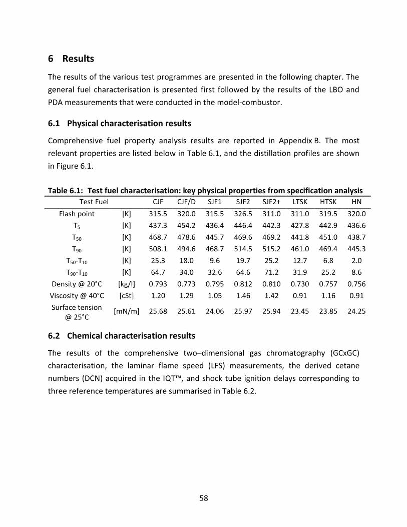
58
6 Results
The results of the various test programmes are presented in the following chapter. The
general fuel characterisation is presented first followed by the results of the LBO and
PDA measurements that were conducted in the model-combustor.
6.1 Physical characterisation results
Comprehensive fuel property analysis results are reported in Appendix B. The most
relevant properties are listed below in Table 6.1, and the distillation profiles are shown
in Figure 6.1.
Table 6.1: Test fuel characterisation: key physical properties from specification analysis
Test Fuel CJF CJF/D SJF1 SJF2 SJF2+ LTSK HTSK HN
Flash point [K] 315.5 320.0 315.5 326.5 311.0 311.0 319.5 320.0
T5 [K] 437.3 454.2 436.4 446.4 442.3 427.8 442.9 436.6
T50 [K] 468.7 478.6 445.7 469.6 469.2 441.8 451.0 438.7
T90 [K] 508.1 494.6 468.7 514.5 515.2 461.0 469.4 445.3
T50-T10 [K] 25.3 18.0 9.6 19.7 25.2 12.7 6.8 2.0
T90-T10 [K] 64.7 34.0 32.6 64.6 71.2 31.9 25.2 8.6
Density @ 20°C [kg/l] 0.793 0.773 0.795 0.812 0.810 0.730 0.757 0.756
Viscosity @ 40°C [cSt] 1.20 1.29 1.05 1.46 1.42 0.91 1.16 0.91
Surface tension @ 25°C
[mN/m] 25.68 25.61 24.06 25.97 25.94 23.45 23.85 24.25
6.2 Chemical characterisation results
The results of the comprehensive two–dimensional gas chromatography (GCxGC)
characterisation, the laminar flame speed (LFS) measurements, the derived cetane
numbers (DCN) acquired in the IQT™, and shock tube ignition delays corresponding to
three reference temperatures are summarised in Table 6.2.

Chapter 6
59
Figure 6.1: Test fuel volatility: distillation profiles.
Table 6.2: Test fuel characterisation: GCxGC speciation, DCN, LFS and shock tube ignition delays
Test Fuel CJF CJF/D SJF1 SJF2 SJF2+ LTSK HTSK HN
normal-paraffins [wgt%] 24.0 60.3 8.2 2.5 2.4 67.9 0 38.1
iso-paraffins [wgt%] 28.3 14.9 65.1 43.6 44.5 31.1 92.0 34.7
cyclic paraffins [wgt%] 20.4 10.6 9.1 14.4 14.3 1.0 7.6 17.6
bicyclic paraffins [wgt%] 4.6 2.3 2.8 20.8 20.4 0 0 1.6
tricyclic paraffins [wgt%] 0.3 0 0 7.5 7.4 0 0 0
alkyl benzenes [wgt%] 15.7 8.2 12.8 2.9 2.9 0 0 7.6
cyclic alkyl benzenes [wgt%] 4.4 2.3 1.8 8.0 7.8 0 0 0.4
naphthalenes [wgt%] 2.3 1.2 0 0.3 0.3 0 0 0
C/H ratio 1.93 2.04 2.02 1.95 1.95 2.20 2.16 2.09
LFS [m.s-1] 0.358 0.353 0.345 0.351 0.350 0.338 0.345 0.352
IDIQT [ms] 4.50 3.45 6.68 7.06 7.14 3.24 7.14 3.88
DCN 45.9 58.5 32.4 30.9 30.6 62.0 30.6 52.6
ID1250 K (1000/T = 0.8) [ms] 0.29 0.31 0.34 0.26 0.26 0.22 0.32 0.24
ID1000 K (1000/T = 1.0) [ms] 2.52 2.61 3.05 2.34 2.31 1.94 2.92 2.07
ID833 K (1000/T = 1.2) [ms] 13.25 9.08 22.90 17.07 15.09 10.08 21.11 9.94

Results
60
The IQT™-measured ignition delays (IDIQT) were converted to DCN values using the
empirical calibration described by Equation 6.1 [69].
𝐷𝐶𝑁 = 83.99 (𝐼𝐷𝐼𝑄𝑇 − 1.512)−0.658
+ 3.547 [6.1]
The constant 1.512 ms offset that was applied to all the measured ignition delays
accounted for the evaporation and mixing delays that are intrinsic to the heterogeneous
injection in the IQT™ bomb.
While the physical characterisation, compositional analyses, laminar flame speed, and
IQT™ ignition delay results could be used without significant processing, the data from
the shock tube ignition delay experiments had to be analysed further. The data points
spanned both the high-temperature and low-temperature regimes with a number but
not all of the fuels recording delays into the negative temperature coefficient (NTC)
region. Yates et al [70] proposed a convenient method of describing the ignition delays
in each of the distinct temperature regimes using generic Arrhenius functions having the
form:
𝜏𝑖 = 𝐴𝑖𝑝𝑛𝑖𝑒
𝐵𝑖𝑇 [6.2]
Where 𝜏𝑖 represents the ignition delay, A, n and B, are constants and p and T are the
pressure and temperature respectively. They treated the two sequential stages in the
low-temperature regime (low temperature and NTC) as the arithmetic sum of the
individual delays, 𝜏1 + 𝜏2. The high temperature delay, 𝜏3, represented an alternative
competing pathway and the overall ignition delay for both low and high-temperature
was expressed by Equation 6.3.
𝜏𝑜𝑣𝑒𝑟𝑎𝑙𝑙 = ((𝜏1 + 𝜏2)−1 + (𝜏3)
−1)−1 [6.3]
This approach was applied to the shock tube results to smooth over the experimental
noise and intrinsic test-to-test variation in measurement conditions in order to facilitate
direct comparisons between the various fuels. It also facilitated the inclusion of the
ignition delay results in correlation analysis of the fuel properties and LBO test results.
The values of the coefficients A and B for each of the stages were determined by means
of a regression analysis. The pressure dependence was ignored (𝑛𝑖 = 0) due to all tests
being conducted at a common pressure. The shock tube data set did not contain results
that extended into the linear portion of the low-temperature region for all the test fuels,
which essentially reduced the three-Arrhenius to a two-Arrhenius treatment without

Chapter 6
61
influencing the model fit or accuracy in the NTC or high-temperature regions. An
example of the measured results and modelled ignition delay for one of the fuels (test
fuel CJF) is presented in Figure 6.2. The results, modelled ignition delay curves, and
model coefficients for the full fuel matrix are presented in Appendix C. The modelled
ignition delay results for the full matrix are presented in Figure 6.3 while values
calculated for each fuel at 833 K, 1000 k and 1250 K (corresponding with 1000/T values
of 1.2, 1.0 and 0.8 respectively) are included in Table 6.2.
Figure 6.2: Test fuel CJF: Shock tube measured (markers) and modelled (curve)
ignition delay results based on eq. 6.3.

Results
62
Figure 6.3: Modelled ignition delay results for the full tests fuel matrix
The differences in the absolute values of the ignition delays measured in the
homogeneous shock tube and heterogeneous IQT™ are a manifestation of the inherent
differences in operating conditions. It can, however, be expected that fuels with similar
evaporative behaviour exhibit a correlation between IQT™ and shock tube ignition
delays under similar pressure and temperature conditions by virtue of the fuel-to-fuel
differences in the IQT™ ignition delays being reduced primarily to differences in
chemistry. The shock tube measurements in this study were conducted at 16 bar which
did not allow direct comparison with the delays that were measured at 21 bar in the
IQT™ without applying a pressure correction. As mentioned above it was not possible to
calculate an exact pressure correction for each individual fuel due to all the tests being
conducted at the same starting pressure. A reasonable approximation can, however, be
made by applying the pressure dependence of the reaction-controlled combustion
efficiency as expressed in Equation 2.31. The shock tube results also needed to be
adjusted to account for the nitrogen dilution. This was done based on experimental and
modelling work by Zeng et al. [71] which indicated that a correction factor of 0.529 was
applicable. The shock tube ignition delays (ID843 K) were thus converted to IQT™
conditions (ID843 K’) by applying the relationship expressed in Equation 6.4 and are
compared with the IQT™-measured delays in Figure 6.4.

Chapter 6
63
𝐼𝐷843 𝐾′ = 0.529 𝐼𝐷843 𝐾 (
𝑃𝐼𝑄𝑇
𝑃𝑆𝑇)1.75
⁄ [6.4]
where 0.529 is the dilution correction factor [71]. It is interesting to note that the
constant evaporation and mixing delay offset contained in the calculation of DCN values
(Equation 6.1), was also revealed as a constant offset in the best-fit linear trend line in
the comparison with the shock tube ignition delays.
Figure 6.4: Comparison of IQT™ and shock tube ignition delays
The various ignition delay measurements were compared using a correlation matrix
analysis (see Table 6.3) which confirmed that the shock tube ignition delays at 833 K
correlated very strongly with the delays converted to IQT™ conditions (ID843 K‘).
(Absolute coefficients greater than 0.7 were considered indicative of strong correlations
while 0.5 to 0.7 were considered to be indicative of weak but significant correlations.)
The analysis also revealed a strong positive correlation between IQT™ delays and the
shock tube results at 833 K (1000/K = 1.2), but weak correlations in the high
temperature regime, 1000/K = 1.0 and 0.8. While this is not an unqualified result it
confirmed confidence in the ignition delay data sets measured in both the shock tube
and IQT™. Due to the very strong positive correlation revealed between the 1000 K and
1250 K shock tube delays which indicated that these results were essentially covariant,
only the 1000 K metric was used in the subsequent analyses. Similarly the 833 K shock

Results
64
tube delays were subsequently considered to also be a reasonable proxy representation
of results converted to the IQT™ temperature and pressure operating conditions
Table 6.3: Correlation analysis of IQT™ and shock tube ignition delay results
ID1250 K ID1000 K ID833 K ID843 K‘ IDIQT
ID1250 K (1000/T = 0.8) 1
ID1000 K (1000/T = 1.0) 0.99 1
ID833 K (1000/T = 1.2) 0.66 0.76 1
ID843 K‘ 0.67 0.78 1.00 1
IDIQT 0.40 0.51 0.86 0.85 1
-0.5 to 0.5 -0.7 to -0.5 ; 0.5 to 0.7 <-0.7 ; >0.7
6.3 Gas turbine model-combustor: LBO evaluation results
The results of LBO evaluation in the model-combustor are shown in Figures 6.5 to 6.7. It
reports the global equivalence ratios at which the blowout events were detected as a
function of the air mass flow rate for the three different combinations of burner
configuration and air pre-heat temperature.
While there were marked differences in the characteristic shape-functions associated
with the three different combustor test series, they each exhibited statistically
consistent trends for all eight test fuels. Clear differences were observed between the
eight test fuels and superficially these differences appeared to carry through
consistently over the greater part of the air mass flow range and between different test
series.
However, a transition was observed between the results at the lowest air mass flow
rates and the results at higher air mass flow rates above approximately 5 g/s. This was
broadly in line with the behaviour that was predicted by the theoretical treatment in
Section 4.3 as illustrated by Figure 4.3 which showed combustion limits being
constrained by evaporation below a critical air mass flow rate. These results will be
explored in greater detail in a subsequent discussion section.

Chapter 6
65
Figure 6.5: Model-combustor LBO results - burner configuration A, 323 K air pre-heat
Figure 6.6: Model-combustor LBO results - burner configuration A, 413 K air pre-heat

Results
66
Figure 6.7: Model-combustor LBO results - burner configuration B, 323 K air pre-heat
6.4 Gas turbine model-combustor: fuel spray evaluation results
The PDA spray measurements in the laboratory-scale model-combustor were conducted
at two stoichiometric air-fuel ratios: one at 5% rich of the LBO stoichiometry and
another at a stoichiometry of ɸ = 0.6. This allowed both investigation of the spray
behaviour as close to blowout as practical, as well as a comparison between all fuels at
exactly the same stoichiometric air-fuel ratio. For each stoichiometric set point,
measurements were performed at two air mass flow rates (2.2 g/s and 6.5 g/s) and
three distances from the nozzle exit plane (z = 15 mm, z = 25 mm , and z= 35 mm). The
combustor was traversed along the y-axis at each z-axis location in 2 mm increments.
The PDA test results are summarised in Appendix D, which reports Sauter mean
diameter (SMD), D32, values to capture the diameter distribution for each fuel,
combustion condition, and measurement position as a single representative number.
There were no significant differences in the measured behaviour between the two
stoichiometric conditions. The measurements at 6.5 g/s air mass flow rate revealed
clear fuel-specific trends that applied across all test conditions and measurement
positions. All eight test fuels displayed similar distributions over the measurement area
at the higher flow rate.

Chapter 6
67
The measurements at the lower air mass flow rate (2.2 g/s) displayed greater variability
and considerably larger droplet diameters. The spray distributions were also not
consistent across all eight test fuels, with HN deviating from the distribution displayed
by the rest of the test fuels at the lower flow rate.
Figures 6.8 and 6.9 show representative SMD results for ɸ = 0.6 and an air mass flow
rate of 6.5 g/s at the maximum and minimum axial measurement positions. Figure 6.10
reflects the SMD results for an air mass flow rate of 2.2 g/s at ɸ = 0.6 at a distance of
15 mm from the nozzle exit plane. (Note the increase in the vertical scale for Figure 6.10
relating to the lower air mass flow.)
Figure 6.8: Radial SMD profiles (ɸ = 0.6, �̇�𝑨 = 6.5 g/s, z = 15 mm from exit plane)

Results
68
Figure 6.9: Radial SMD profiles (ɸ = 0.6, �̇�𝑨 = 6.5 g/s, z = 35 mm from exit plane)
Figure 6.10: Radial SMD profiles (ɸ = 0.6, �̇�𝑨 = 2.2 g/s, z = 15 mm from exit plane)

69
7 Analysis and Discussion of Results
In the following discussion the results from the different aspects of the experimental
programme are combined to interrogate the influence of various fuel properties on LBO
behaviour. In contrast with the preceding sections, the spray and evaporation behaviour
of the fuels are discussed first because they are important in the evaluation of the so-
called chemical differences. The physical properties and spray behaviour were evaluated
against the theoretical combustion efficiency in an evaporation-controlled system, while
the chemical differences were examined by testing the assumption that the LBO results
had been driven by a reaction-controlled system.
7.1 Spray and evaporation-controlled system analysis of LBO results
The results of the PDA measurements were used to calculate relative SMD values at
each air mass flow condition and for both stoichiometry conditions with CJF as
references. Radial measurements were averaged for each axial measurement positions
and overall for all axial positions. The lower air mass flow rate condition did not yield
sufficient data at the z = 35 mm position for calculating relative SMD numbers. As can be
seen in Table 7.1 the average z-axis values were credible representations of the
measurements at the individual z-axis positions and there was no significant difference
in the relative SMD results between the two stoichiometry conditions. The subsequent
analyses were therefore performed using the average values for the ɸLBO+5% case as
being representative of the PDA performance at the two air mass flow rates.
The spray behaviour was evaluated by comparing the experimental PDA results with
theoretical evaporation-controlled combustion efficiencies for different fuels. Recalling
Equation 2.6, the relative evaporation-controlled combustion efficiencies for two fuels
can be expressed as Equation 7.1.
𝜂𝑒 = 𝜌𝐴𝜆𝑒𝑓𝑓𝑉
𝐷02𝑓𝑐�̇�𝐴
⁄ [2.6]
∴ 𝜂𝑒2𝜂𝑒1
⁄ =𝜆𝑒𝑓𝑓2
𝜆𝑒𝑓𝑓1⁄
(
1𝐷02
𝐷01⁄
)
2
[7.1]

Summary, Conclusions and Recomendations
70
Table 7.1: PDA spray measurements: Relative SMD values averaged per axial measurement position
ɸ z Air mass flow [g/s]
Test Fuel
CJF CJF/D SJF1 SJF2 SJF2+ LTSK HTSK HN
ɸLBO + 5% 15 2.2 1 0.990 1.042 1.016 0.969 0.998 0.949 1.008
ɸLBO + 5% 25 2.2 1 0.993 1.031 1.004 0.963 1.014 1.006 1.009
ɸLBO + 5% Ave 2.2 1 0.991 1.036 1.010 0.966 1.006 0.978 1.009
ɸLBO + 5% 15 6.5 1 0.987 0.910 1.005 0.971 0.924 0.880 0.929
ɸLBO + 5% 25 6.5 1 0.996 0.883 1.022 0.980 0.915 0.880 0.912
ɸLBO + 5% 35 6.5 1 0.983 0.864 1.021 0.992 0.897 0.866 0.899
ɸLBO + 5% Ave 6.5 1 0.989 0.886 1.016 0.981 0.912 0.875 0.913
0.6 15 2.2 1 0.959 1.006 1.003 0.943 0.973 0.936 0.993
0.6 25 2.2 1 1.001 1.041 1.015 0.975 1.038 1.021 1.024
0.6 Ave 2.2 1 0.980 1.024 1.009 0.959 1.005 0.978 1.008
0.6 15 6.5 1 0.996 0.915 0.997 0.959 0.910 0.885 0.920
0.6 25 6.5 1 0.998 0.885 1.017 0.986 0.911 0.866 0.889
0.6 35 6.5 1 0.995 0.869 1.023 1.000 0.893 0.856 0.903
0.6 Ave 6.5 1 0.996 0.890 1.012 0.982 0.905 0.869 0.904
The effective evaporation constants were calculated using Equation 7.2 which was
derived empirically from plots by Chin and Lefebvre that relate effective evaporation
constants to normal boiling point, droplet size, velocity, pressure and ambient
temperature [20]. They presented effective evaporation constants versus boiling point
(Tbn) for various values of droplet size-velocity products (UD0) at three pressures and
three ambient temperatures.
𝜆𝑒𝑓𝑓 ∝ 𝑃0.124 𝑇1.652
𝑇𝑏𝑛0.501 [7.2]
The 100 kPa plots were employed as representative of the atmospheric pressure
conditions under which the PDA measurements were performed. Unlike the earlier
treatment, fuel-specific volatility differences were taken into account by including the
boiling point, Tbn. The boiling point of each fuel was approximated as the distillation
temperature at which 50% is recovered. Chin and Lefebvre acknowledged that while a
single fuel property cannot fully describe evaporation characteristics of any given fuel,
average boiling point has the benefit of being directly related to vapour pressure and
fuel volatility. The PDA measurements revealed that the products of velocity and droplet
size, UD0, ranged between 150 and 1000 depending on the test conditions and

Chapter 7
71
measurement position. For any given test point, the fuel-to-fuel variation of UD0 was,
however, relatively insignificant, which implied that nominally representative values
could be used with confidence to calculate evaporation constants over the full spectrum
of test conditions. Comparison of different system temperatures revealed that while the
absolute values of the effective evaporation constants were influenced strongly, the
relative numbers were insensitive to system temperature. This enabled the use of
nominally representative values of system temperature with confidence.
The relative SMD values were modelled based on Equation 2.28. By comparing relative
SMD numbers, the influence of velocity and the characteristic dimension were
cancelled. Air/liquid ratios (ALRs) at the relevant stoichiometry conditions (ɸ = 0.6 and
ɸ = ɸLBO+5% respectively) were employed although it should be noted that the relative
results were not significantly impacted.
𝑆𝑀𝐷 ∝ (𝜎
𝜌𝐴𝑈𝐴2𝐷𝑃)0.5
(1 +1
𝐴𝐿𝑅) [2.28]
The results of the modelled relative effective evaporation constants, SMDs, and
evaporation-controlled combustion efficiencies are presented in Table 7.2. Due to the
use of relative normalised metrics the influence of air mass flow was largely eliminated
with only the ALR values introducing differences at the two test conditions. These
differences were, however, of the order of 1% and lower. The relative values were,
therefore, averaged over the test burner configurations, air pre-heat set points, and the
two air mass flow rates at which PDA measurement were performed.
Table 7.2: Average relative effective evaporation constants, SMDs, and evaporation-controlled combustion efficiencies of the test fuel matrix.
Test Fuel CJF CJF/D SJF1 SJF2 SJF2+ LTSK HTSK HN
𝜆𝑒𝑓𝑓.(𝑟𝑒𝑙) 1 0.978 1.064 0.998 0.999 1.078 1.047 1.090
𝑆𝑀𝐷(𝑟𝑒𝑙) 1 0.996 0.970 1.008 1.003 0.953 0.955 0.967
𝜂𝑒(𝑟𝑒𝑙) 1 0.986 1.132 0.982 0.992 1.188 1.147 1.164
An analysis was performed of the linear correlation between these calculated relative
spray and evaporation metrics and the relative experimental PDA results from Table 7.1.
The results of this analysis are presented in Table 7.3 with 𝑆𝑀𝐷(𝑟𝑒𝑙) referring to the
averaged calculated relative SMD values and 𝑃𝐷𝐴(𝑟𝑒𝑙) referring to the measured
relative SMD values. The air mass flow rate conditions (2.2 g/s and 6.5 g/s) are identified
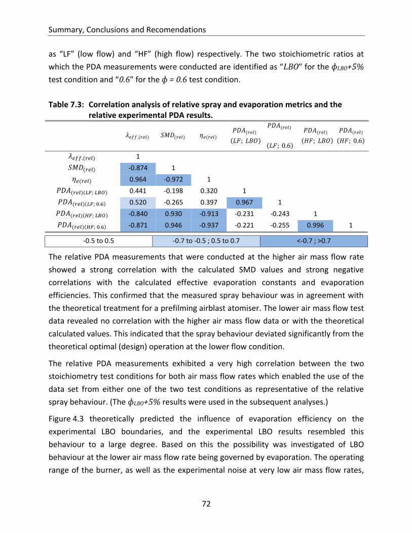
Summary, Conclusions and Recomendations
72
as “LF” (low flow) and “HF” (high flow) respectively. The two stoichiometric ratios at
which the PDA measurements were conducted are identified as “LBO” for the ɸLBO+5%
test condition and “0.6” for the ɸ = 0.6 test condition.
Table 7.3: Correlation analysis of relative spray and evaporation metrics and the relative experimental PDA results.
𝜆𝑒𝑓𝑓.(𝑟𝑒𝑙) 𝑆𝑀𝐷(𝑟𝑒𝑙) 𝜂𝑒(𝑟𝑒𝑙) 𝑃𝐷𝐴(𝑟𝑒𝑙)
(𝐿𝐹; 𝐿𝐵𝑂)
𝑃𝐷𝐴(𝑟𝑒𝑙)
(𝐿𝐹; 0.6)
𝑃𝐷𝐴(𝑟𝑒𝑙)
(𝐻𝐹; 𝐿𝐵𝑂)
𝑃𝐷𝐴(𝑟𝑒𝑙)
(𝐻𝐹; 0.6)
𝜆𝑒𝑓𝑓.(𝑟𝑒𝑙) 1
𝑆𝑀𝐷(𝑟𝑒𝑙) -0.874 1
𝜂𝑒(𝑟𝑒𝑙) 0.964 -0.972 1
𝑃𝐷𝐴(𝑟𝑒𝑙)(𝐿𝐹; 𝐿𝐵𝑂) 0.441 -0.198 0.320 1
𝑃𝐷𝐴(𝑟𝑒𝑙)(𝐿𝐹; 0.6) 0.520 -0.265 0.397 0.967 1
𝑃𝐷𝐴(𝑟𝑒𝑙)(𝐻𝐹; 𝐿𝐵𝑂) -0.840 0.930 -0.913 -0.231 -0.243 1
𝑃𝐷𝐴(𝑟𝑒𝑙)(𝐻𝐹; 0.6) -0.871 0.946 -0.937 -0.221 -0.255 0.996 1
-0.5 to 0.5 -0.7 to -0.5 ; 0.5 to 0.7 <-0.7 ; >0.7
The relative PDA measurements that were conducted at the higher air mass flow rate
showed a strong correlation with the calculated SMD values and strong negative
correlations with the calculated effective evaporation constants and evaporation
efficiencies. This confirmed that the measured spray behaviour was in agreement with
the theoretical treatment for a prefilming airblast atomiser. The lower air mass flow test
data revealed no correlation with the higher air mass flow data or with the theoretical
calculated values. This indicated that the spray behaviour deviated significantly from the
theoretical optimal (design) operation at the lower flow condition.
The relative PDA measurements exhibited a very high correlation between the two
stoichiometry test conditions for both air mass flow rates which enabled the use of the
data set from either one of the two test conditions as representative of the relative
spray behaviour. (The ɸLBO+5% results were used in the subsequent analyses.)
Figure 4.3 theoretically predicted the influence of evaporation efficiency on the
experimental LBO boundaries, and the experimental LBO results resembled this
behaviour to a large degree. Based on this the possibility was investigated of LBO
behaviour at the lower air mass flow rate being governed by evaporation. The operating
range of the burner, as well as the experimental noise at very low air mass flow rates,

Chapter 7
73
resulted in a very limited set of data points in the low flow region that was of interest.
This limited the value that could be gained from comparing LBO trends in this range with
theoretical evaporation efficiencies. An alternative approach was followed by
considering the postulate that the effect of evaporation efficiency resulted in a relative
offset in blowout extinction boundaries and that this would be proportional to the
differences in LBO behaviour in the lowest air mass flow rate while the higher flow
region was shown to be governed by the chemical reaction rate (Figure 4.4). The
magnitude of the “offset” was therefore represented by the numerical difference in
extinction stoichiometries at the lowest air mass flow rate of 2.2 g/s and the 8.6 g/s test
point. The results were then normalised for each test configuration by subtracting the
results of the CJF fuel in that particular configuration. The two low-preheat temperature
test configurations were chosen because they were likely to represent the more
extreme fuel evaporation situation where the fuel differences would be more readily
discerned. It was not considered to be technically defensible to include the higher pre-
heat case. These measured phi “offset” values were compared against theoretical phi
values that were calculated with Equation 7.3 which was derived from equations 2.6, 7.2
and 2.28.
𝜙 ∝ (𝑃0.124 𝑇1.652
𝑇𝑏𝑛0.501𝜂𝑒𝜎
)0.5
− 1 [7.3]
By applying an appropriate proportionality constant the correlation between theoretical
and experimental phi values could be determined. Both burner configurations revealed
positive correlations. Configuration A revealed a weaker and configuration B a stronger
positive correlation. The results from these two burner configurations were, therefore,
combined to reduce the influence of experimental scatter. The fact that a combination
of the two data sets resulted in an improved maximum correlation indicated the benefit
of reducing the influence of experimental noise as reflected by Figure 7.1 graphically.
Figure 7.2 reports the correlation at the optimal combination of the two data sets
comprising of 75% B and 25% A.
Regardless of whether the configurations are viewed individually, numerically averaged,
or the optimal combination of the data sets is used, the correlations supported the
hypothesis that the LBO behaviour at low air mass flow was governed by evaporation
efficiency.

Summary, Conclusions and Recomendations
74
Figure 7.1: Correlation of experimental and theoretical stoichiometric values (effect of proportional representation of configurations A and B)
Figure 7.2: Correlation of experimental and theoretical stoichiometric values (75% configuration B and 25% configuration A)

Chapter 7
75
7.2 Reaction-controlled system analysis of LBO results
The possibility of ignition delay differences influencing the LBO differences that were
recorded in the model-combustor was investigated by recalling the model treatment of
a well-stirred homogeneous reactor (representative of a reaction-controlled system) as
developed in Chapter 4. The relationship between the volumetric flow rate through the
combustor and the combustion efficiency (the extent to which combustion was
completed during the available residence time) are described by Equations 4.18 and
4.23 for lean and rich combustion respectively. These expressions were used to
generate Figures 4.2 and 4.3 to illustrate theoretical differences in LBO behaviour driven
by differences in AFT and proportionality constants which in turn were based on ignition
delay differences.
The model-combustor LBO results were evaluated using the same theoretical treatment
to calculate the best fit values for the proportionality constant of each test fuel. These
constants were subsequently employed in a correlation analysis with fuel properties
(including ignition delay results) and results from the preceding spray behaviour
analysis. Equation 4.18 provided the relevant expression for the relationship between
the volumetric flow rate through the combustor and the combustion efficiency under
the lean conditions that are implicit during LBO.
�̇�𝐴
𝑉𝑃𝑖+𝑗= 𝐾
(1−𝜂𝜃)𝑖𝜙𝑖−1(1−𝜂𝜃𝜙)
𝑗
𝑇𝑖+𝑗𝜂𝜃𝑒−𝐸 𝑅𝑇⁄ [4.18]
The adiabatic flame temperatures at blowout would have been influenced by both the
test fuel composition and stoichiometry. For each test fuel the GCxGC based C/H ratio
was used to calculate the adiabatic flame temperature (AFT) and air fuel stoichiometry
at each LBO point. Heptane-toluene surrogates were used to match the test fuel C/H
ratios as explained previously. A regression analysis of the calculated and measured air
mass flow was then employed to determine the proportionality constant, K, for every
LBO point. The volume was based on the combustor volume, and pressure was
atmospheric, both of which were constant for all fuels. Figure 7.3 represents an example
of these proportionality constants for burner configuration B with air pre-heated to
323 K. The detailed results for all three test configurations are presented in Appendix E.

Summary, Conclusions and Recomendations
76
Figure 7.3: Proportionality constants for modelled combustor airflow based on LBO
test data - burner configuration B, 323 K air pre-heat
The calculated proportionality constants exhibited a flow dependence that would not be
expected in a homogeneous perfectly-stirred reactor. This is indicative of the
homogeneous perfectly-stirred treatment oversimplifying the conditions relevant to the
experimental spray combustor. It was not surprising and could be ascribed to the
additional evaporation, mixing and heat transfer delays that are inherent in the spray
combustor but not applicable in a stirred reactor. These various delay elements would
be influenced by air mass flow rate to different degrees. It was shown in Section 4.4 that
the mixing delay, for example, would be essentially independent of the air mass flow
rate while the evaporation delay would be inversely proportional to the square of the
air mass flow rate. As discussed previously, burner configuration A did not possess a
strong central recirculation zone as would be present in typical real aero-engine
combustors. This was in contrast to configuration B that did exhibit a well-developed
central recirculation zone which resulted in differences in the amount of air and
combustion products being recirculated into their respective primary zones at high flow
rates. Furthermore by increasing air temperature (pre-heat) air viscosity is increased
which influences the entrainment of air into the primary zone. The calculated
proportionality constants of the three burner configuration / pre-heat combinations
would therefore be expected to exhibit different degrees of dependence on air mass

Chapter 7
77
flow rate. This was explored by investigating a modified expression which incorporated
both air mass flow dependent and independent delays.
In the earlier theoretical assessment Equation 4.27 expressed combustion efficiency in
terms of the air residence time and the ignition delay:
𝜂𝜃 = (𝜌𝑉
�̇�𝐴) (𝐾𝑒−𝐸 𝑅𝑇⁄ 𝑃0.75) [4.27]
By rearranging 4.27, the reaction proportionality constant can be expressed as:
𝐾 =𝜌𝑉 �̇�𝐴⁄
𝜂𝜃𝑒−𝐸 𝑅𝑇⁄ 𝑃0.75
[7.4]
A modified proportionality constant which incorporates an additional, fixed delay term
to allow for the physical mixture preparation can then be defined by introducing a
constant delay, 𝜏𝑐, into the air residence time in a manner similar to the treatment of
the IQT™ ignition delay calibration curve (Equation 6.1) discussed in Section 6.2.
𝐾𝜃 =𝜌𝑉 �̇�𝐴⁄ − 𝜏𝑐
𝜂𝜃𝑒−𝐸 𝑅𝑇⁄ 𝑃0.75
[7.5]
∴ 𝐾𝜃
𝐾=𝜌𝑉 �̇�𝐴⁄ − 𝜏𝑐
𝜌𝑉 �̇�𝐴⁄ [7.6]
𝐾𝜃 = 𝐾(1 − 𝐶𝜃�̇�𝐴) where 𝐶𝜃 = 𝜏𝑐
𝜌𝑉 [7.7]
Modified proportionality constants were calculated for each fuel by appropriate
selection of 𝐶𝜃 to minimise the standard deviation in the higher air mass flow region
where the effects of evaporation are diminished, and one could reasonably expect the
modified proportionality constant to be independent of air mass flow rate. The results
for all three configuration / pre-heat combinations are presented in Appendix E. The
modified proportionality constants for burner configurations A and B with 323 K air pre-
heat are shown in Figures 7.4 and 7.5. Configuration A without the strong recirculation
exhibited relatively constant values at air mass flow rates above 6.5 g/s, but
configuration B retained a small measure of flow rate dependence. At the higher pre-
heat temperature, the test results with burner configuration A exhibited even greater
air mass flow dependence. The residual dependence of the modified proportionality
constants on air flow rate could possibly be ascribed to increased entrainment of
secondary air under higher flow turbulence conditions, but importantly does not
significantly impact the relative performance of the different fuels.

Summary, Conclusions and Recomendations
78
Figure 7.4: Modified proportionality constants (Kθ) for modelled combustor airflow
based on LBO test data - burner configuration A, 323 K air pre-heat
Figure 7.5: Modified proportionality constants (Kθ) for modelled combustor airflow
based on LBO test data - burner configuration B, 323 K air pre-heat
The modified and unmodified proportionality constants (as reported in Table E1,
Appendix E) were compared by conducting a correlation analysis of the averaged values

Chapter 7
79
for all three test configurations at flow rates above 8 g/s. Both modified and unmodified
proportionality constants exhibited deviations at air mass flows below 6 g/s which
agreed with the preceding conclusion that evaporation efficiency impacted the blowout
results at low air flow rates. The relative ranking of the fuel constants were similarly
achieved by normalising them to a common reference: Test Fuel CJF. The correlation
analysis results reported in Table 7.4 revealed that the normalised proportionality
constants (K) of the three test configurations correlated strongly with each other and
with their respective modified constants (Kθ). The modified constants of the two low air
pre-heat cases also correlated strongly, but the correlation between the low and high
pre-heat cases were much weaker. The K and Kθ values averaged over their three test
configurations all correlated very strongly the individual configuration rankings with the
exception of the modified constants for the higher pre-heat case of configuration A.
Based on these results the unmodified relative proportionality constants averaged over
all configurations, KAve, were selected for use as the optimal representation of the
chemical reaction rate in subsequent analyses to represent the relative LBO
performance of the fuels.
Table 7.4: Correlation analysis of normalised LBO proportionality constants (K) and modified proportionality constants (Kθ)
K (A , 323 K)
K (B , 323 K)
K (A , 413 K)
KAve
Kθ (A , 323 K)
Kθ (B , 323 K)
Kθ (A , 413 K)
KθAve
K (A , 323 K) 1
K (B , 323 K) 0.892 1
K (A , 413 K) 0.848 0.714 1
KAve 0.976 0.930 0.906 1
Kθ (A , 323 K) 0.712 0.660 0.331 0.614 1
Kθ (B , 323 K) 0.874 0.900 0.521 0.823 0.893 1
Kθ (A , 413 K) 0.873 0.742 0.990 0.922 0.380 0.571 1
KθAve 0.922 0.866 0.647 0.871 0.920 0.963 0.692 1
-0.5 to 0.5 -0.7 to -0.5 ; 0.5 to 0.7 <-0.7 ; >0.7
As a preliminary check on the self-consistency within the various experimental data, the
influence of fuel properties on LBO behaviour was interrogated by analysing the

Summary, Conclusions and Recomendations
80
correlation between the relative LBO proportionality constants (KAve), the relative spray
behaviour (SMD(rel)) and the metrics that were used to define the combustion chemistry
of the fuel matrix (LFS, IDIQT, ID1000 K, ID833 K). The results of the analysis are reported in
Table 7.5. The following conclusions were drawn from the results of this analysis:
The SMD(rel) was chosen to represent the spray behaviour at higher air mass flow
rates because of the very strong correlation with the relative PDA measurements
(as reported in Table 7.3). Under these conditions the spray was fully developed
and adhering to the theoretical treatment for a prefilming airblast atomiser.
There was absolutely no correlation between the LBO proportionality constants
and the relative spray behaviour of the different fuels which confirmed that there
was no discernable influence of evaporation or spray on the blowout results in
the high air mass flow regime.
Table 7.5: Correlation analysis of average relative LBO behaviour, fuel spray, LFS and ignition delays
KAve SMD(rel) LFS IDIQT ID833 K ID1000 K
KAve 1
SMD(rel) 0.07 1
LFS -0.08 0.74 1
IDIQT -0.71 0.22 -0.05 1
ID833 K (1000/T = 1.2) -0.87 -0.11 -0.23 0.86 1
ID1000 K (1000/T = 1.0) -0.84 -0.01 0.07 0.51 0.76 1
-0.5 to 0.5 -0.7 to -0.5 ; 0.5 to 0.7 <-0.7 ; >0.7
Similarly there was absolutely no correlation between the LBO proportionality
constants and LFS which discredited the relevance of LFS being used to predict
the LBO behaviour of different fuels. This provided clarification of the
contradictions in literature regarding the impact of LFS on LBO, that were
identified in Chapter 4.
Relative LBO behaviour, KAve, exhibited a strong inverse correlation with IQT™
ignition delays and even stronger with the two shock tube ignition delays.
However, as was also reported in Table 6.3, while IQT™ delays correlated strongly
with the lower intermediate temperature shock tube ignition delays, the
correlation was weaker with the higher temperature delays. Viewed in
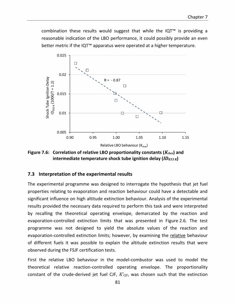
Chapter 7
81
combination these results would suggest that while the IQT™ is providing a
reasonable indication of the LBO performance, it could possibly provide an even
better metric if the IQT™ apparatus were operated at a higher temperature.
Figure 7.6: Correlation of relative LBO proportionality constants (KAve) and
intermediate temperature shock tube ignition delay (ID833 K)
7.3 Interpretation of the experimental results
The experimental programme was designed to interrogate the hypothesis that jet fuel
properties relating to evaporation and reaction behaviour could have a detectable and
significant influence on high altitude extinction behaviour. Analysis of the experimental
results provided the necessary data required to perform this task and were interpreted
by recalling the theoretical operating envelope, demarcated by the reaction and
evaporation-controlled extinction limits that was presented in Figure 2.6. The test
programme was not designed to yield the absolute values of the reaction and
evaporation-controlled extinction limits; however, by examining the relative behaviour
of different fuels it was possible to explain the altitude extinction results that were
observed during the FSJF certification tests.
First the relative LBO behaviour in the model-combustor was used to model the
theoretical relative reaction-controlled operating envelope. The proportionality
constant of the crude-derived jet fuel CJF, K’CJF, was chosen such that the extinction

Summary, Conclusions and Recomendations
82
boundary (based on Equation 2.31) passed through the blowout extinction point that
was recorded by the crude-derived test fuel (AVTUR) during the Rolls-Royce test
campaign: Mach 0.99 at 10760 m (35300 ft.) altitude [13]. The fuel-specific relative LBO
proportionality constants (KAve) that were calculated in the preceding section were
employed in Equation 7.8 to produce the relative extinction limits for the rest of the test
fuel matrix.
𝜂𝜃 ∝ 𝑉𝑒−𝐸 𝑅𝑇⁄ 𝜌1.75 �̇�𝐴⁄ [2.31]
𝜂𝜃 = 𝐾′𝐶𝐽𝐹 𝐾𝐴𝑣𝑒 𝑉 𝑒−𝐸 𝑅𝑇⁄ 𝜌1.75 �̇�𝐴⁄ [7.8]
The results are shown graphically in Figure 7.7 resulting in a number of observations
that can be made. As mentioned, test fuel SJF1 was nominally identical to the synthetic
test fuel that was employed in the FSJF certification tests (SFSAK). A blowout extinction
limit of approximately Mach 0.95 at 10270 m (33700 ft.) altitude was reported for the
SFSAK fuel [13]. The modelled extinction behaviour of SJF1 confirmed this impaired
extinction limit relative to the crude-derived reference CJF/ AVTUR with its extinction
boundary passing through Mach 0.95 at an altitude of 10150 m. (The AVTUR and SFSAK
blowout extinction points are included in figures 7.7 to 7.9 to contextualise the results.)
It is interesting to note that the relative proportionality constants for SJF1 represented a
9 to 12 % reduction in air mass flow at blowout which compares well with the
observation from the altitude test report which stated an almost 6% difference in
relative air flow at first sector blowout and more than 10% difference in final sector
blowout.
The modelled performance of the production synthetic jet fuel formulation, SJF2, was
marginally better than the reference CJF while the low-temperature FT kerosene, LTSK
achieved the highest extinction boundaries.

Chapter 7
83
Figure 7.7: Theoretical relative reaction-controlled extinction limits
Similarly a theoretical relative evaporation-controlled operating envelope was modelled
based on relative spray behaviour and relative effective evaporation constants, again
using CJF as the reference. Incorporating SMD(rel) and the effective evaporation
constants from Equation 7.2 into Equation 2.6 yields Equation 7.9 which was used to
model the relative evaporation-controlled extinction limits. The proportionality constant
K”CJF was again chosen such that the extinction boundary of CJF passed through the
blowout extinction point that was recorded by the AVTUR fuel during the Rolls-Royce
test campaign: Mach 0.99 at 10760 m (35300 ft.) altitude. The resultant extinction
boundaries for all eight test fuels are reported in Figure 7.8.
𝜂𝑒 = 𝐾𝐶𝐽𝐹" 𝑃1.124 𝑇0.652
𝑇𝑏𝑛0.501 𝑆𝑀𝐷𝑟𝑒𝑙
2 �̇�𝐴⁄ [7.9]

Summary, Conclusions and Recomendations
84
Figure 7.8: Theoretical relative evaporation-controlled extinction limits
The use of T50 as representative of the boiling point resulted in potentially exaggerated
spread in the relative performance of the different fuels, but it does not undermine the
modelled trends and relative performance.
The modelled extinction boundary of test fuel SJF1 was considerably improved over the
reference CJF. The production synthetic jet fuel formulation, SJF2, was marginally worse
than the reference CJF while the low-temperature FT kerosene, LTSK achieved the
highest extinction boundaries. The SFSAK blowout extinction point was not supported
by the evaporation-controlled boundary of SJF1. This clearly indicates that the location
of the impaired SFSAK extinction point was not associated with an evaporation-
controlled limit.
The relative spray behaviour and evaporation-controlled boundary of SJF1 also agreed
with the observation made by the Honeywell test report that the atomisation of the
FSJF was as good as or better than the Jet A reference fuel [15].
Interestingly SJF2 recorded impaired extinction limits relative to SJF1 in spite of
conforming to the distillation gradient restriction that was introduced partially in
reaction to the FSJF (SJF1) altitude relight results.

Chapter 7
85
The flash point modified SJF2+ reported improved evaporation limited extinction
boundaries relative to SJF2, but it was primarily ascribed to the relative SMD behaviour
of the two fuels with the distillation only playing a secondary role. The apparent
sensitivity to distillation could be increased slightly by using the flash point instead of T50
as the representative boiling point temperature in Equation 7.9. This would widen the
difference in relative performance of the two fuels slightly (as would be expected) and
would result in SJF2+ recording marginally better extinction limits than CJF, but it was
not considered to be a technically justified representation.
It can therefore be concluded that the reaction-controlled extinction limits were in
agreement with the altitude relight differences that were observed during the Rolls-
Royce FSJF tests, while the evaporation-controlled extinction limits were in direct
opposition to the FSJF altitude extinction results. The relative atomisation results of SJF1
were in fact in agreement with the atomisation results during the FSJF certification
tests: The atomisation of the FSJF was reported to be as good as or better than the Jet A
reference fuel for both airblast and pressure type fuel atomisers.
These results indicate that the relative impact of the reaction and evaporation efficiency
limits on altitude extinction blowout were such that the reaction-controlled limits
dominated and limited the overall altitude-Mach number envelope. Figure 7.9 compares
both evaporation- and reaction-controlled extinction limits for four of the test fuels. As
before, the proportionality constants were chosen such that the extinction boundaries
of CJF passed through the blowout extinction point of the AVTUR test fuel. The relative
performance of the other test fuels then serves to illustrate the relative impact of their
evaporation and reaction boundaries.
It is interesting to examine the effect of introducing SJF2 to compensate for the lower
blowout extinction performance recorded by SJF1. In spite of the focus on distillation
gradient differences, a chemical ignition delay improvement resulted in the reaction-
controlled extinction behaviour being improved to marginally better than the reference
CJF. The evaporation-controlled extinction limits were, however, impaired and suggests
that overall blowout extinction limits could be compromised at higher flight Mach
numbers in excess of Mach 0.85 where the evaporation boundary drops below the
reaction boundary. Consistent with the argument that was offered in the original
certification report, this effect appears beyond the typical flight envelope and the
resultant blowout extinction limits are projected to lie between the AVTUR and SFSAK

Summary, Conclusions and Recomendations
86
results. It should also be noted that it is unlikely that both evaporation and extinction
boundaries would have come into play simultaneously with the AVTUR which means
that the absolute evaporation limits for all the test fuels could potentially be greater.
The largely linear paraffin structure of LTSK has been associated in literature with
shorter ignition delays and higher DCN values. Compared to the rest of the test fuel
matrix, LTSK recorded the best performance in both evaporation-limited and reaction-
limited efficiency boundaries by significant margins. This is of particular interest due to
LTSK nominally resembling a fuel that could also be produced via a renewable synthetic
jet fuel manufacturing process.
Figure 7.9: Theoretical relative evaporation- and reaction-controlled extinction limits

87
8 Summary, Conclusions, and Recommendations
This study investigated the influence of alternative jet fuel properties on aviation gas
turbine performance at threshold combustor operating conditions. It was motivated by
previously unexplored anomalous altitude extinction results that were observed during
an industry evaluation of synthetic jet fuel as well as inconsistencies in literature dealing
with this subject.
The research methodology was based on the use of a fundamental theoretical
treatment to interpret results generated by an experimental design which adopted a
novel approach of formulating a test fuel matrix to reflect real-world alternative fuel
compositions while still enabling a targeted evaluation of the influences of both physical
and chemical reaction properties. A comprehensive characterisation was performed of
all the test fuels detailing their physical properties and chemical reaction properties. The
extinction and spray behaviours of the fuels were then evaluated in a laboratory scale
combustor and the various experimental data sets were interpreted within the context
of the theoretical analyses.
The relative performance of alternative jet fuel formulations under laboratory burner
conditions was translated to predict relative real world altitude performance. This
approach was validated against results from the abovementioned industry evaluation
and demonstrated to be very credible. This study enabled the following conclusions to
be drawn:
All three project hypotheses were substantiated.
Hypothesis 1: While most of the eight test fuel blends conformed to the legislated
physical jet fuel specifications, the non-conforming blends were deliberately
included for technical reasons. The spectrum of blends successfully achieved
significant independent variation in properties relating to evaporation and chemical
reaction behaviour.
Hypothesis 2: The test fuels recorded significant differences in spray formation,
evaporation, and blowout extinction which resulted in significant and measurable
combustion efficiency and blowout differences. Through the application of an
appropriate theoretical model these differences were shown to impact altitude
blowout results which were validated by comparison with real altitude test results.

Summary, Conclusions, and Recommendations
88
Hypothesis 3: Chemical ignition delays measured in a shock tube were shown to
correlate strongly with altitude blowout performance. The chemical ignition delays
measured in an IQT™ recorded slightly weaker correlations with LBO performance,
but also provided an accurate metric of the relative blowout extinction behaviour of
different fuels.
A critical analysis of the test data provided a technically defensible explanation
for the altitude relight results that were observed in the Rolls-Royce test
campaign that was conducted during the FSJF certification process. A credible
case has been made for the relative extinction limits being ascribed to the
relative chemical ignition delays of the fuels.
The fuel spray evaluation discredited the probability of volatility (distillation
profile) and fuel physical properties playing a significant role in the impaired
altitude performance that was recorded during the Rolls-Royce tests.
DCN ignition delays were shown to correlate strongly with the LBO results obtained in a technically relevant gas turbine model-combustor supporting its use as a chemical reaction rate proxy.
The 1000 K shock tube ignition delays recorded even stronger correlations with the LBO results.
Laminar flame speed was shown not to correlate with LBO and no support was found for its use as a proxy for reaction rate.
Evaporation-controlled combustion efficiency was shown to become a significant
factor at low air mass flow rates or when the fuel evaporation is degraded.
Different synthetic jet fuel formulations recorded wide ranging results with low
temperature Fischer Tropsch GTL kerosene (LTSK) recording the best
performance in both evaporation-limited and reaction-limited efficiency
boundaries by significant margins.
The results of this study support the importance of chemical ignition delays being
considered when evaluating the blowout behaviour of alternative jet fuel
formulation options.
Based on these conclusions, the following recommendations are made:
It is recommended that DCN values (based on the IQT™-measured ignition
delays) provide a practical and convenient metric for provisionally ranking jet fuel
ignition delay and for highlighting potential altitude extinction concerns.

Chapter 8
89
It is recommended that the development of a higher temperature version of the
IQT™ be investigated to provide an even more representative screening tool. This
could potentially be implemented more readily than shock tube testing which
would be prohibitively complex for wider industry use.
Future certification processes should afford due consideration to the chemical
ignition delay character of a candidate fuel.


A.1
Appendix A: Evaporation-controlled System
In a system where the mixing and reaction rates are sufficiently fast for the fuel
evaporation to be the rate-controlling step, the fuel is assumed to instantly mix and
burn with the surrounding air as soon as it evaporates. Under such conditions the
evaluation of evaporation and droplet lifetime is of interest since it determines the
residence time required for combustion to occur.
The evaporation of a spherical droplet is accepted to consist of an unsteady state or
heat-up period during which the droplet temperature increases with time until the drop
attains its wet-bulb temperature. This transient period is followed by relatively steady-
state evaporation during which the droplet diameter, D, changes according to the so-
called “D2 law of droplet evaporation” that was first formulated by Godsave [17]. Typical
assumptions include: that the droplet is spherical, that the fuel is a pure single boiling
point liquid and that radiant heat transfer is negligible. The mathematical expression of
the law is provided in equation A.1 where λ represents the evaporation constant, t the
time elapsed and D and D0 the instantaneous and starting droplet diameters
respectively [18].
𝐷𝑜2 − 𝐷2 = 𝜆𝑡 [A.1]
Figure A.1 shows this relationship between D2 and time as generated by Wood et al. for
kerosene and JP-4 droplets [19]. The evaporation constant corresponds to the slope of
the graph which is very small during the initial heat-up stage while the majority of the
heat supplied is used to raise the droplet temperature. As the liquid temperature rises
the slope gradually increases with time until a stage is reached where all the heat
transferred to the droplet is used as heat of vaporization and the droplet attains a
steady-state at the wet-bulb temperature. Beyond this the slope of the curve remains
virtually constant for the remainder of the droplet’s life. Figure A.1 is based on
measurements that were conducted at atmospheric pressure and 2000 K. under which
conditions the initial heat-up period only constitutes a small portion of the total
evaporation time. This is not necessarily the case for many fuels under high ambient
temperature and pressure conditions where the unsteady heat-up period can be
significant [18, 72].

Evaporation-controlled System
A.2
Figure A.1: Evaporation rate curves for
kerosene and JP-4 [19] Figure A.2: Drop size vs time ignoring heat-up
From equation A.1 it follows that the evaporation constant, or slope of the curves in
Figure A.1, are expressed by
𝜆 = 𝑑
𝑑𝑡 (𝐷2) [A.2]
𝜆 = 2𝐷𝑑
𝑑𝑡 (𝐷) [A.3]
Figure A.3: Droplet shell
The evaporation of a fuel droplet and consumption of fuel during the steady burning of
a stationary droplet in an oxidizing atmosphere is assumed to occur at a spherical
surface that is established around the droplet. The volume, V, of this droplet shell is
given by:

Appendix A
A.3
𝑉 = 𝑆𝑢𝑟𝑓𝑎𝑐𝑒 𝑎𝑟𝑒𝑎 . 𝑑 (𝐷
2) = 𝜋𝐷2 𝑑(
𝐷
2) [A.4]
The rate of volume and mass change due to evaporation can therefore be expressed as
𝑑𝑉
𝑑𝑡= �̇� =
𝜋
2𝐷2
𝑑
𝑑𝑡(𝐷) [A.5]
𝑑𝑚
𝑑𝑡= �̇� =
𝜋
2𝜌𝐹𝐷
2 𝑑
𝑑𝑡(𝐷) [A.6]
Where 𝜌𝐹 is the fuel density. By substituting the evaporation constant from A.3 the
volume and mass flow rates simplifies to
�̇� = 𝜋
2𝐷2
𝜆
2𝐷=
𝜋
4𝐷𝜆 [A.7]
�̇� = 𝜋
4𝜌𝐹𝐷𝜆 [A.8]
The mass change between the initial droplet diameter (D = D0 ; m = m0) and droplet
extinction (D = 0 ; m = 0) can be derived by integration of A.6.
𝑑𝑚 = 𝜋
2𝜌𝐹𝐷
2 𝑑(𝐷) [A.9]
∫ 𝑑𝑚0
𝑚0= ∫
𝜋
2𝜌𝐹𝐷
2 𝑑(𝐷)0
𝐷0 [A.10]
𝑚0 = 𝜋
2𝜌𝐹 [
𝐷𝑜
3
3 ] =
𝜋
6𝜌𝐹𝐷0
3 [A.11]
By assuming λ to be constant, integration of A.2 yields the droplet lifetime, te.
𝑡𝑒 = 𝐷02
𝜆⁄ [A.12]
The evaporation constant was defined by Godsave for steady-state evaporation under
quiescent conditions. Chin and Lefebvre defined an effective evaporation constant, λeff,
to include the effects of the heat-up period and forced convection [20].
𝑡𝑒 = 𝐷02
𝜆𝑒𝑓𝑓⁄ [A.13]
The average rate of droplet evaporation, �̇�𝑎𝑣𝑒, follows from dividing the droplet mass
evaporated by the droplet lifetime.
𝑚0
𝑡𝑒=
𝜋
6𝜌𝐹 [
𝐷𝑜
𝑡𝑒
3 ] =
𝜋
6𝜌𝐹 𝐷0 [
𝐷𝑜
𝑡𝑒
2 ] [A.14]
∴ �̇�𝑎𝑣𝑒 = 𝜋
6𝜌𝐹 𝐷0𝜆𝑒𝑓𝑓 [A.15]

Evaporation-controlled System
A.4
The average evaporation rate of n fuel drops with mean initial diameter of D0 contained
in a volume of air, can be expressed as
�̇�𝑎𝑣𝑒 = 𝜋
6𝑛𝜌𝐹 𝐷0𝜆𝑒𝑓𝑓 [A.16]
By assuming that the mass of fuel is equivalent to the droplet mass multiplied by the
number of droplets (n x 2.12), the fuel/air ratio, q, in the volume can be expressed as
𝑞 = 𝑚𝐹
𝑚𝐴⁄ = 𝑛𝜋
6𝜌𝐹𝐷0
3
𝑉 𝜌𝐴⁄ [A.17]
The number of droplets in the volume can therefore be expressed in terms of the
fuel/air ratio, densities and diameter (A.18) and substituted into A.16 to yield the
average rate of evaporation of a fuel spray.
𝑛 = 6𝑞𝑉𝜌𝐴
𝜋𝜌𝐹𝐷03⁄ [A.18]
�̇�𝑎𝑣𝑒 = 𝜋
6𝜌𝐹 𝐷0𝜆𝑒𝑓𝑓 .
6𝑞𝑉𝜌𝐴𝜋𝜌𝐹𝐷0
3⁄ = 𝜌𝐴𝜆𝑒𝑓𝑓𝑉𝑞
𝐷02⁄ [A.19]
This expression for the average fuel spray evaporation rate can be employed in
determining the combustion efficiency of a system in which the mixing and reaction
rates are sufficiently fast for the fuel evaporation to be the rate-controlling step. The
fuel is assumed to instantly mix and burn with the surrounding air as it evaporates. The
combustion efficiency is therefore governed by the ratio of the rate of fuel evaporation
within the combustion zone to the rate of fuel supply.
𝜂𝑒 = �̇�𝑎𝑣𝑒
𝑞𝑜𝑣�̇�𝐴⁄ =
�̇�𝑎𝑣𝑒𝑓𝑐𝑞𝑐�̇�𝐴⁄ [A.20]
Where fc is the fraction of the total combustor airflow that takes part in combustion and
qov and qc are the overall and combustion zone fuel/air ratios respectively. Substituting
A.19 into A.20 yields
𝜂𝑒 = 𝜌𝐴𝜆𝑒𝑓𝑓𝑉𝑞
𝐷02𝑓𝑐𝑞𝑐�̇�𝐴
⁄ = 𝜌𝐴𝜆𝑒𝑓𝑓𝑉
𝐷02𝑓𝑐�̇�𝐴
⁄ [A.21]

Appendix A
A.5
From [A.13] the effective evaporation constant can be expressed in terms of the
evaporation time, te: 𝜆𝑒𝑓𝑓 = 𝐷02
𝑡𝑒⁄ .
𝜂𝑒 = 𝜌𝐴𝜆𝑒𝑓𝑓𝑉
𝐷02𝑓𝑐�̇�𝐴
⁄ = 𝜌𝐴𝑉
𝑡𝑒𝑓𝑐�̇�𝐴⁄ [A.22]
Since 𝜌𝐴𝑉 is the mass of air in the combustor, 𝜌𝐴𝑉
𝑓𝑐�̇�𝐴⁄ = ∆𝑡𝑟 = the air residence time
in combustor, which means that A.22 agrees with the logical argument that the
combustion efficiency amounts to the ratio of residence time of the air in the combustor
to the evaporation time for the droplets.
𝜂𝑒 = ∆𝑡𝑟
∆𝑡𝑒⁄ [A.23]
Equation A.21 expresses combustion efficiency in terms of the combustor operating
conditions (𝜌𝐴 , 𝜆𝑒𝑓𝑓 , �̇�𝐴), physical combustor dimensions (V), fuel spray characteristics
(D0) and fuel properties (D0 , 𝜆𝑒𝑓𝑓). The equation, however, allows the evaporation
efficiency to assume a value greater than 100%. This occurs when the time required for
complete evaporation is less than the available time and the fuel within the primary
recirculation zone is thus fully vaporised. Under these conditions the combustion
efficiency should be assigned a value of 100%. Lefebvre proposes the use of a modified
form similar to A.24 in order to avoid the abrupt discontinuity [21]. The two expressions
are compared on the basis of combustion air residence in Figure A.4.
𝜂𝑒 = 1 − exp (−𝐵𝜌𝐴𝜆𝑒𝑓𝑓𝑉
𝐷02𝑓𝑐�̇�𝐴
⁄ ) [A.24]

Evaporation-controlled System
A.6
Figure A.4: Comparison of the direct (eq. A.21) and exponential (eq. A.24) expressions
for evaporation efficiency

B.1
Appendix B: Comprehensive Fuel Property Analysis Results
Property Units Limits CJF CJF/D SJF1 SJF2 SJF2+ LTSK HTSK HN
Appearance Appearance Visual Report PASS PASS PASS PASS PASS PASS PASS PASS Colour, Saybolt - Report 18 24 >+30 >+30 >+30 >+30 >+30 >+30 Particulate Contaminants
mg/l 1.0 max 0.6 0.3 2.1 0.2 <0.1 0.1 0.3 0.5
Particulate >= 4 µm (c) Report 1423.0 1571.9 19605.9 194.3 1105.0 193.3 120.8 472.4 >= 6 µm (c) Report 496.3 409.2 7636.2 82.3 422.6 62.9 69.9 16.0 >= 14 µm (c) Report 79.9 30.2 375.6 10.5 61.7 6.5 18.2 4.0 >= 21 µm (c) Report 29.1 8.5 36.2 2.4 16.5 1.9 6 1.6 >= 25 µm (c) Report 15.1 3.6 10.3 1 7.4 1.1 2.8 0.9 >= 30 µm (c) Report 6.5 1.3 3.1 0.4 3.2 0.2 1.1 0.4 Composition Total Acidity mgKOH/g 0.015 max 0.002 0.001 0.002 0.001 <0.001 0.003 0.001 0.001 Total Aromatics vol % 26.5 max 17.1 8.6 13.0 10.2 9.5 0.0 0.8 6.1 Paraffins vol % - 82.0 90.3 84.2 86.7 86.4 99.5 97.7 93.2 Olefins vol % - 0.9 1.1 2.8 3.1 4.1 0.5 1.6 0.8 Total Sulphur mass% 0.30 max 0.12 0.07 <0.01 <0.01 <0.01 <0.01 <0.01 <0.01 Sulphur Mercaptan mass% 0.0030 max 0.0016 0.0009 <0.0010 0.0010 <0.0010 <0.0010 <0.0010 <0.0010 Antioxidant mg/l - <4 <4 <4 16 <4 4 <4 <4 API Gravity degAPI - 46.0 50.6 45.6 41.8 42.4 61.0 54.2 54.6 Combustion Specific Energy MJ/kg 42.80 min 43.32 43.70 43.30 43.29 43.30 44.30 43.97 43.80 Smoke Point mm 25.0 min 28.0 32.0 29.0 25.0 25.0 28.0 28.0 30.0 DCN ex IQT™ Report 45.9 58.5 32.4 30.9 30.6 62.0 30.6 52.6 JFTOT Control temperature °C 260 min - - - - - - - - Filter Pressure Diff mmHg 25.0 max 0 0 0 0 0 0 0 0 Tube Deposit Rating <3 1 <1 <1 <1 <1 <1 <1 <2 Filter Test - F F F F F F F F

Comprehensive Fuel Property Analysis Results
B.2
Property Units Limits CJF CJF/D SJF1 SJF2 SJF2+ LTSK HTSK HN
Volatility Initial Boiling Point °C Report 150.4 162.6 161.6 168.1 160.7 147.3 166.0 160.8 5% °C 164.3 181.2 163.4 173.4 169.3 154.8 169.9 163.6 10% °C 205.0 max 170.4 187.6 163.1 176.9 171.0 156.1 171.2 163.7 20% °C 176.9 193.6 165.9 180.5 178.6 160.1 172.5 164.0 30% °C 182.3 198.3 168.0 185.2 184.1 162.6 173.9 164.5 40% °C 188.6 202.0 170.2 190.5 189.7 165.2 175.7 165.1 50% °C Report 195.7 205.6 172.7 196.6 196.2 168.8 178.0 165.7 60% °C 203.5 209.0 176.5 204.3 204.1 172.9 180.8 166.6 70% °C 212.2 211.7 181.0 214.2 214.2 177.4 184.5 167.7 80% °C 222.1 215.0 186.6 226.9 227.5 182.3 189.3 169.2 90% °C Report 235.1 221.6 195.7 241.5 242.2 188.0 196.4 172.3 95% °C 245.0 232.2 204.7 249.3 250.8 191.7 202.5 178.0 Final Boiling Point °C 300.0 max 259.9 250.9 225.2 259.3 258.5 195.2 215.0 204.9 Recovery vol % 97.6 98.0 95.8 98.1 98.3 98.1 98.1 98.0 Residue vol % 1.5 max 1.0 1.0 1 1.0 1.0 0.9 0.9 0.8 Loss vol % 1.5 max 1.0 1.0 0.8 0.9 0.7 0.9 0.9 1.2 T50-T10 °C > 15 25.3 18.0 9.6 19.7 25.2 12.7 6.8 2.0 T90-T10 °C > 40 64.7 34.0 32.6 64.6 71.2 31.9 25.2 8.6 Flash pt. @ 101,3 kPa °C 38.0 - 50.0 42.5 47.0 42.5 53.5 38.0 38 46.5 47.0 Density at 15 °C g/mL 0.7750 -
0.8400 0.7961 0.7755 0.7979 0.8152 0.8128 0.7334 0.7604 0.7587
Density at 20 °C g/mL 0.7710 - 0.8360
0.7931 0.7725 0.7949 0.8122 0.8098 0.7304 0.7574 0.7557
Fluidity Freezing Point °C -47.0 max -50.4 -19.9 -71.2 -57.0 -57.3 -50.7 <-56.8 -45.3 Viscosity @ -20 °C mm2/s 8.0 max 3.99 4.30 3.12 5.23 5.51 2.58 3.68 2.48 Viscosity @ 40 °C cSt - 1.20 1.29 1.05 1.46 1.42 0.91 1.16 0.91

Appendix B
B.3
Property Units Limits CJF CJF/D SJF1 SJF2 SJF2+ LTSK HTSK HN
Contaminants Existent gum mg/100
ml 7 max 2.4 0.6 0.8 0.9 0.1 1.2 1.0 0.8
Water content mg/kg 80 max 43 37 21 33 20 39 23 12 Free water - <30 <30 <30 <30 <30 <30 <30 <30 Fuel with Static Dissipator Additive
70 min 76 84 - - - - - -
Fuel without Static Dissipator Additive
85 min - - 89 98 99 98 94 98
Conductivity Electrical Conductivity pS/m 50 - 450 97 40 33 1 1 1 14 1 Lubricity BOCLE, WSD mm 0.85 max 0.68 0.71 0.80 0.71 0.72 0.69 0.70 0.83 Corrosion Copper Corrosion 1 max 1A 1A 1A 1A 1B 1A 1A 1B Surface Tension S. Tension @ 25°C mN/m 25.68 25.61 24.06 25.97 25.94 23.45 23.85 24.25 S. Tension @ 40°C mN/m 24.3 24.1 22.8 24.69 24.47 22.07 22.16 22.78


C.1
Appendix C: Shock Tube Ignition Delay Results
Figure C.1: Test fuel CJF: Shock tube measured (markers) and modelled (curve) ignition delay results based on eq. 6.3.
Figure C.2: Test fuel CJF/D: Shock tube measured (markers) and modelled (curve) ignition delay results based on eq. 6.3.

Shock Tube Ignition Delay Results
C.2
Figure C.3: Test fuel SJF1: Shock tube measured (markers) and modelled (curve) ignition delay results based on eq. 6.3.
Figure C.4: Test fuel SJF2: Shock tube measured (markers) and modelled (curve) ignition delay results based on eq. 6.3.

Appendix C
C.3
Figure C.5: Test fuel SJF2+: Shock tube measured (markers) and modelled (curve) ignition delay results based on eq. 6.3.
Figure C.6: Test fuel LTSK: Shock tube measured (markers) and modelled (curve) ignition delay results based on eq. 6.3.

Shock Tube Ignition Delay Results
C.4
Figure C.7: Test fuel HTSK: Shock tube measured (markers) and modelled (curve) ignition delay results based on eq. 6.3.
Figure C.8: Test fuel HN: Shock tube measured (markers) and modelled (curve) ignition delay results based on eq. 6.3.

Appendix C
C.5
Table C.1: Arrhenius function coefficients for modelled ignition delay
Fuel Ln(A1) B1 Ln(A2) B2 Ln(A3) B3
CJF -17.262 8714 2.22 -4808.1 -12.15 11051 CJF/D -17.262 8714 1.42 -4808.1 -12.07 11051 SJF1 -17.262 8714 3.68 -4808.1 -11.98 11051 SJF2 -17.262 8714 3.25 -4808.1 -12.24 11051 SJF2+ -17.262 8714 2.78 -4808.1 -12.25 11051 LTSK -17.262 8714 1.92 -4808.1 -12.41 11051 HTSK -17.262 8714 3.43 -4808.1 -12.02 11051 HN -17.262 8714 1.81 -4808.1 -12.34 11051


D.1
Appendix D: PDA Spray Measurement Results
A selection of results from the PDA spray measurement that were conducted in the
laboratory-scale model-combustor are summarised here as figures D.1 to D.12. Each
figure represents a set combustion condition at a set stoichiometry, air mass flow rate
and axial distance from the exit plane (z-axis). Measurements for each combustion
condition were performed at radial (y-axis) increments of 2 mm. All tests were
conducted under stable combustion conditions and at an air pre-heat temperature of
323 K. Two stoichiometric air-fuel ratios were evaluated: one at the LBO stoichiometry
plus 5% and another at a stoichiometry of ɸ = 0.6. This allowed both investigation of the
spray behaviour as close to blowout as practical, as well as a comparison between all
fuels at exactly the same stoichiometric air-fuel ratio. Sauter mean diameter, D32, (SMD)
values are reported to capture the diameter distribution for each fuel, combustion
condition, and measurement position as a single representative number.

PDA Spray Measurement Results
D.2
Table D.1 reports the relative SMD values for each air mass flow condition and for both
stoichiometric conditions. Radial measurements were averaged for each axial
measurement positions and overall for all axial positions. The lower air mass flow rate
condition did not yield sufficient data at the z = 35 mm position for calculating relative
SMD numbers.
Table D.1: PDA spray measurements: Relative SMD values averaged per axial measurement position
ɸ z Air mass
flow [g/s]
Test Fuel
CJF CJF/D SJF1 SJF2 SJF2+ LTSK HTSK HN
ɸLBO + 5% 15 2.2 1 0.990 1.042 1.016 0.969 0.998 0.949 1.008
ɸLBO + 5% 25 2.2 1 0.993 1.031 1.004 0.963 1.014 1.006 1.009
ɸLBO + 5% Ave 2.2 1 0.991 1.036 1.010 0.966 1.006 0.978 1.009
ɸLBO + 5% 15 6.5 1 0.987 0.910 1.005 0.971 0.924 0.880 0.929
ɸLBO + 5% 25 6.5 1 0.996 0.883 1.022 0.980 0.915 0.880 0.912
ɸLBO + 5% 35 6.5 1 0.983 0.864 1.021 0.992 0.897 0.866 0.899
ɸLBO + 5% Ave 6.5 1 0.989 0.886 1.016 0.981 0.912 0.875 0.913
0.6 15 2.2 1 0.959 1.006 1.003 0.943 0.973 0.936 0.993
0.6 25 2.2 1 1.001 1.041 1.015 0.975 1.038 1.021 1.024
0.6 Ave 2.2 1 0.980 1.024 1.009 0.959 1.005 0.978 1.008
0.6 15 6.5 1 0.996 0.915 0.997 0.959 0.910 0.885 0.920
0.6 25 6.5 1 0.998 0.885 1.017 0.986 0.911 0.866 0.889
0.6 35 6.5 1 0.995 0.869 1.023 1.000 0.893 0.856 0.903
0.6 Ave 6.5 1 0.996 0.890 1.012 0.982 0.905 0.869 0.904

Appendix D
D.3
Figure D.1: Radial SMD profiles (ɸ = ɸLBO+5%, �̇�𝑨 = 2.2 g/s, z = 15 mm from exit plane)
Figure D.2: Radial SMD profiles (ɸ = ɸLBO+5%, �̇�𝑨 = 2.2 g/s, z = 25 mm from exit plane)

PDA Spray Measurement Results
D.4
Figure D.3: Radial SMD profiles (ɸ = ɸLBO+5%, �̇�𝑨 = 2.2 g/s, z = 35 mm from exit plane)
Figure D.4: Radial SMD profiles (ɸ = ɸLBO+5%, �̇�𝑨 = 6.5 g/s, z = 15 mm from exit plane)
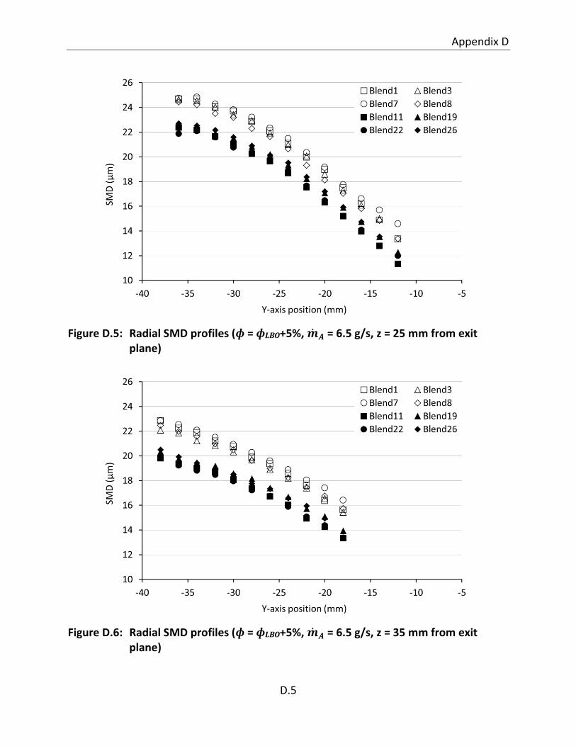
Appendix D
D.5
Figure D.5: Radial SMD profiles (ɸ = ɸLBO+5%, �̇�𝑨 = 6.5 g/s, z = 25 mm from exit plane)
Figure D.6: Radial SMD profiles (ɸ = ɸLBO+5%, �̇�𝑨 = 6.5 g/s, z = 35 mm from exit plane)

PDA Spray Measurement Results
D.6
Figure D.7: Radial SMD profiles (ɸ = 0.6, �̇�𝑨 = 2.2 g/s, z = 15 mm from exit plane)
Figure D.8: Radial SMD profiles (ɸ = 0.6, �̇�𝑨 = 2.2 g/s, z = 25 mm from exit plane)

Appendix D
D.7
Figure D.9: Radial SMD profiles (ɸ = 0.6, �̇�𝑨 = 2.2 g/s, z = 35 mm from exit plane)
Figure D.10: Radial SMD profiles (ɸ = 0.6, �̇�𝑨 = 6.5 g/s, z = 15 mm from exit plane)
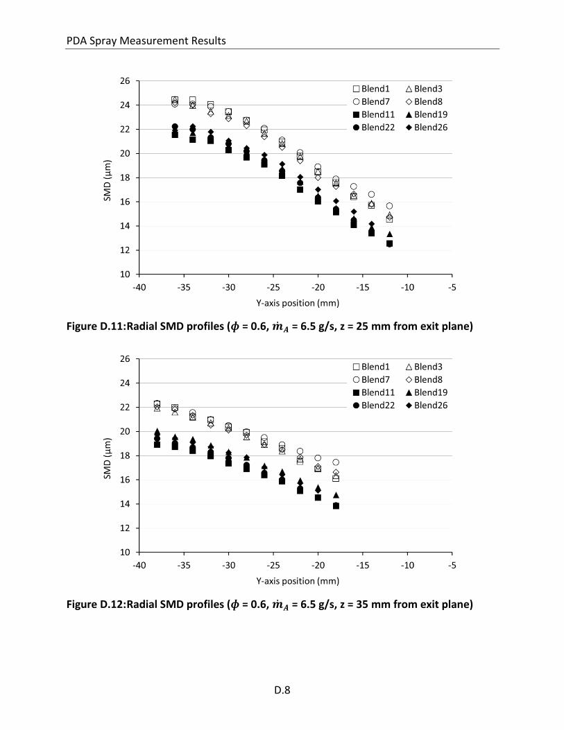
PDA Spray Measurement Results
D.8
Figure D.11: Radial SMD profiles (ɸ = 0.6, �̇�𝑨 = 6.5 g/s, z = 25 mm from exit plane)
Figure D.12: Radial SMD profiles (ɸ = 0.6, �̇�𝑨 = 6.5 g/s, z = 35 mm from exit plane)

E.1
Appendix E: Modelled LBO Air Flow Proportionality Constants
Table E1: Normalised LBO proportionality constants and modified LBO proportionality constants
CJF CJF/D SJF1 SJF2 SJF2+ LTSK HTSK HN
K (A , 323 K) 1.00 1.04 0.88 1.00 0.99 1.08 0.91 0.97
K (B , 323 K) 1.00 1.12 0.93 1.04 1.02 1.09 0.95 1.05
K (A , 413 K) 1.00 0.99 0.93 1.02 0.98 1.12 0.95 1.02
KAve 1.00 1.05 0.91 1.02 1.00 1.10 0.94 1.01
Kθ (A , 323 K) 1.00 1.06 0.81 1.04 0.94 0.93 0.83 0.85
Kθ (B , 323 K) 1.00 1.09 0.88 1.01 0.99 1.02 0.89 0.96
Kθ (A , 413 K) 1.00 0.99 0.93 1.02 1.00 1.12 0.93 1.02
KθAve 1.00 1.05 0.87 1.02 0.98 1.02 0.88 0.94

Modelled LBO Air Flow Proportionality Constants
E.2
Figure E1: Proportionality constants for modelled combustor airflow based on LBO
test data - burner configuration A, 323 K air pre-heat
Figure E2: Proportionality constants for modelled combustor airflow based on LBO
test data - burner configuration A, 413 K air pre-heat

Appendix E
E.3
Figure E3: Proportionality constants for modelled combustor airflow based on LBO
test data - burner configuration B, 323 K air pre-heat
Figure E4: Modified proportionality constants (Kθ) for modelled combustor airflow
based on LBO test data - burner configuration A, 323 K air pre-heat

Modelled LBO Air Flow Proportionality Constants
E.4
Figure E5: Modified proportionality constants (Kθ) for modelled combustor airflow
based on LBO test data - burner configuration A, 413 K air pre-heat
Figure E6: Modified proportionality constants (Kθ) for modelled combustor airflow
based on LBO test data - burner configuration B, 323 K air pre-heat

References
[1] T. Edwards, “Advancements in gas turbine fuels from 1943 to 2005”, Transactions of the ASME, Journal of Engineering for Gas Turbines and Power, vol. 129, pp. 13-20, January 2007.
[2] A. H. Lefebvre, “Fuel effects on gas turbine combustion,” Combustion Laboratory, School of Mechanical Engineering, Purdue University, Indiana, USA, AFWAL-TR-83-2004, January 1983.
[3] United Kingdom. Ministry of Defence, Defence Standard 91-91, Turbine Fuel, Aviation Kerosene Type Jet A-1, NATO Code: F-35, Joint Service Designation: AVTUR, Issue 9, 3 October 2016.
[4] A. H. Lefebvre, Gas Turbine Combustion, 2nd ed. New York: Taylor and Francis, 1999, pp. 50-57.
[5] A. H. Lefebvre, Gas Turbine Combustion, 2nd ed. New York: Taylor and Francis, 1999, p. 35.
[6] C.A. Moses, and P.N. Roets, “Properties, Characteristics and Combustion Performance of SASOL Fully Synthetic Jet Fuel,” in Journal of Engineering for Gas Turbines and Power, 131(4), 2009.
[7] V. Burger, A. Yates, and C. Viljoen, “Influence of Fuel Physical Properties and Reaction Rate on Threshold Heterogeneous Gas Turbine Combustion,” GT2012-68153, in Proceedings of ASME Turbo Expo 2012, Copenhagen, Denmark, 2012.
[8] D. Fyffe, J. Moran, K. Kannaiyan, R. Sadr, and A. Al-Sharshani, “Effect of GTL-like jet fuel composition on GT engine altitude ignition performance – Part I: Combustor operability,” GT2011-45487, in Proceedings of ASME Turbo Expo 2011, Vancouver, Canada, 2011.
[9] V. Burger, A. Yates, T. Mosbach, and B. Gunasekaran, “Fuel influence on targeted gas turbine combustion properties Part II: Detailed results,” GT2014-25105, in Proceedings of ASME Turbo Expo 2014, Düsseldorf, Germany, 2014.
[10] N. Rock, I. Chterev, T. Smith, H. Ek, B. Emerson, D. Noble, J Seitzman, and T. Lieuwen, “Reacting pressurized spray combustor dynamics, Part 1. Fuel sensitivities and blowoff characterization,” GT2016-56346, in Proceedings of ASME Turbo Expo 2016, Seoul, South Korea, 2016.
[11] J. Grohmann, B. Rauch, T. Kathrotia, W. Meier, and M. Aigner, “Investigation of differences in lean blowout of liquid single-component fuels in a gas turbine model combustor,” in Proceedings of 52nd AIAA/SAE/ASEE Joint Propulsion Conference, Salt Lake City, USA, 2016.
[12] C.A. Moses and G. Wilson, “Evaluation of Sasol synthetic kerosene for suitability as jet fuel,” Southwest Research Institute, San Antonio, USA, Report 08-04438, 2003.
[13] C.A. Moses, “Evaluation of Sasol synthetic kerosene for suitability as jet fuel Phase II: Engine and combustor tests,” Southwest Research Institute, San Antonio, USA, Report 08-04438-2, 2007.
[14] F. Hermann, “Cold day ignition and altitude relight testing of Sasol fully synthetic aviation kerosene-External report,” Rolls-Royce, Derby, UK, DNS 126274-2, 2007.
[15] P. Yankowich, “Evaluation of Sasol fully synthetic jet fuel for approval for use as Jet A-1 fuel,” Honeywell Aerospace, Phoenix, USA, 21-13781, 2007.
[16] A. H. Lefebvre, Gas Turbine Combustion, 2nd ed. New York: Taylor and Francis, 1999, pp. 135, 139.

References
[17] G. A. E. Godsave, “Studies of the combustion of drops in a fuel spray – The burning of single drops of
fuel,” in Fourth Symposium (International) on Combustion, The Combustion Institute, 1953, pp. 818-830.
[18] A. H. Lefebvre, Atomization and Sprays. United States of America: Hemisphere Publishing Corporation, 1989, p. 331.
[19] B. J. Wood, H. Wise, and S. H. Inami, “Heterogeneous combustion of multicomponent fuels,” NASA TN D-206, 1959.
[20] J.S. Chin and A. H. Lefebvre, “Effective values of evaporation constant for hydrocarbon fuel drops,” in Proceedings of the 20th Automotive Technology Development Contractor Coordination Meeting, 1982, pp. 325-331.
[21] A. H. Lefebvre, Gas Turbine Combustion, 2nd ed. New York: Taylor and Francis, 1999, pp. 142-145.
[22] A. H. Lefebvre, Gas Turbine Combustion, 2nd ed. New York: Taylor and Francis, 1999, p. 141.
[23] V. W. Greenhough, and A. H. Lefebvre, “Some applications of combustion theory to gas turbine development,” in Sixth Symposium (International) on Combustion, The Combustion Institute, 1957, pp. 858-869.
[24] A. H. Lefebvre, Gas Turbine Combustion, 2nd ed. New York: Taylor and Francis, 1999, pp. 137-141.
[25] A. H. Lefebvre, and G. A. Halls, “Some experiences in combustion scaling,” in AGARD Advanced Aero Engine Testing, AGARD-ograph 37, 1959, pp 177-204.
[26] A. H. Lefebvre, Gas Turbine Combustion, 2nd ed. New York: Taylor and Francis, 1999, p 36-38
[27] J. P. Longwell, E. E. Frost, and M. A. Weiss, “Flame stability in bluff body recirculation zones,” in Journal of Industrial and Engineering Chemistry, Vol. 45, No. 8, 1953, pp. 1629-1633.
[28] R. A. Strehlow, Fundamentals of Combustion, Scranton Pennsylvania, International Textbook Company, 1968, pp. 181-184.
[29] J. E. Penner, D. H. Lister, D. J. Griggs, D. J. Dokken, and M. McFarland, Aviation and the Global Atmosphere. Cambridge, United Kingdom: Cambridge University Press, 1999.
[30] “Standard Atmosphere,” International Organization for Standardization, ISO 2533:1975, 1975.
[31] N. Cumpsty, Jet Propulsion, 2nd ed. Cambridge: Cambridge University Press, 2003, p. 34.
[32] A. Rizkalla and A. H. Lefebvre, “The influence of air and liquid properties on airblast atomization,” in ASME Journal of Fluids Engineering, Vol. 97, No. 3, 1975, pp. 316-320.
[33] A.H. Lefebvre, “Airblast Atomization,” in Progress in Energy and Combustion Science, Volume 6, Number 3, 1980, pp. 233-261.
[34] A. H. Lefebvre, “Fuel effects on gas turbine combustion,” Combustion Laboratory, School of Mechanical Engineering, Purdue University, Indiana, USA, AFWAL-TR-83-2004, 1983.
[35] K. S. Venkataramani, “Aviation fuel property effects on altitude relight,” NASA Lewis Research
Centre, Rep. AD-A183 088, 1987.

[36] H. N. Rao and A. H. Lefebvre, “Minimum ignition energies in flowing kerosine-air mixtures,” in
Combustion and Flame, vol. 27, no.1, 1976, pp. 1-20.
[37] D. R. Ballal and A. H. Lefebvre, “Ignition and flame quenching of quiescent fuel mists,” in
Proceedings of the Royal Society London Ser. A, vol. 364, no 1717, 1987, pp. 277-294.
[38] D. R. Ballal and A. H. Lefebvre, “General model of spark ignition for gaseous and liquid fuel/air
mixtures,” in Eighteenth Symposium (International) on Combustion, 1981, pp. 1737-1746.
[39] A. H. Lefebvre, "Fuel effects on gas turbine combustion-ignition, stability, and combustion efficiency," in ASME Journal of Engineering for Gas Turbines and Power 107: 24-37, 1985.
[40] B. C. Heulskamp, B. V. Kiel, P. Gokulakrishnan, “Influence of fuel characteristics in correlation to predict lean blowout of bluff-body stabilized flames,”GT2015-43433, in Proceedings of ASME Turbo Expo 2015, Montreal, 2015.
[41] S. J. Shanbhogue, S. Husain, and T. Lieuwen, “Lean blowoff of bluff body stabilized flames: Scaling and dynamics,” in Progress in Energy and Combustion Science 35, 2009, pp. 98-120.
[42] K. Radhakrishnan, J.B. Heywood, and R.J. Tabaczynski, “Premixed turbulent flame blowoff velocity correlation based on coherent structures in turbulent flows,” in Combustion and Flame 42, 1981, pp. 19-33
[43] J. Kariuki, D.E. Cavaliere, C. Letty, and E. Mastorakos, “A comparison of the blow-off behaviour of swirl stabilized premixed and spray flames,” 50th AIAA Aerospace Science Meeting, Nashville, USA, 2012.
[44] M. Colket, S. Zeppieri, Z. Dai, and D. Hauptman, “Fuel research at UTRC,” Multi-Agency Coordinating Council for Combustion Research 5th Annual Research Meeting, Livermore, USA, 2012.
[45] S.H. Won, P.S. Veloo, S. Dooley, J. Santner, F.M. Haas, Y. Ju, F.L. Dryer, “Predicting the global combustion behaviours of petroleum-derived and alternative jet fuels by simple fuel property measurements,” in Fuel 168, 2016.
[46] V. W. Greenhough, and A. H. Lefebvre, “Some applications of combustion theory to gas turbine development,” in Sixth Symposium (International) on Combustion, The Combustion Institute, 1957, pp. 858-869.
[47] A. H. Lefebvre, Gas Turbine Combustion, 2nd ed. New York: Taylor and Francis, 1999, pp. 137-141.
[48] A. H. Lefebvre, and G. A. Halls, “Some experiences in combustion scaling,” in AGARD Advanced Aero Engine Testing, AGARD-ograph 37, 1959, pp 177-204.
[49] G. Damkoehler, Z. Elektrochem, 46, 601, 1940.
[50] K.J. Laidler, The development of the Arrhenius equation, in Journal of Chemical Education, 61 (6), 1984, pp.494-498.
[51] A. H. Lefebvre, Gas Turbine Combustion, 2nd ed. New York: Taylor and Francis, 1999, p 36-38
[52] R. A. Strehlow, Fundamentals of Combustion, Scranton Pennsylvania, International Textbook Company, 1968, pp. 181-184.

References
[53] N. Bester, “A test-cell installation of a gas turbine engine to investigate the performance advantages
of low aromatic fuel,” MSc. dissertation, University of Cape Town, Cape Town, South Africa, 2008, p45.
[54] M. A. Weiss, J. C. Roherer, and J. P. Longwell, Sixth Symposium (International) on Combustion, The Combustion Institute, 1957.
[55] R. A. Strehlow, Fundamentals of Combustion, Scranton Pennsylvania, International Textbook Company, 1968, pp. 266-269.
[56] A. H. Lefebvre, Gas Turbine Combustion, 2nd ed. New York: Taylor and Francis, 1999, pp. 48-49
[57] J.B. Heywood, Internal Combustion Engine Fundamentals, McGraw-Hill Book Company, 1988, p. 468.
[58] V. Burger, A. Yates, N. Savage, and O. Metcalf, “Assessment of the Role of Fuel Autoignition Delay at the Limits of Gas Turbine Combustion and Ignition,” GT2009-60332, Proceedings of ASME Turbo Expo 2009: Power for Land, Sea and Air, Orlando, USA. 2009.
[59] United Kingdom. Ministry of Defence, Defence Standard 91-91, Turbine Fuel, Aviation Kerosene Type Jet A-1, NATO Code: F-35, Joint Service Designation: AVTUR, Issue 6, 8 April 2008.
[60] ASTM Standard D1655–11b, Standard Specification for Aviation Turbine Fuels, ASTM International, 2011.
[61] ASTM Standard D2887–08, Standard Test Method for Boiling Range Distribution of Petroleum Fractions by Gas Chromatograph, ASTM International, 2008.
[62] R. van der Westhuizen, M. Ajam, P. de Coning, J. Beens, A. de Villiers, and P. Sandra, “Comprehensive Two-dimensional Gas Chromatography for the Analysis of Synthetic and Crude-derived Jet Fuels,” in Journal of Chromatography A, 1218(28), 2011, pp. 4478-4486.
[63] ASTM Standard D68090 – 13a, Standard Test Method for Determination of Ignition Delay and Derived Cetane Number (DCN) of Diesel Fuel Oils by Combustion in a Constant Volume Chamber, ASTM International, 2013.
[64] A. Yates, V. Burger and C. Viljoen, “A method for determining the laminar flame speed of jet fuels using combustion bomb pressure,” in Proceedings of ASME Turbo Expo 2012: Power for Land, Sea and Air, GT2012, Copenhagen, Denmark, June 11-15, 2012.
[65] J. Grohmann, W. O’Loughlin, W. Meier, and M. Aigner, “Comparison of the Combustion Characteristics of Liquid Single-component Fuels in a Gas Turbine Model Combustor,” GT2016-56177, in Proceedings of ASME Turbo Expo 2016: Turbomachinery Technical Conference and Exposition, Seoul, South Korea, 2016.
[66] A. H. Lefebvre, and D. R. Ballal, Gas turbine combustion: alternative fuels and emissions, CRC Press, Taylor and Francis Group, 2010.
[67] D. Galley, S. Ducruix, F. Lacas, and D. Veynante, “Mixing and stabilization study of a partially premixed swirling flame using laser induced fluorescence” in Combustion and Flame, 158(1), 2011 pp. 155–171.
[68] A. H. Lefebvre, Gas Turbine Combustion, 2nd ed. New York: Taylor and Francis, 1999, p 127.

[69] ASTM Standard D68090 – 13a, Standard Test Method for Determination of Ignition Delay and
Derived Cetane Number (DCN) of Diesel Fuel Oils by Combustion in a Constant Volume Chamber, ASTM International, 2013.
[70] A. D. B. Yates, C. L. Viljoen, A. Swarts, “Understanding the relation between cetane number and combustion bomb ignition delay measurements”, SAE 2004-01-2017, 2004.
[71] W. Zeng, H. Ma, Y. Liang, E. Hu, “Experimental and modelling study on effects of N2 and CO2 on ignition characteristics of methane/air mixture,” in Journal of Advanced Research 6, Cairo University, 1998, p.371-378.
[72] A. H. Lefebvre, Gas Turbine Combustion, 2nd ed. New York: Taylor and Francis, 1999, p. 45.