Combustion, Flames and CFD

Rudolf Žitný, Ústav procesní a zpracovatelské techniky ČVUT FS 2010

HEAT PROCESSESHP11

CFD analysis of combustion. Transport equations and modeling of chemical reactions. Non-premix combustion and mixture fraction methods. Lagrangian and Eulerian methods.

HP11 Combustion and Flames

Mark Bradford

Warnatz J.: Combustion. Springer, Berlin 1996

Homogeneous reaction in gases

Premixed (only one inlet stream of mixed fuel and oxidiser)

Non premixed (separate fuel and oxidiser inlets)

Laminar flame

Turbulent flame

Laminar flame

Turbulent flame

Use mixture fraction method

(PDF)

Use EBU (Eddy Break Up models)

Liquid fuels (spray combustion)

Combustion of particles (coal)

Lagrangian method-trajectories of a representative set of droplets/particles

in a continuous media

Lagrangian method-trajectories of a representative set of droplets/particles

in a continuous media

HP11 Combustion

Premixed combustion

Fuel and oxidiser are mixed first and even then burn

HP11 Combustion

Laminar premixed flames are characterised by a narrow flame front (front width depends upon the rate of chemical reaction and diffusion coefficient). Laminar burning velocity (uL) must be greater than the velocity of flow (um) in case of a flat flame front, otherwise the flame will be extinguished (in fact this is the way how to determine the burning velocity experimentally). Example: flat laminar flame in porous ceramic burner. Nonuniform transversal velocity profile is manifested by a conical flame front, and the flame front cone angle depends upon burning velocity uL=um sin . Example: Bunsen burner.

In case of turbulent flow the flame front is wavy and fluctuating (flamelets, the turbulent flame can be viewed as an ensemble of premixed laminar flames). Example: Combustion in a cylinder of spark ignition engine, gas turbines in power plants.

Advantage of the premixed combustion: In a gas turbine operating at a fuel-lean condition high temperatures and associated NOx formation are avoided. Soot formation is also suppressed. Disadvantage: Risk of uncontrolled explosion of premixed reactants.

flameletsflamelets

Turbulent premixed flameuL burning velocity (=umsin)

flame frontflame front

um

Bunsen laminar flame

um

porous plate

Flat flame

Bunsen burner fully premixed. Colour corresponds to radicals CH (photo Wikipedia)

R.N. Dahms et al. / Combustion and Flame (2011)

HP11 CombustionNonpremixed combustion

Fuel and oxidiser enter combustion chamber as separated streams. Mixing and burning take place simultaneously (nonpremix is called diffusive burning).

Turbulent nonpremixed flame

fuel+flue gas

air+flue gas

air

stoichiometric line

Laminar nonpremixed flame

Flame front

fuel air

Burned gases

Nonpremixed flames unlike premixed flames do not propagate. Flame simply cannot propagate into the fuel side because there is no oxygen, neither to the oxidising region with lack of fuel. Only burned products diffuse to both sides of the flame front. Flame front position corresponds to stoichiometric ratio fuel/air – there is also the highest temperature.

In turbulent nonpremixed flames the flamelet concept can be used again. Chemistry of nonpremixed combustion is more complicated because on one side of the flame front is the fuel-rich burning accompanied by formation of sooth and on the air side a fuel lean combustion occurs. Existence of glowing sooth is manifested by yellow luminiscence.

Examples: Industrial burners, combustion engines.

Laminar coflow (left) counter flow (right).

HP11 Combustion-flame

Previous lecture HP10 was devoted to statics (fuel consumption, overall mass and enthalpy balances,…). Questions like: What is the distance of the flame front disc levitating above a porous ceramic plate? What is the thickness of the flame front? What is the burning velocity? Which species are generated inside the flame? Concentration profiles? Temperature profiles? What is the height and width of the flame?... should be addressed to kinetics.

Flame propagation

An idea about processes related to burning velocity and flame propagation can be obtained from analysis of the simplest 1D cases. There is a similarity with drying: process is again controlled by diffusion (now diffusion of fuel and products of burning), and heat fluxes are consumed at a moving interface (flame front, now the enthalpy changes of chemical reaction substitute the enthalpy of phase changes).

On the other hand the problem is more difficult, because there are much more transported species and chemical reactions strongly depend upon temperature. Transport equations are therefore nonlinear and numerical solution is necessary.

HP11 Combustion-flame… and numerical solution is necessary. There are few exceptions: Zeldovic and Frank-Kamenetskii (1938) described the flame propagation of a steady premixed planar flame by a transport equation of fuel (mass fraction F(z)) and by transport equation for enthalpy (temperature T(z)) assuming first-order chemical reaction (fuelproduct) and similarity of transport equations (assuming that the diffusion coefficient D is approximately the same as the temperature diffusion coefficient a). Analysis of these equations reveals the fact that a steady solution (stationary position of the flame front) exists only as soon as the flow velocity u (=uF flame velocity) is

uF

T-temperature

F - fuelz

10 20 [mm]

)exp(

1

RTE

A

Du

reaction

reaction

diffusionF

Result: The flame velocity increases when the diffusion coefficient or the chemical reaction rate increases.

E is activation energy and A preexponential factor

characterising rate of the chemical reaction (Arrhenius term).

HP11 Combustion-flame

0)(1 2

2

rrD

rrfuel

dif

R

r

Some information about the flame front can be obtained from the solution of diffusion equation. For example the flame front position around the burning fuel particle in air can be estimated from the radial mass fraction profiles obtained by solution of the diffusion equation

fueĺ=1 ox=1

r

R

r

rRRr oxfuel

1 )(

)(

R

Dm

R

RDm dif

oxdif

fuel )(

…and now: position of front (distance ) is determined by stoichiometry of chemical reaction (1 kg of fuel consumes s kg of oxidiser), therefore and assuming the same diffusion coefficient in fuel and in air

fuel oxsm m

/R s

all fuel is consumed in the thin flame front

HP11 Combustion-flameFlame size

The size (length) of a nonpremixed burning jet can be estimated from the velocity of jet and from the diffusion time necessary for mixing in the transversal direction. Burke and Schumann (1928), Ind.Eng.Chem 20:998

hr-mixing length

Velocity of circular jets decreases with the distance from nozzle (u~1/x) however this approximation assumes a constant velocity at axis and also cylindrical form of jet, having radius r of fuel nozzle. Mixing length (r) is associated with the mixing time by theory of penetration depth

tDr difand the height of flame h is estimated as the product of the mixing time and axial velocity

dif

fuel

dif

fuelfuel

D

V

D

r

r

Vt

r

Vuth

2

2

22

This is qualitatively correct conclusion stating that the flame length is proportional to flowrate and indirectly proportional to diffusion coefficient (Warnatz 1996 documents the diffusion coefficient effect by comparing the height of flame at hydrogen combustion that is 2.5 shorter than the flame height at carbon monoxide combustion)

HP11 Combustion-flame-explosion

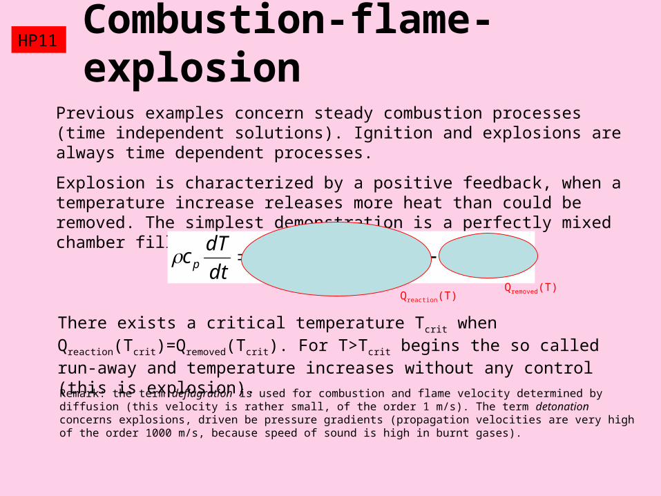
Previous examples concern steady combustion processes (time independent solutions). Ignition and explosions are always time dependent processes.

Explosion is characterized by a positive feedback, when a temperature increase releases more heat than could be removed. The simplest demonstration is a perfectly mixed chamber filled by reaction mixture (Semenov 1928)

)()exp( wa

reactionp TTSRT

EAh

dt

dTc

Qreaction(T)Qremoved(T)

There exists a critical temperature Tcrit when Qreaction(Tcrit)=Qremoved(Tcrit). For T>Tcrit begins the so called run-away and temperature increases without any control (this is explosion).

Remark: the term deflagration is used for combustion and flame velocity determined by diffusion (this velocity is rather small, of the order 1 m/s). The term detonation concerns explosions, driven be pressure gradients (propagation velocities are very high of the order 1000 m/s, because speed of sound is high in burnt gases).

HP11 Chemical reactions

HP11 Rate of chemical reactionsWhen discussing combustion statics a detailed knowledge of actual chemical reactions is not needed – released heat can be evaluated only from the composition of fuel and burned gas (this composition can be obtained for example by analyzers of flue gas). This is because according to the Hess’s law the enthalpy change of a reaction (enthalpy of products minus enthalpy of reactants) is independent of a specific reaction mechanism:

0 0 0298 , 298 , 298

enthalpy released by combustionof moles of reactants

( ) ( ) ( )

R

r P f P R f RP R

h h h

where are stoichiometric coefficients of reactants (R) and products (P), is the standard enthalpy of formation corresponding to the formation of compound from elements in their standard state (at temperature 298 K and atmospheric pressure).

What is substantial: It is sufficient to evaluate only the overall chemical reaction and it is not necessary to sum up reaction enthalpies of many actual elementary reactions.

R P 0 0,(

~),h f compound

0298

Combustion of MethaneExample: Gas burner operating at atmospheric pressure consumes mass flowrate of CH4 0.582 kg/s. Calculate mass flowrate of flue gas. Assuming temperature of fuel and air 298K and temperature of flue gases 500 K calculate heating power.

4 2 2

4 2 2 2

0 0 0, 298 , 298 , 298

1, 2, 1, 2

( ) 75, ( ) 393, ( ) 242

2 24 2 2 2

CH O CO H O

f CH f CO f H Oh h h

CH O CO H O

4

00 0 298

298 , 298 4

( ) 802( ) ( ) 75 1 393 2 242 802 / 50

0.016R

R i f i Ri CH

h MJh h kJ mol CH h

M kg

Flue gas production 1kg CH4 needs 4 kg O2. Mass fraction of oxygen in air is 0.233.

2 2

4 2 2 4 2 4

2 2

0.767(1 ) (5 4 ) 0.582(5 4 ) 10.57 /

0.233N N

fg CH O N CH O CHO O

m m m m m m m kg s

Heat removed

4 0( ) 50 0.582 0.01057 (500 298) 27R CH fg p fgQ h m m c T T MW

cp0.001 MJ/kgK

Air

CH4

fg-flue gasQ

HP11

Remark: methane combustion is described by more than 200 elementary chemical reactions. Because we need only overall heat it is sufficient to use only one overall chemical reaction.

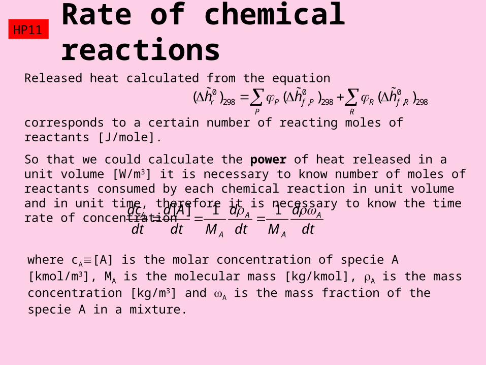
HP11 Rate of chemical reactionsReleased heat calculated from the equation

corresponds to a certain number of reacting moles of reactants [J/mole].

So that we could calculate the power of heat released in a unit volume [W/m3] it is necessary to know number of moles of reactants consumed by each chemical reaction in unit volume and in unit time, therefore it is necessary to know the time rate of concentration

0 0 0298 , 298 , 298( ) ( ) ( )r P f P R f R

P R

h h h

dt

d

Mdt

d

Mdt

Ad

dt

dc A

A

A

A

A 11][

where cA[A] is the molar concentration of specie A [kmol/m3], MA is the molecular mass [kg/kmol], A is the mass concentration [kg/m3] and A is the mass fraction of the specie A in a mixture.

HP11 Rate of chemical reactionsIf we need to calculate the composition inside a flame and the composition of flue gas or if it is necessary to evaluate temperature distribution inside a combustion chamber, the rate of chemical reactions must be known.

Reaction rate of a general reaction A+B+… D+E+… can be expressed ask

...][][][ ba BAk

dt

Ad

where [A] is molar concentration of the specie A [kmol/m3], exponents a,b,… are reaction orders with respect to the species A,B,… (only reactants, not products!) and the sum of all exponents a+b+…=n is the overall reaction order. K is the rate coefficient of reaction that depends upon temperature and pressure.

Example:

Combustion of hydrogen with chlorine H2+Cl22HCl

Reaction is of the first order with respect to hydrogen and of order 0.5 with respect to chlorine (overall reaction order n=1.5).

5.022 ]][[

][ClHk

dt

HCld

HP11 Rate of chemical reactionsPrevious example demonstrates that the reaction orders need not be integers, they are usually rational, sometimes even negative, numbers. Even worse: the rate equation of overall chemical reaction has a limited validity, reaction orders and reaction coefficients depend upon temperature and pressure. The reason for this complicated behavior is in complexity of chemical reactions. Overall reactions should be decomposed to several elementary reactions, and in the previous case instead of H2+Cl22HCl the following set of four elementary reactions should be considered.

1

2

3

4

2

2

2

2

2

2 Cl

k

k

k

k

Cl Cl

Cl

Cl H HCl H

H Cl HCl Cl

Elementary reactions can be either unimolecular (for example the reaction 1, decomposition of Cl2 molecule to radicals Cl) or bimolecular (reactions 2,3,4). Unimolecular elementary reactions are always of the first order (reaction exponent a=1) and bimolecular are of the second order (exponents a=b=1). Actual rate of overall chemical reaction is evaluated by simultaneous solution of the four differential equations with the rate coefficients k1,k2,k3,k4. Solution of these differential equations can be simplified by assuming that the radicals Cl and H are at chemical equilibrium and the time derivatives of their concentration can be neglected. Then the differential equations describing the time changes of radicals reduce to algebraic equations and the concentration of [H] and [Cl] can be eliminated from the set of elementary reactions. Rate equations are therefore expressed only in terms of [Cl2] and [H2], giving previously presented result 5.0

22 ]][[][

ClHkdt

HCld

Remark: Not all bimolecular reactions are elementary reactions (H2+Cl22HCl is an example). Elementary bimolecular reactions are characterized by presence of highly reactive radicals as reactants.

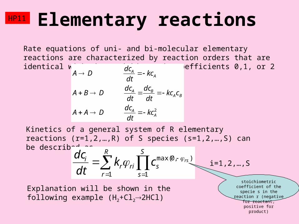
HP11 Elementary reactionsRate equations of uni- and bi-molecular elementary reactions are characterized by reaction orders that are identical with the stoichiometric coefficients 0,1, or 2

2

AA

BABA

AA

kcdt

dcDAA

ckcdt

dc

dt

dcDBA

kcdt

dcDA

Kinetics of a general system of R elementary reactions (r=1,2,…,R) of S species (s=1,2,…,S) can be described as

S

ss

R

rrir

i rsckdt

dc

1

),0max(

1

i=1,2,…,S

Explanation will be shown in the following example (H2+Cl22HCl)

stoichiometric coefficient of the specie s in the reaction

r (negative for reactant, positive for product)

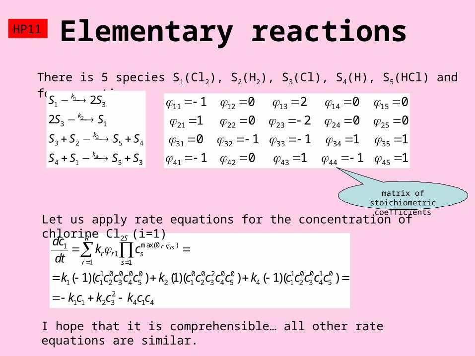
HP11 Elementary reactionsThere is 5 species S1(Cl2), S2(H2), S3(Cl), S4(H), S5(HCl) and four reactions

1

2

3

4

1 3

3 1

3 2 5 4

4 1 5 3

2

2

k

k

k

k

S S

S S

S S S S

S S S S

max(0, )11

1 1

1 0 0 0 0 0 0 2 0 0 1 0 0 1 01 1 2 3 4 5 2 1 2 3 4 5 4 1 2 3 4 5

21 1 2 3 4 1 4

( 1)( ) (1)( ) ( 1)( )

rs

SR

r r sr s

dck c

dt

k c c c c c k c c c c c k c c c c c

k c k c k c c

11101

11110

00201

00201

4544434241

3534333231

2524232221

1514131211

Let us apply rate equations for the concentration of chlorine Cl2 (i=1)

matrix of stoichiometric coefficients

I hope that it is comprehensible… all other rate equations are similar.

HP11 Temperature dependenceReaction constants k depend upon temperature according to Arrhenius law

aE

RTk Ae

Activation energy of chem.reaction

J/mol

Preexpontial factor (the same unit as k)

Relative amount of molecules having kinetic energy greater than Ea is given by Maxwell distribution of energies /E RTe

The greater is temperature the more molecules have energy greater than E

Collision theory: only the molecules having energy greater than Ea react at mutual collision.

Reactions having high activation energy proceed at high temperatures and vice versa (thermal NOx reaction with Ea~300 kJ/mol starts at about 1500 K, while prompt NOx reaction with Ea~100 kJ/mol is important at relatively low temperature about 1000 K)

HP11 Simplified reaction mechanismReality is such that even the simple looking reaction like hydrogen combustion 2H2+O22H2O requires about 40 elementary reactions for a satisfactory reaction mechanism. Combustion of hydrocarbons is even more complicated and is represented by hundreds and thousands of elementary reactions (oxidation of the simplest hydrocarbon CH4 is described by 277 reactions among 49 chemical species). Simultaneous solution of thousands differential equations is too expensive for simulation of practical systems with 3 dimensional inhomogeneous turbulent flows. There exist several techniques how to reduce the complicated system, generally based upon exclusion of reactions that are very fast and are in partial equilibrium (QSSA Quasi-Steady-State-Assumption, ILDM Intrinsic Low Dimensional Method, see Peters 2000). Methane oxidation can be in this way reduced to global mechanism consisting in only four or even two steps

22

224

2

1

22

3

COOCO

OHCOOCH

HP11

Simplified reaction mechanisms are applied also for description of NOx formation (important for design of burners from the point of view of emissions). While the concentrations of CO2, H2O can be predicted by assuming equilibrium, NO reactions are slow and far from equilibrium at short residence times in burning zone (some ms, time scales of reactions are thousand times longer).

Thermal NOx (Zeldovic mechanism)

Prompt NOx (Fenimore)

Fuel NOx

Simplified reaction mechanism

HNOOHN

ONOON

NNONO

k

k

k

3

2

1

2

2Source of NO from atmospheric nitrogen formed by the following reactions:

The first reaction (attack of oxygen radical to N2) has very high activation energy (319 kJ/mol) and proceeds only at very high temperatures.

Prompt NO is formed also from atmospheric N2 but at the flame front from radicals CH (fuel rich flame) NONHCNNCH ...2

Fuel-bound nitrogen is converted into NO mainly in coal combustion (there is approximately 1% chemically bound N in coal) ONNON

HNOOHN

2

CFD - TURBULENT FLAMESHabisreuter P. et al. Mathematical modeling of turbulent swirling flames in Cox M.et al: Combustion Residues: Current, Novel and Renewable Applications. J.Wiley 2008

CFD - THERMOCHEMISTRYKubota, N. (2007) Combustion Wave Propagation, in Propellants and Explosives: Thermochemical Aspects of Combustion, Wiley Weinheim

HP11 CFD models

CFD - TURBULENT COMBUSTIONPeters N.: Turbulent combustion. Cambridge Univ.Press, 2000

Alexander

HP11 Flow modelling – Navier Stokes

( ) 0ut

( ) m

Dup u s

Dt

Combustion modelling is always based upon the solution of Navier Stokes equations for vector of velocity field (even if it is combustion of liquid or solid fuels). There are 4 unknowns: 3 components of velocity ux,uy,uz and pressure. Therefore 4 partial differential equations must be solved simultaneously

Continuity equation, stating that the accumulation of mass is the divergence of mass flux

Momentum balance, stating that the mass x acceleration equals the sum of forces acting upon a fluid element (pressure forces + viscous forces + volumetric forces)

Solution of these equations (velocity field) describes convective transport of fuel, oxidiser as well as products of burning inside a combustion chamber. These equations are quite general, describe incompressible/compressible fluids, laminar as well as turbulent flow regime, but…

HP11 Flow modelling – Navier Stokes

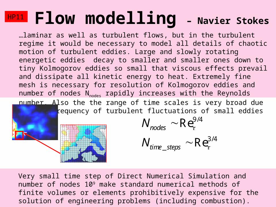
…laminar as well as turbulent flows, but in the turbulent regime it would be necessary to model all details of chaotic motion of turbulent eddies. Large and slowly rotating energetic eddies decay to smaller and smaller ones down to tiny Kolmogorov eddies so small that viscous effects prevail and dissipate all kinetic energy to heat. Extremely fine mesh is necessary for resolution of Kolmogorov eddies and number of nodes Nnodes rapidly increases with the Reynolds number. Also the the range of time scales is very broad due to high frequency of turbulent fluctuations of small eddies (10 kHz).

9/4

3/4_

Re

Re

nodes

time steps

N

N

Very small time step of Direct Numerical Simulation and number of nodes 109 make standard numerical methods of finite volumes or elements prohibitively expensive for the solution of engineering problems (including combustion).

HP11

The most frequently used technique for modeling of turbulent flows consists in averaging of fluctuating quantities (velocities, density, pressure, temperature and concentrations). Filtration of time fluctuations (substituting actual noisy time course at a point x,y,z by average) is the principle of RANS (Reynolds Averaging Navier Stokes) family of numerical methods while the spatial fluctuations filtering is a characteristic of LES (Large Eddy Simulation) class.

It is assumed that filtering the time fluctuations smooth out the spatial fluctuations and vice versa (because turbulent fluctuations are correlated).

/2

/2

( ) ( , ) /t

t

u x u x d

Δ t

u

'uuu

Turbulent flow RANS/LES

Mean value

Temporary fluctuation

HP11

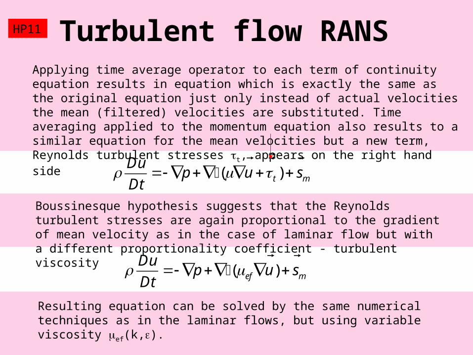
Applying time average operator to each term of continuity equation results in equation which is exactly the same as the original equation just only instead of actual velocities the mean (filtered) velocities are substituted. Time averaging applied to the momentum equation also results to a similar equation for the mean velocities but a new term, Reynolds turbulent stresses t, appears on the right hand side

Turbulent flow RANS

( )t m

Dup u s

Dt

( )ef m

Dup u s

Dt

Boussinesque hypothesis suggests that the Reynolds turbulent stresses are again proportional to the gradient of mean velocity as in the case of laminar flow but with a different proportionality coefficient - turbulent viscosity

Resulting equation can be solved by the same numerical techniques as in the laminar flows, but using variable viscosity ef(k,).

HP11 Turbulent flow RANS k-

2

t

kC

Effective viscosity can be expressed as the sum of actual (molecular) viscosity and turbulent viscosity t representing momentum transport by turbulent eddies. This contribution (t) depends upon the magnitude of velocity fluctuation (or square of this magnitude, expressed by the kinetic energy of turbulence k [m2/s2]) and also upon the rate of how the kinetic energy of turbulent eddies is converted to smaller eddies and in the final instance to heat. This second characteristic is the dissipation of energy of turbulence [m2/s3] (the unit of follows from the unit of k, because is the change of k per second).

Turbulent viscosity can be expressed by the model

where C is a constant (usually 0.09). There is no mystery in the correlation: it can be derived easily by dimensional analysis (unit of viscosity is Pa.s) assuming power law formula and comparing exponents at kg, m, st k

2 2 2 2 3

2 3 3 2 2 3[ . ] [ ][ ][ ]

Ns kg kg m m kg mPa s

m ms m s s s

1

1 2 2 3

1 2 3

1

1

2

HP11 Turbulent flow RANS k-

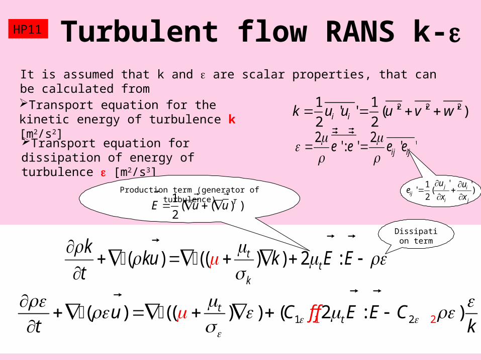
1 221( ) (( ) ) ( 2 : )ttu C E E C

t kf f

( ) (( ) ) 2 :tt

k

kku k E E

t

2 2' : ' ' 'ij ije e e e

2 2 21 1' ' ( ' ' ' )

2 2i ik u u u v w Transport equation for the kinetic energy of turbulence k [m2/s2]

Transport equation for dissipation of energy of turbulence [m2/s3]

Production term (generator of turbulence)

Dissipation term

' '1' ( )

2j i

iji j

u ue

x x

1( ( ) )

2TE u u

It is assumed that k and are scalar properties, that can be calculated from

HP11 Turbulent flow RANSThe choice k- and the two transport equations for k and is not by far the only way how to characterize a state of turbulence.Two equation models calculate turbulent viscosity from the pairs of turbulent characteristics k-, or k-, or k-l (Rotta 1986)

k (kinetic energy of turbulent fluctuations) [m2/s2]

(dissipation of kinetic energy) [m2/s3]

(specific dissipation energy) [1/s]

l (length scale) [m]

2

t

t

k

kC

Wilcox (1998) k-omega model, Kolmogorov (1942)

Jones,Launder (1972), Launder Spalding (1974) k-epsilon model

These pairs of turbulent characteristics can describe not only the turbulent viscosity but also transport coefficients (diffusivity, thermal conductivity) and the rate of micromixing Rm (kg of component mixed in unit volume per second) that controls the rate of combustion, e.g.

CR

kCR mm

as follows from dimensional analysis (the

same way as turbulent viscosity)

HP11 Turbulent flow RANS

All the presented CFD RANS models (and many others), are available in commercial programs like Fluent.

Knowing velocity field and scalar characteristics of turbulence it is possible to analyzed transport of individual species, chemical reactions, and temperatures…

i mass fraction of specie i in mixture [kg of i]/[kg of mixture] i mass concentration of specie [kg of i]/[m3]

Mass balance of species (for each specie one transport equation)

( ) ( ) ( )i i i i iut

S

Rate of production of specie i [kg/m3s]Production of species is controlled by

Diffusion of reactants (micromixing) – tdiffusion (diffusion time constant)

Chemistry (rate equation for perfectly mixed reactants) – treaction (reaction constant)

Damkohler numberdiffusion

reaction

tDa

t

exp( ) ai i

i i

ES A

RT

S Ck

Da<<1

Da>>1

Reaction controlled by kinetics (Arrhenius)

Turbulent diffusion controlled combustion

Because only micromixed reactants can react

HP11 Combustion – mass balances

HP11 Combustion – mass balances

max(0, )

1 1

rs

SRi

i i r ri sr s

dS M k c

dt

The source term Si [kg/(m3s)] is the sum of contributions of all chemical reactions where the specie i exists either as a reactant or a product (when stoichiometric coefficient ri of specie i in reaction r is nonzero)

S-is number of species (i=1,2,…,S) and R is number of chemical reactions.

Enthalpy balance is written for mixture of all species (result-temperature field)

( ) ( ) ( ) hh h Su ht

Sum of all reaction enthalpies of all reactions

,

enthalpy of formation

/h i f i ii

S S h M

It holds only for reaction without phase changes h ~ cpT

Energy transport must be solved together with the fluid flow equations (usually using turbulent models, k-, RSM,…). Special attention must be paid to radiative energy transport (not discussed here, see e.g. P1-model, DTRM-discrete transfer radiation,…). For modeling of chemistry and transport of species there exist many different methods but only one - mixture fraction method for the non-premixed combustion will be discussed in more details.

HP11 Combustion - enthalpy

3 3

,

kg/kmolenthalpy of W/m kg/(m s)formation J/kmol

/h i f i ii

S S h M

HP11 Combustion - enthalpy

The production term Sh [W/m3] is the sum of reaction enthalpies over all exo- or endothermic reactions.

It can be calculated from a simplified reaction scheme (from reduced number of overall reactions, reaction enthalpies and reaction progresses of these reactions) but also from the previously calculated Si values (kg of specie i generated in unit volume and unit time due to all chemical reactions) and corresponding enthalpies of formation

HP11 Mixture Fraction method

Bingham

Let us consider non-premixed combusion, and fast chemical reactions (paraphrased as “What is mixed is burned (or at equilibrium)”)

mfuel

moxidiser

Flue gases

Mass balance of fuel

Mass balance of oxidant

( ) ( ) ( )fuel fuel fuel fuelu St

( ) ( ) ( )ox ox ox oxu St

Calculation of fuel and oxidiser consumption is the most

difficult part. Mixture fraction method is the way, how to

avoid it

3

of produced fuel[ ]kg

s m

Mass fraction of oxidiser (e.g.air)

Mass fraction of fuel (e.g.methane)

HP11 Mixture Fraction method

Stoichiometry

1 kg of fuel + s kg of oxidiser (1+s) kg of product

and subtracting previous equations( ) ( ) ( )

( ) ( ) ( )

fuel fuel fuel fuel

ox ox ox ox

s s s su St

u St

( ) ( ) ( ) fuel oxsu S St

Introducing new variable

fuel oxs

This term is ZERO due to stoichimetry

HP11 Mixture Fraction method

-Sfuel is kg of fuel consumed in unit volume per one second (at a given place x,y,z and time t).

Mixture fraction f is defined as linear function of normalized in such a way that f=0 at oxidising stream and f=1 in the fuel stream

Resulting transport equation for the mixture fraction f is without any source term

( ) ( ) ( )f fu ft

,00

1 0 ,1 ,0

fuel ox ox

fuel ox

sf

s

Mixture fraction is a property that is CONSERVED, only dispersed and transported by convection. f can be interpreted as a concentration of a key element (for example carbon). And because it was assumed that „what is mixed is burned“ the information about the carbon concentration at a place x,y,z bears information about all other participating species, see next slide…

ox is the mass fraction of oxidiser at an arbitrary point

x,y,z, while ox,0 at inlet (at the stream 0)

HP11 Mixture Fraction method

Knowing f we can calculate mass fraction of fuel and oxidiser at any place x,y,z

,0

,1 ,0

oxst

fuel oxoichiof

s

For example the mass fraction of fuel is calculated as

ox ,1(fuel rich region, oxidiser is consumed =0) 1 1

stoichiostoichio

stoichiofuel fuel

f

ff

ff

(fuel lean region) 0 0stoichio fuelff

The concept can be generalized assuming that chemical reactions are at equlibrium

f → i mass fraction of species is calculated from equilibrium constants

(evaluated from Gibbs energies)

At the point x,y,z where f=fstoichio are all reactants consumed

(therefore ox=fuel=0)

HP11 Mixture Fraction method

Equilibrium depends upon concentration of the key component (upon f) and temperature. Mixture fraction f undergoes turbulent fluctuations and these fluctuations are characterized by probability density function p(f). Mean value of mass fraction, for example the mass fraction of fuel is to be calculated from this distribution

1

0

( ) ( )fuel fuel f p f df

Mass fraction corresponding to an arbitrary value of mixture fraction is calculated from equlibrium constant

Probability density function, defined in terms of mean and variance of f

0 fmean 1

p

Frequently used distribution1 1

11 1

0

(1 )( )

(1 )

p q

p q

f fp f

f f df

Variance of f is calculated from another transport equation

2 2 2 2 2( ' ) ( ' ) ( ' ) ( ) 'f g t df f u f C f C ft k

HP11 Mixture Fraction method

Final remark: In the case, that fuel is a linear function of f, the mean value of mass fraction fuel can be evaluated directly from the mean value of f (and it is not necessary to identify probability density function p(f), that is to solve the transport equation for variation of f). Unfortunately the relationship fuel(f) is usually highly nonlinear.

1

0

( ) ( ) ( )fuel fuel fuelf p f df f

HP11 Mixture Fraction method

mfuel

1| | ( )

2D D

dum F

dt

F c A u v u v

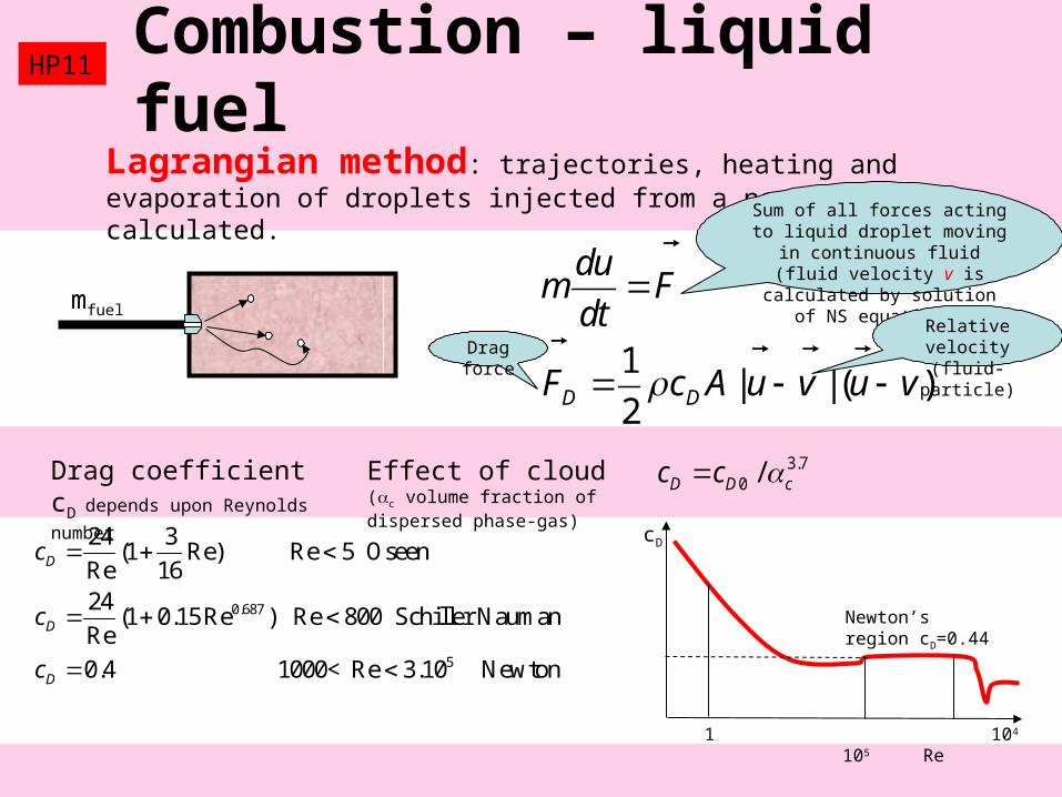
Lagrangian method: trajectories, heating and evaporation of droplets injected from a nozzle are calculated. Sum of all forces acting to liquid

droplet moving in continuous fluid (fluid velocity v is calculated

by solution of NS equations)

Relative velocity (fluid-particle)Drag force

Drag coefficient cD depends upon Reynolds number

0.687

5

24 3(1 Re) Re 5 Oseen

Re 1624

(1 0.15Re ) Re 800 Schiller NaumanRe

0.4 1000< Re 3.10 Newton

D

D

D

c

c

c

1 104 105 Re

cD

Newton’s region cD=0.44

Effect of cloud (c volume fraction of dispersed phase-gas)

3.70 /D D cc c

HP11 Combustion – liquid fuel

Evaporation of fuel droplet

Diffusion from droplet surface to gas:

22

05 0.33

( ) ( )6

2 0.6Re

p g dif fg s

dm d DD Sh D m m

dt dt

Sh Sc

Mass fraction of fuel at surface

Sherwood number

Schmidt number =/Ddif

Ranz Marshall correlation for mass transport

HP11 Combustion – liquid fuel

difD

DSh

CFD examples

Vít Kermes, Petr Belohradský, Jaroslav Oral, Petr Stehlík: Testing of gas and liquid fuel burners for power and process industries. Energy, Volume 33, Issue 10, October 2008, Pages 1551-1561

Lempicka

HP11 CFD – gas burner

HP11 CFD – gas burner

Zeldovic NOx – thermal NOx

HP11 CFD – gas burner

HP11 CFD – gas burner

• Low computational cost CFD analysis of thermoacoustic oscillationsApplied Thermal Engineering, Volume 30, Issues 6-7, May 2010, Pages 544-552Andrea Toffolo, Massimo Masi, Andrea Lazzaretto

Timing of the pressure fluctuation due to the acoustic mode at 36 Hz and of the heat released by the fuel injected through the main radial holes (if the heat is released in the gray zones, the necessary condition stated by Rayleigh criterion is satisfied and thermoacoustic oscillations at this frequency are likely to grow).

HP11 CFD thermoacoustic burner

HP11

EXAMHP11

Combustion chemistry and CFD

What is important (at least for exam)HP11

0 0 0

298 , 298 , 298

0products (with positive enthalpy of formationstoichiometric coefs. ) at standard pressure

and temperature 298K

( ) ( ) ( )R

P

r P f P R f RP R

h h h

Heat released by reaction of reactants with stoichiometric coefficients R

max(0, )

1 1

1rs

SRi i

r ri sr si

dc dk c

dt M dt

stoichiometric coefficient of the specie s in the reaction

r (negative for reactant, positive for product)

Kinetics of R- elementary chemical reactions (ci is molar concentration of specie i). This rate equation holds only for elementary reactions (mono and bimolecular reactions) and not for overall reactions.

HNOOHN

ONOON

NNONO

k

k

k

3

2

1

2

2

Example: complicated reaction mechanism of NO formation from atmospheric nitrogen can be simplified to only 3 elementary bimolecular reactions (Zeldovic mechanism of NOx formation)

OHNONNONO cckcckcckdt

dc321 22

reaction constant depends upon temperature (Arrhenius term

~exp(-Er /RT), where Er is activation energy of reaction r)

What is important (at least for exam)HP11

reaction heat correspondingto all chemical reactions

( ) ( ) hShu h

production of specie iconvective transport diffusion by turbulent eddies

( ) ( )i i i iu S

Concentration of species ci (or mass fractions i) in the combustion chamber follows from the mass balance (transport equation for specie i)

max(0, )

1 1

rs

SRi

i i r ri sr s

dS M k c

dt

The source term Si corresponds to all chemical reactions where the specie i exists either as a reactant or a product (when stoichiometric coefficient ri is nonzero)

Temperature field follows from enthalpy balance where all chemical equations (and their reaction enthalpies) should be included

What is important (at least for exam)HP11

CFD (Computer Fluid Dynamics) solution is based upon numerical solution of previous transport equations for concentrations (or i) and temperatures (or enthalpies h) together with the Navier Stokes equations and continuity equation for velocity and pressure. In case of turbulent flow it is necessary to solve also additional transport equation for turbulent characteristics (for example k and ).

This complicated system of partial differential equations can be sometimes simplified: In the case of non-premixed combustion (mixing of fuel and air proceeds not in front of but inside the combustion chamber) and assuming practically instantaneous chemical reactions (concept “what is mixed is burned”), the transport equations for all species can be substituted by only one transport equation for “mixture fraction f” (mass fraction of a key element, usually carbon).

convection of f dispersion of f

( ) ( )fu f

There is no source term in the transport equation for the mixture fraction f because elements on contrary to species are conserved. Concentrations of individual species i(x,y,z) can be derived from the calculated f(x,y,z) and from stoichiometry (or assuming immediately established chemical equilibrium).